Approximate

Computing and its

Applications

NAMAN MAHESHWARI

AUG 06, 2016

1

About Me

Born and brought up in Delhi

Hobbies include travelling, exploring new places (went for the Waterton Trek on US-Canada Border among others) and playing Badminton. Also, I follow football and I’m a big Real Madrid fan!

Graduated from BITS-Pilani in B.E. (Electrical & Electronics) in 2015

Selected for MITACS Globalink Fellowship for Research Internship at University of Alberta, Canada where I worked on Approximate Computing with Dr. Jie Han’s research group

Interned at Texas Instruments R&D, Bangalore during my last semester working in AutoRadar DFT team on developing an automated infrastructure for debugging OPMISR based patterns

Currently working as a Design Engineer at Texas Instruments, Bangalore

Part of Design-for-Testability team for mmWave Automotive RADAR applications, meant for autonomous vehicles

ATPG for Self-Test critical IPs and Memory BIST for the design

2

Publications in Approximate Computing

Naman Maheshwari, Zhixi Yang, Jie Han and Fabrizio Lombardi, “A Design

Approach for Compressor Based Approximate Multipliers”, Proceedings of

28th International Conference on VLSI Design, 2015 (VLSID-2015)

Awarded the Student Fellowship Award by the Conference Committee, for excellent record in academics & past work

Naman Maheshwari, Cong Liu, Honglan Jiang and Jie Han, “A Comparison of

Approximate Multipliers for Error Resilient Applications”, presented this poster

in a Consortium held for all the internship students from around the world at

the University of Alberta, Edmonton, Canada on July 10, 2014

Honglan Jiang, Cong Liu, Naman Maheshwari, Fabrizio Lombardi and Jie

Han, “A Comparative Evaluation of Approximate Multipliers”, Proceedings of

12th ACM/IEEE International Symposium on Nanoscale Architectures

(NANOARCH-2016)

3

Outline

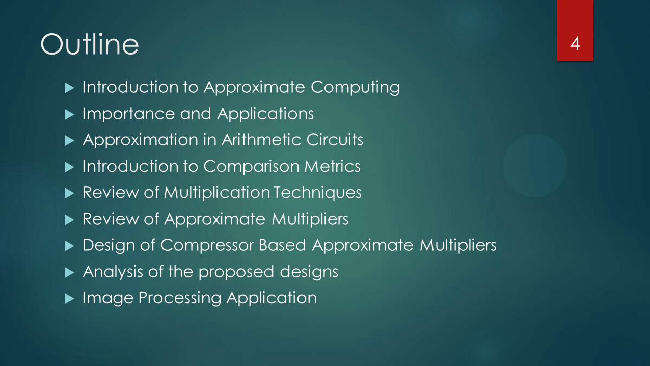
Introduction to Approximate Computing

Importance and Applications

Approximation in Arithmetic Circuits

Introduction to Comparison Metrics

Review of Multiplication Techniques

Review of Approximate Multipliers

Design of Compressor Based Approximate Multipliers

Analysis of the proposed designs

Image Processing Application

4

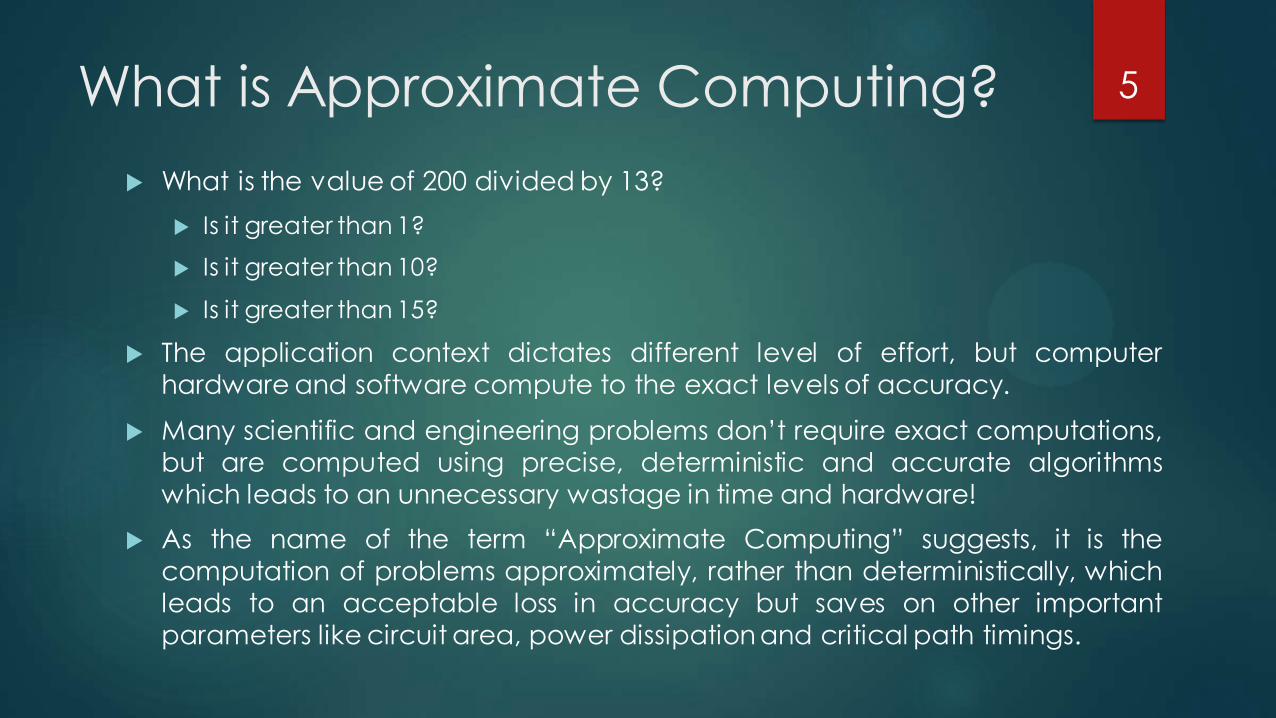
What is Approximate Computing?

What is the value of 200 divided by 13?

Is it greater than 1?

Is it greater than 10?

Is it greater than 15?

The application context dictates different level of effort, but computer

hardware and software compute to the exact levels of accuracy.

Many scientific and engineering problems don’t require exact computations,

but are computed using precise, deterministic and accurate algorithms

which leads to an unnecessary wastage in time and hardware!

As the name of the term “Approximate Computing” suggests, it is the

computation of problems approximately, rather than deterministically, which

leads to an acceptable loss in accuracy but saves on other important

parameters like circuit area, power dissipation and critical path timings.

5

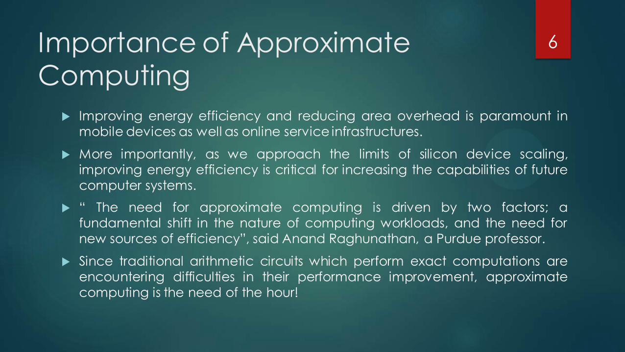
Importance of Approximate Computing

Improving energy efficiency and reducing area overhead is paramount in

mobile devices as well as online service infrastructures.

More importantly, as we approach the limits of silicon device scaling,

improving energy efficiency is critical for increasing the capabilities of future

computer systems.

“ The need for approximate computing is driven by two factors; a

fundamental shift in the nature of computing workloads, and the need for

new sources of efficiency”, said Anand Raghunathan, a Purdue professor.

Since traditional arithmetic circuits which perform exact computations are

encountering difficulties in their performance improvement, approximate

computing is the need of the hour!

6

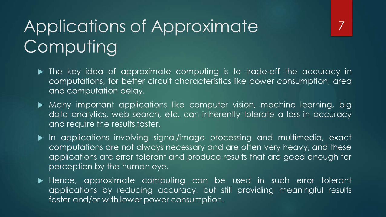
Applications of Approximate Computing

The key idea of approximate computing is to trade-off the accuracy in

computations, for better circuit characteristics like power consumption, area

and computation delay.

Many important applications like computer vision, machine learning, big

data analytics, web search, etc. can inherently tolerate a loss in accuracy

and require the results faster.

In applications involving signal/image processing and multimedia, exact

computations are not always necessary and are often very heavy, and these

applications are error tolerant and produce results that are good enough for

perception by the human eye.

Hence, approximate computing can be used in such error tolerant

applications by reducing accuracy, but still providing meaningful results

faster and/or with lower power consumption.

7

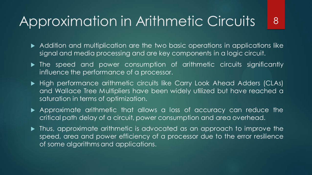
Approximation in Arithmetic Circuits

Addition and multiplication are the two basic operations in applications like

signal and media processing and are key components in a logic circuit.

The speed and power consumption of arithmetic circuits significantly

influence the performance of a processor.

High performance arithmetic circuits like Carry Look Ahead Adders (CLAs)

and Wallace Tree Multipliers have been widely utilized but have reached a

saturation in terms of optimization.

Approximate arithmetic that allows a loss of accuracy can reduce the

critical path delay of a circuit, power consumption and area overhead.

Thus, approximate arithmetic is advocated as an approach to improve the

speed, area and power efficiency of a processor due to the error resilience

of some algorithms and applications.

8

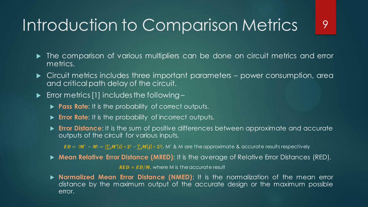
Introduction to Comparison Metrics

The comparison of various multipliers can be done on circuit metrics and error metrics.

Circuit metrics includes three important parameters – power consumption, area and critical path delay of the circuit.

Error metrics [1] includes the following –

Pass Rate: It is the probability of correct outputs.

Error Rate: It is the probability of incorrect outputs.

Error Distance: It is the sum of positive differences between approximate and accurate outputs of the circuit for various inputs.

𝑬𝑫 = ǀ𝑴′ − 𝑴ǀ = |∑𝒊𝑴′ 𝒊 ∗ 𝟐𝒊 −∑𝒋𝑴 𝒋 ∗ 𝟐

𝒋|, M’ & M are the approximate & accurate results respectively

Mean Relative Error Distance (MRED): It is the average of Relative Error Distances (RED).

𝑹𝑬𝑫 = 𝑬𝑫/𝑴, where M is the accurate result

Normalized Mean Error Distance (NMED): It is the normalization of the mean error distance by the maximum output of the accurate design or the maximum possible error.

9

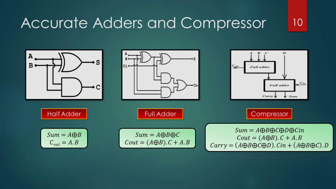
Accurate Adders and Compressor

Half Adder Full Adder Compressor

𝑆𝑢𝑚 = 𝐴⨁𝐵 𝐶𝑜𝑢𝑡 = 𝐴.𝐵

𝑆𝑢𝑚 = 𝐴⨁𝐵⨁𝐶 𝐶𝑜𝑢𝑡 = (𝐴⨁𝐵).𝐶 + 𝐴.𝐵

𝑆𝑢𝑚 = 𝐴⨁𝐵⨁𝐶⨁𝐷⨁𝐶𝑖𝑛 𝐶𝑜𝑢𝑡 = (𝐴⨁𝐵).𝐶 + 𝐴.𝐵

𝐶𝑎𝑟𝑟𝑦 = 𝐴⨁𝐵⨁𝐶⨁𝐷 .𝐶𝑖𝑛 + 𝐴⨁𝐵⨁𝐶 .𝐷

10

Review of Multipliers

A multiplier has a significant impact on the speed and power

dissipation of an arithmetic processor and hence, choosing the

appropriate multiplier design is very important.

Generally, a multiplier consists of stages of partial product generation,

accumulation and final addition.

There are three commonly used partial product accumulation

structures –

Wallace Tree

Dadda Tree

Carry-Save Adder Array

In the partial product accumulation stage, half adders, full adders or

compressors are used.

11

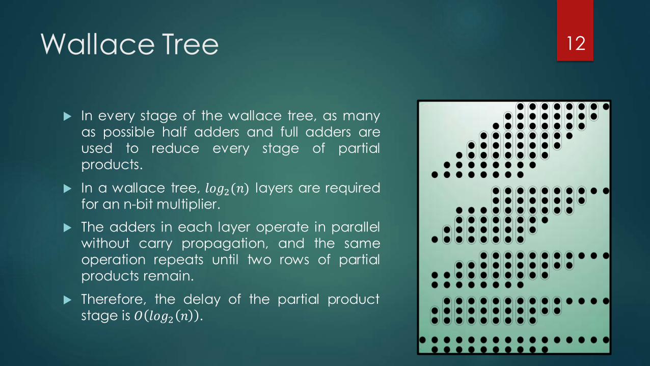
Wallace Tree

In every stage of the wallace tree, as many

as possible half adders and full adders are

used to reduce every stage of partial

products.

In a wallace tree, 𝑙𝑜𝑔2(𝑛) layers are required

for an n-bit multiplier.

The adders in each layer operate in parallel

without carry propagation, and the same

operation repeats until two rows of partial

products remain.

Therefore, the delay of the partial product

stage is 𝑂 𝑙𝑜𝑔2 𝑛 .

12

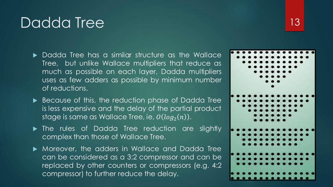
Dadda Tree

Dadda Tree has a similar structure as the Wallace

Tree, but unlike Wallace multipliers that reduce as

much as possible on each layer, Dadda multipliers

uses as few adders as possible by minimum number

of reductions.

Because of this, the reduction phase of Dadda Tree

is less expensive and the delay of the partial product

stage is same as Wallace Tree, ie, 𝑂 𝑙𝑜𝑔2 𝑛 .

The rules of Dadda Tree reduction are slightly

complex than those of Wallace Tree.

Moreover, the adders in Wallace and Dadda Tree

can be considered as a 3:2 compressor and can be

replaced by other counters or compressors (e.g. 4:2

compressor) to further reduce the delay.

13

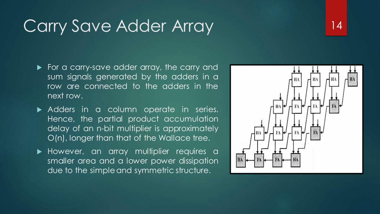
Carry Save Adder Array

For a carry-save adder array, the carry and

sum signals generated by the adders in a

row are connected to the adders in the

next row.

Adders in a column operate in series.

Hence, the partial product accumulation

delay of an n-bit multiplier is approximately

O(n), longer than that of the Wallace tree.

However, an array multiplier requires a

smaller area and a lower power dissipation

due to the simple and symmetric structure.

14

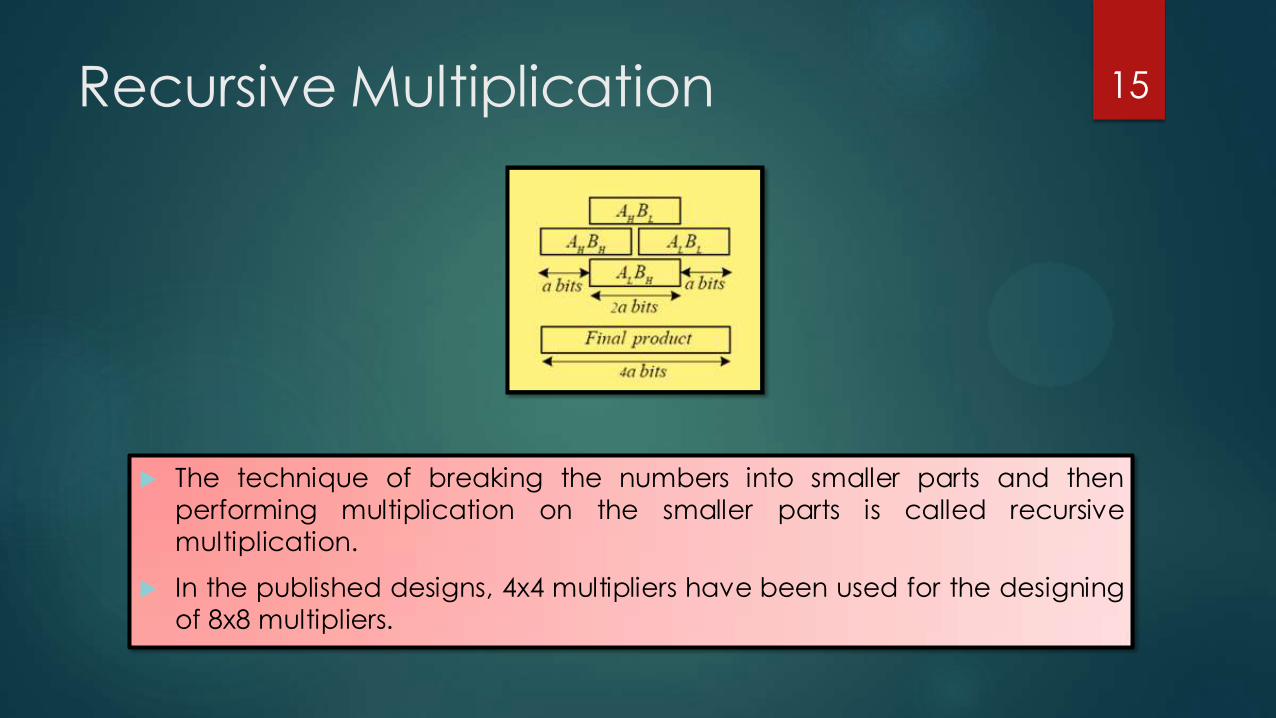
Recursive Multiplication

The technique of breaking the numbers into smaller parts and then

performing multiplication on the smaller parts is called recursive

multiplication.

In the published designs, 4x4 multipliers have been used for the designing

of 8x8 multipliers.

15

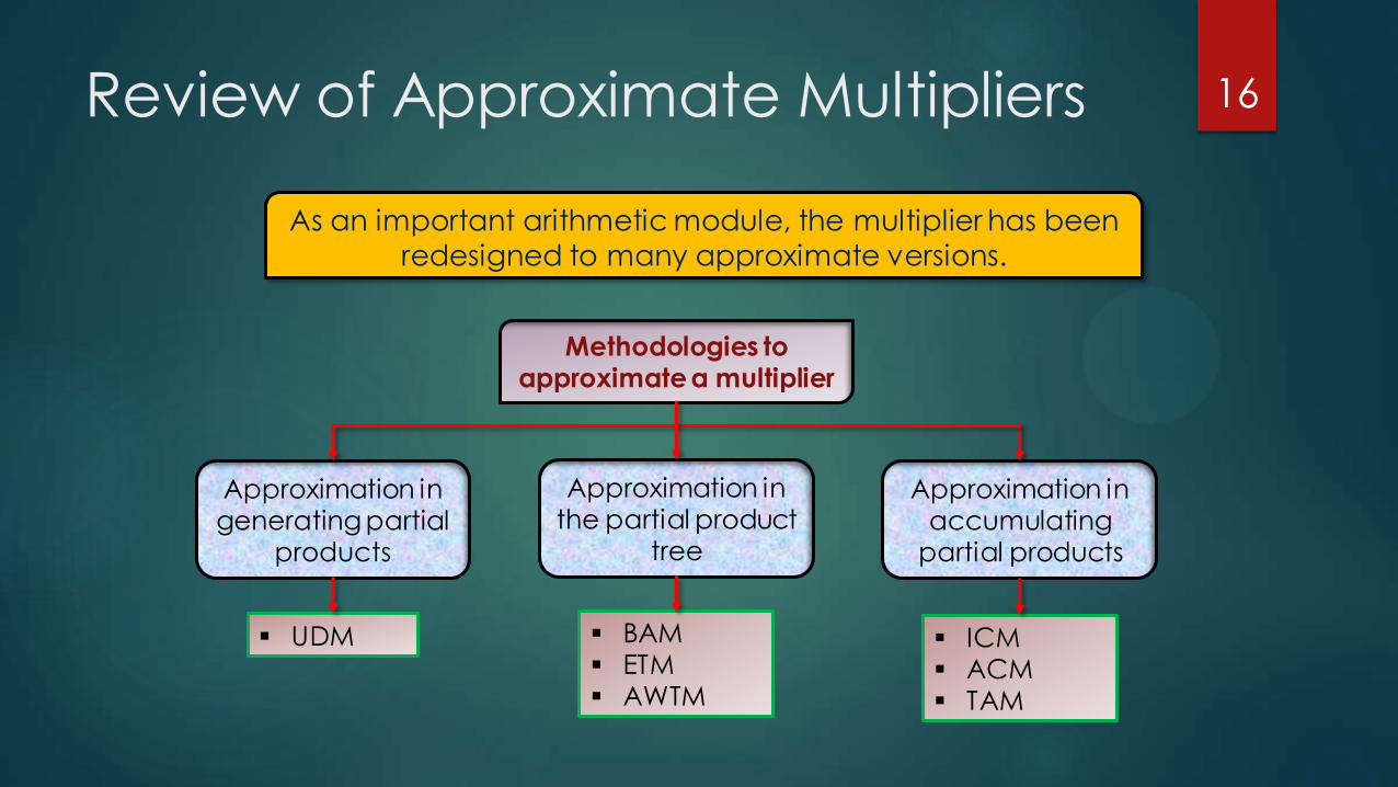
Review of Approximate Multipliers

As an important arithmetic module, the multiplier has been

redesigned to many approximate versions.

Methodologies to approximate a multiplier

Approximation in generating partial

products

Approximation in the partial product

tree

Approximation in accumulating

partial products

UDM ICM ACM TAM

BAM ETM AWTM

16

Under-Designed Multiplier (UDM) [2]

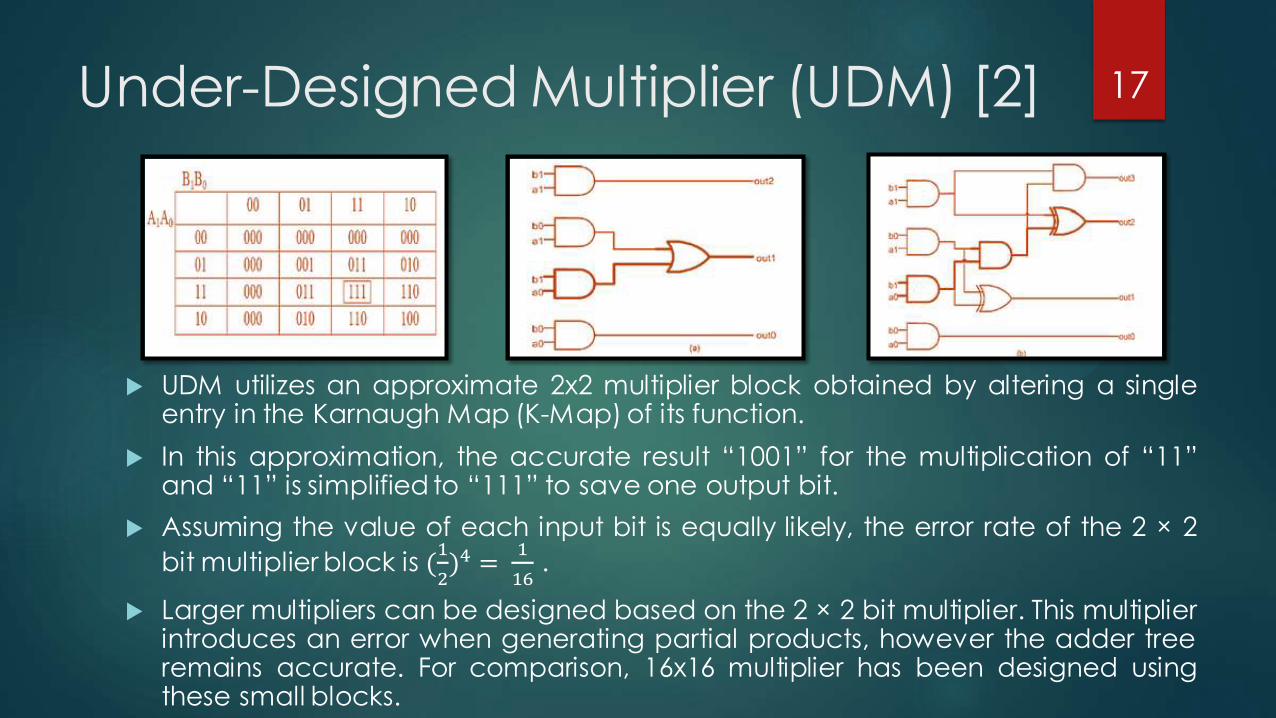
UDM utilizes an approximate 2x2 multiplier block obtained by altering a single entry in the Karnaugh Map (K-Map) of its function.

In this approximation, the accurate result “1001” for the multiplication of “11” and “11” is simplified to “111” to save one output bit.

Assuming the value of each input bit is equally likely, the error rate of the 2 × 2

bit multiplier block is (1

2)4 =

1

16 .

Larger multipliers can be designed based on the 2 × 2 bit multiplier. This multiplier introduces an error when generating partial products, however the adder tree remains accurate. For comparison, 16x16 multiplier has been designed using these small blocks.

17

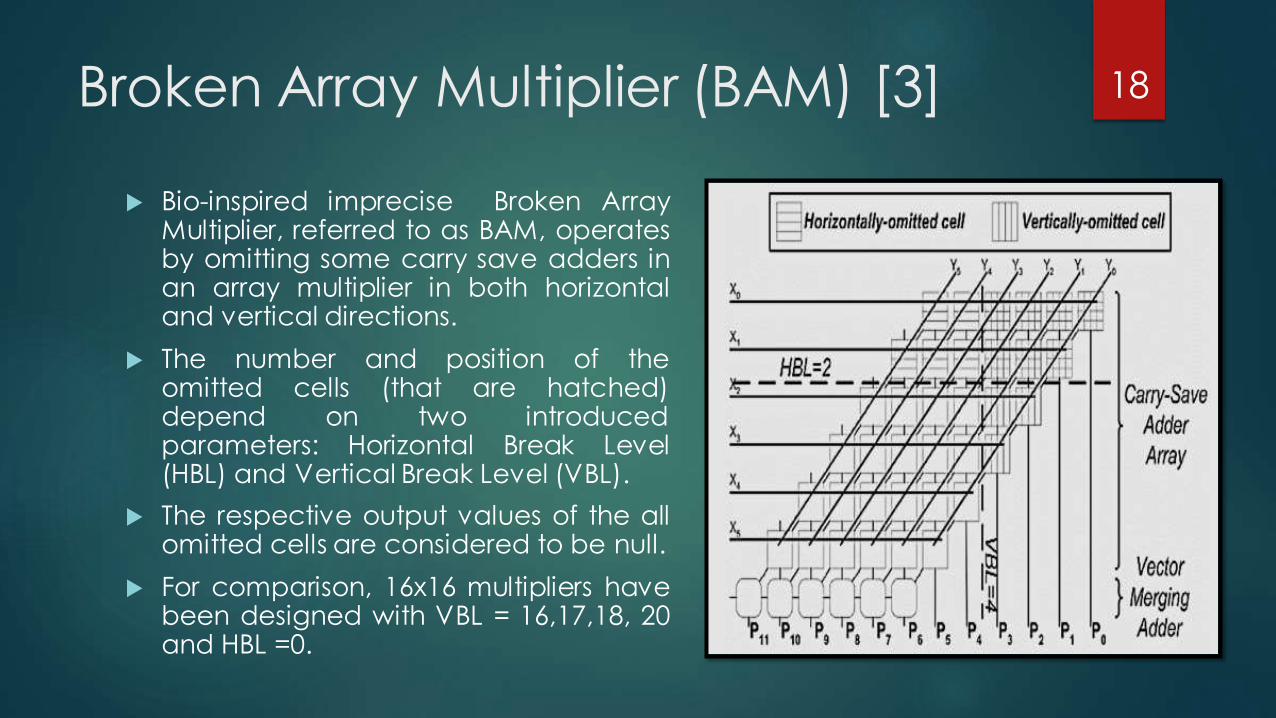
Broken Array Multiplier (BAM) [3]

Bio-inspired imprecise Broken Array Multiplier, referred to as BAM, operates by omitting some carry save adders in an array multiplier in both horizontal and vertical directions.

The number and position of the omitted cells (that are hatched) depend on two introduced parameters: Horizontal Break Level (HBL) and Vertical Break Level (VBL).

The respective output values of the all omitted cells are considered to be null.

For comparison, 16x16 multipliers have been designed with VBL = 16,17,18, 20 and HBL =0.

18

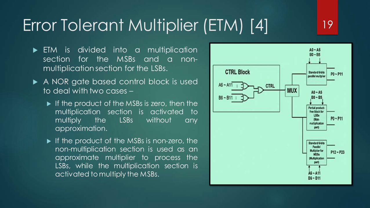
Error Tolerant Multiplier (ETM) [4]

ETM is divided into a multiplication

section for the MSBs and a non-

multiplication section for the LSBs.

A NOR gate based control block is used

to deal with two cases –

If the product of the MSBs is zero, then the multiplication section is activated to multiply the LSBs without any approximation.

If the product of the MSBs is non-zero, the non-multiplication section is used as an approximate multiplier to process the LSBs, while the multiplication section is activated to multiply the MSBs.

19

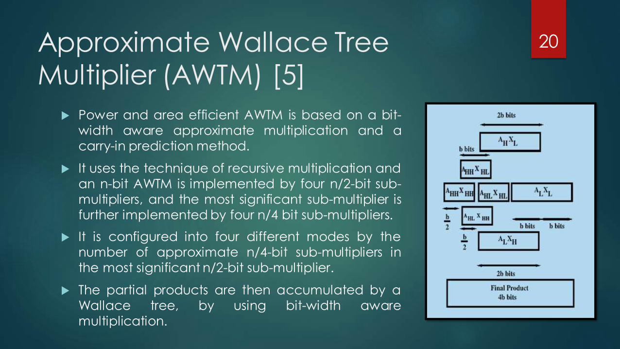
Approximate Wallace Tree Multiplier (AWTM) [5]

Power and area efficient AWTM is based on a bit-

width aware approximate multiplication and a

carry-in prediction method.

It uses the technique of recursive multiplication and

an n-bit AWTM is implemented by four n/2-bit sub-

multipliers, and the most significant sub-multiplier is

further implemented by four n/4 bit sub-multipliers.

It is configured into four different modes by the

number of approximate n/4-bit sub-multipliers in

the most significant n/2-bit sub-multiplier.

The partial products are then accumulated by a

Wallace tree, by using bit-width aware

multiplication.

20

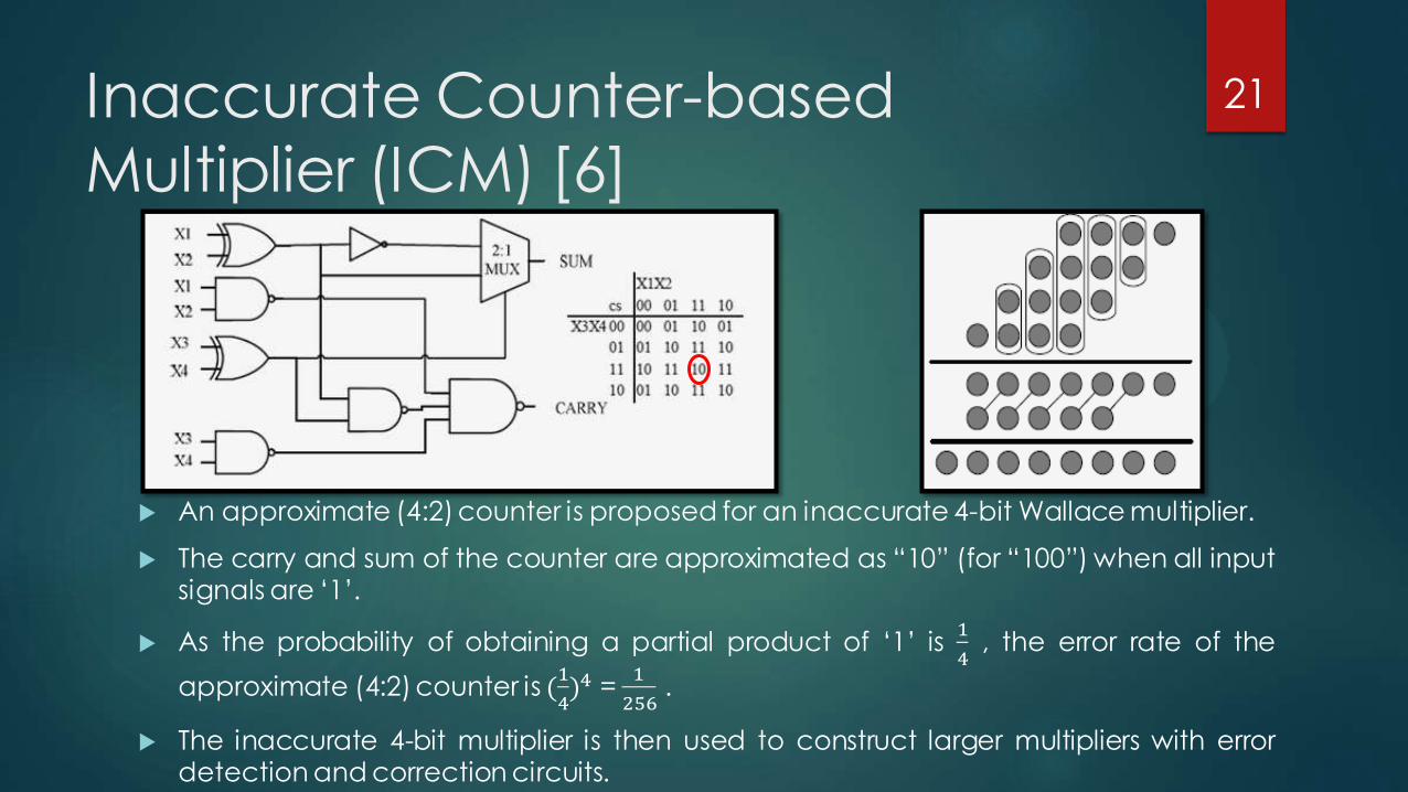
Inaccurate Counter-based Multiplier (ICM) [6]

An approximate (4:2) counter is proposed for an inaccurate 4-bit Wallace multiplier.

The carry and sum of the counter are approximated as “10” (for “100”) when all input signals are ‘1’.

As the probability of obtaining a partial product of ‘1’ is 1

4 , the error rate of the

approximate (4:2) counter is (1

4)4 =

1

256 .

The inaccurate 4-bit multiplier is then used to construct larger multipliers with error detection and correction circuits.

21

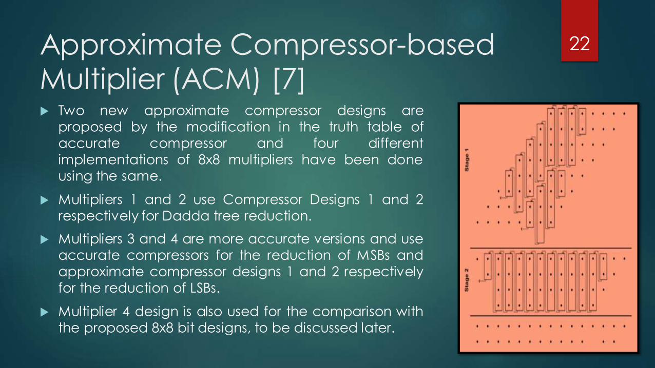
Approximate Compressor-based Multiplier (ACM) [7] Two new approximate compressor designs are

proposed by the modification in the truth table of

accurate compressor and four different

implementations of 8x8 multipliers have been done

using the same.

Multipliers 1 and 2 use Compressor Designs 1 and 2

respectively for Dadda tree reduction.

Multipliers 3 and 4 are more accurate versions and use

accurate compressors for the reduction of MSBs and

approximate compressor designs 1 and 2 respectively

for the reduction of LSBs.

Multiplier 4 design is also used for the comparison with

the proposed 8x8 bit designs, to be discussed later.

22

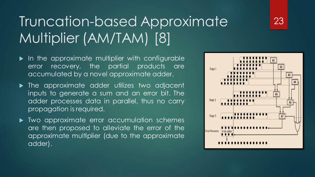
Truncation-based Approximate Multiplier (AM/TAM) [8]

In the approximate multiplier with configurable

error recovery, the partial products are

accumulated by a novel approximate adder.

The approximate adder utilizes two adjacent

inputs to generate a sum and an error bit. The

adder processes data in parallel, thus no carry

propagation is required.

Two approximate error accumulation schemes

are then proposed to alleviate the error of the

approximate multiplier (due to the approximate

adder).

23

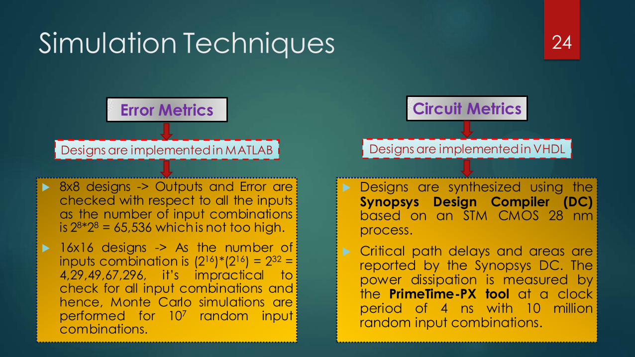
Simulation Techniques

8x8 designs -> Outputs and Error are checked with respect to all the inputs as the number of input combinations is 28*28 = 65,536 which is not too high.

16x16 designs -> As the number of inputs combination is (216)*(216) = 232 = 4,29,49,67,296, it’s impractical to check for all input combinations and hence, Monte Carlo simulations are performed for 107 random input combinations.

24

Error Metrics Circuit Metrics

Designs are implemented in MATLAB Designs are implemented in VHDL

Designs are synthesized using the Synopsys Design Compiler (DC) based on an STM CMOS 28 nm process.

Critical path delays and areas are reported by the Synopsys DC. The power dissipation is measured by the PrimeTime-PX tool at a clock period of 4 ns with 10 million random input combinations.

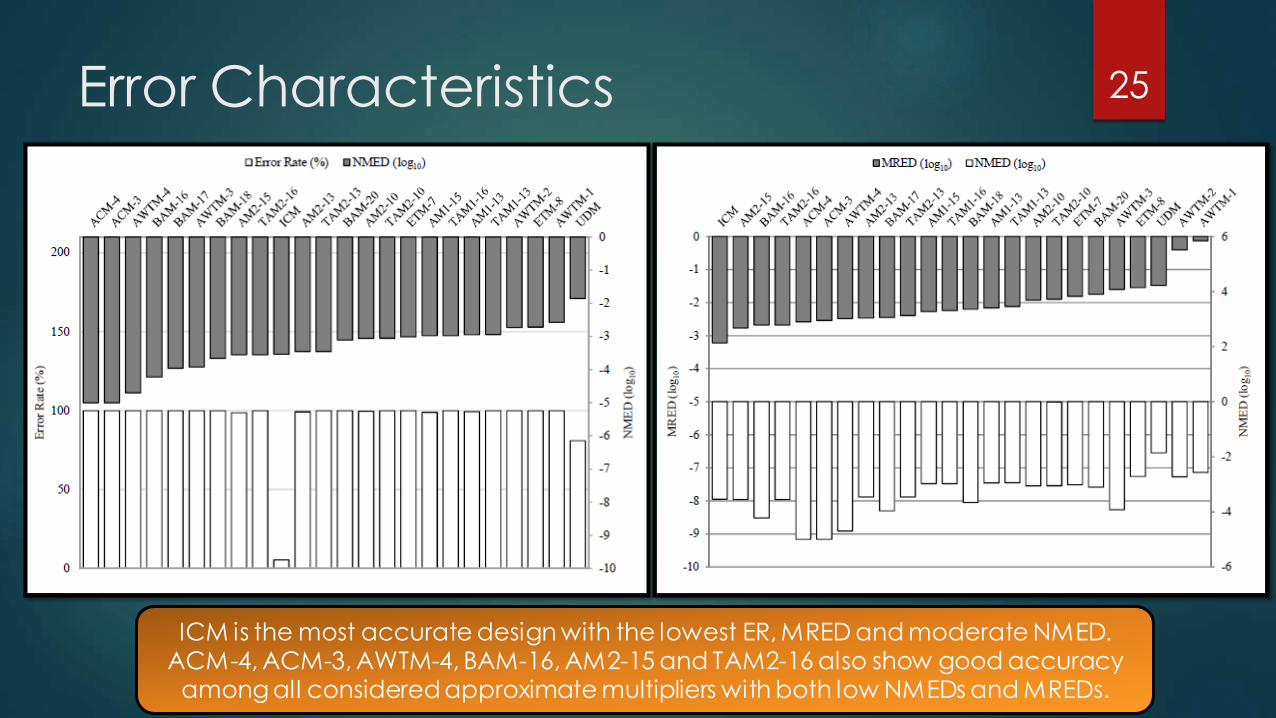
Error Characteristics 25

ICM is the most accurate design with the lowest ER, MRED and moderate NMED. ACM-4, ACM-3, AWTM-4, BAM-16, AM2-15 and TAM2-16 also show good accuracy

among all considered approximate multipliers with both low NMEDs and MREDs.

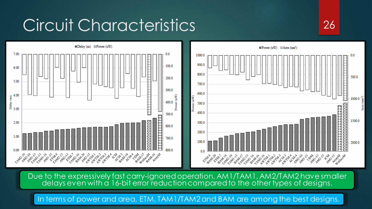
Circuit Characteristics

Due to the expressively fast carry-ignored operation, AM1/TAM1, AM2/TAM2 have smaller delays even with a 16-bit error reduction compared to the other types of designs.

26

In terms of power and area, ETM, TAM1/TAM2 and BAM are among the best designs.

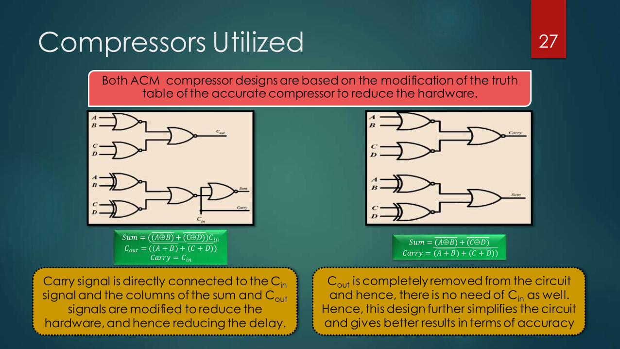
Compressors Utilized Both ACM compressor designs are based on the modification of the truth

table of the accurate compressor to reduce the hardware.

𝑆𝑢𝑚 = ((𝐴𝐵)+ (C𝐷))𝐶𝑖𝑛

𝐶𝑜𝑢𝑡 = ((𝐴 +𝐵)+ (𝐶 + 𝐷)) 𝐶𝑎𝑟𝑟𝑦 = 𝐶𝑖𝑛

𝑆𝑢𝑚 = (𝐴𝐵)+ (𝐶𝐷)

𝐶𝑎𝑟𝑟𝑦 = (𝐴 +𝐵)+ (𝐶 + 𝐷))

Carry signal is directly connected to the Cin signal and the columns of the sum and Cout

signals are modified to reduce the hardware, and hence reducing the delay.

Cout is completely removed from the circuit and hence, there is no need of Cin as well.

Hence, this design further simplifies the circuit and gives better results in terms of accuracy

27

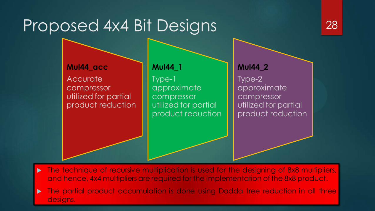
Proposed 4x4 Bit Designs

The technique of recursive multiplication is used for the designing of 8x8 multipliers, and hence, 4x4 multipliers are required for the implementation of the 8x8 product.

The partial product accumulation is done using Dadda tree reduction in all three designs.

Mul44_acc

Accurate compressor utilized for partial product reduction

Mul44_1

Type-1 approximate compressor utilized for partial product reduction

Mul44_2

Type-2 approximate compressor utilized for partial product reduction

28

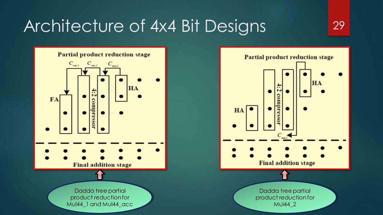
Architecture of 4x4 Bit Designs

Dadda tree partial product reduction for

Mul44_1 and Mul44_acc

Dadda tree partial product reduction for

Mul44_2

29

Proposed 8x8 Bit Designs

The partial product tree of the 8x8 multiplication is broken down to 4 products of 4x4 modules using the technique of recursive multiplication.

The advantage of breaking the products is to obtain smaller multiplication blocks that are performed in parallel and thus faster, and are merely required to be added.

30

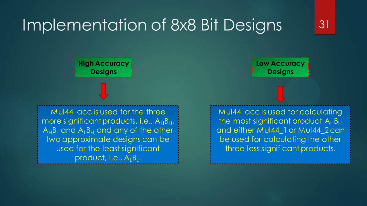
Implementation of 8x8 Bit Designs

Mul44_acc is used for the three

more significant products, i.e., AHBH,

AHBL and ALBH, and any of the other

two approximate designs can be

used for the least significant

product, i.e., ALBL.

31

High Accuracy Designs

Low Accuracy Designs

Mul44_acc is used for calculating

the most significant product AHBH

and either Mul44_1 or Mul44_2 can

be used for calculating the other

three less significant products.

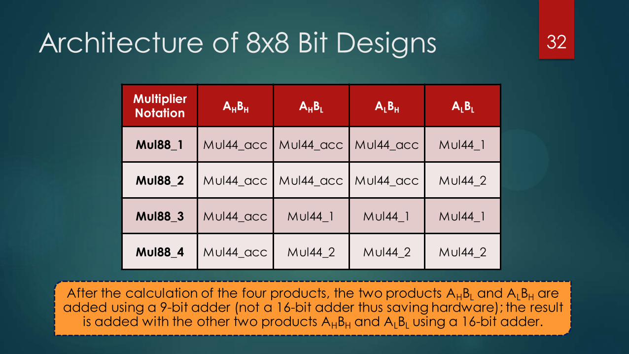
Architecture of 8x8 Bit Designs 32

After the calculation of the four products, the two products AHBL and ALBH are added using a 9-bit adder (not a 16-bit adder thus saving hardware); the result

is added with the other two products AHBH and ALBL using a 16-bit adder.

Multiplier Notation

AHBH AHBL ALBH ALBL

Mul88_1 Mul44_acc Mul44_acc Mul44_acc Mul44_1

Mul88_2 Mul44_acc Mul44_acc Mul44_acc Mul44_2

Mul88_3 Mul44_acc Mul44_1 Mul44_1 Mul44_1

Mul88_4 Mul44_acc Mul44_2 Mul44_2 Mul44_2

Metrics for 4x4 Bit Designs

Mul44_2 is better than Mul44_1 in terms of accuracy, giving an indication of design 2 compressor being better than design 1.

33

Design Power (W)

Delay (ns)

Area (m2)

Mul44_1 18.746 1.49 138.32

Mul44_2 20.8905 1.43 139.36

Mul44_acc 29.8582 1.66 166.39

Design Average

NED

Pass Rate (%)

Error Rate (%)

Mul44_1 0.0503 32.42 67.58

Mul44_2 0.0139 60.93 39.07

Mul44_acc 0 100 0

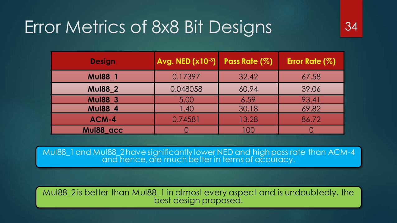
Error Metrics of 8x8 Bit Designs

Mul88_1 and Mul88_2 have significantly lower NED and high pass rate than ACM-4 and hence, are much better in terms of accuracy.

34

Design Avg. NED (x10-3) Pass Rate (%) Error Rate (%)

Mul88_1 0.17397 32.42 67.58

Mul88_2 0.048058 60.94 39.06

Mul88_3 5.00 6.59 93.41

Mul88_4 1.40 30.18 69.82

ACM-4 0.74581 13.28 86.72

Mul88_acc 0 100 0

Mul88_2 is better than Mul88_1 in almost every aspect and is undoubtedly, the best design proposed.

Circuit Metrics of 8x8 Bit Designs

Proposed designs have significantly better area, power and delay than reference accurate design and also, less power and delay than ACM-4 design discussed before.

35

Design Power (W) Delay (ns) Area (m2)

Mul88_1 168.7982 2.97 808.5999

Mul88_2 170.8133 2.91 809.6399

Mul88_3 140.7181 2.97 752.4399

Mul88_4 151.3424 2.91 755.5599

ACM-4 176.4869 3.13 727.999

Mul88_acc 179.7635 3.14 836.6799

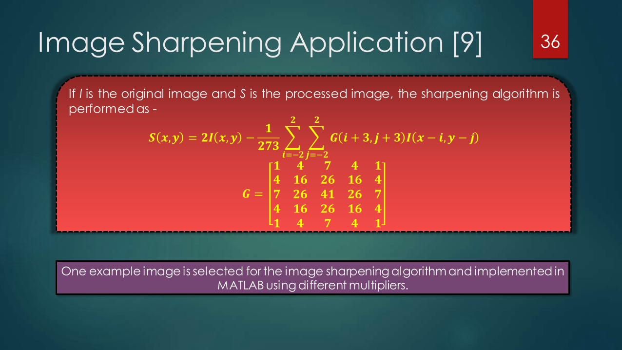
Image Sharpening Application [9]

If I is the original image and S is the processed image, the sharpening algorithm is

performed as -

𝑺 𝒙,𝒚 = 𝟐𝑰 𝒙,𝒚 −𝟏

𝟐𝟕𝟑 𝑮 𝒊 + 𝟑, 𝒋 + 𝟑 𝑰 𝒙 − 𝒊,𝒚 − 𝒋

𝟐

𝒋=−𝟐

𝟐

𝒊=−𝟐

𝑮 =

𝟏 𝟒 𝟕 𝟒 𝟏𝟒 𝟏𝟔 𝟐𝟔 𝟏𝟔 𝟒𝟕 𝟐𝟔 𝟒𝟏 𝟐𝟔 𝟕𝟒 𝟏𝟔 𝟐𝟔 𝟏𝟔 𝟒𝟏 𝟒 𝟕 𝟒 𝟏

36

One example image is selected for the image sharpening algorithm and implemented in MATLAB using different multipliers.

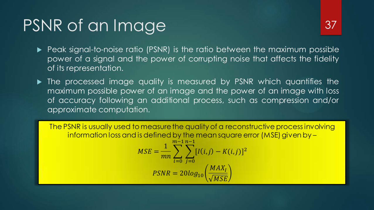
PSNR of an Image

Peak signal-to-noise ratio (PSNR) is the ratio between the maximum possible

power of a signal and the power of corrupting noise that affects the fidelity

of its representation.

The processed image quality is measured by PSNR which quantifies the

maximum possible power of an image and the power of an image with loss

of accuracy following an additional process, such as compression and/or

approximate computation.

37

The PSNR is usually used to measure the quality of a reconstructive process involving information loss and is defined by the mean square error (MSE) given by –

𝑀𝑆𝐸 =1

𝑚𝑛 [𝐼 𝑖, 𝑗 − 𝐾(𝑖, 𝑗)]2𝑛−1

𝑗=0

𝑚−1

𝑖=0

𝑃𝑆𝑁𝑅 = 20𝑙𝑜𝑔10𝑀𝐴𝑋𝐼

𝑀𝑆𝐸

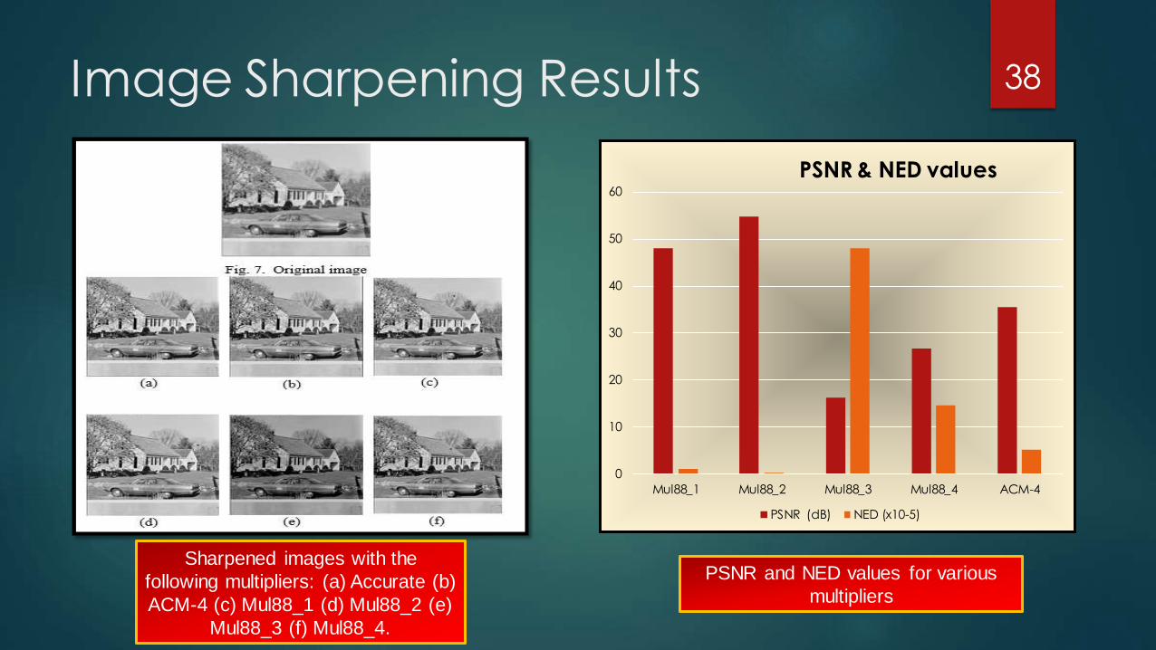
Image Sharpening Results

PSNR and NED values for various

multipliers

38

Sharpened images with the

following multipliers: (a) Accurate (b)

ACM-4 (c) Mul88_1 (d) Mul88_2 (e)

Mul88_3 (f) Mul88_4.

0

10

20

30

40

50

60

Mul88_1 Mul88_2 Mul88_3 Mul88_4 ACM-4

PSNR & NED values

PSNR (dB) NED (x10-5)

Conclusion

Approximate computing is a new and interesting paradigm that is well suited

for arithmetic circuits to reduce power, area and delay, while keeping the

accuracy at an acceptable level.

For an error resilient systems and applications like signal and media

processing, approximate arithmetic circuits offer several advantages such as

lower power consumption and faster processing.

Review of the existing multiplier designs is a must and can be used to

determine the suitable design according to the application requirements.

The proposed Mul88_1 and Mul88_2 achieve improvements of 76.67% &

93.55% for accuracy, and 4.36% & 3.21% for power over ACM-4 design.

39

In summary, the first two proposed designs, Mul88_1 and Mul88_2, are suitable for error tolerant applications that require a high accuracy; Mul88_2 achieves the most

accurate result. The other two designs, Mul88_3 and Mul88_4, are suited for low power applications in which a larger degradation in accuracy can be tolerated.

40

E-Mail: naman.mah1993@gmail.com

References [1] J. Liang, J. Han, F. Lombardi, “New metrics for the reliability of approximate and probabilistic adders,” IEEE Trans. on Computers, vol. 63, no. 9, pp. 1760 - 1771, 2013.

[2] P. Kulkarni, P. Gupta, M. Ercegovac, "Trading accuracy for power with an Underdesigned Multiplier architecture," 24th International Conference on VLSI Design, 2011.

[3] H.R. Mahdiani, A. Ahmadi, S.M. Fakhraie, C. Lucas, "Bio-Inspired imprecise computational blocks for efficient VLSI implementation of soft-computing applications," IEEE Transactions on Circuits and Systems, vol. 57 no. 4, 2010.

[4] K.Y. Kyaw, W.L. Goh, K.S. Yeo, "Low-power high-speed multiplier for error-tolerant application," IEEE International Conference of Electron Devices and Solid-State Circuits (EDSSC), 2010.

[5] K. Bhardwaj, P.S. Mane, J. Henkel, "Power- and area-efficient Approximate Wallace Tree Multiplier for error-resilient systems," 15th International Symposium on Quality Electronic Design (ISQED), 2014.

[6] C.-H. Lin, I.-C. Lin, "High accuracy approximate multiplier with error correction," IEEE 31st International Conference on Computer Design (ICCD), 2013.

[7] A. Momeni, J. Han, P. Montuschi, F. Lombardi, "Design and analysis of approximate compressors for multiplication," IEEE Transactions on Computers, in press, 2014.

[8] C. Liu, J. Han and F. Lombardi, “A Low-Power, High-Performance Approximate Multiplier with Configurable Partial Error Recovery,” DATE 2014, Dresten, Germany, 2014.

[9] M.S.K Lau, K.V. Ling, Y.C. Chu. "Energy-aware probabilistic multiplier: design and analysis." In Proceedings of the 2009 international conference on Compilers, architecture, and synthesis for embedded systems, Grenoble, France, pp. 281-290, 2009.

41