Cankaya University Journal of Science and Engineering

Volume 9 (2012), No. 2, 139–147

Approximate Analytical Solutions of theFractional Sharma-Tasso-Olver Equation UsingHomotopy Analysis Method and a Comparison

with Other Methods

Alaattin Esen1,∗, Orkun Tasbozan1 and N. Murat Yagmurlu1

1Inonu University, Faculty of Art and Sciences, Department of Mathematics, 44280 Malatya, Turkey∗Corresponding author: aesen@inonu.edu.tr

Ozet. Bu calısmada, kesirli mertebeden Sharma-Tasso-Olver (STO) denkleminin yaklasıkanalitik cozumlerini elde etmek icin homotopi analiz metodu (HAM) basarılı bir sekildeuygulandı. Elde edilen sonuclarla varyasyonel iterasyon metodu (VIM), Adomian ayrıstır-ma metodu (ADM) ve homotopi perturbasyon metodu (HPM) ile elde edilen sonuclarınkarsılastırılması; onemli olcude anlamlı sonuclar elde ettigimiz sonucuna varmamıza sebepoldu. HAM cozumu, cozum serilerinin yakınsaklık bolgesini kontrol etmek ve ayarlamakicin uygun bir yol saglayan bir ~ yardımcı parametresini icerir.

Anahtar Kelimeler. Homotopi analiz metodu, yaklasık analitik cozum, kesirli mertebe-den Sharma-Tasso-Olver denklemi, kesirli kalkulus.

Abstract. In this paper, the homotopy analysis method (HAM) is successfully applied tothe fractional Sharma-Tasso-Olver equation to obtain its approximate analytical solutions.Comparison of the obtained results with those of variational iteration method (VIM),Adomian’s decomposition method (ADM) and homotopy perturbation method (HPM) hasled us to conclude that the method gives significantly important consequences. The HAMsolution includes an auxiliary parameter ~ which provides a convenient way of adjustingand controlling the convergence region of solution series.

Keywords. Homotopy analysis method, approximate analytical solution, fractionalSharma-Tasso-Olver equation, fractional calculus.

1. Introduction

Since many important phenomena in physics and engineering can only be well de-

scribed by fractional differential equations, a considerable interest in them has been

aroused recently due to their widespread applications in physics and engineering.

However, in general, there exists no method that gives an exact solution for a frac-

tional differential equation. Thus, their approximate analytical solutions have been

Received March 20, 2012; accepted February 6, 2013.

ISSN 1309 - 6788 © 2013 Cankaya University

140 Esen et al.

sought and found by various methods such as VIM [1, 2], ADM [3, 4], HPM [5, 6]

and HAM [7, 8, 9]. The HAM which was first proposed by Liao [10, 11] is a pow-

erful tool for searching the approximate solutions of nonlinear evolution equations

(NLEEs). Unlike perturbation techniques, the HAM is not limited to any small

physical parameters in the considered equation. Therefore, the HAM can overcome

the foregoing restrictions and limitations of perturbation techniques so that it pro-

vides us with a powerful tool to analyze strongly nonlinear problems [12, 13]. In this

paper, we will apply the HAM to the fractional Sharma-Tasso-Olver equation. One

of the fractional differential equations arising in science and engineering is Sharma-

Tasso-Olver equation with time-fractional derivative of the form

Dαt u+ 3au2x + 3au2ux + 3auuxx + auxxx = 0, t > 0, 0 < α ≤ 1 (1)

where a is an arbitary constant, α is a parameter describing the order of the frac-

tional time-derivative.

Several definitions of fractional integration and derivation such as Riemann-

Liouville’s and Casputo’s have been proposed. The Riemann-Liouville integral op-

erator [14] having order α > 0 is defined as

Jαf(x) =1

Γ(α)

xˆ

0

(x− t)α−1f(t)dt (x > 0)

and as

J0f(x) = f(x)

for α = 0. Its fractional derivative of order α > 0 is generally used

Dαf(x) =dn

dxnJn−αf(x) (n− 1 < α < n)

where n is an arbitrary integer. The Riemann-Liouville integral operator has an

important role for the development of the theory of both fractional derivatives and

integrals. In spite of this fact, it has certain disadvantages when it comes to mod-

elling real-world phenomena with fractional differential equations. This problem has

been solved by M. Caputo first in his article [15] and then in his book [16]. Caputo

definition, which is a modification of Riemann-Liouville definition, can be given as

Dαf(x) = Jn−αDnf(x) =1

Γ(n− α)

xˆ

0

(x−t)n−α−1f (n)(t)dt, α > 0, (n−1 < α < n).

CUJSE 9 (2012), No. 2 141

Note that Caputo derivative has the following two important properties

DαJαf (x) = f (x)

and

JαDαf(x) = f(x)−n−1∑k=0

f (k)(0+)xk

k!(n− 1 < α < n).

2. HAM Solutions of Fractional Sharma-Tasso-Olver

Equation

The Eq. (1) is considered with the initial condition

u(x, 0) =2k(w + tanh(kx))

1 + w tanh(kx)(2)

where k, w ∈ C. To investigate the series solution of Eq. (1) with initial condition

(2) and to make a comparison with VIM, ADM and HPM solutions in Ref. [17], we

choose the linear operator

L [φ(x, t; q)] = Dαt [φ(x, t; q)]

with the property

L [c] = 0

where c is constant. From Eq. (1), we can now define a nonlinear operator as

N [φ(x, t; q)] =∂αφ(x, t; q)

∂tα+ 3a

(∂φ(x, t; q)

∂x

)2

+ 3a (φ(x, t; q))2∂φ(x, t; q)

∂x+ 3aφ(x, t; q)

∂2φ(x, t; q)

∂x2+ a

∂3φ(x, t; q)

∂x3.

Therefore, we construct the zero-order deformation equation as follows

(1− q)L[φ(x, t; q)− u0(x, t)] = q}N [φ(x, t; q)]. (3)

Obviously, if we choose q = 0 and q = 1, then we obtain

φ(x, t; 0) = u0(x, t) = u(x, 0),

φ(x, t; 1) = u(x, t)

respectively. Thus, as the embedding parameter q increases from 0 to 1, the solution

142 Esen et al.

φ(x, t; q) varies from the initial value u0(x, t) to the solution u(x, t). By expanding

φ(x, t; q) in Taylor series with respect to the embedding parameter q, we obtain

φ(x, t; q) = u0(x, t) +∞∑m=1

um(x, t)qm

where

um(x, t) =1

m!

∂mφ(x, t; q)

∂qm

∣∣∣∣q=0

.

If the auxiliary linear operator, the initial guess and the auxiliary parameter ~ are

properly chosen, the above series converges at q = 1, and one can have

u(x, t) = u0(x, t) +∞∑m=1

um(x, t)

which must be one of the solutions of the original nonlinear equation, as proved by

Liao [11, 18]. By differentiating Eq. (3) m times with respect to the embedding

parameter q, we obtain the mth-order deformation equation

L [um(x, t)− χmum−1(x, t)] = ~Rm (~um−1) (4)

where

Rm(~um−1) =∂αum−1(x, t)

∂tα+ 3a

m−1∑n=0

∂un(x, t)

∂x

∂um−1−n(x, t)

∂x

+ 3am−1∑n=0

(n∑k=0

uk(x, t)un−k(x, t)

)∂um−1−n(x, t)

∂x

+ 3am−1∑n=0

un(x, t)∂2um−1−n(x, t)

∂x2+ a

∂3um−1(x, t)

∂x3

and

χm =

{0, m ≤ 1,

1, m > 1.

The solution of the mth-order deformation Eq. (4) for m ≥ 1 leads to

um(x, t) = χmum−1(x, t) + ~Jαt [Rm (~um−1)] . (5)

By using Eq. (5) with the initial condition given by (2), we successively obtain

u0(x, t) = u(x, 0) =2k(w + tanh(kx))

1 + w tanh(kx),

CUJSE 9 (2012), No. 2 143

u1(x, t) =16ak4(w2 − 1)2~tα

Γ(α + 1)(cosh(kx) + w sinh(kx))4+

8ak4(w4 − 1)~tα cosh(2kx)

Γ(α + 1)(cosh(kx) + w sinh(kx))4

+16ak4w(w2 − 1)~tα sinh(2kx)

Γ(α + 1)(cosh(kx) + w sinh(kx))4,

...

etc. Therefore, the series solution expressed by the HAM can be written in the form

u(x, t) = u0(x, t) + u1(x, t) + u2(x, t) + u3(x, t) + . . . . (6)

To demonstrate the efficiency of the method, we compare the HAM solutions of

fractional Sharma-Tasso-Olver equation given by Eq. (6) for α = 1 with exact

solutions [17]

u(x, t) =2k(w + tanh(k(x− 4ak2t)))

1 + w tanh(k(x− 4ak2t)). (7)

Note that our HAM solution series contains the auxiliary parameter ~ which pro-

vides us with a simply way to adjust and control the convergence of the solution

series. To obtain an appropriate range for ~, we consider the so-called ~-curve to

choose a proper value of ~ which ensures that the solution series is convergent, as

pointed by Liao [11], by discovering the valid region of ~ which corresponds to the

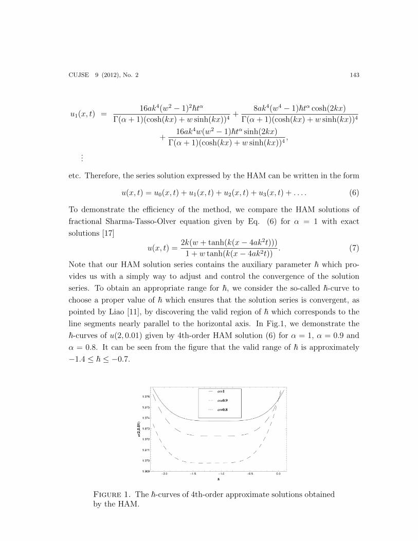
line segments nearly parallel to the horizontal axis. In Fig.1, we demonstrate the

~-curves of u(2, 0.01) given by 4th-order HAM solution (6) for α = 1, α = 0.9 and

α = 0.8. It can be seen from the figure that the valid range of ~ is approximately

−1.4 ≤ ~ ≤ −0.7.

Figure 1. The ~-curves of 4th-order approximate solutions obtainedby the HAM.

144 Esen et al.

The comparison of the results of the HAM, VIM [17], ADM [17], HPM [17] and

exact solution for α = 1 is given in Table 1. It shows that 4th-order approximate

solution obtained by the HAM for ~ = −1 is in good agrement at almost all points

(x, t).

Table 1. The results obtained by the HAM for ~ = −1 by 4th-orderapproximate solution in comparison with the VIM, ADM, HPM inRef. [17] and exact solution at t = 0.01 for α = k = a = 1, and w = 1

2.

x uVIM [17] uADM [17] uHPM [17] uHAM(x, t) Exact Solution0 0.938798380 0.938800000 0.938800000 0.938808800 0.9388088081 1.813642383 1.813642415 1.813642415 1.813631681 1.8136316812 1.973721044 1.973721044 1.973721044 1.973719022 1.9737190223 1.996423221 1.996423221 1.996423221 1.996422935 1.9964229354 1.999515561 1.999515561 1.999515561 1.999515522 1.9995155225 1.999934431 1.999934431 1.999934431 1.999934426 1.9999344266 1.999991127 1.999991127 1.999991127 1.999991125 1.9999911257 1.999998799 1.999998799 1.999998799 1.999998799 1.9999987998 1.999999839 1.999999839 1.999999839 1.999999837 1.9999998379 1.999999978 1.999999978 1.999999978 1.999999978 1.999999978

10 1.999999997 1.999999997 1.999999997 1.999999997 1.999999997

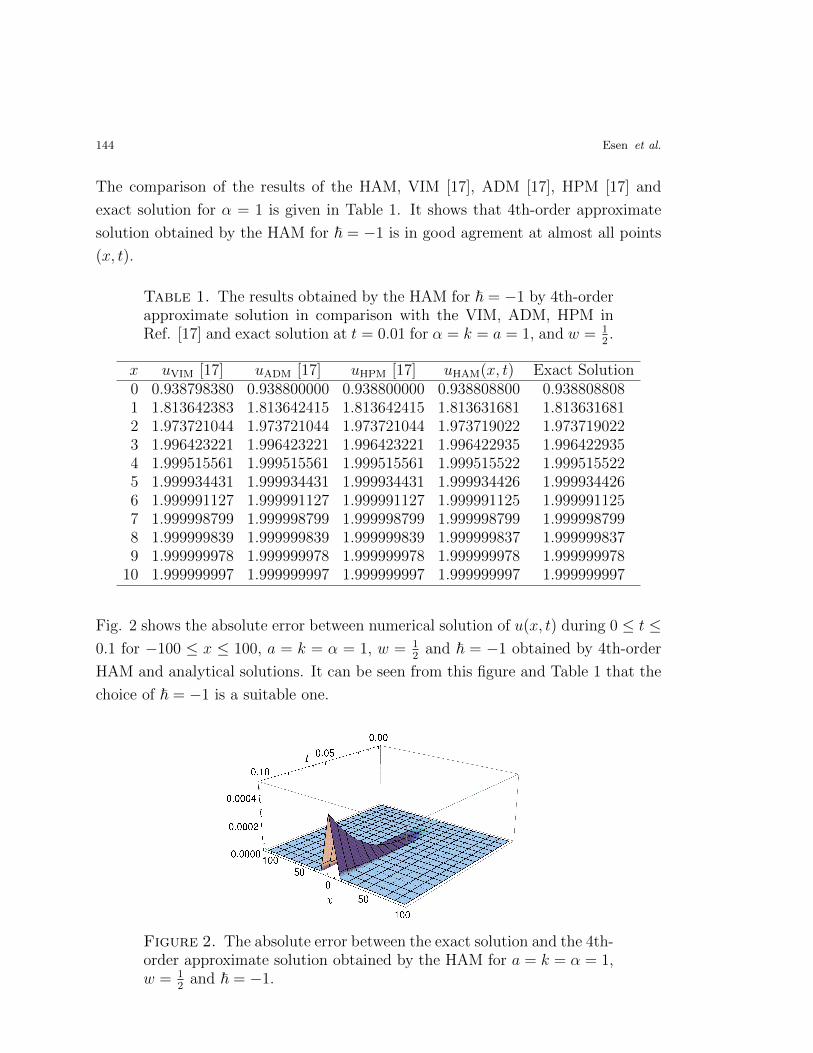
Fig. 2 shows the absolute error between numerical solution of u(x, t) during 0 ≤ t ≤0.1 for −100 ≤ x ≤ 100, a = k = α = 1, w = 1

2and ~ = −1 obtained by 4th-order

HAM and analytical solutions. It can be seen from this figure and Table 1 that the

choice of ~ = −1 is a suitable one.

Figure 2. The absolute error between the exact solution and the 4th-order approximate solution obtained by the HAM for a = k = α = 1,w = 1

2and ~ = −1.

CUJSE 9 (2012), No. 2 145

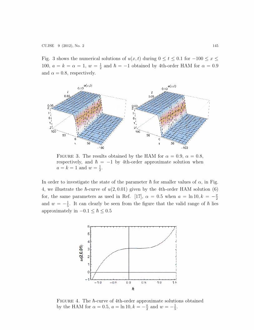
Fig. 3 shows the numerical solutions of u(x, t) during 0 ≤ t ≤ 0.1 for −100 ≤ x ≤100, a = k = α = 1, w = 1

2and ~ = −1 obtained by 4th-order HAM for α = 0.9

and α = 0.8, respectively.

Figure 3. The results obtained by the HAM for α = 0.9, α = 0.8,respectively, and ~ = −1 by 4th-order approximate solution whena = k = 1 and w = 1

2.

In order to investigate the state of the parameter ~ for smaller values of α, in Fig.

4, we illustrate the ~-curve of u(2, 0.01) given by the 4th-order HAM solution (6)

for, the same parameters as used in Ref. [17], α = 0.5 when a = ln 10, k = −π2

and w = −15. It can clearly be seen from the figure that the valid range of ~ lies

approximately in −0.1 ≤ ~ ≤ 0.5

Figure 4. The ~-curve of 4th-order approximate solutions obtainedby the HAM for α = 0.5, a = ln 10, k = −π

2and w = −1

5.

146 Esen et al.

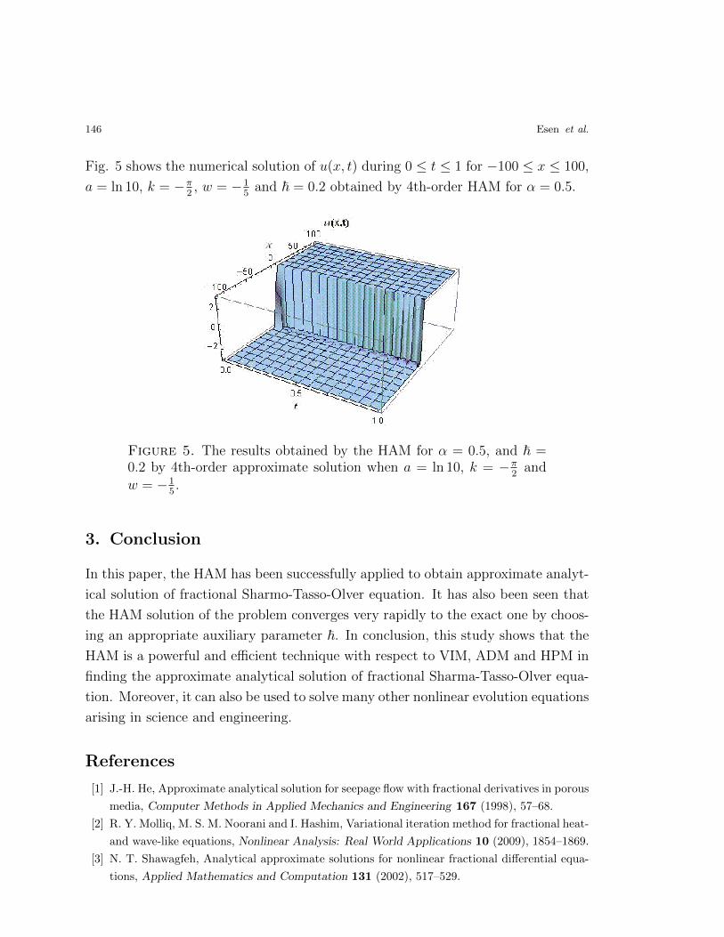
Fig. 5 shows the numerical solution of u(x, t) during 0 ≤ t ≤ 1 for −100 ≤ x ≤ 100,

a = ln 10, k = −π2, w = −1

5and ~ = 0.2 obtained by 4th-order HAM for α = 0.5.

Figure 5. The results obtained by the HAM for α = 0.5, and ~ =0.2 by 4th-order approximate solution when a = ln 10, k = −π

2and

w = −15.

3. Conclusion

In this paper, the HAM has been successfully applied to obtain approximate analyt-

ical solution of fractional Sharmo-Tasso-Olver equation. It has also been seen that

the HAM solution of the problem converges very rapidly to the exact one by choos-

ing an appropriate auxiliary parameter ~. In conclusion, this study shows that the

HAM is a powerful and efficient technique with respect to VIM, ADM and HPM in

finding the approximate analytical solution of fractional Sharma-Tasso-Olver equa-

tion. Moreover, it can also be used to solve many other nonlinear evolution equations

arising in science and engineering.

References

[1] J.-H. He, Approximate analytical solution for seepage flow with fractional derivatives in porous

media, Computer Methods in Applied Mechanics and Engineering 167 (1998), 57–68.

[2] R. Y. Molliq, M. S. M. Noorani and I. Hashim, Variational iteration method for fractional heat-

and wave-like equations, Nonlinear Analysis: Real World Applications 10 (2009), 1854–1869.

[3] N. T. Shawagfeh, Analytical approximate solutions for nonlinear fractional differential equa-

tions, Applied Mathematics and Computation 131 (2002), 517–529.

CUJSE 9 (2012), No. 2 147

[4] S. Momani and Z. Obibat, Numerical approach to differential equations of fractional order,

Journal of Computational and Applied Mathematics 207 (2007), 96–110.

[5] S. Momani and Z. Odibat, Homotopy perturbation method for nonlinear partial differential

equations of fractional order, Physics Letters A 365 (2007), 345–350.

[6] Z. Odibat, Exact solitary solutions for variants of the KdV equations with fractional time

derivatives, Chaos, Solitons & Fractals 40 (2009), 1264–1270.

[7] H. Xu and J. Cang, Analysis of a time fractional wave-like equation with the homotopy analysis

method, Physics Letters A 372 (2008), 1250–1255.

[8] L. Song and H. Q. Zhang, Application of homotopy analysis method to fractional KdV-

Burgers-Kuramoto equation, Physics Letters A 367 (2007), 88–94.

[9] H. Jafari and S. Seifi, Homotopy analysis method for solving linear and nonlinear fractional

diffusion-wave equation, Communications in Nonlinear Science and Numerical Simulation 14

(2009), 2006–2012.

[10] S. J. Liao, The Proposed Homotopy Analysis Tecnique for the Solution of Nonlinear Problems,

Ph.D. Thesis, Shanghai Jiao Tong University, Shanghai 1992.

[11] S. J. Liao, Beyond Perturbation: Introduction to the Homotopy Analysis Method, Chapman

and Hall/CRC Press, Boca Raton 2003.

[12] S. J. Liao, Homotopy analysis method: A new analytical technique for nonlinear problems,

Communications in Nonlinear Science and Numerical Simulation 2 (1997), 95–100.

[13] S. J. Liao, On the homotopy analysis method for nonlinear problems, Applied Mathematics

and Computation 147 (2004), 499–513.

[14] L. Podlubny, Fractional Differantial Equations, Academic Press, London 1999.

[15] M. Caputo, Linear models of dissipation whose Q is almost frequency independent-II, Geo-

physical Journal International 13 (1967), 529–539.

[16] M. Caputo, Elasticita e Dissipazione, Zanichelli Publisher, Bologna, 1969.

[17] L. Song, Q. Wang and H. Zhang, Rational approximation solution of the fractional Sharma-

Tasso-Olever equation, Journal of Computational and Applied Mathematics 224 (2009), 210–

218.

[18] S. J. Liao, Notes on the homotopy analysis method: Some definitions and theorems, Commu-

nications in Nonlinear Science and Numerical Simulation 14 (2009), 983–997.