Embed Size (px)
Citation preview

67:1 (2014) 69–75 | www.jurnalteknologi.utm.my | eISSN 2180–3722 |
Full paper Jurnal
Teknologi
Approximate Analytical Solutions of KdV and Burgers’ Equations via HAM and nHAM Mojtaba Nazaria, Vahid Baratie, Vincent Daniel Davida,c, Faisal Salaha,d, Zainal Abdul Aziza,b*
aUTM Centre for Industrial and Applied Mathematics bDepartment of Mathematical Sciences, Faculty of Science, Universiti Teknologi Malaysia, 81310 UTM Johor Bahru, Johor, Malaysia cFaculty of Computer and Mathematical Sciences, Universiti Teknologi MARA, 40450 Shah Alam, Selangor, Malaysia dDepartment of Mathematics, Faculty of Science,University of Kordofan, Elobid, Sudan eDepartment of Mathematics, Yasouj branch, Islamic Azad University, Yasouj, Iran
*Corresponding author: [email protected]
Article history
Received :20 September 2013
Received in revised form : 7 January 2014
Accepted :30 January 2014
Graphical abstract
Abstract
This article presents a comparative study of the accuracy between homotopy analysis method (HAM) and
a new technique of homotopy analysis method (nHAM) for the Korteweg–de Vries (KdV) and Burgers’ equations. The resulted HAM and nHAM solutions at 8th-order and 6th-order approximations are then
compared with that of the exact soliton solutions of KdV and Burgers’ equations, respectively. These
results are shown to be in excellent agreement with the exact soliton solution. However, the result of HAM solution is ratified to be more accurate than the nHAM solution, which conforms to the existing
finding.
Keywords: KdV equation; Burgers’ equation; homotopy analysis method; new homotopy analysis
method; approximate analytic solution
Abstrak
Artikel ini mempersembahkan satu kajian perbandingan ketepatan di antara kaedah analisis homotopi (HAM) dan suatu teknik baru kaedah analisis homotopi (nHAM) bagi menyelesaikan persamaan
Korteweg-de Vries (KdV) dan Burgers’.Hasil penyelesaian HAM dan nHAM pada peringkat anggaran
kelapan dan keenam itu dibandingkan dengan penyelesaian tepat bagi persamaan KdVdan Burgers masing-masing. Keputusan ini didapati dalam persetujuan cemerlang dengan penyelesaian tepat soliton.
Walaubagaimanapun, keputusan bagi penyelesaian HAM ditunjukkan lebih tepat daripada penyelesaiann
HAM, yang mematuhi hasil penemuan terkini.
Kata kunci: Persamaan KdV; persamaan Burgers’; kaedah analisis homotopi; kaedah analisis homotopi baru; penyelesaian analisis beranggaran
© 2014 Penerbit UTM Press. All rights reserved.
1.0 INTRODUCTION
Korteweg and de Vries derived KdV equation to model Russell’s
observation of the phenomenon of solitons in 1895. The Burgers’
equation is a fundamental partial differential equation from fluid
mechanics. It occurs in various areas of applied mathematics, such
as modelling of gas dynamics and traffic flow. The first steady-
state solution of Burgers’ equation was given by Bateman in
1915. There are several analytical techniques of studying the
integrable nonlinear wave equations that have soliton solutions [1-
3]. It is customarily difficult to solve nonlinear problems,
especially by analytic technique. Therefore, seeking suitable
solving methods (i.e. exact, approximate or numerical) is an
active task in branches of engineering mathematics. Recently, a
new approximate analytic approach named homotopy analysis
method (HAM) has seen rapid development. The homotopy
analysis method (HAM) [4, 5] is a powerful analytic technique for
solving non-linear problems, which was initially introduced by
Liao in 1992. Recently, this technique has been effectively
applied to several non-linear problems in science and engineering,
such as generalized Hirota-Satsuma coupled KdV equation [6],
third grade fluid past a porous plate [7], non-linear flows with slip
boundary condition [8], the KdV and Burgers’ equations [9] and
more recently Aziz et al. [10] examined constant accelerated flow
for a third-grade fluid in a porous medium and a rotating frame. In
this direction, the effectiveness, flexibility and validity of HAM
are confirmed through all of these successful applications. In
addition, several different kinds of non-linear problems were
solved via HAM (see Liao [11-13], Abbasbandy [14, 15] and
Abbasbandy & Shirzadi [16]). More recently, a powerful

70 Zainal Abdul Aziz et al. / Jurnal Teknologi (Sciences & Engineering) 67:1 (2014), 69–75
modification of HAM was proposed in [17-19]. This modification
only deals with the non-homogeneous term or variable
coefficients through their series expansion. Nonetheless, Hassan
and El-Tawil in [20, 21] have successfully applied a new
technique of HAM (or nHAM for short) to obtain an
approximation of some high-order in t-derivative (order n 2 )
nonlinear partial differential equations. We are concerned with the
accuracy between Liao’s HAM and Hassan and El-Tawil’s
nHAM in solving the KdV and Burgers’ equations and their
conclusions in [20, 21].
The paper layout is as follows: In Section 2, basic idea of
HAM is presented. In Section 3, basic idea of nHAM is given. In
Section 4, the KdV equation is approximately solved by HAM
method. In Section 5, the KdV equation is approximately solved
by nHAM method. In Sections 6 and 7, the Burgers’ equation is
approximately solved by HAM and nHAM methods respectively.
In Section 8, HAM and nHAM results are compared and
discussed. Section 9 provides a brief conclusion.
2.0 IDEAS OF HAM
Consider a nonlinear equation in a general form,
, 0u r t , (1)
where indicates a nonlinear operator, ,u r t an unknown
function. Suppose 0 ,u r t denotes an initial guess of the exact
solution ,u r t , , 0r t an auxiliary function, an
auxiliary linear operator, 0ћ an auxiliary parameter,
and 0,1q as an embedding parameter. By means of HAM,
we construct the so-called zeroth-order deformation equation
01 , ; ,
, , ;
r t u r t
ћ r t r t
q q
q q . (2)
It should be noted, that the auxiliary parameter attributes in
HAM are chosen with freedom. Obviously, when 0,1q it
holds
0, ;0 ,r t u r t , , ;1 ,r t u r t
respectively. Then as long as q increases from 0 to1 , the
solution , ;r t q varies from initial guess 0 ,u r t to the
exact solution ,u r t .
Liao [5] by Taylor theorem expanded , ;r t q in a power
series of q as follows
1
, ; , ;0 , m
m
m
r t r t u r t
q q , (3)
where
0
, ;1,
!
m
m m
r tu r t
m
q
q
q│ . (4)
The convergence of the series in Equation (3) depends upon
the auxiliary function ,r t , auxiliary parameter ћ , auxiliary
linear operator and initial guess 0 ,u r t . If these are
selected properly, the series in Equation (3) is convergence at
1q , and one has
0
1
, , , . m
m
u r t u r t u r t
(5)
Based on Equation (2), the governing equation can be
derived from the zeroth-order deformation in Equation (5) and the
exact solution can be defined in vector form
0 1( , ) , , , , , ( , )n nu r t u r t u r t u r t .
Differentiating m-times of zeroth-order deformation
Equation (2) with respect to q and dividing them by !m and
also setting 0q , the result will be so-called mth-order
deformation equation
1
1
, ,
, , ,
m m m
m m
u r t u r t
ћ r t u r t
, (6)
where
0 , 1,
1 , 1m
m
m
(7)
1
1
10
0
1, ,
1 !
,
m m
mm
mmm
u r tm
u r t
qqq
(8)
THEOREM 1 (Liao [5]):
The series solution (5) is convergent to the exact solution of
Equation (1) as long as it is convergent.
3.0 ANALYSIS AND TECHNIQUE OF nHAM
We transformed Equation (1) in the form as below
( , ) ( , ) ( , ) 0u x t Au x t Bu x t
(9)
with initial conditions
0 0( ,0) ( , ) ( ),u x u x t f x (10)
0 1
0
( , )( ) ( ),
t
u x tv x f x
t
(11)
where( , )u x t
t
is a linear operator and
( , ) ( , ),u x t u x tA B are linear and nonlinear parts of Equation
(9) respectively.
Based on HAM, the zeroth-order deformation equation is
0(1 ) [ ( , ; ) ( , )]
( ( , ) ( , ) ( , )),,r
x t u x t
u x t Au x t Bu x tt
q q
q(12)

71 Zainal Abdul Aziz et al. / Jurnal Teknologi (Sciences & Engineering) 67:1 (2014), 69–75
and the mth-order deformation equation is obtained as
1
1 1 1
[ ( , ) ( , )]
( ( , ) ( , ) ( , )) .,
m m
m m m
mu x t u x
r
t
u x t Au x xt t Bu t
(13)
By considering 1,r t , and 1 as an integral operator,
one has
1
11 1
0
( , ) ( , )
( , )( ( , ) ( , )) ,
m m
t
m
mm m
u x t u x t
u x tAu x t Bu x t dt
t
(14)
for 1m , 1 0 and
0 0 0( ,0) ( , ) ( )u x u x t f x . The
Equation (14) becomes
1 0 00
( , ) ( ( , ) ( , )) ,t
u x t Au x t Bu x t dt
(15)
and for 1m , 1m and 1( ,0) 0 ,mu x it becomes
1
1 10
( , ) (1 ) ( , )
( ( , ) ( , )) .
m m
t
m m
u x t u x t
Au x t Bu t
ћ
x t d
(16)
Now, we rewrite Equation (1) in a system of first order
differential equations as
( , ) ( , ) 0tu x t v x t
(17)
( , ) ( , ) ( , ) 0.v x t Au x t Bu x t
(18)
From (16), (17) and (18) we have
1 00
( , ) ( ( , ))t
u x t v x t dt
(19)
1 0 0( , ) ( ( , ) ( , )),v x t Au x t Bu x t
(20)
and for 1m , 1m and ( ,0) 0, ( ,0) 0 ,m mu x v x
we obtain the following results
1 10
( , ) (1 ) ( , ) ( ( , ))t
m m mu x t u x t t dtћ v x
(21)
1
1 1
( , ) (1 ) ( , )
( ( , ) ( , )) .
m m
m m
v x t v x t
Au x x
ћ
t Bu t
(22)
Equations (21) and (22) represent the general nHAM solution of
Equation (9).
4.0 HAM SOLUTION OF KdV
Let us consider the celebrated Korteweg-de Vries equation (KdV).
This is given by
6 0, ,t x xxxu uu u x t R
(23)
subjects to the initial condition
( ,0) ( ).u x f x (24)
We shall assume that the solution u(x, t) and its derivatives
tend to zero (see [22, 23])
as |x|→ ∞.
The nonlinear KdV Equation (23) is an important mathematical
model in nonlinear wave’s theory and nonlinear surface wave’s
theory of engineering mathematics. The same examples are
widely used in solid state physics, fluid physics, plasma physics,
and quantum field theory ([24, 25]). The exact solution of KdV
equation is given by
2( )2( , ) 2
2( ) 2(1 )
k x k te
u x t kk x k t
e
. (25)
For HAM solution of KdV equation we choose x
0 x 2
-2e( , )
(1+e )u x t
(26)
as the initial guess and
( , ; )[ ( , ; )]
u x tu x t
t
(27)
as the auxiliary linear operator satisfying
[ ] 0c (28)
where c is a constant.
We consider the auxiliary function
, 1x t (29)
and the zeroth-order deformation problem is given by
01 , ; ,
, ;
u x t u x t
ћ u x t
q q
q q , (30)
3
3
( , ; )
( , ; ) ( , ; )6 ( , ; )
, ;u x t
t
u x t u x tu x t
x
u
x
x t
q qq
. (31)
The mth-order deformation problem
is
11
1 1
31
30
( , )
( , ) ( , )6 ( ,
( , ) ( , )
) ]
[ mm m m
m i mi
m
i
x t
t
x t x tx t
x
uu x t u x t
x
u uu
, (32)
( , ) 0, ( 1)mu x t m . (33)
We have used MATHEMATICA for solving the set of linear
equations (32) with condition (33). It is found that the HAM
solution in a series form is given by x x x
x 2 x 3
-2e 2e ( 1 e )( , )
(1+e ) (1+e )u x t t
(34)

72 Zainal Abdul Aziz et al. / Jurnal Teknologi (Sciences & Engineering) 67:1 (2014), 69–75
5.0 nHAM SOLUTION OF KdV
, the auxiliary ion of KdV, the linear operatorFor nHAM solut
re the a 0 ,u r tand initial guess function ,r tfunction
same as for HAM solution.
We rewrite KdV equation in the form of system of equations (17)
and (18) as
( , ) ( , ) ,tu x t v x t (35)
3
3
( , ) ( , )( , ) 6 ( , )
u x t u x tv x t u x t
x x
(36)
and by choosing 2
0 3 2
4 2( , ) ,
(1 ) (1 )
x x
x x
e ev x t
e e
(37)
from (19) and (20), we have
1 00
( , ) ( ( , )) ,t
u x t v x t dt (38)
3
0 01 03
( , ) ( , )( , ) ( 6 ( , ) ).
u x t u x tv x t u x t
x t
(39)
By solving the set of linear Equations (21) and (22), it is found
that the nHAM solution in a series form is given by
2 3 2
2 4 2( , )
(1 ) (1 ) (1 )
x x x
x x x
e e eu x t t
e e e
(40)
6.0 HAM SOLUTION OF BURGERS’ EQUATION
The Burgers’ equation is described by
0, ,t x xxu uu u x t R
(41)
subjects to the initial condition
( ,0) ( )u x f x , (42)
and the exact solution of this Equation is [9]
1 1 1 1( , ) tanh ( )
2 2 4 2u x t x t . (43)
For HAM solution of Burgers’ equation the auxiliary linear
operator , the auxiliary function and the zeroth-order
deformation equation are the same as KdV equation. However the
initial guess is taken as
0
1 1 1( , ) tanh ( )
2 2 4u x t x , (44)
The mth-order deformation problem
is
21
20
11
1 1
( , )
( , ) ( , )( ,
( , ) ( )
]
,
)
[ mm m m
m i mm
i
i
uu x t u x t
x t
t
x t x tx t
uu
x x
u
,
(45)
( , ) 0, ( 1)mu x t m . (46)
It is found that the HAM solution in a series form is given by
2 2
2
2
32
1 -1+e e ( 1 e )( , )
24(1+e )2(1+e )
x x
x
x
xu x t t
(47)
7.0 nHAM SOLUTION OF BURGERS’ EQUATION
linear For nHAM solution of Burgers’ equation, the
and initial guess ,r t, the auxiliary functionoperator
are the same as for HAM solution. 0 ,u r tfunction
By choosing
2
0
1( , ) sech( )
16 16
xv x t (47)
from (19) and (20), we have
2
1
1( , ) sech( )
16 16
xu x t t
(48)
2
0 01 0 2
( , ) ( , )( , ) ( ( , ) )
u x t u x tv x t u x t
t x
(49)
By solving the set of linear equations (21) and (22), it is found
that the nHAM solution in a series form is given by
21 1( , ) sech( )
2 16 16
21(1 ) sech( )
16 16
xu x t t
xt
(50)
8.0 RESULTS AND DISCUSSION
The approximate analytical solutions of KdV and Burgers’
equations by HAM and nHAM are respectively given by (34),
(40), (47) and (50), containing the auxiliary parameter , which
influences the convergence region and rate of approximation for
the HAM and nHAM solutions. In Figures 1 and 2 the - curves
are plotted for ( , )u x t of KdV and Burgers’ for HAM and
nHAM solutions.

73 Zainal Abdul Aziz et al. / Jurnal Teknologi (Sciences & Engineering) 67:1 (2014), 69–75
Figure 1 The -curves of 8th-order approximation dashed point:
(0.01, 0.01)u of HAM, solid line: (0.01, 0.01)u of nHAM
Figure 2 The -curves of 6th-order approximation dashed point:
(0.1, 0.1)u of HAM, solid line: (0.1, 0.1)u of nHAM
As pointed out by Liao [4], the valid region of is a
horizontal line segment. It is clear that the valid region for KdV
case is 1.75 0ћ and for Burgers’ case is 1.4 0.4ћ .
According to theorem 1, the series solutions (34), (40), (47) and
(50) are convergent to the exact solution, as long as they are
convergent. In KdV case for 1 1t and 0.4 and in
Burgers’ case for 0 1t and 0.5 , the results are
shown to be in excellent agreement between the exact soliton
solutions and the HAM and nHAM solutions. However, the
results of HAM are shown to be more accurate than the nHAM
solutions, as shown in Figures3 and 4. The obtained numerical
results are summarized in Tables 1 and 2. The graphs in Figures 3
and 4 upon comparing with the exact solutions, look almost the
same for both cases since the errors generated by HAM and
nHAM are very small.
Table 1 Comparison of the HAM and nHAM solutions with exact solution of KdV equation, when 0.4
t x Absolute error of exact and HAM Absolute error of exact and nHAM
0.01 -10
-6
2
10
0.05 -10
-6
2
10
0.10 10
-6
2
10
0.25 -10
-6
2
10
0.5 -10
-6
2
10
0.75 -10
-6
2
10
74 Zainal Abdul Aziz et al. / Jurnal Teknologi (Sciences & Engineering) 67:1 (2014), 69–75
(a) (b) (c)
Figure 3 Comparison of the exact solution with HAM and nHAM solutions of KdV equation, when 0.4
(a) (b) (c)
Figure 4 Comparison of the exact solution with HAM and nHAM solutions of Burgers’ equation, when 0.5
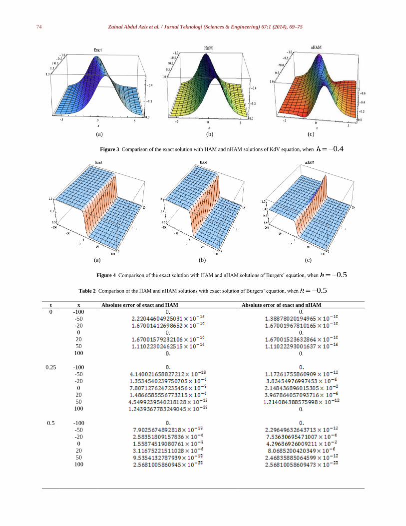
Table 2 Comparison of the HAM and nHAM solutions with exact solution of Burgers’ equation, when 0.5
Absolute error of exact and nHAM Absolute error of exact and HAM x t
0.
0.
0.
0.
0.
-100
-50
-20
0
20
50
100
0
0.
-100
-50
-20
0
20
50
100
0.25
-100
-50
-20
0
20
50
100
0.5

75 Zainal Abdul Aziz et al. / Jurnal Teknologi (Sciences & Engineering) 67:1 (2014), 69–75
Absolute error of exact and nHAM Absolute error of exact and HAM x t
0.
-100
-50
-20
0
20
50
100
0.75
0.
0.
-100
-50
-20
0
20
50
100
1
9.0 CONCLUSION
In this work, a comparative analysis of HAM and nHAM
methods is implemented for the KdV and the Burgers’
equations. The results obtained by HAM and nHAM are
compared with the standard exact soliton solution of KdV and
Burgers’ equations and found to be in excellent agreement.
However, the HAM solution of these equations is observed to be
more accurate than the nHAM solution. We are of the opinion
that this observation ratifies Hassan and El-Tawil[20] and [21],
which states that the new technique of HAM, i.e. nHAM, is
more suitable to obtain approximate analytical solutions of some
initial value problems of high-order t-derivative (order n 2 )
of nonlinear partial differential equations. However the KdV
and Burgers’ equations are examples where the order n = 1 ,
and we have shown that the accuracy of HAM for these cases
are better than nHAM.
Acknowledgement
This research is partially funded by MOE FRGS Vot No.
R.J130000.7809.4F354.
References
[1] Ablowitz, M., and P. Clarkson. 1991. Solitons, Nonlinear Evolution
Equations and Inverse Scattering. Cambridge University Press.
[2] Drazin, P. G., and R. S. Johnson. 1996. Solitons: An Introduction.
Cambridge University Press.
[3] Hirota, R. 2004. The Direct Method in Soliton Theory. Cambridge
University Press.
[4] Liao, S. J. 1992. The Proposed Homotopy Analysis Technique for the
Solution of Nonlinear Problems [PhD. Thesis], Jiao University. [5] Liao, S., Ed. 2004. Beyond Perturbation: Introduction to the Homotopy
Analysis Method. Chapman and Hall, Boca Raton, Fla, USA.
[6] Abbasbandy, S. 2007. The Application of Homotopy Analysis Method
to Solve a Generalized Hirota-Satsuma Coupled KdV Equation.
Physics Letters A. 361(6): 478–483.
[7] Ayub, M., A. Rasheed, and T. Hayat. 2003. Exact Flow of a Third
Grade Fluid Past a Porous Plate Using Homotopy Analysis Method.
International Journal of Engineering Science. 41(18): 2091–2103. [8] Hayat, T., M. Khan, and M. Ayub. 2005. On Non-linear Flows with
Slip Boundary Condition. Zeitschrift für Angewandte Mathematik und
Physik. 56(6):1012–1029.
[9] Nazari, M., F. Salah, Z. A. Aziz, M. Nilashi. 2012. Approximate
Analytic Solution for the Kdv and Burger Equations with the
Homotopy Analysis. Journal of Applied Mathematics. Article ID
878349, 13 pages. [10] Aziz, Z. A., M. Nazari, F. Salah and D.L.C. Ching. 2012. Constant
Accelerated Flow for a Third-grade Fluid in a Porous Medium and a
Rotating Frame with the Homotopy Analysis Method. Mathematical
Problems in Engineering. Article ID 601917, 14 pages.
[11] Liao, S. and E. Magyari. 2006. Exponentially Decaying Boundary
Layers as Limiting Cases of Families of Algebraically Decaying Ones.
Zeitschrift für Angewandte Mathematik und Physik. 57(5): 777–792. [12] Liao, S. 2006. Series Solutions of Unsteady Boundary-layer Flows
Overa Stretching Flat Plate. Studies in Applied Mathematics. 117(3):
239–263.
[13] Liao, S.J. 2003. On the Analytic Solution of Magnetohydrodynamic
Flows of Non-Newtonian Fluids Over A Stretching Sheet. Journal of
Fluid Mechanics. 488(1): 189–212.
[14] Abbasbandy, S. 2006. The Application of Homotopy Analysis Method
to Nonlinear Equations Arising in Heat Transfer. Physics Letters A. 360(1): 109–113.
[15] Abbasbandy, S. 2007. HomotopyAnalysis Method for Heat Radiation
Equations. International Communications in Heat and Mass Transfer.
34(3): 380–387.
[16] Abbasbandy, S. and A. Shirzadi. 2011. A New Application of the
Homotopy Analysis Method: Solving the Sturm-Liouville Problems.
Communications in Nonlinear Science and Numerical Simulation.
16(1):112–126. [17] Sami Bataneh, A., M. S. M. Noorani and I. Hashim. 2008.
Approximate Solutions of Singular Two-point BVPs by Modified
Homotopy Analysis Method. Physics Letter A. 372: 4062–4066.
[18] Sami Bataneh, A., M. S. M. Noorani and I. Hashim. 2009. On a New
Reliable Modification of Homotopy Analysis Method.
Communications in Nonlinear Science and Numerical Simulation. 14:
409–423. [19] Sami Bataneh, A., M. S. M. Noorani and I. Hashim. 2009. Modified
Homotopy Analysis Method for Solving Systems of Second-order
BVPs. Communications in Nonlinear Science and Numerical
Simulation. 14: 430–442.
[20] Hassan, H. N., and M. A. El-Tawil. 2011. A New Technique of Using
Homotopy Analysis Method for Solving High-order Nonlinear
Differential Equations. Mathematical Methods in the Applied Sciences.
34(6): 728–742. [21] Hassan, H. N., and M. A. El-Tawil. 2012. A New Technique Of Using
Homotopy Analysis Method for Second Order Nonlinear Differential
Equations. Applied Mathematics and Computation. 219. 708–728.
[22] Ablowitz, M., and V. Segur. 1981. Solitons and the Inverse Scattering
Transform. Philadelphia, PA: SIAM.
[23] Ablowitz, M. and P. Clarkson.1991.Soliton, Nonlinear Evolution
Equation and Inverse Scattering. Cambridge University Press. [24] Crighton, D. G. 1995. Applications of KdV. Acta Applicandae
Mathematicae. 39: 39–67.
[25] Wazwaz, A. M. 2001. Construction of Solitary Wave Solution and
Rational Solutions for the Kdv Equation by Adomian Decomposition
Method.Chaos, Solitons and Fractal. 12(12): 2283–2293.