Approximate analytical solutions for solute transport in two-layer porous media

Transport in Porous Media 18: 65-85, 1995. 65 @ 1995 KluwerAcademic Publishers. Printed in the Netherlands.

Approximate Analytical Solutions for Solute Transport in Two-layer Porous Media*

E J. LEIJ and M. TH. VAN G E N U C H T E N U.S. Salinity Laboratory, USDA-ARS, 4500 Glenwood Drive, Riverside, CA 92501, U.S.A.

(Received: 18 January 1994; in final form: 10 May 1994)

Abstract. Mathematical models for transport in layered media are important for investigating how restricting layers affect rates of solute migration in soil profiles; they may also improve the analysis of solute displacement experiments. This study reports an (approximate) analytical solution for solute transport during steady-state flow in a two-layer medium requiring continuity of solute fluxes and resident concentrations at the interface. The solutions were derived with Laplace transformations making use of the binomial theorem. Results based on this solution were found to be in relatively good agreement with those obtained using numerical inversion of the Laplace transform. An expression for the flux-averaged concentration in the second layer was also obtained. Zero- and first-order approximations for the solute distribution in the second layer were derived for a thin first layer representing a water film or crust on top of the medium. These thin-layer approximations did not perform as well as the 'binomial' solution, except for the first-order approximation when the Peclet number, P, of the first layer, was low (P < 5). Results of this study indicate that the ordering of two layers will affect the predicted breakthrough curves at the outlet of the medium. The two-layer solution was used to illustrate the effects of dispersion in the inlet or outlet reservoirs using previously published data on apparatus-induced dispersion.

Key words: Solute transport, composite media, boundary conditions.

1. I n t r o d u c t i o n

Knowledge of solute transport through composi te or layered porous media is o f impor tance to better manage and describe the movemen t of chemicals in natural and artificial media. Interest in porous media transport is increasingly mot ivated

by concerns over the presence of a wide variety of chemical substances and wastes

in the subsurface environment . Mathematical models are necessary to assess the fate and m o v e m e n t of such chemicals.

Porous media are se ldom homogeneous and the transport properties of these

media will vary spatially and somet imes also temporally. Accurate mathemat ical analyses of transport in heterogeneous media are not easily carried out. However , formulat ion and mathemat ica l solution of the transport problem becomes possible if the med ium is assumed, somewhat simplistically, to be composed of a series of homogeneous layers. In soil science, composi te media have been used for representing stratified soil profiles in which horizons parallel to the soil surface

* The U.S. Government fight to retain a non-exclusive, royalty free licence in and to any copyright is acknowledged.

66 E J. LEIJ AND M. TH. VAN GENUCHTEN

form layers with different transport properties (Selim et al., 1977; Jacobsen et al., 1991). Nakayama et al. (1984) investigated the movement of radionuclides through a medium consisting of soil and granite. Layered media are often also created artificially to slow down or prevent chemical movement (clay liners).

Solute transport in porous media has traditionally been described with the deter- ministic advection-dispersion equation (ADE). Taylor (1953) demonstrated that the concept of dispersion, although physically quite different, is mathematically equiv- alent to Fickian diffusion for sufficiently large travel times. This does not always hold and dispersion will not follow traditional Fickian behavior near interfaces or boundaries, the use of a macroscopically constant dispersion coefficient is formally incorrect in such cases (Dagan and Bresler, 1985). Given the lack of alternative concepts of dispersion that can be conveniently used in relatively simple transport models, the ADE with distinct dispersion coefficients for each layer still seems attractive for modeling transport in composite media (Parker and van Genuchten, 1985). This is particularly true if the ADE is used in a consistent manner for data analysis or prediction purposes.

Mathematical descriptions of transport in layered media have also been employed to evaluate the appropriateness of inlet and outlet boundary conditions for homogeneous systems. For example, the boundary conditions suggested by Danck- werts (1953) follow from the more general conditions formulated by Wehner and Wilhelm (1956) by ignoring dispersion in the infiuent and effluent reservoirs. These assumptions can most easily be evaluated if appropriate mathematical solutions and parameter values are available for multi-layer transport. Porous media may be viewed as assemblies of 'independent' homogeneous layers. Such a concept has been helpful for formulating interface conditions for transport during steady flow perpendicular to the layers. For each layer, a first- or third-type condition is used for the upper boundary while the lower boundary condition is formulated by means of a zero gradient at the outlet or at infinity (e.g., Shamir and Harleman, 1967; A1-Niami and Rushton, 1979). This approach usually assumes that the influent concentration for the second layer follows directly from the concentration predicted at the outlet of the first layer. The concentration in any layer is now independent of the transport properties of all downstream layers; the mathematical solution procedure is then greatly simplified while the problem of formulating more complicated alternative interface conditions is circumvented.

An alternative condition at the interface, first used by Wehner and Wilhelm (1956), requires that both the solute flux and the concentration be continuous. Conditions of this type have been routinely used for heat flow problems involving composite media (Carslaw and Jaeger, 1959; Ozi~ik, 1980). Given the similar nature of the ADE and the diffusion or heat flow equation, it is intuitively appealing to formulate the interface condition for solute transport in this manner although we realize that no 'perfect' boundary conditions exist. Despite additional mathematical complications, several authors seem to prefer the combined interface conditions (e.g., van der Laan, 1958; Kreft, 1981b; Barry and Parker, 1987). Such conditions

APPROXIMATE ANALYTICAL SOLUTIONS FOR SOLUTE TRANSPORT 67

may also be appropriate for the inlet and outlet conditions of homogeneous porous media. Unfortunately, the concentration in influent and effluent reservoirs can typically not be accurately characterized as a function of time and/or position except for some special cases (Novakowski, 1992b).

Analytical solutions for one-dimensional transport in composite media are often derived with Laplace transforms (Carslaw and Jaeger, 1959) and sometimes with Green's functions, adjoint solution techniques, and finite integral transforms (Mikhailov and Ozi~ik, 1984). Solutions can be readily obtained for an arbitrary number of layers if each layer is viewed as being an effectively semi-infinite medium. The use of Laplace transforms becomes more complicated if the concentration of a certain upstream layer depends on properties of its downstream layers. This situation arises when both concentration and solute flux are required to be continuous at the interfaces. The resulting mathematical problem may be simplified by considering only two layers, or by limiting the solution to only the steady-state case (Kreft, 1981b). Frequently, the Laplace transform has been inverted numerically. For instance, Barry and Parker (1987) obtained flux-averaged concentrations in this manner, while Leij et al. (1991) used this approach to predict volume- averaged concentrations. Novakowski (1992a) similarly used numerical inversion to predict concentrations in the porous medium as well as in the upstream and downstream reservoirs. The two- or multi-layered transport problem can also be conveniently analyzed by means of transfer functions or temporal moments (cf. Kreft, 1981a; Barry and Parker, 1987). Transfer function in the regular time domain (i.e., travel time distributions) could be obtained experimentally, or mathematically by using a Dirac input boundary conditions and Duhamel's theorem. Jury and Utermann (1992) formulated a joint probability density function for the travel time through a two-layer soil by assuming that the travel times in the individual layers were either perfectly correlated or independent. These authors explored the influence of transverse variations in transport due to different paths for water flow.

To the best of our knowledge, no explicit solutions are available for the ADE requiring simultaneous continuity in flux and concentration at the interfaces. The objective of this study is to derive an (approximate) solution for transport in a two-layer medium during steady flow using the method of Laplace transforms. The solution will be evaluated through comparisons with results obtained by numerical inversion of the Laplace transform. Alternative approximate solutions may be appropriate in some cases. An approximation for the case of a thin first layer will be presented. Several examples of resident concentration profiles versus position or time, and flux-averaged concentration distributions versus time, will be presented for cases where the two-layer solution may clarify certain theoretical and experimental aspects of solute transport in layered porous media.

68 F.J. LED AND M. TH. VAN GENUCHTEN

2. Problem Formulation

The porous medium is assumed to consist of two homogeneous layers subject to steady water flow perpendicular to the layer interface. The transport and flow properties of both layers are macroscopically uniform in time and space, while the ADE is assumed to describe transport in each layer. These simplifying assumptions are made to facilitate the derivation of an analytical solution. The governing transport equations are

0C1 02C1 0C1 O---i- = D10x----- T -- l]l-~-x , 0 ~ x ~ L, t > O, (I)

0•_2 oQ2C2 ~ x 2 - - = D 2 ~ ' ~ x 2 - - P 2 , L ~< z < o% t > 0, (2)

where C is the volume-averaged (resident) solute concentration, t is time, x is distance in the direction of flow, L is the position of the interface, D is the dispersion coefficient, u is the mean pore-water velocity, while the subscripts 1 and 2 refer to the first and second layer, respectively. The second layer is chosen to be semi- infinite for a convenient formulation of the outlet condition, this formulation can also be applied to finite systems.

The partial differential equations are augmented by a zero initial condition, a third-type inlet condition involving a step input, first- and third-type interface conditions, and a zero gradient at infinity as follows

C~(x, o) = c2(~, o) = o, (3)

ul = D 0C1 C0 a=O- ( U1C1- 1-'~--X ) x=O+' (4)

C1 Ix=L- -~- C2lw=L+, (5)

D OC,) (02v2C 2 02D2~_~) , ( OlplCI-O1 1-~z ] ]z=L - = -- ~=L+ (6)

0 c 2 ~ - ~ = o, (7)

where 0 denotes the volumetric water content and Co is the concentration of the influent solution at z = 0. As previously stated, conditions (4) and (7) are approximate because of difficulties to characterize the concentration in the influent and effluent regions.

The third- or flux-type condition is selected on physical grounds to ensure mass conservation whereas the first- or concentration-type condition is invoked on intuitive grounds (Kreft, 1981b). A combined first- and third-type condition at the


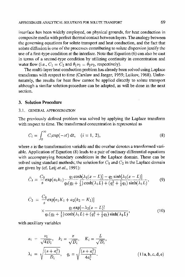
interface has been widely employed, on physical grounds, for heat conduction in composite media with perfect thermal contact between layers. The analogy between the governing equations for solute transport and heat conduction, and the fact that solute diffusion is one of the processes contributing to solute dispersion justify the use of a first-type condition at the interface. Note that Equation (6) can also be cast in terms of a second-type condition by utilizing continuity in concentration and water flow (i.e., C1 -- C2 and OlP 1 --~ 02/22, respectively).

The multi-layer heat conduction problem has already been solved using Laplace transforms with respect to time (Carslaw and Jaeger, 1959; Luikov, 1968). Unfor- tunately, the results for heat flow cannot be applied directly to solute transport although a similar solution procedure can be adapted, as will be done in the next section.

3. Solution Procedure

3.1. GENERAL APPROXIMATION

The previously defined problem was solved by applying the Laplace transform with respect to time. The transformed concentration is represented as

/5 Ci = Ciexp(-st) dt, (i = 1, 2), (8)

where s is the transformation variable and the overbar denotes a transformed variable. Application of Equation (8) leads to a pair of ordinary differential equations with accompanying boundary conditions in the Laplace domain. These can be solved using standard methods; the solution for C1 and C2 in the Laplace domain are given by (cf. Leij et al., 1991):

- - [ )C~ ql cosh[~l(X - L)] - q2 sinh[)q(x - L)] (9) ---- 1 s ql(q2 + 1) cosh (~ l 5 ) + (q2 .~ gq2)sinh()qL) '

C2 C~ + a2(k2 - K2)] 8

ql exp[-.~2(x -- L)] • ql(q2 + �89 cosh(,~,L) + (q2 + �89 sinh()qL)'

with auxiliary variables

(10)

ui x L a i - 4v/-g-~, k i - x / - - ~ , K i -

r k '

,~i = V/-~+a 2) i ( s + a 2 ) Di ' qi = 4a 2 ( l l a , b, c ,d ,e)


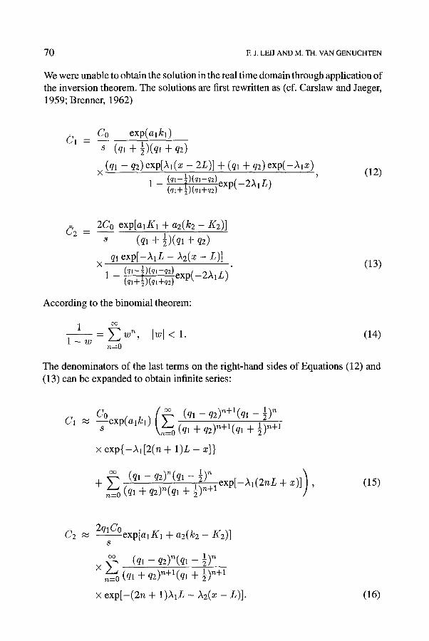
We were unable to obtain the solution in the real time domain through application of the inversion theorem. The solutions are first rewritten as (cf. Carslaw and Jaeger, 1959; Brenner, 1962)

01 Co exp(alkl) (ql + 1)(ql + q2)

(ql - q2) exp[Al(X - 2L)] + (ql + q2) exp(-AlX) (ql--~)(ql--q2) / ,-~. r'~

1 - (ql+ l)(qlTq2) exp~,--ZAl~) (12)

0 2 - - 2Co exp[alK1 + a2(k2 - K2)]

8 (ql + 21-)(ql -4- q2)

ql exp[-A1L- A2(x- L)] X

(ql--�89 " ~ " 1 ' ' " 1 - (ql+ l)(ql+q2) e x p k - - Z A l ~ )

(13)

According to the binomial theorem:

1 oO

l _ w - ~ w '~, I w l < l . (14) n~O

The denominators of the last terms on the right-hand sides of Equations (12) and (13) can be expanded to obtain infinite series:

Coexp(glkl) (n~= 0 ( g - - l - - q ~ ~ - - ! 2 ~ l ( q l - q2)n+l(ql-1)n

• exp{-Al[2(n + 1)L - x])

n 1 n ) (ql - q2) (ql - g) exp[-Al(2nL + x)]

+ (~11 -_t_- q2) n (q----~ -_k- }) n--71 (15)

C2 2qlC~ + a2(k2- K2)] 8

c~ (ql -- q2)n(ql -- 1)n • E (qi + 7 2 ; ; v g + )n+i

n=0

• exp[-(2n + 1)ALL - A2(x - L)]. (16)


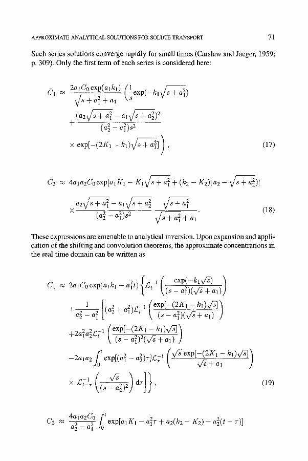
Such series solutions converge rapidly for small times (Carslaw and Jaeger, 1959; p. 309). Only the first term of each series is considered here:

2alCoexp(alkl) ( ! e x p ( _ k l v / S +a2) ~ f s + a2 + al

(a2v/7 + al 2 - alV/S + a]) 2 + ( a 2 -

x exp[-(2K1 -/~1)~1 '~, \

,/ (17)

C2 ~ 4a la2Coexp [a l t (1 - I (1 r -Jr- a 2 Jr (/r -/s ~/8 + a2)]

a2 ~//,s q- al 2 -- al Cs -'k a 2 V/7 -k al 2 x (18) a2)8 2 r + a 2 + al

These expressions are amenable to analytical inversion. Upon expansion and application of the shifting and convolution theorems, the approximate concentrations in the real time domain can be written as

C1 2a~Coexp(alkl-azt){f~tl ((sexp(-klVG)- ~ -a2)(x/~+al)J 1 [ (exp[__-(2Sl .~ kl)V~_ .'~

-}-a 2 - a 2 ,.(a2 q- a2) 'gtl \ (s - al2)(v'~ -k al) J

( exp[__-( 21(1 -- _k_l )v/} -] "] q-2al2a2Ctl \ (8 -- a~)2(X/~ + al) J

-2ala2 fot eXp[(a2 - a2)r]s ( v/~ exp[-(2Kl - kI )x/~ ) -~----+-a-1

(19)

4ala2Co fot C2 ~ -~- -~ exp[alK1 - a)r + a2(k2 - K2) - a~(t - 7-)] a 2 -- a 1

72

X

E J. LED AND M. TH. VAN GENUCHTEN

a~a2s ( (s exp(-Klv~) qt_ : ~ T a a ) ) ]

{ ~ e~p(-/r,~)

X / : t - r S -- a 2

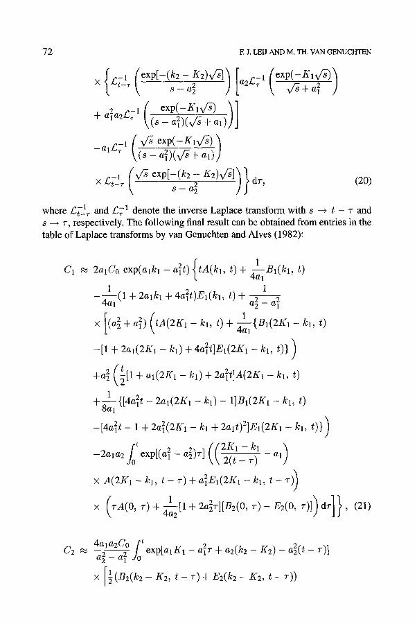
where - 1 s and s denote the inverse Laplace transform with s ~ t - ~- and s ~ v, respectively. The following final result can be obtained from entries in the table of Laplace transforms by van Genuchten and Alves (1982):

C1 2alCo exp(alkl -a2t) {tA(kl, t) + ~---~lBl(hl, t) 1

1 ( l q- 2 a l k l q- 4a2t)El(kl, t) q- a2 a----~l 4al

x [(a2 + a~) (tA(2Kl - kl, t) + ~---~l {Bl(2Kl - kl, t)

-[1 q- 2a,(2K1 - kl) q- 4a~t]El(2K1 - k l , t)} )

+a~ (211 + a1(2K1- kl) + 2a2t]Z(2K1- kl, t)

+8-~1 {[4aZt - 2a,(2tQ - k , ) - 1]Bff2IQ- kt, t)

-[4aZt - 1 + 2a12(ZK1- k, + 2alt)ZlE,(2K1- kl, t)})

-2ala2 foteXp[(a2 - a~)r] ((21(1 -- k___l \ \ 2(t - 7-) a l)

x A(2K1 - kl, t - 7-) + a2EI(2K1 - kl, t - v))

1 • (vA(0, 7-)+ ~a2[1 +2aZr][B2(0, T)-E2(0 , v)])d't-]}, (21)

Ca 4al a2Co ~o t -~-~---~ exp[a lK1 - a27" + a2(k2 - !(2) - a2(t - 7-)] a 2 - - a 1

• 1~ (.~(k~- u~, t - ~-)+ E~(k:- K~, t - ~-))


ala2 rn /,~ x a2(l+a2v)Z(K1, r ) + - 7 - k ~ I ( J X , , r)

- ( 5 + 2algl + 4a2r)EI(K1, r)] )

--al (41--BI(K1, 7-)+ 1(3 + 2alK1 + 4a217-)

• 7-)- alT-A(l(1, 7-))

x ( A ( k 2 - K2, t - r )+ 2 [ B 2 ( k 2 - K2, t -

/ J

,9-

(22)

where

A(k, t ) = ~ e x p (23)

Bi(k, t) = exp(a2t - aik) erfc (k - 2a#) 7/-g

(24)

El(k, t) : exp(a2t + aik) effc / ( k + 2a# "~

\ (25)

The integrals appearing in these solutions were evaluated with the help of Gauss- Chebyshev quadrature (Carnahan et al., 1969) whereas the subroutine EXF (van Genuchten and Alves, 1982) was used to obtain the product of exponential and complementary error functions. Note that the two-layer solutions diverge when the properties of both layers are similar (al = a2); the simpler homogeneous (one-layer) solution should then be used.

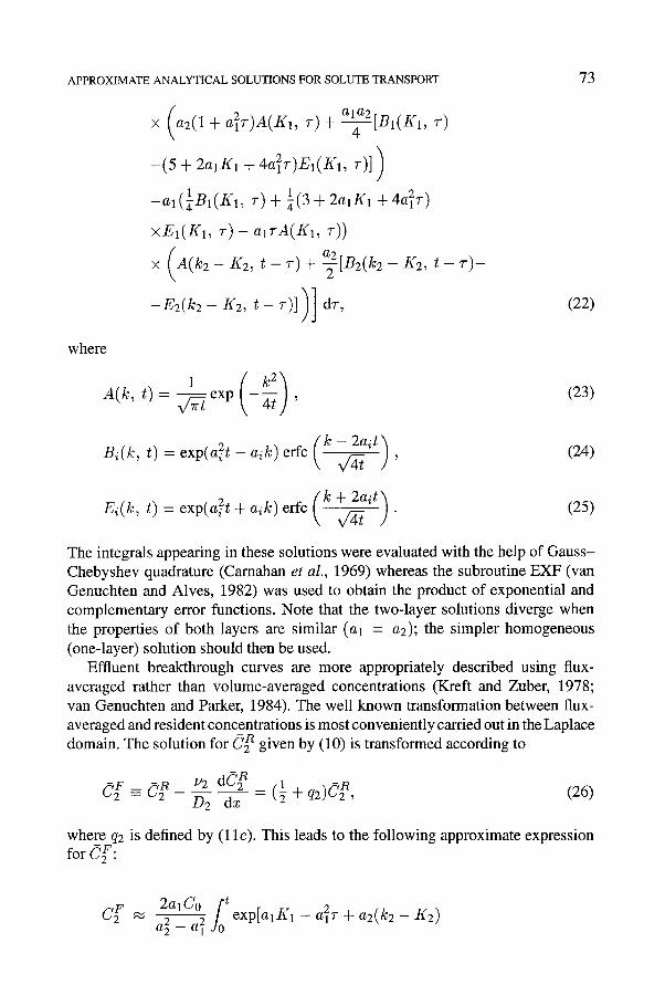
Effluent breakthrough curves are more appropriately described using flux- averaged rather than volume-averaged concentrations (Kreft and Zuber, 1978; van Genuchten and Parker, 1984). The well known transformation between flux- averaged and resident concentrations is most conveniently carried out in the Laplace domain. The solution for C2 R given by (10) is transformed according to

- d G 1 - R D2 dx - (3 + q2)C2 ' (26)

where q2 is defined by (1 le). This leads to the following approximate expression for C2F:

2alCo ~oo t C2F "~ 7g---7-2 exp[alI(1 - a2"r + a2(k2 - K2) a 2 - a 1

74 F.J. LEIJ AND M. TH. VAN GENUCHTEN

( ( e x p [ - (_k2__-__K2)v/~ ] - r ) ] \ _a2 )

, %

exp(- / (1 x/~) ~ • [~-1 ( ( a 2 - a l V ~ ) ~ - a l ]

( ex (- K, 1 + • r 1 \ (a2a2 - a'a~v/-d)(s - - ~ 7 - a l ) / ]

s

( - alv '~) e x p ( - K l v G) ~ ~ dr. X ~-.r 1 ~ a 2 ( 8 ( 8 _ a 2 ) ( v @ + a l ) ,] J (27)

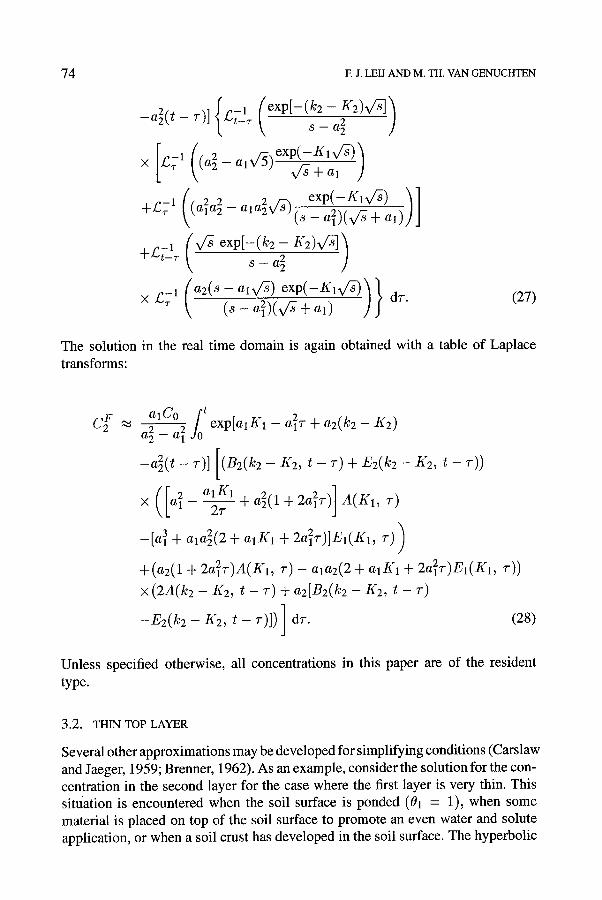
The solution in the real time domain is again obtained with a table of Laplace transforms:

a l Co frO t 2"----2 exp[alI(1 - a~r + a2(k2 -- K2) a 2 - a 1

-a29(t- 7-)] ](B2(k2 - K2, t - r) + E2(k2 - I(2, t - 7-))

• 2 _ alK12___~_ + a22(1 + 2a~r)]A(Kl, r)

+ ala2(2 + alK1 + 2a2r)]E,(K1, r) ) ~ ~a~

+(a2(1 + 2a21r)A(K1, r) - ala2(2 + alK1 + 2 a 2 r ) E l ( K l , v))

x (2A(k2 - 1(2, t - r) + a2[B2(k2 - K2, t - r)

- E i ( k 2 -- K2, t -- r ) ] ) / dr. (28) J

Unless specified otherwise, all concentrations in this paper are of the resident type.

3.2. THIN TOP LAYER

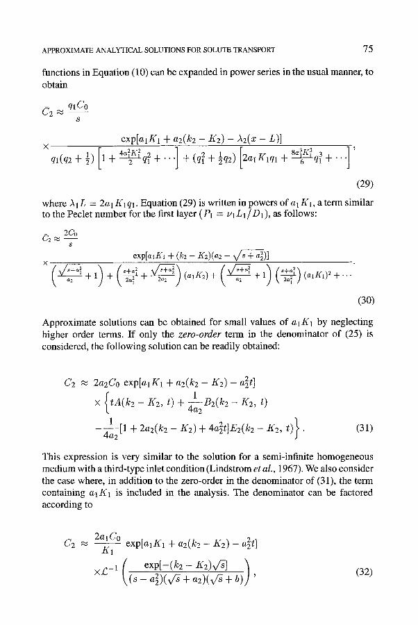
Several other approximations may be developed for simplifying conditions (Carslaw and Jaeger, 1959; Brenner, 1962). As an example, consider the solution for the concentration in the second layer for the case where the first layer is very thin. This situation is encountered when the soil surface is ponded (01 = 1), when some material is placed on top of the soil surface to promote an even water and solute application, or when a soil crust has developed in the soil surface. The hyperbolic


functions in Equation (10) can be expanded in power series in the usual manner, to obtain

C2 ~ ql Co 8

exp[alK1 + a2(k2 -- K2) - ,~2(X - - L)] • I [ ] ql(q2+ 1) 1 + 2 q l + " " +(q12+�89 2alKlql+ 6 q l + " " 2

(29)

where )qL = 2alKlql. Equation (29) is written in powers of alKl, a term similar to the Peclet number for the first layer (/1 = u~L1/D1), as follows:

62 ,~ 2Co s

x exp[alK~ + (kz - Kz)(a2 - V ~ a~)]

+ 1 + k 2,~ + 2a2 J \ ~2 + 1 ~ 2~ ] ( a 1 K 1 ) 2 + " '

(30)

Approximate solutions can be obtained for small values of alK1 by neglecting higher order terms. If only the zero-order term in the denominator of (25) is considered, the following solution can be readily obtained:

C2 2a2C0 exp[alKl + a2(k2 - K2) - a2t]

x I tA (k2 - K2, t )+ 4 - ~ B 2 ( k 2 - t(2, t)

- ~ 1 [1 + 2a2(k2 - I ( 2 ) + 4a2t]E2(k2 - K2, t)~. 4a2 J

(31)

This expression is very similar to the solution for a semi-infinite homogeneous medium with a third-type inlet condition (Lindstrom et al., 1967). We also consider the case where, in addition to the zero-order in the denominator of (31), the term containing alK1 is included in the analysis. The denominator can be factored according to

C2 "~ 2al Co - - exp[alK1 + a2(k2 - K2) - a~t]

K1

( exp[-(k2 - t (2)v '~ ) (32)


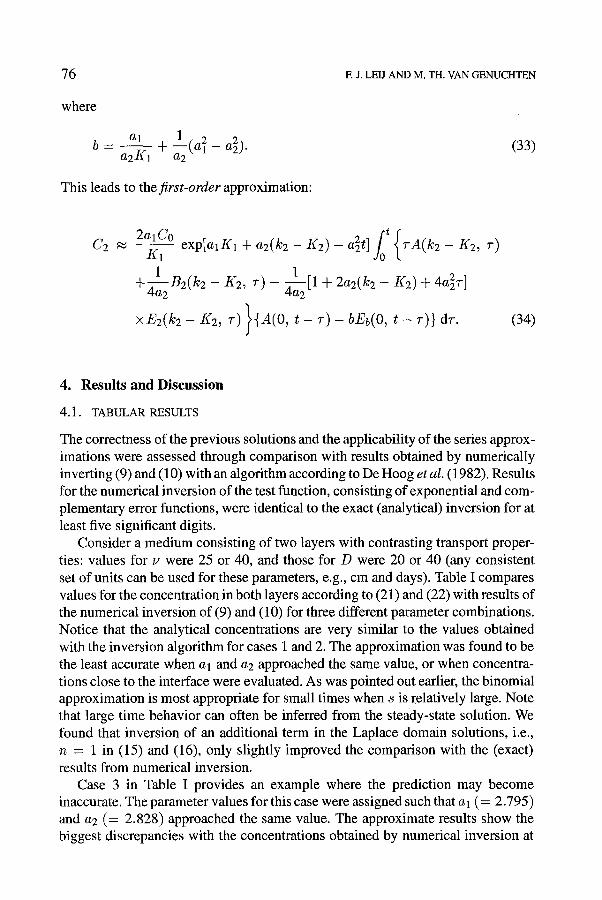
where

a l l b_ .2K +

This leads to thefirst-order approximation:

(33)

C2 2a l C_______~o

exp[alK1 + a 2 ( k 2 - 1 ( 2 ) - a2t] r]at (~7-n(k2- K2, 7-) K1

+ B2(ke - K2, 7-) - [1 + 2az(k2 - K2) + 4a 7-]

• - K2, 7-) ~{A(0, t - 7-) - bEb(O, t - 7-)} dr. )

(34)

4. Results and Discussion

4.1. TABULAR RESULTS

The correctness of the previous solutions and the applicability of the series approximations were assessed through comparison with results obtained by numerically inverting (9) and (10) with an algorithm according to De Hoog etal. (1982). Results for the numerical inversion of the test function, consisting of exponential and complementary error functions, were identical to the exact (analytical) inversion for at least five significant digits.

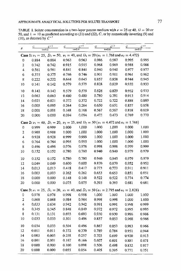
Consider a medium consisting of two layers with contrasting transport properties: values for v were 25 or 40, and those for D were 20 or 40 (any consistent set of units can be used for these parameters, e.g., cm and days). Table I compares values for the concentration in both layers according to (21) and (22) with results of the numerical inversion of (9) and (10) for three different parameter combinations. Notice that the analytical concentrations are very similar to the values obtained with the inversion algorithm for cases 1 and 2. The approximation was found to be the least accurate when al and a2 approached the same value, or when concentrations close to the interface were evaluated. As was pointed out earlier, the binomial approximation is most appropriate for small times w h e n , is relatively large. Note that large time behavior can often be inferred from the steady-state solution. We found that inversion of an additional term in the Laplace domain solutions, i.e., n = 1 in (15) and (16), only slightly improved the comparison with the (exact) results from numerical inversion.

Case 3 in Table I provides an example where the prediction may become inaccurate. The parameter values for this case were assigned such that al (= 2.795) and a2 (= 2.828) approached the same value. The approximate results show the biggest discrepancies with the concentrations obtained by numerical inversion at

APPROXIMATE ANALYTICAL SOLUTIONS FOR SOLUTE TRANSPORT

TABLE I. Solute concentration in a two-layer porous medium with v = 25 or 40, D = 20 or 50, and L = 10 as predicted according to (21) and (22), G, or by numerically inverting (9) and (10), as denoted by l ; - i

77

G' z2 - l G s G' s G' L - l X t = 0 , 2 t = 0 . 4 t = 0 . 6 t = 0 . 8

Case 1: vx = 25, D1 = 50, u2 = 40, and D2 = 20 (al = 1.768 and a2 = 4.472)

0 0.884 0.884 0.963 0.963 0.986 0.987 0.995 0.995

2 0.742 0.742 0.915 0.915 0.968 0.969 0.988 0.988

4 0.561 0.561 0.841 0.841 0.940 0.940 0.977 0.977

6 0.375 0.375 0.746 0.746 0.901 0.901 0.961 0.962

8 0.222 0.222 0.644 0.645 0.857 0.858 0.944 0.945

10 0.141 0.142 0.579 0.579 0.828 0.829 0.932 0.933

10 0.142 0.142 0.579 0.579 0.828 0.829 0.932 0.933

12 0.063 0.063 0.480 0.480 0.780 0.781 0.913 0.914

14 0.021 0.021 0.372 0.372 0.722 0.722 0.888 0.889

16 0.005 0.005 0.264 0.264 0.650 0.651 0.857 0.858

18 0.001 0.001 0.168 0.168 0.567 0.567 0.818 0.819

20 0.000 0.000 0.094 0.094 0.473 0.473 0.769 0.770

Case 2: Vl = 40, DI = 20, v2 = 25, and D2 = 50 (al = 4.472 and a2 --- 1.768)

0 0.999 0.999 1.000 1.000 1.000 1.000 1.000 1.000

2 0.988 0.988 1.000 1.000 1.000 1.000 1.000 1.000

4 0.928 0.928 0.999 0.999 1.000 1.000 1.000 1.000

6 0.764 0.764 0.995 0.995 1.000 1.000 1.000 1.000

8 0.496 0.496 0.976 0.976 0.998 0.998 0.999 0.999

10 0.152 0.152 0.780 0.780 0.940 0.940 0.979 0.979

10 0.152 0.152 0.780 0.780 0.940 0.940 0.979 0.979

12 0.049 0.049 0.600 0.600 0.870 0.870 0.952 0.952

14 0.013 0.013 0.418 0.417 0.773 0.773 0.911 0.911

16 0.003 0.003 0.262 0.262 0.653 0.653 0.851 0.851

18 0.000 0.000 0.148 0.148 0.522 0.522 0.774 0.774

20 0.000 0.000 0.075 0.075 0.393 0.393 0.681 0.681

Case 3:/}1 = 25, D~ = 20, v2 = 40, and D2 = 50 (al = 2.795 and a2 = 2.828)

0 0.978 0.978 0.998 0.998 1.000 1.000 1.000 1.000

2 0.868 0.868 0.984 0.984 0.998 0.998 1.000 1.000

4 0.633 0.634 0.942 0.942 0.991 0.991 0.998 0.999

6 0.345 0.345 0.848 0.849 0.972 0.972 0.995 0.995

8 0.131 0.131 0.693 0.693 0.930 0.930 0.986 0.986

10 0.033 0.033 0.501 0.496 0.857 0.853 0.968 0.966

10 0.034 0.033 0.504 0.496 0.867 0.853 0.983 0.966

12 0.011 0.011 0.372 0.370 0.789 0.784 0.951 0.944

14 0.003 0.003 0.258 0.257 0.703 0.699 0.920 0.913

16 0.001 0.001 0.167 0.166 0.607 0.601 0.881 0.871

18 0.000 0.000 0.100 0.098 0.506 0.498 0.832 0.817

20 0.000 0.000 0.055 0.054 0.405 0.395 0.771 0.751

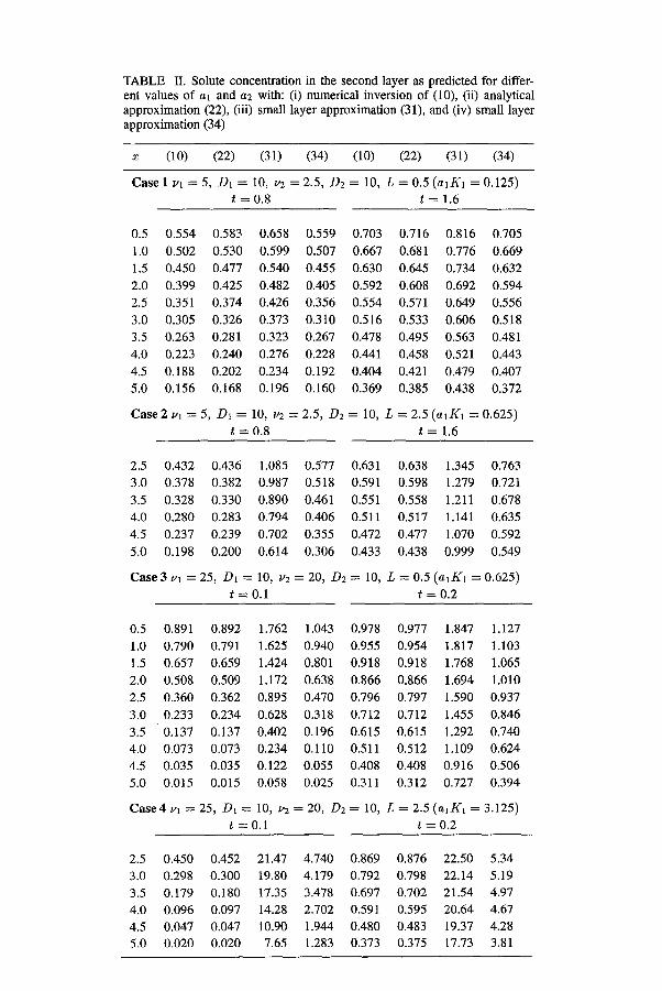
TABLE II. Solute concentration in the second layer as predicted for different values of al and a2 with: (i) numerical inversion of (10), (ii) analytical approximation (22), (iii) small layer approximation (31), and (iv) small layer approximation (34)

x (10) (22) (31) (34) (10) (22) (31) (34)

Case 1 vl = 5, D1 = 10, /32 = 2.5, D2 = 10, L = 0.5 ( a l / ( l = 0.125) t = 0.8 t = 1.6

0.5 0.554 0.583 0.658 0.559 0.703 0.716 0.816 0.705

1.0 0.502 0.530 0.599 0.507 0.667 0.681 0.776 0.669

1.5 0.450 0.477 0.540 0.455 0.630 0.645 0.734 0.632

2.0 0.399 0.425 0.482 0.405 0.592 0.608 0.692 0.594

2.5 0.351 0.374 0.426 0.356 0.554 0.571 0.649 0.556

3.0 0.305 0.326 0.373 0.310 0.516 0.533 0.606 0.518

3.5 0.263 0.281 0.323 0.267 0.478 0.495 0.563 0.481

4.0 0.223 0.240 0.276 0.228 0.441 0.458 0.521 0.443

4.5 0.188 0.202 0.234 0.192 0.404 0.421 0.479 0.407

5.0 0.156 0.168 0.196 0.160 0.369 0.385 0.438 0.372

C a s e 2 vl = 5, D1 = 10, v2 = 2.5, D2 -- 10, L = 2.5 (aaK1 = 0.625)

t = 0 . 8 t = l . 6

2.5 0.432 0.436 1.085 0.577 0.631 0.638 1.345 0.763

3.0 0.378 0.382 0.987 0.518 0.591 0.598 1.279 0.721

3.5 0.328 0.330 0.890 0.461 0.551 0.558 1.211 0.678

4.0 0.280 0.283 0.794 0.406 0.511 0.517 1.141 0.635

4.5 0.237 0.239 0.702 0.355 0.472 0.477 1.070 0.592

5.0 0.198 0.200 0.614 0.306 0.433 0.438 0.999 0.549

C a s e 3 Ul = 25, D1 ---=- 10, /32 = 20, D2 ----- 10, L = 0.5 (alK1 = 0.625)

t = 0 . 1 t = 0 . 2

0.5 0.891

1.0 0.790

1.5 0.657

2.0 0.508

2.5 0.360

3.0 0.233

3.5 0.137

4.0 0.073

4.5 0.035

5.0 0.015

Case 4/-'1 :

0.892 1.762 1.043 0.978 0.977 1.847 1.127

0.791 1.625 0.940 0.955 0.954 1.817 1.103

0.659 1.424 0.801 0.918 0.918 1.768 1.065

0.509 1.172 0.638 0.866 0.866 1.694 1.010

0.362 0.895 0.470 0.796 0.797 1.590 0.937

0.234 0.628 0.318 0.712 0.712 1.455 0.846

0.137 0.402 0.196 0.615 0.615 1.292 0.740

0.073 0.234 0.I10 0.511 0.512 1.109 0.624

0.035 0.122 0.055 0.408 0.408 0.916 0.506

0.015 0.058 0.025 0.311 0.312 0.727 0.394

25, DL = 10, v2 = 20, D2 = 10, L = 2.5 (alK1 = 3.125)

t-----0.1 t = 0 . 2

2.5 0.450 0.452 21.47 4.740 0.869 0.876 22.50 5.34

3.0 0.298 0.300 19.80 4.179 0.792 0.798 22.14 5.19

3.5 0.179 0.180 17.35 3.478 0.697 0.702 21.54 4.97

4.0 0.096 0.097 14.28 2.702 0.591 0.595 20.64 4.67

4.5 0.047 0.047 10.90 1.944 0.480 0.483 19.37 4.28 5.0 0.020 0.020 7.65 1.283 0.373 0.375 17.73 3.81


or near the interface when the solute reaches the second layer. Inverting a second term for the series expression of C2 did not yield significantly different results.

Table II compares values for the concentration in the second layer predicted with (i) numerical inversion of (10), (ii) the binomial expansion according to (23), (iii) the zero-order approximation for small L, and (iv) the first-order approximation for small L. The usefulness of the approximations was again assessed by using the numerical inversion technique as the 'benchmark' method. Solute profiles are given for two values of t assuming a medium with a length typical of soil cores and using four different parameter sets. Case 1 involves a relatively thin first layer with fairly small values for al , a2, and L. The first-order thin-layer approximate solution (34) is most suitable for this case while approximation (22) performs relatively poor because of a low Peclet number,/91. Notice that zero-order approximation (31) is much less accurate. The same transport parameters as for case 1 were also used for case 2, except that both layers were now of equal length. Because of the increase in L, the short-layer approximations were found to be less accurate; conversely, the solutions according to (22) became more reliable. Case 3 of Table II involves a higher value for a I and again a smaller L such that alK1 is the same as for case 2. The results in Table II show that the relative errors associated with the first-order short-layer approximation are similar for cases 2 and 3 for both short- layer approximations. Finally, case 4 illustrates that the thin-layer approximations become progressively worse for larger a lK1.

4.2. G R A P H I C A L RESULTS

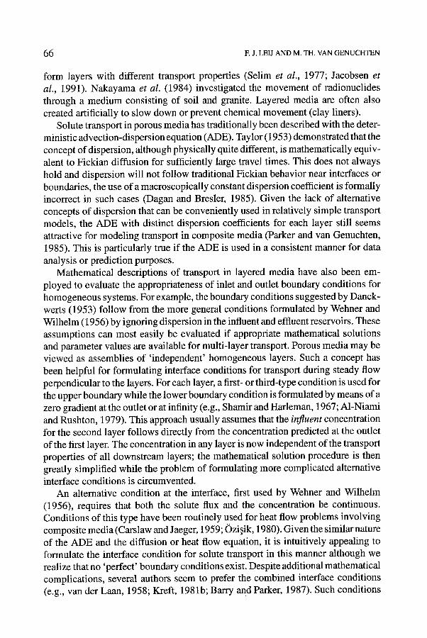
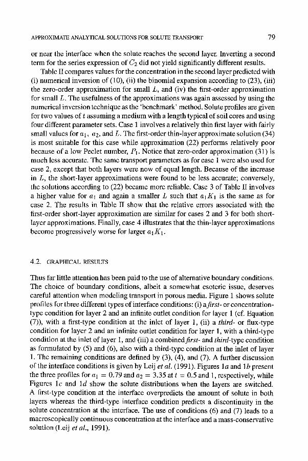
Thus far little attention has been paid to the use of altemative boundary conditions. The choice of boundary conditions, albeit a somewhat esoteric issue, deserves careful attention when modeling transport in porous media. Figure 1 shows solute profiles for three different types of interface conditions: (i) afirst- or concentration- type condition for layer 2 and an infinite outlet condition for layer 1 (cf. Equation (7)), with a first-type condition at the inlet of layer 1, (ii) a third- or flux-type condition for layer 2 and an infinite outlet condition for layer 1, with a third-type condition at the inlet of layer 1, and (iii) a combined first- and third-type condition as formulated by (5) and (6), also with a third-type condition at the inlet of layer 1. The remaining conditions are defined by (3), (4), and (7). A further discussion of the interface conditions is given by Leij et al. (1991). Figures la and lb present the three profiles for a 1 = 0.79 and az = 3.35 at t = 0.5 and 1, respectively, while Figures lc and ld show the solute distributions when the layers are switched. A first-type condition at the interface overpredicts the amount of solute in both layers whereas the third-type interface condition predicts a discontinuity in the solute concentration at the interface. The use of conditions (6) and (7) leads to a macroscopically continuous concentration at the interface and a mass-conservative solution (Leij et al., 1991).

8 0 E J. LEIJ AND M. TH. VAN GENUCHTEN

o o

1.0

0.8 ~

0.6 -

0.4 -

0.2 -

0 .0

�9 ~ ' t=05 '

v =101~ D =40 I " ~ . . ~ _

1.0

0.8 ~

o 0.6 r

0.2

0.0

' Jl t = 0 5 '

i ! ~ I

1 ~, , I Vz~lO =51:)2=40

b 5 & D= = 5 VI=I - _ �9 I �9 I , I

o

1.0

0.8

0.6

0.4

0.2

0 . 0

t

V, =iO ~ D I =40 i V,=15.~ D2= 5,

0 5 10 15 X

1.0

0 . 8 -

3 0.6

0.4

0.2

V==158 Dr=5 0 .0

20 0 5

---•, ,=," ' d

Vz=lO&02=40

10 15 20 X

. . . . . . . . . . . f i rs t th i rd f i rs t & th i rd

. . . . . . . . . . . f i rs t . . . . . . . . . th i rd

f i rs t & th i rd

Fig. 1. Solute profiles in a two-layer medium predicted using (i) a first-type, (ii) a third-type, and (iii) a first- and third-type interface condition with//1 = 10, Dt = 40, u2 = 15, and D2 = 5 at (a) t = 0.5, and (b) t = 1, and with Ul = 15, D] = 5, u2 = 10, and Dz = 40 at (c) t = 0.5, and (d) t = 1.

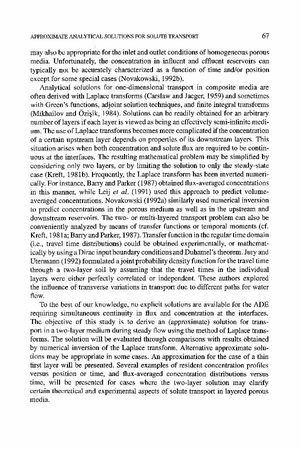
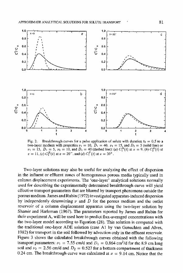
Knowledge of the time-dependent behavior of solutes in the subsurface is of interest for many practical problems where the concentration is observed or needs to be predicted at fixed positions. Figure 2 shows breakthrough curves, resulting from a solute pulse with duration 0.5, just before (x = 9) and after (z = 11) the interface, and at the outlet of the second layer (z = 20- ) , for the resident concentration calculated with (21) and (22). Also included are results for the flux- averaged concentration at the outlet of the second layer (x = 20 +) calculated with (28). The same parameters are used as for the example shown in Figure 1. Figure 2 may be used to examine how the ordering of the two layers affects a breakthrough curve. As expected, the curves at x = 9 and 11 are different when the layers are switched. However, notice that the curves in Figures 2c and 2d are also different at z -- 20 after the solute has traversed an equal distance in both layers. In contrast, for a medium consisting of two 'semi-infinite' layers it can be shown explicitly that the order of the semi-infinite layers does not affect the outlet concentration (Shamir and Harleman, 1967; Leij et al., 1991). This last finding for the mathematically semi-infinite first layer is a result of the assumption that properties of layer 2 will not influence the concentration of layer 1.

A P P R O X I M A T E A N A L Y T I C A L S O L U T I O N S FOR S O L U T E T R A N S P O R T ~ 81

o o

{e.,,,~

1.0

0.8

0.6

0 .4

0.2

0 . 0

x= 9, 1 i i

i t i

i t

0

o ej

i.O

O.B

0.6

0.4

0.2

0 . 0

' i i i

X:20- C

s S

r

1.0

0.8

0.6

0.4

0.2

0 .0

0

X=ll b

t ~

1 2 3

t

o o

1.0

0.8

0.6

0.4

0.2

0.0

• d

1 2 3 4

t

Fig. 2. Breakthrough curves for a pulse application of solute with duration to = 0.5 to a two-layer medium with properties Vl = 10, D1 = 40, v2 = 15, and D2 = 5 (solid line) or vl = 15, D] = 5, v2 = 10, and D2 = 40 (dashed line): (a) C~(t) at z = 9, (b) C~(t) at z = 11, (c) G~(t) atx = 20-, and(d) C~(t) atz = 20 +.

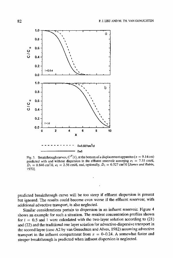
Two-layer solutions may also be useful for analyzing the effect of dispersion in the influent or effluent zones of homogeneous porous media typically used in column displacement experiments. The 'one-layer ' analytical solutions normally used for describing the experimentally determined breakthrough curve will yield effective transport parameters that are blurred by transport phenomena outside the porous medium. James and Rubin (1972) investigated apparatus-induced dispersion by independently determining v and D for the porous medium and the outlet reservoir of a column displacement apparatus using the two-layer solution by Shamir and Harleman (1967). The parameters reported by James and Rubin for their experiment A, will be used here to predict flux-averaged concentrations with the two-layer model according to Equation (28). This solution is compared with the traditional one-layer ADE solution (case A1 by van Genuchten and Alves, 1982) for transport in the soil fol lowed by advection only in the effluent reservoir. Figure 3 shows the calculated breakthrough curves obtained with the following transport parameters: ui = 7.55 cm/d and D1 = 0.864 cm2/d for the 8.9 cm long soil and u2 = 2.56 cm/d and D2 = 0.527 for a bot tom compartment of thickness 0.24 cm. The breakthrough curve was calculated at z = 9.14 cm. Notice that the


1.0

0 .8

o 0 .6 (3

0 0.4

0.2

0.0

1.0

0 ,8

o 0.6 0

t,.) 0.4

0.2

0.0

" 1 ,~, % �9 I " I I

1 =0.Sd "~% _

t=ld , I

2

I ~ I ~ I ~ J ~ 4 6 8 40

X

. . . . . . . . . . . D=O.527cm2/d

D=O

Fig. 3. Breakthrough curves, C F (~), at the bottom of a displacement apparatus (z = 9.14 cm) predicted with and without dispersion in the effluent reservoir assuming ul = 7.55 cm/d, D1 = 0.846 cm2/d, u2 ---- 2.56 cm/d, and, optionally, D2 = 0.527 cm2/d [James andRubin, 1972].

predicted breakthrough curve will be too steep if effluent dispersion is present but ignored. The results could become even worse if the effluent reservoir, with additional advective transport, is also neglected.

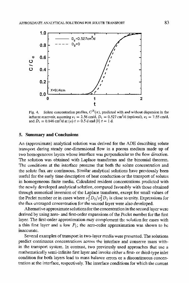
Similar considerations pertain to dispersion in an influent reservoir. Figure 4 shows an example for such a situation. The resident concentration profiles shown for t = 0.5 and 1 were calculated with the two-layer solution according to (21) and (22) and the traditional one layer solution for advective-dispersive transport in the second layer (case A2 by van Genuchten and Alves, 1982) assuming advective transport in the influent compartment from z = 0-0.24. A somewhat faster and steeper breakthrough is predicted when influent dispersion is neglected.


1.0 ~ ' I ~ *~ ,d , , , , , , l l ' ' ~ ' ~ -- D2 =0.527em2/d 0.8 D2=O /"

o 0.6 t/' (J

0 0.4

0.2 X=9.14cm M/g~ Stir'! , , 0.0

0 I 2 t

Fig. 4. Solute concentration profiles, CR(x) , predicted with and without dispersion in the influent reservoir, assuming ~q = 2.56 cm/d, D1 = 0.527 cm2/d (optional), u2 = 7.55 cm/d, and D2 = 0.846 crn2/d at (a) t = 0.5 d and (b) t = 1 d.

5. Summary and Conclusions

An (approximate) analytical solution was derived for the ADE describing solute transport during steady one-dimensional flow in a porous medium made up of two homogeneous layers whose interface was perpendicular to the flow direction. The solution was obtained with Laplace transforms and the binomial theorem. The conditions at the interface presume that both the solute concentration and the solute flux are continuous. Similar analytical solutions have previously been useful for the early time description of heat conduction or the transport of solutes in homogeneous finite media. Calculated resident concentrations predicted with the newly developed analytical solution, compared favorably with those obtained through numerical inversion of the Laplace transform, except for small values of the Peclet number or in cases where u~D2/uZD1 is close to unity. Expressions for the flux-averaged concentration for the second layer were also developed.

Alternative approximate solutions for the concentration in the second layer were derived by using zero- and first-order expansions of the Peclet number for the first layer. The first-order approximation may complement the solution for cases with a thin first layer and a low P1; the zer0-order approximation was shown to be inaccurate.

Several examples of transport in two-layer media were presented. The solutions predict continuous concentrations across the interface and conserve mass with- in the transport system. In contrast, two previously used approaches that use a mathematically semi-infinite first layer and invoke either a first- or third-type inlet condition for both layers lead to mass balance errors or a discontinuous concentration at the interface, respectively. The interface conditions for which the current


tration at the interface, respectively. The interface conditions for which the current

solutions were derived imply that the ordering of the layers will affect the breakthrough curve at the outlet of the medium. The utility of the two-layer solution for analyzing transport in the influent or effluent regions of laboratory columns was illustrated using experimental data pertaining to apparatus-induced dispersion.

Acknowledgments

We would like to thank John Knight for providing a copy of the numerical inversion program according to the De Hoog method, as well as Ed Sudicky for supplying us a version modif ied by Chris Neville.

References

A1-Niami, A. N. S. and Rushton, K. R., 1979, Dispersion in stratified porous media: analytical solutions, Water Resour. Res. 15, 1044-1048.

Barry, D. A. and Parker, J. C., 1987, Approximations for solute transport through porous media with flow transverse to layering, Transport in Porous Media 2, 65-82.

Brenner, H., 1962, The diffusion model of longitudinal mixing in beds of finite length. Numerical values, Chem. Eng. Sci. 17, 229-243.

Camahan, B., Luther, H. A., and WiLkes, J. O., 1969, Applied Numerical Models, John Wiley, New York.

Carslaw, H. S. and Jaeger, J. C., 1959, Conduction of Heat in Solids, Clarendon Press, Oxford. Dagan, G. and Bresler, E., 1985, Comment on 'Flux-averaged and volume-averaged concentrations

in continuum approaches to solute transport', by J. C. Parker and M. Th. van Genuchten, Water Resour. Res. 21, 1299-1300.

Danckwerts, E V., 1953, Continuous flow systems, Chem. Eng. Sci. 2, 1-13. De Hoog, E R., Knight, J. H., and Stokes, A. N., 1982, An improved method for numerical inversion

of Laplace transforms, SIAM J. Sci. Star. Comput. 3, 357-366. Jacobsen, O. H., Leij, E J., and van Genuchten, M. Th., 1992, Lysimeter study of anion transport

during steady flow through layered coarse-textured soil profiles, Soil Sci. 154, 196-205. James, R. V. and Rubin, J., 1972, Accounting for apparatus-induceddispersion in analysis of miscible

displacement experiments, Water Resour. Res. 8, 717-721. Jury, W. A. and Utermann, J., 1992, Solute transport through layered soil profiles: Zero and perfect

travel time correlation models, Transport in Porous Media 8, 277-297. Kreft, A., 1981ar the residence time distribution in systems with axial dispersed flow, Bull. Ac.

Pol. Sci. Tech. 29, 509-519. Kreft, A., 1981b, On the boundary conditions of flow through porous media and conversion of

chemical flow reactors, Bull. Ac. Pol. Sci. Tech. 29, 521-529. Kreft, A. and Zuber, A., 1978, On the physical meaning of the dispersion equation and its solutions

for different initial and boundary conditions, Chem. Eng. Sci. 33, 1471-1480. Leij, E J., Dane, J. H., and van Genuchten, M. Th., 1991, Mathematical analysis of one-dimensional

solute transport in a layered soil profile, Soil Sci. Soc. Am. J. 55,944-953. Lindstrom, E T., Haque, R., Freed, V. H., and Boersma, L., 1967, Theory on the movement of some

herbicides in soils: Linear diffusion and convection of chemicals in soils, J. Envir. Sci. Technol. 1,561-565.

Luikov, A. V., 1968, Analytical heat diffusion, Academic Press, New York. Mikhailov, M. D. and Ozi~ik, M. N., 1984, UnifiedAnalysis and Solutions of Heat andMass Diffusion,

John Wiley, New York. Nakayama, S., Takagi, I,, Nakai, K., and Higashi, K., 1984, Migration of radionuclide through

two-layered geologic media, J. NucL Sci. Technol. 21, 139-147.


Novakowski, K. S., 1992a, An evaluation of boundary conditions for one-dimensional solute transport. I. Mathematical development, WaterResour. Res. 28, 2399-2410.

Novakowski, K. S., 1992b, An evaluation of boundary conditions for one-dimensional solute transport. 2. Column experiments, Water Resour. Res. 28, 2411-2423.

0zi~ik, M. N., 1980, Heat Conduction, John Wiley, New York. Parker, J. C. and van Genuchten, M. Th., 1985, Reply to G. Dagan and E. Bresler, Water Resour. Res.

21, 1301-1302. Selim, H. M., Davidson, J. M., and Rao, E S. C., 1977, Transport of reactive solutes through

multilayered soils, Soil Sci. Soc. Am. J. 41, 3-10. Shamir, U. Y. and Harleman, D. R. E, 1967, Dispersion in layered porous media, J. HydrauL Div.

Proc. ASCE 93(HY5), 237-260. Taylor, G. I., 1953, Dispersion of soluble matter in solvent flowing through a tube, Proc. Roy. Soc.

London, A 219, 186-203. van der Laan, E. T., 1958, Notes on the diffusion-type model for longitudinal mixing in flow, Chem.

Eng. Sci. 7, 187-191. van Genuchten, M. Th. and Alves, W. J., 1982, Analytical solutions of the one-dimensional

convective-dispersive solute transport equation, U.S.D.A. TechnicaI Bulletin No. 1661. van Genuchten, M. Th. and Parker, J. C., 1984, Boundary conditions for displacement experiments

through short laboratory soil columns, Soil Sci. Soc. Am. J. 48,703-708. Wehner, J. E and Wilhelm, R. H., 1956, Boundary conditions of flow reactor, Chem. Eng. Sci. 6,

89-93.

Documents

Approximate analytical solutions for solute transport in two-layer porous media