Approach to the Unit Maintenance Scheduling Decision Using

1900IEICE TRANS. INF. & SYST., VOL.E93–D, NO.7 JULY 2010

PAPER

Approach to the Unit Maintenance Scheduling Decision Using RiskAssessment and Evolution Programming Techniques

Chen-Sung CHANG†a), Member

SUMMARY This paper applies the Evolutionary Programming (EP)algorithm and a risk assessment technique to obtain an optimal solutionto the Unit Maintenance Scheduling Decision (UMSD) problem subjectto economic cost and power security constraints. The proposed approachemploys a risk assessment model to evaluate the security of the power sup-ply system and uses the EP algorithm to establish the optimal unit mainte-nance schedule. The effectiveness of the proposed methodology is verifiedthrough testing using the IEEE Reliability Test System (RTS). The test re-sults confirm that the proposed approach can to ensure that the system secu-rity and outperforms the existing deterministic and stochastic optimizationmethods both in terms of the quality of the solution and the computationaleffort required. Therefore, the proposed methodology represents a particu-lar effective technique for the UMSD.key words: unit maintenance scheduling decision, levelized risk method,evolutionary programming

1. Introduction

As part of solving the unit maintenance scheduling problemin power systems, a risk assessment must be performed inorder to protect the security of the power supply and to min-imize the likelihood of blackouts. Power outages incur sig-nificant social costs; the magnitude of which is almost im-possible to quantify with any degree of accuracy [1]. There-fore, when solving the unit maintenance scheduling deci-sion (UMSD) problem, it is necessary to guarantee that thepower supply system security is a prerequisite (i.e. guaran-tee system security by a risk assessment technique). Solvingthe UMSD problem is a combinatorial optimization prob-lem with constraints [2]. The complexity of the problem in-creases exponentially with the number of generating unitsconsidered and the length of the maintenance period. There-fore, to support power provider enterprise (PPE) managersin arriving at an optimal maintenance scheduling decision,researchers have proposed various schemes aimed at im-proving the efficiency of the solution procedure and increas-ing the quality of the solutions. Broadly speaking, theseschemes can be classified into three specific categories [3]–[13], namely:

1) Heuristic methods: including expert systems [3], theLevelized Reserve Capacity Method (LRCM) [4] andthe Levelized Reserve Rate Method (LRRM) [5].

Manuscript received September 1, 2009.Manuscript revised January 27, 2010.†The author is with the Dept. of Information Management,

Nan-Kai University of Technology, 568, Chung Cheng Road, TsaoTun, 542, Nan Tou Country, Taiwan.

a) E-mail: [email protected]: 10.1587/transinf.E93.D.1900

Although such methods tend to be reliable and fast,they may yield sub-optimal solutions since they per-form an incomplete search of the solution space. Fur-thermore, the optimality of the final solution cannot bemathematically verified.

2) Deterministic methods: including integer program-ming (IP) [6], dynamic programming (DP) [7], andbranch-and-bound algorithms (BB) [8]. These classi-cal optimization methods are well documented in theliterature and provide a direct means of solving theUMSD problem. The IP method uses a linear pro-gramming technique to solve the optimization prob-lem and to identify an integer solution. DP methodsare based on priority lists and provide a flexible ap-proach. However, they tend to be slow due to the multi-dimensional nature of the UMSD problem. BB algo-rithms use a linear function to represent the fuel con-sumption and time-dependent start costs and then ob-tain the required lower and upper bounds. However, theBB method suffers an exponential growth in the com-putational time as the size of the UMSD problem in-creases. In general, programming methods are bettersuited to the solution of small UMSD problems. How-ever, the optimality of their solutions is debatable sincethe assumptions which they impose limit the solutionspace.

3) Stochastic methods: including artificial neural net-works (ANNs) [9], simulated annealing (SA) [10], andgenetic algorithms (GAs) [11]–[13]. In solving opti-mization problems, ANNs are able to deal with a largenumber of constraints, but may converge to a localsub-optimal solution unless sufficiently well trained.SA is a general-purpose stochastic optimization tech-nique, which is theoretically guaranteed to convergeasymptotically to a global optimal solution. However,a major drawback of SA is the long computationaltime required to locate the near-global minimum so-lution. GAs are general-purpose stochastic, parallelsearch methods based on the mechanisms of natural se-lection and natural genetics. GAs is a search methodthat has potential of obtaining near-global minimum.

The aim of the UMSD problem is to determine theoptimal generating and maintenance timeframes for eachunit in the power system. In the current study, an opti-mal solution to the UMSD problem is obtained using theEvolutionary Programming (EP) method [14]–[19]. In his

Copyright c© 2010 The Institute of Electronics, Information and Communication Engineers

CHANG: APPROACH TO THE UNIT MAINTENANCE SCHEDULING DECISION1901

investigations into simulated evolution, D. Fogel extendedthe initial work performed by his father L. Fogel to the solu-tion of real-parameter optimization problems [14], [15]. Es-sentially, EP employs stochastic mechanisms which com-bine offspring creation based on the performance of cur-rent trial solutions with competition-based selection rou-tines. Previous researchers have demonstrated that EP pro-vides a highly robust scheme for the solution of large-scale,real-valued combinational optimization problems [16]–[19].EP is different from other optimization methods in the fol-lowing features: 1) The EP has inherent parallel computa-tion ability. EP searches from a population of points, notsingle point, and can discover a globally optimal point. Thecomputation for each individual in the population is inde-pendent of others. 2) Because EP uses payoff (fitness orobjective functions) information directly for the search di-rection, not derivatives or other auxiliary knowledge. EPcan deal with cope with non-smooth, non-continuous andnon-differentiable functions that are the real-life optimiza-tion problems. UMSD is one of such problems. 3) EP usesprobabilistic transition rules to select generations, not de-terministic rules, so that can search a complicated and un-certain area to find the global optimum. EP is more robustand flexible than the traditional optimization methods. Inthis paper, EP provides the means to determine the globalor near global solution of the UMSD problem that ensuresminimized economic costs to the PPE while the security ofthe power supply is simultaneously guaranteed.

A fundamental requirement for all PPEs is to maintainthe power supply at the necessary level to meet demandwhile some units are taken offline for maintenance pur-poses. Accordingly, it is essential to carry out a risk assess-ment when considering the optimal generating/maintenanceschedule for the generating units in the power system. Riskassessment is traditionally performed using some form ofprobability-based method [20]–[23]. However, the Value atRisk (VaR) methodology has emerged as a powerful alter-native to such methods over the past decade [24]. Such is itspopularity nowadays that some researchers have coined thephrase “the VaR resolution” to describe the changes whichit is bringing to the risk assessment field [25], while othershave contended that VaR represents the new benchmark forcontrolling market risk [26]. In this paper, the VaR of a gen-erating unit can be interpreted as the ability of the powersystem to continue supplying power while one of its generat-ing units is shut down for maintenance. The VaR of a unit’smaintenance is determined by the reserve capacity of thepower system itself and by the maintenance timeframe ofthe generating units.

In formulating the unit maintenance scheduling policy,it is desirable to minimize both the system risk and the main-tenance cost. However, these goals are mutually conflict-ing. Accordingly, a future study will attempt to optimize therisk and cost relationship with the aim of achieving a sat-isfactory compromise between these two targets. In pre-vious study [27], a margin-based VaR of unit maintenancewas developed. The VaR of unit maintenance to be taken

into account and provides the means to model the effec-tive carrying capacity (Ce) of each unit and the equivalentload (Le) of the power system when solving the unit mainte-nance scheduling. Therefore, this paper applies a levelizedrisk method (LRM) model and EP algorithm approach tothe UMSD problem for ensuring the security of the powersupply. The remainder of this paper is organized as follows.Section 2 formulates the UMSD problem, while Sect. 3 dis-cusses the application of the EP algorithm and risk assess-ment model to the solution of the UMSD problem. Section 4evaluates the performance of the proposed methodology insolving the UMSD problem for the IEEE-Reliability TestSystem. Finally, Sect. 5 presents some brief conclusions.

2. Problem Description and Formulation

Basically, the unit maintenance schedule problem is similarto the unit commitment problem which solves an optimalfeasible solution under operational constraints. The solu-tion methods are alike; nevertheless, the unit maintenanceschedule problem solves a medium or long-term dispatchdecision of generator units, in contrast to short-term plan-ning of the unit commitment problem. Therefore, the unitcommitment problem only considers shot-down and start-up time and production cost within its study period, andthen the unit maintenance schedule problem obtains proce-dure, time table for generator maintenance. Once the unitmaintenance starts, the generator units should be shut downuntil the procedures being completed and parallel back topower system. The unit commitment problem finds a feasi-ble generator combination for a forecasted load and requiredreserve margin, and the unit maintenance schedule problemconsiders the total system capacity reduce fixed maintain-able capacity, period demand and reserve margin, assignsall combinations of feasible maintenance units, and findsthe optimal schedule decision. Thus, the unit maintenanceschedule problem is very complicated and considering allnecessary condition and constraints, and the required solu-tion time is long with huge memory.

In this paper, the UMSD problem can be defined as fol-lows: “to determine the generating unit maintenance sched-ule which minimizes the sum of the generating costs andthe maintenance costs while satisfying power supply secu-rity constraints”, i.e. our objective is to minimize total op-erating cost over the operational planning period, subject tothe risk, unit maintenance and system constraints.

Brief descriptions of the risk, unit maintenance andsystem constraints are given below.(1) Risk constraints:

The VaR of a generating unit can be interpreted as theability of the power system to continue supplying powerwhen the generating unit is taken offline for maintenancepurposes. In other words, the VaR is related to the reservecapacity of the power system. Basically, the higher the VaR,the more insufficient the system reserve capacity, i.e. thegreater the probability of the electrical power supply beinglost. Conversely, the lower the VaR, the greater the reserve


capacity, and hence the lower the risk of losing the electri-cal power supply. Therefore, when solving the UMSD prob-lem, it is necessary to achieve harmony between minimizingthe economic cost while simultaneously reducing the VaR.When determining an appropriate unit maintenance sched-ule, the VaR of the power system should be bounded withina certain safety range in order to minimize the risk of jeopar-dizing the power supply. In this study, the risk to the powersupply is evaluated using a LRM model. The levelized riskmethod considers the total system capacity, reduced fixedmaintainable capacity, period demand and reserve margin.

The Levelized Risk Model for the VaR considers boththe random VaR of unit maintenance and the daily load char-acteristics of the power system. In applying this model to theUMS formulation task for ensuring the security of the powersupply, it is necessary to determine the generating unit’s ef-fective load carrying capacity (Ce) and the power system’sequivalent load (Le). The corresponding derivations are pre-sented in Lemma B of APPENDICES.(2) Unit maintenance constraints:

The maintenance windows are specified that a time in-terval during which maintenance on that the unit must comeabout. And guarantee that the maintenance for each unitmust occupy the time duration without interruption. Theunit must be available both before its earliest period formaintenance and after its latest period for maintenance. Andthe unit must be down through its entire maintenance period.(3) System constraints:

The system constraints require that the available unitsfor each week meet the load requirements and the reliabil-ity of power supply for that week. That is to say, the powermust be supplied so as to meet the demands for all peri-ods (demand/supply balance). The spinning reserve is equalto the total amount of power generated by all of the syn-chronized units minus the present load plus any losses. Thereserve constraint (i.e. the required reserve) is either spec-ified as a predetermined amount or is expressed as a givenpercentage of the forecasted peak demand.

2.1 Objective Function

When solving the UMSD problem, it is necessary to mini-mize the total production costs, i.e. the fuel and maintenancecosts, of all the generating units over the entire schedulinghorizon. Mathematically, the objective function can be ex-pressed as

MinimizeN∑

i=1

H∑h=1

{[Uih ∗ FCi(Pih)] + λi(1 − Uih)}, (1)

where N: Number of generating units.H: Maintenance timeframe.i: Unit i.h: Timeframe h.Uih: State variable of unit i at timeframe h, i.e. Uih =

0 if unit i is undergoing maintenance at time-frame h, otherwise Uih = 1.

Pih: Power output of unit i at timeframe h.λi: Maintenance cost of unit i.FCi(•): Production cost of unit i. For thermal and

nuclear generating units, the major component of the pro-duction cost is the power generating cost of the committedunits. The production cost of unit i at time h (in units of $/h)can be expressed in the following quadratic form:

FCi(Pih) = aiPih2 + biPih + ci (2)

where ai, bi, ci: Cost function coefficients of unit i($/MW2h, $/MWh, $/h).

2.2 Constraints

Irrespective of the nature of the power system (i.e. hydro,thermal, or nuclear generating units) under investigation,guaranteeing the system security is an absolute prerequisite.Therefore, the UMSD problem must be solved subject to thefollowing constraints:

1) LRM: The Levelized Risk Model, which can be ex-pressed mathematically as

Xmin ≤(CTh − Leh −

∑i∈N

Ceih

)≤ Xmax, (3)

where Xmax: Maximum reserve capacity of power system.Xmin: Minimum reserve capacity of power system.CTh: Rated capacity of power system at timeframe h.∑i∈N

Ceih: Capacity of maintenance unit at timeframe h.

Leh: Equivalent load of power system at timeframe h.

2) Maintenance window: The maintenance windows con-straint can be expressed in the following mathematical form

Uih =

{1, t < ei or t > li + di

0, si < t < si + di, (4)

where ei: Start time of unit i for first maintenance.li: Last maintenance start time of unit i.di: Maintenance duration for unit i.si: Start time of unit i for new maintenance.

3) Load Balance: The total power generated by all thegenerating units must be sufficient to meet the load demand,i.e.

N∑i=1

PihUih ≥ Lh, (5)

where Lh is the load demand at time h; Uih is the inverse ofstate variable of unit i at timeframe h.

4) Spinning Reserve: The spinning reserve must be suffi-cient to cover the loss of the most heavily loaded unit in thesystem, i.e.

N∑i=1

Uih ∗ Pi(max) ≥ Lh + Xh +∑i∈N

Ceih, (6)


where Pi(max) is the maximum output power of unit i andXh is the spinning reserve at time h.

5) Generation limit: The output power of unit i must sat-isfy the following condition:

Pi(min) ≤ Pih ≤ Pi(max), (7)

where, Pi(min) is the minimum output power of unit i.

3. Evolutionary Programming for Unit MaintenanceScheduling Problem

EP is an artificial intelligent method which is an optimiza-tion algorithm based on the mechanics of natural selec-tions: mutation, competition and evolution. The processof evolution surely leads to the optimization of “solutions”within the conditions of a given criterion. EP has been in-dicated that artificially simulating evolutionary process pro-vides a general solving techniques of scheduling problems.

Solving the unit maintenance scheduling problem re-quires two different variables to be determined, namely thestatus of each unit, i.e. Uih, which is a binary variable(0 or 1), and the output power variable, i.e. Pih, which isa continuous variable. Thus, the UMSD problem can bedecomposed into two separate sub-problems, i.e. a combi-natorial optimization problem in Uih and a nonlinear opti-mization problem in Pih. Figure 1 presents a flowchart rep-resentation of the UMSD solution procedure using the EPalgorithm.

3.1 Representation of Individual Candidate Solutions

In applying the EP algorithm to solve a combinatorial opti-mization problem, it is first necessary to create a populationof candidate solutions, each expressed in terms of the deci-sion variables of the problem. The most straightforward anddirect method for representing the candidate solutions in thecurrent UMSD problem is to use the reservation decisionmatrix for unit maintenance scheduling illustrated in Fig. 2,in which the matrix elements denote the operational statusesof the individual generating units at timeframe h, i.e. Uih. Asdescribed previously, an element value of 0 indicates that theunit is undergoing maintenance, while a value of 1 indicatesthat the unit is in operation. The matrix has a size N × H,where N is the total number of generating units in the powersystem and H is the total number of hours considered in theoptimization horizon.

3.2 Fitness Function

In the EP algorithm, the quality of each potential solution isassessed using a fitness function of the form

fpi =1

N∑i=1

H∑h=1{[Uih∗FCi(Pih)]+λi(1−Uih)}+ H∑

h=1αh∗pf

Fig. 1 Flow chart showing application of EP algorithm to solution ofUMSD problem.

Fig. 2 Reservation decision matrix of unit maintenance scheduling.

=1

M(U) +H∑

h=1αh ∗ pf

, (8)

where M(U) is a function of the total production costs ofthe individual pi; h is the time index; H is the total numberof hours considered in the UMSD problem; αh is the con-straint constant with values of αh = 1 or 0, where αh = 1 attime-frame h if the constraints are not satisfied, and αh = 0otherwise; and pf is the penalty factor. The penalty fac-tor is provided for the identification of the individual pi onthe constraint is satisfied or dissatisfied. In evaluating therelative quality of the individual solutions, the value of thefitness function for each candidate is normalized between 0and 1. The normalized fitness function is expressed as

Γpi =1

1 + K(

fpmax

fpi− 1) , (9)

where K is a scaling coefficient and fpmax is the maximum

value of fpi within the population.


3.3 EP Operators

The EP algorithm involves the iterative application ofa sequence of operations, as described in the following.

(1) Initialization: An initial population of candidate solu-tions for the UMSD problem is created by applying therandom selection process pi ∼ U(a, b)NH ∀ i = 1, 2, · · · ,mto a uniform distribution ranging over a to b domains inNH space, where m is the required population size andNH is the total number of state variables, i.e. N ∗ H. Theinitial population of random candidate solutions is repre-sented as Sp = [p1, · · · , pi, · · · , pm]. The fitness value fpi

of each member of this population is computed usingEq. (8).

(2) Statistics: The maximum fitness, minimum fitness, sumof fitness, average fitness and parent fitness are calculatedusing the following expressions:

fpmax = { fpi | fpi ≥ fp j ∀ fp j , j = 1, 2, · · · ,m},

fpmin = { fpi | fpi ≤ fp j ∀ fp j , j = 1, 2, · · · ,m},

fpΣ =

m∑i=1

fpi ,

fpavg =

f Σpm, (10)

G(pi) = Γpi =1

1 + K(

fpmax

fpi− 1) .

(3) Mutation: Each individual pi is mutated and designatedas pi

m in accordance with the following equation:

pi, jm = pi, j + N

(0, β(Yj max − Yj min) ∗ fpi

fpmax

)

∀i = 1, 2, · · · ,m j = 1, 2, · · · , n, (11)

where pi, j is the element j of the individual i; N(μ, σ2) rep-resents a Gaussian random variable with mean u and vari-ance σ2; Yj max and Yj min are the maximum and minimumlimits of element j, respectively; fp

max is the maximum fit-ness of the old generation which is obtained in step (2); andβ is the mutation parameter and has a value of 0 < β < 1.A combined population is formed is formed with the oldgeneration and the mutated old generation. A changing mu-tation scale is used to avoid the search being trapped in localminimum. In practical applications, a small fixed value ofthe mutation parameter is likely to result in premature con-vergence to a local, sub-optimal solution, whereas a largefixed mutation parameter will prevent the solution from con-verging. Accordingly, the current study specifies the follow-ing adaptive rule:

β(g+1) =

⎧⎪⎪⎪⎨⎪⎪⎪⎩β(g)−βstep, if fp

min(g) unchangedβ(g), if fp

min(g) decreasedβfinal, if β(g)−βstep < βfinal

, (12)

β(0) = βinit,

where g is the generation number and fpmin(g) is the min-

imum fitness of generation g. In the current application,βinit has a value of approximately 1, βfinal is approximately0.005, and βstep varies between 0.001 and 0.01 depending onthe maximum generation number.

(4) Competition: Each pi in the combined population mustcompete with another individual in the population for thechance to be transcribed to the next generation. Follow-ing the competition process, the two individuals are eachassigned a weight, Wi, in accordance with the competitionresult. Wi is defined as

Wi =

q∑t=1

Wt i = 1, 2, · · · , 2m, (13)

where q is the competition number and Wt is a number of{1, 0}, where 1 indicates “win” and 0 indicates “loss”. In thecompetition process, each pi competes with an individual pc

selected at random from within the combined population.Therefore, Wt is expressed as

Wt =

⎧⎪⎪⎪⎪⎨⎪⎪⎪⎪⎩1 if u >

fpc

fpc + fpi

0 otherwise, (14)

where fpc is the fitness of the randomly selected individ-

ual pc, fpi is the fitness of pi and u is randomly selectedfrom the uniform distribution set U(0, 1). When all of theindividuals (2m) have been assigned a competition weight,they are ranked in descending weight order. The first m indi-viduals are then transcribed along with their correspondingfitness values fpi into the next generation.

(5) Determination: The value of the maximum fitness to theminimum fitness is checked. If the stopping criteria are notmet, the processes in Steps (3) and (4) are repeated. How-ever, if the solution converges, the EP algorithm checks tosee whether any of the control variables exceed their spec-ified limits. If all of the variables are within their limits,the EP algorithm terminates. However, if one or more ofthe control variables exceed their limits, these variables arereset to their limit values, and the EP algorithm performsa further iteration loop.

The stopping criteria are given in the order of 1) num-ber of iterations reached without improving the currentbest solution. 2) maximum allowable number of iterationsreached.

4. Numerical Example and Results

The performance of the EP method in solving the UMSDproblem was evaluated using the IEEE Reliability Test Sys-tem (RTS-1996) [28]. The EP algorithm was coded usingC++ and implemented on a personal computer. The costparameters and generating limits of the various units in RTSare summarized in Table 1.

As discussed previously, in solving the UMSD prob-lem, the aim is to achieve the optimal financial cost to the


Table 1 Cost parameters and power output limits of generating unit for RTS.

Table 2 Settings of risk assessment for UMSD.

Table 3 Effective load carrying capacity (Ce) for RTS.

PPE and guarantee system security by a risk assessmenttechnique. In the current study, the risk to the power systemis assessed using the LRM method with the settings speci-fied in Table 2. As shown, the timeframe for risk assessmentpurposes is one week and the total timeframe considered is52 weeks. The RTS system comprises a total of 32 generat-ing units, providing a total installed capacity of 3405 MW.The minimum and maximum reserve capacities are speci-fied as 680 MW and 1500 MW, respectively, and the peakannual load is 2805 MW. Tables 3 and 4 summarize thevalues computed using Eqs. (A· 6) and (A· 8) for the effec-tive load carrying capacity (Ce) and the equivalent load (Le),respectively.

The power output and risk limits of the generating unitsare presented in Tables 1 and 2, respectively. During theEP solution procedure, if any pi, j

m exceeds its power outputlimit, it is reset to the corresponding limit value. The EP pa-rameters applied when solving the UMSD problem are listedin Table 5. Note that the value of the mutation factor, β, iscomputed in accordance with Eq. (12). The optimal solu-tion obtained by the EP algorithm for the UMSD problem ispresented in Table 6.

Having demonstrated the ability of the proposedmethodology to solve the complex, large-scale PPE UMS

Table 4 Equivalent load (Le) for RTS.

Table 5 EP algorithm parameters.

problem, its potential for solving general UMSD-typeproblems was evaluated by benchmarking its performanceagainst that of other optimization schemes presented inthe literature, including the DP and BB deterministicapproaches and the SA and GA stochastic approaches, re-spectively. Tables 7 and 8 present typical examples of thebenchmarking results. Table 7 shows the case where theEP scheme and the DP scheme are applied to solve theUMSD problem for a power system comprising ten gener-ating units. It is observed that the total operating cost ob-


Table 6 The results of UMSD for RTS.

Table 7 Performance of EP and DP schemes in solving UMSD problemfor power system presented in Zura and Qiutaha, 1975.

Table 8 Performance of EP and BB schemes in solving UC problem forpower systems presented in Cohen and Yoshimura, 1983.

tained by the EP scheme is lower than that obtained by theDP scheme; hence confirming the effectiveness of the pro-posed approach. Table 8 presents the total costs obtained bythe EP scheme and the BB method for power systems with20 generating units, and it can be seen that the EP schemeachieves a lower operating cost.

In stochastic approaches, SA is a general-purpose op-timization technique which theoretically converges asymp-totically to a global optimum solution with a probabilityof 1. GAs have received a lot of attention, and they currentlyaccount for many successful applications on combinatorialoptimization problems. Therefore, the performance of the

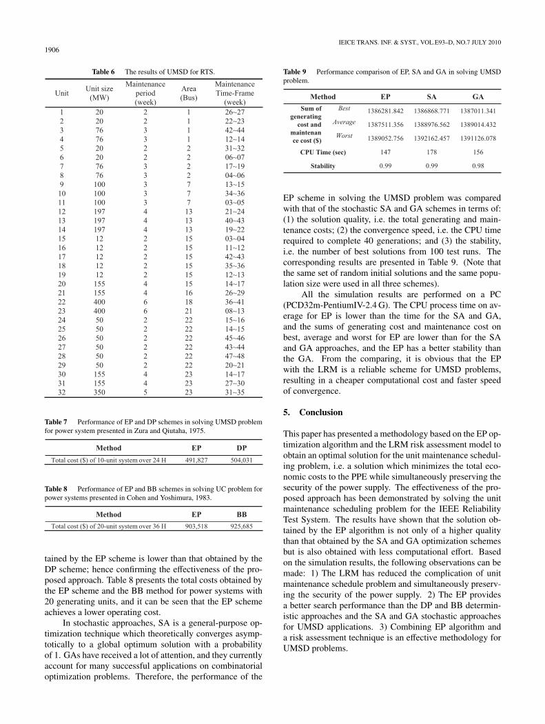
Table 9 Performance comparison of EP, SA and GA in solving UMSDproblem.

EP scheme in solving the UMSD problem was comparedwith that of the stochastic SA and GA schemes in terms of:(1) the solution quality, i.e. the total generating and main-tenance costs; (2) the convergence speed, i.e. the CPU timerequired to complete 40 generations; and (3) the stability,i.e. the number of best solutions from 100 test runs. Thecorresponding results are presented in Table 9. (Note thatthe same set of random initial solutions and the same popu-lation size were used in all three schemes).

All the simulation results are performed on a PC(PCD32m-PentiumIV-2.4 G). The CPU process time on av-erage for EP is lower than the time for the SA and GA,and the sums of generating cost and maintenance cost onbest, average and worst for EP are lower than for the SAand GA approaches, and the EP has a better stability thanthe GA. From the comparing, it is obvious that the EPwith the LRM is a reliable scheme for UMSD problems,resulting in a cheaper computational cost and faster speedof convergence.

5. Conclusion

This paper has presented a methodology based on the EP op-timization algorithm and the LRM risk assessment model toobtain an optimal solution for the unit maintenance schedul-ing problem, i.e. a solution which minimizes the total eco-nomic costs to the PPE while simultaneously preserving thesecurity of the power supply. The effectiveness of the pro-posed approach has been demonstrated by solving the unitmaintenance scheduling problem for the IEEE ReliabilityTest System. The results have shown that the solution ob-tained by the EP algorithm is not only of a higher qualitythan that obtained by the SA and GA optimization schemesbut is also obtained with less computational effort. Basedon the simulation results, the following observations can bemade: 1) The LRM has reduced the complication of unitmaintenance schedule problem and simultaneously preserv-ing the security of the power supply. 2) The EP providesa better search performance than the DP and BB determin-istic approaches and the SA and GA stochastic approachesfor UMSD applications. 3) Combining EP algorithm anda risk assessment technique is an effective methodology forUMSD problems.


References

[1] J. Schlabbach and K.H. Rofalski, Power System Engineering: Plan-ning, Design, and Operation of Power Systems and Equipment, JohnWiley & Sons, 2008.

[2] J. Zhu, Optimization of Power System Operation, John Wiley &Sons, 2009.

[3] C.E. Lin, C.J. Lin, C.C. Liang, and S.Y. Lee, “An expert systemfor generator maintenance scheduling using operation index,” IEEETrans. Power Appar. Syst., vol.7, no.3, pp.1141–1148, 1992.

[4] L.L. Garver, “Effective load carrying capability of generating units,”IEEE Trans. Power Appar. Syst., vol.PAS-85, no.8, pp.910–919,1966.

[5] L.L. Garver, “Adjusting maintenance schedules to levelized risk,”IEEE Trans. Power Appar. Syst., vol.PAS-91, no.5, pp.2057–2063,1972.

[6] K.W. Edwin and F. Curtius, “New maintenance scheduling methodwith production cost minimization via integer linear programming,”Int. J. Electrical Power and Energy Systems, vol.12, no.1, pp.165–170, 1990.

[7] H.H. Zura and V.H. Qiutaha, “Generation maintenance schedulingvia successive approximation dynamic programming,” IEEE Trans.Power Appar. Syst., vol.PAS-94, no.5, pp.665–671, 1975.

[8] A.I. Cohen and M. Yoshimura, “A branch-and-bound algorithm forunit commitment,” IEEE Trans. Power Appar. Syst., vol.PAS-102,no.2, pp.444–451, 1983.

[9] H. Sasaki, M. Watabable, J. Kubokawa, N. Yorino, and R.Yokoyama, “Maintenance scheduling years by artificial neural net-works,” Proc. ANNPS’93, Yokohama, Japan, 1993.

[10] T. Satoh and K. Nara, “Maintenance scheduling by using simu-lated annealing method,” IEEE Trans. Power Syst., vol.6, no.2,pp.850–856, 1991.

[11] R.C. Leou, “A new method for unit maintenance scheduling basedon genetic algorithm,” IEEE Power Engineering Society GeneralMeeting, vol.1, pp.246–251, 2003.

[12] K. Suresh and N. Kumarappan, “Combined genetic algorithm andsimulated annealing for preventive unit maintenance scheduling inpower system,” IEEE Power Engineering Society General Meeting,vol.1, pp.18–22, 2006.

[13] K. Hyunchul and H. Yasuhiro, “An algorithm for thermal unit main-tenance scheduling through combined use of GA and TS,” IEEE291-5 PWRS Winter Meeting, 1996.

[14] D.B. Fogel, System Identification through simulated evolution: Amachine learning approach to modeling, Ginn Press, 1991.

[15] D.B. Fogel, Evolutionary computation: Toward a New Philosophyof Machine Intelligence, IEEE Press, 1995.

[16] T. Back, Evolutionary Algorithms in Theory and Practice, OxfordUniv. Press, 1996.

[17] W.M. Lin, C.D. Yang, and M.T. Tsay, “Distribution system planningwith evolutionary programming and a reliability cost model,” IEEProc. — Generation, Transmission, and Distribution, vol.147, no.6,pp.336–341, 2000.

[18] H. Chen and X. Wang, “Cooperative co-evolutionary algorithmfor unit commitment,” IEEE Trans. Power Syst., vol.17, no.1,pp.128–133, 2002.

[19] C.S. Chang, “A real-time decision support system for voltage col-lapse avoidance in power supply networks,” IEICE Trans. Inf. &Syst., vol.E91-D, no.6, pp.1740–1747, June 2008.

[20] E.J. Henley and H. Kumamoto, Probabilistic Risk Assessment, IEEEPress, 1992.

[21] S. Stoft, Power System Economics: Designing Markets for Electric-ity, IEEE Press, 2002.

[22] W. Li, Risk Assessment of Power Systems: Models, Methods, andApplications, IEEE Press, 2005.

[23] Z.D. Bai, H.X. Liu, and W.K. Wong, “On the Markowitz mean-variance analysis of self-financing portfolios,” Risk and Decision

Analysis, vol.1, no.1, pp.35–42, 2009.[24] M. Choudhry, An Introduction to Value-at-Risk, John Wiley & Sons,

2006.[25] C. Alexander, Value-at-Risk Models, John Wiley & Sons, 2009.[26] P. Jorion, Value at Risk: The New Benchmark for Managing Finan-

cial Risk, McGraw-Hill, New York, 2006.[27] C.S. Chang, “The VaR applications for the unit maintenance

scheduling,” J. Management & Systems, vol.12, no.1, pp.75–92, Jan.2005.

[28] C. Grigg, “The IEEE reliability test system: 1996,” Paper 96 WM326-9 PWRS, IEEE Winter Power Meeting, 1996.

Appendix

Lemma A: Computation of risk characteristic coeffi-cient (m)

The current risk assessment scheme applies the approachproposed by Garver of GE (USA), i.e. an exponential func-tion is used to approximate the values of the VaR and therisk characteristic coefficient (m), as shown in Fig. A· 1.

In Fig. A· 1, the capacity size of the unit is first paintedon the semi-logarithmic coordinate axis. Points P and Q arethen connected to form a straight line (i.e. an exponentialfunction) with which to partially approximate V(X), V(X)is the VaR of a unit’s maintenance with reserve capacity X.The correlation between V(X) and the risk characteristic co-efficient m is expressed by

V(X) = α ∗ e−Xm , (A· 1)

where X is the reserve capacity of power system (in MW),and α is a constant (0.1 ∼ 1). The risk characteristic coeffi-cient (m) indicates the change in the forced outage capacitycaused by a change of e in the risk of the generating unit.In Fig. A· 1, the values of the VaR at points P and Q aregiven by

V(XP) = α ∗ e−XPm , (A· 2)

V(XQ) = α ∗ e−XQm , (A· 3)

Dividing Eq. (A· 2) by Eq. (A· 3) gives

V(XP)V(XQ)

= α ∗ eXQ−XP

m .

The risk characteristic coefficient, m, is therefore given by

Fig. A· 1 Use of exponential function to find approximate values of VaR.


m =XQ − XP

ln[V(XP)/V(XQ)]. (A· 4)

Lemma B: Computation of effective load carrying capac-ity (Ce) and equivalent load (Le)

(1) Computation of effective load carrying capacity (Ce)The combined impact on the VaR of a new unit joining

the generating operation and random outage events, respec-tively, can be expressed as

V(X) = p ∗ V(X + Y) + q ∗ V(X + Y −C). (A· 5)

where X: reserve capacity of power system;C: rated capacity of power system;Y: reserve capacity of affiliation for maintaining

a regular VaR when adding a unit;p: availability rate;q: forced outage rate (FOR), p + q = 1.

Substituting Eq. (A· 5) into Eq. (A· 1) gives

α ∗ e−(X+Y)

m ∗ p + α ∗ e−(X+Y−C)

m ∗ q = α ∗ e−Xm ,

e−(X+Y)

m ∗ p + e−(X+Y−C)

m ∗ q = e−Xm ,

e−(X+Y)

m ∗[p + q ∗ e

Cm

]= e−

Xm ,

e−Ym ∗[p + q ∗ e

Cm

]= 1,[

p + q ∗ eCm

]= e

Ym ,

Ym= ln[p + q ∗ e

Cm

],

Y = m ∗ ln[p + q ∗ e

Cm

].

Finally, the effective load carrying capacity is given by

Ce = C − Y = C − m ∗ ln[p + q ∗ e

Cm

]. (A· 6)

(2) Computation of equivalent load (Le)Taking account of the impact on the VaR of changes

in the daily load (i.e. the impact of the equivalent load), theVaR can be expressed as

Vi(X) = P(Ct − Le) ∗ Tp =

Tp∑j=1

V(Ct − Lj), (A· 7)

where Tp: total number of days in timeframe;Ct = C: rated capacity of power system;Le: equivalent load;Lj: maximum load on day j of timeframe.

Substituting Eq. (A· 7) into Eq. (A· 1) gives

Tp ∗ α ∗ e−(Ct−Le)

m =

Tp∑j=1

α ∗ e−(Ct−L j)

m .

Then, it can be shown that

Tp ∗ e−Ctm ∗ e

Lem = e

−Ctm ∗

Tp∑j=1

eL jm ,

Tp ∗ eLem =

Tp∑j=1

eL jm ,

eLem =

{ Tp∑j=1

eL jm/Tp

},

Le

m=

{ Tp∑j=1

eL jm/Tp

},

Finally, the equivalent load is given by:

Le = m ln

{ Tp∑j=1

eL jm/Tp

}(A· 8)

Chen-Sung Chang is an Associate Pro-fessor of Information Management at Nan-KaiUniversity of Technology. He received his Ph.D.in Electrical Engineering from National TaiwanUniversity in 1999. From 1988 to 2002, He waswith the Chunghwa Telecom. Co., Ltd. for Dept.of Information Management. His research in-terests include the applications of artificial in-telligence, soft computing and value-at-risk inpower systems.

Documents

Approach to the Unit Maintenance Scheduling Decision Using