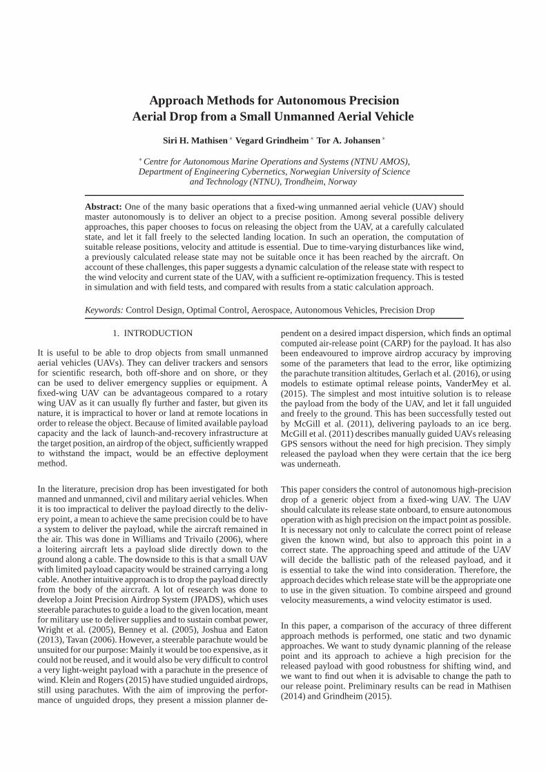
Approach Methods for Autonomous PrecisionAerial Drop from a Small Unmanned Aerial Vehicle

Siri H. Mathisen ∗ Vegard Grindheim ∗ Tor A. Johansen∗

∗ Centre for Autonomous Marine Operations and Systems (NTNU AMOS),Department of Engineering Cybernetics, Norwegian University of Science

and Technology (NTNU), Trondheim, Norway

Abstract: One of the many basic operations that a fixed-wing unmanned aerial vehicle (UAV) shouldmaster autonomously is to deliver an object to a precise position. Among several possible deliveryapproaches, this paper chooses to focus on releasing the object from the UAV, at a carefully calculatedstate, and let it fall freely to the selected landing location. In such an operation, the computation ofsuitable release positions, velocity and attitude is essential. Due to time-varying disturbances like wind,a previously calculated release state may not be suitable once it has been reached by the aircraft. Onaccount of these challenges, this paper suggests a dynamic calculation of the release state with respect tothe wind velocity and current state of the UAV, with a sufficient re-optimization frequency. This is testedin simulation and with field tests, and compared with resultsfrom a static calculation approach.

Keywords: Control Design, Optimal Control, Aerospace, Autonomous Vehicles, Precision Drop

1. INTRODUCTION

It is useful to be able to drop objects from small unmannedaerial vehicles (UAVs). They can deliver trackers and sensorsfor scientific research, both off-shore and on shore, or theycan be used to deliver emergency supplies or equipment. Afixed-wing UAV can be advantageous compared to a rotarywing UAV as it can usually fly further and faster, but given itsnature, it is impractical to hover or land at remote locations inorder to release the object. Because of limited available payloadcapacity and the lack of launch-and-recovery infrastructure atthe target position, an airdrop of the object, sufficiently wrappedto withstand the impact, would be an effective deploymentmethod.

In the literature, precision drop has been investigated forbothmanned and unmanned, civil and military aerial vehicles. Whenit is too impractical to deliver the payload directly to the deliv-ery point, a mean to achieve the same precision could be to havea system to deliver the payload, while the aircraft remainedinthe air. This was done in Williams and Trivailo (2006), wherea loitering aircraft lets a payload slide directly down to theground along a cable. The downside to this is that a small UAVwith limited payload capacity would be strained carrying a longcable. Another intuitive approach is to drop the payload directlyfrom the body of the aircraft. A lot of research was done todevelop a Joint Precision Airdrop System (JPADS), which usessteerable parachutes to guide a load to the given location, meantfor military use to deliver supplies and to sustain combat power,Wright et al. (2005), Benney et al. (2005), Joshua and Eaton(2013), Tavan (2006). However, a steerable parachute wouldbeunsuited for our purpose: Mainly it would be too expensive, as itcould not be reused, and it would also be very difficult to controla very light-weight payload with a parachute in the presenceofwind. Klein and Rogers (2015) have studied unguided airdrops,still using parachutes. With the aim of improving the perfor-mance of unguided drops, they present a mission planner de-

pendent on a desired impact dispersion, which finds an optimalcomputed air-release point (CARP) for the payload. It has alsobeen endeavoured to improve airdrop accuracy by improvingsome of the parameters that lead to the error, like optimizingthe parachute transition altitudes, Gerlach et al. (2016),or usingmodels to estimate optimal release points, VanderMey et al.(2015). The simplest and most intuitive solution is to releasethe payload from the body of the UAV, and let it fall unguidedand freely to the ground. This has been successfully tested outby McGill et al. (2011), delivering payloads to an ice berg.McGill et al. (2011) describes manually guided UAVs releasingGPS sensors without the need for high precision. They simplyreleased the payload when they were certain that the ice bergwas underneath.

This paper considers the control of autonomous high-precisiondrop of a generic object from a fixed-wing UAV. The UAVshould calculate its release state onboard, to ensure autonomousoperation with as high precision on the impact point as possible.It is necessary not only to calculate the correct point of releasegiven the known wind, but also to approach this point in acorrect state. The approaching speed and attitude of the UAVwill decide the ballistic path of the released payload, and itis essential to take the wind into consideration. Therefore, theapproach decides which release state will be the appropriate oneto use in the given situation. To combine airspeed and groundvelocity measurements, a wind velocity estimator is used.

In this paper, a comparison of the accuracy of three differentapproach methods is performed, one static and two dynamicapproaches. We want to study dynamic planning of the releasepoint and its approach to achieve a high precision for thereleased payload with good robustness for shifting wind, andwe want to find out when it is advisable to change the path toour release point. Preliminary results can be read in Mathisen(2014) and Grindheim (2015).

2. COMPUTED AIR-RELEASE POINT

Given the target location, a set of feasible release points canbe calculated, depending on incoming velocity, wind velocityand height over target. The choice of release point then decideshow to approach that position. Given the drag force equationFD = 1

2CDAρV 2a (Beard and McLain, 2012), whereCD is the

drag coefficient,ρ is the density of the fluid (air), A is theprojected area of the body relative to its movement andVa isthe speed of the body relative to the fluid. Newton’s 2nd law,assuming only drag force and gravity acting on the falling body,is:

m

[

vxvyvz

]

=−m

[

00g

]

+

[

FDxFDyFDz

]

, (1)

wherem is the mass of the body,g is the gravitational accelera-tion constant and the decomposed drag forces are:

FDx =−12

CDAρV2a

ur

Va,

FDy =−12

CDAρV2a

vr

Va, (2)

FDy =−12

CDAρV2a

wr

Va,

where the drag force is transformed from the wind frame to thebody frame of the object. The ballistic equations are given by:

x =

vxvyvz

−1

2mCDAρV 2

aur

Va

−1

2mCDAρV 2

avr

Va

−g−1

2mCDAρV 2

awr

Va

(3)

where the statesx = [x y z vx vy vz]⊤ is a vector of North-

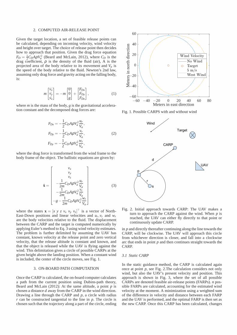
East-Down positions and linear velocities andur,vr and wrare the body velocities relative to the fluid. The displacementbetween the CARP and the target is computed numerically byapplying Euler’s method to Eq. 3 using wind velocity estimates.The problem is further delimited by assuming the UAV hasconstant, known velocity at the release point and zero verticalvelocity, that the release altitude is constant and known, andthat the object is released while the UAV is flying against thewind. This delimitation gives a circle of possible CARPs at thegiven height above the landing position. When a constant windis included, the center of the circle moves, see Fig. 1.

3. ON-BOARD PATH COMPUTATION

Once the CARP is calculated, the on-board computer calculatesa path from the current position using Dubins-path theory,Beard and McLain (2012): At the same altitude, a pointp ischosen a distanced away from the CARP in the wind direction.Drawing a line through the CARP andp, a circle with radiusr can be constructed tangential to the line inp. The circle ischosen such that the trajectory along a part of the circle, ending

Meters in east direction

Me

ters

inn

ort

hd

irect

ion

−60 −40 −20 0 20 40 60 80−60

−40

−20

0

20

40

60

Fig. 1. Possible CARPS with and without wind

Fig. 2. Initial approach towards CARP: The UAV makes aturn to approach the CARP against the wind. Whenp isreached, the UAV can either fly directly to that point orcontinuously update CARP.

in p and directly thereafter continuing along the line towards theCARP, will be clockwise. The UAV will approach this circlefrom whichever direction is closer, and fall into a clockwisearc that ends in pointp and then continues straight towards theCARP.

3.1 Static CARP

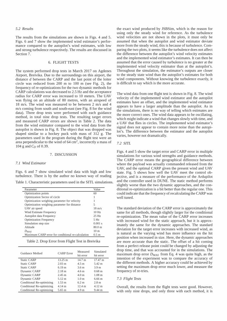
In the static guidance method, the CARP is calculated againonce at pointp, see Fig. 2.The calculation considers not onlywind, but also the UAV’s present velocity and position. Thisapproach is shown in Fig. 3, where the set of all possibleCARPs are denoted feasible air-release points (FARPs).n pos-sible FARPs are calculated, accounting for the estimated windvelocity at the moment. A minimization using a weighted sumof the difference in velocity and distance between each FARPand the UAV is performed, and the optimal FARP is then set asthe new CARP. Once this CARP has been calculated, changes

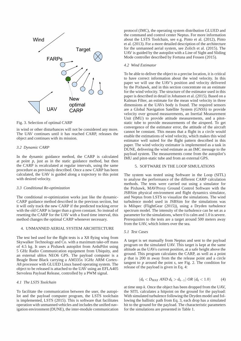
Fig. 3. Selection of optimal CARP

in wind or other disturbances will not be considered any more.The UAV continues until it has reached CARP, releases theobject and continues with its mission.

3.2 Dynamic CARP

In the dynamic guidance method, the CARP is calculatedat point p, just as in the static guidance method, but thenthe CARP is recalculated at regular intervals, using the sameprocedure as previously described. Once a new CARP has beencalculated, the UAV is guided along a trajectory to this pointwith desired velocity.

3.3 Conditional Re-optimization

The conditional re-optimization works just like the dynamic-CARP guidance method described in the previous section, butit will only track the new CARP if the predicted tracking errorwith the old CARP is larger than a given constant. So instead ofresetting the CARP for the UAV with a fixed time interval, thismethod changes the optimal CARP whenever necessary.

4. UNMANNED AERIAL SYSTEM ARCHITECTURE

The test bed used for the flight tests is a X8 flying wing fromSkywalker Technology and Co. with a maximum take-off massof 4.5 kg. It uses a Pixhawk autopilot from ArduPilot using5 GHz Radio Communication equipment from Ubiquity, andan external ublox NEO6 GPS. The payload computer is aBeagle Bone Black carrying a AM335x 1GHz ARM Cortex-A8 processor with GLUED Linux based operating system. Theobject to be released is attached to the UAV using an EFLA405Servoless Payload Release, controlled by a PWM signal.

4.1 The LSTS Toolchain

To facilitate the communication between the user, the autopi-lot and the payload computer program, the LSTS toolchainis implemented, LSTS (2015). This is software that facilitatesoperation with unmanned vehicles and includes the unified nav-igation environment (DUNE), the inter-module communication

protocol (IMC), the operating system distribution GLUED andthe command and control center Neptus. For more informationabout the LSTS Toolchain, see e.g. Pinto et al. (2012), Pintoet al. (2013). For a more detailed description of the architecturefor the unmanned aerial system, see Zolich et al. (2015). TheUAV is guided by the autopilot with a Line of Sight and SlidingMode controller described by Fortuna and Fossen (2015).

4.2 Wind Estimator

To be able to deliver the object to a precise location, it is criticalto have correct information about the wind velocity. In thispaper we will use the UAV’s position and velocity deliveredby the Pixhawk, and in this section concentrate on an estimatefor the wind velocity. The structure of the estimator used inthispaper is described in detail in Johansen et al. (2015). Basedon aKalman Filter, an estimate for the mean wind velocity in threedimensions at the UAVs body is found. The required sensorsare a Global Navigation Satellite System (GNSS) to providevelocity over ground measurements, an Inertial MeasurementUnit (IMU) to provide attitude measurements, and a pitot-static tube to provide measurements of the airspeed. To getconvergence of the estimator error, the attitude of the aircraftcannot be constant. This means that a flight in a circle wouldenable the estimations of wind velocity, which makes this windestimator well suited for the flight pattern described in thispaper. The wind velocity estimator is implemented as a task inDUNE, delivering the wind estimate as an IMC message to thepayload system. The measurements come from the autopilot’sIMU and pitot-static tube and from an external GPS.

5. SOFTWARE IN THE LOOP SIMULATIONS

The system was tested using Software in the Loop (SITL)to analyse the performance of the different CARP calculationmethods. The tests were carried out using a simulator forthe Pixhawk, MAVProxy Ground Control Software with theJSBSim physical environment and flight dynamics simulator,and Neptus from LSTS to visualize the simulations. The windturbulence model used in JSBSim for the simulations wasis Milspec (FlightGear (2015)), using a Dryden turbulencespectrum model. The intensity of the turbulence can be set asaparameter for the simulations, where 0 is calm and 1.0 is severe.Prerequisites to the tests are a target around 500 meters awayfrom the UAV, which loiters over the sea.

5.1 Test Cases

A target is set manually from Neptus and sent to the payloadprogram on the simulated UAV. This target is kept at the samealtitude as the UAVs current position, at a safe height abovetheground. This program calculates the CARP, as well as a pointp that is 200 m away from the the release point and a circletangent top around the points, see Fig. 2. The condition forrelease of the payload is given in Eq. 4:

(dk < DMAX AND dk > dk−1) OR (dk < 1.0) (4)

at time stepk. Once the object has been dropped from the UAV,the SITL calculates a hitpoint on the ground for the payload:With simulated turbulence following the Dryden model and fol-lowing the ballistic path from Eq. 3, each drop has a simulatedhit to the ground for the payload. The characteristic parametersfor the simulations are presented in Table 1.

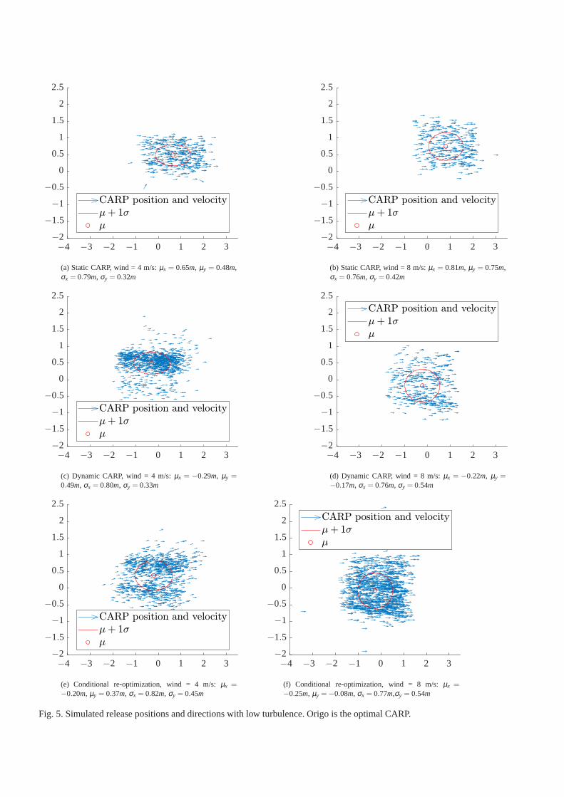
5.2 Results

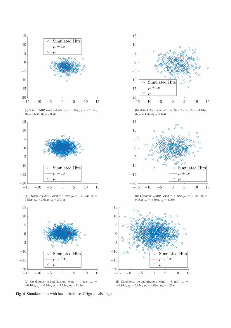
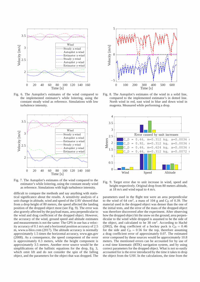
The results from the simulations are shown in Figs. 4 and 5.Figs. 6 and 7 show the implemented wind estimator’s perfor-mance compared to the autopilot’s wind estimates, with lowand strong turbulence respectively. The results are discussed inSection 7.

6. FLIGHT TESTS

The system performed drop tests in March 2017 on AgdenesAirport, Breivika. Due to the surroundings on this airport,thedistanced between the CARP and the last point of the loitercircle was reduced from 200 m to 100 m (see Fig. 2), thefrequency of re-optimizations for the two dynamic methods forCARP calculations was decreased to 2.5 Hz and the acceptanceradius for CARP error was increased to 10 meters. The UAVwas flying on an altitude of 80 metres, with an airspeed of18 m/s. The wind was measured to be between 2 m/s and 4m/s coming from south and south-east (see Fig. 8 for the winddata). Three drop tests were performed with each guidancemethod, in total nine drop tests. The resulting target errorsand measured CARP errors are shown in Table 2. The datafrom the wind estimator compared to the wind data from theautopilot is shown in Fig. 8. The object that was dropped wasshaped similar to a hockey puck with mass of 312 g. Theparameters used in the program during the flight test were anarea perpendicular to the wind of 64 cm2, incorrectly a mass of104 g andCD of 0.39.

7. DISCUSSION

7.1 Wind Estimator

Figs. 6 and 7 show simulated wind data with high and lowturbulence. There is by the author no known way of reading

Table 1. Characteristic parameters used in the SITL simulations.

Parameter ValueOptimization points 60Optimization Sector of circle 1Optimization weighing parameter for velocity 1Optimization weighing parameter for distance 5UAV air speed 18 m/sWind Estimate Frequency 10 HzAutopilot data Frequency 25 HzOptimization Frequency 5 HzSimulation step size 0.001 sAltitude 80.0 mDMAX 10 mMaximum CARP error for conditional re-calculation 0.5 m

Table 2. Drop Error from Flight Test in Breivika

Guidance Method CARP Error Measuredhit error

Simulatedhit error

Static CARP 13.25 m 14.7 m 17.47 mStatic CARP 2.03 m 4.5 m 5.42 mStatic CARP 6.19 m 3.6 m 3.9 mDynamic CARP 2.18 m 4.6 m 0.68 mDynamic CARP 2.45 m 4.0 m 1.08 mDynamic CARP 5.12 m 1.0 m 6.66 mConditional Re-optimizing 1.53 m 6.2 m 2.8 mConditional Re-optimizing 4.14 m 12.4 m 4.12 mConditional Re-optimizing 5.65 m 4.9 m 9.44 m

the exact wind produced by JSBSim, which is the reason forusing only the steady wind for reference. As the turbulencewind velocities are not shown in the plots, it must only beassumed that when the autopilot and wind estimator deviatemore from the steady wind, this is because of turbulence. Com-paring the two plots, it seems like the turbulence does not affectthe difference between the autopilot’s wind velocity estimatesand the implemented wind estimator’s estimates. It can thenbeassumed that the error caused by turbulence is no greater at theimplemented wind velocity estimator than at the autopilot’s.Throughout the simulation, the estimator’s outputs are closerto the steady state wind than the autopilot’s estimates for bothwind components. Without knowing the turbulence exactly, itis difficult to say which is the more accurate.

The wind data from one flight test is shown in Fig. 8. The windvelocity of the implemented wind estimator and the autopilotestimates have an offset, and the implemented wind estimatorappears to have a larger amplitude than the autopilot. As inthe simulations, there is no way of telling which estimates arethe more correct ones. The wind data appears to be oscillating,which might indicate a wind that changes slowly with time, anda UAV that flies in circles. The implemented wind estimator’ssignal does not appear to contain more noise than the autopi-lot’s. The difference between the estimator and the autopilotvaries, however not dramatically.

7.2 SITL

Figs. 4 and 5 show the target error and CARP error in multiplesimulations for various wind strengths and guidance methods.The CARP error means the geographical difference betweenwhere the payload was actually commanded released from theUAV, and the optimal CARP given the present wind and UAVstate. Fig. 5 shows how well the UAV meet the control ob-jective, and is a measure of the performance of the Ardupilotand the controller used in DUNE. The static method performsslightly worse than the two dynamic approaches, and the con-ditional re-optimization is a bit better than the regular one. Thiscould indicate that the frequency of recalculating the CARPwaswell tuned.

The standard deviation of the CARP error is approximately thesame for all methods, though slightly larger for the conditionalre-optimization. The mean value of the CARP error increaseswith increased wind for the static approach, but it is approx-imately the same for the dynamic approaches. The standarddeviation for the target error increases with increased wind, asis natural as the varying wind has more influence on the hitposition when increased in size. Here, the dynamic approachesare more accurate than the static. The offset of a hit comingfrom a perfect release point could be changed by adjusting thedrop time, and that was accounted for in the simulations. Themaximum drop errorDMAX from Eq. 4 was quite high, as theintention of the experiment was to compare the accuracy ofthe different methods. A higher accuracy could be achieved bysetting the maximum drop error much lower, and measure thefrequency of re-tries.

7.3 Flight Tests

Overall, the results from the flight tests were good. However,with only nine drops, and only three with each method, it is

−15 −10 −5 0 5 10 15−20

−15

−10

−5

0

5

10

15

(a) Static CARP, wind = 4 m/s:µx = 1.60m, µy =−2.51m,σx = 2.68m, σy = 2.05m

−15 −10 −5 0 5 10 15−20

−15

−10

−5

0

5

10

15

(b) Static CARP, wind = 8 m/s:µx = 2.21m, µy =−1.01m,σx = 4.39m, σy = 3.94m

−15 −10 −5 0 5 10 15−20

−15

−10

−5

0

5

10

15

(c) Dynamic CARP, wind = 4 m/s:µx = −0.11m, µy =0.51m, σx = 2.61m, σy = 2.01m

−15 −10 −5 0 5 10 15−20

−15

−10

−5

0

5

10

15

(d) Dynamic CARP, wind = 8 m/s:µx = 0.14m, µy =0.15m, σx = 4.50m, σy = 4.09m

−15 −10 −5 0 5 10 15−20

−15

−10

−5

0

5

10

15

(e) Conditional re-optimization, wind = 4 m/s:µx =−0.16m, µy = 0.36m, σx = 2.78m, σy = 2.12m

−15 −10 −5 0 5 10 15−20

−15

−10

−5

0

5

10

15

(f) Conditional re-optimization, wind = 8 m/s:µx =−0.14m, µy = 0.13m, σx = 4.66m, σy = 4.20m

Fig. 4. Simulated hits with low turbulence. Origo equals target.

−4 −3 −2 −1 0 1 2 3−2

−1.5

−1

−0.5

0

0.5

1

1.5

2

2.5

(a) Static CARP, wind = 4 m/s:µx = 0.65m, µy = 0.48m,σx = 0.79m, σy = 0.32m

−4 −3 −2 −1 0 1 2 3−2

−1.5

−1

−0.5

0

0.5

1

1.5

2

2.5

(b) Static CARP, wind = 8 m/s:µx = 0.81m, µy = 0.75m,σx = 0.76m, σy = 0.42m

−4 −3 −2 −1 0 1 2 3−2

−1.5

−1

−0.5

0

0.5

1

1.5

2

2.5

(c) Dynamic CARP, wind = 4 m/s:µx = −0.29m, µy =0.49m, σx = 0.80m, σy = 0.33m

−4 −3 −2 −1 0 1 2 3−2

−1.5

−1

−0.5

0

0.5

1

1.5

2

2.5

(d) Dynamic CARP, wind = 8 m/s:µx = −0.22m, µy =−0.17m, σx = 0.76m, σy = 0.54m

−4 −3 −2 −1 0 1 2 3−2

−1.5

−1

−0.5

0

0.5

1

1.5

2

2.5

(e) Conditional re-optimization, wind = 4 m/s:µx =−0.20m, µy = 0.37m, σx = 0.82m, σy = 0.45m

−4 −3 −2 −1 0 1 2 3−2

−1.5

−1

−0.5

0

0.5

1

1.5

2

2.5

(f) Conditional re-optimization, wind = 8 m/s:µx =−0.25m, µy =−0.08m, σx = 0.77m,σy = 0.54m

Fig. 5. Simulated release positions and directions with lowturbulence. Origo is the optimal CARP.

Time [s]

Ve

loci

ty[m

/s]

0 20 40 60 80 100 120 140 160

2

2.5

3

3.5

Fig. 6. The Autopilot’s estimates of the wind compared tothe implemented estimator’s while loitering, using theconstant steady wind as reference. Simulations with lowturbulence intensity.

Time [s]

Ve

loci

ty[m

/s]

0 20 40 60 80 100120 140 160

2

2.5

3

3.5

Fig. 7. The Autopilot’s estimates of the wind compared to theestimator’s while loitering, using the constant steady windas reference. Simulations with high turbulence intensity.

difficult to compare the methods and say anything with statis-tical significance about the results. A sensitivity analysis of aunit change in altitude, wind and speed of the UAV showed thatfrom a drop height of 80 meters, the speed affected the landingposition of the dropped object most (see Fig. 9). The error wasalso gravely affected by the payload mass, area perpendicular tothe wind and drag coefficient of the dropped object. However,the accuracy of the wind, ground speed and altitude estimatesand measurements is not the same: The GPS in use has a veloc-ity accuracy of 0.1 m/s and a horizontal position accuracy of2.5m, www.u-blox.com (2017). The altitude accuracy is normallyapproximately 1.5 times the horizontal accuracy, www.gps.gov(2008). As a consequence, the speed component of the erroris approximately 0.3 meters, while the height component isapproximately 3.5 meters. Another error source would be thesimplifications of the ballistic equations for the drop, Eq.3,which omit lift and do not consider the spin of the fallingobject, and the parameters for the object that was dropped. The

Time [s]

Ve

loci

ty[m

/s]

0 100 200 300 400 500 600−5

0

5

Fig. 8. The Autopilot’s estimates of the wind in a solid line,compared to the implemented estimator’s in dotted line.North wind in red, east wind in blue and down wind inmagenta. Measured while performing a drop.

C_D = 0.46, m=0.312 kg, a=0.0036 m^2C_D = 0.92, m=0.312 kg, a=0.0036 m^2C_D = 0.46, m=0.624 kg, a=0.0036 m^2C_D = 0.46, m=0.312 kg, a=0.0072 m^2

Me

ters

Wind Speed Altitude0

0.5

1

1.5

2

2.5

3

3.5

4

Fig. 9. Target error due to unit increase in wind, speed andheight respectively. Original drop from 80 meters altitude,at 18 m/s and wind equal to 4 m/s.

parameters used in the flight test were an area perpendicularto the wind of 64 cm2, a mass of 104 g andCD of 0.39. Thematerial used in the dropped object was denser than the one ofthe initial tests, and the error of the mass of the dropped objectwas therefore discovered after the experiment. After observinghow the dropped object hit the snow on the ground, area perpen-dicular to the wind while dropped is assumed to be the side ofthe object, and calculated to be 38 cm2. According to Hache(2002), the drag coefficient of a hockey puck isCD = 0.46for the side andCD = 0.56 for the top, therefore assuminga drag coefficient error of approximately 0.07. The estimatederror composed by these sources would be approximately 10.8meters. The mentioned errors can be accounted for by use ofa real time kinematic (RTK) navigation system, and by usingcorrect parameters for the dropped object. What is not so easilyaccounted for is the error introduced by the time it takes to dropthe object from the UAV. In the calculations, the time from the

signal is sent to the object is falling freely is set to 0.4 s. Thishas been tested in the lab, but not in the air, with a moving UAV.

ACKNOWLEDGEMENTS

This work is part of a project partly funded by the ResearchCouncil of Norway through the Centers of Excellence fund-ing scheme, project number 223254, NTNU Centre for Au-tonomous Marine Operations and Systems. This work couldnever have been carried out without the assistance given by thepilots and engineers at Norwegian University of Science andTechnology, and the authors are also grateful to Thor I. Fossenfor useful discussions on the topic.

REFERENCES

Beard, R.W. and McLain, T.W. (2012). Small unmannedaircraft: Theory and practice. Princeton University Press.

Benney, R., Barber, J., McGrath, J., McHugh, J., Noetscher,G., and Tavan, S. (2005). The new military applications ofprecision airdrop systems. InInfotech at Aerospace.

FlightGear (2015). JSBSim Atmosphere. URLwiki.flightgear.org JSBSim Atmosphere. .

Fortuna, J. and Fossen, T.I. (2015). Cascaded line-of-sight path-following and sliding mode controllers for fixed-wing uavs.In Proc. of the 2015 IEEE Multi-Conference on Systemsand Control. 2015 IEEE Multi-Conference on Systems andControl.

Gerlach, A.R., Manyam, S.G., and Doman, D.B. (2016). Pre-cision airdrop transition altitude optimization via the one-in-a-set traveling salesman problem. InAmerican ControlConference (ACC).

Grindheim, V. (2015).Accurate Drop of GPS Beacon Usingthe X8 Fixed-Wing UAV. Master’s thesis, Norwegian Univer-sity of Science and Technology, Department of EngineeringCybernetics.

Hache, A. (2002). The Physics of Hockey. Johns HopkinsUniversity Press.

Johansen, T.A., Cristofaro, A., Sorensen, K.L., Hansen, J.M.,and Fossen, T.I. (2015). On estimation of wind velocity,angle-of-attack and sideslip angle of small uavs using stan-dard sensors. InInternational Conference on UnmannedAircraft Systems.

Joshua, M. and Eaton, A.N. (2013). Point of impact: Deliveringmission essential supplies to the warfighter through the jointprecision airdrop system. InSystems Conference (SysCon).

Klein, B. and Rogers, J.D. (2015). A probabilistic approachto unguided airdrop. InAerodynamic Decelerator SystemsTechnology Conferences.

LSTS (2015). LSTS Toolchain. URLhttp://lsts.fe.up.pt/toolchain. .

Mathisen, S.H. (2014).High Precision Deployment of WirelessSensors from Unmanned Aerial Vehicles. Master’s thesis,Norwegian University of Science and Technology, Facultyof Information Technology, Mathematics and Electrical En-gineering, Department of Engineering Cybernetics.

McGill, P., Reisenbichler, K., Etchemendy, S., Dawe, T., andHobson, B. (2011). Aerial surveys and tagging of free-drifting icebergs using an unmanned aerial vehicle (uav).Deep Sea Research Part II: Topical Studies in Oceanogra-phy, 58.

Pinto, J., Calado, P., Braga, J., Dias, P., Martins, R., Marques,E., and Sousa, J. (2012). Implementation of a control archi-tecture for networked vehicle systems. In3rd IFAC Work-

shop on Navigation, Guidance and Control of UnderwaterVehicles.

Pinto, J., Dias, P.S., Martins, R., Fortuna, J., Marques, E., andSousa, J. (2013). The lsts toolchain for networked vehiclesystems. InOCEANS - Bergen, 2013 MTS/IEEE.

Tavan, S. (2006). Status and context of high altitude precisionaerial delivery systems. InAIAA Guidance, Navigation, andControl Conference and Exhibit Keystone.

VanderMey, J.T., Doman, D.B., and Gerlach, A.R. (2015). Re-lease point determination and dispersion reduction for ballis-tic airdrops. Journal of Guidance, Control, and Dynamics,38(11).

Williams, P. and Trivailo, P. (2006). Cable-supported slid-ing payload deployment from a circling fixed-wing aircraft.Journal of Aircraft, 43(5), 1567–1570.

Wright, R., Benney, R., and McHugh, J. (2005). Precisionairdrop system. In18th AIAA Aerodynamic DeceleratorSystems Technology Conference and Seminar.

www.gps.gov (2008). Global positioning system standardpositioning service performance standard. .

www.u-blox.com (2017). Neo-6 u-blox 6 GPS Modules DataSheet. .

Zolich, A.P., Johansen, T.A., Cisek, K.P., and Klausen, K.(2015). Unmanned aerial system architecture for maritimemissions. design and hardware description. InWorkshop onResearch, Education and Development of Unmanned AerialSystems (RED UAS).