Applying the Chi-Square Test to Improve the Performance of

Journal of Computers Vol. 29 No. 6, 2018, pp. 1-15

doi:10.3966/199115992018122906001

1

Applying the Chi-Square Test to Improve

the Performance of the Decision Tree for Classification

by Taking Baseball Database as an Example

Chia-En Li*, Ye-In Chang

Department of Computer Science and Engineering, National Sun Yat-sen University,

Kaohsiung 804, Taiwan

[email protected], [email protected]

Received 21 June 2017; Revised 19 September 2017; Accepted 1 December 2017

Abstract. The chi-square test is one of the statistical tests and is good to analyze whether

categorical variable A is the significant factor to categorical variable B. On the other hand, a

decision tree is one of useful models for data classification. To achieve the goal of efficient

knowledge discovery by a compact decision tree, in this paper, we propose a method by making

use of the result of the chi-square test to reduce the number of concerned attributes. We make

use of the P-value from the chi-square test to decide the significant factors as the preprocessing

step to prune insignificant factors before constructing the decision tree. In such a way, we can

avoid constructing the inaccurate decision tree. We use the public baseball database as an

example to illustrate our method. From our performance study, we observe that the way of

checking the most significant factor (i.e., the factor with the minimum P-value) first can reduce

the number of conditions (i.e., levels) to be decided. Therefore, the compact decision tree

constructed from our method can provide less storage cost, faster prediction time and higher

degree of accuracy for data classification than the decision tree concerning all original factors.

Keywords: chi-square test, classification, data mining, decision tree, significant factor

1 Introduction

In the real word, a large amount of data focusing on the same topic could have been collected as a topic-

related digital database. Therefore, knowledge discovery from such a topic-related digital database has

become an important research area in recent years. For this purpose, statistical tests and data mining

techniques have been largely studied, developed and applied for many fields [1-9].

The chi-square test is one of the statistical tests, and is designed to analyze whether a significant

relationship exists between two categorical variables. Furthermore, it is used in many fields including

medical studies [1-2], finance and market [3-4], education [5-6] and sports [7-9]. If the P-value from the

chi-square test between these two categorical variables is less than the given significant level which is

usually a very small number, there is a significant relationship between these two categorical variables.

The reason is that the computation of the chi-square test is to calculate the possibility of a null

assumption which is in contrast to our goal to conclude the strongly significant relationship between

these two categorical variables. Therefore, by using the chi-square test between the main-role attribute

and every concerned factor, we can conclude significant factors regaled to the main-role attribute.

Especially, in the field of medical studies, the significant factor is called the risk factor, since the factor is

usually for the disease [2].

On the other hand, classification is one of main topics of data mining. The goal of classification is to

predict the class of the new data after processing given data with the known class. One of well-known

models for classification is the decision tree model [10]. The decision tree is a direct graph (top-down)

* Corresponding Author

Applying the Chi-Square Test to Improve the Performance of the Decision Tree for Classification by Taking Baseball Database as an Example

2

with the internal node being the deciding attribute and the leaf node being the decided class [11]. The

decision tree has been widely applied to many areas, including medical diagnosis [12], risk analysis [13],

and sport [14]. We can use the decision tree model to classify unknown data and then calculate the

accuracy. Basically, the task of the decision tree algorithm is composed of two steps. First, we need to

create a decision tree by the given data (called training data) from the database. Second, we classify

future unknown cases (called testing data) by the rules in the model [15-16].

Therefore, both the chi-square test and the decision tree algorithm for analysis and classification are

good and well-known methods for knowledge discovery of digital data. However, there are few studies to

combine both methods to solve the same problem and analyze the relationship between these two

methods. To achieve the goal of efficient knowledge discovery by a compact decision tree, in this paper,

we propose a method by making use of the result of the chi-square test to reduce the number of

concerned attributes. We make use of the P-value from the chi-square test to decide the significant

factors as the preprocessing step to prune insignificant factors before constructing the decision tree. In

such a way, we can avoid constructing the inaccurate decision tree from unnecessary data. Because the

insignificant factors interfere with the decision tree for classification. We use the public baseball database

as an example with each of factors concerned in evaluating the performance of a batter as attribute A and

the AVG (batting average) as attribute B (i.e. the decided class) to illustrate our method. Moreover, we

use one of well-known decision tree construction algorithms, C4.5 [17-18]. Based on the same C4.5

algorithm for constructing the decision tree, we have compared the performance of the case that it uses

the preprocessing step and the case that it does not use the preprocessing step. From our performance

study, we observe that the most significant factor (i.e., the factor with the minimum P-value) is checked

first can reduce the number of conditions (i.e., levels) to be decided. This property also affects the

average number of conditions needed to be checked, the storage cost and the accuracy of prediction.

Therefore, the compact decision tree constructed from our method can provide less storage cost, faster

prediction time and higher degree of accuracy for data classification than the decision tree concerning all

original factors.

The rest of the paper is organized as follows. Section 2 describes the basic idea of the chi-square test

and the decision tree algorithm. Section 3 presents the proposed method. Section 4 gives the experiment

results and discussion of the relationship between the significant factors and the decision tree algorithm.

Finally, we give a conclusion in Section 5.

2 Background

In this section, we describe two well-known approaches for knowledge discovery. One is the statistical

test, chi-square test (X2), and the other one is the data mining algorithm for classification, the decision

tree algorithm.

2.1 The Chi-Square Test

The chi-square test is one of the statistical tests. In statistics, there are two types of attributes including

continuous numbers and categorical variables. Examples of continuous number are age and weight.

Moreover, examples of categorical variables are gender and location. If the attribute is a continuous

number, we have to convert the continuous number to a categorical variable. Afterwards, we can use the

number of categorical variables to calculate the P-value from the chi-square test. The chi-square test is

applied to determine whether there is a significant relationship between the two categorical variables

from database [19-21]. There are four steps in the chi-square test described as follows.

Step 1. State the null hypothesis (H0) and alternative hypothesis (Ha): The meaning of the null

hypothesis H0 and the meaning of hypothesis Ha between categorical variable A and variable B are as

follows:

H0: categorical variable A and categorical variable B are independent,

Ha: categorical variable A and categorical variable B are dependent.

Step 2. Determine the significant level: The significant level is used to decide whether to accept or

reject the null hypothesis. For the significant level, a value between 0 and 1 is used. However, one of the

values of the significant level is often chosen from 0.01, 0.05, or 0.10. Moreover, the chi-square test is

Journal of Computers Vol. 29, No. 6, 2018

3

used to determine whether there is a significant relationship between the two categorical variables. If the

P-value is less than the significant level, we reject the null hypothesis (H0) and accept alternative

hypothesis (Ha); otherwise, we accept the null hypothesis (H0).

Step 3. Analyze the database: In this step, there are four elements which have to be found. These

elements are the degree of freedom (DF), expected count (E), statistic test, and the P-value, separately.

Assume that the number of possible values of categorical variable A is r, and the number of possible

values of categorical variable B is c. First, the degree of freedom (DF) is defined as follows: DF = (r - 1)

× (c - 1). Second, the expected count (Er,c) is computed for each level of categorical variable A at each

level of categorical variable B. nr is the total number of observations at level r of categorical variable A.

Moreover, nc is the total number of observations at level c of categorical variable B. Furthermore, n is the

size of the data set. Er,c is the expected count for level r of categorical variable A and level c of

categorical variable B. The expected count (Er,c) is defined as follows: Er,c = (nr × nc) / n. Third, the

statistic test, chi-square test (X2), is defined as follows: X2 = ∑ [(Or,c – Er,c)2 / Er,c]. In this equation, Or,c is

the observed frequency for level r of categorical variable A and level c of categorical variable B. Finally,

we can use the chi-square distribution table to find the closet P-value associated with the degree of

freedom (DF) and the value of the chi-square (X2). The P-value means that the probability which the

deviation of the observation from that expected is due to chance alone.

Step 4. Explain the results in terms of the hypothesis: Referring to the chi-square distribution table,

we use the degree of freedom (DF) and the value of the chi-square test (X2) to find the closet P-value.

The chi-square distribution table is shown in Table 1. If the P-value is less than the significance level, we

reject the null hypothesis (H0) and accept the alternative hypothesis (Ha). Otherwise, we accept the null

hypothesis (H0) and reject the alternative hypothesis (Ha).

Table 1. The chi-square distribution table

Probability (P) DF

0.95 0.90 0.80 0.70 0.50 0.30 0.20 0.10 0.05 0.01 0.001

1 0.004 0.02 0.06 0.15 0.45 1.07 1.64 2.71 3.84 6.64 10.83

2 0.10 0.21 0.45 0.71 1.39 2.41 3.22 4.60 5.99 9.21 13.82

3 0.35 0.58 1.01 1.42 2.37 3.66 4.64 6.25 7.82 11.34 16.27

4 0.71 1.06 1.65 2.20 3.36 4.88 5.99 7.78 9.49 13.28 18.47

5 1.14 1.61 2.34 3.00 4.35 6.06 7.29 9.24 11.07 15.09 20.52

2.2 The Decision Tree

One of the well-established approaches for predictive models (i.e., classification) in data mining is the

decision tree [22]. ID3 algorithm and C4.5 algorithm are the well-known algorithms for building the

decision tree [17-18, 23-24]. In the ID3 algorithm [23], it evaluates the best splitting criterion of the

attributes during the tree building phase. It uses attribute A to partition the given data horizontally. The

ID3 algorithm selects the splitting attribute that minimizes the information entropy of the partition, when

selecting the best partition. The entropy function shows how disorderly a set is. The information gain

G(Ai) means the gain that the original set S obtains after split by attribute Ai. When a set of objects S is

encountered, the information gain of each available attribute is calculated and the one whose information

gain is the maximal is chosen as the classifying attribute for set S. It performs the calculation until each

subset is either pure or sufficiently small. The C4.5 algorithm is proposed in [17-18], and improves the

deficiency of information gain adopted in ID3. The criterion of information gain for the attribute

selection adopted in ID3 has a serious deficiency: it has a strong bias in favor of the attributes with many

values. In other words, if attribute A has more possible values in training data than attribute B, G(A)

tends to be larger than G(B).

3 The Proposed Method

In this section, we first describe the property of the baseball database which we use in our study. Next,

we describe our proposed method. Finally, we use the public baseball database as an example to illustrate

our method.


4

3.1 The Baseball Database

The World Baseball Softball Confederation (WBSC) has 208 National Federation Members in 141

countries and territories across Asia, Africa, Americas, Europe and Oceania [25]. In this sport, the

responsibility for baseball players is to score more runs than the other team when they are batters. In the

real world, a large amount of baseball batting data has been collected as digital database.

As stated in [26], each team plays 120 games in a year since 2009. There are 659 baseball players who

have at bats identified through Chinese Professional Baseball League (CPBL) team website from 2009 to

2015 [27]. The order of the original data is in the descending order of the number of games. In this paper,

we focus on the data of 132 baseball players whose at bats (AB) are greater than or equal to 372, and the

order is not important in this study. (Note that at bats is equal to the number of games multiplied 3.1

according to the rule which is recorded on the rule 9.22(a) of the official baseball rules 2017 edition on

the Major League Baseball (MLB) website [28] and the Chinese Professional Baseball League (CPBL),

2017 [29]. Therefore, we have 120 × 3.1 = 372.) They are reviewed for the thirteen factors including

games (G), plate appearances (PA), at bats (AB), run batted in (RBI), runs (R), hits (H), one-base hit (1B),

two-base hit (2B), three-base hit (3B), home run (HR), total bases (TB), strike outs (SO), and stolen bases

(SB). Furthermore, batting average (AVG) is reviewed in this study. Batting average (AVG) has been

often used to evaluate a batter whose batting performance is excellent or not. In general, the cut-off value

of batting average (AVG) is defined as 0.300 [30]. (Note that the value is discussable.) When the batting

data is greater than or equal to the cut-off value, it means that the batter has excellent betting performance.

3.2 Our Proposed Method

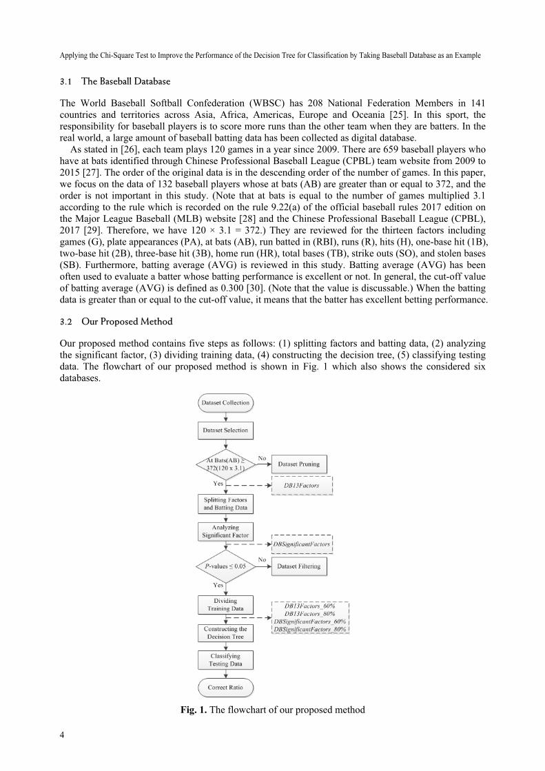
Our proposed method contains five steps as follows: (1) splitting factors and batting data, (2) analyzing

the significant factor, (3) dividing training data, (4) constructing the decision tree, (5) classifying testing

data. The flowchart of our proposed method is shown in Fig. 1 which also shows the considered six

databases.

Fig. 1. The flowchart of our proposed method


5

In Step 1, we split factors and batting data such that only categorical symbols are concerned for the

following steps. All of the thirteen factors are split based on the statistical mean, respectively.

Furthermore, the cut-off value of batting average (AVG) is defined as 0.300. If the possible value of the

attribute is a continuous number, we have to convert such a continuous number into a categorical symbol.

For example, the statistical mean of stolen bases (SB) is 10. We categorize stolen bases (SB) <10 as a

symbol 1 and stolen bases (SB) ≥10 as the other symbol 2. Moreover, we symbolize the new added

attribute, batting average (AVG). If it is greater than or equal to 0.300, we symbolize it by class A;

otherwise, we symbolize it by class B.

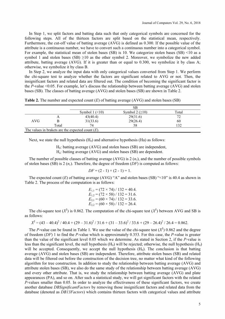
In Step 2, we analyze the input data with only categorical values converted from Step 1. We perform

the chi-square test to analyze whether the factors are significant related to AVG or not. Then, the

insignificant factors and related data are filtered out. The condition of becoming the significant factor is

the P-value <0.05. For example, let’s discuss the relationship between batting average (AVG) and stolen

bases (SB). The classes of batting average (AVG) and stolen bases (SB) are shown in Table 2.

Table 2. The number and expected count (E) of batting average (AVG) and stolen bases (SB)

SB

Symbol 1 (<10) Symbol 2 (≥10) Total

A 43(40.4) 29(31.6) 72

B 31(33.6) 29(26.4) 60 AVG

Total 74 58 132

The values in brakets are the expected count (E).

Next, we state the null hypothesis (H0) and alternative hypothesis (Ha) as follows:

H0: batting average (AVG) and stolen bases (SB) are independent,

Ha: batting average (AVG) and stolen bases (SB) are dependent.

The number of possible classes of batting average (AVG) is 2 (nr), and the number of possible symbols

of stolen bases (SB) is 2 (nc). Therefore, the degree of freedom (DF) is computed as follows:

DF = (2 - 1) × (2 - 1) = 1.

The expected count (E) of batting average (AVG) “A” and stolen bases (SB) “<10” is 40.4 as shown in

Table 2. The process of the computation is as follows:

E1,1 = (72 × 74) / 132 = 40.4.

E1,2 = (72 × 58) / 132 = 31.6.

E2,1 = (60 × 74) / 132 = 33.6.

E2,2 = (60 × 58) / 132 = 26.4.

The chi-square test (X2) is 0.862. The computation of the chi-square test (X2) between AVG and SB is

as follows:

X2 = (43 – 40.4)2 / 40.4 + (29 – 31.6)2 / 31.6 + (31 – 33.6)2 / 33.6 + (29 – 26.4)2 / 26.4 = 0.862.

The P-value can be found in Table 1. We use the value of the chi-square test (X2) 0.862 and the degree

of freedom (DF) 1 to find the P-value which is approximately 0.353. For this case, the P-value is greater

than the value of the significant level 0.05 which we determine. As stated in Section 2, if the P-value is

less than the significant level, the null hypothesis (H0) will be rejected; otherwise, the null hypothesis (H0)

will be accepted. Consequently, we accept the null hypothesis (H0). The conclusion is that batting

average (AVG) and stolen bases (SB) are independent. Therefore, attribute stolen bases (SB) and related

data will be filtered out before the construction of the decision tree, no matter what kind of the following

algorithm for tree construction. In addition to study the relationship between batting average (AVG) and

attribute stolen bases (SB), we also do the same study of the relationship between batting average (AVG)

and every other attribute. That is, we study the relationship between batting average (AVG) and plate

appearances (PA), and so on. After such a statistical study, we will get significant factors with the related

P-values smaller than 0.05. In order to analyze the effectiveness of these significant factors, we create

another database DBSignificantFactors by removing those insignificant factors and related data from the

database (denoted as DB13Factors) which contains thirteen factors with categorical values and attribute


6

AVG with class values.

In Step 3, in order to make a comparison of the performance between database DB13Factors and

database DBSignificantFactors, for each of those two databases, we divide the database into training data

and testing data for constructing the decision tree. We consider different cases of training data by

selecting different percentages of data. Training data is randomly allocated within the database, and the

remaining data without being used as training data is testing data [31]. In this study, we use one case with

60% training data and another case with 80% training data. Furthermore, we denote those four databases

for constructing decision trees as DB13Factors_60%, DB13Factors_80%, DBSignificantFactors_60%

and DBSignificantFactors_80%.

In Step 4, we use the training data to construct a decision tree. Since we concern four databases

DB13Factors_60%, DB13Factors_80%, DBSignificantFactors_60% and DBSignificantFactors_80% for

performance comparison, we have four resulting decision trees. For those decision trees, the leaf nodes

are AVG = ‘A’ or AVG = ‘B’.

Finally, in Step 5, we classify the testing data by the related decision tree and then calculate the correct

ratio. That is, for the decision tree constructed based on training data DB13Factors_80%, we use the

remaining 20% of the original baseball database as the testing data. Similarly, we test the cases of the

other three databases.

3.3 The Resulting Decision Tree

A total number of 132 baseball players whose at bats are greater than or equal to 372 from 2009 to 2015

are concerned in this study. The number of batters whose total batting average (AVG) is greater than or

equal to 0.300 is 72 (55%).

For statistical analysis, statistical data is calculated by using Statistical Package for Social Science

(SPSS). To assess the thirteen factors with regard to batting performance AVG, we perform univariate

chi-square test to determine the significant factor. In all of the tests, the significant P-value is set at <0.05

[32]. Moreover, the decision tree for classification is processed using the data mining software (Waikato

Environment for Knowledge Analysis, WEKA) [33]. We use C4.5 algorithm to construct the decision

tree in this study. J48 which we use is an open source that is Java implementation of C4.5 algorithm in

WEKA [34]. (Note that what we care about is the performance of the same decision tree algorithm with

or without using the preprocessing step, the pruning process of insignificant factors, before we construct

the decision tree.) The file format which we use for J48 is comma-separated values (CSV). The comma-

separated values (CSV) means that there is a comma as a symbol between two values. For example, the

comma-separated values (CSV) for the first three attributes G = 1, PA = 2, AB = 1 are 1, 2, 1.

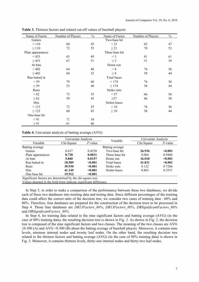
In Step 1, to achieve the goal of splitting factors and batting data, we let the statistical mean be used as

the cut-off value for each of the thirteen attributes, respectively. A summary of the thirteen factors in the

database is shown in Table 3, which contains the result of our splitting factors of Step 1. According to

these splitting values, we construct a new database DB13Factors containing thirteen attributes with

categorical values and one new added attribute AVG with class values A or B. Based on the cut-off value

determined in Table 3, the baseball data of 132 baseball player is rewritten by the related mapping rule.

For example, the statistical mean of games (G) is 110. A baseball player with the number of games (G) is

130, the mapped result of attribute G will be 1. (Note that for games (G) ≥110, we let G be value 1, and

for games (G) <110, we let G be value 2.)

Next, in Step 2, to analyze the significant factor, we use the rewritten data as the input data for the chi-

square test. The P-value from the chi-square test for batting average (AVG) is shown in Table 4, where

values denoted in the bold form indicate the significant difference. By univariate analysis, the nine

factors including PA, AB, RBI, R, H, 1B, 2B, HR, and TB are significant factors for batting average

(AVG). As shown in Table 4, the resulting nine significant factors denoted in the bold forms are those

factors which satisfy the condition of the P-value <0.05. That is, there are four insignificant factors. We

filter out the rewritten data by deleting four insignificant attributes, games (G), three-base hit (3B), strike

outs (SO), stolen bases (SB) and related data. Up to this point, we concern two databases, DB13Factors

which contains thirteen factors with categorical values 1/2 and attributes AVG with class values A/B, and

DBSignificantFactors which does not contain those four insignificant factors and related data. That is, the

DBSignificantFactors contains only nine significant factors and related data.


7

Table 3. Thirteen factors and related cut-off values of baseball players

Name of Factor Number of Players % Name of Factor Number of Players %

Games Two-base hit

< 110 60 45 < 21 62 47

≥ 110 72 55 ≥ 21 70 53

Plate appearances Three-base hit

< 453 65 49 < 3 81 61

≥ 453 67 51 ≥ 3 51 39

At bats Home run

< 402 64 48 < 8 74 56

≥ 402 68 52 ≥ 8 58 44

Run batted in Total bases

< 59 79 60 < 174 74 56

≥ 59 53 40 ≥ 174 58 44

Runs Strike outs

< 62 73 55 < 57 66 50

≥ 62 59 45 ≥57 66 50

Hits Stolen bases

< 123 72 55 < 10 74 56

≥ 123 60 45 ≥ 10 58 44

One-base hit

< 91 71 54

≥ 91 61 46

Table 4. Univariate analysis of batting average (AVG)

Univariate Analysis Univariate Analysis

Variable Chi-Square P-value Variable

Chi-Square P-value

Batting average Batting average

Games 0.637 0.4250 Two-base hit 26.936 <0.001

Plate appearances 8.738 0.0031 Three-base hit 0.004 0.9480

At bats 5.840 0.0157 Home run 16.018 <0.001

Run batted in 18.589 <0.001 Total bases 41.831 <0.001

Runs 30.930 <0.001 Strike outs 0.122 0.7266

Hits 41.149 <0.001 Stolen bases 0.862 0.3531

One-base hit 19.912 <0.001

Significant factors are determined by the chi-square test.

Values denoted in the bold form indicate significant difference.

In Step 3, in order to make a comparison of the performance between these two databases, we divide

each of these two databases into training data and testing data. Since different percentages of the training

data could affect the correct ratio of the decision tree, we consider two cases of training data : 60% and

80%. Therefore, four databases are prepared for the construction of the decision trees to be processed in

Step 4. Those four databases are DB13Factors_60%, DB13Factors_80%, DBSignificantFactors_60%

and DBSignificantFactors_80%.

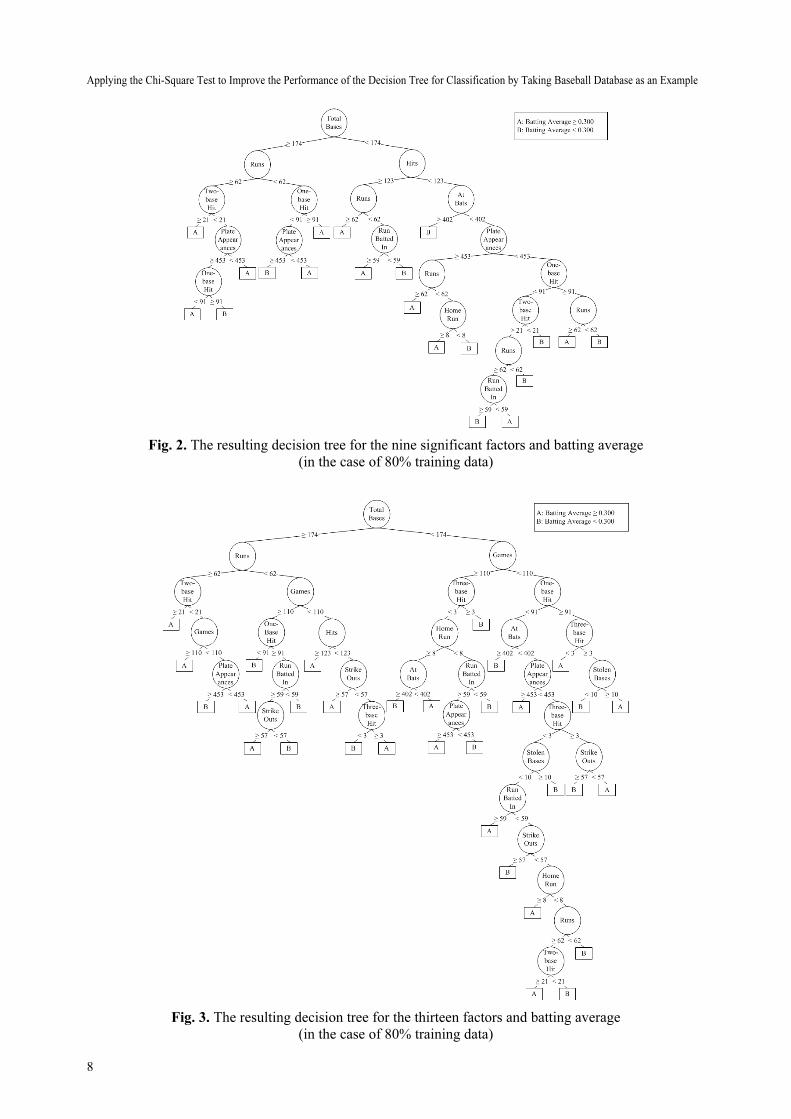
In Step 4, for training data related to the nine significant factors and batting average (AVG) (in the

case of 80% training data), the resulting decision tree is shown in Fig. 2. As shown in Fig. 2, the decision

tree is composed of the nine significant factors and two classes. The meaning of the two classes are AVG

≥0.300 (A) and AVG <0.300 (B) about the batting average of baseball players. Moreover, it contains nine

levels, nineteen internal nodes and twenty leaf nodes. On the other hand, the resulting decision tree

related to the thirteen factors and batting average (AVG) (in the case of 80% training data) is shown in

Fig. 3. Moreover, it contains thirteen levels, thirty-one internal nodes and thirty-two leaf nodes.


8

Fig. 2. The resulting decision tree for the nine significant factors and batting average

(in the case of 80% training data)

Fig. 3. The resulting decision tree for the thirteen factors and batting average



9

For the case of using 60% training data, the resulting decision tree with nine factors is the same as the

decision tree of the case of using 80% training data as shown in Fig. 2. Moreover, the resulting decision

tree with the thirteen factors is also the same as the decision tree of the case of using 80% training data as

shown in Fig. 3. The detailed discussion about the performance of those two classification trees shown in

Fig. 2 and Fig. 3 in Step 5 is described in the next section.

4 Performance

In the database of the 132 baseball players, all of the baseball players whose AVG are greater than or

equal to 372 (120 games multiplied by 3.1) are concerned in this study. As stated before, we care about

the performance for the same decision tree construction algorithm (for example, the C4.5 algorithm)

with/without the proposed preprocessing step which makes use of the P-value. Based on such baseball

data described in Section 3, Table 4 shows the resulting significant factors decided by the chi-square test,

which are the factors with the P-value less than 0.05. The nine factors including PA, AB, RBI, R, H, 1B,

2B, HR, and TB are significant factors for batting average (AVG).

Fig. 2 shows the resulting decision tree (in the case of 80% training data) which contains the nine

significant factors for deciding batting average (AVG). According to the resulting decision tree, we can

classify the batting performance by even only three factors in this study. For example, our resulting

decision tree shows that baseball players with TB ≥174, R ≥62, and 2B ≥21 can be immediately classified

to AVG ≥0.300 as shown in Fig. 2. In this example, the meaning of the result is that a baseball player

whose TB, R, and 2B are good enough will be classified into an excellent batting average (AVG) denoted

as class A. Table 5 shows a comparison of the classification by three factors between the decision tree

concerning the nine significant factors and the decision tree concerning the thirteen original factors. In

our resulting decision tree of the nine significant factors, we find that the resulting decision tree contains

four classification rules which need only concerning three factors. However, for the decision tree created

from the database with thirteen factors, we find only two classification rules decided by three factors.

Consequently, for the performance in terms of the processing time of the classification, the decision tree

with nine factors is more efficient than the one with thirteen original factors.

Table 5. A comparison of the classification by three factors

Factors Count Rule AVG Classification

TB ≥174, R ≥62, and 2B ≥21 ≥300 A

TB ≥174, R <62, and 1B ≥91 ≥300 A

TB <174, H ≥123, and R ≥62 ≥300 A Nine Factors 4

TB <174, H <123, and AB ≥402 <300 B

TB ≥174, R ≥62, and 2B ≥21 ≥300 A Thirteen Factors 2

TB <174, G ≥110, and 3B ≥3 <300 B

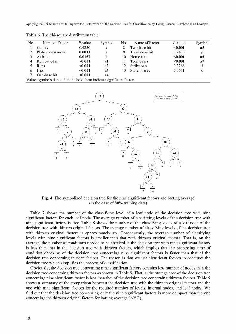
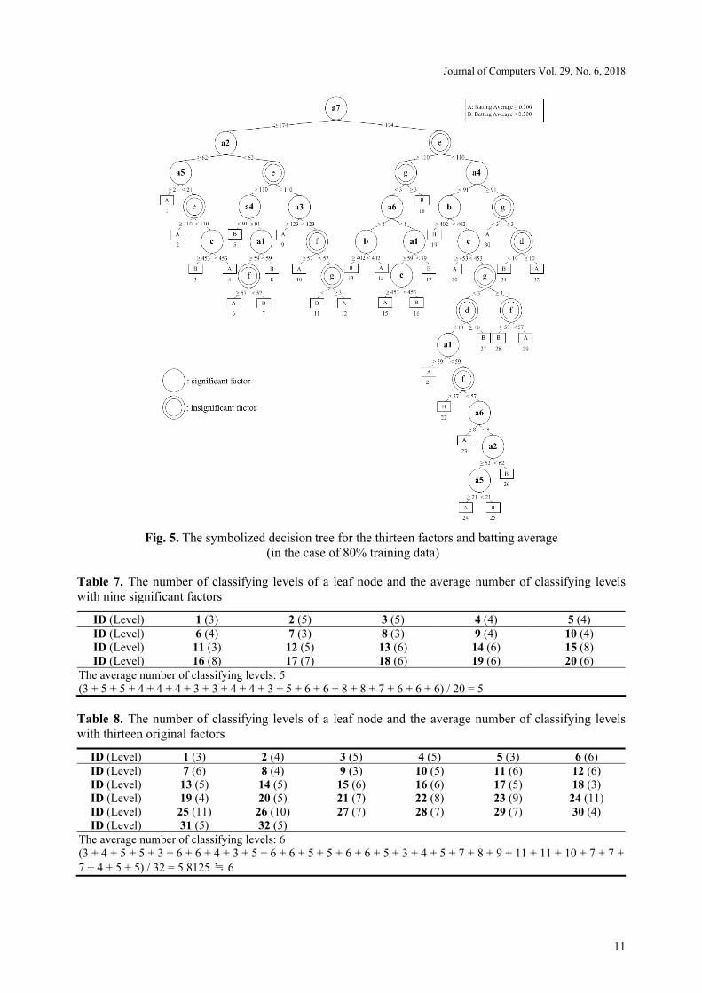
Table 6 shows the transformation from thirteen factors to symbols. Symbols a, b and c represent those

factors which are significant factors (the P-value <0.05). Here, we let factors be denoted in the

alphabetical order (i.e., the Symbol column) according to the increasing order of the P-values. For factors

with the same P-value, we add one integer to distinguish them. Furthermore, symbols d, e, f and g

represent those factors which are not significant factors. We use these symbols to redraw Fig. 2 and Fig.

3 as shown in Fig. 4 and Fig. 5, respectively. In terms of the result of the decision tree, we find a

relationship between the P-value and the decision tree in this study. In the decision tree concerning nine

significant factors shown in Fig. 4, the top three levels contain six nodes with the P-value <0.05 among

total seven nodes. While in the decision tree concerning thirteen factors shown in Fig. 5, the top three

levels contain only four significant factors. Moreover, for the other three nodes in the top three levels of

the decision tree concerning thirteen factors shown in Fig. 5, they are insignificant factors. These

observations indicate that the decision tree concerning only significant factors can strongly affect the

processing time of the prediction, since the case of the most significant factor (i.e., the factor with the

minimum P-value) is concerned first can reduce the number of conditions (i.e., levels) to be decided.


10

Table 6. The chi-square distribution table

No. Name of Factor P-value Symbol No. Name of Factor P-value Symbol

1 Games 0.4250 e 8 Two-base hit <0.001 a5

2 Plate appearances 0.0031 c 9 Three-base hit 0.9480 g

3 At bats 0.0157 b 10 Home run <0.001 a6

4 Run batted in <0.001 a1 11 Total bases <0.001 a7

5 Runs <0.001 a2 12 Strike outs 0.7266 f

6 Hits <0.001 a3 13 Stolen bases 0.3531 d

7 One-base hit <0.001 a4

Values/symbols denoted in the bold form indicate significant factors.

Fig. 4. The symbolized decision tree for the nine significant factors and batting average


Table 7 shows the number of the classifying level of a leaf node of the decision tree with nine

significant factors for each leaf node. The average number of classifying levels of the decision tree with

nine significant factors is five. Table 8 shows the number of the classifying levels of a leaf node of the

decision tree with thirteen original factors. The average number of classifying levels of the decision tree

with thirteen original factors is approximately six. Consequently, the average number of classifying

levels with nine significant factors is smaller than that with thirteen original factors. That is, on the

average, the number of conditions needed to be checked in the decision tree with nine significant factors

is less than that in the decision tree with thirteen factors, which implies that the processing time of

condition checking of the decision tree concerning nine significant factors is faster than that of the

decision tree concerning thirteen factors. The reason is that we use significant factors to construct the

decision tree which simplifies the process of classification.

Obviously, the decision tree concerning nine significant factors contains less number of nodes than the

decision tree concerning thirteen factors as shown in Table 9. That is, the storage cost of the decision tree

concerning nine significant factor is less than that of the decision tree concerning thirteen factors. Table 9

shows a summary of the comparison between the decision tree with the thirteen original factors and the

one with nine significant factors for the required number of levels, internal nodes, and leaf nodes. We

find out that the decision tree concerning only the nine significant factors is more compact than the one

concerning the thirteen original factors for batting average (AVG).


11

Fig. 5. The symbolized decision tree for the thirteen factors and batting average


Table 7. The number of classifying levels of a leaf node and the average number of classifying levels

with nine significant factors

ID (Level) 1 (3) 2 (5) 3 (5) 4 (4) 5 (4)

ID (Level) 6 (4) 7 (3) 8 (3) 9 (4) 10 (4)

ID (Level) 11 (3) 12 (5) 13 (6) 14 (6) 15 (8)

ID (Level) 16 (8) 17 (7) 18 (6) 19 (6) 20 (6)

The average number of classifying levels: 5

(3 + 5 + 5 + 4 + 4 + 4 + 3 + 3 + 4 + 4 + 3 + 5 + 6 + 6 + 8 + 8 + 7 + 6 + 6 + 6) / 20 = 5

Table 8. The number of classifying levels of a leaf node and the average number of classifying levels

with thirteen original factors

ID (Level) 1 (3) 2 (4) 3 (5) 4 (5) 5 (3) 6 (6)

ID (Level) 7 (6) 8 (4) 9 (3) 10 (5) 11 (6) 12 (6)

ID (Level) 13 (5) 14 (5) 15 (6) 16 (6) 17 (5) 18 (3)

ID (Level) 19 (4) 20 (5) 21 (7) 22 (8) 23 (9) 24 (11)

ID (Level) 25 (11) 26 (10) 27 (7) 28 (7) 29 (7) 30 (4)

ID (Level) 31 (5) 32 (5)

The average number of classifying levels: 6

(3 + 4 + 5 + 5 + 3 + 6 + 6 + 4 + 3 + 5 + 6 + 6 + 5 + 5 + 6 + 6 + 5 + 3 + 4 + 5 + 7 + 8 + 9 + 11 + 11 + 10 + 7 + 7 +

7 + 4 + 5 + 5) / 32 = 5.8125 ≒ 6


12

Table 9. A summary of the storage cost of the decision tree with nine significant factors and thirteen

original factors

No. Number of Factors Level Internal Node Leaf Node Number of Nodes

1 Nine Factors 9 19 20 39

2 Thirteen Factors 13 31 32 63

After classifying testing data, the correct ratio can be computed from WEKA automatically. We make

a comparison of the correct ratio with four input databases including DB13Factors_60%, DB13Factors_

80%, DBSignificantFactors_60% and DBSignificantFactors_80% as shown in Fig. 6. From Fig. 6, we

show that the correct ratio of the decision tree concerning only nine significant factors is higher than that

of the decision tree concerning thirteen factors both in the case of 60% and 80% training data. By

pruning the insignificant factors, we can avoid constructing the inaccurate decision tree from unnecessary

data. Because the insignificant factors interfere with the decision tree for classification. However, those

pruning strategies stated in [35] are used during the construction step of the decision tree. But our method

makes uses of the P-value to decide the significant factors before constructing the decision tree.

Therefore, our method can be used as the preprocessing step to prune insignificant factors and

unnecessary data, i.e., a kind of pruning strategy, before constructing the decision tree.

Fig. 6. A comparison of the correct ratio between the decision tree concerning nine significant factors

and the decision tree concerning thirteen factors under different percentages of training data

Moreover, the difference of the correct ratio between DBSignificantFactors_80% and DB13Factors_

80% is 3.85% as shown in Table 10. That is, the correct ratio of DBSignificantFactors_80% is higher

than that of DB13Factors_80%. Similarly, the correct ratio of DBSignificantFactors_60% is higher than

that of DB13Factors_60%. The reason is that insignificant factors exist in the database

DB13Factors_60% and DB13Factors_80%, which will interfere with classifying data in the decision tree.

In this study, the significant factors are confirmed by the chi-square test before. For the decision tree

concerning nine significant factors, there is not much disorderly data to interfere with classifying data

through Step 2. By pruning insignificant factors, the classification of the decision tree is reliable and the

structure is compact. Furthermore, the difference of the correct ratio between DBSignificantFactors_80%

and DBSignificantFactors_60% for the case of concerning only nine significant factors is 12.84%. It

means that the correct ratio of 80% training data is higher than 60% training data in the case of the

decision tree concerning only nine significant factors. Similarly, the correct ratio of DB13Factors_80% is

higher than that of DB13Factors_60% for the case of the decision tree concerning thirteen factors. The

result means that when the amount of training data increases, the correct ratio increases. However, the

increasing percentage from 60% training data to 80% training data of our decision tree concerning nine

significant factors is larger than that of the decision tree concerning thirteen factors. The reason is that

when the amount of input training data becomes large, the decision tree will become a steady trend to

classify data. That is, the amount of the training data for constructing the decision tree will affect the

accuracy of prediction of the resulting classification tree. However, the increment of the accuracy from

DBSignificant_60% to DBSignificant_80% is larger than that from DB13Factors_60% to DB13Factors_


13

80%. The main reason is that the training data of DB13Factors_80% contains many insignificant factors

and related data which could interfere with the prediction.

Table 10. A summary of the correct ratio between the decision tree with nine significant factors and

thirteen original factors

No. Name of Factors 80% Training Data 60% Training Data Difference

1 Nine Factors 80.7692% 67.9245% 12.8447%

2 Thirteen Factors 76.9231% 66.0377% 10.8854%

Difference 3.8461% 1.8868%

5 Conclusion

In this paper, we have proposed a method which applies the P-value from the chi-square test (i.e., the

significant factor) to analyzing the relationship between the factor and the class and then construct a

compact decision tree. We have used baseball database as an example to illustrate our idea. The original

baseball database concerning the batting average denoted as AVG has thirteen factors. After we have

used the chi-square test concerning the relationship between each of thirteen factors and AVG, we have

gotten nine significant factors strongly related to AVG. Then, we have used those nine significant factors

and related data to construct the decision tree. We have observed that the decision tree concerning only

significant factors can strongly affect the processing time of the prediction, since the case that the most

significant factor (i.e., the factor with the minimum P-value) is concerned first can reduce the number of

conditions (i.e., levels) to be decided. This property also affects the average number of conditions needed

to be checked, the storage cost and the accuracy of prediction. From our performance study, we have

shown that our decision tree concerning only nine significant factors can provide less storage cost, faster

prediction time (due to the less average number of levels of the decision tree) and higher degree of

accuracy for data classification than the decision tree concerning the original thirteen factors related to

AVG, both in the cases of using 80% and 60% training data. In fact, our proposed method can be applied

to any other database for an extra attribute with a class value. The contribution of our method can be used

as the preprocessing step to prune insignificant factors and unnecessary data before constructing the

decision tree. However, all the related values of concerned factors must be converted to categorical

values first, such a task needs to decide the cut-off value for continuous values and may take long time.

How to efficiently finish such a task is the possible research direction.

Acknowledgements

This work was supported by the Ministry of Science and Technology, R.O.C. [grant numbers 101-2221-

E-110-091-MY2].

References

[1] C.H. Kang, T.J. Yu, H.H. Hsieh, J.W. Yang, K. Shu, C.C. Huang, P.H. Chiang, Y.L. Shiue, The development of bladder

tumors and contralateral upper urinary tract tumors after primary transitional cell carcinoma of the upper urinary tract,

Cancer 98(8)(2003) 1620-1626.

[2] C.E. Li, C.S. Chien, Y.C. Chuang, Y.I. Chang, H.P. Tang, C.H. Kang, Chronic kidney disease as an important risk factor for

tumor recurrences, progression and overall survival in primary non-muscle invasive bladder cancer, International Urology

and Nephrology 48(6)(2016) 993-999.

[3] G.-J. Wang, C. Xie, M. Lin, H.E. Stanley, Stock market contagion during the global financial crisis: a multiscale approach,

Finance Research Letters 22(2017) 163-168.

[4] E.T. Hébert, E.A. Vandewater, M.S. Businelle, M.B. Harrell, S.H. Kelder, C.L. Perry, Feasibility and reliability of a mobile


14

tool to evaluate exposure to tobacco product marketing and messages using ecological momentary assessment, Addictive

Behaviors 73(2017) 105-110.

[5] A. Jiménez, M.C. Monroe, N. Zamora, J. Benayas, Trends in environmental education for biodiversity conservation in Costa

Rica, Environment, Development and Sustainability 19(1)(2017) 221-238.

[6] C.-C. Hsu, Y.-M. Wang, C.-R. Huang, F.-J. Sun, J.-P. Lin, P.-K. Yip, S.-I. Liu, Sustained benefit of a psycho-educational

training program for dementia caregivers in Taiwan, Computer & Education 11(1)(2017) 31-35.

[7] G. Alberti, F.M. Iaia, E. Arcelli, L. Cavaggioni, Goal scoring patterns in major european soccer leagues, Sport Science for

Health 9(3)(2013) 151-153.

[8] A. Marques, U. Ekelund, L.B. Sardinh, Associations between organized sports participation and objectively measured

physical activity, sedentary time and weight status in youth, Journal of Science and Medicine in Sport 19(2)(2016) 154-157.

[9] M. Lochbaum, J. Gottardy, A meta-analytic review of the approach-avoidance achievement goals and performance

relationships in the sport psychology literature, Journal of Sport and Health Science 4(2)(2015) 164-173.

[10] M.J.A. Berry, G.S. Linoff, Data Mining Techniques: For Marketing, Sales, and Customer Support, John Wiley & Sons,

New York, 1997.

[11] Y. Zhao, Y. Zhang, Comparison of decision tree methods for finding active objects, Advances in Space Research

41(12)(2008) 1955-1959.

[12] A. Carmona-Bayonas, P. Jiménez-Fonseca, C. Font, F. Fenoy, R. Otero, C. Beato, J.M. Plasencia, M. Biosca, M. Sánchez,

M. Benegas, D. Calvo-Temprano, D. Varona, L. Faez, I. de la Haba, M. Antonio, O. Madridano, M.P. Solis, A.

Ramchandani, E. Castañón, P.J. Marchena, M. Martin, F. Ayala delaPena,�� V. Vicente, Predicting serious complications in

patients with cancer and pulmonary embolism using decision tree modelling: the EPIPHANY Index, British Journal of

Cancer 116(2017) 994-1001.

[13] L. Mage, N. Baati, A. Nanchen, F. Stoessel, Th. Meyer, A systematic approach for thermal stability predictions of

chemicals and their risk assessment: pattern recognition and compounds classification based on thermal decomposition

curves, Process Safety and Environmental Protection 110(2017) 43-52.

[14] M. Fleischman, B. Roy, D. Roy, Temporal feature induction for baseball highlight classification, in: Proc. the 15th ACM

International Conference on Multimedia, MM-15, 2007.

[15] Y.-I. Chang, C.-C. Wu, J.-H. Shen, C.-H. Chen, Data classification based on the class-rooted FP-Tree approach, in: Proc.

IEEE International Conference on Complex, Intelligent and Software Intensive Systems, CISIS, 2009.

[16] R. Agrawal, R. Srikant, Fast algorithms for mining association rules in large databases, in: Proc. the 20th International

Conference on Very Large Databases, VLDB-20, 1994.

[17] J.R. Quinlan, C4.5: programs for machine learning, Morgan Kaufmann, San Francisco, CA, 1993.

[18] J.R. Quinlan, Improved use of continuous attributes in C4.5, Journal of Artificial Intelligence Research 4(1)(1996) 77-90.

[19] W. Meredith, Measurement invariance, factor analysis and factorial invariance, Psychometrika 58(4)(1993) 525-543.

[20] D.W.K. Andrew, Chi-square diagnostic tests for econometric models: introduction and applications, Journal of

Econometrics 37(1)(1988) 135-156.

[21] M.L. McHugh, The chi-square test of independence, Biochemia Medica 23(2)(2013) 143-149.

[22] W.-H. Au, K.C.C. Chan, X. Yao, A novel evolutionary data mining algorithm with applications to churn prediction, IEEE

Transactions on Evolutionary Computation 7(6)(2003) 532-545.

[23] J.R. Quinlan, Introduction of decision trees, Machine Learning 1(1)(1986) 81-106.


15

[24] M. Suknovic, B. Delibasic, M. Jovanovic, M. Vukicevic, D. Becejski-Vujaklija, Z. Obradovic, Reusable components in

decision tree induction algorithms, Computational Statistics 27(1)(2011) 127-148.

[25] World Baseball Softball Confederation, World Baseball Softball Confederation History. <http://www.wbsc.org/wbsc-

history/>, 2017 (accessed 21 June 2017).

[26] Chinese Professional Baseball League, Chinese professional baseball league games. <http://www.cpbl.com.tw/eng/

structures>, 2017 (accessed 21 June 2017).

[27] Chinese Professional Baseball League, Chinese professional baseball league players. <http://www.cpbl.com.tw/stats/all.

html>, 2017 (accessed 21 June 2017).

[28] Major League Baseball, Major league baseball 2017 official rules. <http://mlb.mlb.com/mlb/official_info/official_

rules/official_rules.jsp>, 2017 (accessed 21 June 2017).

[29] Chinese Professional Baseball League, Chinese Professional Baseball League 2017 Official Rules. <http://www.cpbl.

com.tw/footer/rule/09>, 2017 (accessed 21 June 2017).

[30] M.C. Jadud, B. Dorn, Aggregate compilation behavior: findings and implications from 27,698 users, in: Proc. the 11th

Annual International Conference on International Computing Education Research, ICER-11, 2015.

[31] J. Mingers, An empirical comparison of pruning methods for decision tree induction, Machine Learning 4(2)(1989) 227-

243.

[32] T.C.E. Cheng, D.Y.C. Lam, A.C.L. Yeung, Adoption of internet banking: an empirical study in Hong Kong, Decision

Support Systems 42(3)(2006) 1558-1572.

[33] E. Frank, M. Hall, L. Trigg, G. Holmes, I.H. Witten, Data mining in bioinformatics using Weka, Bioinformatics

20(15)(2004) 2479-2481.

[34] R. Conforti, M. Leoni, M.L. Rosa, W.M.P. van der Aalst, A.H.M. ter Hofstede, A recommendation system for predicting

risks across multiple business process instances, Decision Support Systems 69(2015) 1-19.

[35] M. Bohanec, I. Bratko, Trading accuracy for simplicity in decision trees, Machine Learning 15(3)(1994) 223-250.

Documents

Applying the Chi-Square Test to Improve the Performance of