1

Applying Swarm Rule Abstraction to a WirelessSensor Network Domain

Peter A. Hamilton

Abstract—Rule abstraction is a powerful tool for modelingabstract behaviors in swarm systems. The research presentedin this paper examines the application of rule abstraction tothe wireless sensor network domain. I specifically analyze thepotential of rule abstraction to accurately model and control theconnectivity, coverage, and density of a simple sensor network. Inthis paper, I also present a simulation tool developed to facilitatethe discovery and creation of new abstract rules and discusspreliminary experimental results that will hopefully lead to thedevelopment of new abstract rules.

Index Terms—network layout, optimization, rule abstraction,swarm, simulator, wireless sensor network

I. INTRODUCTION

Planning the optimal layout and organization of a wirelesssensor network (WSN) can be a difficult task. Specific knowl-edge about the environment must be gathered and analyzedbefore planning can begin, and depending upon the applica-tion, the best locations for gathering data must be identified[7]. Various network characteristics must also be taken intoconsideration. For example, how much target area coverageis required to obtain an acceptable sampling of data? Howdoes the physical layout affect possible weaknesses in thenetwork, such as energy consumption or network congestion?These questions inspire improvements to the network layout,but modifications may change other network characteristics,requiring additional modifications. It is possible for an un-ending cycle of modifications to result from this process,complicating network design. Ideally, it would be helpful tounderstand how different network characteristics are relatedand how manipulating one characteristic will affect the others.

To address this problem, I propose applying a new form ofswarm intelligence, known as rule abstraction, as an organiza-tional method for WSN design [8]. To help in the applicationof rule abstraction, I have designed and implemented a WSNsimulator that integrates network and swarm functionality,enabling user control of the swarm while facilitating analysisof network characteristics.

II. BACKGROUND & RELATED WORK

A. Swarm IntelligenceSwarm intelligence is a field of artificial intelligence that

models the intelligent behavior observed in creature swarmsby using multiagent systems [2]. Many organisms demonstrateswarm behavior, including various species of birds, fish, andinsects. Swarm behavior can result in unexpected yet orga-nized emergent behaviors that make the creature swarm morerobust. For example, fish swarm in schools for protection frompredators. Ants lay pheromone trails while searching for food,

reinforcing the most traveled paths when a food source islocated, thereby guiding more workers to the source.

The agents used to model a swarm are often autonomousand self-organizing, following a predefined set of low-levelrules that govern individual behavior. Each rule has a specificweight factor that determines the magnitude of its influenceon an agent’s actions. As each agent follows the rule set,the overall behavior of the swarm may coordinate to producemore complicated emergent behaviors. A traditional exampleof emergent behavior is flocking. Demonstrated by Reynolds,flocking is produced by following three low-level rules: avoidcolliding with neighboring agents (AvoidCollision), move to-wards the center of mass of neighboring agents (MoveToMass-Center), and move in the direction that neighboring agents aremoving (MoveWithNeighbors) [12].

First introduced in relation to cellular robotics, swarmintelligence has since been associated with multiagent systems[1] [2]. Many applications and algorithms have been developedthat utilize swarm intelligence. A common example, particleswarm optimization, is a technique where swarm agents rep-resent problem solutions for a specific problem, searching theproblem solution space for optimal solutions and, over time,moving towards the best solutions discovered [11].

B. Swarm Rule Abstraction

Swarm rule abstraction is a new swarm intelligence tech-nique that seeks to represent the emergent behaviors of aswarm system as individual rules [8]. Since emergent behav-iors are products of individual agent interactions as the agentsfollow the rule set, there is an intuitive connection between thelow-level rules, their rule weights, and the emergent behavior.The discovery of relationships between low-level and abstractrules can lead to a swarm rule hierarchy that can be usedin the development of additional abstract rules. An abstractrule, while representing a simple emergent behavior, can alsoaccept a quantifier that specifically describes how or to whatdegree the swarm should demonstrate the desired behavior.For example, the rule FormCircle() might have a parametervalue to define what the radius of the circle should be.FormCircle(60) would direct the swarm to form a circle ofradius 60.

Swarm rule abstraction is a fairly new approach to theproblem of efficient swarm control. The original work val-idating and demonstrating the concept focused primarily onsimple geometric shape formation and ant colony models [8].The FormCircle() rule was one of the first rules developedto demonstrate the ability of top-down mapping, where theabstract rule parameter is used to manipulate the low-level rule

2

weights to produce specific behavior. To create this mappingprocess, multiple experiments were conducted, measuring theresulting swarm behavior as the individual rule weights wereadjusted. A more robust process has recently been developedfor creating abstract rules, involving a systematic sampling ofsimulation data to create a top-down mapping [9]. Due to thenovelty of swarm rule abstraction, this paper is the first toconsider applying abstract rules to the WSN domain.

C. Wireless Sensor Networks

A wireless sensor network is composed of physicallydisconnected sensors that must communicate wirelessly tocollect data and coordinate activity [13]. The nature and exactspecifications of the network can vary depending upon theapplication. The traditional WSN model, originally focused onmilitary applications, involved a random distribution of sensorsthroughout the target area, in addition to one or more sinknodes. Since the network is isolated, the sensors have limitedsensing and communication capabilities as well as limitedbattery life, unless fitted with energy-generation technology(e.g., solar panels). Transmissions are multi-hop, passing alongthe most cost-effective path in the network graph from theoriginating sensor to the sink. Sink nodes are typically morepowerful then the ordinary sensors and may have greaterenergy capacity and better sensing and communicating equip-ment; they may even be physically connected to other sinknodes in the network. Sensors may be stationary or mobile, al-lowing for dynamic configurations and layouts of the networkdepending on certain events or commands. Applications ofWSNs include target detection, tracking, pursuit, and passivearea monitoring for security purposes.

In recent WSN developments, networks can be heteroge-neous, incorporating sensors with different capabilities andresources. The environment and surrounding topology can alsoaffect how the network operates: sensors at higher elevationsmay be able to communicate further, while those in valleysor surrounded by obstacles may have limited sensing range.The motion of a sensor may be outside its control, as in thecase of cell phones passing in and out of range of variouscell towers or cars travelling along a highway. These adhocnetworks must be robust to sudden changes and must be able toquickly coordinate sensor communications to preserve qualityof service.

Environment monitoring has also become an importantapplication. WSNs have been applied to monitoring wild life inisolated regions as well as passively performing temperature,atmospheric, and seismic data gathering. Networks have beenestablished to monitor glacier activity, to measure salinity andsand bank formation in coastal regions hosting wind farms,and to locate victims of an avalanche [13]. Urban areas havealso become testbeds for WSN applications; applications rangefrom tracking building power consumption to monitoringpatient activity and vital signs in hospitals [13]. As a domaincomposed of multiple cooperating entities, WSNs are ideallysuited to the swarm intelligence paradigm.

D. Swarm Intelligence and Wireless Sensor Networks

Much work has been done in applying swarm intelligenceto the optimization of sensor network performance. Particleswarm optimization has been applied to the problem of se-lecting network configurations that maximize network lifetime[15]. Groups of swarms have been designed to learn theparameters of a fuzzy-logic controller used to dictate sourcesearch strategies in an environment [4].

Ant colony models are also popular in addressing networkoptimization problems. Pheromone-based routing algorithmshave been developed that allow networks to dynamically routedata packets along paths that use sensors with the most energyresources, prolonging network lifetime and connectivity [10].Pheromone tracing has also been used to organize mobile net-works in dynamic event detection, task completion, and sleepscheduling [6]. For example, if a target is detected crossing anarea of interest, the network controller determines the numberof sensors needed to adequately track and monitor it. If thereare too few sensors in range, those present drop pheromonesto attract more sensors. The pheromones accumulate over timeif the task is left uncompleted. If the task is completed, thesensors stop laying pheromones, which disappear over time.

Applying swarm intelligence to WSN design and optimiza-tion is not a novel idea. However, due to the increasing overlapbetween the fields, there is still much research to be done andthe application of swarm rule abstraction is an appropriateextension of swarm intelligence.

III. WSN SIMULATOR

To facilitate and demonstrate the application of swarmrule abstraction to the WSN domain, I implemented a WSNsimulator that conducts network layout simulations. In thebackground, the simulator treats the network sensors as agentsin a single swarm. Due to the novelty of swarm rule abstrac-tion, no preexisting simulation tool exists that can supportboth rule abstraction and WSNs while also providing the low-level control needed to adjust the low-level rule weights. Thesimulator is implemented in Python 2.5.1.

The simulations presented have used the traditional def-inition of a wireless sensor network. Specifically, the net-work is homogeneous: all sensors have the same sensingand transmission range and all sensor agents have the samesets of rules applied to their behavior. To simplify analysis,the network environment is modeled as a two-dimensionalfeatureless Euclidean grid, with no obstacles in the environ-ment aside from the other sensor agents; also, all possiblegrid configurations are restricted to rectangular shapes, furtherlimiting environment complexity.

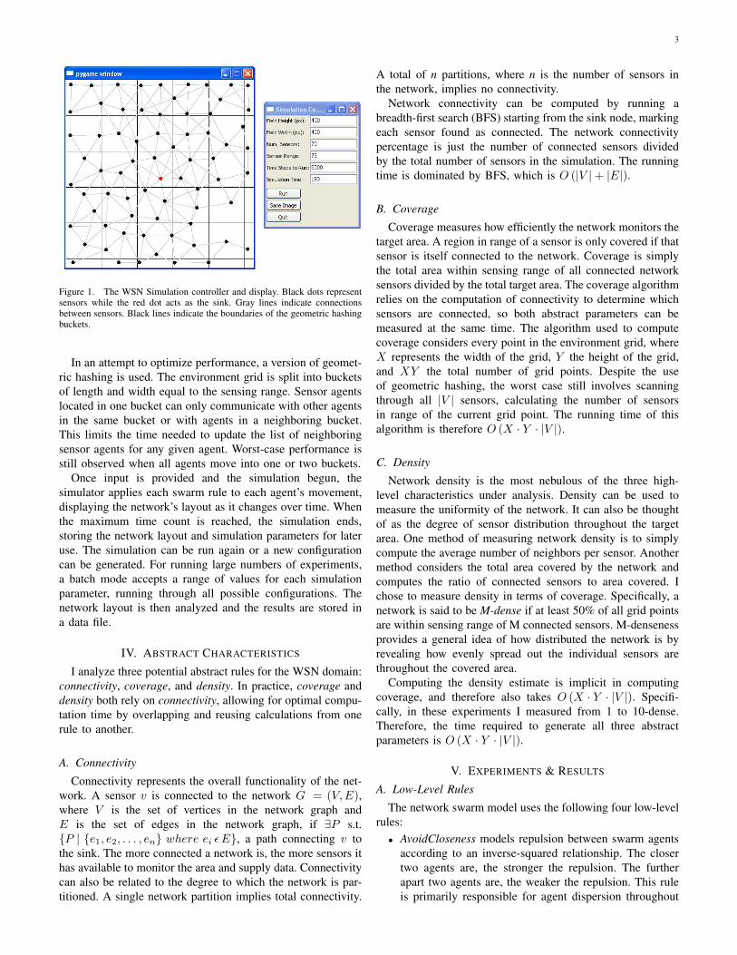
The simulator is composed of two applications: the networkparameter controller and the network layout display. The con-troller is a GUI that allows the user to specify various networkparameters, including environment grid size, the number ofsensors in the network, the sensing/transmission range of thesensors, and the number of time steps to run the simulation.The display shows the movement of the swarm over time,connecting and disconnecting sensor agents who move in andout of transmission range of each other.

3

Figure 1. The WSN Simulation controller and display. Black dots representsensors while the red dot acts as the sink. Gray lines indicate connectionsbetween sensors. Black lines indicate the boundaries of the geometric hashingbuckets.

In an attempt to optimize performance, a version of geomet-ric hashing is used. The environment grid is split into bucketsof length and width equal to the sensing range. Sensor agentslocated in one bucket can only communicate with other agentsin the same bucket or with agents in a neighboring bucket.This limits the time needed to update the list of neighboringsensor agents for any given agent. Worst-case performance isstill observed when all agents move into one or two buckets.

Once input is provided and the simulation begun, thesimulator applies each swarm rule to each agent’s movement,displaying the network’s layout as it changes over time. Whenthe maximum time count is reached, the simulation ends,storing the network layout and simulation parameters for lateruse. The simulation can be run again or a new configurationcan be generated. For running large numbers of experiments,a batch mode accepts a range of values for each simulationparameter, running through all possible configurations. Thenetwork layout is then analyzed and the results are stored ina data file.

IV. ABSTRACT CHARACTERISTICS

I analyze three potential abstract rules for the WSN domain:connectivity, coverage, and density. In practice, coverage anddensity both rely on connectivity, allowing for optimal compu-tation time by overlapping and reusing calculations from onerule to another.

A. ConnectivityConnectivity represents the overall functionality of the net-

work. A sensor v is connected to the network G = (V,E),where V is the set of vertices in the network graph andE is the set of edges in the network graph, if !P s.t.{P | {e1, e2, . . . , en} where ei ! E}, a path connecting v tothe sink. The more connected a network is, the more sensors ithas available to monitor the area and supply data. Connectivitycan also be related to the degree to which the network is par-titioned. A single network partition implies total connectivity.

A total of n partitions, where n is the number of sensors inthe network, implies no connectivity.

Network connectivity can be computed by running abreadth-first search (BFS) starting from the sink node, markingeach sensor found as connected. The network connectivitypercentage is just the number of connected sensors dividedby the total number of sensors in the simulation. The runningtime is dominated by BFS, which is O (|V | + |E|).

B. CoverageCoverage measures how efficiently the network monitors the

target area. A region in range of a sensor is only covered if thatsensor is itself connected to the network. Coverage is simplythe total area within sensing range of all connected networksensors divided by the total target area. The coverage algorithmrelies on the computation of connectivity to determine whichsensors are connected, so both abstract parameters can bemeasured at the same time. The algorithm used to computecoverage considers every point in the environment grid, whereX represents the width of the grid, Y the height of the grid,and XY the total number of grid points. Despite the useof geometric hashing, the worst case still involves scanningthrough all |V | sensors, calculating the number of sensorsin range of the current grid point. The running time of thisalgorithm is therefore O (X · Y · |V |).

C. DensityNetwork density is the most nebulous of the three high-

level characteristics under analysis. Density can be used tomeasure the uniformity of the network. It can also be thoughtof as the degree of sensor distribution throughout the targetarea. One method of measuring network density is to simplycompute the average number of neighbors per sensor. Anothermethod considers the total area covered by the network andcomputes the ratio of connected sensors to area covered. Ichose to measure density in terms of coverage. Specifically, anetwork is said to be M-dense if at least 50% of all grid pointsare within sensing range of M connected sensors. M-densenessprovides a general idea of how distributed the network is byrevealing how evenly spread out the individual sensors arethroughout the covered area.

Computing the density estimate is implicit in computingcoverage, and therefore also takes O (X · Y · |V |). Specifi-cally, in these experiments I measured from 1 to 10-dense.Therefore, the time required to generate all three abstractparameters is O (X · Y · |V |).

V. EXPERIMENTS & RESULTS

A. Low-Level RulesThe network swarm model uses the following four low-level

rules:• AvoidCloseness models repulsion between swarm agents

according to an inverse-squared relationship. The closertwo agents are, the stronger the repulsion. The furtherapart two agents are, the weaker the repulsion. This ruleis primarily responsible for agent dispersion throughout

4

the environment grid. The parameter of this rule variesthe strength of the repulsion [8].

• MoveToCenter is a conditional rule that a swarm agentfollows when it has no neighbors. By convention, theagent will move toward the center of the environment gridin an attempt to find and connect with other agents. Sincethe network sink is always located near the center, theswarm agent will eventually connect with other agents,provided that the magnitude of the sensing/transmissionrange is reasonable. Note that this does not imply that theagent will be connected to the network. It is possible fora small group of agents to connect in an isolated regionof the environment grid but not be connected to the sink.Since these agents have neighbors, they are never pulledto the center and may never connect. This rule is usedprimarily to connect as much of the network as possibleduring simulation. The parameter of this rule varies thespeed at which an isolated agent moves to the center ofthe grid.

• Slowdown is a simple mechanical rule that bounds themaximum speed an agent can attain during simulation.If not applied, the swarm tends to cyclic instability andnever reaches equilibrium. The parameter of this rulevaries the slowdown rate. For these experiments, thisparameter value is set to 0.22.

• StayInBorders is a simulation-specific rule that preventsthe sensor agents from moving outside of the target area.When an agent moves within a specific range of thearea border, a repulsive force is applied, pushing theagent away from the border. If the specified range istoo large, agents are constantly pushed around and noequilibrium is reached. If the range is too small, an agentwith high velocity can push through the repulsion andescape the environment, forever isolated from the swarm.The parameter of this rule varies the repulsion when inrange of the border. For our experiments, the border rangeis set to 10 pixels and the parameter value to 1.0.

B. Experiment Setup

In the experimental network layouts, the AvoidClosenessvalues were chosen from the set {0, 1, 10, 20, 40, 60, 80,100} and the MoveToCenter values from {0, 0.001, 0.002,0.003, 0.004}. The grid sizes are {300, 400, 500} and thesensor count and range magnitude are both {50, 60, 70, 80,90, 100}. All combinations of these parameter values weretested with 20 runs for each configuration, each with randominitial network layouts to ensure statistically valid results. Theaverage of the results for each set of 20 was then calculatedalong with a corresponding 95% confidence interval (CI). Theresults for specific data sets are provided in Appendix A. Ineach data table in Appendix A, the CIs are represented by theoffset, x, from the mean of the characteristic being measured.To calculate the actual CI, simply add and subtract the offsetfrom the mean, yielding (mean" x, mean + x).

The primary goal of these experiments is to reveal theeffects of both the environment and swarm parameters onnetwork connectivity, coverage, and density. By demonstrating

that the swarm parameters can yield results comparable tolayouts with excessive numbers of sensors or transmissioncapability, these experiments reveal the power and potentialof rule abstraction.

C. Graphs & Analysis

Due to the amount of data generated in these experiments,only a small portion can be presented here. To simplify analy-sis, five different data sets were selected and the correspondingresults for connectivity, coverage, and density graphed. Thefirst two data sets demonstrate the effects of the network andenvironment parameters (grid size, no. sensors, and sensingand transmission range) on the network while the other threedata sets reveal the effects of the swarm parameters (Avoid-Closeness factor and MoveToCenter factor) on the network.The parameters not listed in each data set serve as axes forthe data graphs. The data sets selected are:

• Grid Size = 300, No. Sensors = 50, AvoidClosenessFactor = 0

• Grid Size = 500, Range = 100, AvoidCloseness Factor =0

• Grid Size = 400, No. Sensors = 50, Range = 50• Grid Size = 400, No. Sensors = 70, Range = 70• Grid Size = 500, No. Sensors = 60, Range = 60

See Appendix A for the data tables corresponding to thegraphs. For full results see the project website1.

Each graph displays the magnitude of the CI offset for eachdata point, in addition to the average characteristic value ateach data point. The offset magnitude is represented by agray-scale shading of the xy-plane underneath each point; thedarker the shade of a grid cell, the larger the magnitude ofthe CI offset for the corresponding point. This additional datadepicts the consistency of the experiment results and furtherreveals the effects of the swarm parameters.

1) Connectivity: For network configurations with eitherlarger numbers of sensors or large transmission ranges, Iintuitively expect to see improved connectivity, regardless ofthe swarm rule factors. Figures 2 and 3 display examplesof this relationship. In Figure 2, there is a direct correlationbetween increasing range and connectivity. A single sensorcan cover more area with increasing range, also implying thatit can communicate with more sensors. As the range increases,more sensors have a direct connection to the sink, increasingnetwork connectivity. These sensors then act as intermediatenodes in the graph, allowing sensors further removed from thesink to connect, again increasing connectivity. In fact, oncethe range reaches 80 pixels, the network is almost entirelyconnected, and the corresponding CI offsets reveal that theresults are very consistent.

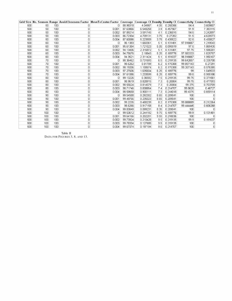
For Figure 3, there is a direct relationship between thenumber of sensors and connectivity, similar to Figure 2. Due tothe fixed size of the grid environment and the range, the resultsconverge for more configurations as the number of sensorsincreases. The variation in average connectivity still exists withlarge numbers of sensors, though average connectivity never

1http://userpages.umbc.edu/~pete5/Projects/Honors_Thesis/

5

Figure 2. Grid size = 300 pixels, No. sensors = 50, AvoidCloseness factor =0. The legend on the left defines the different ranges for the CI offset, x. Thelegend on the right associates each plot with its corresponding MoveToCenterfactor. This scheme is used for all following data graphs.

measures below 90%. From the graph, MoveToCenter factorsof 0 and 0.001 provide the most consistent results over variousnumbers of sensors.

Figure 3. Grid size = 500 pixels, Range = 100 pixels, AvoidCloseness Factor= 0.

Figures 4, 5, and 6 demonstrate the effects of Avoid-Closeness on connectivity performance. For Figure 4, theperformance improves as the AvoidCloseness factor increasesbut general performance is poor for low MoveToCenter factorvalues. The magnitude of the CI offset does not decrease asthe AvoidCloseness factor increases, unlike Figures 2 and 3.The most consistent performance that provides near optimalconnectivity for the network configuration occurs when theMoveToCenter factor is 0.002.

It is possible for a combination of network and swarmparameters to create ideal performance. In Figure 5, maximumconnectivity is achieved for very low AvoidCloseness factorvalues, and the corresponding CI intervals are as tight aspossible. The MoveToCenter factor does not make a differencebeyond an AvoidCloseness factor value of 10, conflictingwith the intuition that the MoveToCenter rule is primarilyresponsible for improving network connectivity. However, theperformance can also be interpreted as the result of excessive

Figure 4. Grid size = 400 pixels, No. sensors = 50, Range = 50 pixels:When both rule factors are 0, the network is simply a random configurationwith consistently poor performance.

numbers of sensors with adequate range flooding the targetarea. In this case, the AvoidCloseness factor would spread thesensors evenly around the grid, yielding consistent networkdensity as depicted in the corresponding density graph inFigure 15.

Figure 5. Grid size = 400 pixels, No. sensors = 70, Range = 70 pixels. TheCI offsets are as tight as possible for most of the tests in this configuration.

The connectivity performance for a smaller network in thelargest environment is displayed in Figure 6. The poor perfor-mance of the configuration with a MoveToCenter factor of 0is due to the even dispersal of the sensors with no tendencyto ensure connectivity with the sink. Overall, the MoveTo-Center factor does not affect connectivity performance. TheAvoidCloseness factor, beyond values of 10 or 20, leads tomaximum connectivity which is consistent for all remainingfactor values.

For connectivity performance, the MoveToCenter factor,while expected to greatly influence connectivity, in generalonly affects performance consistency as shown by the CIoffsets. Instead, the AvoidCloseness factor produces even dis-persal of the sensor agents, leading to better connectivity atlow factor values, depending upon the network configuration.

6

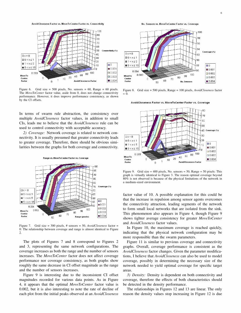
Figure 6. Grid size = 500 pixels, No. sensors = 60, Range = 60 pixels.The MoveToCenter factor value, aside from 0, does not change connectivityperformance. However, it does improve performance consistency, as shownby the CI offsets.

In terms of swarm rule abstraction, the consistency overmultiple AvoidCloseness factor values, in addition to smallCIs, leads me to believe that the AvoidCloseness rule can beused to control connectivity with acceptable accuracy.

2) Coverage: Network coverage is related to network con-nectivity. It is usually presumed that greater connectivity leadsto greater coverage. Therefore, there should be obvious simi-larities between the graphs for both coverage and connectivity.

Figure 7. Grid size = 300 pixels, # sensors = 50, AvoidCloseness factor =0: The relationship between coverage and range is almost identical to Figure2.

The plots of Figures 7 and 8 correspond to Figures 2and 3, representing the same network configurations. Thecoverage increases as both the range and the number of sensorsincreases. The MoveToCenter factor does not affect coverageperformance nor coverage consistency, as both graphs showroughly the same decrease in CI offset magnitude as the rangeand the number of sensors increases.

Figure 9 is interesting due to the inconsistent CI offsetmagnitudes recorded for various data points. As in Figure4, it appears that the optimal MoveToCenter factor value is0.002, but it is also interesting to note the rate of decline ofeach plot from the initial peaks observed at an AvoidCloseness

Figure 8. Grid size = 500 pixels, Range = 100 pixels, AvoidCloseness factor= 0.

Figure 9. Grid size = 400 pixels, No. sensors = 50, Range = 50 pixels: Thisgraph is virtually identical to Figure 3. The reason optimal coverage beyond80% is not observed is because of the physical limitations of the network ina medium-sized environment.

factor value of 10. A possible explanation for this could bethat the increase in repulsion among sensor agents overcomesthe connectivity attraction, leading segments of the networkto form small local networks that are isolated from the sink.This phenomenon also appears in Figure 4, though Figure 9shows tighter average consistency for greater MoveToCenterand AvoidCloseness factor values.

In Figure 10, the maximum coverage is reached quickly,indicating that the physical network configuration may bemore responsible than the swarm parameters.

Figure 11 is similar to previous coverage and connectivitygraphs. Overall, coverage performance is consistent as theAvoidCloseness factor changes. Given the parameter modifica-tions, I believe that AvoidCloseness can also be used to modelcoverage, possibly in determining the necessary size of thenetwork needed to yield optimal coverage for specific targetareas.

3) Density: Density is dependent on both connectivity andcoverage, therefore the effects of both characteristics shouldbe detected in the density performance.

The relationships in Figures 12 and 13 are linear. The onlyreason the density values stop increasing in Figure 12 is due

7

Figure 10. Grid size = 400 pixels, No. sensors = 70, Range = 70 pixels.Performance matches connectivity performance in Figure 5.

Figure 11. Grid size = 500 pixels, No. sensors = 60, Range = 60 pixels.Coverage performance is independent of the MoveToCenter factor and isconsistent for higher AvoidCloseness factor values.

to the fact that 10-dense was the maximum density levelmeasured in the experiments. I would expect the density tocontinue increasing with the range until any individual sensorcan cover the entire target area. At this point, the density wouldreach a maximum possible value, equal to the total number ofsensors in the network. Similarly in Figure 13, increasing thenumber of sensors in the target area will always increase thedensity, since the maximum density is dependent on the totalnumber of network sensors.

Figure 14 shows the first instance where the MoveToCenterfactor influences the density measure. A decrease in densityis observed as the AvoidCloseness factor increases, but itis most pronounced when the MoveToCenter factor value is0.001. Since density is primarily dependent on coverage, and adecrease occurs in the corresponding coverage graph in Figure9, a similar decrease in density is expected. MoveToCentervalues beyond 0.001 produce satisfactory average density,though the optimal configuration in terms of both maximumpossible density and CI offset magnitude occurs when theMoveToCenter factor value is 0.002, as in Figures 4 and 9.

The variability of average density displayed in Figure 15is at first confusing. However, the density axis shows that

Figure 12. Grid size = 300 pixels, No. sensors = 50, AvoidCloseness factor =0: Since the experiments only measure up to 10-dense, the linear relationshipbetween Density and Range is truncated. Again, swarm rule factors have noimpact on network density in this network configuration.

Figure 13. Grid size = 500 pixels, Range = 100 pixels, AvoidCloseness factor= 0.

the variability mainly occurs between 4.5-dense and 5-dense,which is actually pretty consistent. The CI offset magnitudesare also small, indicating that the measures are accurate overmultiple simulations for each configuration.

For the configuration in Figure 16, the relationship isagain obvious. Higher AvoidCloseness factor values lead togreater network dispersal throughout the environment, leadingto redundant coverage of the same areas by multiple sensors,creating higher network density. An exact CI offset for higherAvoidCloseness factor values is expected, since the sensorspread throughout the target area is confined by the areabounds and the StayInBorders rule, preserving optimal densityfor the configuration even with differing AvoidCloseness factorvalues.

For each network configuration, the density values measuredare very consistent, if not exact, making density the mostprecise of the three network characteristics measured. It alsoindicates that density is the most robust, making it resistantto changes in the swarm parameters. This could result fromthe artificial limits placed on measuring the density. However,I do not believe this to be the case because density is tied

8

Figure 14. Grid size = 400 pixels, No. sensors = 50, Range = 50 pixels:No satisfactory density is recorded when both swarm rule factors are 0, asexpected.

Figure 15. Grid size = 400 pixels, No. sensors = 70, Range = 70 pixels.While there appears to be a lot of variability in the average density measures,the density axis reveals that all values, aside from those with AvoidCloseness= 0, are between density measures of 4.5 and 5.0.

directly to connectivity and coverage in this model, and bothgenerally show consistent behavior for each data set.

VI. FUTURE WORK

This work has only begun to reveal the potential for swarmrule abstraction to model high-level network characteristics.Ongoing work is currently focused on fully developing theconnectivity, coverage, and density rules. However, due to thenumber of variable parameters available in the WSN domain,the analysis can also be expanded to include new networktypes and environments.

To simplify testing and analysis for these experiments, thenetwork was limited to a homogeneous set of sensors andthe network environment to a two-dimensional featurelessEuclidean grid. However, this model does not accurately repre-sent the real world: most WSN applications employing swarmrule abstraction would be deployed in more complicated envi-ronments with a more varied network composition. Simulationobstacles could be added to the environment to interact andinterfere with sensor movement and communication. I am also

Figure 16. Grid size = 500 pixels, No. sensors = 60, Range = 60 pixels. Forthis configuration, the maximum density possible with available resources is2-dense. The MoveToCenter factor affects the speed at which the maximumis reached but is does not prevent the maximum from being reached in anycase.

interested in extending the environment to three dimensions,allowing for variable terrain and producing hills and valleysthat may enhance or hinder network operations. Finally, Iplan on investigating how the current abstract rule modelsgeneralize to heterogeneous networks.

In addition to modifying the problem domain, there are sev-eral modifications and enhancements that can be made to theWSN simulator. These updates include saving external copiesof network layout and simulation parameters, adding data loadfunctionality so the simulator can upload a previously creatednetwork layout, adding GUI functionality to allow the userto dynamically pick the swarm rules to use along with theirrespective weight values, and displaying an actual test of thenetwork in a target-tracking scenario. The long-term goal ofthis research is to develop a robust simulation application thatwill be instrumental in facilitating the analysis of swarm ruleabstraction with new network types and environments.

VII. CONCLUSIONS

I have presented swarm rule abstraction and defined howit can be applied to the wireless sensor domain, specificallyin modeling network characteristics such as connectivity, cov-erage, and density. I have also presented a WSN simulatorthat was designed specifically to assist in creating and analyz-ing relationships between the low-level swarm rules and theobserved abstract network characteristics. I have conductedexperiments revealing the potential of rule abstraction andpresented selected findings in both graphical and tabular form.

I believe these initial results warrant additional investigationinto the applicability of swarm rule abstraction, both in furtherdeveloping rules modeling connectivity, coverage, and density,and in modeling new rules, like network lifetime. I believethat the contributions of this paper and research will lead toadvances in the design and control of wireless sensor networksand I look forward to participating in this future work.

9

REFERENCES

[1] Beni, G. and Wang, J. (1989). Swarm Intelligence in Cellular RoboticSystems. In the Proceedings of the NATO Advanced Workshop on Robotsand Biological Systems.

[2] Bonabeau, E., Dorigo, M., and Theraulaz, G. (1999). Swarm Intelli-gence: From Natural to Artificial Systems. Oxford-University Press.

[3] Collier, T.C. and Taylor, C. (2004). Self-Organization in Sensor Net-works. In the Journal of Parallel and Distributed Computing. Vol. 64,Is. 7, pp. 866-873.

[4] Cui, X., Hardin, T., Ragade, R.K., and Elmaghraby, A.S. (2004). ASwarm-based Fuzzy Logic Control Mobile Sensor Network for Haz-ardous Contaminants Localization. In IEEE International Conferenceon Mobile Ad-hoc and Sensor Systems. pp. 194-203.

[5] Gruenwald, C., Hustvedt, A., Beach, A., and Han, R. (2007) SWARMS:A Sensornet Wide Area Remote Managements System. In 3rd Inter-national Conference on Testbeds and Research Infrastructure for theDevelopment of Networks and Communities, 2007. TridentCom 2007.

[6] Hong, J., Lu, S., Chen, D., and Cao, J. (2008). Towards Bio-InspiredSelf-Organization in Sensor Networks: Applying the Ant Colony Al-gorithm. In 22nd International Conference on Advanced InformationNetworking and Applications. pp. 1054-1061.

[7] Jourdan, D.B. (2006). Wireless Sensor Network Planning with Appli-cation to UWB Localization in GPS-Denied Environments. DoctoralThesis at Massachusetts Institute of Technology.

[8] Miner, D., Hamilton, P., and desJardins, M. (2008). Learning AbstractRules for Swarm Systems. In Proceedings of the 23rd AAAI Conferenceon Artificial Intelligence (2008).

[9] Miner, D. and desJardins, M. (2008). Learning Abstract Properties ofSwarm Systems. In Proceedings of the 8th International Conference onAutonomous Agents and Multiagent Systems.

[10] Muraleedharan, R. and Osadciw, L.A. (2003). Sensor CommunicationNetwork Using Swarm Intelligence. In Proceedings of the 2nd IEEEUpstate New York Workshop on Sensor Networks.

[11] Parsopoulos, K.E. and Vrahatis, M.N. (2002). Recent Approaches toGlobal Optimization Problems Through Particle Swarm Optimization.In Natural Computing. Vol. 1, No. 2-3, pp. 235-206.

[12] Reynolds, C. (1987). Flocks, Herds, and Schools: A Distributed Behav-ioral Model. In SIGGRAPH Comput. Graph. Vol. 21, Iss. 4, pp. 25-34.

[13] Römer, K. and Mattern, F. (2004). The Design Space of Wireless SensorNetworks. In IEEE Wireless Communications. pp. 54-61.

[14] Selvakennedy, S., Sinnappan, S., and Shang, Y. (2007). A Biologically-inspired Clustering Protocol for Wireless Sensor Networks. In ComputerCommunications. Vol. 30, Is. 14-15, pp. 2786-2801.

[15] Zhao, C. and Chen, P. (2007). Particle Swarm Optimization for OptimalDeployment of Relay Nodes in Hybrid Sensor Networks. In IEEECongress on Evolutionary Computation, 2007. pp. 3316-3320.

10

Appendix A

Table IDATA FOR FIGURES 2, 7, AND 12.

11

Table IIDATA FOR FIGURES 3, 8, AND 13.

12

Table IIIDATA FOR FIGURES 4, 9, AND 14.

13

Table IVDATA FOR FIGURES 5, 10, AND 15.

14

Table VDATA FOR FIGURES 6, 11, AND 16.