Embed Size (px)
Citation preview
Applying randomness to computability
André NiesThe University of Auckland
ASL meeting, Sofia, 2009
Thanks to:
I Alexandra, Mariya and the rest of the crew
I Andrej Bauer, Laurent Bienvenu, George Barmpalias, Mathieu Hoyrop, Santiago Figueira for proofreading theslides.
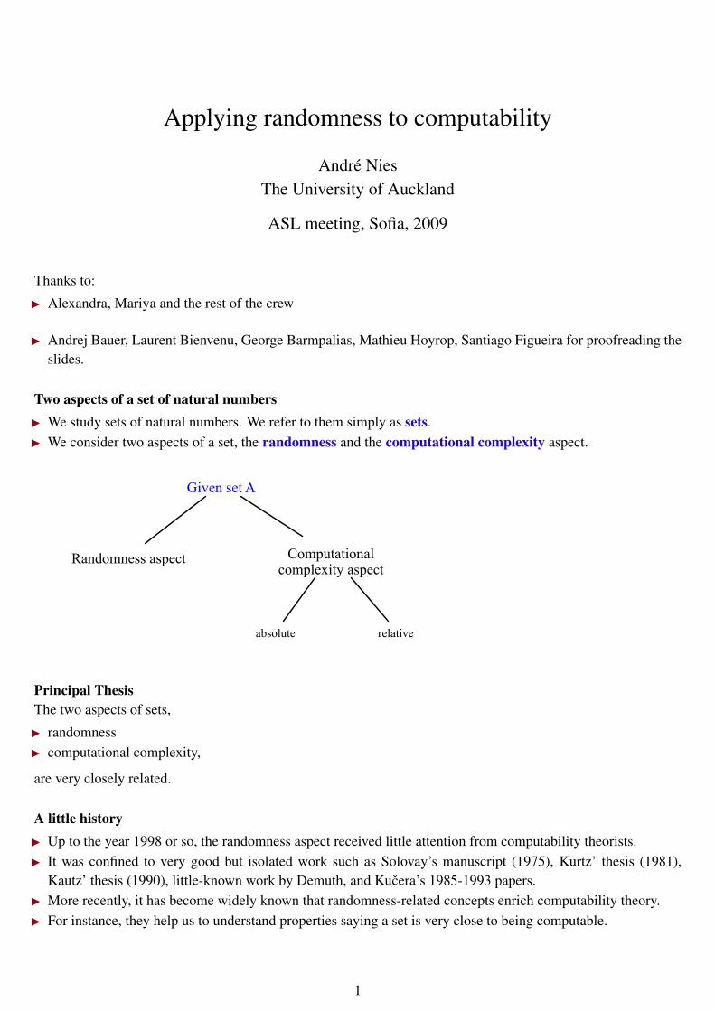
Two aspects of a set of natural numbersI We study sets of natural numbers. We refer to them simply as sets.I We consider two aspects of a set, the randomness and the computational complexity aspect.
Given set A
Randomness aspect Computational complexity aspect
absolute relative
Principal ThesisThe two aspects of sets,
I randomnessI computational complexity,
are very closely related.
A little historyI Up to the year 1998 or so, the randomness aspect received little attention from computability theorists.I It was confined to very good but isolated work such as Solovay’s manuscript (1975), Kurtz’ thesis (1981),
Kautz’ thesis (1990), little-known work by Demuth, and Kucera’s 1985-1993 papers.I More recently, it has become widely known that randomness-related concepts enrich computability theory.I For instance, they help us to understand properties saying a set is very close to being computable.
1
Important work 1999-2003I ‘Lowness for the class of random sets” (1999) by Kucera and Terwijn;
I “R.e. reals and Chaitin Omega numbers” by Calude, Hertling, Khoussainov, Wang (2001); subsequent paper“Randomness and recursive enumerability” by Kucera and Slaman (2001);
I “Trivial reals” by Downey, Hirschfeldt, Nies, Stephan (2003).
I “Lowness properties and randomness” by Nies (published 2005).
The plan for Lecture 1We provide background.
I We review some important concepts from computability. We clarify the computational complexity aspect of aset.
I We define descriptive complexity of strings x, introducing the complexity measure K(x).
Also today, we consider the classical interaction,from computability to randomness.
I We use algorithmic tools to introduce a hierarchy of mathematical randomness notions.I We study these notions, again with algorithmic tools.
The interaction from randomness to computabilityI In the Lectures 2 and 3, we apply randomness to understand the computational complexity of sets.
I More generally, we show how randomness-related concepts enrich computability theory.
Lecture 3 also covers some connections to effective descriptive set theory.
Some referencesCalibrating randomness by Downey, Hirschfeldt, N, Terwijn. BSL 12 (2006), 411-491.
!"#$%&'#()*+,$-#'.##&$/01)2'+-%*%',$+&3$(+&301,$"+4$-##&$
+&$+/'%5#$+(#+$06$(#4#+(/"$%&$(#/#&'$,#+(47$(#6*#/'#3$-,$+1)*#$62&3%&8$%&$
'"#$9:;7$&21#(024$.0(<4"0)47$+&3$)2-*%/+'%0&4$0&$'"#$42-=#/'>$!"#$
/01)*#?%',$+&3$'"#$(+&301,$+4)#/'$06$+$4#'$06$&+'2(+*$&21-#(4$+(#$
/*04#*,$(#*+'#3>$!(+3%'%0&+**,7$/01)2'+-%*%',$'"#0(,$%4$/0&/#($.%'"$'"#$
/01)*#?%',$+4)#/'>$@0.#5#(7$/01)2'+-%*%',$'"#0(#'%/$'00*4$/+&$+*40$-#$
24#3$'0$%&'(032/#$1+'"#1+'%/+*$/02&'#()+('4$60($'"#$%&'2%'%5#$&0'%0&$06$
(+&301,$06$+$4#'>$A#/#&'$(#4#+(/"$4"0.4$'"+'7$/0&5#(4#*,7$/0&/#)'4$
+&3$1#'"034$0(%8%&+'%&8$6(01$(+&301,$#&(%/"$/01)2'+-%*%',$'"#0(,>$
$
B05#(%&8$'"#$-+4%/4$+4$.#**$+4$(#/#&'$(#4#+(/"$(#42*'47$'"%4$-00<$
)(05%3#4$+$5#(,$(#+3+-*#$%&'(032/'%0&$'0$'"#$#?/%'%&8$%&'#(6+/#$06$
/01)2'+-%*%',$+&3$(+&301,$60($8(+32+'#4$+&3$(#4#+(/"#(4$%&$
/01)2'+-%*%',$'"#0(,7$'"#0(#'%/+*$/01)2'#($4/%#&/#7$+&3$1#+42(#$'"#0(,>$
$
!"#$%#$&'((C(#6+/#$$
D>$!"#$/01)*#?%',$06$4#'4$
E>$!"#$3#4/(%)'%5#$/01)*#?%',$06$4'(%&84$
F>$G+('%&H$IJ6$(+&301,$+&3$%'4$5+(%+&'4$
K>$L%+80&+**,$&0&/01)2'+-*#$62&/'%0&4$
M>$I0.,$C(0)#('%#4$+&3$!H'(%5%+*%',$
N>$:01#$+35+&/#3$/01)2'+-%*%',$'"#0(,$
O>$A+&301,$+&3$-#''%&8$4'(+'#8%#4$
P>$B*+44#4$06$/01)2'+'%0&+*$/01)*#?%',$
Q>$@%8"#($/01)2'+-%*%',$+&3$(+&301,$
!"##$%&'!"#$%&'%!#()*+,-!
.&/%000000000000000000000000000000000000000000000000000000000000000!
1*'+)+2+)3*000000000000000000000000000000000000000000000000000000000000!
455(%''00000000000000000000000000000000000000000000000000000000000000!
6)+7000000000000000000000000! !!!!!!!!!!!!!!!!!!!!8+&+%00000000!!!!!!!!!!!!9)#000000000000!
:&7+)/%!;<3*%00000000000000000000000000000!$
()"*$%&'!")=!5)==%(%*+!=(3/!&>3?%-!
.&/%000000000000000000000000000000000000000000000000000000000000000!
1*'+)+2+)3*000000000000000000000000000000000000000000000000000000000000!
455(%''00000000000000000000000000000000000000000000000000000000000000!
6)+7000000000000000000!000000000000000000!!8+&+%0000000!!9)#0000000000000!
!
!"#!"#!"#!"#$%&'($')%'&*$%&'($')%'&*$%&'($')%'&*$%&'($')%'&*$$$$
;$%&'%!(%+2(*!+<)'!=3(/@!&$3*A!B)+<!732(!C(%5)+!C&(5!)*=3(/&+)3*@!+3,!!DE=3(5!F*)?%(')+7!;(%''@!D(5%(!:%#+G@!HIIJ!K?&*'!L3&5@!6&(7@!.6!HMNJO!
;$%&'%!'%*5!/%,! ! ! ! ! ! !
0000!C3#)%'!3=!63/#2+&>)$)+7!&*5!L&*53/*%''!!!!!!!!!!!!PMQRIRJPRPHOIMSRJ!!!!TJJIGII!U+,,-..$
;$%&'%!)*C$25%!TNGNI!'<)##)*A!&*5!<&*5$)*A!=3(!+<%!=)('+!>33V@!TJGNI!=3(!%&C<!&55)+)3*&$!>33VG!"W4@!W1@!64@!X!.6!(%')5%*+'!#$%&'%!&55!'&$%'!+&EG-!$
*/0123%$"34&51/%"&3'$
$K*C$3'%5!)'!&!C<%CV!3(!/3*%7!3(5%(!/&5%!32+!+3!DE=3(5!F*)?%(')+7!;(%''!=3(!T0000$
!;$%&'%!C<&(A%!/7!C(%5)+!C&(5,$
!!!!!!!!!!! !Y184!!! !Z&'+%(!6&(5!!!! !4/%()C&*!KE#(%''!
6(%5)+!6&(5!*3G0000000000000000000000000000000000000000!!KE#G!:&+%000000000!
8)A*&+2(%00000000000000000000000000000000000000000000000000000000000000!!"#$%&'%!()*%+!,-%./*!0&-.!)-.%-'!&-%!1)*!2&$/.!3/*4)5*!&!'/61&*5-%!&1.!7/$$/16!&..-%''8!9%!'5-%!*)!0):;$%*%!*4%!7/$$/16!/1<)-:&*/)1!'%0*/)1=!4$$!'&$%'!'2>[%C+!+3!&CC%#+&*C%!>7!DE=3(5!F*)?%(')+7!;(%''!&+!)+'!3==)C%'!)*!6&(7@!.6G!D==%(!Y&$)5!)*!+<%!FG8G!3*$7G!!
BRGC9!;STIT!U$;VL$A;VLRGVW::$
;&3(X$V%#4$
EYYQ$$KEY$))>$
DF$*%&#$%**24>$$
QOPHYHDQHQEFYONHD$
ZDDY>YY$)**+,,$
-./%(((((0,1(
&5625$4&517$(/82$9.:$
B+**(2+*,,+342+5446([GH\7$PHM]FY$W:!^$0($6+?$2+727+655+28,8$$R(3#($0&*%&#$+'(999+":;+<"=>:&(+&3$#&'#($)(010'%0&$/03#(0637,((
'0(&./%(0,1$
Y)')+!2'!&+!BBBG32#GC3/U2'!+3!'%%!32(!3+<%(!%EC)+)*A!+)+$%'\!
My book “Computability and Randomness”,Oxford University Press, 447pp, Feb. 2009.
Forthcoming book “Algorithmic randomness and complexity” by Downey and Hirschfeldt.
These slides.
Further material:Recent talk “New directions in computability and randomness” (open questions); recent workshop tutorials“Cost functions”, “Randomness via effective descriptive set theory” all on my web site.
2
Part I
Computability and its application to randomness1 Background from computability theory
Contents
Oracle computationsI All concepts in computability are ultimately based on (Turing machine) computations.
I Equipping the machine with an oracle X , we get a version of the concept relative to X .
I For instance, “A is computable” becomes “A is computable in X”, written A ≤T X .
Turing functionalsI Let (Me)e∈N be an effective listing of all oracle Turing machines.
Let (Φe)e∈N be the corresponding effective list of Turing functionals.ΦXe is the partial function determined by Me with oracle X .
I Thus, A ≤T X ⇐⇒ ∃e [A = ΦXe ]. (Here we identify the set A ⊆ N with its characteristic function N →
0, 1.)
I A ≤tt X if in addition, the running time is computably bounded in the input. (This is called truth-tablereducibility because the oracle computations can be viewed as evaluating an effectively determined Booleanfunction on the answers to oracle queries.)
The Turing jumpI JX(e) is a universal Turing functional.
For instance, let JX(e) ' ΦXe (e).
I X ′ = e : JX(e) is defined is the halting problem relative to X .
I X ′ is computably enumerable relative to X , and X ′ >T X .
I ∅′ is the usual halting problem.
I A ≤T B implies A′ ≤T B′.
I A is ∆02⇐⇒ A ≤T ∅′.
The Shoenfield Limit LemmaI A is ∆0
2 ⇐⇒ A(x) = lims f(x, s) for some computable 0, 1-valued function f . Often, we don’t name suchan approximating function explicitly, and rather write As(x) instead of f(x, s).
I A ≤tt ∅′ if in addition, the number of changes in some computable approximation is computably bounded in x.(Such a set is called ω-c.e.)
3
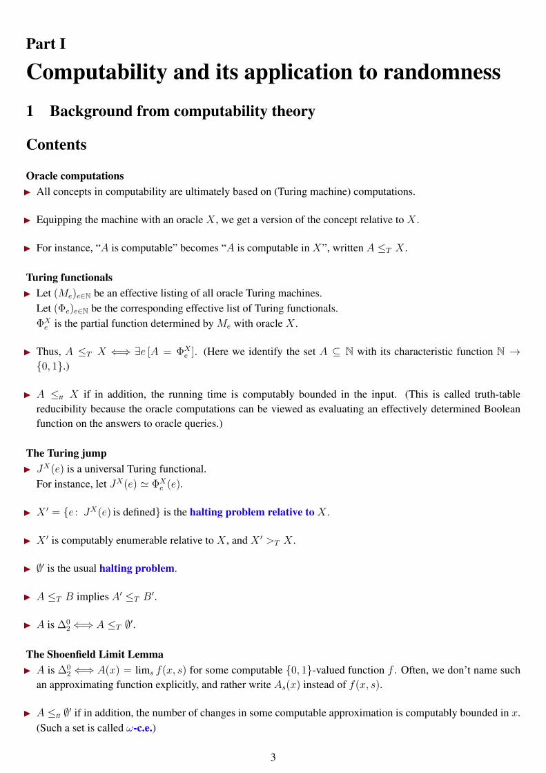
Lowness properties and highness propertiesI A lowness property specifies a sense in which a set is close to computable. It is closed downwards under≤T .I A highness property specifies a sense in which a set almost computes ∅′. It is closed upwards under ≤T .
Example 1. A ⊆ N is low if A′ ≤T ∅′, and A is high if ∅′′ ≤T A′.
∅'High sets
computable sets Low sets
Lowness, highness, dominationBy the Limit Lemma, A′ ≤T ∅′ ⇐⇒ there is a computable 0,1-valued approximation f(x, s) to the questionwhether x ∈ A′. That is,
A′(x) = limsf(x, s).
Highness ∅′′ ≤T A′ can be characterized via domination.
Theorem 2 (Martin 1966). A is high ⇐⇒ some function f ≤T A dominates each computable function (onalmost all arguments).
A set can be complex in one sense, and computationally weak in another sense. For instance, there is a high setof minimal Turing degree (Cooper).
ConventionsI x, y, z, σ, τ denote strings from 0, 1∗.
I We can identify strings with numbers via a computable bijection 0, 1∗ ↔ N (related to the binary presenta-tion).
I The capital letters A,B,C,X, Y, Z denote sets of natural numbers.
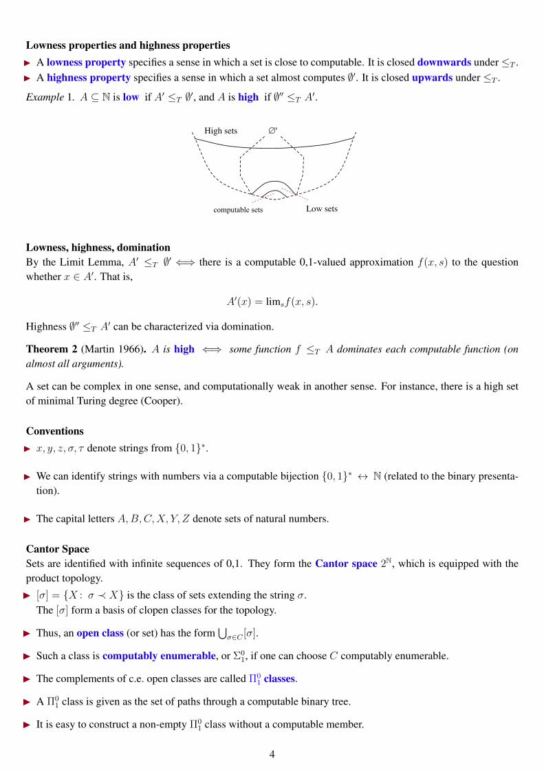
Cantor SpaceSets are identified with infinite sequences of 0,1. They form the Cantor space 2N, which is equipped with theproduct topology.
I [σ] = X : σ ≺ X is the class of sets extending the string σ.The [σ] form a basis of clopen classes for the topology.
I Thus, an open class (or set) has the form⋃σ∈C [σ].
I Such a class is computably enumerable, or Σ01, if one can choose C computably enumerable.
I The complements of c.e. open classes are called Π01 classes.
I A Π01 class is given as the set of paths through a computable binary tree.
I It is easy to construct a non-empty Π01 class without a computable member.
4
Basis Theorems for Π01 classes
Definition 3. A is computably dominated ⇐⇒ each function f ≤T A is dominated by a computable function.
This lowness property is incompatible with being low in the usual sense. In fact, the only computably dominated∆0
2 sets are the computable sets.A basis theorem (for Π0
1 classes) says that each non-empty Π01 class has a member with a particular property
(often, a lowness property).
Theorem 4 (Jockusch and Soare 1972). Let P be a non-empty Π01 class.
• P has a low member.
• P has a computably dominated member.
2 Descriptive string complexity
Contents
Prefix free machinesI Let 0, 1∗ be the strings over 0, 1. A machine is a partial recursive function M : 0, 1∗ 7→ 0, 1∗.
I If M(σ) = x we say that σ is an M -description of x.
I We say that M is prefix free if no M -description is a proper initial segment of any other M -description.
The universal prefix free machine, and K(x)
I Let (Md)d∈N be an effective listing of all prefix free machines. We define a universal prefix free machine U by
U(0d1σ) 'Md(σ).
I Given string x, the prefix free descriptive string complexity K(x) is the length of a shortest U-description ofx:
K(x) = min|σ| : U(σ) = x.
Some facts about KLet “≤+ denote “≤” up to a constant. (For instance, 2n+ 5 ≤+ n2.)Let |x| ∈ 0, 1∗ denote the length of a string x, written in binary.The following bounds are proved by constructing appropriate prefix free machines.I For each computable function f we have
K(f(x)) ≤+ K(x).
In particular, we have the lower bound K(|x|) ≤+ K(x).I We have the upper bound
K(x) ≤+ |x|+K(|x|).
I Also K(|x|) ≤+ 2 log |x|, so the upper bound is not far beyond |x|.I IfK(x) ≥+ |x|we think of x as incompressible. This formalizes the intuitive notion of randomness for strings.
5
Quiz 1
(1) Can a high set be computably dominated?
(2) Is “not low”, i.e A′ 6≤T ∅′, a highness property?
(3) Define a prefix free machine showing that K(x) ≤+ |x|+K(|x|).
3 Randomness for infinite objects
Contents
Degree of randomness for sequences of bits
Sequences of bits - are they random?
000000000000000000000000000000000000. . .
101001000100001000001000000100000001. . .
001001000011111101101010100010001000. . .
100101000001000111110100001011011111. . .
111011010111101010101111110011101110. . .
Explanations:
Only zeros
each time one more zero in between the ones
π − 3 in binary
Coin tossing
Coin tossing
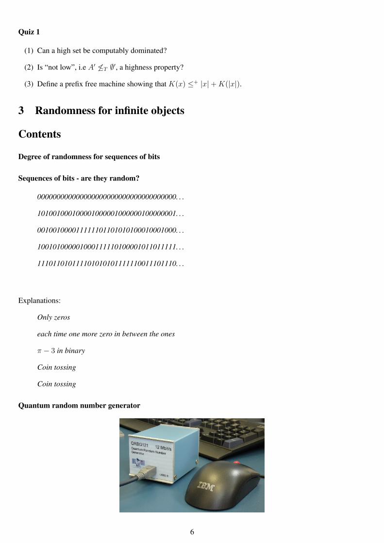
Quantum random number generator
6
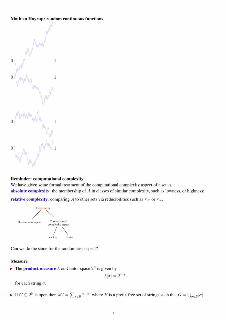
Mathieu Hoyrup: random continuous functions
0 1
0 1
0 1
0 1
Reminder: computational complexityWe have given some formal treatment of the computational complexity aspect of a set A.absolute complexity: the membership of A in classes of similar complexity, such as lowness, or highness;
relative complexity: comparing A to other sets via reducibilities such as ≤T or ≤tt.
Given set A
Randomness aspect Computational complexity aspect
absolute relative
Can we do the same for the randomness aspect?
MeasureI The product measure λ on Cantor space 2N is given by
λ[σ] = 2−|σ|
for each string σ.
I If G ⊆ 2N is open then λG =∑
σ∈B 2−|σ| where B is a prefix free set of strings such that G =⋃σ∈B[σ].
7
I C ⊆ 2N is null if C is contained in some Borel B such that λB = 0.
Null classes and randomnessThe intuition: an object is random if it satisfies no exceptional properties.Here are some examples of exceptional properties of a set Y :I Having every other bit zero:
∀i Y (2i) = 0.
I Having at least twice as many zeros as ones in the limit:
2/3 ≤ lim inf |i < n : Y (i) = 0|/n.
We would like to formalize “exceptional property” by “null class”.
• The examples above are null classes, so they should not contain a random set.
• The problem: if we do this, no set Z is random, because Z itself is a null class!
The solution: effective null classesI Using algorithmic tools, we introduce effective null classes, also called tests.
I To be random in an algorithmic sense, Z merely has to avoid these effective null classes, that is, pass thosetests.
Tests
Fact 5. The class C ⊆ 2N is null ⇐⇒ C ⊆⋂Gm for some sequence (Gm)m∈N of open sets such that λGm → 0.
We obtain a type of effective null class (or test) by adding effectivity restrictions to this condition characterizingnull classes.
(1) Require an effective presentation of (Gm)m∈N;
(2) possibly, require fast convergence of λGm → 0.
By (1) there are only countably many effective null classes. Their union is still a null class and contains allnon-random sets in this sense. So each effective randomness notion has measure 1.
Martin-Löf’s randomness notion (1966)
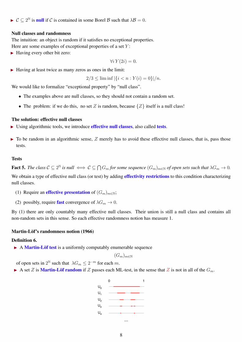
Definition 6.I A Martin-Löf test is a uniformly computably enumerable sequence
(Gm)m∈N
of open sets in 2N such that λGm ≤ 2−m for each m.I A set Z is Martin-Löf random if Z passes each ML-test, in the sense that Z is not in all of the Gm.
0 1
...
U0U1U2U3U4
8
Chaitin’s halting probabilityWe identify coinfinite sets with real numbers in [0, 1).I Consider the halting probability of the universal prefix free machine U,
Ω =∑
U(σ) halts
2−|σ|.
I Note that this sum converges because U is prefix free.I Ω is Martin-Löf random (Chaitin).I The left cut q ∈ Q : q < Ω is computably enumerable.I Ω ≡T ∅′.
Characterization via the initial segment complexityGiven Z and n ∈ N, let Z n denote the initial segment Z(0) . . . Z(n− 1).
Schnorr’s Theorem says that Z is ML-random ⇐⇒ each initial segment of Z is incompressible.Let K(x) be the length of a shortest prefix free description of string x.
Theorem 7 (Schnorr 1973). Z is ML-random ⇐⇒ there is b ∈ N such that ∀nK(Z n) > n− b.
Levin (1973) proved the analogous theorem for monotone string complexity.
A universal Martin-Löf testSchnorr’s Theorem yields a universal ML-test:I LetRb = X : ∃n [K(X n) ≤ n− b].
I Rb is uniformly c.e. open, because the relation “K(x) ≤ r” is Σ01.
I One shows that λRb ≤ 2−b.
I With this notation, Schnorr’s Theorem says thatZ is ML-random ⇐⇒ Z passes the test (Rb)b∈N.
I So, the single test (Rb)b∈N is enough!
ML-random sets with lowness propertiesI Consider the complement ofR1:
X : ∀nK(X n) ≥ n− 1.
This is a Π01 class of measure ≥ 1/2.
I By Schnorr’s Theorem, it consists entirely of ML-random sets.I So we can apply the Jockusch-Soare basis theorems to obtain random sets with lowness properties:
Example 8.
• There is a low ML-random set.
• There is a computably dominated ML-random set.
9
Schnorr randomnessSchnorr criticized that Martin-Löf-randomness is too strong to be considered algorithmic. He proposed a re-stricted test notion where we know more about the tests.I A Schnorr test is a ML-test (Gm)m∈N such that λGm is a computable real uniformly in m.I Z is Schnorr random if Z 6∈
⋂mGm for each Schnorr test (Gm)m∈N.
It suffices to consider the tests (Gm)m∈N where λGm = 2−m.
Schnorr randoms in each high degree
Theorem 9 (Nies, Stephan, Terwijn, 2005; Downey, Griffiths, 2005). For each high set A there is a Schnorrrandom set Z ≡T A.
I Schnorr random sets satisfy all statistical criteria for randomness, such as the law of large numbers.I They do not satisfy all computability-theoretic criteria.I For instance, there is a high minimal Turing degree, hence a Schnorr random set Z of minimal degree.
• If Z0 is the bits in even position, and Z1 the bits in odd position, then both Z0, Z1 are incomputable.
• Hence Z0 ≡T Z1.
• Note that such a set Z is not ML-random.
Theory of Schnorr randomnessI The theory of Schnorr randomness parallels the theory of ML-randomness.
I This is surprising because there is no universal Schnorr test.
I The actual results are quite different.
Characterization via the initial segment complexityA prefix free machineM is called computable measure machine if its halting probability ΩM =
∑M(σ) halts 2−|σ|
is a computable real number. For instance, define M by M(0n1) = n in binary. Then ΩM = 1.I Recall Z is Martin-Löf random ⇐⇒ for some b, ∀n K(Z n) > n− b.I The following is an analog for Schnorr randomness. Since there is no universal computable measure machine,
we have to quantify over all of them.I For a prefix free machine M ,
KM(x) = length of a shortest M -description of x.
Theorem 10 (Downey, Griffiths, 2005). Z is Schnorr random ⇐⇒ for each computable measure machine M ,for some b, ∀n KM(Z n) > n− b.
Weak 2-randomnessOne can argue that ML-randomness is too weak.For instance, the ML-random real Ω has a computably enumerable left cut, and computes the halting problem.These properties may contradict our intuition of randomness.Recall: a ML-test is a uniformly computably enumerable sequence (Gm)m∈N of open sets such that λGm ≤ 2−m
for each m.I If the condition “λGm ≤ 2−m for each m” is removed (and we only retain the basic condition limmλGm = 0),
we obtain a test concept equivalent to null Π02 classes.
I We say that Z is weakly 2-random if Z is in no null Π02 class.
If Z is ∆02 then Z is a Π0
2 class. Thus, no ∆02 set is weakly 2-random. This rules out Ω as weakly 2-random.
10
2-randomnessFinally, Z is called 2-random if Z is ML-random relative to ∅′.We have the proper implications
2-random ⇒ weakly 2-random ⇒ Martin-Löf ⇒ Schnorr.
2-randomness can be characterized by strong incompressibility of infinitely many initial segments.Let C(x) denote the plain Kolmogorov complexity of a string x. Note that C(x) ≤+ |x|.
Theorem 11. Z is 2-random⇐⇒ C(Z n) =+ n for infinitely many n (N,S,T, 2005; Miller, 2005)⇐⇒ K(Z n) =+ n+K(n) for infinitely many n (Miller, 2008).
No initial segment characterization is known for weak 2-randomness.
4 Studying randomness notions via computability
Contents
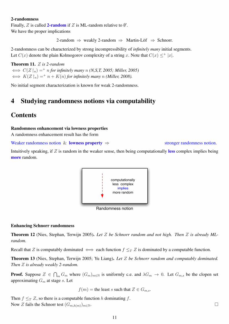
Randomness enhancement via lowness propertiesA randomness enhancement result has the form
Weaker randomness notion & lowness property ⇒ stronger randomness notion.
Intuitively speaking, if Z is random in the weaker sense, then being computationally less complex implies beingmore random.
Randomness notion
computationally less complex
impliesmore random
Enhancing Schnorr randomness
Theorem 12 (Nies, Stephan, Terwijn 2005). Let Z be Schnorr random and not high. Then Z is already ML-random.
Recall that Z is computably dominated ⇐⇒ each function f ≤T Z is dominated by a computable function.
Theorem 13 (Nies, Stephan, Terwijn 2005; Yu Liang). Let Z be Schnorr random and computably dominated.Then Z is already weakly 2-random.
Proof. Suppose Z ∈⋂mGm where (Gm)m∈N is uniformly c.e. and λGm → 0. Let Gm,s be the clopen set
approximating Gm at stage s. Let
f(m) = the least s such that Z ∈ Gm,s.
Then f ≤T Z, so there is a computable function h dominating f .Now Z fails the Schnorr test (Gm,h(m))m∈N.
11
Enhancing Martin-Löf randomnessHere, the randomness notion stronger than ML-randomness actually implies the lowness property. So we havecharacterization :Martin-Löf randomness =⇒
lowness property ⇐⇒ stronger randomness notion.
Theorem 14 (Hirschfeldt, Miller 2006). Let Z be ML-random. Then: every ∆02 set Turing below Z is computable
⇐⇒ Z is weakly 2-random
“⇐” extends the fact that a weakly 2-random is not ∆02.
“⇒” relies on the cost function method of Lecture 2.
We say that Z is low for Ω if Chaitin’s Ω is ML-random relative to Z.
Theorem 15 (Nies, Stephan, Terwijn 2005). Let Z be ML-random. ThenZ is low for Ω ⇐⇒ Z is 2-random.
This uses a theorem of van Lambalgen on relative ML-randomness.
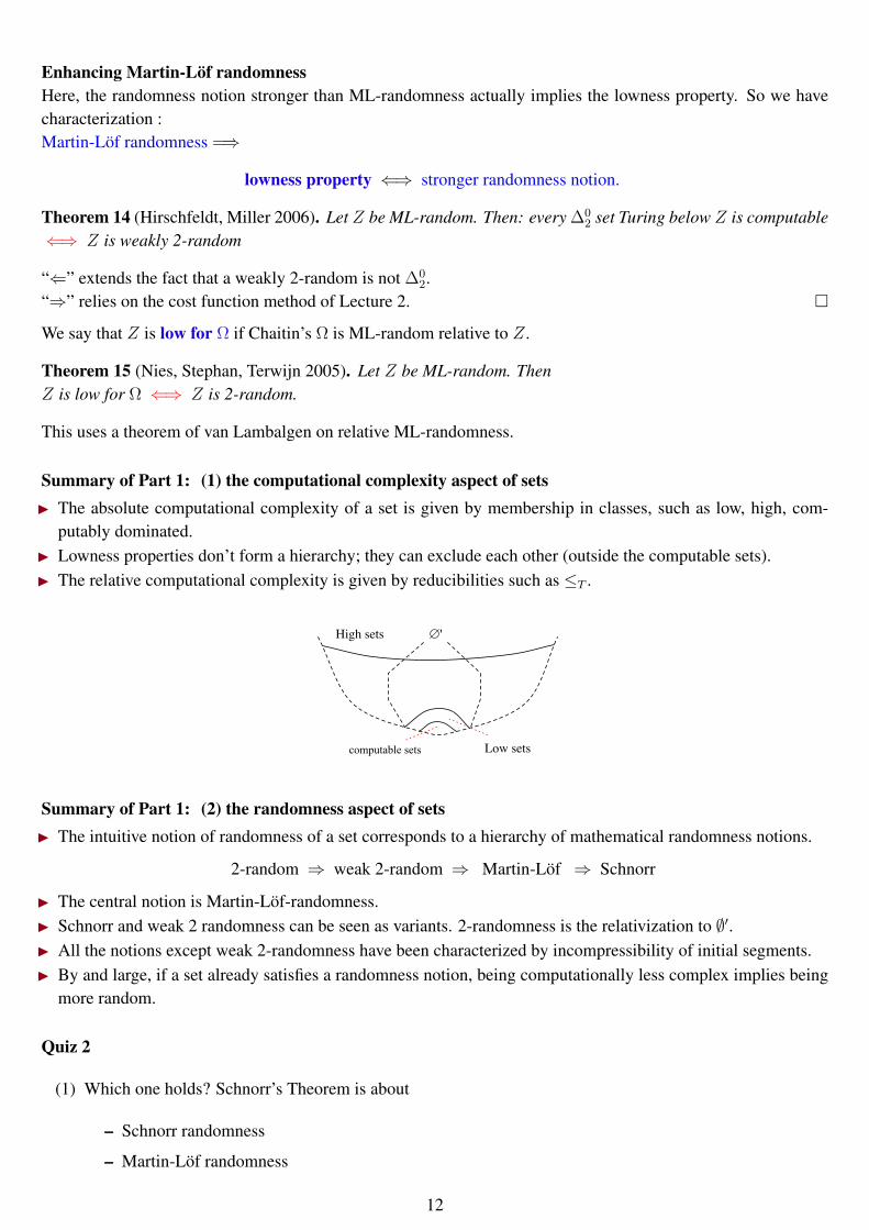
Summary of Part 1: (1) the computational complexity aspect of setsI The absolute computational complexity of a set is given by membership in classes, such as low, high, com-
putably dominated.I Lowness properties don’t form a hierarchy; they can exclude each other (outside the computable sets).I The relative computational complexity is given by reducibilities such as ≤T .
∅'High sets
computable sets Low sets
Summary of Part 1: (2) the randomness aspect of setsI The intuitive notion of randomness of a set corresponds to a hierarchy of mathematical randomness notions.
2-random ⇒ weak 2-random ⇒ Martin-Löf ⇒ Schnorr
I The central notion is Martin-Löf-randomness.I Schnorr and weak 2 randomness can be seen as variants. 2-randomness is the relativization to ∅′.I All the notions except weak 2-randomness have been characterized by incompressibility of initial segments.I By and large, if a set already satisfies a randomness notion, being computationally less complex implies being
more random.
Quiz 2
(1) Which one holds? Schnorr’s Theorem is about
– Schnorr randomness
– Martin-Löf randomness
12
– cats.
(2) Give an example of a 2-random set. Give examples showing that the implications are proper:
2-random ⇒ weak 2-random ⇒ Martin-Löf ⇒ Schnorr.
Note here that no 2-random set is computably dominated (Kurtz, 1981).
(3) Suppose A is computable. If Z satisfies a randomness notion, show that Z∆A satisfies the same notion.
Part II
Lowness properties within the ∆02 sets
The plan for Part 2I We introduce lowness properties within the ∆0
2 sets.
I We investigate them using randomness notions.
I We introduce the K-trivial sets which are far from random.
I The cost function method is used to build ∆02 sets with lowness properties.
Lowness paradigmsA lowness property specifies a sense in which a set is close to computable. There are several paradigms:
1. Weak as an oracle.Examples: lowness A′ ≤T ∅′; being computably dominated (each function f ≤T A is dominated by a com-putable function).
2. Easy to compute. The class of oracles computing A is large in some sense.We’ll see examples shortly, such as sets computed by random oracles.
3. For a ∆02 set: Inertness, i.e. computably approximable with a small total of mind changes
5 Subclasses of the low sets, and the amount of injury
Contents
How low is the property A′ ≤T ∅′?
Definition 16. The coinfinite computably enumerable set A is called simple if it has a non-empty intersectionwith each infinite c.e. set.
Such a set is incomputable as its complement is not c.e.
Some existence results for low sets:
(1) The Low Basis Theorem (Jockusch and Soare 1972).
13
(2) There is a low simple set (1957). This provides a solution to Post’s 1944 problem whether some c.e. set isneither computable nor Turing complete.
(3) There are disjoint low c.e. sets A0, A1 such that ∅′ = A0 ∪ A1. (Sacks Splitting Theorem,1962.)
By (3), lowness does not necessarily mean very close to computable.
Superlowness
Definition 17 (Bickford and Mills 1982; Mohrherr 1986). A is called superlow if A′ ≤tt ∅′. That is, one canapproximate A′(x) with a computably bounded number of mind changes.
Recall the existence results for lowness:
(1) Low Basis Theorem.
(2) There is a low simple set.
(3) There are disjoint low c.e. sets A0, A1 such that ∅′ = A0 ∪ A1.
I The proofs of (1) and (2) actually yield superlowness.I In contrast, (3) fails for superlowness.
Building a low simple set ATo make A simple we meet the simplicity requirements
Se : |We| =∞⇒ A ∩We 6= ∅.
To make A low, we meet the lowness requirements
Li : JA(i) is defined at infinitely many stages⇒ JA(i) converges.
Let We[s] be the finite set of numbers that have entered We by stage s.
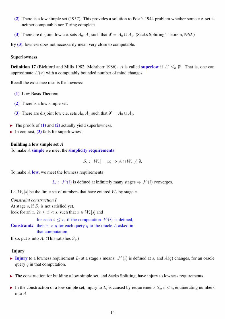
Constraint construction IAt stage s, if Se is not satisfied yet,look for an x, 2e ≤ x < s, such that x ∈ We[s] and
Constraint:for each i ≤ e, if the computation JA(i) is defined,then x > q for each query q to the oracle A asked inthat computation.
If so, put x into A. (This satisfies Se.)
InjuryI Injury to a lowness requirement Li at a stage s means: JA(i) is defined at s, and A(q) changes, for an oracle
query q in that computation.
I The construction for building a low simple set, and Sacks Splitting, have injury to lowness requirements.
I In the construction of a low simple set, injury to Li is caused by requirements Se, e < i, enumerating numbersinto A.
14
The amount of injuryI To show lowness, at stage s we guess that
i ∈ A′ if JA(i) is defined at this stage.
I The priority ordering of requirements is L0, S0, L1, S1, . . ..I Since Se acts at most once, Li can be injured at most i times. Hence the guess goes wrong at most i times, andA is in fact superlow.
I In Sacks Splitting, the number of injuries to lowness requirements is not computably bounded. In fact we knowthat the sets cannot both be superlow.
I Our intuition: when we build a c.e. set, the less injury we have, the closer to computable will the set be. Thenext theorem gives further evidence for this principle:
I we use ML-randomness to provide a solution to Post’s problem without injury. We will see later on that theresulting set A is much closer to being computable than the previous examples.
Kucera’s 1985 Theorem (in fact, a special case)
Theorem 18. Let Y be ∆02 and ML-random. Then there is a simple set A ≤T Y .
Now let Y be the bits of Ω in the even positions. Then an easy direct proof shows that Y is low and ML-random(N,S, T 2005). Therefore:
Corollary 1. We can build without injury a low simple set A.
Proof of the theorem: A Solovay test G is given by an effective enumeration of strings σ0, σ1, . . ., such that∑i 2−|σi| <∞.
If Y is ML-random, then for almost all i, σi 6 Y .
Proof of Kucera’s theoremAs before, we meet the simplicity requirements
Se : |We| =∞⇒ A ∩We 6= ∅.
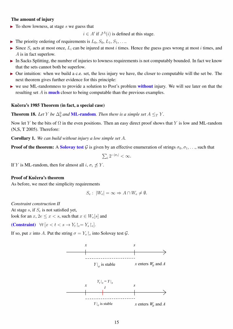
Constraint construction IIAt stage s, if Se is not satisfied yet,look for an x, 2e ≤ x < s, such that x ∈ We[s] and
(Constraint) ∀t [x < t < s→ Yt e= Ys e].
If so, put x into A. Put the string σ = Ys e into Solovay test G.
x
x enters W and AeY |e is stable
s
x
x enters W and AeY |e is stable
stYt |x = Y |x
15
• Each Se is met, so A is simple.
• G is a Solovay test, as its total is at most∑
e 2−e.
• To see that A ≤T Y , choose s0 such that σ 6 Y for any σ enumerated into G after stage s0.
• Given an input x ≥ s0, using Y as an oracle, compute t > x such that Yt x= Y x. Then x ∈ A ↔ x ∈ At.
• For, if we put x into A at a stage s > t for the sake of Se, then x > e, so we list σ in G where σ = Ys e=Y e;
this contradicts the fact that σ 6 Y .
6 Lowness properties via randomness
Contents
K-trivial⇐⇒ low for ML-randomnessRecall: K(x) = length of a shortest prefix free description of string x.
• A set A is K-trivial if each initial segment of A has prefix free complexity no greater than the one of itslength. That is, there is b ∈ N such that, for each n (written in binary),
K(An) ≤ K(n) + b
(Chaitin, 1975).
• A is low for ML-randomness if each ML-random set is already ML-random relative to A (Zambella,1990).
We will see that these two concepts are equivalent.The harder implication is K-trivial⇒ low for ML-randomness.
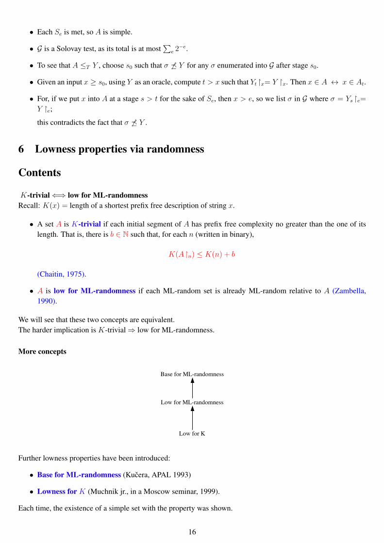
More concepts
Low for K
Low for ML-randomness
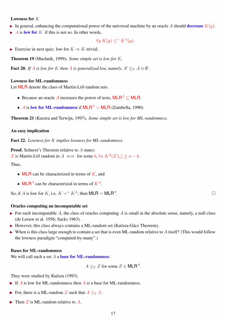
Base for ML-randomness
Further lowness properties have been introduced:
• Base for ML-randomness (Kucera, APAL 1993)
• Lowness for K (Muchnik jr., in a Moscow seminar, 1999).
Each time, the existence of a simple set with the property was shown.
16
Lowness for KI In general, enhancing the computational power of the universal machine by an oracle A should decrease K(y).I A is low for K if this is not so. In other words,
∀y K(y) ≤+ KA(y).
I Exercise in next quiz: low for K ⇒ K-trivial.
Theorem 19 (Muchnik, 1999). Some simple set is low for K.
Fact 20. If A is low for K then A is generalized low, namely, A′ ≤T A⊕ ∅′.
Lowness for ML-randomnessLet MLR denote the class of Martin-Löf-random sets.
• Because an oracle A increases the power of tests, MLRA ⊆ MLR.
• A is low for ML-randomness if MLRA = MLR (Zambella, 1990).
Theorem 21 (Kucera and Terwijn, 1997). Some simple set is low for ML-randomness.
An easy implication
Fact 22. Lowness for K implies lowness for ML-randomness.
Proof. Schnorr’s Theorem relative to A states:Z is Martin-Löf random in A ⇐⇒ for some b, ∀n KA(Z n) ≥ n− b.
Thus,
• MLR can be characterized in terms of K, and
• MLRA can be characterized in terms of KA.
So, if A is low for K, i.e. K =+ KA, then MLR = MLRA.
Oracles computing an incomputable setI For each incomputable A, the class of oracles computing A is small in the absolute sense, namely, a null class
(de Leeuw et al. 1956; Sacks 1963).I However, this class always contains a ML-random set (Kucera-Gács Theorem).I When is this class large enough to contain a set that is even ML-random relative toA itself? (This would follow
the lowness paradigm “computed-by-many”.)
Bases for ML-randomnessWe will call such a set A a base for ML-randomness:
A ≤T Z for some Z ∈ MLRA.
They were studied by Kucera (1993).
I If A is low for ML-randomness then A is a base for ML-randomness.
I For, there is a ML-random Z such that A ≤T Z.
I Then Z is ML-random relative to A.
17
Two theorems
(1) There is a simple base for ML-randomness (Kucera, 1993)
(2) Each base for ML-randomness is low for K. (Hirschfeldt, N, Stephan, 2007)
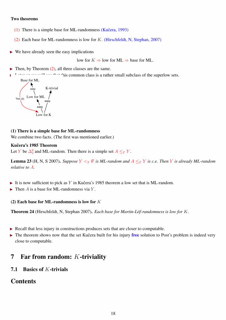
I We have already seen the easy implications
low for K ⇒ low for ML⇒ base for ML.
I Then, by Theorem (2), all three classes are the same.I Later on we will see that this common class is a rather small subclass of the superlow sets.
Low for K
Low for ML
Base for ML
easy
easy
Thm (2)easy
K-trivial
(1) There is a simple base for ML-randomnessWe combine two facts. (The first was mentioned earlier.)
Kucera’s 1985 TheoremLet Y be ∆0
2 and ML-random. Then there is a simple set A ≤T Y .
Lemma 23 (H, N, S 2007). Suppose Y <T ∅′ is ML-random and A ≤T Y is c.e. Then Y is already ML-randomrelative to A.
I It is now sufficient to pick as Y in Kucera’s 1985 theorem a low set that is ML-random.I Then A is a base for ML-randomness via Y .
(2) Each base for ML-randomness is low for K
Theorem 24 (Hirschfeldt, N, Stephan 2007). Each base for Martin-Löf-randomness is low for K.
I Recall that less injury in constructions produces sets that are closer to computable.I The theorem shows now that the set Kucera built for his injury free solution to Post’s problem is indeed very
close to computable.
7 Far from random: K-triviality
7.1 Basics of K-trivials
Contents
18
Intuition on K-trivialityRecall: a set A is K-trivial if, for some b ∈ N
∀n K(An) ≤ K(n) + b,
namely, the K complexity of all the initial segments is minimal.This notion is opposite to ML-randomness:
• Z is ML-random iff all K(Z n) are near the upper bound n+K(n);
• Z is K-trivial if the K(Z n) have the minimal possible value K(n) (all within constants).
Counting theorems of Chaitin, 1976
Counting Theorem for STRINGSFor each b, at most O(2b) strings of length n satisfy K(x) ≤ K(n) + b.
Counting Theorem for SETS(i) For each b, at most O(2b) sets are K-trivial with constant b.(ii) Each K-trivial set is ∆0
2.
For the proof of the second theorem, note thatA is K-trivial via the constant b ⇐⇒
A is a path on the ∆02 tree of strings z such that
K(x) ≤ K(|x|) + b for each x z.
Closure under effective disjoint unionA⊕B is the set which is A on the even bit positions and B on the odd positions.
The counting theorem for strings is used to prove:
Theorem 25 (Downey, H,N , Stephan 2003). IfA andB areK-trivial via b, thenA⊕B isK-trivial via 3b+O(1).
I Idea: it is sufficient to describe each A⊕B 2n with K(n) + 3b+O(1) bits.I We have to describe n only once; if we have a shortest description we also know its length r = K(n);I The set of strings x of length n such that K(x) ≤ r + b has size O(2b);I so, we only need b+O(1) bits each to describe the positions of An and B n in its enumeration.
7.2 Application to Scott classes
Contents
Application to Scott classes
Definition 26. S ⊆ 2N is a Scott class if S is closed downwards under Turing reducibility, closed under joins,and each infinite binary tree T ∈ S has an infinite path in S.
19
Scott classes are the standard systems of models of Peano arithmetic. They also occur in reverse mathematics asthe ω-models of WKL0.
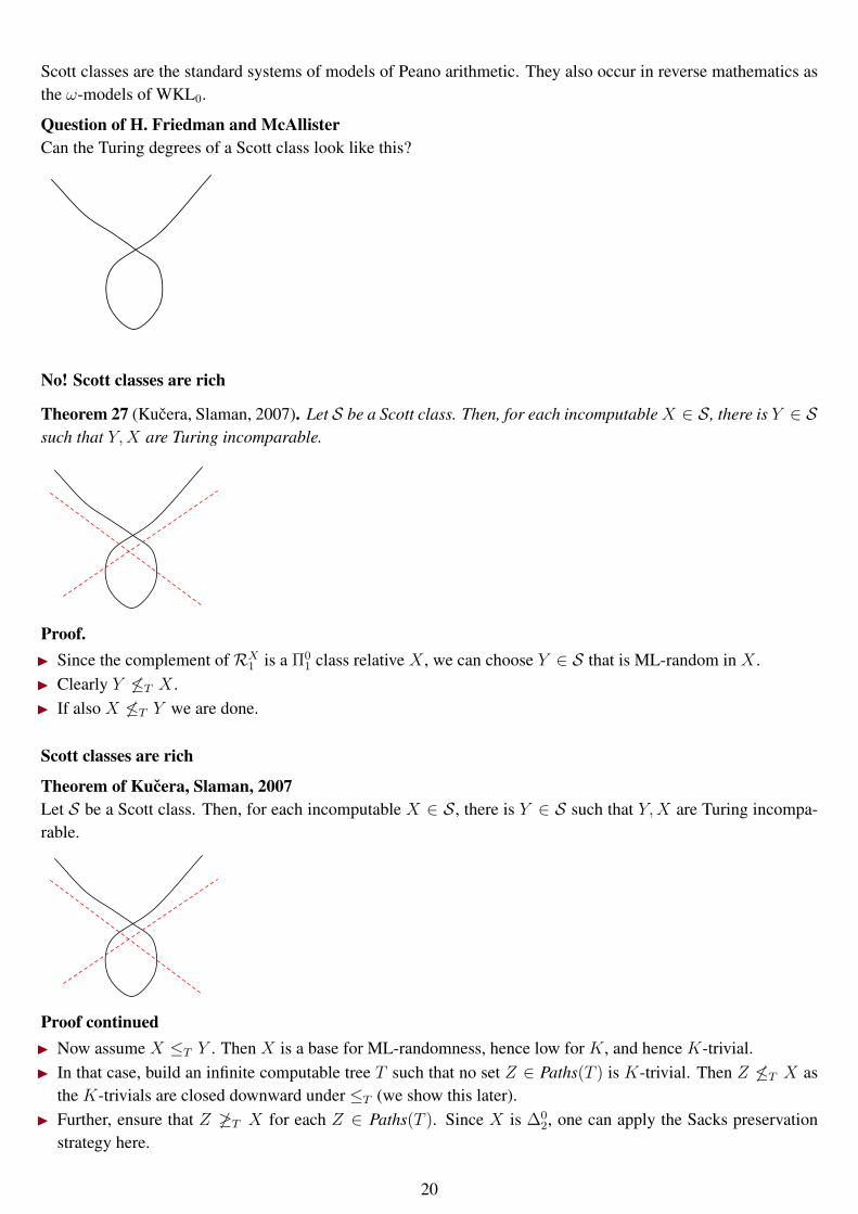
Question of H. Friedman and McAllisterCan the Turing degrees of a Scott class look like this?
No! Scott classes are rich
Theorem 27 (Kucera, Slaman, 2007). Let S be a Scott class. Then, for each incomputableX ∈ S, there is Y ∈ Ssuch that Y,X are Turing incomparable.
Proof.I Since the complement ofRX
1 is a Π01 class relative X , we can choose Y ∈ S that is ML-random in X .
I Clearly Y 6≤T X .I If also X 6≤T Y we are done.
Scott classes are rich
Theorem of Kucera, Slaman, 2007Let S be a Scott class. Then, for each incomputable X ∈ S, there is Y ∈ S such that Y,X are Turing incompa-rable.
Proof continuedI Now assume X ≤T Y . Then X is a base for ML-randomness, hence low for K, and hence K-trivial.I In that case, build an infinite computable tree T such that no set Z ∈ Paths(T ) is K-trivial. Then Z 6≤T X as
the K-trivials are closed downward under ≤T (we show this later).I Further, ensure that Z 6≥T X for each Z ∈ Paths(T ). Since X is ∆0
2, one can apply the Sacks preservationstrategy here.
20
Quiz 3
(1) Why is there a low c.e. set that is not superlow?
(2) Show that each ∆02 set that is low for Ω is already low for ML-randomness.
(3) Verify that each set that is low for K is K-trivial.
(4) Weak truth table reducibility ≤wtt is Turing reducibility with a computable bound on the maximal oraclequery. Show that the K-trivial sets are closed downward under ≤wtt.
(5) How do we define a Scott class consisting only of low sets?
8 Cost functions
Contents
Cost functions: the storyI The constructions of c.e. sets with strong lowness properties looked all very similar: building a set that is low
for ML-randomness, a K-trivial, and even a simple set below a given ∆02 ML-random.
I The cost function method arose to uniformize these constructions.
I Nowadays cost functions are becoming the primary tool to understand the class ofK-trivials and its subclasses.
Definition of cost functions
Definition 28. A cost function is a computable function
c : N× N→ x ∈ Q : x ≥ 0.
I When building a computable approximation of a ∆02 set A, we view c(x, s) as the cost of changing A(x) at
stage s.
I We want to make the total cost of changes, taken over all x, small.
21
Obeying a cost functionRecall the Limit Lemma: A is ∆0
2 iff A(x) = limsAs(x) for some computable approximation (As)s∈N.
Definition 29. The computable approximation (As)s∈N obeys a cost function c if
∞ >∑
x,s c(x, s) [[x < s & x is least s.t. As−1(x) 6= As(x)]].
We write A |= c (A obeys c) if some computable approximation of A obeys c.
Usually we use this to construct some auxiliary object of finite “weight”, such as a bounded request set (akaKraft-Chaitin set), or a Solovay test.
Basic existence theoremWe say that a cost function c satisfies the limit condition if
limx supsc(x, s) = 0.
Theorem 30 (Kucera, Terwijn 1999; D,H,N,S 2003; . . .). If a cost function c satisfies the limit condition, thensome simple set A obeys c.
We meet the requreiments Se : |We| =∞⇒ A ∩We 6= ∅.
Constraint constructionAt stage s, if Se is not satisfied yet,look for an x, 2e ≤ x < s, such that x ∈ We,s and
(Constraint) c(x, s) ≤ 2−e.
If so, put x into A.
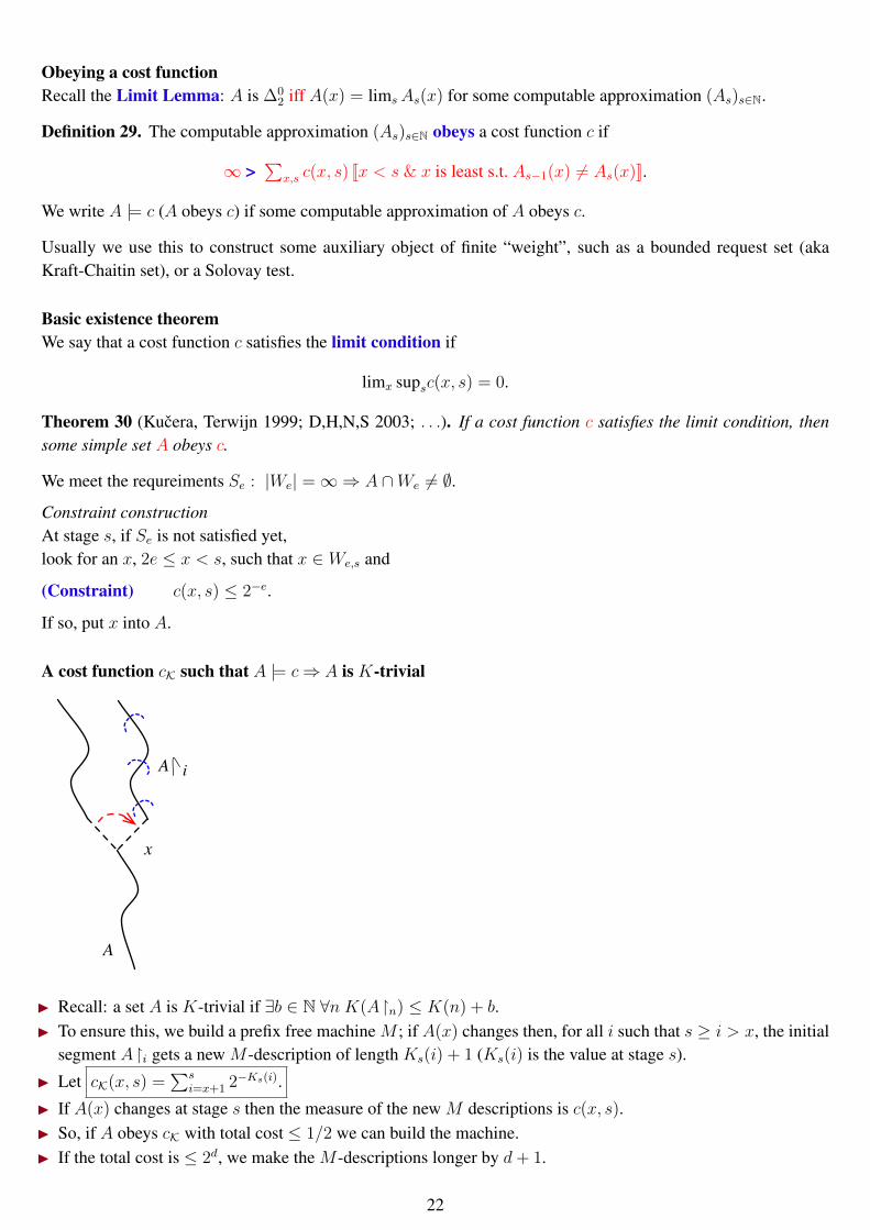
A cost function cK such that A |= c⇒ A is K-trivial
x
A i
A
I Recall: a set A is K-trivial if ∃b ∈ N ∀n K(An) ≤ K(n) + b.I To ensure this, we build a prefix free machine M ; if A(x) changes then, for all i such that s ≥ i > x, the initial
segment Ai gets a new M -description of length Ks(i) + 1 (Ks(i) is the value at stage s).
I Let cK(x, s) =∑s
i=x+1 2−Ks(i).
I If A(x) changes at stage s then the measure of the new M descriptions is c(x, s).I So, if A obeys cK with total cost ≤ 1/2 we can build the machine.I If the total cost is ≤ 2d, we make the M -descriptions longer by d+ 1.
22
Proving Kucera’s Theorem via a cost function
Kucera’s 1986 TheoremSuppose Y is a ML-random ∆0
2 set. Then some simple set A is Turing below Y .
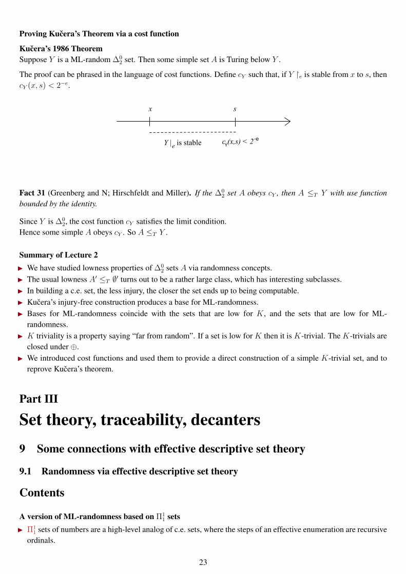
The proof can be phrased in the language of cost functions. Define cY such that, if Y e is stable from x to s, thencY (x, s) < 2−e.
x
Y |e is stable
s
c (x,s) < 2 -eY
Fact 31 (Greenberg and N; Hirschfeldt and Miller). If the ∆02 set A obeys cY , then A ≤T Y with use function
bounded by the identity.
Since Y is ∆02, the cost function cY satisfies the limit condition.
Hence some simple A obeys cY . So A ≤T Y .
Summary of Lecture 2I We have studied lowness properties of ∆0
2 sets A via randomness concepts.I The usual lowness A′ ≤T ∅′ turns out to be a rather large class, which has interesting subclasses.I In building a c.e. set, the less injury, the closer the set ends up to being computable.I Kucera’s injury-free construction produces a base for ML-randomness.I Bases for ML-randomness coincide with the sets that are low for K, and the sets that are low for ML-
randomness.I K triviality is a property saying “far from random”. If a set is low for K then it is K-trivial. The K-trivials are
closed under ⊕.I We introduced cost functions and used them to provide a direct construction of a simple K-trivial set, and to
reprove Kucera’s theorem.
Part III
Set theory, traceability, decanters9 Some connections with effective descriptive set theory
9.1 Randomness via effective descriptive set theory
Contents
A version of ML-randomness based on Π11 sets
I Π11 sets of numbers are a high-level analog of c.e. sets, where the steps of an effective enumeration are recursive
ordinals.
23
I Hyperarithmetical sets are the higher analog of computable sets.
X is hyperarithmetical ⇐⇒both X,N−X are Π1
1 ⇐⇒X ≤T ∅(α) for some computable ordinal α.
Hjorth and Nies (2005) have studied the analogs, based on Π11-sets, of:
string complexity K (written K), and ML-randomness.
• The analog of Schnorr’s Theorem holds. (The proof takes extra effort because of stages that are limitordinals.)
• Some Π11 set of numbers is K-trivial and not hyperarithmetical.
The lowness properties are different now
Theorem 32 (Hjorth and Nies, 2005). If A is low for Π11-ML-randomness, then A is already hyperarithmetical.
I First we show that ωA1 = ωCK1 .I This is used to prove that A is in fact K-trivial at some η < ωCK1 , namely for some b
∀n Kη(An) ≤ Kη(n) + b.
(Here Kα(x) is the value at stage α.)I Then A is hyperarithmetical, since the collection of Z which are K-trivial at η with constant b form a hyper-
arithmetical tree of width O(2b).I This is similar to Chaitin’s argument to show each K-trivial is ∆0
2.
9.2 Randomness relative to other measures on 2N, and never continuously random sets
Contents
Randomness relative to a computable measure
Definition 33. A measure µ on 2N is called continuous if µX = 0 for each point X .
I Let µ be a continuous measure on 2N such that its representation, namely the function [σ] → µ([σ]), is com-putable.
I A typical example would be given by tossing a “biased coin”, where the outcome 1 (heads) has probability 2/3.I We have a notion of µ-Martin-Löf-test (Gm)m∈N:
- the open set Gm is uniformly c.e.
- µGm ≤ 2−m for each m.
Getting back to the uniform measure within the same truth-table degreeBy the following, changing the measure will make little difference for the interaction of ML-randomness withcomputability.
Theorem 34 (Demuth). Let µ be a computable continuous measure.Let Z be ML-random with respect to µ.Then there is Z ≡tt Z such that Z is ML-random in the usual sense.
To prove this, one defines a total invertible Turing functional Γ such that µ is the preimage of the uniform measureλ under Γ. Now let Z = Γ(Z).
24
“Far from random” in a strong sense: Never Continuously RandomI We consider continuous measures µ without the computability restriction.
I In this more general case, in a µ-Martin-Löf test (Gm)m∈N, the open set Gm is uniformly c.e. in the representa-tion of µ. We now require that µGm ≤ 2−m for each m.
I (Reimann and Slaman) Let NCR be the class of sets that are not random with respect to any continuous µ. Thatis, for each continuous µ the set fails some µ=Martin-Löf test.
NCR sets: existence and limitationsIf P is a countable Π0
1 class, then µ(P) = 0 for any continuous µ.This is used to prove:
Fact 35 (Kjos and Montalban 2005). Each member of a countable Π01 class is never continuously random.
In particular, ∅′ is NCR. More generally, for each computable ordinal α, the iterated jump ∅(α) is NCR.If a set is far from random in this sense, it is hyperarithmetical by the following surprising result.
Theorem 36 (Reimann and Slaman,2006). Each never continuously random set is hyperarithmetical.
10 Traceability
Contents
Intuition on traceabilityThe idea of traceability: the set A is computationally weak because
• for certain functions ψ computed with oracle A, the possible values ψ(n) lie in a finite set Tn of small size.
• The sets Tn are obtained effectively from n (not using A as an oracle).
Traces for functions ω → ω also appear in combinatorial set theory, especially forcing results related to cardinalcharacteristics. They are called slaloms there, and were introduced by Bartoszynski.
10.1 Characterizing lowness for Schnorr randomness via traceability
Contents
Computable tracesAn order function is a function h : N→ N that is computable, nondecreasing, and unbounded.Example: h(n) = blog2 nc.
Definition 37. A computable trace with bound h is a sequence (Tn)n∈N of non-empty sets such that
I |Tn| ≤ h(n) for each nI given input n, one can compute (a strong index for) the finite set Tn.
(Tn)n∈N is a trace for the function f : N→ N if f(n) ∈ Tn for each n.
25
Computable traceabilityThe following says A is computationally weak because it only computes functions with few possible values.
Definition 38. We say that A is computably traceable if there is a fixed h such that each function f ≤T A has acomputable trace with bound h.
I Terwijn and Zambella showed that the actual choice of order function h is irrelevant (as long as it is fixed).This uses that only total functions are traced.
I Each computably traceable set is computably dominated (see next Quiz).I Terwijn and Zambella proved that there are continuum many computably traceable sets.
Lowness for Schnorr randomnessA is low for Schnorr randomness if each Schnorr random set is already Schnorr random relative to A.
Theorem 39 (Terwijn, Zambella, 2001; Kjos-Hanssen, Nies, Stephan, 2005). A is computably traceable ⇐⇒A is low for Schnorr randomness.
Terwijn, Zambella characterized lowness for Schnorr tests by computable traceability;Kjos, N, Stephan extended the result to lowness for the randomness notion.
10.2 Schnorr randomness and computable measure machines
Contents
Computable measure machines, againRecall that for a prefix free machine M ,
KM(x) = length of a shortest M -description of x.
Recall also that a prefix free machine M is called computable measure machine if its halting probability ΩM =∑M(σ)↓ 2−|σ| is a computable real number.
Lowness for computable measure machinesThe following is a “Schnorr analog” of being low for K. The definition is more complicated here because thereis no universal computable measure machine.
Definition 40. A is low for computable measure machines if for each computable measure machines MA
relative to A, there is a computable measure machines N such that
∀xKN(x) ≤+ KMA(x).
Theorem 41 (Downey, Greenberg, Mihailovich, Nies 2005). A is computably traceable⇐⇒ A is low for com-putable measure machines.
26
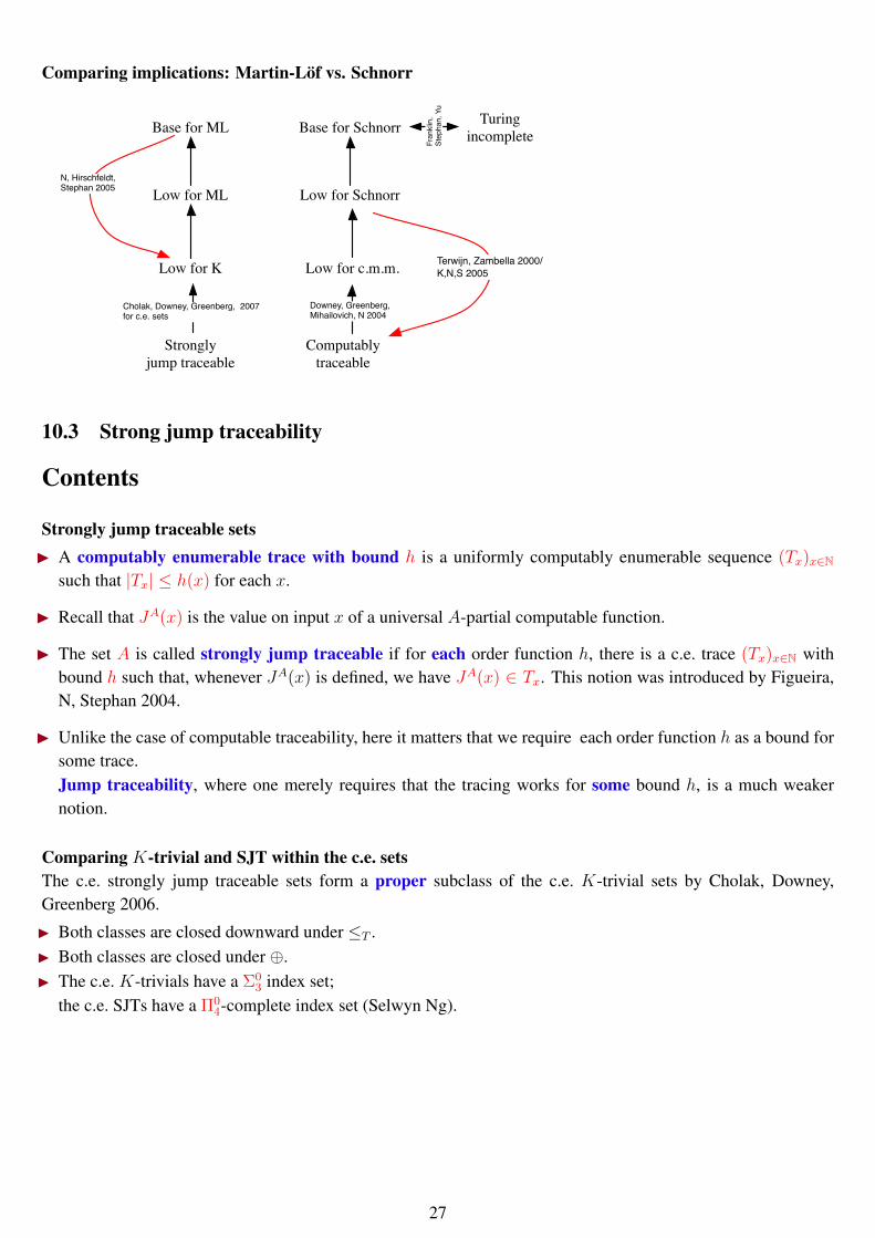
Comparing implications: Martin-Löf vs. Schnorr
Low for K
Low for ML
Base for ML
N, Hirschfeldt, Stephan 2005
Low for c.m.m.
Low for Schnorr
Base for Schnorr
Terwijn, Zambella 2000/K,N,S 2005
Downey, Greenberg,Mihailovich, N 2004
Computablytraceable
TuringincompleteFr
ankli
n,St
epha
n, Y
u
Cholak, Downey, Greenberg, 2007for c.e. sets
Strongly jump traceable
10.3 Strong jump traceability
Contents
Strongly jump traceable setsI A computably enumerable trace with bound h is a uniformly computably enumerable sequence (Tx)x∈N
such that |Tx| ≤ h(x) for each x.
I Recall that JA(x) is the value on input x of a universal A-partial computable function.
I The set A is called strongly jump traceable if for each order function h, there is a c.e. trace (Tx)x∈N withbound h such that, whenever JA(x) is defined, we have JA(x) ∈ Tx. This notion was introduced by Figueira,N, Stephan 2004.
I Unlike the case of computable traceability, here it matters that we require each order function h as a bound forsome trace.Jump traceability, where one merely requires that the tracing works for some bound h, is a much weakernotion.
Comparing K-trivial and SJT within the c.e. setsThe c.e. strongly jump traceable sets form a proper subclass of the c.e. K-trivial sets by Cholak, Downey,Greenberg 2006.
I Both classes are closed downward under ≤T .I Both classes are closed under ⊕.I The c.e. K-trivials have a Σ0
3 index set;the c.e. SJTs have a Π0
4-complete index set (Selwyn Ng).
27
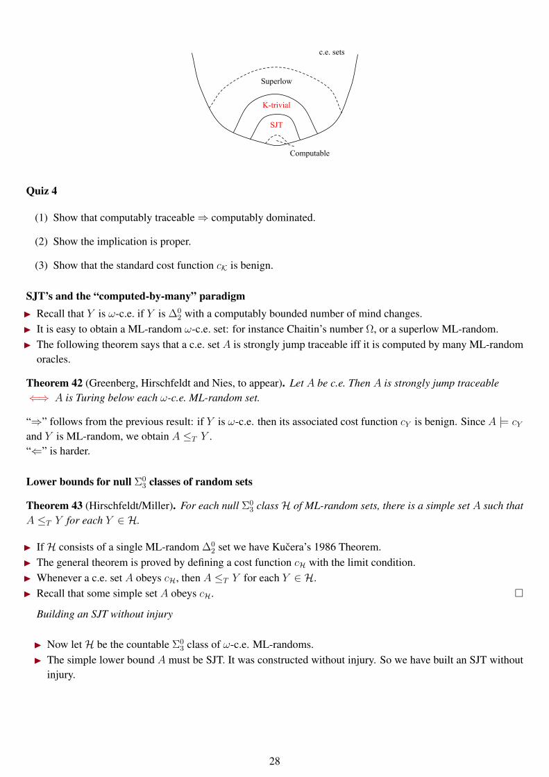
K-trivial
SJT
Computable
Superlow
c.e. sets
Quiz 4
(1) Show that computably traceable⇒ computably dominated.
(2) Show the implication is proper.
(3) Show that the standard cost function cK is benign.
SJT’s and the “computed-by-many” paradigmI Recall that Y is ω-c.e. if Y is ∆0
2 with a computably bounded number of mind changes.I It is easy to obtain a ML-random ω-c.e. set: for instance Chaitin’s number Ω, or a superlow ML-random.I The following theorem says that a c.e. set A is strongly jump traceable iff it is computed by many ML-random
oracles.
Theorem 42 (Greenberg, Hirschfeldt and Nies, to appear). Let A be c.e. Then A is strongly jump traceable⇐⇒ A is Turing below each ω-c.e. ML-random set.
“⇒” follows from the previous result: if Y is ω-c.e. then its associated cost function cY is benign. Since A |= cYand Y is ML-random, we obtain A ≤T Y .“⇐” is harder.
Lower bounds for null Σ03 classes of random sets
Theorem 43 (Hirschfeldt/Miller). For each null Σ03 classH of ML-random sets, there is a simple set A such that
A ≤T Y for each Y ∈ H.
I IfH consists of a single ML-random ∆02 set we have Kucera’s 1986 Theorem.
I The general theorem is proved by defining a cost function cH with the limit condition.I Whenever a c.e. set A obeys cH, then A ≤T Y for each Y ∈ H.I Recall that some simple set A obeys cH.
Building an SJT without injury
I Now letH be the countable Σ03 class of ω-c.e. ML-randoms.
I The simple lower bound A must be SJT. It was constructed without injury. So we have built an SJT withoutinjury.
28
SJT’s and randomness
• Recall that Z is superlow if Z ′ ≤tt ∅′. Dually, we say that Z is superhigh if ∅′′ ≤tt Z′.
• A random set can be superlow (low basis theorem). It can also be superhigh but Turing incomplete (Kuceracoding).
Via randomness we can characterize the c.e. strongly jump traceable sets in various ways.
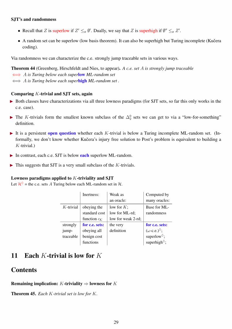
Theorem 44 (Greenberg, Hirschfeldt and Nies, to appear). A c.e. set A is strongly jump traceable⇐⇒ A is Turing below each superlow ML-random set⇐⇒ A is Turing below each superhigh ML-random set .
Comparing K-trivial and SJT sets, againI Both classes have characterizations via all three lowness paradigms (for SJT sets, so far this only works in the
c.e. case).
I The K-trivials form the smallest known subclass of the ∆02 sets we can get to via a “low-for-something”
definition.
I It is a persistent open question whether each K-trivial is below a Turing incomplete ML-random set. (In-formally, we don’t know whether Kucera’s injury free solution to Post’s problem is equivalent to building aK-trivial.)
I In contrast, each c.e. SJT is below each superlow ML-random.
I This suggests that SJT is a very small subclass of the K-trivials.
Lowness paradigms applied to K-triviality and SJTLetH♦ = the c.e. sets A Turing below each ML-random set inH.
Inertness: Weak as Computed byan oracle: many oracles:
K-trivial obeying the low for K; Base for ML-standard cost low for ML-rd; randomnessfunction cK low for weak 2-rd;
strongly for c.e. sets: the very for c.e. sets:jump- obeying all definition (ω-c.e.)♦;traceable benign cost superlow♦;
functions superhigh♦;
11 Each K-trivial is low for K
Contents
Remaining implication: K-triviality⇒ lowness for K
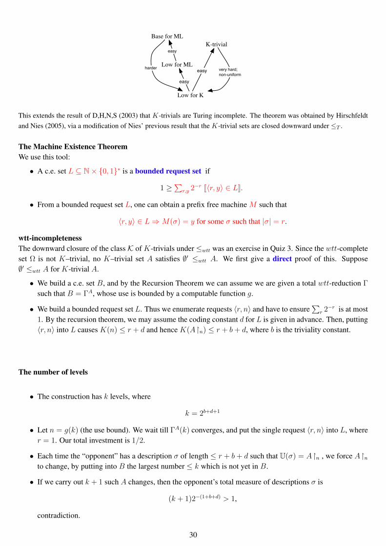
Theorem 45. Each K-trivial set is low for K.
29
Low for K
Low for ML
Base for ML
easy
easy
very hard;non-uniform
K-trivial
easyharder
This extends the result of D,H,N,S (2003) that K-trivials are Turing incomplete. The theorem was obtained by Hirschfeldtand Nies (2005), via a modification of Nies’ previous result that the K-trivial sets are closed downward under ≤T .
The Machine Existence TheoremWe use this tool:
• A c.e. set L ⊆ N× 0, 1∗ is a bounded request set if
1 ≥∑
r,y 2−r [[〈r, y〉 ∈ L]].
• From a bounded request set L, one can obtain a prefix free machine M such that
〈r, y〉 ∈ L⇒M(σ) = y for some σ such that |σ| = r.
wtt-incompletenessThe downward closure of the class K of K-trivials under ≤wtt was an exercise in Quiz 3. Since the wtt-completeset Ω is not K–trivial, no K–trivial set A satisfies ∅′ ≤wtt A. We first give a direct proof of this. Suppose∅′ ≤wtt A for K-trivial A.
• We build a c.e. set B, and by the Recursion Theorem we can assume we are given a total wtt-reduction Γ
such that B = ΓA, whose use is bounded by a computable function g.
• We build a bounded request set L. Thus we enumerate requests 〈r, n〉 and have to ensure∑
r 2−r is at most1. By the recursion theorem, we may assume the coding constant d for L is given in advance. Then, putting〈r, n〉 into L causes K(n) ≤ r + d and hence K(An) ≤ r + b+ d, where b is the triviality constant.
The number of levels
• The construction has k levels, where
k = 2b+d+1
• Let n = g(k) (the use bound). We wait till ΓA(k) converges, and put the single request 〈r, n〉 into L, wherer = 1. Our total investment is 1/2.
• Each time the “opponent” has a description σ of length ≤ r + b+ d such that U(σ) = An , we force Anto change, by putting into B the largest number ≤ k which is not yet in B.
• If we carry out k + 1 such A changes, then the opponent’s total measure of descriptions σ is
(k + 1)2−(1+b+d) > 1,
contradiction.
30
Turing-incompleteness
• Consider the more general result that K-trivial sets are T-incomplete (Downey, Hirschfeldt, N, Stephan,2003). There is no computable bound on the use of ΓA(k).
• The problem now is that the opponent might, before giving a description of As n, move this use beyond n.This deprives us of the possibility to cause further changes of toAn.
• The solution is to carry out many attempts in parallel, based on computations ΓA(m) for different m.
• Each time the use of such a computation changes, the attempt is cancelled. What we placed in L for thisattempt now becomes garbage. We have to ensure that the weight of the garbage does not build up toomuch, otherwise L is not a bounded request set.
More details: j-setsThe following is a way to keep track of the number of times the opponent had to give new descriptions of stringsAs n.Technical detail: we only consider stages (italics) at which A looks K-trivial with constant b up to the previousstage.
I At stage t, a finite set E is a j-set if for each n ∈ E
• first we put a request 〈rn, n〉 into L, and then
• for j times at stages s < t the opponent had to give new descriptions of As n of length rn + b+ d.
I A c.e. set with an enumeration E =⋃Et is a j-set if Et is a j-set at each stage t.
The weight of a k-setThe weight of a set E ⊆ N is
∑2−rn [[n ∈ E]].
Fact 46. If the c.e. set E is a k-set, k = 2b+d+1 as defined above, then the weight of E is at most 1/2.
The reason for this: k times the opponent has to matchour description of n, which has length rn, bya description of a string As n that is by at most b+ d longer.
ProceduresAssume A is K-trivial and Turing complete. As in the wtt-case, we attempt to build a k-set Fk of weight > 1/2
to reach a contradiction.
I Procedure Pj ( 2 ≤ j ≤ k) enumerates a j-set Fj .I The construction begins by calling Pk, which calls Pk−1 many times, and so on down to P2, which enumeratesL (and F2).
Each procedure Pj has rational parameters q, β ∈ [0, 1].
• The goal q is the weight it wants Fj to reach.
• The garbage quota β is how much garbage it can produce (details on garbage later).
When a procedure reaches its goal it returns.
31
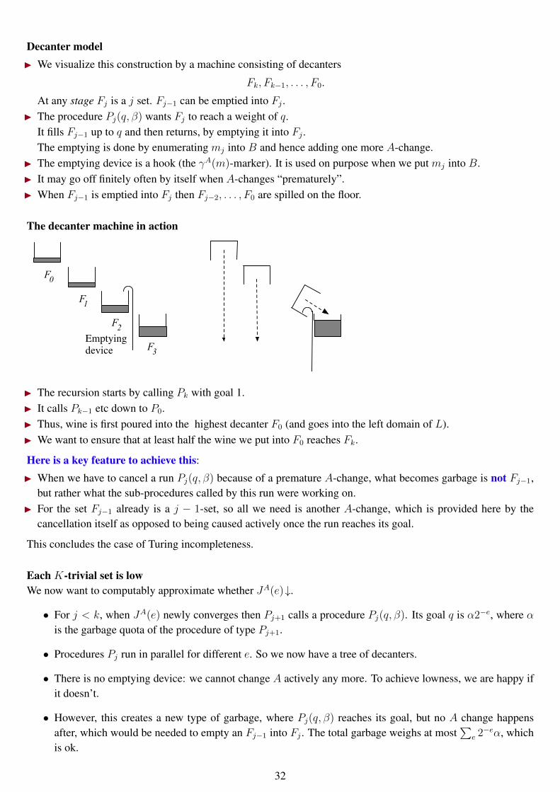
Decanter modelI We visualize this construction by a machine consisting of decanters
Fk, Fk−1, . . . , F0.
At any stage Fj is a j set. Fj−1 can be emptied into Fj .I The procedure Pj(q, β) wants Fj to reach a weight of q.
It fills Fj−1 up to q and then returns, by emptying it into Fj .The emptying is done by enumerating mj into B and hence adding one more A-change.
I The emptying device is a hook (the γA(m)-marker). It is used on purpose when we put mj into B.I It may go off finitely often by itself when A-changes “prematurely”.I When Fj−1 is emptied into Fj then Fj−2, . . . , F0 are spilled on the floor.
The decanter machine in action
Emptying device F3
F0
F1
F2
I The recursion starts by calling Pk with goal 1.I It calls Pk−1 etc down to P0.I Thus, wine is first poured into the highest decanter F0 (and goes into the left domain of L).I We want to ensure that at least half the wine we put into F0 reaches Fk.
Here is a key feature to achieve this:
I When we have to cancel a run Pj(q, β) because of a premature A-change, what becomes garbage is not Fj−1,but rather what the sub-procedures called by this run were working on.
I For the set Fj−1 already is a j − 1-set, so all we need is another A-change, which is provided here by thecancellation itself as opposed to being caused actively once the run reaches its goal.
This concludes the case of Turing incompleteness.
Each K-trivial set is lowWe now want to computably approximate whether JA(e)↓.
• For j < k, when JA(e) newly converges then Pj+1 calls a procedure Pj(q, β). Its goal q is α2−e, where αis the garbage quota of the procedure of type Pj+1.
• Procedures Pj run in parallel for different e. So we now have a tree of decanters.
• There is no emptying device: we cannot change A actively any more. To achieve lowness, we are happy ifit doesn’t.
• However, this creates a new type of garbage, where Pj(q, β) reaches its goal, but no A change happensafter, which would be needed to empty an Fj−1 into Fj . The total garbage weighs at most
∑e 2−eα, which
is ok.
32
A tree of runs
. . .
. . .
. . .
. . .
golden run
......
.........
......
...
. . .
. . .
......
......
......
. . .
. . .
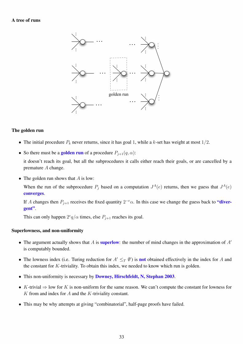
The golden run
• The initial procedure Pk never returns, since it has goal 1, while a k-set has weight at most 1/2.
• So there must be a golden run of a procedure Pj+1(q, α):
it doesn’t reach its goal, but all the subprocedures it calls either reach their goals, or are cancelled by apremature A change.
• The golden run shows that A is low:
When the run of the subprocedure Pj based on a computation JA(e) returns, then we guess that JA(e)
converges.
If A changes then Pj+1 receives the fixed quantity 2−eα. In this case we change the guess back to “diver-gent”.
This can only happen 2eq/α times, else Pj+1 reaches its goal.
Superlowness, and non-uniformity
• The argument actually shows that A is superlow: the number of mind changes in the approximation of A′
is computably bounded.
• The lowness index (i.e. Turing reduction for A′ ≤T ∅′) is not obtained effectively in the index for A andthe constant for K-triviality. To obtain this index, we needed to know which run is golden.
• This non-uniformity is necessary by Downey, Hirschfeldt, N, Stephan 2003.
• K-trivial⇒ low for K is non-uniform for the same reason. We can’t compute the constant for lowness forK from and index for A and the K-triviality constant.
• This may be why attempts at giving “combinatorial”, half-page proofs have failed.
33
Proving the full resultWe now show that K-trivial⇒ low for K.
• For j < k a procedure Pj(q, β) is started when UA(σ) = y newly converges. Its goal q is α2−|σ|.
• We call, in parallel, procedures based on different inputs σ. So we again have a tree of decanters.
• Via a golden run Pj+1, we show that A is low for K. When Pj(q, β) associated with UA(σ) = y returns,we have the right to enumerate a request 〈|σ|+ c, y〉 into a set W (c is some constant).
• Every A change means useless weight in W , since we issued request for a wrong computation UA(σ). Thefact that Pj+1 does not reach its goal implies that the total weight is bounded. Hence W is a boundedrequest set.
Cost function characterization of the K-trivialsRecall: the cost function cK for K-triviality is given by
cK(x, s) =∑s
i=x+1 2−Ks(i).
Theorem 47 (Nies 05). A is K-trivial ⇐⇒some computable approximation of A obeys cK.
We have already done “⇐”. For “⇒” one uses the golden run.
Corollary 48. For each K-trivial A there is a c.e. K-trivial set D ≥tt A.
D is the change set 〈x, i〉 : A(x) changes at least i times. One verifies that D obeys cK as well.Actually, this works for any cost function in place of cK.
Summary of Lecture 3I We have studied versions of ML-randomness and K based on Π1
1 sets.I We have defined the NCR sets, a further notion of being far from random.I Traceability is a meta-concept leading to interesting lowness properties.I Computable traceability characterizes lowness for Schnorr randomness.I The c.e. strongly jump traceable sets form an interesting, very small subclass of the c.e. K-trivial sets. They
can be naturally characterized via the “computed-by-many” paradigm.I The decanter method shows each K-trivial is Turing incomplete. Adding the non-uniform golden run method
shows that each K-trivial is in fact low for K.
34