Applying Machine Learning to Identify Regimes for Asset ... · Princeton University ORFE Report Improve diversification -- get paid to take on risks Help explain newer securities

APPLYING MACHINE LEARNING TO

IDENTIFY REGIMES FOR ASSET ALLOCATION AND ALM

PROFESSOR JOHN M. MULVEY OPERATIONS RESEARCH AND FINANCIAL ENGINEERING

BENDHEIM CENTER FOR FINANCE PRINCETON UNIVERSITY

OCTOBER 5, 2016

Princeton University ORFE Report

1. Factor investing for asset allocation (feature selection)

2. Motive regimes and apply 2-regime simulation to a university endowment

3. Factor investing for ALM and a large pension plan study

4. Future steps

2

Agenda

10/5/16


Improve diversification -- get paid to take on risks

Help explain newer securities and asset categories • Examples:

o Junk bonds

o FTSE Dynamic Commodity Index (long short commodity via futures)

Assist during crash periods when contagion is present

Intensive search for higher returns to achieve goals and meet liabilities

3

Factor Investing

10/5/16


Danish Pension System ATP – Factors for Assets (Ang)

Liability-related factors – Real economic growth, inflation (hard to link to asset returns)

4

Example: Factors as Building Blocks (critical ingredients)

10/5/16


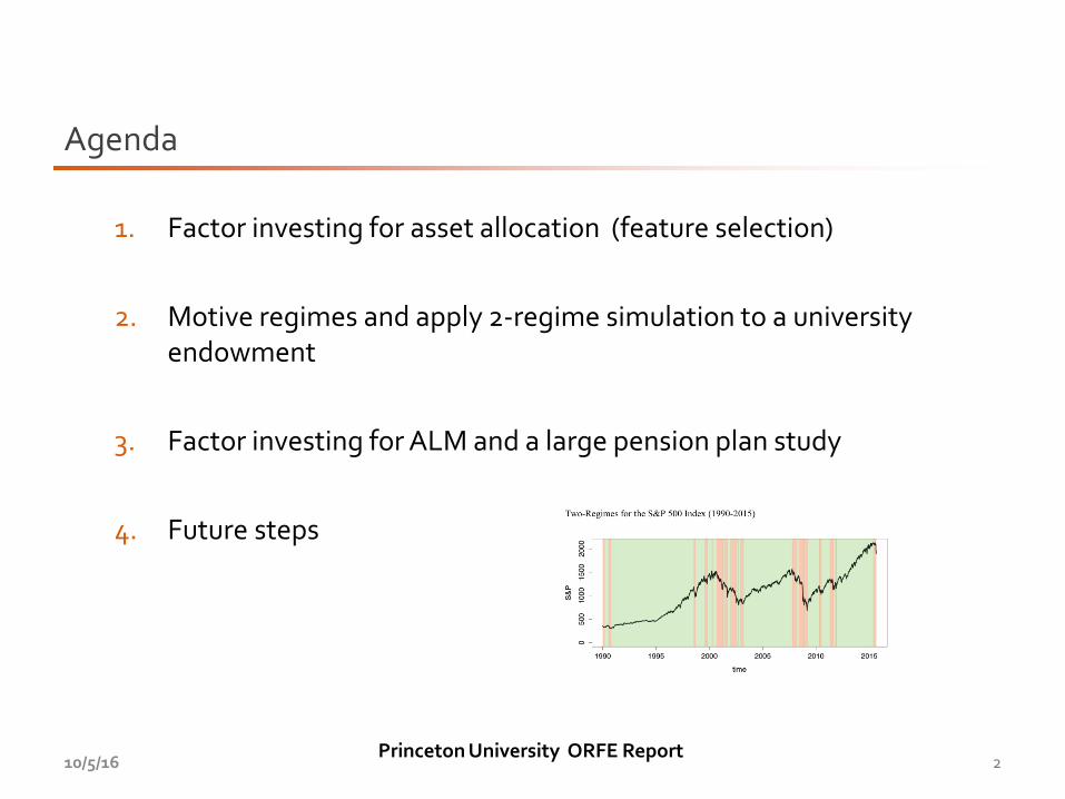
Many institutional investors have made the shift to “alternative” asset categories

• 57% on average for U.S. endowments above $1 B

• Main categories: private equity, real assets, hedge funds

• There is great diversity in this domain

• The newer asset categories capture many types of risks

5

Why Factor Investing?

10/5/16

Princeton University ORFE Report 6

Average Allocation Across University Endowments

10/5/16

Asset Allocation for U.S. Colleges and Universities 2014 (NACUBO 2015)

Survey Average Endowments over $1b Equities 36% 31% Domestic Equities 17% 13% International Equities 19% 18% Fixed Income 9% 8% Alternatives 51% 57% Short-term 4% 4% securities/ cash/ other


Examples of Subcategories in Hedge Fund Land

10/5/16

Institutions Subdividing Absolute Return/Hedge Fund Categories

Institution # Equity-related Hedge Fund

Other Categories Category

Georgia Institute of Technology 2 L/S equity hedge funds Multi-strategy hedge funds

Williams College 2 Global long/short equity Absolute return Marketable strategies: Credit/absolute

U. Illinois Foundation 2 Marketable strategies: Hedged equity return/ distressed

U. North Carolina at Chapel Hill 2 L/S equity Diversifying strategies Absolute return Strategies, Cross-Asset

University of California 3 Opportunistic equity Class Strategy

Credit-related fixed income, Investment Developed country equity, Emerging grade fixed income, Real estate, Natural

University of Texas System 6 markets resources

University of Washington 2 Capital appreciation: Opportunistic Capital preservation: Absolute return Hedged strategies: Credit relate, Hedged

Pennsylvania State University 3 Hedged strategies: Equity related strategies: other

The Ohio State University 2 Long/short equities Relative valuejmacro, Credit funds

University of Virginia 2 Long/short equity Marketable alternatives & Credit


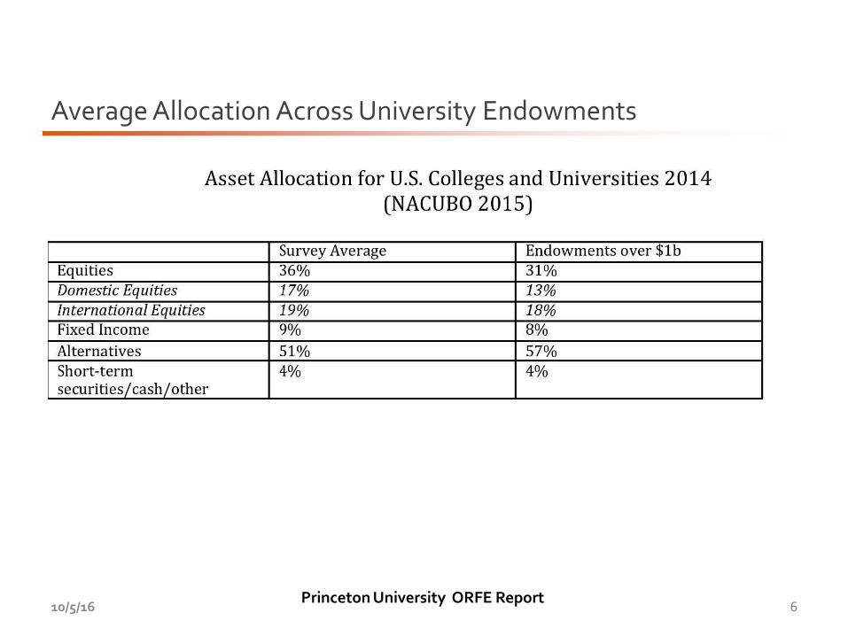
An Example of the Diversity in Defining Asset Categories

10/5/16

Duke's Target Asset Allocation & Asset Category Descriptions (June 30 2014) Source: Duke (2014)

Equity-49%

Public Equity Private Equity Commodityrelated equities

l Me Uoi,mHy l I

Private investments in energy, power, infrastructure &

timber

Real estate-11%

Direct commodity exposure

Corporates, Bank Debt, assetbackeds etc

public obligations, incl.

treasuries & agencies

Public obligations, incl.

treasuries & agencies


Purely statistical factors • Factor analysis, principle component analysis

Fundamental macro economic • Chen, Roll, and Ross

– Maturity premium (long- short government bonds), expected inflation, unexpected inflation, industrial production growth, and default premium (corporate high versus low grade bonds)

Micro factors • Fama and French

– Equity markets risks, small minus large stock returns, value minus growth

– Profitability (high-low profit), and investment (conservative-aggressive investment)

– Momentum, and low volatility

Number of factors determined by sensitivity analysis • Most studies have shown that about 5 factors are best (little improvement above 5 for

equities)

9

Alternative Factor Approaches (Feature selection in machine learning)

10/5/16


10

Factor Loadings for Harvard Endowment

10/5/16

Apply cross validation from machine learning

Motivate Regimes with a Study of a University Endowment


Most Hedge Funds Experienced Contagion during 2008 Crash –> massive change in covariance matrix

10/5/16

Most Hedge Funds Experienced the Classic Pattern of Contagion during the 2008 Crash Note: stark differences between normal2001-2007 period (left side) and crash 2008 period (right side)

(heavy line = correlation > .5; light line = correlation between .2 and .5; no line = correlation < .2)

o:-g;.g ........ l.1S'IIo

"5r------.::. r £-~~~fT~-~500 -~-

,_......, ··- r.....,....,. .. ..., = 1.12'4

-_ .. ...-)


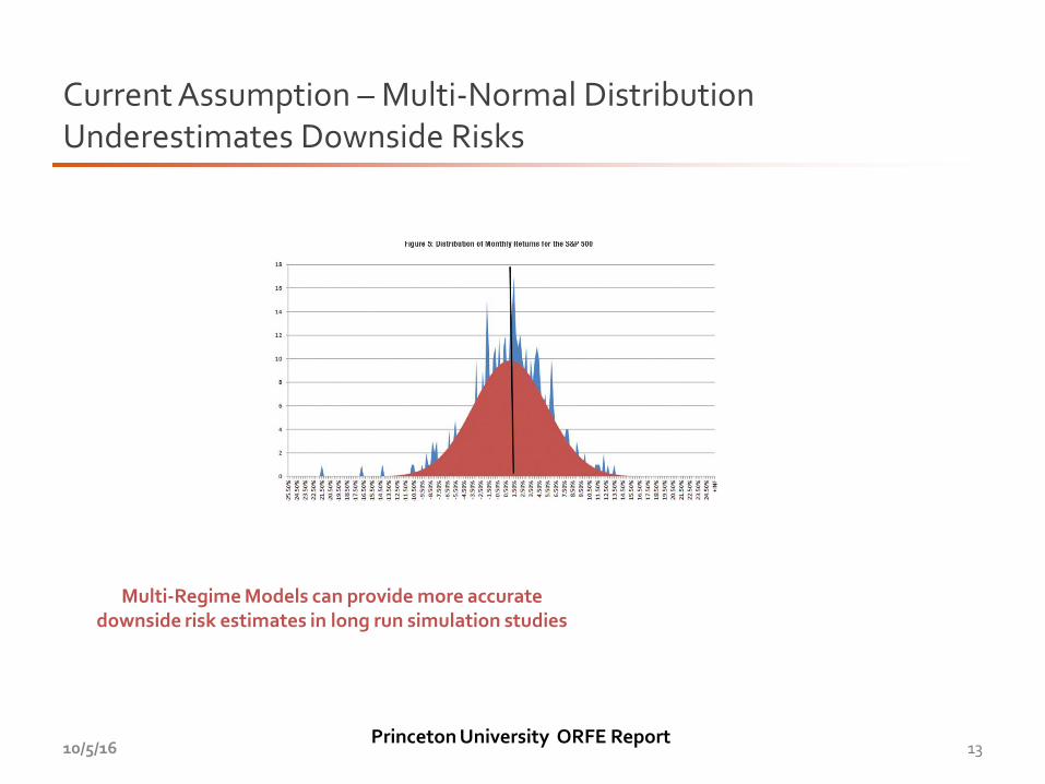
Current Assumption – Multi-Normal Distribution Underestimates Downside Risks

10/5/16

Multi-Regime Models can provide more accurate downside risk estimates in long run simulation studies


14

Identify Two Regimes via Trend Filtering Algorithm*

10/5/16

*See appendix

Two-Regimes for the S&P 500 Index (1990-2015)

0 0 0 C\1

0 0 LO

a.. 0 ~ 0 (/) 0

T""

8 LO

0

1990 1995 2000 2005 2010 2015

time


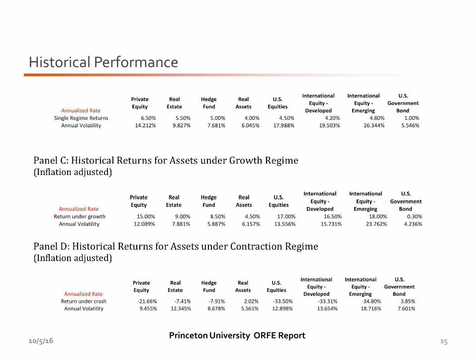
Historical Performance

10/5/16

Private Real Hedge Real u.s.

Annualized Rate Equity Estate Fund Assets Equities

Single Regime Returns 6.50% 5.50% 5.00% 4.00% 4.50% Annual Volat ility 14.212% 9 .827% 7.681% 6.045% 17.988%

Panel C: Historical Returns for Assets under Growth Regime (Inflation adjusted)

Private Real Hedge Real u.s.

Annualized Rate Equity Estate Fund Assets Equities

Return under growth 15.00% 9.00% 8.50% 4.50% 17.00% Annual Volat ility 12.089% 7.881% 5.887% 6.157% 13.556%

International Equity-

Developed 4.20%

19.503%

International

Equity-

Developed

16.50% 15.731%

Panel D: Historical Returns for Assets under Contraction Regime (Inflation adjusted)

Private Real Hedge Real u.s. International

Equity Estate Fund Assets Equities Equity-

Annualized Rate Developed Return under crash -21.66% -7.41% -7.91% 2.02% -33.50% -33.31%

Annual Volatility 9.455% 12.345% 8.678% 5.561% 12.898% 13.654%

International u.s. Equity- Government

Emerging Bond 4.80% 1.00%

26.344% 5.546%


Emerging Bond

18.00% 0 .30% 23.762% 4.236%


Emerging Bond -34.80% 3.85% 18.716% 7.601%


Transition Matrix

10/5/16

Employ these probabilities in the two-regime

simulation


Single regime: select asset returns each period via a single multi-normal distribution; pay operating budget at 4% of capital (averaged over 4 years)

Two regime: start with non-crash distribution; switch between non-crash and crash each quarter depending upon transition probability; pay operating budget the same as above

The two regime model more accurately projects the worst events (left tails) than the single regime approach

17

Multi-Period Simulation

10/5/16


Forward Looking Simulation – Sample Path

10/5/16

A Representative Scenario Path over the 50-Year Planning Horizon (S&P 500 Index)

12

10

r-0

0

11

/ I'+ N I 10 15

~ I~ 20 25

Tlfl'le(year)

~

30

/ /

,v 35 40

I 50


Compare Single and Two-Regime Models

10/5/16

Summary Statistics for Baseline Monte Carlo Simulations ( 4°/o Target Spending Target)

Without Spending

spending-cut Cut by rule 20%

Simulation Results 1-Regime 2-Regime 1-Regime 2-Regime

Crash Prob, 5 years 10.3% 18.4% 10.3% 18.4% Crash Prob, 10 years 20.5% 31.8% 20.0% 31.5% Crash Prob, 50 years 4.9% 19.9% 2.2% 13.1%

mean-S years 1.0644 1.0780 1.0644 1.0780 mean-10 years 1.1635 1.1793 1.1692 1.1879 mean-20 years 1.3998 1.4230 1.4173 1.4514 mean-50 years 2.6630 2.6197 2.7152 2.7147

#of simulations 10000 10000 10000 10000 Average% time in "adverse" 2.88% 5.60% 2.22% 4.60%


Advantages of Reducing Spending

10/5/16

Panel B : Performance Statistics for 3.5o/o Spending Target Without Spending

spending-cut Cut by rule 25%

Simulation Results 1-Regime 2-Regime 1-Regime 2-Regime

Crash Prob, 5 years 8.3% 16.3% 8.3% 16.3%

Crash Prob, 10 years 14.6% 26.6% 14.4% 26.4%

Crash Prob, SO years 1.2% 8.5% 0.4% 5.6%

mean-S years 1.0977 1.1112 1.0977 1.1112

mean-10 years 1.2421 1.2609 1.2462 1.2680

mean-20 years 1.5883 1.6267 1.6018 1.6499 mean-50 years 3.6169 3.6499 3.6585 3.7310

#of simulations 10000 10000 10000 10000

Average% t ime in "adverse" 1.39% 3.41% 1.06% 2.68%

Factor Investing for a Large Pension System via ALM

Mention attention to liabilities – CFA level 3


1. Assets returns are driven by short and mid-term factors (interest rates, risk

premium, cash flows, and micro factors such as momentum, value and so on)

2. Liabilities are driven by mid to long term factors

3. Longevity issues

22

Difficulties Explaining Assets and Liabilities via Common Factors

10/5/16

Market factors (short horizon), Macro-economic factors (intermediate horizon), demographic factors (long horizon)


Two macro-economic factors that affect liability cash flows are:

• Growth – Real Gross Domestic Product ( GDP)

• Inflation

Impact on salaries and retirement benefits

Assumption: liabilities are discounted at the blended return rate (for now)

23

Macro-Economic Factors and Pension Liabilities

10/5/16


Pension Payroll and GDP showed a strong relationship

24

History - Pension Payroll, GDP and US Inflation

10/5/16

.

$1

$2

$3

$4

1987 1992 1997 2003 2008 2014 Valuation Year


1. Consistency between asset performance and changes in liability cash flows

1. Improved estimates of downside risks

1. Enhanced asset performance (possibly)

2. Streamlined estimates of liability cash flows

25

Potential Advantages of Regime-Aware ALM

10/5/16


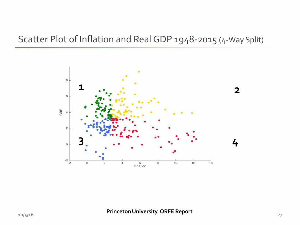
Assume that the current state of the economy is defined by Real GDP growth and inflation:

26

An Illustrative Example

10/5/16

GDP Growth

Inflation

GDP Growth: High Inflation: High

Economic State 2

GDP Growth: Low Inflation: High

Economic State 4

GDP Growth: Low Inflation: Low

Economic State 3

GDP Growth: High Inflation: Low

Economic State 1


Scatter Plot of Inflation and Real GDP 1948-2015 (4-Way Split)

10/5/16

1

4 3

2


Historical Patterns (time series of inflation and real GDP)

10/5/16

I~

12

10

8

l ..... e

4

2

0

·2

.... 10!>0 1900 1970


Four Regimes are Stable Across Time

10/5/16

Time Period 1948-2014

Frequency Quarterly

Regime 1 Regime 2 Regime 3 Regime 4

Regime 1 0.83 0.09 O.Q7 0.01

Regime 2 0.05 0.83 0.00 0.13

Regime 3 0.10 0.00 0 .84 0.06

Regime 4 0.04 0 .07 0.08 0.80


Performance of Asset Categories

10/5/16

Real Returns ofMajor Asset Categories (1973-2015 monthly) I

Geometric Mean of Return (Annually)

U.S.Equity lnti.Equity

5.8354% 4.6518%


U.S.Treasury

4.0300% Corp. Bond

3.5651%

Real Estate

5.3212%

Commodity

2.4234%

TIPS

2.9045%

U.S.Equity lnt i.Equity U.S.Treasury Corp. Bond Real Estate Commodity TIPS

Regime 1 15.2834% 13.4923% 6.9086% 5.1891% 9.1384% 9.7553% 3.7975%

Regime 2 0.8939% 6.4105% -0.1339% 1.4991% 3.9968% 4.7818% 1.0627%

Regime 3 11.0503% 10.6285% 5.1594% 7.4233% 13.7547% -0.8822% 6.1820% Regime 4 -2.8658% -10.2222% 4.3173% 0.3051% -4.6992% -3.4542% 0.6718%

Risk Free

0.6919%

Risk Free

1.4420%

0.7616%

0.2001% 0.3682%

Regime 1 = growth+ and inflation-, Regime 2= growth+, inflation+, Regime 3 = growth-, inflation-, Regime 4 = growth-, inflation+


Equity Micro-Factor Performance

10/5/16

Real Return of Equity Micro-Factors over Four Regimes- 1970-2015 monthly

Geometric Mean of Return {Quarterly} High Low High Low High Low

I High Value I Low Value I High Vol Low Vol I Investment I Investment I Profitability I Profitability I Momentum I Momentum I Regime 1 5.36% 4.20% 4.73% 4.08% 4.37% 4.99% 5.42% 4.30% 6.36% 3.53%

Regime 2 3.40% 0.97% 1.91% 2.19% 1.44% 2.49% 1.96% 1.82% 2.51% 1.23%

Regime 3 2.86% 0.97% 1.01% 2.19% 0.78% 2.54% 2.39% 1.23% 1.12% 1.88%

Regime 4 2.78% 0.86% 2.14% 1.63% 1.63% 2.26% 1.82% 2.01% 2.48% 1.22%


Motivate – long/short versions to improve diversification

32

Equity Segments are Highly Correlated

10/5/16


33

Comparing Traditional MVO and Regime-Aware Approach

10/5/16

Inputs to a Markowitz Portfolio Model January 1973-December 2007, Real Monthly Returns

Geometric Mean of Return (Monthly) U.S.Equity Inti. Equity U.S.Treasury Corp. Bond Real Estate Commodity TIPS Risk Free

0.4803% 0.4870% 0.2995% 0.2806% 0.4222% 0.4727% 0.2507% 0.0968%

Conditional Value at Risk (Monthly) U.S.Equity Inti. Equity U.S.Treasury Corp. Bond Real Estate Commodity TIPS Risk Free

-10.0627% -10.6460% -5.9763% -4.2674% -10.7883% -11.5732% -6.8351% -0.3874%

Volatility (Monthly) U.S.Equity Inti. Equity U.S.Treasury Corp. Bond Real Estate Commodity TIPS Risk Free

0.044211 0.047802 0.030183 0.021728 0.045102 0.055778 0.028858 0.002063

Sharpe Ratio (Monthly) U.S.Equity Inti. Equity U.S.Treasury Corp. Bond Real Estate Commodity TIPS Risk Free

0.086752 0.081635 0.067182 0.084619 0.072162 0.067397 0.053333 0.000000

Correlation U.S.Equity Inti. Equity U .S.Treasury Corp. Bond Real Estate Commodity TIPS Risk Free

U.S.Equity 1.000000 0.574599 0.211152 0.236128 0.565631 0.005373 0.114511 0.011030 lnt i.Equity 0.574599 1.000000 0.134243 0.204139 0.387313 0.062845 0.070981 0.022911 U.S.Treasur 0.211152 0.134243 1.000000 0.741640 0.238839 -0.049413 0.481781 0.174982 Corp. Bond 0.236128 0.204139 0.741640 1.000000 0.288717 -0.050624 0.387406 0.197569 Real Estate 0.565631 0.387313 0.238839 0.288717 1.000000 -0.041503 0.214121 -0.034849 Com mod it\ 0.005373 0.062845 -0.049413 -0.050624 -0.041503 1.000000 0.101095 -0.015984 TIPS 0.114511 0.070981 0.481781 0.387406 0.214121 0.101095 1.000000 0.096095 Risk Free 0.011030 0.022911 0.174982 0.197569 -0.034849 -0.015984 0.096095 1.000000


34

Comparing Traditional MVO and Regime-Aware Approach

10/5/16

Performance of Assets Under the Four Regimes January 1973 to December 2007

Geometric Mean of Return (Monthly) U.S.Equity lnti.Equity U.S.Treasury Corp. Bond Real Estate Commodity TIPS Risk Free

Regime 1 1.1820% 1.1216% 0.4543% 0.3829% 0.6396% 1.1698% 0.3033% 0.1574% Regime 2 0.0742% 0.5191% ·0.0112% 0.1036% 0.3271% 0.3900% 0.0881% 0.0632% Regime 3 0.5105% 0.6285% 0.6368% 0.5022% 0.7955% 0.0284% 0.6426% 0.0943% Regime 4 0.2245% -Q.2829% 0.2715% 0.2300% 0.0574% 0.1740% 0.1165% 0.0759%


U.S. Equity lnti.Equity U.S. Treasury Corp.Bond Real Estate Commodity TIPS Risk Free

Regime 1 15.1435% 14.3208% 5.5896% 4.6924% 7.9512% 14.9772% 3.7006% 1.9056% Regime 2 0.8939% 6.4105% -Q.1339% 1.2503% 3.9968% 4.7818% 1.0627% 0.7616% Regime 3 6.3007% 7.8078% 7.9149% 6.1962% 9.9747% 0.3409% 7.9896% 1.1377% Regime4 2.7279% -3.3423% 3.3074% 2.7946% 0.6906% 2.1084% 1.4074% 0.9152%

Conditional Value at Risk (Monthly) U.S.Equity lnti.Equity U.S. Treasury Corp.Bond Real Estate Commodity TIPS Risk Free

Regime 1 -5.4773% -7.0090% -4.7597% -2.6150% -6.5103% -8.4059% -3.8300% -0.1358% Regime 2 -11.7270% -11.3778% -4.9681% -3.8713% -10.8949% -11.0935% -7.0140% -0.2242% Regime 3 -9.6752% -11.2141% -6.6980% -2.4451% -8.7136% -11.6188% -3.2554% -0.1359% Regime 4 -10.8876% -11.9761% -7.0830% -6.8815% -14.0816% -14.5317% -8.9285% -0.5232%

Conditional Value at Risk {Annually) U.S.Equity lnti.Equity U.S.Treasury Corp.Bond Real Estate Commodity TIPS Risk Free

Regime 1 -49.1331% -58.1890% -44.3009% -27.2381% -55.4172% -65.1333% -37.4140% -1.6173% Regime 2 -77.6161% -76.5303% -45.7459% -37.7359% -74.9485% -75.6105% -58.2161% -2.6576% Regime 3 -70.5094% -76.0045% -56.4795% -25.6995% -66.5133% -77.2848% -32.7766% -1.6182% Regime 4 -74.9241% -78.3626% -58.5865% -57.4960% -83.8179% -84.8063% -67.4469% -6.1009%

Volatility (Monthly) U.S.Equity lnti.Equity U.S. Treasury Corp.Bond Real Estate Commodity TIPS Risk Free

Regime 1 0.036762 0.040043 0.024361 0.014356 0.034961 0.048S38 0.018276 0.001563 Regime 2 0.044392 0.045772 0.026912 0.018935 0.042762 0.057525 0.027643 0.001952 Regime 3 0.042659 0.050499 0.032279 0.014211 0.036556 0.052504 0.021081 0.001437 Regime 4 0.051203 0.054603 0.036895 0.032596 0.060046 0.062507 0.041122 0.002771

Sharpe Ratio (Monthly) U.S.Equity lnti.Equity U.5.Treasury Corp.Bond Real Estate Commodity TIPS Risk Free

Regime 1 0.278706 0.240775 0.121850 0.157036 0.137920 0.208577 0.079799 0.000000 Regime 2 0.002465 0.099597 -0.027649 0.021309 0.061706 0.056803 0.009002 0.000000 Regime 3 0.097557 0.105774 0.168056 0.287058 0.191804 -o.012562 0.260078 0.000000 Regime 4 0.029019 -0.065716 0.053010 0.047248 -0.003093 0.015691 0.009871 0.000000


35

Compare Traditional MVO and Regime-Aware Approach

10/5/16

Opt Portfolios U.S.Equity Inti. Equity U.S. Treasury Corp. Bond Real Estate Commodity TIPS Risk Free Full period 18.89% 14.70% 8.30% 26.28% 8.73% 23.10% 0.00% 0.00% Regime 3 0.00% 7.54% 26.28% 0.00% 27.39% 0.00% 38.79% 0.00%

Exhibit 22 Total Return for the MVO allocation and the Regime-Aware allocation

Full Period Regime 3 Aware

2008 -30.25o/o -10.9% 2008-2014 5.6% 43.1%

Volatility 8.15% 8.43%

Future Directions


Identify regimes via alternative approaches

Evaluate performance of assets and micro-factors over the stated regimes • Factors (features) over regimes

• Apply machine learning as appropriate

Develop robust allocations in light of current and projected regimes (over the mid-term)

37

Current Research

10/5/16


38

Alternative Regime Definitions

10/5/16

Defining Five Economic Regimes based on Machine Learning Methods

10

8

6

c._ 0 4 (!)

2

0

• •

• • • • • • •• • •

•

•

• ~ .. .., .. . i· .. . . . .. . -: . . . ~ ...... ... . ~ .. , ~-·

• • ••• flt'ta. • ••••• . . .:.-.. . • ef•.. I e e • •. , ., ·.!!"1 ··· . . . ......., .. .,. • • •

• ~;- ••• !. .C• •

• • • • •

• • • • • •

• • • ••

•

•

••

•

• •

• •

• •

• • •• • •

• •• -2L-----L---~L-----L-----L-----L-----~----~--~

·2 0 2 6 Inflation

8 10 12 14


39

A Crash Regime Looks Sensible

10/5/16

Historical Record of Five Regimes 1948-2015

14------

12

10

4

2

0

1960 1970 1980 1990 2000 2010 Year


Mulvey, J.M. and M. Holen, “What Can We Learn from University Endowments: Insights from Self-Reports,” Journal of Investment Consulting, 2017 (to appear).

“Identifying Economic Regimes: Reducing Downside Risks for University Endowments and Foundations, Journal of Portfolio Management, Fall 2016.

“A Nonparametric Smoothing Approach to Financial Market Regime Identification,” Princeton University Report, J. Mulvey, H. Liu, and T. Zhang, August 2015.

_____________________________________________________________________________________

“Dynamic Asset Allocation for Varied Financial Markets under Regime Switching Framework,” European Journal of Operational Research ,G. Bae., W. Kim, and J. Mulvey 2013.

“Assisting Defined-Benefit Pension Plans,” Operations Research, 2009 (with K. Simsek, Z. Zhang, and F. Fabozzi).

Towers Watson, Global Pension Asset Study 2015.

The Elements of Machine Learning, 2nd Edition, T. Hastie, R. Tibshirani, and J. Friedman (2009).

40

References

10/5/16

Appendix


Global Pension Assets Study 2015 (Towers Watson)

10/5/16

Austral ia 1,675 113.0% Brazil ' 268 12.0% Canada 1,526 85.1% France 171 5.9%

German~ 520 13.6% Hong Kong 120 41.2%

Ireland 132 53.7% Japan3 2,862 60.0%

Malaysia 205 60.7% Mexico 190 14.6%

Netherlands 1,457 165.5% South Africa 234 68.6% South Korea 511 35.3% Switzerland" 823 121.2%

UK 3,309 11 6.2% US5 22,117 127.0%

Total 36,119 84.4%


43

Trend Filtering Algorithm

10/5/16

A deta.ikd formulaction of the trend illMring is sa fcillm\'li. Let Y = (Y1, .. . , Y,.)'J" E R"

deno-oo t.he price of a. series at n ~y spaced time pointl:l. For .a given intJi!ger k, the gEDleTa!

form of a toond Dltmiog estimator ji = (#1 •... ,i,_)'r E R,... is d'e:fined SB tJlm solution to the

following penaJi.zed optim.i.zatjon problem:

fi = a.r.gmjn IIY- Pll~ + J..IIDt'=+L).Btl •• (2.I) ,a\G:F

where A 2: 11) is a regn.]ArizAtion pa.mmemr, and D l"=t-l) E R( .. -Ji:-l)x .. chmO'I:.es tbe operuor

for co:mputin,g the (1: + 1}-th order dilcret.e darivath'B. !Fbr 8XAIJ!I.ple, whsn k = 0 and k = 1,

I -1 11) 0 0 I -2 1 0 0

D(L) = 0 1 -1 0 0 .JiJC2l = 0 I -2 0 0

0 11) 0 1!. -I [) 0 0 -2 1



10/5/16

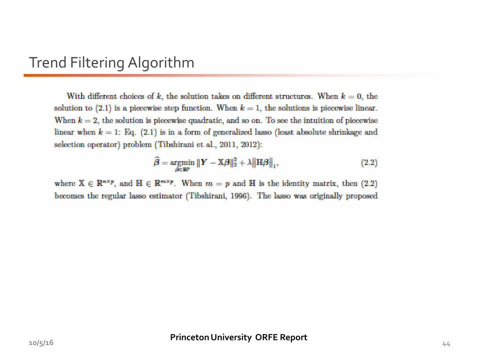
\Vith different choica~ oJ k, the eoluti-cn t.a.kr:9 on diffsrent s.tructmc;. '\Yhcn ' = 0', the solution to (:2.1) is a p]rrew:isc step fucct ion. \i\'hm k = 1: tha :solutiow is piecGwiso lio.ear.

\Vhm k = 2, the solntion is pJCC!.1wise quadratic, and :so on. To see the intuition of piccev,iae

linGSI when k = 1: Eq. (:2.1} is in a form of gcnerallzed lasso (least abiolute ~c and

seloction oparator) problem (Tibahirani ~at aiL, 2011, 2(112):

where X E R~~~xp: a.nd H E Rm.x;p _ \\"hen m = p and H is the identity IIJAt.Tix, then (2.2)

becomes the regular Jasso £5timator (T~b.shirani, 1 OOG). The las:o w~ originally propct.SEd



10/5/16

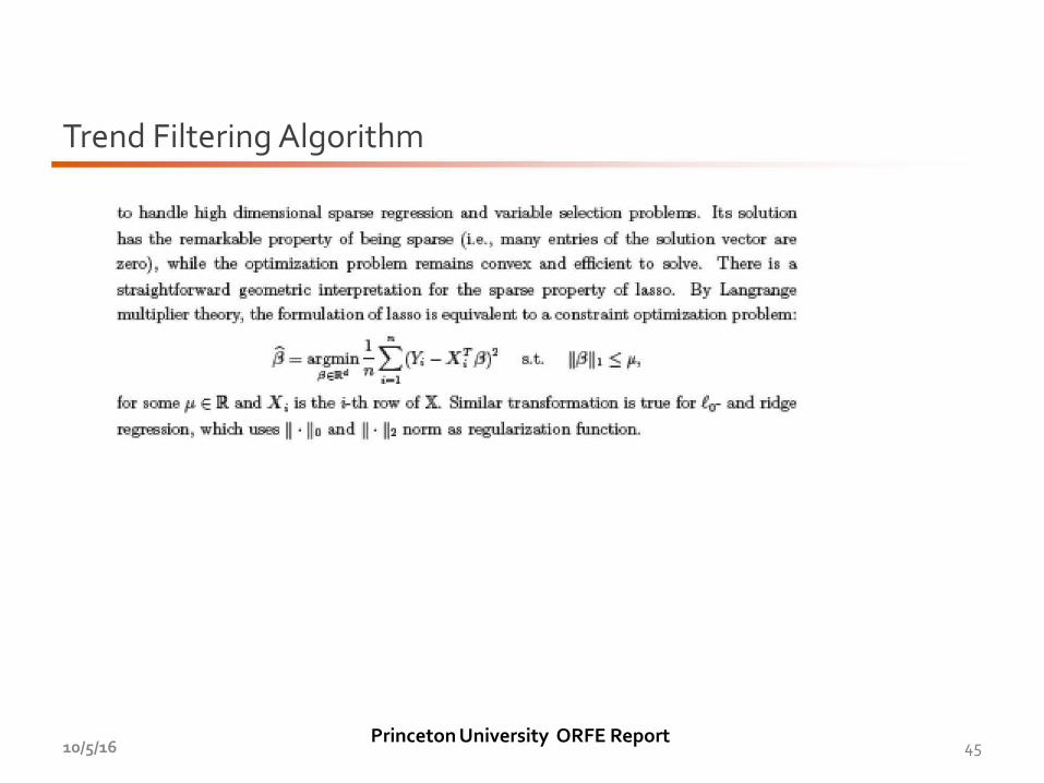
to handle high dimeruionaJ. erparaa repE&Il.om and~ aalectio:D probleJIE. Ita S®lution

has 'the remMlt:able property of 'being sparse (Le., illla'llj" entries of tihe oohlli:don veato:r are

zero) ; while the optUir:lliz!Udnn probia:m i['8]IIalna coll'i'eX amd efficient to IDlve. The:re :liB a

straig.htforwud geometric interpreta.ti.-On for the sp8.:1'88 property of lu11o.. Hy Lmgrange

ml!ll.tiplier th€10F.}', the fm:m:ula.ti.on of lu11o ill equivalent to a. coDBtraint optimi.z:ati.on problem:

1 ,. jj = a.rgnnin - L ~ -xr Pi at.. IIJ3111 < ,,

psa.d n i-1

ioo &Ollile I' E Ill a.nd Xi is the i-th row oo X. S:tmil&r tr~ticm is t.me fm flT and rldge

regr.:.smon, whim 1!lae8 II · II o amd II · ll2 nmm ea mgula.rization fu.nctimL

Documents

Applying Machine Learning to Identify Regimes for Asset ... · Princeton University ORFE Report Improve diversification -- get paid to take on risks Help explain newer securities