Embed Size (px)
Citation preview
(IJARAI) International Journal of Advanced Research in Artificial Intelligence, Vol. 2, No.4, 2013
39 | P a g e www.ijarai.thesai.org
Applying Inhomogeneous Probabilistic Cellular Au-
tomata Rules on Epidemic Model
Wesam M. Elsayed 1
Department of Mathematics, Faculty
of Science,Mansoura University,
Mansoura, 35516, Egypt. Mansoura, Egypt.
Ahmed H. El-bassiouny 2
Department of Mathematics, Faculty
of Science,Mansoura University,
Mansoura,35516, Egypt.
Mansoura, Egypt.
Elsayed F. Radwan 3
Department of Computer Science,
Faculty of Computer and Infomation
Sciences Mansoura Universty,
Egypt, P.O. Box: 35516
Abstract—This paper presents some of the results of our
probabilistic cellular automaton (PCA) based epidemic model. It
is shown that PCA performs better than deterministic ones. We
consider two possible ways of interaction that relies on a two-
way split rules either horizontal or vertical interaction with 2
different probabilities causing more of the best possible choices
for the behavior of the disease. Our results are a generalization of that Hawkins et al done.
Keywords-Probabilistic Cellular Automata (PCA); Epidemic
modeling; Optimization.
I. INTRODUCTION
Because of the spread of diseases, a technical innovative model should be made to recover their time regions. Many researches tried to solve this problem based on medical dis-ease feature, which suffer from unpredictable ones. Whilst a single infected host might not be significant, a disease that spreads through a large population yields serious health and economic threats. In this sense, mathematical epidemiology is concerned with modeling the spread of infectious disease in a population [see 2]. The aim is generally to understand the time course of the disease with the goal of controlling its spread. Traditionally, the majority of existing mathematical models to simulate epidemics are based on ordinary differential equa-tions. These models have serious drawbacks in that they ne-glect the local characteristics of the spreading process and they do not include variable susceptibility of individuals. Spe-cifically, they fail to simulate in a proper way (1) the individ-ual contact processes, (2) the effects of individual behavior, (3) the spatial aspects of the epidemic spreading, and (4) the effects of mixing patterns of the individuals.
Mathematical modeling in epidemiology was pioneered by Bernoulli in 1760. Nevertheless, the work due to Kermack-McKendrick [7] can be considered as the starting point for the design of modern mathematical models. It consists of a SIR model (Susceptible-Infected-Recovered, SIR) which is a set of Ordinary Differential Equations.
Optimization methods have been developed for determin-istic simulation models. However, they have not been done with more complex stochastic simulation models. For more details look in [2, 4, 5, 12]. Influenza is transmitted in a com-plex way from person to person. In addition, given an intro-duction of influenza into a population, the probability of a major epidemic and the possible size of an epidemic are high-
ly variable. Thus, the mathematical models for influenza epi-demics should have a detailed contact structure and be sto-chastic. Besides, the epidemic process is non-linear since the incidence of new infections depends on the current number of both infectives and susceptibles in the population at a particu-lar time. All of these factors make optimization based on tradi-tional gradient methods, such as the Newton–Raphson meth-od, difficult or even prohibitive. [8] Developed a stochastic approximation method whose convergence is guaranteed un-der mild conditions. The method, however, requires knowledge of the analytic gradient of the considered objective function [11]. However, in terms of simulation optimization, the drawback of these methods remains the unavailability of gradients. When trying to devise more realistic models we incorporate spatial parameters to better reflect the heterogene-ous environment found in nature. An alternative to using de-terministic differential equations is to use a two-dimensional cellular automaton (CA) to model location specific character-istics of the susceptible population together with stochastic parameters which captures the probabilistic nature of disease transmission. Cellular Automata model should be treated as a dynamical system that involves a random variable. As a result, the suggested model should be a stochastic dynamical model called probabilistic Cellular Automata model (PCA) which is an extension of CA. The state space remains the same as well as the local and synchronous character of the dynamic. The novelty is that each site updates its value randomly according to a probability distribution which depends on the neighboring sites. Also, we will apply non-uniform cellular automata where each cell satisfies the same or different rules according to which cell states are updated in a synchronous and local manner.
Usually, when a CA-based model is considered to simulate an epidemic spreading, individuals are assumed to be distrib-uted in the cellular space such that each cell stands for an in-dividual of the population as in our case.
In the case of our stochastic two-dimensional non uniform cellular automata model, we consider two possible ways of interaction so, we have two directions to get infected from other cells either horizontal or vertical interaction as each cell stands for an individual. This will reduce the possibility to get infection from others as in every direction there are only two neighbors affecting the central cell in every direction as seen in following sections. Stochastic optimization methods will
(IJARAI) International Journal of Advanced Research in Artificial Intelligence, Vol. 2, No.4, 2013
40 | P a g e www.ijarai.thesai.org
be used to model parameters for infectious diseases and popu-lation structures. Also, we append every rule with two factors namely certainty and coverage factors to show the non-uniform way where each cell affects another in it's neighbor-hood and vice versa. This method of two-way split rules pave the way for more good choices of solutions as seen in sectionIV part B .
In this work we consider how we can model the spread of an epidemic using a two-dimensional cellular automaton using programming features of the matrix algebra package MATLAB to develop an implementation that simulates a sim-ple model. By adding our new probabilities of getting infec-tion either from horizontal or vertical motion to the program mentioned in [3]. Also, the effect of population vaccination can be considered in this model. A vaccination parameter
]1,0[V must be considered in the objective function of the
model. Such parameter stands for the portion of susceptible infected individuals at each time step which are vaccinated. But in the program , the user have the ability to vaccinate spe-cific regions of the environment. This takes input from the user while the simulation is running, allowing vaccination strategies to be tested.
II. PRELIMINARIES
A. The Probabilistic Cellular Automata Model (PCA)
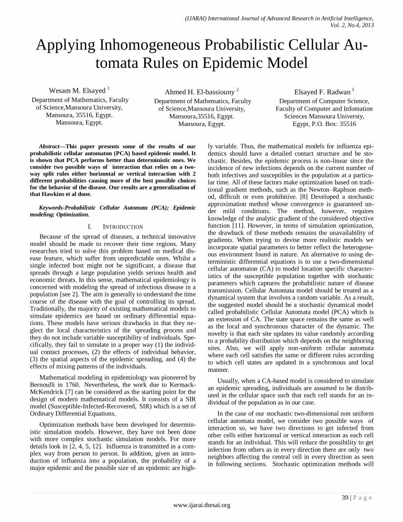
In this section, we describe the overall design of our au-tomaton. The model is a two-dimensional grid of cells, each cell containing the same or different rules due to the fact that each epidemic can be in any one of four stages as in the SEIR model we introduced later (i.e. Susceptible, Exposed, Infected and Recovered). The susceptible individuals are those capable of contracting the disease; For many infections there is a peri-od of time during which the individual has been infected but is not yet infectious himself; during this latent peiod the individ-ual is said to be exposed. In this case we have the SEIR model in which the new class of exposed individuals (E) must be considered. The infectious individuals are those capable of spreading the disease; and the recovered individuals are those immune from the disease, either died from the disase, or hav-ing recovered, are definitely immune to it. So, different diag-nosis of disease has different rules. The neighbors of any cell in the grid are the cell itself plus the four orthogonal adjacent cells (fig. 1) according to von Neumann.
Fig. 1. The two-dimensional cellular automata cell's neighbors
Once the automaton was embedded in the grid, the cell as an
individual finite state machine, began to follow the rule that is applied to it. A single cell cannot do much without interacting with other cells. The lattice starts out with an initial configuraion of cells in which the following hold.
Each cell can take on one of the 4 different states:
1) Susceptible (i.e. healthy; designated as 0)
2) Exposed (designated as 1)
3) Infected (designated as -1)
4) Recovered (includes both survivors and deaths; desig-
nated as 2)
It is supposed that the way of infection is the contact between the infected individual and the healthy indi-vidual.
Once the healthy individuals have contracted the infec-tion and have recovered from it, they acquire tempo-rary immunity.
B. Mathematical Formulation Of The PCA
Two-dimensional CA are discrete dynamical systems formed by a finite number of identical objects called cells, which are arranged uniformly in a two-dimensional space. Each cell is endowed with a state, belonging to a finite state set, that changes at every discrete step of time according to a rule, called local transition function. More precisely, a CA can be defined as a 4-uplet, A = (C, S, N, f), where C is the cellu-
lar space formed by a two-dimensional array of r × c cells
,where r stands for rows and c for columns (see Fig. 2-(a)): C
= {(a, b) , 1 ≤ a ≤ r, 1 ≤ b ≤ c}. The state of each cell is an ele-ment of a finite set, S, in such a way that the state of the cell
(a, b) at time t is denoted by StbaS ;, . The matrix
tjiStC ;,)( is called configuration of the CA at time t.
Moreover, )0(C is the
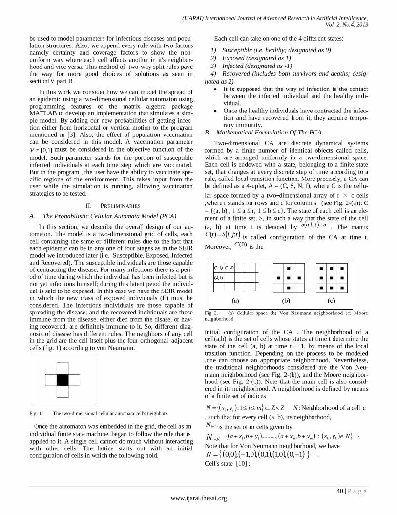
Fig. 2. (a) Cellular space (b) Von Neumann neighborhood (c) Moore
neighborhood
initial configuration of the CA . The neighborhood of a cell(a,b) is the set of cells whose states at time t determine the state of the cell (a, b) at time t + 1, by means of the local trasition function. Depending on the process to be modeled ,one can choose an appropriate neighborhood. Nevertheless, the traditional neighborhoods considered are the Von Neu-mann neighborhood (see Fig. 2-(b)), and the Moore neighbor-hood (see Fig. 2-(c)). Note that the main cell is also consid-ered in its neighborhood. A neighborhood is defined by means of a finite set of indices
c cell a of odNeighborho :1:, NmiyxN ii
, such that for every cell (a, b), its neighborhood,
N ba, is the set of m cells given by
Nyxybxaybxa kkmmbaN ,:,,,........., 11,
.
Note that for Von Neumann neighborhood, we have
1,0,0,1,1,0,0,1,0,0 N .
Cell's state [10] :
(IJARAI) International Journal of Advanced Research in Artificial Intelligence, Vol. 2, No.4, 2013
41 | P a g e www.ijarai.thesai.org
)1(2,1,10,1tSc
(2)1(t)c
S1)(tc
S:f
Where
1iteration at cell theof State: tSc function Transition:f (Determines how the cell’s state can
change). As the cellular space is considered to be finite, boundary
coditions must be taken into account in order to asure the well-defined dynamics of the CA.
C. Probabilistic Analysis of Cellular Automata Rules
With each time step, the state of each individual cell changes according to a set of rules based on the states of the cell’s neighbors. These rules can be either deterministic (cer-tain) or stochastic (probability-based/uncertain). To determine this exactly we need to define two essential factors, if the de-cision rules have the form C →D, meaning IF C THEN D, where C is the condition attribute, and D is the decision attrib-ute of the decision rule then we have ,
The certainty factor of the decision rule C →D, denoted by
),( DCcer , is defined as :
(3))/(),( CDpDCcer
Where ]1,0[),( DCcer . If 1),( DCcer , then the given
decision rule is a deterministic or certain decision rule .
Otherwise, 1),(0 DCcer , the given decision rule is a sto-
chastic or uncertain decision rule.
The coverage factor of the decision rule C →D in S, denoted
by ),cov( DC , is defined as:
(4))/(),cov( DCpDC
In this work we consider a non-uniform case of cellular a tomata where different cells may contain different rules. At a given moment, only one rule is active for a cell and deter-mines the cell's function. A non-active rules may be activated in next time steps.
Let any cell in the lattice be labeled by its position ji,c
where i and j are the row and column indices. A func-tion
tS c is the state of cell c at time step t . The rules of the
model specify how the state 1tS c is to be computed from
the states at time step t of it's neighbors
)1,(),1,(),,1(),,1( jijijijias in fig. 3:
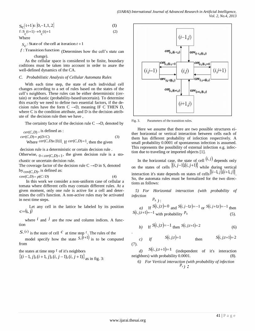
Fig. 3. Parameters of the transition rules.
Here we assume that there are two possible structures ei-ther horizontal or vertical interaction between cells each of them has different probability of infection respectively. A small probability 0.0001 of spontaneous infection is assumed. This represents the possibility of external infection e.g. infec-tion due to traveling or imported objects [1].
In the horizontal case, the state of cell ji, depends only
on the states of cells 1,,1, jiji
while during vertical
interaction it's state depends on states of cells jiji ,1,,1
. So, the automata rules must be formalized for the two direc-tions as follows:
5) For Horizontal interaction (with probability of
infection
hp
) :
a) If 0;, tjiS and 1;1, tjiS or 1;1, tjiS then 11;, tjiS with probability h
p (5).
b) If 1;, tjiS then 21;, tjiS (6)
.
c) If 1;, tjiS then 21;, tjiS
(7).
d) 11;, tjiS (independent of it's interaction
neighbors) with probability 0.0001. (8).
6) For Vertical interaction (with probability of infection v
p) :
(IJARAI) International Journal of Advanced Research in Artificial Intelligence, Vol. 2, No.4, 2013
42 | P a g e www.ijarai.thesai.org
a) If 0;, tjiS and 1;1, tjiS
or 1;1, tjiS
then 11;, tjiS with probability v
p (9).
b) If 1;, tjiS then 21;, tjiS (10).
c) If 1;, tjiS then 21;, tjiS (11).
d) 11;, tjiS (independent of it's interaction
neighbors) with probability 0.0001
(12).
If a cell is susceptible (0), the simulation module counts the number of infected cells that are its nearest neighbors. The simulation then calculates the probability the cell can avoid
being infected m1 ,where β is the infection rate (the probability a contact with an infected person is actually infectious) and m is the number of infected cells. Subtracting this value from 1 yields the probability of the cell being infected [10].
III. THE OPTIMIZATION PROBLEM
The optimization problem is as follows: Given a limited quantity of influenza vaccine and a particular population structure and infection rate pattern for a single wave of pandemic influenza, what proportion of each stage should be vaccinated to minimize the impact of the epidemic? [ see :9]
We divide the population into four different cases: Susceptible, Exposed , Infected and Recovered that are
indexed as 4,..,1i .We let ni be the number of individuals in
class i , and the total population size is
4
1i
inn
. We let be the infection rate, i.e. (the probability a contact with an
infected person is actually infectious), where either takes
the value hp or Vp
depending on the movement direction.
We let V be the total number of vaccine doses available be-
fore day one of the epidemic, and i the proportion of
individuals in case i that is vaccinated. Thus, the total number of doses distributed is,
13,
4
1
VQ
wherenQ i
i
i
since we cannot use more vaccine than there is available. We assume that each person vaccinated receives one dose of vaccine. Four different values of the vaccination rate are
considered: V = 0, 0.2, 0.3, 0.4. Note that as V increases, the number of infected individual decreases. To reflect the impact
of a single illness, we let iw be the weight assigned to an
illness in each case for minimization of the loss function. Then, the optimization problem is expressed as
144
1min iwin
i
Such that
154
1V
iiin
We concentrate on minimizing overall illness in the population as well as number of lives lost given a predeter-
mined number of doses V of vaccine. We use weights of one,
i.e. 4,...,1,1 iiw
for minimizing illness objective function. The rules have been applied based on an optimization algorithm as illustrated in Fig. 4 showing the behavior of the epidemic through different probabilities.
Pseudocode
Overall structure
Main function Get information from user and initialize variablesVisualise
state
Loop through generations:
1) Update count of infected neighbours for each cell
2) Update state of each cell based on number of infected
neighbours
3) Visualize state
4) Stop
In this work we consider how we can model the spread of an epidemic using a two-dimensional cellular automaton. We will use programming features of the matrix algebra package MATLAB to develop an implementation that simulates a sim-ple model [3] as shown in fig.4. We want to construct a model
of an epidemic that will develop over a fixed N by N grid in a given number of generations. We apply a set of rules to each cell that will determine its fate in the next generation, for ex-ample whether a given cell will become infected or not. The probabilities of state changes are a set of predefined parame-ters. By studying the effects of varying these parameters we try to predict how the epidemic will develop over time will it eventually die out.
We apply the same strategy of vaccination used by [3] where the user have the ability to vaccinate specific regions of the environment. This takes input from the user while the sim-ulation is running, allowing vaccination strategies to be tested. Since vaccination is not usually permanent but lasts for a pe-riod of time, it is implemented in much the same way as the temporary immunity that follows organism recovery. While the program is running, the user can click on the grid causing vaccination to be simulated at the clicked point.
(IJARAI) International Journal of Advanced Research in Artificial Intelligence, Vol. 2, No.4, 2013
43 | P a g e www.ijarai.thesai.org
Fig. 4. Pseudo code for main program
IV. SIMULATION AND ANALYSIS
A. Different scenarios based on varying p-horizontal ( hp)
and p-vertical ( vp)
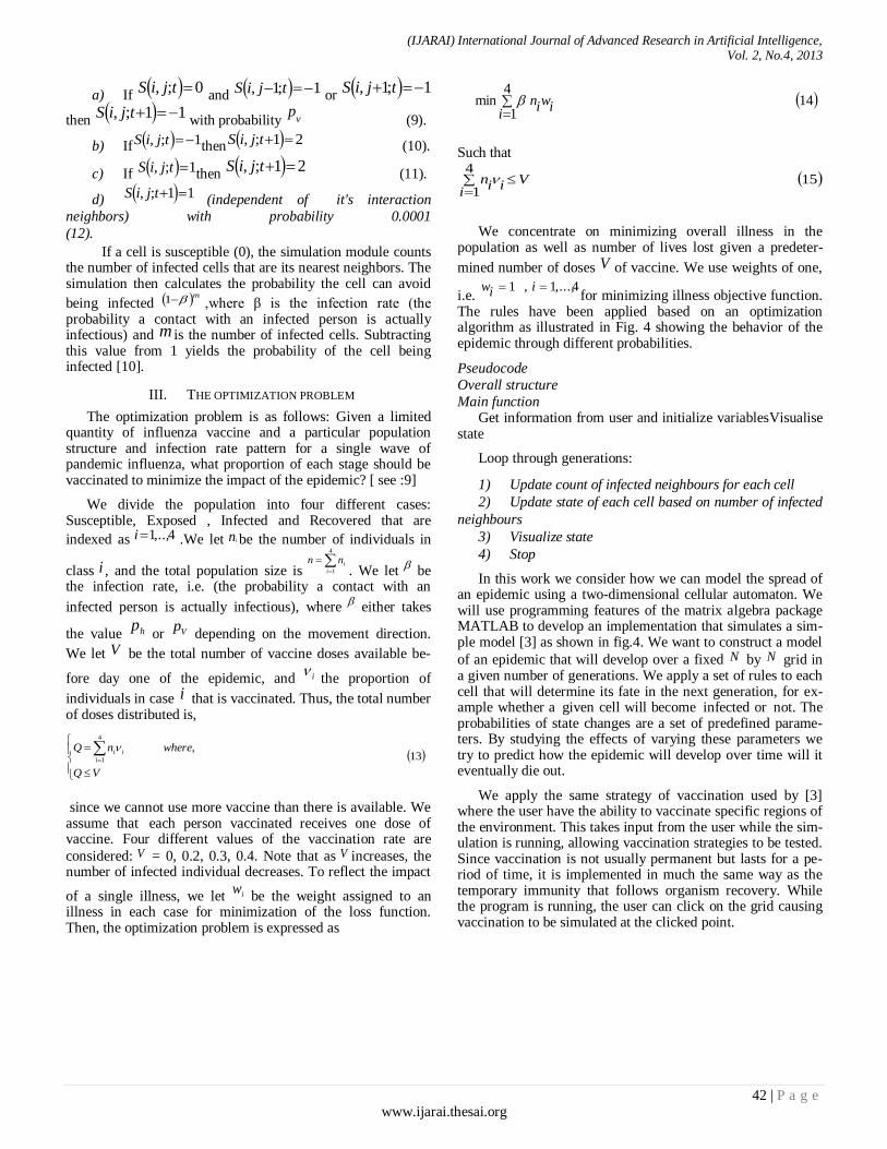
Because our cellular automaton is probabilistic (i.e. ran-dom numbers affect the chances of different scenarios arising,
even with fixed hp , vp
and q
) it is necessary to run several simulations to obtain an approximate understanding of what should happen to the spread of the epidemic. We also need to
test several different values of hp and vp
. Initially, we will
set q as a constant 1 and vary hp , vp
. Thus an Infected
cell will immediately become Recovered . We will test for hp , 9.0,7.0,5.0,3.0,1.0vp .
Case 1: .}9.0,7.0,5.0,3.0,1.0{,1.0 vh pp
Case2: .}7.0,5.0,3.0,1.0{,3.0 vh pp
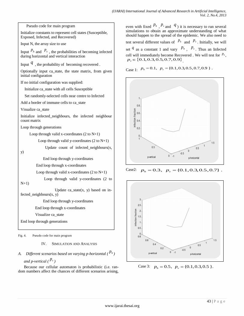
Case 3: .}5.0,3.0,1.0{,5.0 vh pp
Pseudo code for main program
Initialize constants to represent cell states (Susceptible, Exposed, Infected, and Recovered)
Input N, the array size to use
Input hp
and vp
, the probabilities of becoming infected during horizontal and vertical interaction
Input q
, the probability of becoming recovered .
Optionally input ca_state, the state matrix, from given initial configuration
If no initial configuration was supplied:
Initialize ca_state with all cells Susceptible
Set randomly-selected cells near centre to Infected
Add a border of immune cells to ca_state
Visualize ca_state
Initialize infected_neighbours, the infected neighbour count matrix
Loop through generations
Loop through valid x-coordinates (2 to N+1)
Loop through valid y-coordinates (2 to N+1)
Update count of infected_neighbours(x, y)
End loop through y-coordinates
End loop through x-coordinates
Loop through valid x-coordinates (2 to N+1)
Loop through valid y-coordinates (2 to N+1)
Update ca_state(x, y) based on in-fected_neighbours(x, y)
End loop through y-coordinates
End loop through x-coordinates
Visualize ca_state
End loop through generations
(IJARAI) International Journal of Advanced Research in Artificial Intelligence, Vol. 2, No.4, 2013
44 | P a g e www.ijarai.thesai.org
Case 4: .}3.0,1.0{,7.0 vh pp
B. We run the simulations for 100 generations and observe
the behavior of the disease in a grid of size 50 × 50 .
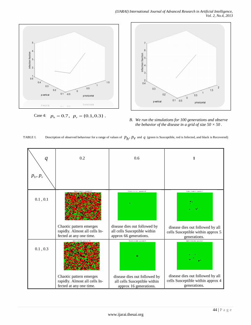
TABLE I. Description of observed behaviour for a range of values of vph
p , and q (green is Susceptible, red is Infected, and black is Recovered)
q
vh pp ,
0.2
0.6
1
0.1 , 0.1
Chaotic pattern emerges
rapidly. Almost all cells In-
fected at any one time.
disease dies out followed by
all cells Susceptible within
approx 66 generations.
disease dies out followed by all
cells Susceptible within approx 5
generations.
0.1 , 0.3
Chaotic pattern emerges
rapidly. Almost all cells In-
fected at any one time.
disease dies out followed by
all cells Susceptible within
approx 16 generations.
disease dies out followed by all
cells Susceptible within approx 4
generations.
(IJARAI) International Journal of Advanced Research in Artificial Intelligence, Vol. 2, No.4, 2013
45 | P a g e www.ijarai.thesai.org
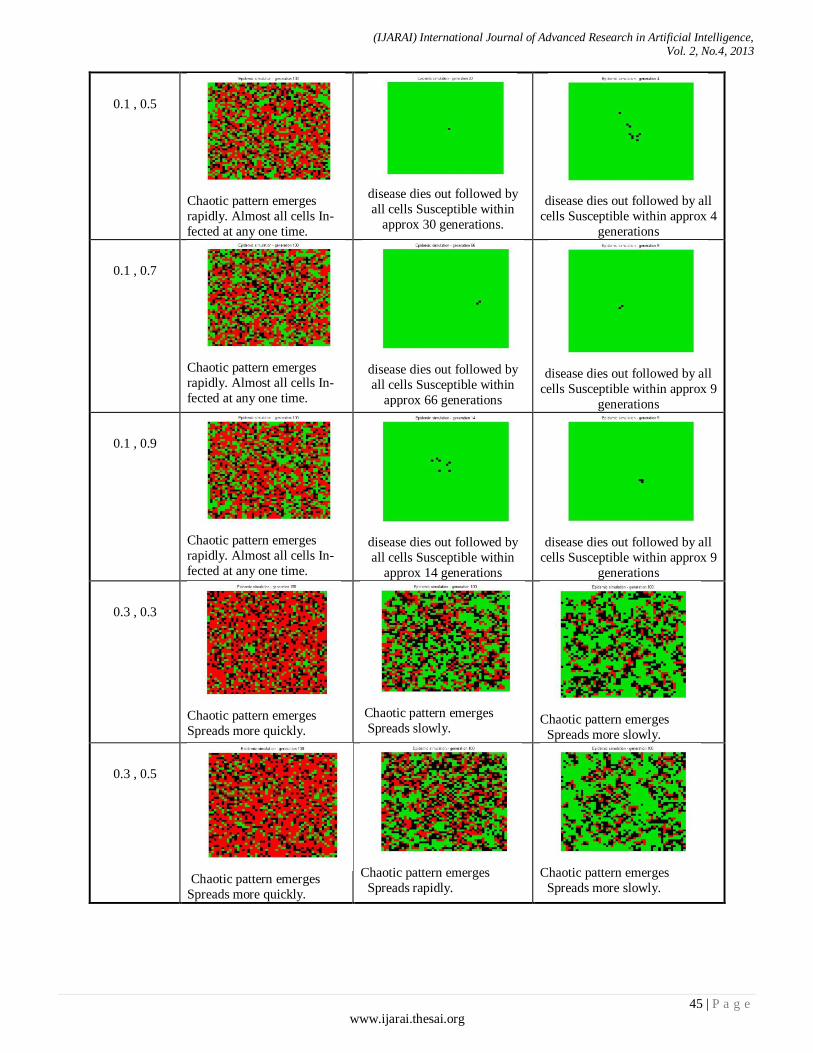
0.1 , 0.5
Chaotic pattern emerges
rapidly. Almost all cells In-
fected at any one time.
disease dies out followed by
all cells Susceptible within
approx 30 generations.
disease dies out followed by all
cells Susceptible within approx 4
generations
0.1 , 0.7
Chaotic pattern emerges
rapidly. Almost all cells In-
fected at any one time.
disease dies out followed by
all cells Susceptible within
approx 66 generations
disease dies out followed by all
cells Susceptible within approx 9
generations
0.1 , 0.9
Chaotic pattern emerges
rapidly. Almost all cells In-
fected at any one time.
disease dies out followed by
all cells Susceptible within
approx 14 generations
disease dies out followed by all
cells Susceptible within approx 9
generations
0.3 , 0.3
Chaotic pattern emerges
Spreads more quickly. Chaotic pattern emerges
Spreads slowly.
Chaotic pattern emerges
Spreads more slowly.
0.3 , 0.5
Chaotic pattern emerges
Spreads more quickly.
Chaotic pattern emerges
Spreads rapidly.
Chaotic pattern emerges
Spreads more slowly.

(IJARAI) International Journal of Advanced Research in Artificial Intelligence, Vol. 2, No.4, 2013
46 | P a g e www.ijarai.thesai.org
0.3 , 0.7
Chaotic pattern emerges
Spreads more quickly.
Chaotic pattern emerges
Spreads rapidly.
Chaotic pattern emerges Spreads more slowly.
0.5 , 0.5
Chaotic pattern emerges
Spreads more quickly.
Chaotic pattern emerges
Spreads rapidly.
Chaotic pattern emerges Spreads slowly.
Note that: the figures shown in table1 will be a bit different every time we execute the program as the vaccine is given ran-
domly by each user.
V. CONCLUSION
These epidemic scenarios presented above provide an op-portunity to demonstrate the visualization capabilities of a graphical CA model. When [3] use a single probability of in-fection, they got only two results in which all cells are in sus-ceptible state. But, here when dividing the cellular space into two directions of motion with two different probabilities of
infection, there are more optional values for vph
p , differ at
which generation it is obtained as shown above in table1. We introduced a theoretical model to simulate the spreading of an epidemic. It is based on transferring the problem into paramet-ric one and the rules into restrictions, obtaining the optimiza-tion problem (14). It is solved with the chosen values of
vph
p , and
q get the minimum value of the function which
minimize the impact of the epidemic.
VI. FUTURE WORK
PCA are lattice model of spatially extended systems with probabilistic local dynamical rules of evolution. It is difficult to analyze rigorously, so the computational simulation provide an alternative tool. So the future work is to develop an itera-tive Probabilistic Neural Networks with fully parallel proba-bilistic feedback dynamic. In addition, Parallel Genetic Algo-rithms can be incorporated by modifying the probabilities. PGA search through the space of parameters to calibrate the model to observe data. Whilst, PNN synthesis of approaches based on prior analysis and contextual information.
ACKNOWLEDGMENT We thank Prof. E. Ahmed, Mathematics Dept., Faculty of
Science, Mansoura University, Egypt, for his comments. Also,
special thanks for MATLAB Developers, where matrix alge-bra package is used for implementing that simulation model.
REFERENCES
[1] Ahmed E., Agiza H.N. , (1998) On modeling epidemics. Including latency, incubation and variable susceptibility, Physica A 253 347-352.
[2] Anderson, R., May, R., 1991. Infectious Diseases of Humans:Dynamics and Control. Oxford University Press, New York.
[3] Andrew Hawkins, Danny Roff, Adam Gundry, 2005. Cellular Automata
and Spatial Epidemics. November 25. http://citeseerx.ist.psu.edu/viewdoc/download?doi=10.1.1.105.1458&re
p=rep1&type=pdf.
[4] Greenhalgh, D., 1986. Control of an epidemic spreading in a heterogeneously mixing population. Math. Biosci. 80, 23–45.
[5] Hethcote, H., Waltman, P., 1973. Optimal vaccine schedules in
deterministic epidemic models. Math. Biosci. 18, 365–381.
[6] Hoya White S., Martı´n del Rey A., Rodrı´guez Sa´nchez G., (2007). Modeling epidemics using cellular automata. Applied Mathematics and
Computation 186 193–202.
[7] Kermack W.O., McKendrick A.G., Proc. Roy. Soc. Edin. (1927) A 115 700.
[8] Robbins, H., Munro, S., 1951. A stochastic approximation method. Ann. Math. Statist. 22, 400–407.
[9] Patel Rajan, Ira M. Longini Jr., M. Elizabeth Halloran,(2005) Finding
optimal vaccination strategies for pandemic influenza using genetic algorithms. Journal of Theoretical Biology 234. 201–212.
[10] Wang Jeffrey B., 2010. School’s Out? Designing Epidemic Containment
Strategies with a spatial stochastic method. http://www.dancingdarwin.com/sca.
[11] Weisstein, E., 2004. Robbins–munro stochastic
approximation.MathWorld;http://mathworld.wolfram.com/Robbins–MonroStochasticApproximation.html.
[12] Wickwire, K.H., Guest, D., 1976. Optimal control policies for reducing
the maximum source of a closed epidemic. Math. Biosci. 32, 1–14.
AUTHORS PROFILE
Wesam Elsayed, Department of Mathematics, Faculty of Science, Mansoura University, Mansoura, 35516, Egypt
(IJARAI) International Journal of Advanced Research in Artificial Intelligence, Vol. 2, No.4, 2013
47 | P a g e www.ijarai.thesai.org
E-mail address: [email protected]
Ahmed El-bassiouny , received his B.Sc. and M.Sc. from Mathematics Dept. Faculty of Science, Mansoura Uni-versity, Egypt. He received his Ph.D. from University of Kiev, Soviet Union. He became a Lecturer at Mathematics Dept., Faculty of Science, Mansoura University, Egypt on
2004.
E-mail address: [email protected]
Elsayed Radwan, received his B.Sc. and M.Sc. from Mathematics Dept. Faculty of Science, Mansoura University, Egypt. He received his Ph.D. from Intelligent Lab., Graduate School of Engineering, Toin University of Yokohama, Japan. He became a Lecturer at Computer Science Dept., Faculty of
Computer and Information Sciences, Mansoura University, Egypt on 2007. His areas of interest are Soft Computing, Evolutionary Computing, Pattern Recognition, and Cellular Neural Networks.
E-mail address: [email protected]


![Lectures on PROBABILISTIC LOGICS AND THE ......2 Probabilistic Logics 2. A SCHEMATIC VIEW OF AUTOMATA 2.1 Logics and Automata It has been pointed out by A. M. Turing [5] in 1937 and](https://img.pdfslide.us/doc/110x75/60b6c69776042e345216d9fd/lectures-on-probabilistic-logics-and-the-2-probabilistic-logics-2-a-schematic.jpg)

![Probabilistic Model Checkingqav.comlab.ox.ac.uk/papers/pmc-handbook.pdf · Markov decision processes [98, 86, 39], which are similar to probabilistic automata [100, 101], are a convenient](https://img.pdfslide.us/doc/110x75/5ed07c55af35d71fd24364cc/probabilistic-model-markov-decision-processes-98-86-39-which-are-similar-to.jpg)