Embed Size (px)
Citation preview
Applying DTGolog to Large-scale Domains
by
Huy N Pham
A thesis
presented to Ryerson University
in partial fulfillment of the
requirements for the degree of
Masters of Applied Science
in the Program of
Electrical and Computer Engineering
Toronto, Ontario, Canada, 2006
© Huy Pham 2006
ii
I hereby declare that I am the sole author of this thesis.
I authorize Ryerson University to lend this thesis to other
institutions or individuals for the purpose of scholarly research.
----------------------------------------
Huy Pham
I further authorize Ryerson University to reproduce this thesis
by photocopying or by other means, in total or in part, at the request of other
institutions or individuals for the purpose of scholarly research.
----------------------------------------
Huy Pham
iii
Abstract
While decision theoretic planning (DTP) offers great potential benefits to elicit
purposeful behavior of the agent operating in uncertain environments, state-based
approaches to DTP are known to be computationally intractable in large-scale domains.
DTGolog is a decision-theoretic extension of a logic-based high level programming
language Golog that completes a given partial Golog program using a form of directed
value iteration. DTGolog has been proposed to alleviate some of the computational
difficulties associated with DTP. The main advantages of DTGolog are that a DTP
problem can be formulated using a logical representation to avoid explicit state
enumeration, and the programmer can encode domain-specific knowledge in terms of
high-level procedural templates to partially specify behavior of an agent. These templates
constrain the search space to manageable size. Despite these clear advantages, there are
few studies that investigate the applicability of DTGolog to very large-scale practical
domains. In this thesis, we conduct two studies. First, we apply DTGolog to the well-
known case-study of the London Ambulance Service to demonstrate advantages and
potentials of DTGolog as a quantitative evaluation tool for designing decision making
agents. Second, we develop a software interface that allows to control the well-known
Sony's AIBO robotics platform using DTGolog. We show that DTGolog can be used on
this platform with a minimal amount of software customization. We run experiments to
test functionality of our interface. The main contribution of this thesis is demonstration of
applicability of DTGolog to two different large scale domains that are both practical and
interesting.

iv
Acknowledgements
I would like to thank my supervisor, Dr. Mikhail Soutchanski for his guidance and
support during the past two years.
I would like to thank Dr. Alagan Anpalagan, Dr. Alireza Sadeghian and Dr. Eric Harley
for reviewing my thesis and serving on my thesis committee.
I would like to thank Dr. John Mylopoulos for his inspiration and guidance during a
course project upon which the work reported in chapter 3 of this thesis was based.
v
Table of Contents
1 Introduction....................................................................................................1
2 Background....................................................................................................6
2.1 Markov Decision Process ....................................................................................6
2.2 Situation Calculus..............................................................................................10
2.2.1 Actions .......................................................................................................11
2.2.2 Situation .....................................................................................................13
2.2.3 Fluents........................................................................................................13
2.2.4 Action Theory ............................................................................................14
2.2.5 Optimization Theory..................................................................................15
2.3 Golog and DTGolog...........................................................................................16
2.3.1 Control Structures ......................................................................................17
2.3.2 Evaluation Semantics.................................................................................19
2.3.3 Procedural Interpretation ...........................................................................27
2.3.4 On-line DTGolog Interpreter .....................................................................28
2.4 Alternatives to DTGolog ...................................................................................29
3 A DTGolog-based Resource Allocator for the London Ambulance Service ...............................................................................................................32
3.1 Introduction and Motivation ............................................................................32
3.2 The London Ambulance Service (LAS)...........................................................33
3.3 Domain Representation.....................................................................................35
3.3.1 Simple Domain Characteristics..................................................................39
vi
3.3.2 More Complex Domain Characteristics.....................................................40
3.4 Resource Allocator Design................................................................................45
3.4.1 The Manual Design....................................................................................45
3.4.2 The Automated Design ..............................................................................48
3.4.3 The Optimized Design ...............................................................................51
3.4.4 Other designs .............................................................................................53
3.5 Simulation Results .............................................................................................54
4 Controlling the Sony AIBO robot ..............................................................61
4.1 Introduction .......................................................................................................61
4.1.1 The Sony AIBO Robot...............................................................................61
4.1.2 Some well-known AIBO-based research projects .....................................63
4.1.3 Some potential benefits of interfacing Golog to Tekkotsu ........................64
4.2 A Golog-Tekkotsu Interface .............................................................................66
4.2.1 Software Architecture ................................................................................66
4.2.2 Operations ..................................................................................................67
4.2.3 Exported API .............................................................................................68
4.3 A test case ...........................................................................................................68
4.3.1 A Navigation Task .....................................................................................68
4.3.2 Possible approaches ...................................................................................69
4.3.3 Doing hierarchical reasoning in Online DTGolog.....................................72
4.3.4 Domain Representation..............................................................................75
4.3.5 Control Procedures.....................................................................................81
4.3.6 Results........................................................................................................86
5 Conclusion...................................................................................................87

vii
5.1 Summary ............................................................................................................87
5.2 Contributions .....................................................................................................88
5.3 Future Works.....................................................................................................88
viii
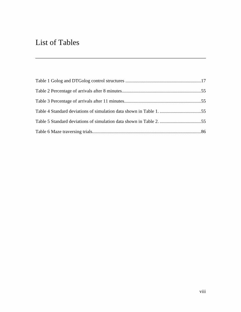
List of Tables
Table 1 Golog and DTGolog control structures ................................................................17
Table 2 Percentage of arrivals after 8 minutes...................................................................55
Table 3 Percentage of arrivals after 11 minutes.................................................................55
Table 4 Standard deviations of simulation data shown in Table 1. ...................................55
Table 5 Standard deviations of simulation data shown in Table 2. ...................................55
Table 6 Maze traversing trials............................................................................................86
ix
List of Figures
Figure 1 Agent-Environment Interaction.............................................................................6
Figure 2 A fixed depth look-ahead tree .............................................................................28
Figure 3 Possible scenarios of an emergency service trip .................................................34
Figure 4 The three LAS regions as represented by 3 rectangular grid worlds ..................36
Figure 5 Overall organization of the project......................................................................38
Figure 6 Percentage of arrivals after 8 minutes graph. ......................................................56
Figure 7 Percentage of arrivals after 11 minutes graph. ....................................................56
Figure 8 Standard deviations for the 8 minutes simulation data........................................57
Figure 9 Standard deviations for the 11 minutes simulation data......................................57
Figure 10 The Sony Aibo as an entertainment robot .........................................................62
Figure 11 Abstraction Layers of Robotics applications.....................................................65
Figure 12 Software Architecture of the interface ..............................................................67
Figure 13 A navigation problem........................................................................................68
Figure 14 A 3x3 Grid world representing the maze ..........................................................76
x
List of Appendixes
Appendix A .............................................................................................................A1
Appendix B .............................................................................................................B1
Appendix C .............................................................................................................C1
Appendix D .............................................................................................................D1
1
1 Introduction
Decision theoretic planning offers great potential benefits in the fields of AI and
Robotics. Given the complete and accurate model of the world’s dynamics, decision
theoretic planning provides a decision making agent not only with the ability to figure out
a way to accomplish its goals but also with the ability to accomplish these goals in an
optimal way. In the ideal situation where decision theoretic planning can be used, many
difficult control and programming problems can be reduced to the task of representing
these problems in a fully observable Markov Decision Process (MDP) model, because a
decision theoretic DT planner would figure out all remaining details on its own.
Unfortunately, decision theoretic planning has always been a computationally
challenging task. Real-world and complex domains often involve hundreds of different
state features and hundreds, possibly thousands, of actions. Because the number of states
growth exponentially with the number of state features (Bellman’s “curse of
dimensionality”), traditional state-based approaches to planning, which require explicit
enumeration of states, are known to be intractable for most if not all these cases.
To cope with this problem, some advanced decision theoretic planning frameworks have
been proposed. Decision Theoretic Golog (DTGolog) is one of such frameworks. With an
origin in the field of Knowledge Representation, DTGolog avoids the computational
problems associated with traditional state-based approach by representing the decision
theoretic planning problem using a logical representation and avoiding explicit
enumeration of states. Also, it embraces the idea of partial programming by allowing the
2
agent programmer to encode domain-specific knowledge into expressive1 high-level
procedural templates that partially specify the behavior of the agent and constrain its
search space to a manageable size. Given as input a high-level procedural template that
might contain non-deterministic choices between actions, the DTGolog interpreter builds
and searches a fixed-depth look-ahead decision tree that is rooted at the current state and
contains all the possible actions specified by the input template, to produce a fully
specified program that is optimal with respects to the set of possible programs specified
by the input template. Taking this approach (which is called directed value iteration in
MDP literature) to decision theoretic planning, DTGolog has a computational advantage
because computation is focused to just the states and actions that are reachable from the
current state. Also, because of the expressiveness offered by the framework, DTGolog
programmers have a fine-grain control over the degree of planning vs. programming that
can remain in a template because they have the ability to decide what amount of available
domain-specific knowledge can be used. As a consequence, optimality and tractability
can be finely traded for each other in this framework.
Given the above mentioned theoretical advantages and potentials offered by the DTGolog
framework, the degree of popularity that it has gained, especially from outside of the
logic-based communities, is still limited. This is due, partially, to the fact that there have
been a limited number of real-world applications to which this framework has been
applied, and the fact that there are still a very limited number of real and interesting
robotics platforms on which DTGolog can be used with a minimal amount of software
customization. Previously, DTGolog has been applied to a realistic office delivery
problem with a mobile robot and also to a factory processing domain [24]. It has also
been applied to control mobile robots playing robotic soccer [10;11], and to personalize
Web services [12]. To advocate the usefulness and practicality of the DTGolog
1 Because it is based on the language of first-order logic, DTGolog has the expressiveness of that language.
3
framework, this thesis aims to further this list of DTGolog’s successful applications, and
has two main objectives:
(1) To apply DTGolog to a very large scale domain to demonstrate its advantages
and potentials. More specifically, we want to apply the framework of DTGolog
to the domain of the London Ambulance Service to demonstrate its advantages
and potentials as a quantitative tool for evaluating and comparing different
designs of decision making agents, one of the most essential tasks in software
engineering. The London Ambulance Service (LAS) problem comes from an
investigation into a failed attempt to computerize the LAS and has become a
well-know case-study in the field of software and requirement engineering.
Because of its complexity and challenging characteristics, this case study has
become almost a benchmark domain for requirement engineering methodologies,
and several researchers have used this case study to demonstrate their
frameworks. Most of the proposed frameworks, however, rely on qualitative
methods and lack the capability to provide a quantitative evaluation for different
designs. The objective of this work is to demonstrate DTGolog’s advantages and
capabilities as a quantitative designs evaluation tool.
(2) To create a complete DTGolog-based high-level cognitive robotics platform that
can be used for both research and education purposes by developing a software
interface that would allow DTGolog to be used on a real and interesting robotics
platform. More specifically, we want to develop a software interface that would
bridges DTGolog with the Tekkotsu framework, a software development
framework developed and maintained at Carnegie-Mellon University for the
commercially available Sony’s Aibo robot, that would allows (DT)Golog
programs to control the Sony ERS7 robot. Intended to be used as a high-level
agent programming language, DTGolog provides the agent programmer with
everything he needs to (partially) specify the agent’s high-level behavior. Most
robot control tasks however, require the programmer to specify not only the
4
high-level behavior but also the lower-level behaviors such as perception,
kinematics, etc... These low-level control tasks are usually very time consuming
and, for researchers who just want to focus on the decision making aspect of
robotics, can be a big, sometime prohibitive, burden. To foster the use of
DTGolog as a high-level robot programming tool, these burdens need to be
minimized. The objective of this work is to create a complete DTGolog-based
platform that can be used by researchers who want to test their ideas about high-
level decision making on a real robotics platform without the usual overhead of
manually integrating or programming all the lower-level building blocks.
The primary research methodology used in this thesis is experimental methods, and the
verification method is repeated test runs of programs.
The thesis is organized as follows. Chapter 2 reviews all the background materials that
are needed for the discussions that follow in the later parts of the thesis. In this chapter,
the framework of Markov Decision Process is first introduced as the theoretical basis for
probabilistic optimal decision making and decision theoretic planning. Then, the
language of Situation Calculus and high-level programming languages, Golog and
DTGolog, are introduced as logic-based planning and decision theoretic planning tools.
Chapter 3 reports the work we did to demonstrate DTGolog’s practicality and
applicability on large-scale domains. In this chapter, the London Ambulance Service’s
dispatching problem is first described and motivated. Then, a detail formulation of the
problem is given, followed by a complete description of the domain’s logical
axiomatization. Subsequently, we discuss alternative dispatching strategies and provide
simulation results. Chapter 4 describes the software interface that we developed, together
with a small but real and illustrative robotics application that demonstrates how the
interface can be used, as well as a new and convenient way of doing hierarchical
reasoning in the online version of DTGolog. In this chapter, the Sony AIBO robot,
together with its related well-known research projects, are first introduced. Some
motivations for a software interface between DTGolog and AIBO’s Tekkotsu

5
development framework is also given. Then, the architecture, operation, and API of the
interface are described. Finally, a complete description and axiomatization of the
demonstration problem is given. Chapter 5 discusses some future research directions.
6
2 Background
2.1 Markov Decision Process
Markov Decision Process (MDP) is a mathematical framework that can be used for
modeling decision-making in situations where outcomes are partly random and partly
under the control of the decision maker.
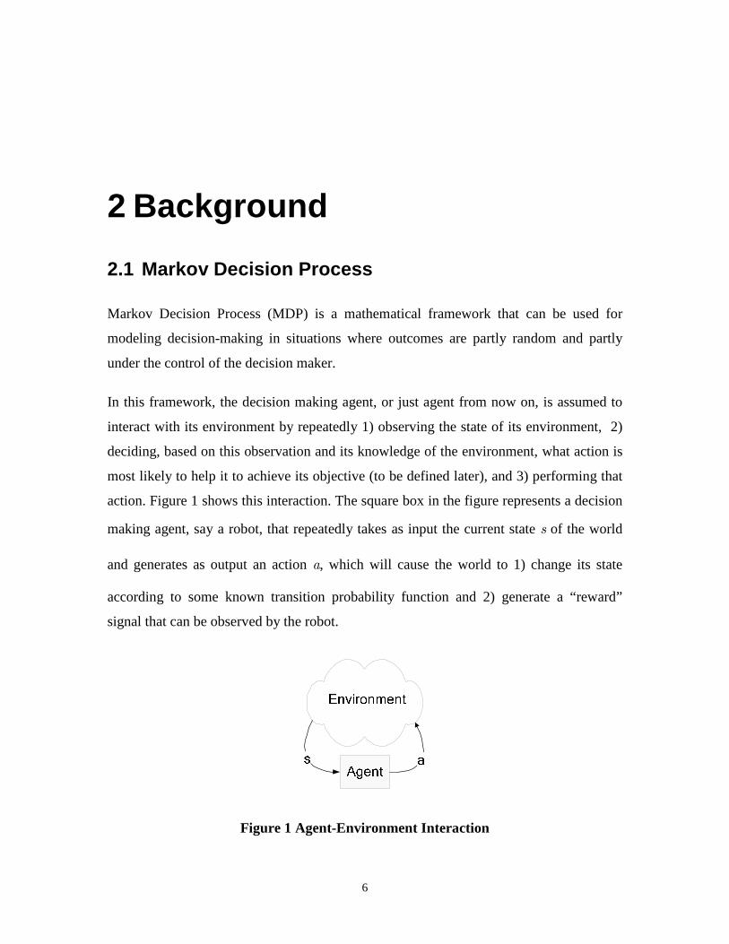
In this framework, the decision making agent, or just agent from now on, is assumed to
interact with its environment by repeatedly 1) observing the state of its environment, 2)
deciding, based on this observation and its knowledge of the environment, what action is
most likely to help it to achieve its objective (to be defined later), and 3) performing that
action. Figure 1 shows this interaction. The square box in the figure represents a decision
making agent, say a robot, that repeatedly takes as input the current state s of the world
and generates as output an action a, which will cause the world to 1) change its state
according to some known transition probability function and 2) generate a “reward”
signal that can be observed by the robot.
Figure 1 Agent-Environment Interaction
7
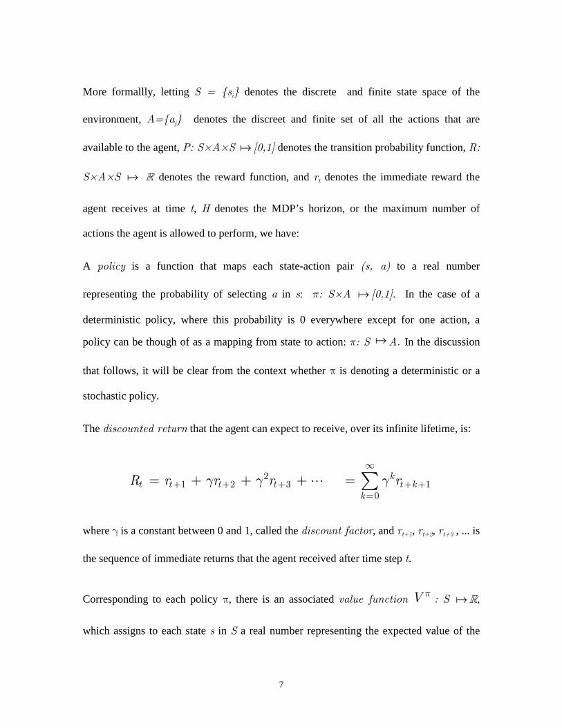
More formallly, letting S = {si} denotes the discrete and finite state space of the
environment, A={aj} denotes the discreet and finite set of all the actions that are
available to the agent, P: S×A×S ֏ [0,1] denotes the transition probability function, R:
S×A×S ֏ R denotes the reward function, and rt denotes the immediate reward the
agent receives at time t, H denotes the MDP’s horizon, or the maximum number of
actions the agent is allowed to perform, we have:
A policy is a function that maps each state-action pair (s, a) to a real number
representing the probability of selecting a in s: π: S×A ֏ [0,1]. In the case of a
deterministic policy, where this probability is 0 everywhere except for one action, a
policy can be though of as a mapping from state to action: π: S ֏A. In the discussion
that follows, it will be clear from the context whether π is denoting a deterministic or a
stochastic policy.
The discounted return that the agent can expect to receive, over its infinite lifetime, is:
21 2 3 1
0
kt t t t t k
k
R r r r rγ γ γ
∞
+ + + + +=
= + + + = ∑⋯
where γ is a constant between 0 and 1, called the discount factor, and rt+1, rt+2, rt+3 , ... is
the sequence of immediate returns that the agent received after time step t.
Corresponding to each policy π, there is an associated value function V π : S ֏R,
which assigns to each state s in S a real number representing the expected value of the
8
discounted total reward Rt that the robot will receive, if it starts from s and follows π
(that is, always selects the action π(s) in every state s ∈ S ) thereafter:
' ''
( ) [ | ]
( , ) [ ( ')]
t t
a ass ss
a s
V s E R s s
s a P R V s
π
ππ γ
= =
= +∑ ∑
where 'a
ssP is a shorthand for P(s, a, s’) and 'assR is a shorthand for R(s, a, s’). Similarly,
there is an associated action-value function Qπ: S ×A ֏R, which assigns to each
state-action pair (s, a) a real number representing the expected value of the discounted
total reward Rt that the robot would receive, if it starts from s, performs action a, and
then follows π thereafter:
' '' '
( , ) [ | , ]
[ ( ', ') ( ', ')]
t t t
a ass ss
s a
Q s a E R s s a a
P R s a Q s a
π
πγ π
= = =
= +∑ ∑
A policy that maximizes the value function is called an optimal policy, and its
corresponding value function is called the optimal value function, which is unique and is
shared by all the optimal policies, if more than one exists. The following equations,
called the Bellman optimality equations, characterize the optimal value of a state (or
state-action pair) in terms of the optimal values of its possible successor states (or state-
action pair)
9
* *' '
'
* *' '
''
( ) [ ( ')]
( , ) [ { ( ', ')}]
a ass ss
as
a ass ss
as
V s max P R V s
Q s a P R max Q s a
γ
γ
= +
= +
∑
∑
and can be used to determine the optimal value function.
One of the most well-known and fundamental method for finding the optimal value
function, as well as an associated optimal policy, is a dynamic programming algorithm
called Policy Iteration. This algorithm alternates between two phases: a Policy Evaluation
phase, in which it updates the value function associated with the current policy, and a
Policy Improvement phase, in which it derives a new and better policy from the current
value function. During the policy evaluation phase, Policy Iteration algorithm sweeps
through the state space and uses Bellman’s equation to update each state’s current
estimate base on the old estimates of its successor states:
' ' 1'
( ) ( , ) [ ( ')]a ak ss ss k
a s
V s s a P R V sπ γ −← +∑ ∑
where Vk(s) is the new estimated value of for s, and Vk-1(s’) is the old estimated value for
the successor s’ of s. The sweeping process is repeated until the current estimates of all
states converge to a predefined acceptable error. During the policy improvement phase,
the algorithm uses the current value function to update the policy:
' ''
( ) [ ( ')]a ass ss
a s
argmaxs P R V sπ γ = + ∑
One important special case of the Policy Iteration algorithm is another dynamic
programming algorithm called Value Iteration. Instead of doing policy evaluation until
the estimated values of all states converge, Value Iteration performs only one sweep per
10
policy evaluation phase. Bellman has shown in his 1957 book that if all states are updated
infinitely often, this sequence of estimated state values for all states will converge to the
real optimal value function.
In the case of finite horizons, the two Bellman Optimality Equations above can be
rewritten as:
* *' ' 1
'
* *' ' 1
''
( ) [ ( ')]
( , ) [ { ( ', ')}]
a an ss ss n
as
a an ss ss n
as
V s max P R V s
Q s a P R max Q s a
γ
γ
−
−
= +
= +
∑
∑
Using these equations, one can compute in sequence the optimal state value functions up
to the horizon H of interest. To compute this, Value Iteration algorithm would take H
iterations. At each iteration, it does |A| computations of |S|×|S| matrix times |S|-vector.
Thus, in total it requires O(H×|A|×|S|3) operations. Because the number of states grows
exponentially with the number of features used to represent the states, and because value
iteration works on the set of all policies, which can be very large, value iteration becomes
impractical once the number of features becomes large.
To address this problem, several techniques and frameworks that use compact
representations [3;4;19] have been proposed. Decision Theoretic Golog (DTGolog),
described in the next few sections, is one of such a framework. In contrast to value
iteration, DTGolog avoids explicit enumeration of states and focuses on a much smaller
subset of policies: those policies that satisfy constraints imposed by a Golog program.
2.2 Situation Calculus
The language of the situation calculus (SC) is a (second-order) logical language that was
first introduced by John McCarthy [15] as a vehicle for axiomatizing dynamically
11
changing worlds, and has been considerably extended in the 1990s to allow the modeling
of, and reasoning about, concurrency, continuous time, non-determinism, etc.
There are three fundamental concepts in the SC language [18]: actions, situations, and
fluents, each plays a different role. This section reviews these concepts and the different
classes of SC axioms that are used in specifying dynamic worlds. Emphasis in this
section is placed on the decision theoretic extension of the situation calculus.
2.2.1 Actions
Actions are represented in the framework of SC by terms (function symbols or constants).
In the temporal SC considered here, all action terms have at least one argument and this
argument (it is always the last argument) is the time when action occurs.
As an example, consider a world in which a robot has five fair coins that it can toss, one
by one. Once all the coins have been tossed, the robot can pick them up, and the trial
ends. To represent these actions, one would use:
toss(c, t): Toss the coin c at time t
pickup(t): Pickup all the coins at time t
It can be noted that these two actions are different in nature. Tossing a coin is a
stochastic, or nondeterministic, action because it has two possible different outcomes,
either heads or tails. Picking the coins up, on the other hand, is a deterministic action,
because it has only one outcome, all coins picked up.
To specify an action as deterministic, we use the predicate
deterministic(a, s)
where a is the action, s is a situation, to be described later, in which a is performed. For
example, to express the fact that pickup() is a deterministic agent action, we would write:
12
deterministic(pickup(t), s)
To specify an action as stochastic, that is, it has more than one possible outcome, the
following axiom is used:
nondetAction(a, outcomes, s)
where a is the action, outcomes is the list of possible outcomes, which are thought of as
nature’s actions (as opposed to agent action), and s is the situation in which a is to be
performed. For example, the stochastic nature of toss() can be expressed as:
notdetActions(toss(c, t), [tossHead(c, t), tossTail(c,t)], s)
which states that if the agent action toss() is performed in the situation s, the outcome
will be one of tossHead() and tossTail(), which are considered to be nature’s actions
that happen beyond the control of the agent.
To specify the probability associated with each outcome, or nature action, the following
axiom is used:
prob(n, p, s)
where n is the nature action, p is the probability that nature action n happens in situation
s. For example, assumming that all the coins are fair coins, the probabilities of the
outcomes of toss() can be expressed as follows:
prob(tossHead(c, t), 0.5, s)
13
prob(tossTail(c, t), 0.5, s)
which state that the chance of coming up head or tail is 0.5 in all situtations.
2.2.2 Situation
A situation represents a possible history of the world, and is a first order term constructed
from a finite sequence of actions, either an agent’s deterministic actions or nature’s
actions, using a special function symbol do(⋅,⋅). For example, the situation
do(tossHead(3, 5), do(tossTail(1, 4), do(tossTail(2, 1), S0)))
where S0 is a special constant symbol used to represent the initial situation (when the
world is thought to begin), is a situation denoting the history resulting after the agent has
tried to toss the second, first, and third coin, in that order, and it happened that the third
coin turned up head, while the other two turned up tail.
2.2.3 Fluents
Relations and functions in a dynamic world typically change their values from one
situation to the next. Such relations and functions are called fluents, and are represented
by relation and function symbols that take a situation term as their last argument. For
example, in the coin example above, one would have two relational fluents called
head(c, s) and tail(c, s) to denote whether the coin c is turning its head or tail up in the
situation s, and a relational fluent called tossed(c, s) to denote whether the agent has
previously tossed the coin c in the situation s.
14
2.2.4 Action Theory
Once all the agent actions, and their outcomes (or nature’s actions) have been specified,
the following set of axioms will be needed in order to do logical reasoning
2.2.4.1 Precondition Axioms
For each deterministic agent action and each nature’s action, one precondition axiom is
needed. A precondition axiom of an action is a logical statement of the form
Poss(a(x�
), s) ≡ ϕ(s)
where Poss is a special predicate symbol denoting whether it is possible for the action
a(x�
) to be executed in the situation s (a(x� ) is either an agent’s deterministic action or
nature’s actions), and ϕ is a SC uniform formula (that is, a formula that does not contain
the predicate constants Poss and the term do, mentions only one situation variable s and
it does not include quantifiers over this situation variable). For example, to express the
fact that it is always possible for a coin to turn up head, one would write
Poss(tossHead(c, t), s) ≡ True
Or, to express that it is possible to pick up all the coins if and only if the robot has tossed
all of them:
Poss(pickup(t), s) ≡ tossed(1, s)∧tossed(2, s)∧ ... ∧tossed(5,s)
2.2.4.2 Successor State Axioms and Initial Situation
For each fluent defined in the domain, one successor state axiom is needed. A successor
state axiom of a fluent completely specifies how the value of that fluent would change
when an action a is performed, and has the following form
15
F(x�
, do(a,s)) ≡ ΠF(x�
, a, s) ∨ [ F(x�
, s) ∧ ¬ ΝF( x�
, a, s) ]
where F is the fluent symbol, ΠF is a uniform formula representing the positive effect
condition for F (what makes it true) and ΝF is a uniform formula representing the
negative effect condition for F (what makes it false). For example, to specify how the
fluents head(c, s) and tossed(c, s) would change, one would write:
head(c, do(a,s)) ≡ a = tossHead(c, t) ∨ ¬ a = tossTail(c, t) ∧ head(c, s)
toss(c, do(a,s)) ≡ a = tossHead(c, t) ∨ ¬ a = putDown(x) ∧ holding(x, s)
2.2.4.3 Unique Naming Axioms
In addition to the precondition and successor state axioms described above, an action
theory also includes a set of sentences that say all the actions are pair wise unequal (and
all constants mentioned in the theory are not equal to make sure that they have distinct
interpretations).
2.2.5 Optimization Theory
A decision-theoretic optimization theory contains axioms that specify the reward function
and the actual outcome (of stochastic agent actions) which can be sensed. Axioms
specifying probabilities of outcomes corresponding to transition probabilities in MDP,
are usually also included in the optimization theory.
2.2.5.1 Axioms for Reward Function
Reward function is specified by an axiom of the form
reward(r, do(a,s)) def
= φ1(s) ∧ r=r1 ∨ ... ∨ φk(s) ∧ r=rk
16
which states that if the agents gets from the situation s into the situation do(a, s), it will
receive a reward r equals to one of the ri, depending on what was true in s.
2.2.5.2 Outcome probabilities axioms
For each possible outcome (i.e., nature action) of a stochastic agent’s action, there is one
axiom of the form
prob(n, p, s) def
= φ1(s) ∧ p=p1 ∨ ... ∨ φk(s) ∧ p=pk
which states that the probability p of nature action n happening in s is equals to one of the
pi, depending on what was true in s.
2.2.5.3 Outcome sensing axioms
In order to be able to determine which nature action has actually occurred after
performing a stochastic action, the agent needs to be provided with an axiom of the form:
senseCond(n, φ) def
= φ=φ1 ∧ n=n1 ∨ ... ∨ φ=φk ∧ n=nk
which states that nature action ni has actually occurred if φi (which is a situation
suppressed logical expressions) evaluates to true against the situation resulted from
performing a stochastic action.
2.3 Golog and DTGolog
Planning in Computer Science has always been very desirable but difficult to achieve. In
agent programming in particular, decision theoretic would provide agents with the ability
to figure out, given the complete and accurate model of the world’s dynamics, the
optimal behavior, i.e., the best sequence of actions. Unfortunately, complex domains are
17
often characterized by hundreds of different state features (or fluents in the context of
SC), and may involve hundreds, or possibly thousands of actions, and planning is known
to be computationally intractable in most if not all those cases.
Golog, and its decision theoretic extension, DTGolog, in particular, are situation
calculus-based planning, or decision theoretic planning in the case of DTGolog, tools that
were designed to be used as high-level agent programming languages in which optimality
is given up for tractability.
2.3.1 Control Structures
The standard control structures that can be found in Golog and DTGolog are summarized
below.
Table 1 Golog and DTGolog control structures
Syntax Meaning
δ1 ; δ2 Program expression δ1 must be executed before program
expression δ2
φ? Test the truth value of logical expression φ in the current
situation
δ1 | δ2 Either program expression δ1 or δ2, which ever is better, should
be executed
18
π(x : τ) δ(x)
Program expression δ, of which x is an argument, should be
executed with the best argument from the finite set τ substituted
for x
(π x)δ(x) Program expression δ should be executed with any valid
argument.
if φ then δ1 else δ2 Program expression δ1 should be executed if φ is true in the
current situation, otherwise, δ2
while φ do δ Program expression δ should be done as long as φ is true
proc(p, δ) Program expression δ can be executed by calling procedure p
local(δ1);δ
First, compute the optimal policy π1 corresponding to the sub-
program δ1, then compute the optimal policy π corresponding to
the program π1;δ
limit(δ1);δ
Without looking into δ, compute the optimal policy π1
corresponding to the subprogram δ1, execute it to completion,
and then compute and execute the policy π corresponding to δ.
19
2.3.2 Evaluation Semantics
This section describes the semantics of the DTGolog constructs (i.e., program operators)
listed above. Everywhere in this section we have in mind only finite horizon MDPS.
First, a policy in the context of Golog is a deterministic (i.e., doesn’t contain any non-
deterministic choice operator) program that consists only of agent actions, senseEffect()
procedures, and conditionals.
The evaluation semantics of DTGolog programs is defined by macro-expansion, using a
special relation BestDo. BestDo(δ, s, h, π, v, p) is an abbreviation for a situation
calculus formula whose intuitive meaning is that 1) if one starts from the situation s, then
π is the best (optimal) deterministic h-steps policy among the possible h-steps policy
specified by the “program template” δ, which is a composition of the constructs listed
above, 2) v is the associated value function for the policy π and 3) p is the probability of
a successful execution of π.
To determine this policy π from δ, one proves, using the situation calculus axiomatization
of the background domain D, the following entailment
D ⊨ ∃π,v,p. BestDo(δ, S0, h, π, v, p) (*)
where BestDo() is defined in [24] inductively on the structure of its first argument, δ, as
follows2:
2 All axioms below are taken verbatim from [24] to keep our presentation self-contained.
20
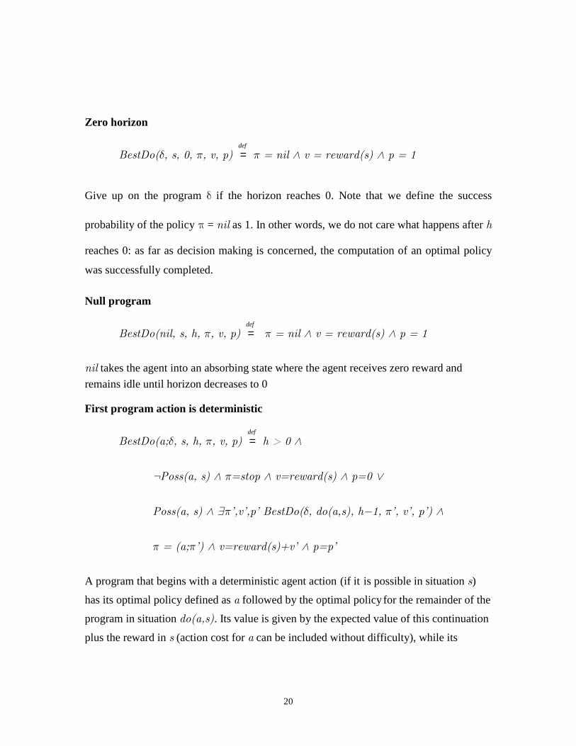
Zero horizon
BestDo(δ, s, 0, π, v, p) def
= π = nil ∧ v = reward(s) ∧ p = 1
Give up on the program δ if the horizon reaches 0. Note that we define the success
probability of the policy π = nil as 1. In other words, we do not care what happens after h
reaches 0: as far as decision making is concerned, the computation of an optimal policy
was successfully completed.
Null program
BestDo(nil, s, h, π, v, p) def
= π = nil ∧ v = reward(s) ∧ p = 1
nil takes the agent into an absorbing state where the agent receives zero reward and
remains idle until horizon decreases to 0
First program action is deterministic
BestDo(a;δ, s, h, π, v, p) def
= h > 0 ∧
¬Poss(a, s) ∧ π=stop ∧ v=reward(s) ∧ p=0 ∨
Poss(a, s) ∧ ∃π’,v’,p’ BestDo(δ, do(a,s), h−1, π’, v’, p’) ∧
π = (a;π’) ∧ v=reward(s)+v’ ∧ p=p’
A program that begins with a deterministic agent action _ (if it _ is possible in situation s )
has its optimal policy defined as a followed by the optimal policy_ _ for the remainder of the
program in situation do(a,s) . Its value is given by the expected value of this continuation
plus the reward in s (action cost for a can be included without difficulty), while its
21
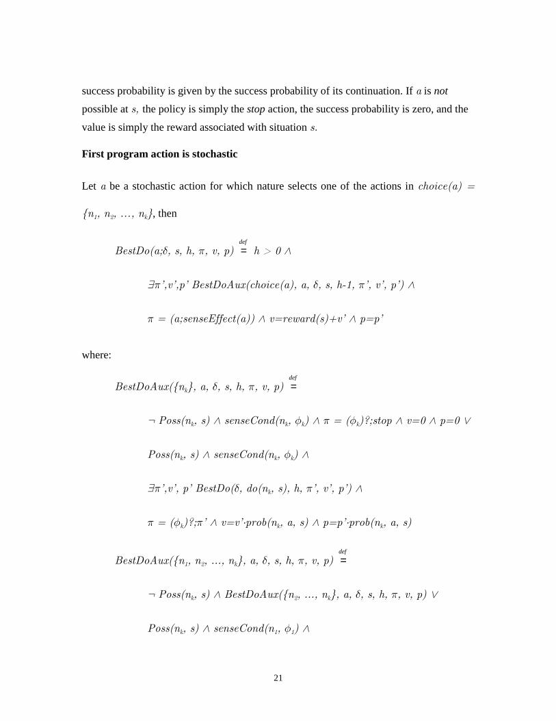
success probability is given by the success probability of its continuation. If a is not
possible at s, the policy is simply the stop action, the success probability is zero, and the
value is simply the reward associated with situation s.
First program action is stochastic
Let a be a stochastic action for which nature selects one of the actions in choice(a) =
{n1, n2, …, nk}, then
BestDo(a;δ, s, h, π, v, p) def
= h > 0 ∧
∃π’,v’,p’ BestDoAux(choice(a), a, δ, s, h-1, π’, v’, p’) ∧
π = (a;senseEffect(a)) ∧ v=reward(s)+v’ ∧ p=p’
where:
BestDoAux({nk}, a, δ, s, h, π, v, p) def
=
¬ Poss(nk, s) ∧ senseCond(nk, φk) ∧ π = (φk)?;stop ∧ v=0 ∧ p=0 ∨
Poss(nk, s) ∧ senseCond(nk, φk) ∧
∃π’,v’, p’ BestDo(δ, do(nk, s), h, π’, v’, p’) ∧
π = (φk)?;π’ ∧ v=v’⋅prob(nk, a, s) ∧ p=p’⋅prob(nk, a, s)
BestDoAux({n1, n2, ..., nk}, a, δ, s, h, π, v, p) def
=
¬ Poss(nk, s) ∧ BestDoAux({n2, ..., nk}, a, δ, s, h, π, v, p) ∨
Poss(nk, s) ∧ senseCond(n1, φ1) ∧
22
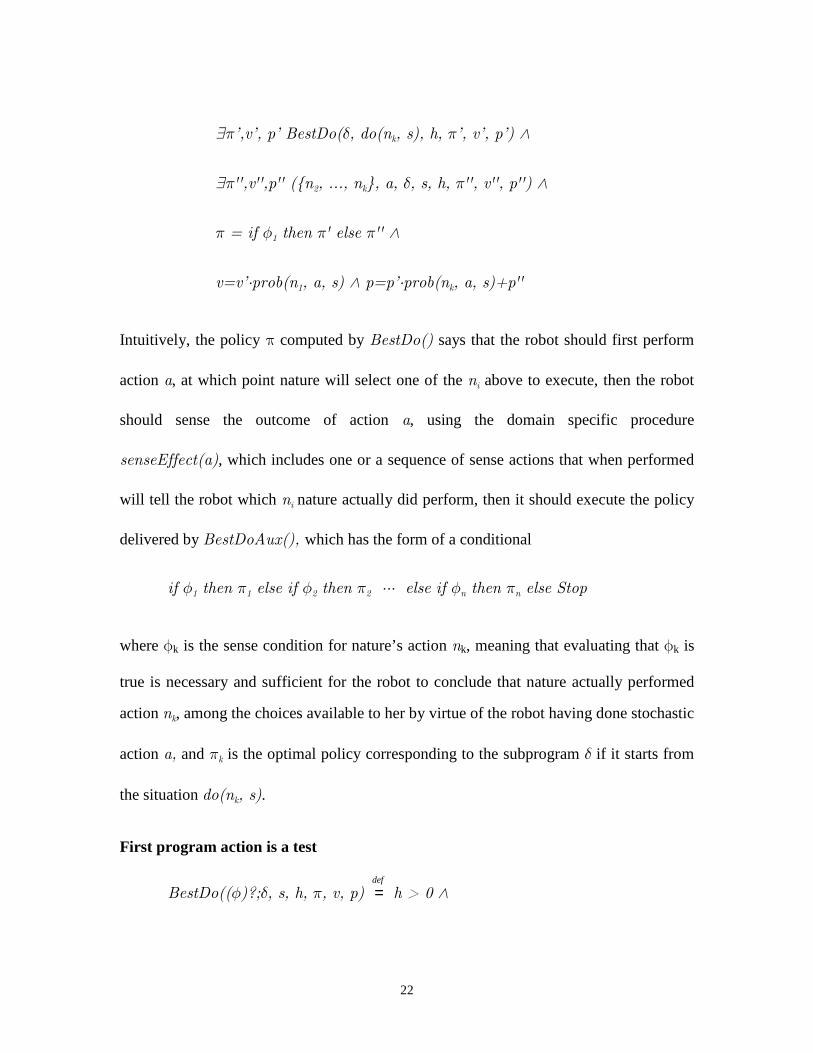
∃π’,v’, p’ BestDo(δ, do(nk, s), h, π’, v’, p’) ∧
∃π'',v'',p'' ({n2, ..., nk}, a, δ, s, h, π'', v'', p'') ∧
π = if φ1 then π' else π'' ∧
v=v’⋅prob(n1, a, s) ∧ p=p’⋅prob(nk, a, s)+p''
Intuitively, the policy π computed by BestDo() says that the robot should first perform
action a, at which point nature will select one of the ni above to execute, then the robot
should sense the outcome of action a, using the domain specific procedure
senseEffect(a), which includes one or a sequence of sense actions that when performed
will tell the robot which ni nature actually did perform, then it should execute the policy
delivered by BestDoAux(), which has the form of a conditional
if φ1 then π1 else if φ2 then π2 ⋅⋅⋅ else if φn then πn else Stop
where φk is the sense condition for nature’s action nk, meaning that evaluating that φk is
true is necessary and sufficient for the robot to conclude that nature actually performed
action nk, among the choices available to her by virtue of the robot having done stochastic
action a, and πk is the optimal policy corresponding to the subprogram δ if it starts from
the situation do(nk, s).
First program action is a test
BestDo((φ)?;δ, s, h, π, v, p) def
= h > 0 ∧
23
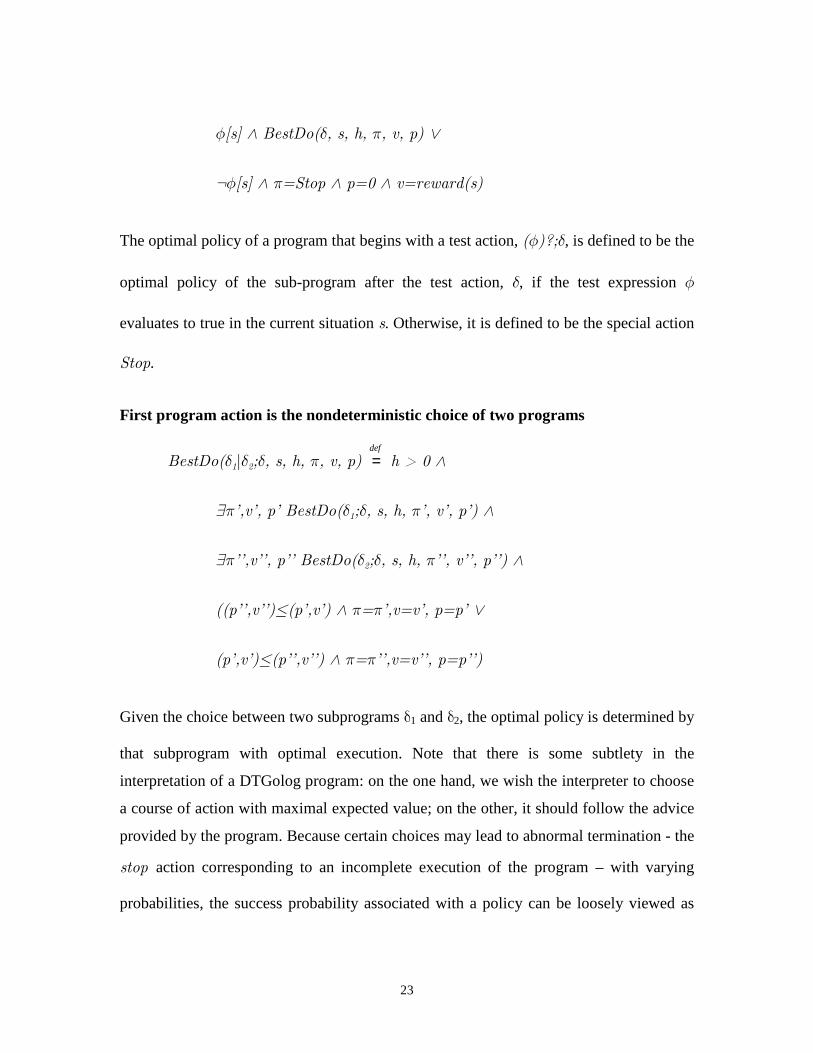
φ[s] ∧ BestDo(δ, s, h, π, v, p) ∨
¬φ[s] ∧ π=Stop ∧ p=0 ∧ v=reward(s)
The optimal policy of a program that begins with a test action, (φ)?;δ, is defined to be the
optimal policy of the sub-program after the test action, δ, if the test expression φ
evaluates to true in the current situation s. Otherwise, it is defined to be the special action
Stop.
First program action is the nondeterministic choice of two programs
BestDo(δ1|δ2;δ, s, h, π, v, p) def
= h > 0 ∧
∃π’,v’, p’ BestDo(δ1;δ, s, h, π’, v’, p’) ∧
∃π’’,v’’, p’’ BestDo(δ2;δ, s, h, π’’, v’’, p’’) ∧
((p’’,v’’)≤(p’,v’) ∧ π=π’,v=v’, p=p’ ∨
(p’,v’)≤(p’’,v’’) ∧ π=π’’,v=v’’, p=p’’)
Given the choice between two subprograms δ1 and δ2, the optimal policy is determined by
that subprogram with optimal execution. Note that there is some subtlety in the
interpretation of a DTGolog program: on the one hand, we wish the interpreter to choose
a course of action with maximal expected value; on the other, it should follow the advice
provided by the program. Because certain choices may lead to abnormal termination - the
stop action corresponding to an incomplete execution of the program – with varying
probabilities, the success probability associated with a policy can be loosely viewed as
24
the degree to which the interpreter adhered to the program. The predicate ≤ compares
pairs of the form (v, p), where p is a success probability and v is an expected value, as
follows:
(v1,p1) ≤ (v2, p2) def
= v1 ≤ v2 ∧ (p1 ≠ 0 ∧ p2 ≠ 0 ∨ p1 = 0 ∧ p2 = 0) ∨
p1 = 0 ∧ p2 ≠ 0
Nondeterministic finite choice of action arguments
If the program begins with (π(x : τ)δ) ; γ, the finite nondeterministic choice followed
sequentially by a sub-program γ, the finite set τ = {c1, c2, ... ,cn}, and the choice binds
all free occurrences of x in δ to one of these elements, then:
BestDo((π(x : τ) δ1) ; γ, s, h, π, v, p) def
= h > 0 ∧
BestDo((1
|xcδ |2
|xcδ ... |n
xcδ );γ, s, h, π, v, p).
As can be seen, the construct (π(x : τ)δ) serves as an abbreviation for the
nondeterministic program (1
|xcδ |2
|xcδ ... |n
xcδ ), where |xcδ means substitution of c for all
free occurrences of x in δ. Intuitively, this construct says that the program expression δ,
of which x is an argument, should be executed with the argument ci ∈ τ that would yield
the highest value. To do this, the DTGolog interpreter compares the values of different
arguments ci, by building and searching a decision tree that is rooted at the current
situation s, and has one branch for each ci. Please refer to section 2.3.3 for a more
detailed description of the procedural interpretation of Golog programs.
25
Nondeterministic choice of arguments
BestDo((π x)δ(x);γ, h, π, v, p) def
= h > 0 ∧
∃x BestDo(δ(x);γ, s, h, π, v, p)
This is a non-decision-theoretic version of nondeterministic choice: pick an argument and
compute an optimal policy given this argument. We need this operator because it will be
convenient to choose values of variables that satisfy certain conditions, to choose
moments of time and values returned from sensors. Note that in Golog, this operator is an
operator for choosing one of the alternatives, but in DTGolog it is used only for
programming purposes, and not for decision making.
Conditional
BestDo(if φ then δ1 else δ2 ; δ, s, h, π, v, p) def
= h > 0 ∧
φ[s] ∧ BestDo(δ1, s, h, π, v, p) ∨
¬φ[s] ∧ BestDo(δ2, s, h, π, v, p)
Let the program start with a conditional if φ then δ1 else δ2. If the test expression
evaluates to true in s, then the optimal policy must be computed using then-branch,
otherwise, the optimal policy must be computed following else-branch.
First action is a while-loop or is a procedure
The specifications of these constructs require second order logic. Please refers to [24] for
more details.
26
2.3.2.1 Incremental DTGolog Interpreter
For the purpose of introducing an online interpreter, which provides the agent with the
ability to execute actions in the real world, described in section 2.3.4 below, an
incremental version [23] of the DTGolog interpreter described above has been
introduced. This interpreter is based on the special relation IncrBestDo(δ, s, h, γ, π, v,
p), and provides the same functionality as the interpreter based on BestDo(). It
computes, as before, an optimal policy π for the Golog program δ starting from situation
s and horizon h, but in addition also computes from the program δ its sub-program γ that
remains to be executed after actually performing the first action from the policy π.
In this interpreter, two additional programming constructs are defined:
First action is the local() search control construct
IncrBestDo(local(δ1);δ, s, h, γ, π, v, p) def
= h > 0 ∧
(∃γ1, π1, v1, p1) IncrBestDo(δ1;Nil, s, h, γ1, π1, v1, p1) ∧
IncrBestDo(π1;δ, s, h, γ, π, v, p)
Instead of doing a full look-ahead to the end of the program, the interpreter begins
computing an optimal policy π1 corresponding to a smaller local sub-space of the state
space. Then, this policy can be expanded to a larger portion of the state space by
computing a policy π optimal with respect to the whole program.
First action is the limit() search control construct
27
IncrBestDo(limit(δ1);δ, s, h, γ, π, v, p) def
= h > 0 ∧
(∃γ’) IncrBestDo(δ1;Nil, s, h, γ’, π, v, p) ∧
(γ’ ≠ Nil ∧ γ = (limit(γ’); δ) ∨ γ’ = Nil ∧ γ = δ)
Without looking into δ, the incremental interpreter simply computes the policy π that is
optimal with respect to the subprogram δ1, and sets the remaining program γ to
(limit(γ’);δ), where γ’ is the sub-program that remain after the first action in π is
executed. This construct allows the programmer to express his domain-specific
procedural knowledge to save computational efforts. He can write limit(δ1);δ whenever
he knows that looking into δ has no, or very little, effects on the determination of the
initial part of the optimal policy.
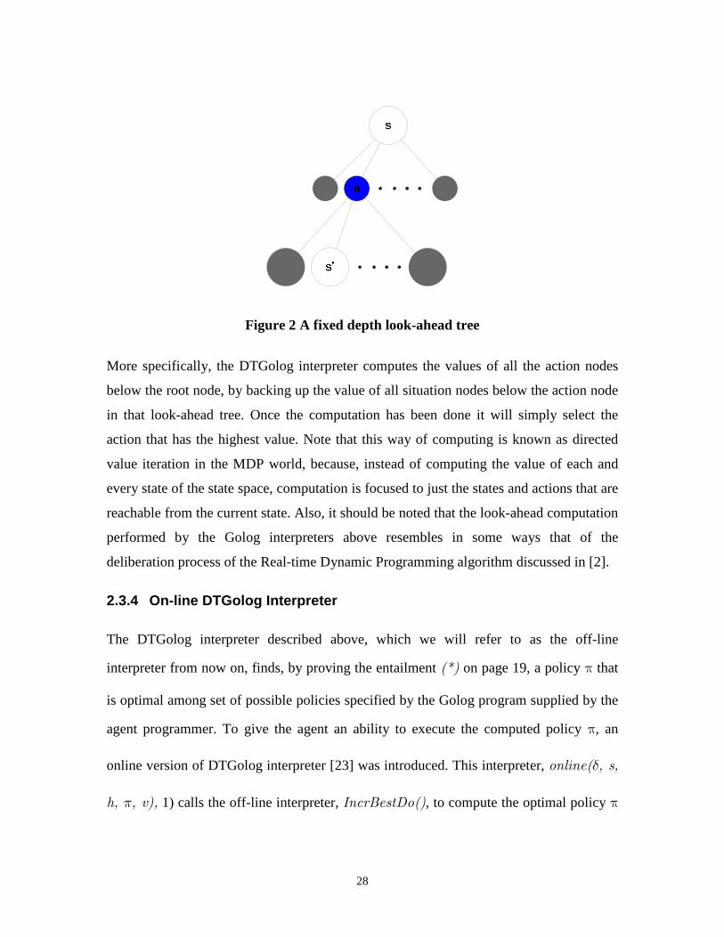
2.3.3 Procedural Interpretation
It is instructive to note that procedurally, DTGolog interpreter does decision theoretic
planning by building and searching a fixed-depth look-ahead tree that is rooted at the
current situation. Figure 2 below shows an example of such tree. The root of the tree
represents the current situation s. The dark nodes below it represent the agent actions that
are prescribed by the Golog program for s, and the large nodes below that represent the
possible next situations, and so on.
28
Figure 2 A fixed depth look-ahead tree
More specifically, the DTGolog interpreter computes the values of all the action nodes
below the root node, by backing up the value of all situation nodes below the action node
in that look-ahead tree. Once the computation has been done it will simply select the
action that has the highest value. Note that this way of computing is known as directed
value iteration in the MDP world, because, instead of computing the value of each and
every state of the state space, computation is focused to just the states and actions that are
reachable from the current state. Also, it should be noted that the look-ahead computation
performed by the Golog interpreters above resembles in some ways that of the
deliberation process of the Real-time Dynamic Programming algorithm discussed in [2].
2.3.4 On-line DTGolog Interpreter
The DTGolog interpreter described above, which we will refer to as the off-line
interpreter from now on, finds, by proving the entailment (*) on page 19, a policy π that
is optimal among set of possible policies specified by the Golog program supplied by the
agent programmer. To give the agent an ability to execute the computed policy π, an
online version of DTGolog interpreter [23] was introduced. This interpreter, online(δ, s,
h, π, v), 1) calls the off-line interpreter, IncrBestDo(), to compute the optimal policy π
29
off-line, 2) commits (i.e., executes) the first action in π, and 3) repeats the process with
the remaining parts of the program.
By giving the agent the ability to execute actions, and sense the actual next situation, the
online interpreter, in combination with the limit() search control construct, offers an
important computational advantage: Whenever it encounters (limit(δ1);δ), instead of
having to search the large decision tree corresponding to the whole program δ1;δ, the
interpreter can: (1) search the much smaller tree corresponding to the subprogram δ1 only
(which is the sub-tree rooted at the same situation as the tree corresponding to δ1;δ, but
extends only to the scope of the limit() operator), to find a partial policy π1
corresponding to δ1, (2) execute that partial policy and observe the resulting situation s’,
and then (3) search the tree rooted at s’ that corresponds to δ to find the remaining
optimal policy π. In other words, the use of limit() in the online DTGolog interpreter
helps cut down the search significantly, especially when the program δ is highly
nondeterministic.
2.4 Alternatives to DTGolog
The idea of using domain specific knowledge to temporally abstracting the action space
allowed by Golog and DTGolog, using their procedures, has also been explored in the
Options approach, described in [28]. In this approach, primitive agent actions can be
sequentially composed to create new temporally abstracted actions, called options or
macro actions. This technique allows the agent to do decision making in a smaller and
more compact (abstracted) action space. In comparison with Golog and DTGolog, the
Options approach is less expressive because, other than sequential composition, it doesn’t
30
allow complex action compositions such as conditional, loop, recursive calls and non-
deterministic choices.
The idea of allowing the agent designer (or programmer) to encode domain-specific
knowledge into a partial program that can be used to limit the set of policies the agent has
to consider has also been explored in the framework of Hierarchies of Abstract Machines
(HAMs), Programmable Hierarchic Abstract Machines (PHAMs) [16], and the ALISP
programming language [1].
In the HAMs and PHAMs framework, a partial policy is specified using a hierarchy of
abstract finite state machines, which takes as input the state of the MDP and outputs the
action to be performed by the agents, and can contain some special nondeterministic
choice states. The choice states non-deterministically select a next machine state from
predefined finite sets of available choices, and allow the agent to switch between the
policies prescribed by the partial program. In comparison to DTGolog, the HAM
approach is less convenient in terms of specifying the partial policy. In DTGolog, this
partial policy is specified using standard high-level programming constructs, while in
HAM this partial policy is specified by designing abstract finite state machines, which
can be a non-trivial task sometimes.
In the ALISP framework, the standard Lisp language is augmented with some new
nondeterministic programming constructs to create a new language that allows the agent
designer to write partial programs, which, like Golog programs and HAMs, limit the set
of policies that the agent needs to consider. In comparison to DTGolog, the ALISP
framework has two major differences. The first difference is that in ALISP, the agent
designer is expected to manually abstract the state space. That is, he has to manually
decide how states can be grouped together into groups (or abstract states) without
changing the original MDP. Golog, on the other hand, is based on situations and fluents
instead of states, and the need for state abstraction virtually does not exists. The second
difference is that domain specific characteristics such as action’s preconditions have to be
directly encoded into the partial programs, which are task-dependent by nature. In Golog,
31
environment characteristics are represented in a knowledge base that is independent of
any control procedure, and partial programs need to encode only the procedural
knowledge associated with the tasks. Finally, ALISP is a convenient tool for
Reinforcement Learning (it is based on Tom Dietterich's approach to hierarchical
reinforcement learning[9]), and cannot take advantage of an MDP model if it is provided
explicitly. However, DTGolog cannot function if a fully observable MDP is not given in
advance, but ALISP can learn from interaction with the environment. Consequently, it
would be interesting to consider a framework that takes advantages of both ALISP and
DTGolog.
32
3 A DTGolog-based
Resource Allocator for
the London Ambulance
Service
3.1 Introduction and Motivation
Although there has been a significant amount of work done in AI related to planning
under uncertainty, especially for problems in which a certain high level goal must be
satisfied with some given probability, there are still many practical domains in which the
task of designing a decision making agent that must guarantee goal satisfaction with a
sufficiently high probability is extremely difficult, due to the large number of the state
features and actions with uncertain effects. One way to ease the computational burden of
designing such an agent is to carefully refine the given high level goal into subgoals,
along with the associated subtasks that would solve these subgoals, and finally find the
primitive actions that must be executed to solve these subtasks. The reason is that this
gradual process will help the agent designer in identifying where the search between
alternatives must concentrate. That is, by going through this process, the designer will be
able to identify useful sequences, loops, conditional or recursive structures of actions that
together provide important constraints on the set of policies that need to be considered.
Once the focus point(s) of the search has been identified, and expressed as a
33
nondeterministic choice between alternatives, the original decision making problem
reduces to the task of evaluating different designs of an agent.
In this chapter, we demonstrate the applicability of the DTGolog framework to real large-
scale problems by applying it to a well-known, real world case study: The London
Ambulance Service’s Computer Aided Dispatch system (LAS-CAD) [7;13]. This case
study comes from an investigation into a failed software development project and, while
largely unknown to the AI community, has received a significant attention in software
engineering literature. It is an excellent example of a problem with probabilistic goals,
and we suggest this case study as a grand challenge for research on planning under
uncertainty.
The main contributions of this chapter are the following. We developed an extensive
logical formalization of a non-trivial domain, and demonstrated that DTGolog is well
suited to the task of evaluation of alternative designs of a decision making agent.
3.2 The London Ambulance Service (LAS)
As described in [7], the main function of the LAS is to provide emergency respond to
“999” emergency calls for the city of London. Its facilities include a Central Ambulance
Control (CAC) office, where all 999 calls are received, and several ambulance stations,
located in three (administratively divided) LAS regions: North West (NW), North East
(NE) and South (S). Generally speaking, the operation of LAS can be summarized as
follows. When an 999 emergency phone call requesting an ambulance service arrives at
the CAC, it will be answered by a Call Taker (CT). The CT will write down all necessary
details about the request on a paper form and pass it on to the Incident Reviewer (IR),
whose job is to review all the forms passed to him by all the CTs for any duplicated
request. After reviewing a form, depending on the location of the request, the IR will
forward it to one of the three Resource Allocators (RA), whose job is to decide which of
the available ambulances in his LAS region should be sent to the requested locations.
Once the RA has made his decision, he will notify the Dispatcher (DSP), who will then
34
contact the appropriate ambulance crew and give it a mobilization instruction. Once
mobilized, the ambulance will travel as quickly as possible to the incident. Upon arrival,
the ambulance’s crew would notify the DSP (e.g., by pressing buttons on the mobile
terminal inside the ambulance). It then performs on-site diagnosis on the patient and
decides whether or not the patient needs to be taken to the hospital. In some cases, this is
not necessary and the ambulance will simply go back to its base, after reporting to the
DSP that it has became available for a new assignment. Otherwise, it will quickly carry
the patient to a hospital and, after handing the patient over to the hospital’s staff, the crew
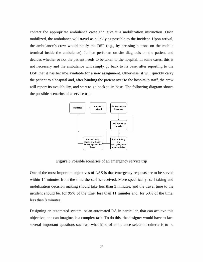
will report its availability, and start to go back to its base. The following diagram shows
the possible scenarios of a service trip.
Figure 3 Possible scenarios of an emergency service trip
One of the most important objectives of LAS is that emergency requests are to be served
within 14 minutes from the time the call is received. More specifically, call taking and
mobilization decision making should take less than 3 minutes, and the travel time to the
incident should be, for 95% of the time, less than 11 minutes and, for 50% of the time,
less than 8 minutes.
Designing an automated system, or an automated RA in particular, that can achieve this
objective, one can imagine, is a complex task. To do this, the designer would have to face
several important questions such as: what kind of ambulance selection criteria is to be
35
used; the fact that ambulances tend to travel more slowly outside their home regions, or
the fact that ambulance crews who are working on consecutive assignments without
proper resting work more slowly and less effective, should be considered; how the
communication errors that could lead to failed mobilizations, or inaccurate ambulance
location and status should be handled. For this reason, several researchers in Software
Engineering have used LAS as a case study in their works. Most notable are the
following two proposals. First, in [31], the author applied the Goal-Oriented Requirement
Language (GRL) and i* modeling framework to model and analyze the feasibility of
LAS, and concluded that the framework was capable of showing that both the totally
manual system and the fully automated system have difficulties in accomplishing LAS’s
objectives. Second, in [14], LAS is used as a case study through which new partial goal
specification and evaluation techniques, in which objective functions are specified using
probabilistic extensions of temporal logic, are illustrated.
In this work, we use LAS as a case study to show that the framework of DTGolog is not
only expressive enough to model all the above mentioned aspects but also versatile
enough to provide a quantitative evaluation of the alternative designs of a decision
making agent.
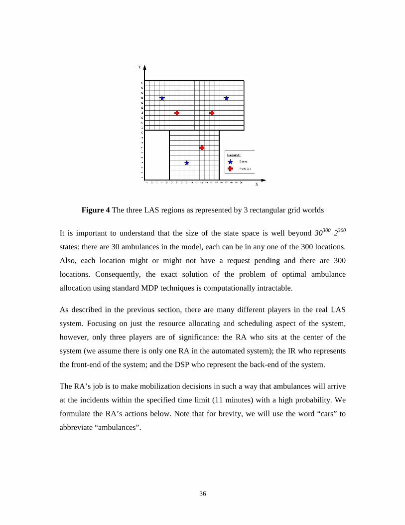
3.3 Domain Representation
We model the three LAS regions using three rectangular 10×10 grid worlds, shown in
Figure 4 below. Each square in the grid worlds represents a city block, and is denoted by
a term loc(x, y), where x and y are the block’s coordinates. All locations in the city will be
referred to by the corresponding square in which they reside, and the distance between
any two locations is defined as the Manhattan distance between the two:
d(loc(x1,y1), loc(x2,y2)) = |x2 - x1| + |y2 - y1|.
We assume that each region has one base station, one hospital, and 10 ambulances.
36
Figure 4 The three LAS regions as represented by 3 rectangular grid worlds
It is important to understand that the size of the state space is well beyond 30300⋅2300
states: there are 30 ambulances in the model, each can be in any one of the 300 locations.
Also, each location might or might not have a request pending and there are 300
locations. Consequently, the exact solution of the problem of optimal ambulance
allocation using standard MDP techniques is computationally intractable.
As described in the previous section, there are many different players in the real LAS
system. Focusing on just the resource allocating and scheduling aspect of the system,
however, only three players are of significance: the RA who sits at the center of the
system (we assume there is only one RA in the automated system); the IR who represents
the front-end of the system; and the DSP who represent the back-end of the system.
The RA’s job is to make mobilization decisions in such a way that ambulances will arrive
at the incidents within the specified time limit (11 minutes) with a high probability. We
formulate the RA’s actions below. Note that for brevity, we will use the word “cars” to
abbreviate “ambulances”.
37
• mobilize(c, l, t): Send the ambulance c to location l at time t. This is a
stochastic action with two possible outcomes: mobilizeS(c, l, t) and
mobilizeF(c, l, t). The first outcome corresponds to a successful
mobilization, and the second outcome mobilizeF corresponds to failed
mobilization (e.g., due to communication problems).
• askPosition(c, l, t): A sensing agent action that, if performed at time t, will
tell the RA the location l of car c. Because communication with the
ambulance can fail, this action can return the constant Unclear instead of a
genuine location term.
• askStatus(car, status, t): Another agent sensing action that determines
whether car is Busy, Ready, or Unknown (which means that askStatus has
failed due to communication errors).
• wait(t) A no-cost deterministic agent action that can be performed
whenever the RA has nothing to do. Doing this action will put the RA to
“sleep” until the next occurence of an exogenous event.
The IR’s job is to review emergency requests and pass them to the RA. We formulate the
IR’s actions below:
• request(l, t): Forward a reviewed emergency request to the RA. This
exogenous action means an emergency request has been made from
location l at time t.
The DSP’s job is to handle all communications between the RA and the ambulance
crews. We formulate the DSP’s actions below:
38
• reportArrival(car, l, t): Foward the arrival report of ambulance car to the
RA. This action will tell the RA that car has arrived at location l at time t.
• reportReady(car, l, t): Forward the ready report of ambulance car to the
RA. This action will tell the RA that car has become ready at location l at
time t.
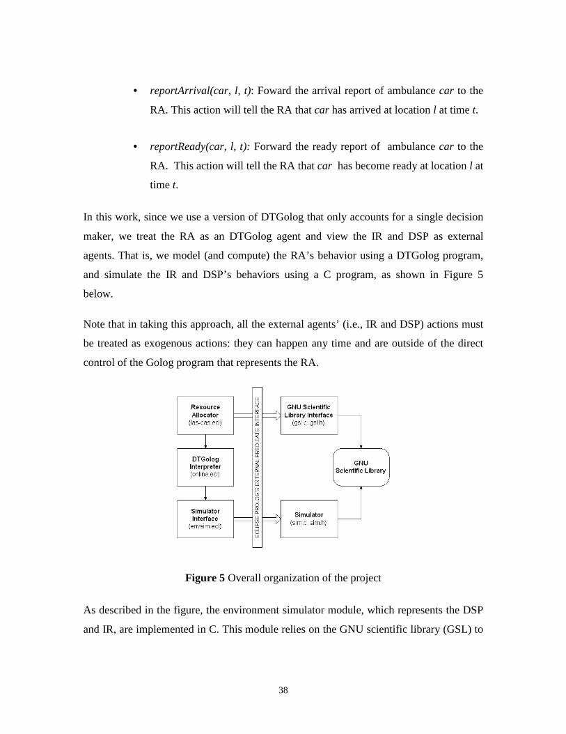
In this work, since we use a version of DTGolog that only accounts for a single decision
maker, we treat the RA as an DTGolog agent and view the IR and DSP as external
agents. That is, we model (and compute) the RA’s behavior using a DTGolog program,
and simulate the IR and DSP’s behaviors using a C program, as shown in Figure 5
below.
Note that in taking this approach, all the external agents’ (i.e., IR and DSP) actions must
be treated as exogenous actions: they can happen any time and are outside of the direct
control of the Golog program that represents the RA.
Figure 5 Overall organization of the project
As described in the figure, the environment simulator module, which represents the DSP
and IR, are implemented in C. This module relies on the GNU scientific library (GSL) to
39
generate Gaussian and Poisson random numbers, and interacts with the Golog program
(representing the RA) and the DTGolog interpreter through the simulator interface
module. The Golog program also calls on the GSL, through the GSL interface, for the
calculation of the cumulative distribution function required for the reward function
described below.
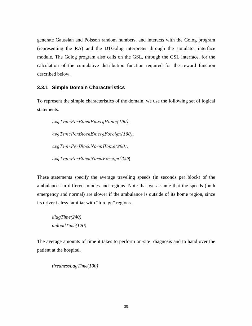
3.3.1 Simple Domain Characteristics
To represent the simple characteristics of the domain, we use the following set of logical
statements:
avgTimePerBlockEmergHome(100),
avgTimePerBlockEmergForeign(150),
avgTimePerBlockNormHome(200),
avgTimePerBlockNormForeign(250)
These statements specify the average traveling speeds (in seconds per block) of the
ambulances in different modes and regions. Note that we assume that the speeds (both
emergency and normal) are slower if the ambulance is outside of its home region, since
its driver is less familiar with “foreign” regions.
diagTime(240)
unloadTime(120)
The average amounts of time it takes to perform on-site diagnosis and to hand over the
patient at the hospital.
tirednessLagTime(100)
40
Ambulance crews that are working on consecutive assignments without having any rest
in between are tired and less efficient. If this is the case, diagnosis time, unloading time,
as well as traveling times will be longer. This statement specify the amount of extra time
it will take if the crew is tired.
requestRate(150)
commFailRate(0.15)
hospitalizeRate(0.8)
These statements specify the rate at which emergency requests arrive (in
seconds/request), the percentage at which a patient need to be taken to a hospital, and the
rate at which communication between the DSP and an ambulance traveling on the road
would fail.
validPeriod(60)
If a car is on the move, its location changes and, therefore, becomes unknown. However,
we assume that within certain grace period specified by this statement, its location has
not changed significantly and, therefore, its location is considered known.
3.3.2 More Complex Domain Characteristics
More complex domain’s characteristics are captured by the following set of axioms.
3.3.2.1 Precondition Axioms
The following axioms state that it is always possible for the RA to either wait,
askPosition or askStatus, and any value can be returned by sensing actions (i.e. sensing
results are not constrained by these axioms). Also, it is possible for a car to be mobilized
if it is ready and its location is known.
Poss(wait(t), s)
41
Poss(askPosition(car, l, t), s)
Poss(askStatus(car, status, t), s)
Poss(mobilizeS(car, loc, t), s) ≡ ready(car, s) ∧ carLocKnown(car, t, s)
Poss(mobilizeF(car, loc, t), s) ≡ ready(car, s) ∧ carLocKnown(car, t, s)
3.3.2.2 Successor state axioms & Initial Situation
A car is ready if it reported ready by itself, or if it responded Ready when the RA asked
for its status, or the car was ready in the previous situation s and the last action was
neither a successful mobilization nor a sensing action that indicates the car is busy or its
status is unknown.
ready(car, S0)
ready(car, do(a, s)) ≡ ∃l,t (a = reportReady(car, l, t)) ∨
∃t (a = askStatus(car, Ready, t)) ∨
¬∃l,t (a = mobilizeS(car, l, t)) ∧
¬∃t (a = askStatus(car, Busy, t)) ∧
¬∃t (a=askStatus(car, Unknown, t)) ∧ ready(car, s)
Communication between ambulance crews and the DSP (and hence the RA) can fail. We
model this by allowing askPosition and askStatus to return the constant Unclear and
Unknown instead of a genuine location and status3. More specifically, communication
with a given car is said to be lost if: the RA tried to ask for its location or status and the
3 By doing this, we have introduced additional states, which allow us to represent the lack of information in a fully observable MDP.
42
reply was Unclear or Unknown, or the previous mobilization failed, or communication
has been lost in the previous situation s and the car has not reported itself to the RA since
then.
commLost(car, do(a, s)) ≡ ∃t (a = askPosition(car, Unclear, t)) ∨
∃t (a = askStatus(car, Unknown, t)) ∨
∃l,t (a = mobilizeF(car, l, t)) ∨
¬∃l,t (a = reportReady(car, l, t)) ∧
¬∃l,t (a=reportArrival(car, l, t)) ∧ commLost(car, s)
When a car is stationary (e.g., parking at the home base), its location is known. When the
car is on the move, its location changes, and therefore becomes unknown. However,
recall that we assume that within the period specified by validPeriod(p), the car's location
can be considered unchanged (since it did not move very far from its last known location)
and therefore its location is known. In addition, if the car location is known in s at time
time, and it was not mobilized successfully more than p seconds ago, then its location
remains known:
carLocKnown(c, time, S0) ≡ isACar(c) ∧ start(S0, t) ∧ time >= t.
carLocKnown(c, time, do(a, s)) ≡
∃l,t((a=reportReady(c, l, t) ∨ a=askposition(c, l, t)) ∧
isBaseLoc(l) ∧ time≥ t) ∨
∃l,t,p ((a=reportReady(c, l, t) ∨ a=askposition(c, l, t)) ∧
43
validPeriod(p) ∧ time≤ t+p ∧ time≥ t) ∨
¬∃l,t,p (a = mobilizeS(c, l, t) ∧ validPeriod(p) ∧ time ≥ t + p) ∧
carLocKnown(c, time, s)
Similar to the previous axiom, the location of a car is assumed to remain the same as its
last known location within the period of p seconds.
carLocation(c, l, time, S0) ≡
isACar(c) ∧ start(S0, t) ∧ time≥ t ∧ ∃ b(homeBase(c, b) ∧ locOf(b, l))
carLocation(c, l, time, do(a, s)) ≡
∃t ((a=reportReady(c, l, t) ∨ a=askPosition(c, l, t)) ∧
isBaseLoc(l) ∧ time≥ t) ∨
∃t,p ((a=reportReady(c, l, t) ∨ a=askPosition(c, l, t)) ∧
validPeriod(p) ∧ time≤ t+p ∧ time≥ t) ∨
∃t,p,loc(a=mobilizeS(c, loc, t) ∧ validPeriod(p) ∧ time ≥ t + p ∧
l = Unknown) ∨
¬∃loc,t,p (a=mobilizeS(c, loc, t) ∧ validPeriod(p) ∧ time ≥ t + p)∧
carLocation(c, l, time, s)
44
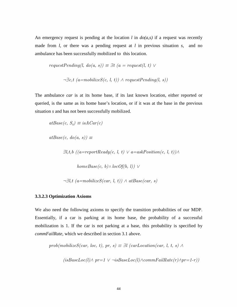
An emergency request is pending at the location l in do(a,s) if a request was recently
made from l, or there was a pending request at l in previous situation s, and no
ambulance has been successfully mobilized to this location.
requestPending(l, do(a, s)) ≡ ∃t (a = request(l, t) ∨
¬∃c,t (a=mobilizeS(c, l, t)) ∧ requestPending(l, s))
The ambulance car is at its home base, if its last known location, either reported or
queried, is the same as its home base’s location, or if it was at the base in the previous
situation s and has not been successfully mobilized.
atBase(c, S0) ≡ isACar(c)
atBase(c, do(a, s)) ≡
∃l,t,b ((a=reportReady(c, l, t) ∨ a=askPosition(c, l, t))∧
homeBase(c, b)∧ locOf(b, l)) ∨
¬∃l,t (a=mobilizeS(car, l, t)) ∧ atBase(car, s)
3.3.2.3 Optimization Axioms
We also need the following axioms to specify the transition probabilities of our MDP.
Essentially, if a car is parking at its home base, the probability of a successful
mobilization is 1. If the car is not parking at a base, this probability is specified by
commFailRate, which we described in section 3.1 above.
prob(mobilizeS(car, loc, t), pr, s) ≡ ∃l (carLocation(car, l, t, s) ∧
(isBaseLoc(l)∧ pr=1 ∨ ¬isBaseLoc(l)∧commFailRate(r)∧pr=1-r))
45
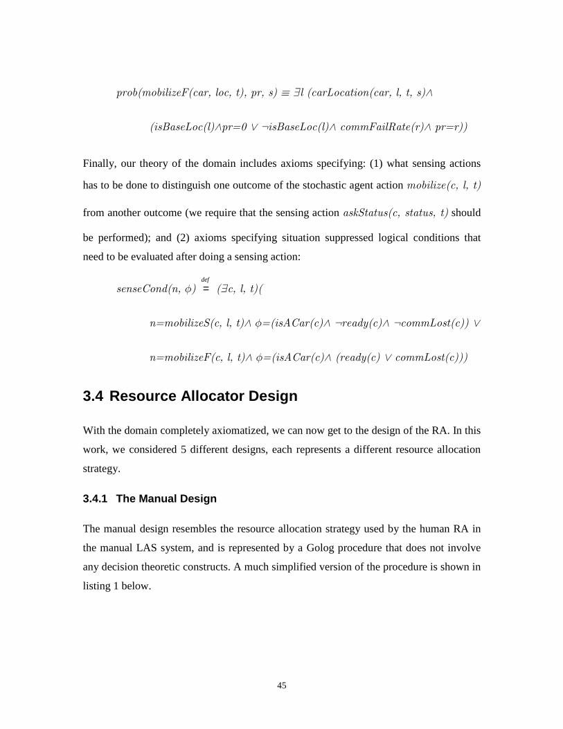
prob(mobilizeF(car, loc, t), pr, s) ≡ ∃l (carLocation(car, l, t, s)∧
(isBaseLoc(l)∧pr=0 ∨ ¬isBaseLoc(l)∧ commFailRate(r)∧ pr=r))
Finally, our theory of the domain includes axioms specifying: (1) what sensing actions
has to be done to distinguish one outcome of the stochastic agent action mobilize(c, l, t)
from another outcome (we require that the sensing action askStatus(c, status, t) should
be performed); and (2) axioms specifying situation suppressed logical conditions that
need to be evaluated after doing a sensing action:
senseCond(n, φ) def
= (∃c, l, t)(
n=mobilizeS(c, l, t)∧ φ=(isACar(c)∧ ¬ready(c)∧ ¬commLost(c)) ∨
n=mobilizeF(c, l, t)∧ φ=(isACar(c)∧ (ready(c) ∨ commLost(c)))
3.4 Resource Allocator Design
With the domain completely axiomatized, we can now get to the design of the RA. In this
work, we considered 5 different designs, each represents a different resource allocation
strategy.
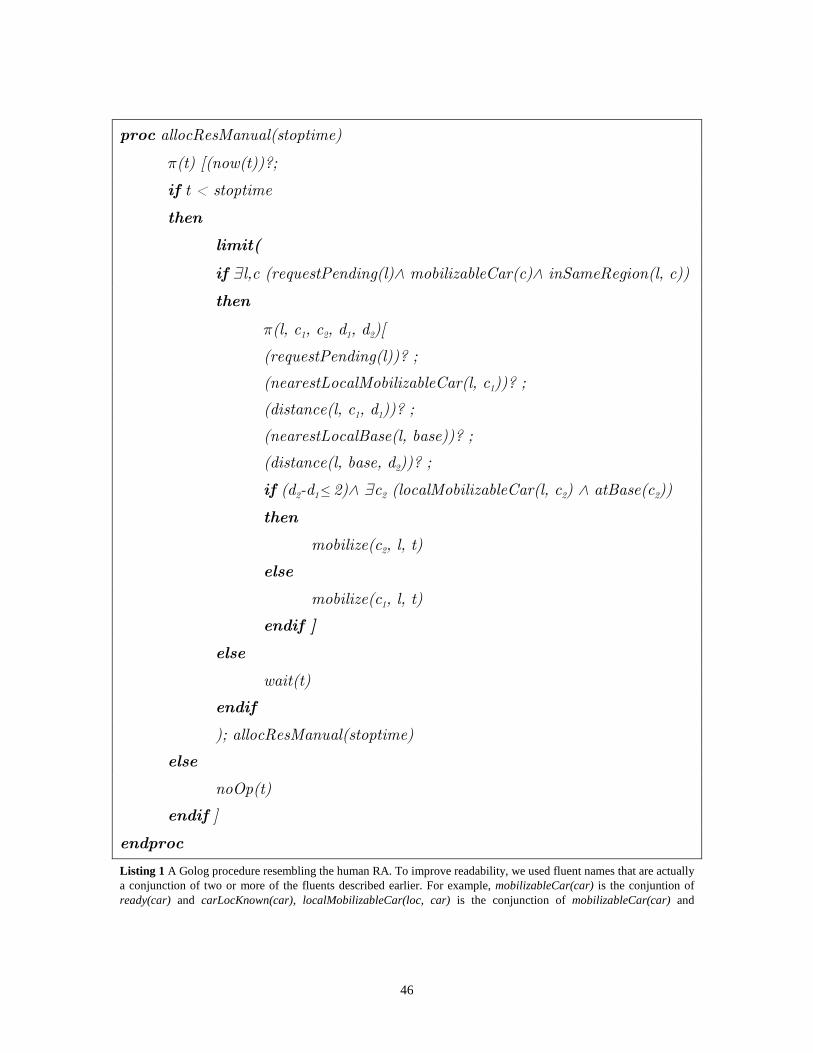
3.4.1 The Manual Design
The manual design resembles the resource allocation strategy used by the human RA in
the manual LAS system, and is represented by a Golog procedure that does not involve
any decision theoretic constructs. A much simplified version of the procedure is shown in
listing 1 below.
46
proc allocResManual(stoptime)
π(t) [(now(t))?;
if t < stoptime
then
limit(
if ∃l,c (requestPending(l)∧ mobilizableCar(c)∧ inSameRegion(l, c))
then
π(l, c1, c2, d1, d2)[
(requestPending(l))? ;
(nearestLocalMobilizableCar(l, c1))? ;
(distance(l, c1, d1))? ;
(nearestLocalBase(l, base))? ;
(distance(l, base, d2))? ;
if (d2-d1≤ 2)∧ ∃c2 (localMobilizableCar(l, c2) ∧ atBase(c2))
then
mobilize(c2, l, t)
else
mobilize(c1, l, t)
endif ]
else
wait(t)
endif
); allocResManual(stoptime)
else
noOp(t)
endif ]
endproc
Listing 1 A Golog procedure resembling the human RA. To improve readability, we used fluent names that are actually a conjunction of two or more of the fluents described earlier. For example, mobilizableCar(car) is the conjuntion of ready(car) and carLocKnown(car), localMobilizableCar(loc, car) is the conjunction of mobilizableCar(car) and

47
inSameRegion(loc, car), and nearestLocalMobilizableCar(l, c) is the conjunction of localMobilizableCar(l, car) and nearestCar(l, c)
Essentially, this Golog program, for a period of stoptime seconds, continuously checks to
see if some region is having both a pending request and a mobilizable car. If not, it will
simply perform the no cost action wait and then call itself recursively. Otherwise, the
program will locate the nearest mobilizable car c1, in the same region, and calculate its
distance d1 to the request. If this distance is not much (i.e., 2 city blocks) greater than the
distance from the request to a mobilizable car c2 that is currently parking at the base, the
program will mobilize the car at the base (c2). Otherwise, it mobilizes the nearest
mobilizable car (c1). This behavior reflects the preference that the human RA has for the
ambulances that are parking at the base over those that are current traveling on the road.
He understands that because the crews of the ambulances at the base have had proper
rest, they are more effective. So, given a choice, he will always select the ambulance
from a base unless it is much farther away from the request than is the car currently
traveling on the road.
Another important characteristic of the manual system is that, since the RAs will never
receive a request from a location outside of their region, they will never send an
ambulance across the regions’ borders. For this reason, driver’s familiarity with a region
was not considered in this Golog program, as it does not have any effect in this system.
Notice the use of the limit() search control construct in the program. This operator
prevents the off-line interpreter from searching beyond the recursive call. In the context
of this particular procedure, the use of limit() causes the agent to look ahead just enough
to make a single move. Given the complexity of the domain, and the way decisions are
made in the manual system, looking much further ahead would be both computationally
expensive and unnecessary. (Also, technically, without limit(), it would not be possible
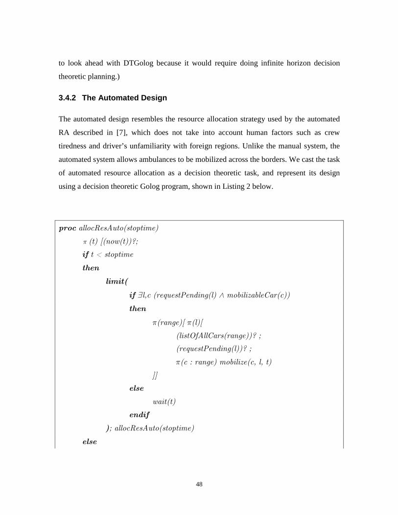
48
to look ahead with DTGolog because it would require doing infinite horizon decision
theoretic planning.)
3.4.2 The Automated Design
The automated design resembles the resource allocation strategy used by the automated
RA described in [7], which does not take into account human factors such as crew
tiredness and driver’s unfamiliarity with foreign regions. Unlike the manual system, the
automated system allows ambulances to be mobilized across the borders. We cast the task
of automated resource allocation as a decision theoretic task, and represent its design
using a decision theoretic Golog program, shown in Listing 2 below.
proc allocResAuto(stoptime)
π (t) [(now(t))?;
if t < stoptime
then
limit(
if ∃l,c (requestPending(l) ∧ mobilizableCar(c))
then
π(range)[ π(l)[
(listOfAllCars(range))? ;
(requestPending(l))? ;
π(c : range) mobilize(c, l, t)
]]
else
wait(t)
endif
); allocResAuto(stoptime)
else
49
noOp(t)
endif ]
endproc
Listing 2 A Golog procedure resembling the automated RA
The behavior of this Golog program can be described as follows. For a period of stoptime
seconds, it continuously checks to see if a request is pending and if a car, anywhere in the
city, is mobilizable. If not, it will simply perform the no cost action wait and then call
itself recursively. Otherwise, the program will select the “best” ambulance (i.e., one that
it believes to have the highest chance of getting to the incident on time) and mobilize it to
the incident. This is accomplished using the DTGolog’s construct π(c:range) that picks
the optimal car c from the finite set range of all available cars. Note that in contrast to
π(c:range), the program constructs π(range) and π(l) are not involved in decision
making. They serve simply to ground variables range and l to values specified by the
subsequent test expressions.
In order for the program to select and mobilize cars, the program needs access to a
reward function that could serve as a measure on how good or bad a mobilization
decision is. Since the automated RA doesn’t take into account crew tiredness and driver’s
region familiarity, the reward function we provided for this design depends only on the
traveling distance. That is, we define the reward r that the program can expect to receive
for mobilizing a given ambulance to a given location to be a number that is directly
proportional to the probability that the travel time is less than or equal to 11 minutes (or
660 seconds): r = c * Pr{0 ≤ T ≤ 660}, where c is a constant (e.g. 100), and T is a random
variable representing the travel time). By assuming that travel time has a Gaussian
distribution, it can be shown that T is a random variable of mean d⋅v and variance d,
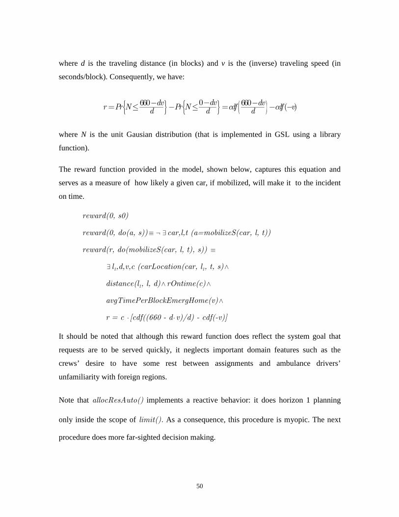
50
where d is the traveling distance (in blocks) and v is the (inverse) traveling speed (in
seconds/block). Consequently, we have:
{ } { } ( )0660 660( )
dvdv dvr Pr N Pr N cdf cdf vd d d
−− −= ≤ − ≤ = − −
where N is the unit Gausian distribution (that is implemented in GSL using a library
function).
The reward function provided in the model, shown below, captures this equation and
serves as a measure of how likely a given car, if mobilized, will make it to the incident
on time.
reward(0, s0)
reward(0, do(a, s))≡ ¬ ∃ car,l,t (a=mobilizeS(car, l, t))
reward(r, do(mobilizeS(car, l, t), s)) ≡
∃ l1,d,v,c (carLocation(car, l1, t, s)∧
distance(l1, l, d)∧ rOntime(c)∧
avgTimePerBlockEmergHome(v)∧
r = c ⋅ [cdf((660 - d ⋅v)/d) - cdf(-v)]
It should be noted that although this reward function does reflect the system goal that
requests are to be served quickly, it neglects important domain features such as the
crews’ desire to have some rest between assignments and ambulance drivers’
unfamiliarity with foreign regions.
Note that allocResAuto() implements a reactive behavior: it does horizon 1 planning
only inside the scope of limit(). As a consequence, this procedure is myopic. The next
procedure does more far-sighted decision making.
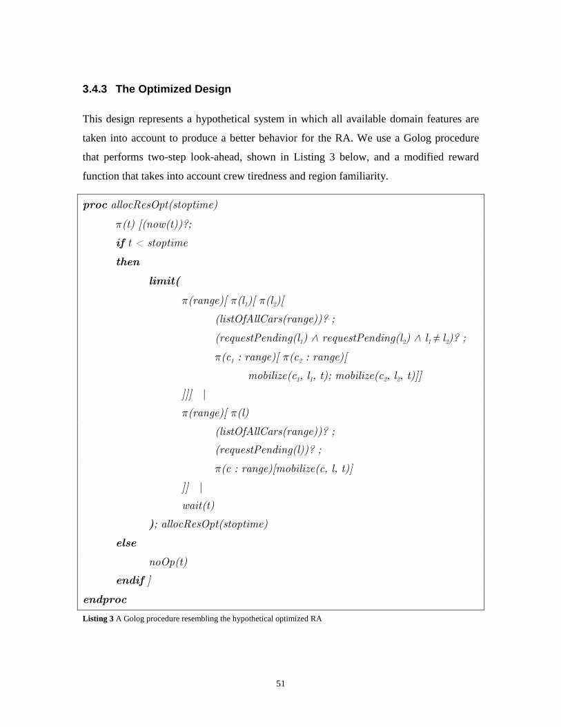
51
3.4.3 The Optimized Design
This design represents a hypothetical system in which all available domain features are
taken into account to produce a better behavior for the RA. We use a Golog procedure
that performs two-step look-ahead, shown in Listing 3 below, and a modified reward
function that takes into account crew tiredness and region familiarity.
proc allocResOpt(stoptime)
π(t) [(now(t))?;
if t < stoptime
then
limit(
π(range)[ π(l1)[ π(l2)[
(listOfAllCars(range))? ;
(requestPending(l1) ∧ requestPending(l2) ∧ l1 ≠ l2)? ;
π(c1 : range)[ π(c2 : range)[
mobilize(c1, l1, t); mobilize(c2, l2, t)]]
]]] |
π(range)[ π(l)
(listOfAllCars(range))? ;
(requestPending(l))? ;
π(c : range)[mobilize(c, l, t)]
]] |
wait(t)
); allocResOpt(stoptime)
else
noOp(t)
endif ]
endproc
Listing 3 A Golog procedure resembling the hypothetical optimized RA
52
This Golog procedure contains a nondeterministic choice between three different
branches of actions. The first branch is possible whenever there are two or more pending
requests, together with two or more mobilizable cars. The second branch is possible
whenever there is one or more pending request, together with one or more mobilizable
car. The third branch, which consists of just the zero-reward action wait(), is always
possible. When the first branch is possible, it will try to pick, by doing a horizon 2 look-
ahead, and mobilize a pair of cars that together have the highest chance of getting to both
incidents on time. Since this branch can satisfy two requests at a time, its associated value
(utility) is higher, and therefore will always be selected whenever possible (i.e., when
there are two pending requests together with two mobilizable car). If the first branch is
not possible (because there are less than two pending requests) and the second branch is
possible, it will try to pick and mobilize a car that has the highest probability of reaching
the incident on time. Since this branch can satisfy a request, it will be preferred over the
third branch whenever possible (i.e., whenever there is one pending request together with
one mobilizable car). Consequently, the behavior of this procedure can be summarized as
follows. For a period of Stoptime seconds, the procedure will continuously check to see
if there are two or more pending requests, together with two or more mobilizable cars. If
yes, it will pick and mobilize a pair of cars that together have the best chance of getting to
both incidents on time. Otherwise, it will check to see if there is one pending request,
together with a mobilizable car. If yes, it will try to pick and mobilize the car that has the
highest chance of getting to the incident on time. Otherwise, it will simply wait.
To take into account crew tiredness and region familiarity, we modify the reward
function used in the automated design above by replacing the line
“avgTimePerBlockEmergHome(v)” with the following expression:
inHomeRegion(car, l)∧ inHomeRegion(car,l1)∧
avgTimePerBlockEmergHome(v) ∨
53
¬ (inHomeRegion(car, l)∧ inHomeRegion(car,l1))∧
avgTimePerBlockEmergForeign(v)
which means that if both the source and the destination of the trip are within the home
region of the given ambulance, the traveling speed will be that of the home region (i.e.,
faster). Otherwise, the traveling speed will be that of foreign regions (i.e., slower).
We also replace “r = c * [cdf((660 - d*v)/d) - cdf(-v)]” with the conjunction:
consecTripCount(car, n, s)∧ crewTirednessLagTime(lag)
∧ r = c ⋅ [cdf((660 - n ⋅ lag - d ⋅v)/d) - cdf(-v)]
which means that if an ambulance crew has consecutively served n requests, without any
rest in between, then the reward r the program can expect to receive for mobilizing that
ambulance to a location will be equal to the probability that the ambulance will arrive at
the incident on or before (660 - n⋅ lag) seconds, which is a very small probability if lag is
sufficiently large compares to v. This, in effect, will discourage the RA from mobilizing
tired crews.
3.4.4 Other designs
As can be seen with the previous three RA designs, in the context of DTGolog, a design
is represented by a pair <P, R>, where P is a control procedure, such as allocResOpt(),
and R is a reward function. For comparison purposes, we also consider two additional
RA designs that are represented by <allocResAuto(), R2> and <allocResOpt(), R1>,
where R1 is the reward function used in the automated design, and R2 is the reward
function used in the optimized design.
54
3.5 Simulation Results
We do quantitative comparison of the 5 RA designs described above using our simulator,
which simulates the behaviors of the IR and the DSP by generating appropriate
exogenous action at specific time and in addition collects statistics about the services
trips. To simulate the behaviors of the IR, the simulator pre-calculates, at the start of each
service trip, all of its relevant time points. For example, the trip’s arrival time is pre-
calculated by adding the time it takes to travel from the base to the incident with the
starting time. Then, when these pre-calculated time points are reached, appropriate
exogenous actions will be generated accordingly. For instance, a reportArrival() will be
generated when an arrival time is reached. Randomness is introduced through the
calculation of travel times. That is, to calculate the travel times, say from l1 to l2, the
simulator uses the formula t(l1, l2) = 1( ,1)
dii
N v=∑ , where t(l1, l2) is the travel time, d is the
distance between l1 and l2,, vi is the average travel time for the current block (which
depends on whether the block is in the home or foreign region), N(vi,1) is a positive
random number drawn from the Gaussian distribution with mean vi and variance 1.
We performed simulation runs of the five designs at 5 different request rates, each rate
for 5 times, and each time for approximately 300 requests. On two AMD 1800 MHz
machines, each with 1GB of memory running Linux kernel 2.6.8, the whole process takes
approximately 12.5 hours, which means that it takes 1 minute to simulate about
(5×5×300) / (12.5×60) = 10 requests on average. Averaged simulation results, along
with their standard deviations, are plotted and shown in the tables below. Original
simulation data are also provided in Appendix D.
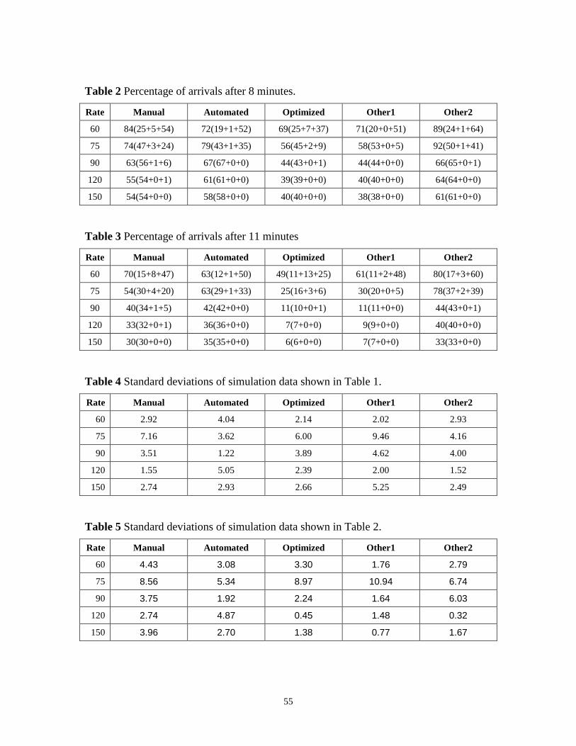
55
Table 2 Percentage of arrivals after 8 minutes.
Rate Manual Automated Optimized Other1 Other2
60 84(25+5+54) 72(19+1+52) 69(25+7+37) 71(20+0+51) 89(24+1+64)
75 74(47+3+24) 79(43+1+35) 56(45+2+9) 58(53+0+5) 92(50+1+41)
90 63(56+1+6) 67(67+0+0) 44(43+0+1) 44(44+0+0) 66(65+0+1)
120 55(54+0+1) 61(61+0+0) 39(39+0+0) 40(40+0+0) 64(64+0+0)
150 54(54+0+0) 58(58+0+0) 40(40+0+0) 38(38+0+0) 61(61+0+0)
Table 3 Percentage of arrivals after 11 minutes
Rate Manual Automated Optimized Other1 Other2
60 70(15+8+47) 63(12+1+50) 49(11+13+25) 61(11+2+48) 80(17+3+60)
75 54(30+4+20) 63(29+1+33) 25(16+3+6) 30(20+0+5) 78(37+2+39)
90 40(34+1+5) 42(42+0+0) 11(10+0+1) 11(11+0+0) 44(43+0+1)
120 33(32+0+1) 36(36+0+0) 7(7+0+0) 9(9+0+0) 40(40+0+0)
150 30(30+0+0) 35(35+0+0) 6(6+0+0) 7(7+0+0) 33(33+0+0)
Table 4 Standard deviations of simulation data shown in Table 1.
Rate Manual Automated Optimized Other1 Other2
60 2.92 4.04 2.14 2.02 2.93
75 7.16 3.62 6.00 9.46 4.16
90 3.51 1.22 3.89 4.62 4.00
120 1.55 5.05 2.39 2.00 1.52
150 2.74 2.93 2.66 5.25 2.49
Table 5 Standard deviations of simulation data shown in Table 2.
Rate Manual Automated Optimized Other1 Other2
60 4.43 3.08 3.30 1.76 2.79
75 8.56 5.34 8.97 10.94 6.74
90 3.75 1.92 2.24 1.64 6.03
120 2.74 4.87 0.45 1.48 0.32
150 3.96 2.70 1.38 0.77 1.67
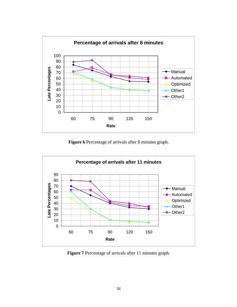
56
Percentage of arrivals after 8 minutes
0102030405060708090
100
60 75 90 120 150
Rate
Lat
e P
erce
nta
ges Manual
Automated
Optimized
Other1
Other2
Figure 6 Percentage of arrivals after 8 minutes graph.
Percentage of arrivals after 11 minutes
0102030405060708090
60 75 90 120 150
Rate
Lat
e P
erce
nta
ges
ManualAutomatedOptimizedOther1Other2
Figure 7 Percentage of arrivals after 11 minutes graph.
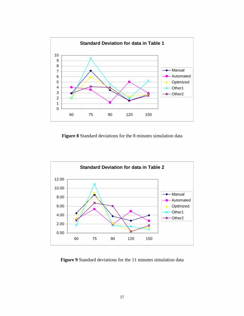
57
Standard Deviation for data in Table 1
0123456789
10
60 75 90 120 150
Manual
Automated
Optimized
Other1
Other2
Figure 8 Standard deviations for the 8 minutes simulation data
Standard Deviation for data in Table 2
0.00
2.00
4.00
6.00
8.00
10.00
12.00
60 75 90 120 150
Manual
Automated
Optimized
Other1
Other2
Figure 9 Standard deviations for the 11 minutes simulation data
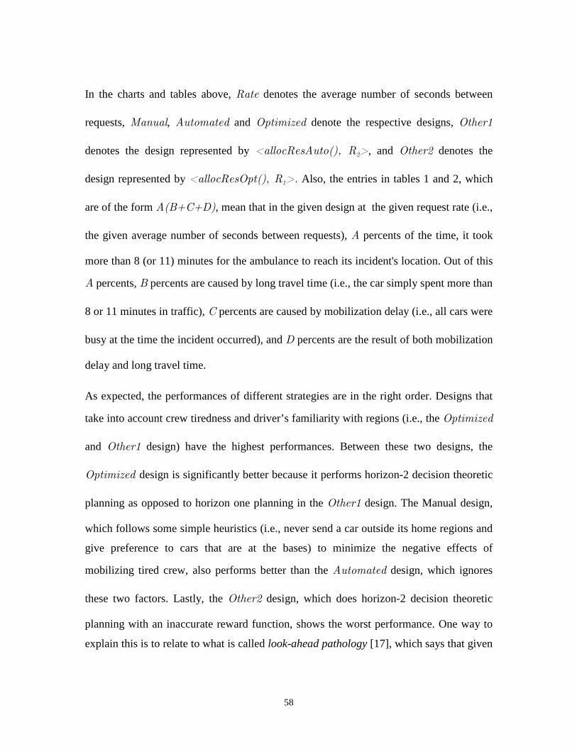
58
In the charts and tables above, Rate denotes the average number of seconds between
requests, Manual, Automated and Optimized denote the respective designs, Other1
denotes the design represented by <allocResAuto(), R2>, and Other2 denotes the
design represented by <allocResOpt(), R1>. Also, the entries in tables 1 and 2, which
are of the form A(B+C+D), mean that in the given design at the given request rate (i.e.,
the given average number of seconds between requests), A percents of the time, it took
more than 8 (or 11) minutes for the ambulance to reach its incident's location. Out of this
A percents, B percents are caused by long travel time (i.e., the car simply spent more than
8 or 11 minutes in traffic), C percents are caused by mobilization delay (i.e., all cars were
busy at the time the incident occurred), and D percents are the result of both mobilization
delay and long travel time.
As expected, the performances of different strategies are in the right order. Designs that
take into account crew tiredness and driver’s familiarity with regions (i.e., the Optimized
and Other1 design) have the highest performances. Between these two designs, the
Optimized design is significantly better because it performs horizon-2 decision theoretic
planning as opposed to horizon one planning in the Other1 design. The Manual design,
which follows some simple heuristics (i.e., never send a car outside its home regions and
give preference to cars that are at the bases) to minimize the negative effects of
mobilizing tired crew, also performs better than the Automated design, which ignores
these two factors. Lastly, the Other2 design, which does horizon-2 decision theoretic
planning with an inaccurate reward function, shows the worst performance. One way to
explain this is to relate to what is called look-ahead pathology [17], which says that given
59
the wrong value function (that represents incorrect information about the world), looking
further ahead tends to produce worse results.
Table 1 and its corresponding graph, shown in Figure 6, contain some minor irregularities
in terms of performance of a given design over different request rates. In particular, as the
request rate increases (system become less busy), the percentage of late arrivals for the
Automated and Other2 designs first increase before they actually decrease as expected.
One explanation for this is that although we collected statistics for the 8 minutes late
criteria, the optimality criteria we used in our simulation did not account for this. That is,
all the reward functions we used were designed based on whether the ambulance will get
to the incident before or after 11 minutes, not 8 minutes. Should the 8 minutes late
criteria become an important concern, we can easily modify the reward functions to
reflex this change. Another explanation is that, as table 3 and 4 show, the standard
deviations of the collected data is still high, and more simulation runs, perhaps 100 runs
for each rate, are required to obtain more accurate averages. We were not able to
complete this because simulation would take several weeks on the computer available to
us. We have completed, however, 10 addition simulation runs for each request rate, and
the collected data are available at the web address given below.
As stated in chapter 1, the primary objective of this experiment is to apply DTGolog to
the domain of the LAS to demonstrate its advantages and potentials as a quantitative tool
for evaluating and comparing different designs of decision making agents. We believe
that we have successfully achieved this objective, because we have demonstrated several
important points:
1. We were able to reason (i.e., perform decision theoretic planning) in this
extremely large scale domain. As explained in section 3.3, LAS has more than
30300⋅2300 states, and to the best of our knowledge, most (if not all) current
decision theoretic frameworks are not able to handle problems of this scale.
60
2. We were able to quickly consider as many designs as needed without having to
modify the background domain axiomatization. As explained in section 3.4.4,
each design in DTGolog is represented by a control procedure and a reward
function. As a result, new designs can be easily considered, by writing a new
control procedure and a reward function, without changing the background
domain axiomatization.
3. Unlike most of the current requirement engineering frameworks, we were able to
quantitatively, instead of qualitatively, evaluate and compare different designs.
The content of this chapter is a significantly revised and extended version of our papers
[25;26].
All relevant software (in source code) mentioned in this chapter, together with all
collected simulation data (mentioned in this Chapter), as well as additional data, can be
downloaded from:
http://www.scs.ryerson.ca/~mes/publications/LAS/
61
4 Controlling
the Sony AIBO robot
This chapter describes a software interface between the Golog family of languages and
the Tekkotsu framework (http://www.tekkotsu.org), a general application development
framework for the Sony Aibo robots developed at Carnegie-Mellon University. It also
describes in detail a small but illustrative robotics application that serves as both a test
case for the interface, and as an illustration of how hierarchical reasoning can be done in
the online version of DTGolog.
4.1 Introduction
4.1.1 The Sony AIBO Robot
Originally introduced by Sony as a household entertainment robot, the AIBO robot
(figure 1) has been quickly picked up by the robotics community around the world as a
low-cost yet feature-full robotics research platform, due to the high quality of its
hardware and software designs, together with its relatively cheap price.
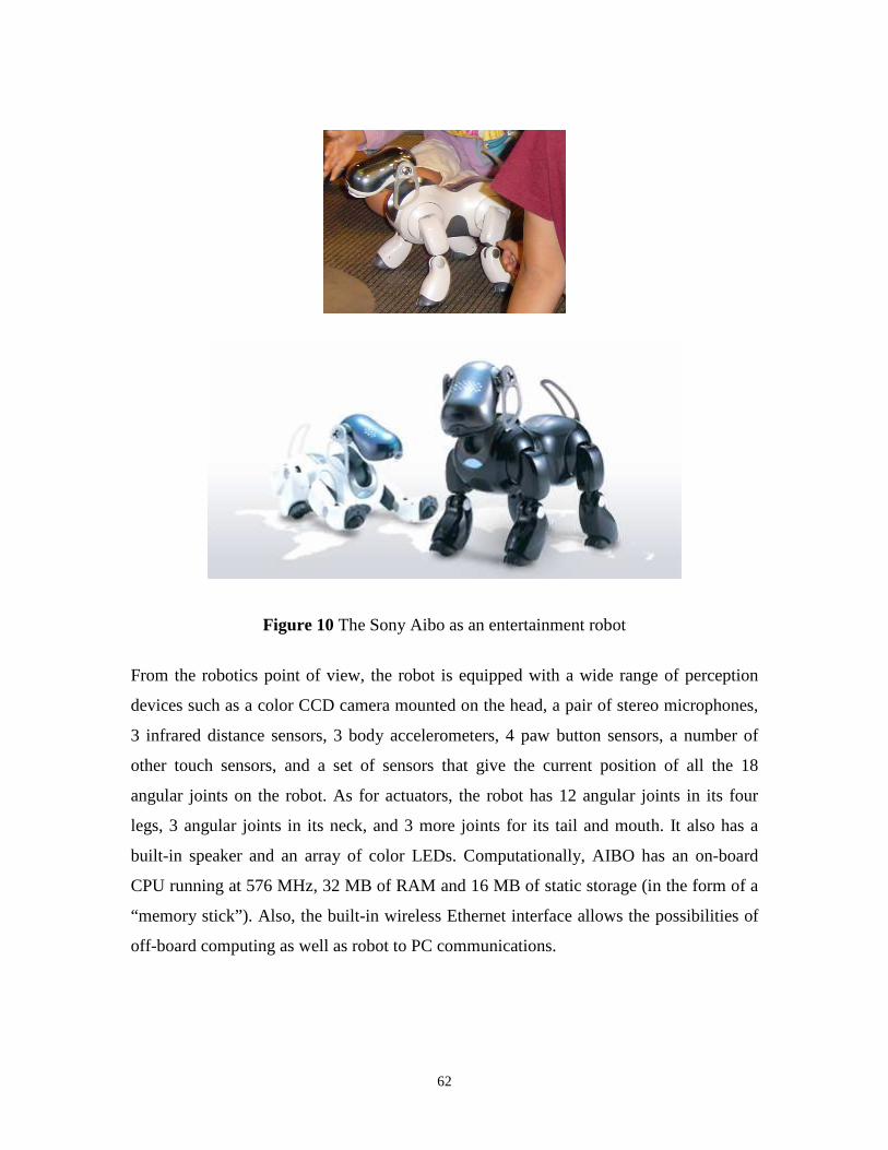
62
Figure 10 The Sony Aibo as an entertainment robot
From the robotics point of view, the robot is equipped with a wide range of perception
devices such as a color CCD camera mounted on the head, a pair of stereo microphones,
3 infrared distance sensors, 3 body accelerometers, 4 paw button sensors, a number of
other touch sensors, and a set of sensors that give the current position of all the 18
angular joints on the robot. As for actuators, the robot has 12 angular joints in its four
legs, 3 angular joints in its neck, and 3 more joints for its tail and mouth. It also has a
built-in speaker and an array of color LEDs. Computationally, AIBO has an on-board
CPU running at 576 MHz, 32 MB of RAM and 16 MB of static storage (in the form of a
“memory stick”). Also, the built-in wireless Ethernet interface allows the possibilities of
off-board computing as well as robot to PC communications.
63
4.1.2 Some well-known AIBO-based research projects
Three of the most well-known research and development projects that use AIBO as one
of the primary platforms are the Tekkotsu project, developed and maintained at CMU
with funding from Sony Corp and the two RoboSoccer projects at Carnegie-Mellon
University (CMU), headed by Manuela Veloso, and the University of Texas at Austin
(UTA), headed by Peter Stone.
In the UTA’s RoboSoccer project (http://www.cs.utexas.edu/~AustinVilla/), machine
learning techniques are applied to teach the AIBO various soccer playing skills such as
walking (i.e., running) [5;6], acquiring ball, playing keep-away [27], performing robust
localization [20] and illumination-invariant color learning [21], etc. This project has been
very successful. Among the major achievements of this project is the record-setting
walking speed attained by the AIBO, and the various prizes in yearly RoboSoccer
competitions.
The CMU RoboSoccer project (http://www.cs.cmu.edu/~robosoccer/main/) has also been
very successful. Besides winning several top prizes at RoboSoccer competitions, the
work done [29;30] in this project has served as the basis for a well-known robotics course
(http://www.cs.cmu.edu/~robosoccer/cmrobobits/) being offered at CMU. Results from
this project have also been used as important components of the Tekkotsu project, which
is described in the next paragraph.
Tekkotsu, which means “iron bone” in Japanese, is a project that aims to create an
“infrastructure for general-purpose application development on the AIBO”. It introduces
an additional abstraction layer on top of OPEN-R, Sony’s default programming interface
for the robot. Using Tekkotsu, AIBO programmers have access to an intuitive set of
primitives that are frequently encountered in robot control tasks such as perception,
manipulation, and control. This project has been a success, and research groups around
the world have adopted it into their works, mostly because it provides the AIBO robot, a
cheap yet feature-full and reliable piece of robotics hardware, with an integrated
64
framework in which not only the essential components of a typical robotics application,
such as vision and kinematics, have been integrated but also some relatively complex
predefined motions, such as walking, have been supported as library functions. The first
feature allows Tekkotsu programmer to test their ideas on a real robotics platform
without the usual overhead of manually integrating all essential robotics application
components. The second feature allows them to quickly accomplish their task by using
the supplied library actions of various levels of complexity.
The Aibo robot was also used as an experimental platform by many other researchers in
machine learning. Most related to this project is the work reported in [22], in which a
hierarchical reinforcement learning technique called Intrinsically Motivated
Reinforcement Learning (IMRL) was applied to allows Aibo to learn a two-level
hierarchy of skills: It first learns the basic skills of approaching the pink ball, capturing
and walking it, etc. and then use those basis skills to accomplish the higher level task of
locating and bringing the pink ball to its owner when requested.
4.1.3 Some potential benefits of interfacing Golog to Tekkotsu
Many robotics applications can be seen as an information channel with sensory input
signals coming in at one end and actuators commands coming out at the other end. In
between the two ends, input signals usually go through a series of transformations before
they become suitable to be used for decision making at a certain level. Then, once the
decision has been made, it will also go through some transformation process to be
eventually converted into low level actuator command signals.
The following diagram, from [8], describes the different abstraction layers through which
sensory information and command signals in an intelligent robot might go through.
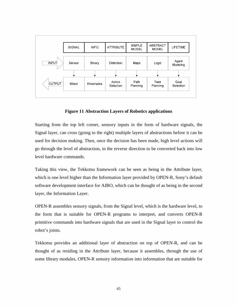
65
Figure 11 Abstraction Layers of Robotics applications
Starting from the top left corner, sensory inputs in the form of hardware signals, the
Signal layer, can cross (going to the right) multiple layers of abstractions before it can be
used for decision making. Then, once the decision has been made, high level actions will
go through the level of abstraction, in the reverse direction to be converted back into low
level hardware commands.
Taking this view, the Tekkotsu framework can be seen as being in the Attribute layer,
which is one level higher than the Information layer provided by OPEN-R, Sony’s default
software development interface for AIBO, which can be thought of as being in the second
layer, the Information Layer.
OPEN-R assembles sensory signals, from the Signal level, which is the hardware level, to
the form that is suitable for OPEN-R programs to interpret, and converts OPEN-R
primitive commands into hardware signals that are used in the Signal layer to control the
robot’s joints.
Tekkotsu provides an additional layer of abstraction on top of OPEN-R, and can be
thought of as residing in the Attribute layer, because it assembles, through the use of
some library modules, OPEN-R sensory information into information that are suitable for
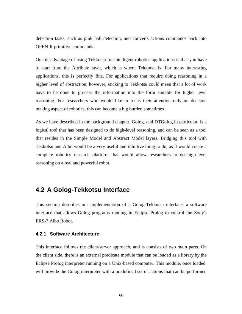
66
detection tasks, such as pink ball detection, and converts actions commands back into
OPEN-R primitive commands.
One disadvantage of using Tekkotsu for intelligent robotics applications is that you have
to start from the Attribute layer, which is where Tekkotsu is. For many interesting
applications, this is perfectly fine. For applications that require doing reasoning in a
higher level of abstraction, however, sticking to Tekkotsu could mean that a lot of work
have to be done to process the information into the form suitable for higher level
reasoning. For researchers who would like to focus their attention only on decision
making aspect of robotics, this can become a big burden sometimes.
As we have described in the background chapter, Golog, and DTGolog in particular, is a
logical tool that has been designed to do high-level reasoning, and can be seen as a tool
that resides in the Simple Model and Abstract Model layers. Bridging this tool with
Tekkotsu and Aibo would be a very useful and intuitive thing to do, as it would create a
complete robotics research platform that would allow researchers to do high-level
reasoning on a real and powerful robot.
4.2 A Golog-Tekkotsu Interface
This section describes our implementation of a Golog-Tekkotsu interface, a software
interface that allows Golog programs running in Eclipse Prolog to control the Sony's
ERS-7 Aibo Robot.
4.2.1 Software Architecture
This interface follows the client/server approach, and is consists of two main parts. On
the client side, there is an external predicate module that can be loaded as a library by the
Eclipse Prolog interpreter running on a Unix-based computer. This module, once loaded,
will provide the Golog interpreter with a predefined set of actions that can be performed
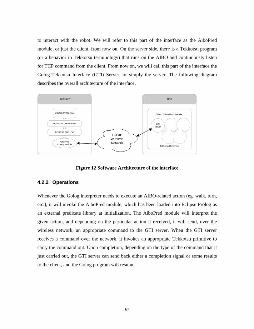
67
to interact with the robot. We will refer to this part of the interface as the AiboPred
module, or just the client, from now on. On the server side, there is a Tekkotsu program
(or a behavior in Tekkotsu terminology) that runs on the AIBO and continuously listen
for TCP command from the client. From now on, we will call this part of the interface the
Golog-Tekkotsu Interface (GTI) Server, or simply the server. The following diagram
describes the overall architecture of the interface.
UNIX HOST
ECLIPSE PROLOG
AIBO
TCP/IPWirelessNetworkAiboPred
Library Module
TEKKOTSU FRAMEWORK
GTIServer
Tekkotsu Behaviors
GOLOG INTERPRETER
GOLOG PROGRAM
Figure 12 Software Architecture of the interface
4.2.2 Operations
Whenever the Golog interpreter needs to execute an AIBO-related action (eg. walk, turn,
etc.), it will invoke the AiboPred module, which has been loaded into Eclipse Prolog as
an external predicate library at initialization. The AiboPred module will interpret the
given action, and depending on the particular action it received, it will send, over the
wireless network, an appropriate command to the GTI server. When the GTI server
receives a command over the network, it invokes an appropriate Tekkotsu primitive to
carry the command out. Upon completion, depending on the type of the command that it
just carried out, the GTI server can send back either a completion signal or some results
to the client, and the Golog program will resume.
68
4.2.3 Exported API
The list of all possible AIBO-related actions that can be executed by the Golog
interpreter, and their descriptions, is presented in Appendix A.
4.3 A test case
4.3.1 A Navigation Task
To demonstrate how this interface can be used, we consider a navigation task in which
the robot is to follow the shortest possible path to get from any room of the grid world,
see Figure 13 below, to the goal room that contains the pink ball.
Figure 13 A navigation problem
69
4.3.2 Possible approaches
4.3.2.1 Closed-loop Control Approach
This approach is probably the approach that a Tekkotsu programmer would follow. Using
this approach, the programmer would first come up with some domain-specific heuristics
and then utilize them to design an explicit program that will help AIBO to complete the
task. Given the set of tasks that have been accomplished for AIBO using this approach in
Tekkotsu, it can be said with high confidence that it is possible to solve the navigation
task above using this closed-loop control approach. It is very unlikely however, that this
approach would incorporate any model of the environment, or would involve some
probabilistic planning. For this reason, and despite the fact that it is still a research
question at this time as for whether model-based or model-free approach would be a
better choice in the longer run, we will not consider the closed-loop approach any further
here.
4.3.2.2 MDP-based Approach
Due to the probabilistic nature of the problem, that is, the uncertain outcome of many of
the possible robot actions, Markov Decision Process formalism would also sound very
appealing. One way to model the given task using this approach is to consider an MDP M
= <S, A, P, R> in which:
• A, the set of all possible robot actions, would contain the following:
o Walk(x, y, t): Walk to the location x and y, relative to the current position
of the robot, at time t.
o Turn(ang, t): Turn the whole body an angle ang at time t.
o Pan(ang, t): Pan the head an angle ang at time t.
70
o Tilt(ang, t): Tilt the head an angle ang at time t.
o Nod(ang, t): Nod the head an angle ang at time t.
o QuerySensors(pan, tilt, nod, t): Query the three head sensors at time t.
This action will tell the robot the values of its pan, tilt and nod sensors at
time t.
o QueryBall(color, visible, xcoord, ycoord, area, t): Query the robot’s
vision system regarding the ball with the given color. This action will tell
the robot whether the ball with color color is visible within the camera
image at time t or not. If yes, then what is the x and y coordinates of its
center, and the area of this ball within the image.
o SearchBall(color, found, t): Scan for the ball of the given color. This
action causes the robot to scan (i.e., move its three head joints) the space
in front of it to see if a ball with the given color can be found. If yes,
found will be set to 1, and the head will be pointing directly to the ball.
Otherwise, found will be set to 0.
o PlaySound(sound, t): Play the wave file sound at time t.
o Wait(dur, t): Simply go to sleep for dur seconds at time t.
o NoOp(t): Do nothing at time t.
• S, the set of all possible states, is represented by the 6-tuples <X, Y, θ, P, T,
N>, where X and Y represent the current absolute coordinates of the robot, θ represents
71
the angle the robot currently makes with the absolute north direction, and P, T, N
represents the current position of the robot’s pan, tilt and nod joints.
• P, the transition probabilities matrix, is a matrix that specifies, for each action a ∈
A, a current state s ∈ S, and a next state s’ ∈ S, a real probability p that represent the
probability of getting from state s to s’ by doing a.
• R, the reward function, is a function that gives, for each action a ∈ A, a current
state s ∈ S, and a next state s’ ∈ S, a reward value that represents how desirable this
transition is.
Because the state space S above is continuous (and will be a very large one if
discreetized), one would expect to encounter the following two difficulties if this
approach is to be used:
1) Computational problems with the computation of an optimal policy: Because
the state space is large (continuous), both conventional and advanced MDP techniques
would have great difficulties in computing an optimal policy for this MDP.
2) High demand on perception in physical control: Even if one assumes that a
policy can be computed for the MDP above, carrying out that policy physically requires
the robot’s ability to sense the actual current state (so that it can look up the action to be
performed from the computed policy) which, in turn, would require some advanced
sensing capabilities, such as a GPS-like device or some advanced vision facilities, which
are clearly beyond the capacity offered by the robot’s built-in perception devices.
72
4.3.2.3 DTGolog Approach
A third approach, which is the approach we took here, is to use DTGolog in such a way
that allows an intuitively clear combination of decision making and closed-loop control.
In this approach, we take advantage of the problem’s hierarchical structure to divide the
problem into two separate parts. At the top level, there is the problem of deciding the
optimal sequence of rooms the robot should visit in order to get from its current room to
the goal room as quickly as possible. (In other words, we have a path planning problem at
the top level). At the level below that, there is the problem of getting the robot to go from
one room to the next room, in the sequence computed at the top level above, as quickly as
possible. We solve the top-level problem by performing deterministic planning (or, more
precisely, probabilistic planning where all transition probabilities equal to one) in
DTGolog, and we solve the second level problem by manually writing deterministic
Golog procedures.
This way of balancing between planning and closed-loop control has been a generally
accepted practice in the robotics community. According to this practice, it is desirable
that hand-coded sub-controllers be used for sub-tasks that can be efficiently and explicitly
solved, and hence programmed, by the robot programmer, while other tasks can be left to
the robot to figure out via some deliberation processes. In the approach we took here, the
Golog procedures to get the robot from one room to another can be seen as hand-coded
sub-controllers, while the path planning problem is the deliberation process that the robot
has to go through when trying to accomplish the task as a whole.
The remaining parts of this chapter will be used to describe this approach.
4.3.3 Doing hierarchical reasoning in Online DTGolog
We propose a new way of using DTGolog that allow hierarchical reasoning as described
above to be carried out seamlessly.
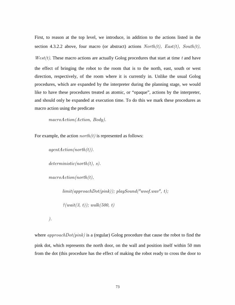
73
First, to reason at the top level, we introduce, in addition to the actions listed in the
section 4.3.2.2 above, four macro (or abstract) actions North(t), East(t), South(t),
West(t). These macro actions are actually Golog procedures that start at time t and have
the effect of bringing the robot to the room that is to the north, east, south or west
direction, respectively, of the room where it is currently in. Unlike the usual Golog
procedures, which are expanded by the interpreter during the planning stage, we would
like to have these procedures treated as atomic, or “opaque”, actions by the interpreter,
and should only be expanded at execution time. To do this we mark these procedures as
macro action using the predicate
macroAction(Action, Body).
For example, the action north(t) is represented as follows:
agentAction(north(t)).
deterministic(north(t), s).
macroAction(north(t),
limit(approachDot(pink)); playSound("woof.wav", t);
?(wait(3, t)); walk(500, t)
).
where approachDot(pink) is a (regular) Golog procedure that cause the robot to find the
pink dot, which represents the north door, on the wall and position itself within 50 mm
from the dot (this procedure has the effect of making the robot ready to cross the door to
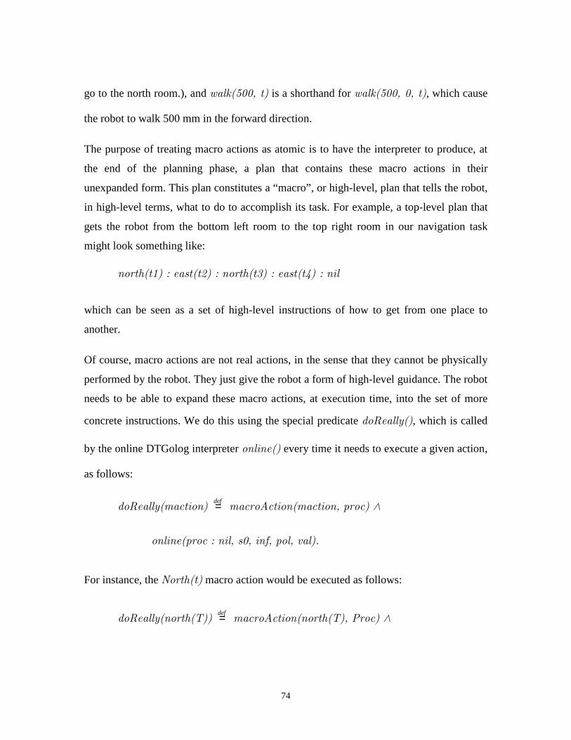
74
go to the north room.), and walk(500, t) is a shorthand for walk(500, 0, t), which cause
the robot to walk 500 mm in the forward direction.
The purpose of treating macro actions as atomic is to have the interpreter to produce, at
the end of the planning phase, a plan that contains these macro actions in their
unexpanded form. This plan constitutes a “macro”, or high-level, plan that tells the robot,
in high-level terms, what to do to accomplish its task. For example, a top-level plan that
gets the robot from the bottom left room to the top right room in our navigation task
might look something like:
north(t1) : east(t2) : north(t3) : east(t4) : nil
which can be seen as a set of high-level instructions of how to get from one place to
another.
Of course, macro actions are not real actions, in the sense that they cannot be physically
performed by the robot. They just give the robot a form of high-level guidance. The robot
needs to be able to expand these macro actions, at execution time, into the set of more
concrete instructions. We do this using the special predicate doReally(), which is called
by the online DTGolog interpreter online() every time it needs to execute a given action,
as follows:
doReally(maction) def= macroAction(maction, proc) ∧
online(proc : nil, s0, inf, pol, val).
For instance, the North(t) macro action would be executed as follows:
doReally(north(T)) def= macroAction(north(T), Proc) ∧
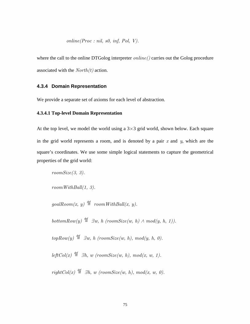
75
online(Proc : nil, s0, inf, Pol, V).
where the call to the online DTGolog interpreter online() carries out the Golog procedure
associated with the North(t) action.
4.3.4 Domain Representation
We provide a separate set of axioms for each level of abstraction.
4.3.4.1 Top-level Domain Representation
At the top level, we model the world using a 3×3 grid world, shown below. Each square
in the grid world represents a room, and is denoted by a pair x and y, which are the
square’s coordinates. We use some simple logical statements to capture the geometrical
properties of the grid world:
roomSize(3, 3).
roomWithBall(1, 3).
goalRoom(x, y) def= roomWithBall(x, y).
bottomRow(y) def= ∃w, h (roomSize(w, h) ∧ mod(y, h, 1)).
topRow(y) def= ∃w, h (roomSize(w, h), mod(y, h, 0).
leftCol(x) def= ∃h, w (roomSize(w, h), mod(x, w, 1).
rightCol(x) def= ∃h, w (roomSize(w, h), mod(x, w, 0).
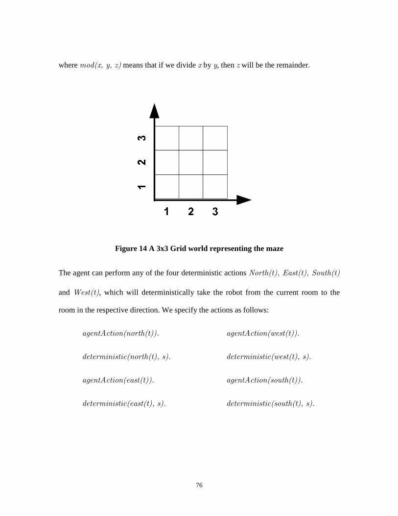
76
where mod(x, y, z) means that if we divide x by y, then z will be the remainder.
Figure 14 A 3x3 Grid world representing the maze
The agent can perform any of the four deterministic actions North(t), East(t), South(t)
and West(t), which will deterministically take the robot from the current room to the
room in the respective direction. We specify the actions as follows:
agentAction(north(t)).
deterministic(north(t), s).
agentAction(east(t)).
deterministic(east(t), s).
agentAction(west(t)).
deterministic(west(t), s).
agentAction(south(t)).
deterministic(south(t), s).
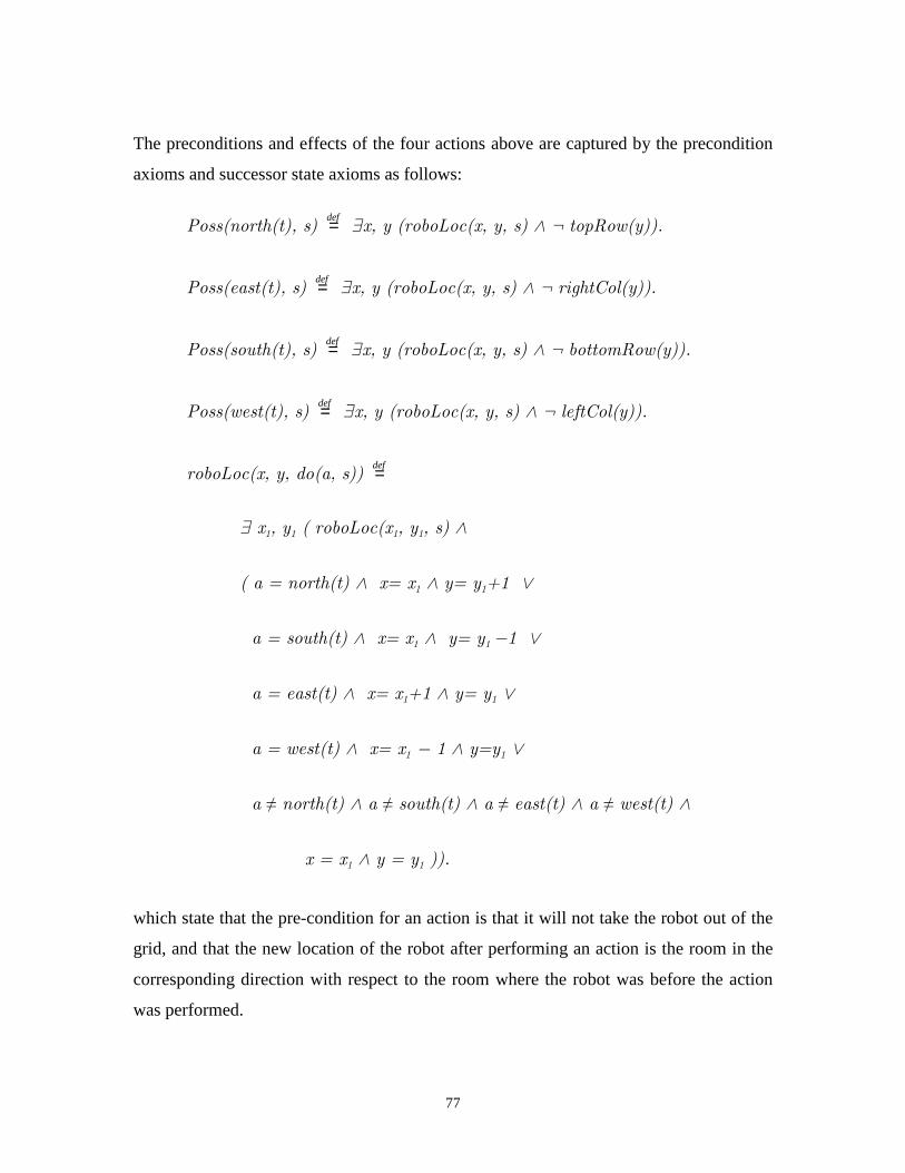
77
The preconditions and effects of the four actions above are captured by the precondition
axioms and successor state axioms as follows:
Poss(north(t), s) def= ∃x, y (roboLoc(x, y, s) ∧ ¬ topRow(y)).
Poss(east(t), s) def= ∃x, y (roboLoc(x, y, s) ∧ ¬ rightCol(y)).
Poss(south(t), s) def= ∃x, y (roboLoc(x, y, s) ∧ ¬ bottomRow(y)).
Poss(west(t), s) def= ∃x, y (roboLoc(x, y, s) ∧ ¬ leftCol(y)).
roboLoc(x, y, do(a, s)) def=
∃ x1, y1 ( roboLoc(x1, y1, s) ∧
( a = north(t) ∧ x= x1 ∧ y= y1+1 ∨
a = south(t) ∧ x= x1 ∧ y= y1 −1 ∨
a = east(t) ∧ x= x1+1 ∧ y= y1 ∨
a = west(t) ∧ x= x1 − 1 ∧ y=y1 ∨
a ≠ north(t) ∧ a ≠ south(t) ∧ a ≠ east(t) ∧ a ≠ west(t) ∧
x = x1 ∧ y = y1 )).
which state that the pre-condition for an action is that it will not take the robot out of the
grid, and that the new location of the robot after performing an action is the room in the
corresponding direction with respect to the room where the robot was before the action
was performed.
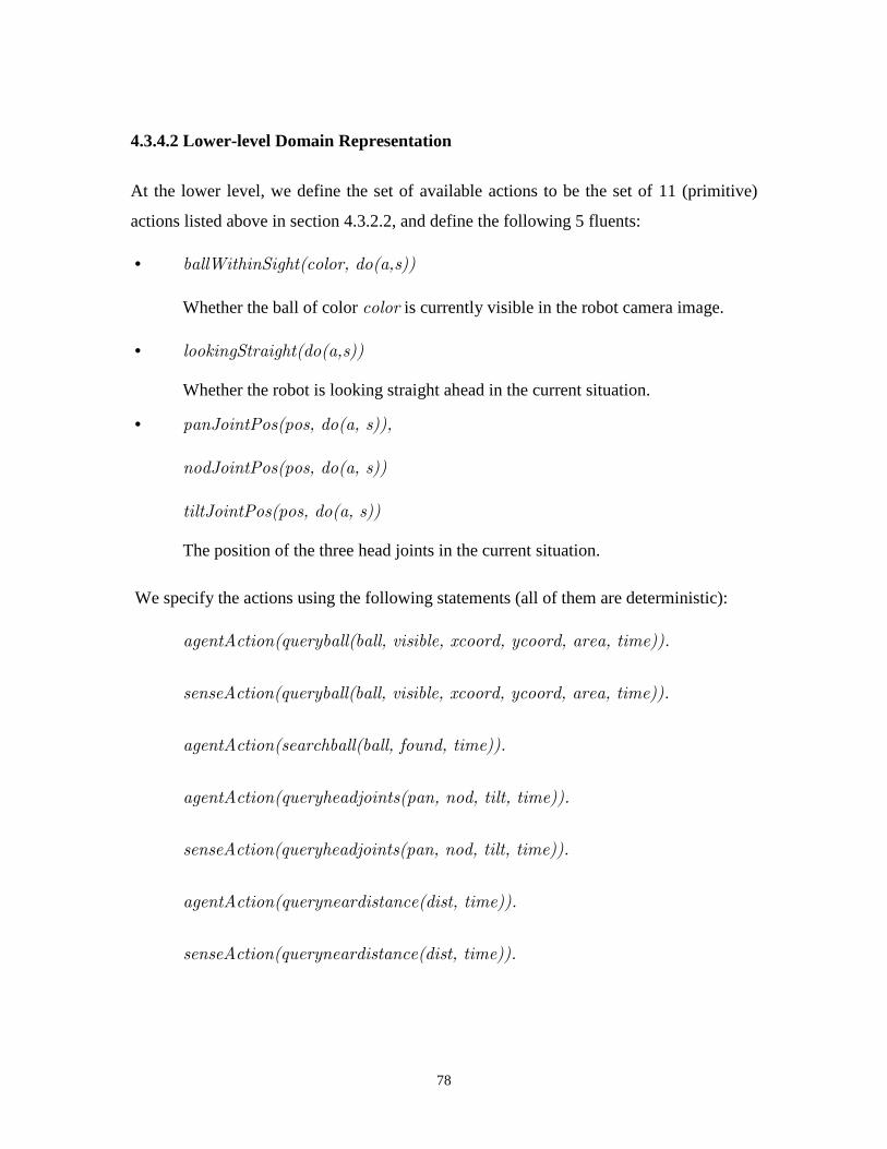
78
4.3.4.2 Lower-level Domain Representation
At the lower level, we define the set of available actions to be the set of 11 (primitive)
actions listed above in section 4.3.2.2, and define the following 5 fluents:
• ballWithinSight(color, do(a,s))
Whether the ball of color color is currently visible in the robot camera image.
• lookingStraight(do(a,s))
Whether the robot is looking straight ahead in the current situation.
• panJointPos(pos, do(a, s)),
nodJointPos(pos, do(a, s))
tiltJointPos(pos, do(a, s))
The position of the three head joints in the current situation.
We specify the actions using the following statements (all of them are deterministic):
agentAction(queryball(ball, visible, xcoord, ycoord, area, time)).
senseAction(queryball(ball, visible, xcoord, ycoord, area, time)).
agentAction(searchball(ball, found, time)).
agentAction(queryheadjoints(pan, nod, tilt, time)).
senseAction(queryheadjoints(pan, nod, tilt, time)).
agentAction(queryneardistance(dist, time)).
senseAction(queryneardistance(dist, time)).
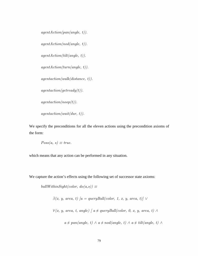
79
agentAction(pan(angle, t)).
agentAction(nod(angle, t)).
agentAction(tilt(angle, t)).
agentAction(turn(angle, t)).
agentaction(walk(distance, t)).
agentaction(getready(t)).
agentaction(noop(t)).
agentaction(wait(dur, t)).
We specify the preconditions for all the eleven actions using the precondition axioms of
the form:
Poss(a, s) ≡ true.
which means that any action can be performed in any situation.
We capture the action’s effects using the following set of successor state axioms:
ballWithinSight(color, do(a,s)) ≡
∃(x, y, area, t) [a = queryBall(color, 1, x, y, area, t)] ∨
∀(x, y, area, t, angle) [ a ≠ queryBall(color, 0, x, y, area, t) ∧
a ≠ pan(angle, t) ∧ a ≠ nod(angle, t) ∧ a ≠ tilt(angle, t) ∧
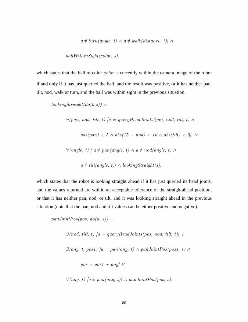
80
a ≠ turn(angle, t) ∧ a ≠ walk(distance, t)] ∧
ballWithinSight(color, s).
which states that the ball of color color is currently within the camera image of the robot
if and only if it has just queried the ball, and the result was positive, or it has neither pan,
tilt, nod, walk or turn, and the ball was within sight in the previous situation.
lookingStraight(do(a,s)) ≡
∃(pan, nod, tilt, t) [a = queryHeadJoints(pan, nod, tilt, t) ∧
abs(pan) < 5 ∧ abs(15 − nod) < 10 ∧ abs(tilt) < 5] ∨
∀(angle, t) [ a ≠ pan(angle, t) ∧ a ≠ nod(angle, t) ∧
a ≠ tilt(angle, t)] ∧ lookingStraight(s).
which states that the robot is looking straight ahead if it has just queried its head joints,
and the values returned are within an acceptable tolerance of the straigh-ahead position,
or that it has neither pan, nod, or tilt, and it was looking straight ahead in the previous
situation (note that the pan, nod and tilt values can be either positive and negative).
panJointPos(pos, do(a, s)) ≡
∃(nod, tilt, t) [a = queryHeadJoints(pos, nod, tilt, t)] ∨
∃(ang, t, pos1) [a = pan(ang, t) ∧ panJointPos(pos1, s) ∧
pos = pos1 + ang] ∨
∀(ang, t) [a ≠ pan(ang, t)] ∧ panJointPos(pos, s).
81
which states that the robot’s pan joint is currently at position pos if and only if it has just
queried that joint, and the value returned is equal to pos, or it has panned its head to the
position pos from the previous postion pos1, or, it has not panned its head, and the pan
position was pos in the previous situation.
Similar successor state axioms are provided for the nodJointPos(pos, do(a, s)) and
tiltJointPos(pos, do(a, s)) fluents.
4.3.5 Control Procedures
Similar to the domain axiom, we provide two separate sets of control procedures, one for
each level of abstraction.
4.3.5.1 Top-level control procedure
Control at the top level is very simple. The following procedure helps to plan the best
sequence of high-level moves to get from the current room to the goal room. It takes as
input the number n of moves allowed and produces an n-steps plan by non-
deterministically choosing between the four actions north(t), east(t), south(t) and
west(t).
proc(pathPlanning(n),
π(t, π(n1,
?(now(t)) :
if n < 1 then
noOp(t),
82
else
( north(t) # east(t) # south(t) # west(t) ) :
?(n1 is n − 1) : pathPlanning(n1)
endif
))
).
4.3.5.2 Lower-level control procedures
Once a high-level plan has been produced and passed to the execution unit, the macro
actions that appear in that plan will be expanded, as described in section 4.3.3, into a
lower level procedure, which will then be passed to a recursive call of the DTGolog
interpreter. The four macro actions will be expanded into the following procedures:
macroAction(north(t),
limit(approachDot(pink)) : playSound("woof.wav", t) :
?(wait(3, t)) : walk(500, t)
).
83
macroAction(east(t),
limit(approachDot(yellow)) : playSound("woof.wav", t) :
?(wait(3, t)) : walk(500, t)
).
macroAction(south(t),
limit(approachDot(blue)) : playSound("woof.wav", t) :
?(wait(3, t)) : walk(500, t)
).
macroAction(west(t),
limit(approachDot(orange)) : playSound("woof.wav", t) :
?(wait(3, t)) : walk(500, t)
).
where walk(500, t) is the shorthand for walk(500, 0, t) and approachDot(color) is a
deterministic procedure that brings the robot close (within 55 mm) to the dot of specified
color. Because each door has a unique color dot assigned to it, getting close to the door
has the effect of making the robot ready to cross through the door, and get to the room in
84
the specified direction. Once the robot is close to the desired door, and ready to go
through, it will make a barking sound (woof.wav) to request the removal of the door and
wait for 3 seconds. After 3 seconds, the door has been removed, and the robot will simply
walk straight ahead for 500 mm to enter the desired room. The limit() operators are used
to prevent DTGolog to search beyond the approachDot() procedure: Intuitively, not
until it has successfully approached the color dot, the robot should not only worry about
barking or walking head.
The definition of the approachDot(color) procedure is given below. (We write this
procedure in Golog because we want to demonstrate how Golog sub-controllers can be
used in the online version of DTGolog, and how Aibo primitive actions can be performed
using the GTI interface).
proc approachDot(color)
π(t)[ (now(t))?;
π(pval, nval, tval, vis, xcoord, ycoord, area, dist)[
limit( queryHeadJoints(pval, nval, tval, t);
queryBall(color, vis, xcoord, ycoord, area, t);
queryNearDistance(dist, t) );
if (lookingStraight ∧ ballWithinSight(color) ∧ dist < 55) then
noOp(t)
else
π(found, pval1, nval1, tval1, dist1, pval1abs, pval1less, p, n)[
limit( searchBall(color, found, t) :
queryHeadJoints(pval1, nval1, tval1, t) :
queryNearDistance(dist1, t) );
limit( ?(abs(pval1, pval1abs)) :
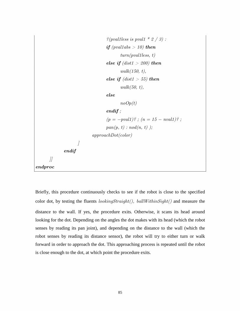
85
?(pval1less is pval1 * 2 / 3) :
if (pval1abs > 10) then
turn(pval1less, t)
else if (dist1 > 200) then
walk(150, t),
else if (dist1 > 55) then
walk(50, t),
else
noOp(t)
endif ;
(p = −pval1)? ; (n = 15 − nval1)? ;
pan(p, t) : nod(n, t) );
approachDot(color)
]
endif
]]
endproc
Briefly, this procedure continuously checks to see if the robot is close to the specified
color dot, by testing the fluents lookingStraight(), ballWithinSight() and measure the
distance to the wall. If yes, the procedure exits. Otherwise, it scans its head around
looking for the dot. Depending on the angles the dot makes with its head (which the robot
senses by reading its pan joint), and depending on the distance to the wall (which the
robot senses by reading its distance sensor), the robot will try to either turn or walk
forward in order to approach the dot. This approaching process is repeated until the robot
is close enough to the dot, at which point the procedure exits.
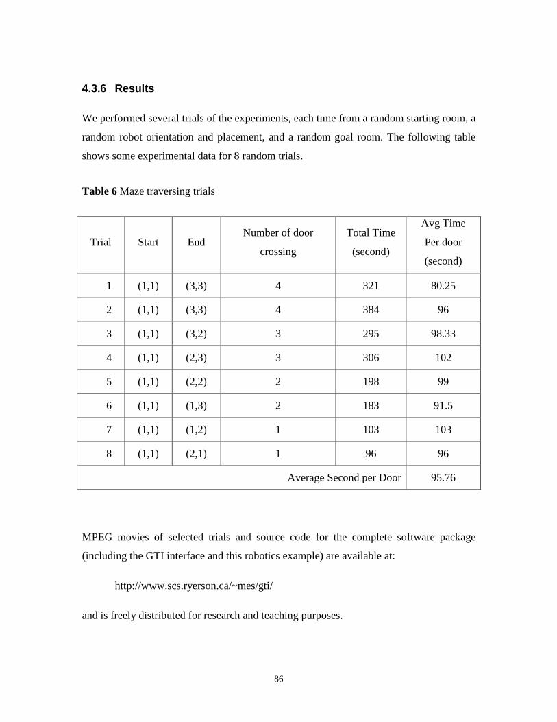
86
4.3.6 Results
We performed several trials of the experiments, each time from a random starting room, a
random robot orientation and placement, and a random goal room. The following table
shows some experimental data for 8 random trials.
Table 6 Maze traversing trials
Trial Start End Number of door
crossing
Total Time
(second)
Avg Time
Per door
(second)
1 (1,1) (3,3) 4 321 80.25
2 (1,1) (3,3) 4 384 96
3 (1,1) (3,2) 3 295 98.33
4 (1,1) (2,3) 3 306 102
5 (1,1) (2,2) 2 198 99
6 (1,1) (1,3) 2 183 91.5
7 (1,1) (1,2) 1 103 103
8 (1,1) (2,1) 1 96 96
Average Second per Door 95.76
MPEG movies of selected trials and source code for the complete software package
(including the GTI interface and this robotics example) are available at:
http://www.scs.ryerson.ca/~mes/gti/
and is freely distributed for research and teaching purposes.
87
5 Conclusion
This chapter provides a brief summary of the results reported in this thesis. It also
discusses the contributions made by this thesis and some possible future research
directions.
5.1 Summary
Probabilistic or decision theoretic planning is a very desirable tool in the fields of AI and
Robotics. Given the complete and accurate model of the world’s dynamics, decision
theoretic planning provides a decision making agent not only with the ability to figure out
the way to accomplish its goals but also with the ability to accomplish these goals in the
optimal way. Despite the fact that a lot of research efforts have been contributed to this
field, current techniques still have difficulties with real-world and large-scale
applications. DTGolog is a promising logic-based decision theoretic planning framework
that has the potential of handling real-world applications because it allows domain-
specific knowledge to be utilized as “advices” that constrain the search space into
practical size. This thesis advocates the practicality and usefulness of DTGolog by (1)
applying it to a real-world and complex domain of the London Ambulance Service, to
demonstrate its expressiveness and applicability, and by (2) bridging it to the popular and
powerful robotics platform of the Sony’s Aibo Robot, via the Tekkotsu framework, to
create a complete cognitive robotics research platform in which DTGolog can be used.
88
5.2 Contributions
The contribution of the research work reported here are as follows:
1) We have revised the DTGolog interpreter to allow it to make use of the new
linear constraints solver with a different API that is available in Eclipse Prolog, a well-
known Prolog interpreter developed at IC-PARC (a research and development company
at Imperial College, London, UK)4, version 5.7 and above, instead of the solver available
in Eclipse Prolog version 3.5.2 and below. This revision allows DTGolog to be used with
more recent versions of Eclipse Prolog and solve temporal constraints in Golog programs
more efficiently using the well-known commercial-grade linear constraint solver by
ILOG, a well-known mathematical optimization software company5.
2) We have demonstrated the expressiveness and applicability of the DTGolog
framework on large-scale problems by building and analyzing an extensive logical
formalization [25;26], plus an environment simulator and a simulator interface, for a
well-known case study, the London Ambulance Service’s Computer Aided Dispatch
System.
3) We have implemented and demonstrated a software interface that brings
DTGolog’s high-level reasoning and decision theoretic planning capabilities to the Sony
AIBO robot’s powerful, reliable yet inexpensive robotics platform to create a complete
research robotics platform that provides AI and Robotics researchers with the ability to
conveniently do high-level reasoning on a real and powerful robot. This platform can be
used as a platform for doing research in cognitive robotics, and can serve as a basis for a
future graduate course on the same topic.
4 http://eclipse.crosscoreop.com/eclipse/index.html
5 http://www.ilog.com/
89
5.3 Future Works
Two of the most important directions for future research with DTGolog are the scalability
of the DTGolog framework and the incorporation of learning into the framework.
Scalability can be improved by using sampling techniques to deal with large branching
factor (in the version of directed value iteration that provides semantics for a DTGolog
interpreter DTGolog) and by using progression to deal with growing situation terms. Our
research goal is a more advanced framework that can handle models that are large enough
to be of use in software design applications such as the current LAS-CAD system. In
2004, the real LAS-CAD system has about 30 regions, about 400 vehicles and was the
largest public ambulance system in the world.
Learning would also be a nice feature to have in DTGolog. As of current, the interpreter
can only do planning, and expects both the reward and transition probabilities functions
to be completely specified (by the reward() and prob() predicates). If learning can be
incorporated into DTGolog, DTGolog-based agents will have the ability to figure out the
optimal behavior by interacting with their environments, and will not require the
knowledge of a complete transition probabilities function.
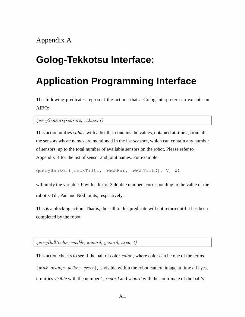
A.1
Appendix A
Golog-Tekkotsu Interface:
Application Programming Interface
The following predicates represent the actions that a Golog interpreter can execute on
AIBO:
querySensors(sensors, values, t)
This action unifies values with a list that contains the values, obtained at time t, from all
the sensors whose names are mentioned in the list sensors, which can contain any number
of sensors, up to the total number of available sensors on the robot. Please refer to
Appendix B for the list of sensor and joint names. For example:
querySensor([neckTilt1, neckPan, neckTilt2], V, 0)
will unify the variable V with a list of 3 double numbers corresponding to the value of the
robot’s Tilt, Pan and Nod joints, respectively.
This is a blocking action. That is, the call to this predicate will not return until it has been
completed by the robot.
queryBall(color, visible, xcoord, ycoord, area, t)
This action checks to see if the ball of color color , where color can be one of the terms
{pink, orange, yellow, green}, is visible within the robot camera image at time t. If yes,
it unifies visible with the number 1, xcoord and ycoord with the coordinate of the ball’s
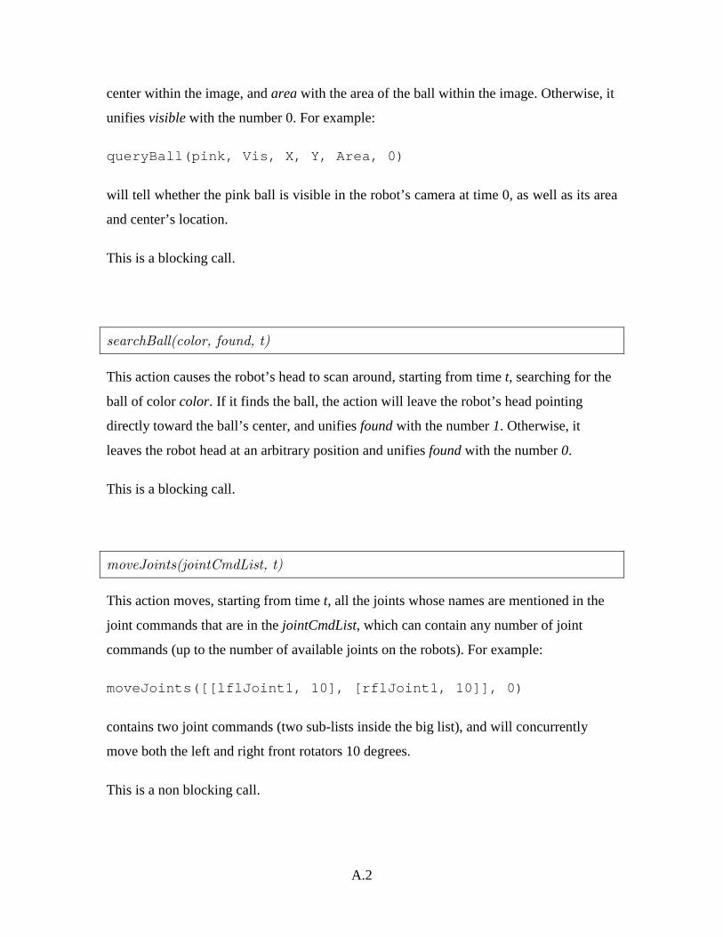
A.2
center within the image, and area with the area of the ball within the image. Otherwise, it
unifies visible with the number 0. For example:
queryBall(pink, Vis, X, Y, Area, 0)
will tell whether the pink ball is visible in the robot’s camera at time 0, as well as its area
and center’s location.
This is a blocking call.
searchBall(color, found, t)
This action causes the robot’s head to scan around, starting from time t, searching for the
ball of color color. If it finds the ball, the action will leave the robot’s head pointing
directly toward the ball’s center, and unifies found with the number 1. Otherwise, it
leaves the robot head at an arbitrary position and unifies found with the number 0.
This is a blocking call.
moveJoints(jointCmdList, t)
This action moves, starting from time t, all the joints whose names are mentioned in the
joint commands that are in the jointCmdList, which can contain any number of joint
commands (up to the number of available joints on the robots). For example:
moveJoints([[lflJoint1, 10], [rflJoint1, 10]], 0)
contains two joint commands (two sub-lists inside the big list), and will concurrently
move both the left and right front rotators 10 degrees.
This is a non blocking call.
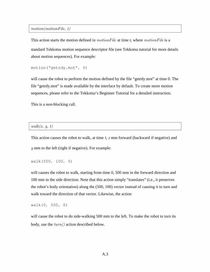
A.3
motion(motionFile, t)
This action starts the motion defined in motionFile at time t, where motionFile is a
standard Tekkotsu motion sequence descriptor file (see Tekkotsu tutorial for more details
about motion sequences). For example:
motion(“getrdy.mot”, 0)
will cause the robot to perform the motion defined by the file “getrdy.mot” at time 0. The
file “getrdy.mot” is made available by the interface by default. To create more motion
sequences, please refer to the Tekkotsu’s Beginner Tutorial for a detailed instruction.
This is a non-blocking call.
walk(x, y, t)
This action causes the robot to walk, at time t, x mm forward (backward if negative) and
y mm to the left (right if negative). For example:
walk(500, 100, 0)
will causes the robot to walk, starting from time 0, 500 mm in the forward direction and
100 mm in the side direction. Note that this action simply “translates” (i.e., it preserves
the robot’s body orientation) along the (500, 100) vector instead of causing it to turn and
walk toward the direction of that vector. Likewise, the action
walk(0, 500, 0)
will cause the robot to do side-walking 500 mm to the left. To make the robot to turn its
body, use the turn() action described below.
A.4
Because this action is implemented using Tekkotsu’s walk engine, it is possible to change
the robot walking gait. Please refer to Tekkotsu’s Walk Calibration tutorial for instruction
on how to do this.
This is a non-blocking call.
startWalk(x, y, t)
This action causes the robot to start walking, indefinitely, in the direction given by the
vector v� = (x, y).
This is a non-blocking call.
endWalk(t)
This action causes the robot to stop walking at time t (if it is walking at that time),
regardless of whether it was started by walk() or startWalk().
This is a non-blocking call.
turn(a, t)
This action causes the robot to turn an angle a, around the z-axis (vertical axis), at time t.
For example:
turn(50, 0)
will cause the robot to turn, by jogging in place, it body 50 degrees to the left starting at
time 0.
This is a non-blocking call.
A.5
startTurn(a, t)
Similar to startWalk().
endTurn(t)
Similar to endWalk().
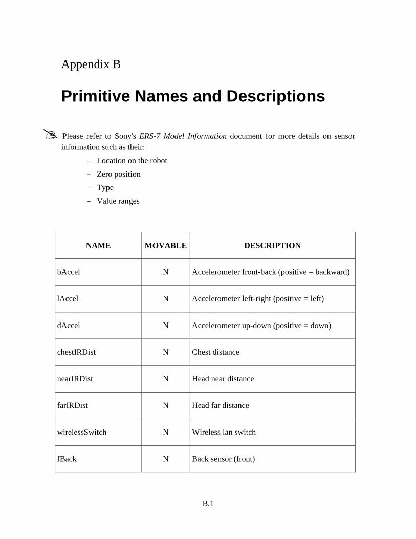
B.1
Appendix B
Primitive Names and Descriptions
� Please refer to Sony's ERS-7 Model Information document for more details on sensor information such as their:
− Location on the robot
− Zero position
− Type
− Value ranges
NAME MOVABLE DESCRIPTION
bAccel N Accelerometer front-back (positive = backward)
lAccel N Accelerometer left-right (positive = left)
dAccel N Accelerometer up-down (positive = down)
chestIRDist N Chest distance
nearIRDist N Head near distance
farIRDist N Head far distance
wirelessSwitch N Wireless lan switch
fBack N Back sensor (front)
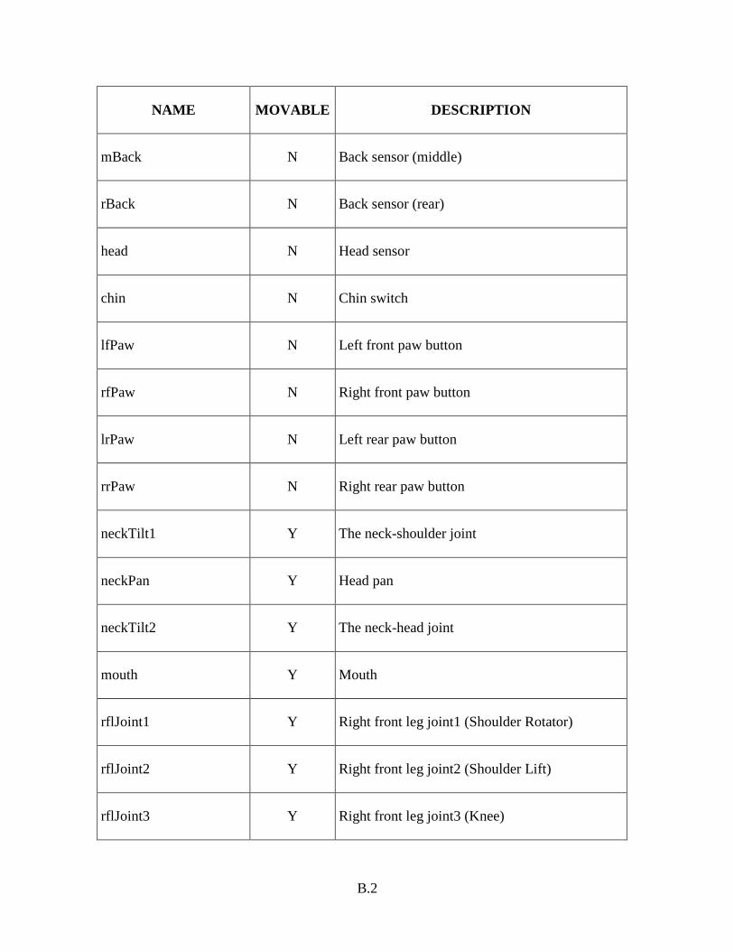
B.2
NAME MOVABLE DESCRIPTION
mBack N Back sensor (middle)
rBack N Back sensor (rear)
head N Head sensor
chin N Chin switch
lfPaw N Left front paw button
rfPaw N Right front paw button
lrPaw N Left rear paw button
rrPaw N Right rear paw button
neckTilt1 Y The neck-shoulder joint
neckPan Y Head pan
neckTilt2 Y The neck-head joint
mouth Y Mouth
rflJoint1 Y Right front leg joint1 (Shoulder Rotator)
rflJoint2 Y Right front leg joint2 (Shoulder Lift)
rflJoint3 Y Right front leg joint3 (Knee)
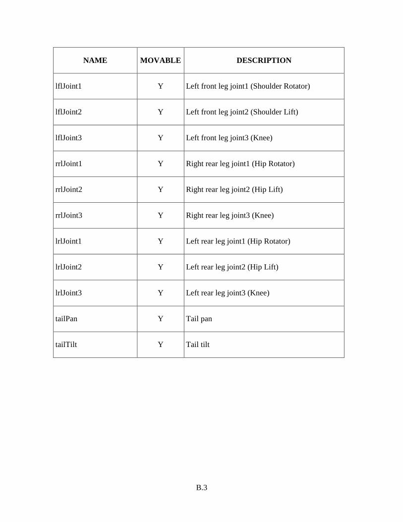
B.3
NAME MOVABLE DESCRIPTION
lflJoint1 Y Left front leg joint1 (Shoulder Rotator)
lflJoint2 Y Left front leg joint2 (Shoulder Lift)
lflJoint3 Y Left front leg joint3 (Knee)
rrlJoint1 Y Right rear leg joint1 (Hip Rotator)
rrlJoint2 Y Right rear leg joint2 (Hip Lift)
rrlJoint3 Y Right rear leg joint3 (Knee)
lrlJoint1 Y Left rear leg joint1 (Hip Rotator)
lrlJoint2 Y Left rear leg joint2 (Hip Lift)
lrlJoint3 Y Left rear leg joint3 (Knee)
tailPan Y Tail pan
tailTilt Y Tail tilt
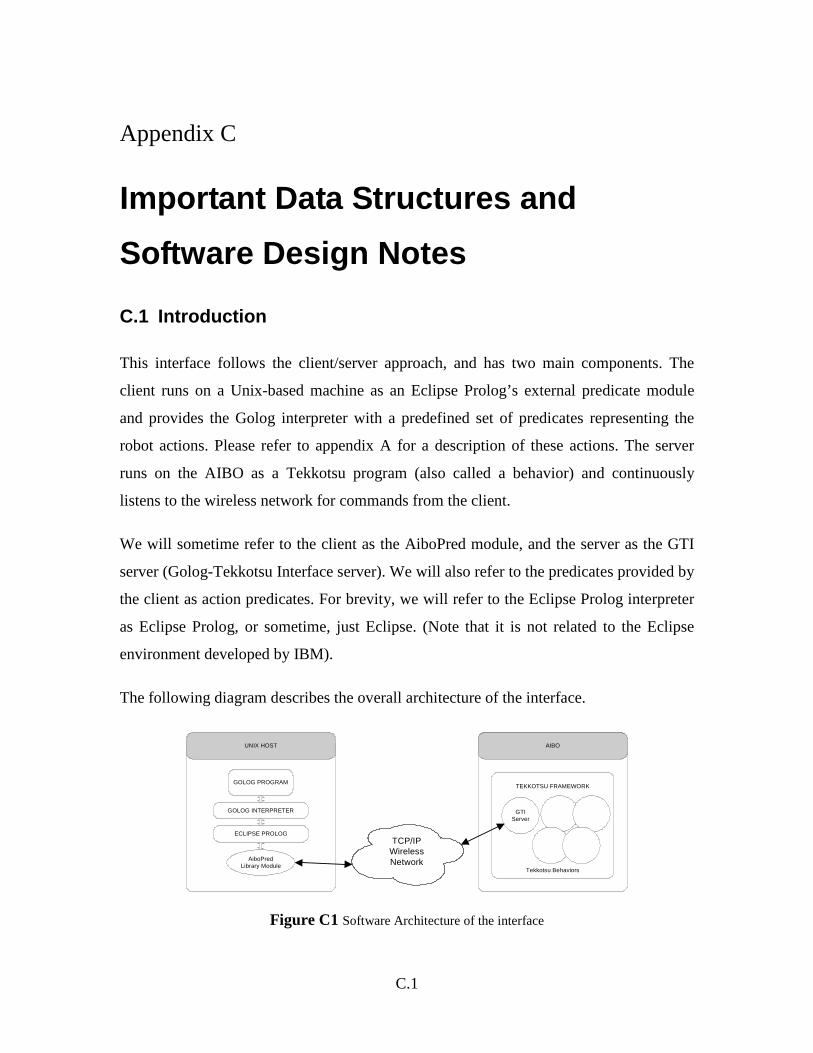
C.1
Appendix C
Important Data Structures and
Software Design Notes
C.1 Introduction
This interface follows the client/server approach, and has two main components. The
client runs on a Unix-based machine as an Eclipse Prolog’s external predicate module
and provides the Golog interpreter with a predefined set of predicates representing the
robot actions. Please refer to appendix A for a description of these actions. The server
runs on the AIBO as a Tekkotsu program (also called a behavior) and continuously
listens to the wireless network for commands from the client.
We will sometime refer to the client as the AiboPred module, and the server as the GTI
server (Golog-Tekkotsu Interface server). We will also refer to the predicates provided by
the client as action predicates. For brevity, we will refer to the Eclipse Prolog interpreter
as Eclipse Prolog, or sometime, just Eclipse. (Note that it is not related to the Eclipse
environment developed by IBM).
The following diagram describes the overall architecture of the interface.
UNIX HOST
ECLIPSE PROLOG
AIBO
TCP/IPWirelessNetworkAiboPred
Library Module
TEKKOTSU FRAMEWORK
GTIServer
Tekkotsu Behaviors
GOLOG INTERPRETER
GOLOG PROGRAM
Figure C1 Software Architecture of the interface
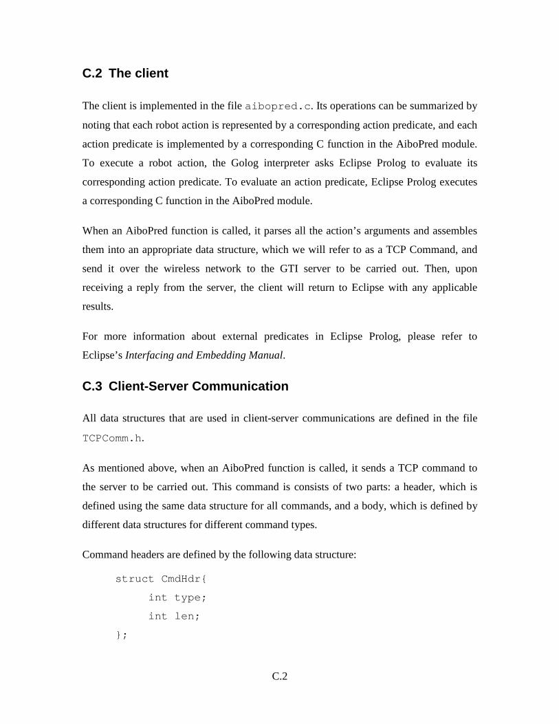
C.2
C.2 The client
The client is implemented in the file aibopred.c. Its operations can be summarized by
noting that each robot action is represented by a corresponding action predicate, and each
action predicate is implemented by a corresponding C function in the AiboPred module.
To execute a robot action, the Golog interpreter asks Eclipse Prolog to evaluate its
corresponding action predicate. To evaluate an action predicate, Eclipse Prolog executes
a corresponding C function in the AiboPred module.
When an AiboPred function is called, it parses all the action’s arguments and assembles
them into an appropriate data structure, which we will refer to as a TCP Command, and
send it over the wireless network to the GTI server to be carried out. Then, upon
receiving a reply from the server, the client will return to Eclipse with any applicable
results.
For more information about external predicates in Eclipse Prolog, please refer to
Eclipse’s Interfacing and Embedding Manual.
C.3 Client-Server Communication
All data structures that are used in client-server communications are defined in the file
TCPComm.h.
As mentioned above, when an AiboPred function is called, it sends a TCP command to
the server to be carried out. This command is consists of two parts: a header, which is
defined using the same data structure for all commands, and a body, which is defined by
different data structures for different command types.
Command headers are defined by the following data structure:
struct CmdHdr{
int type;
int len;
};
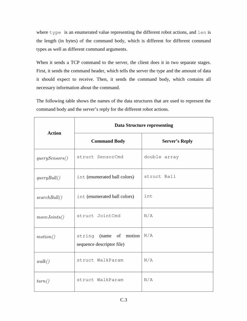
C.3
where type is an enumerated value representing the different robot actions, and len is
the length (in bytes) of the command body, which is different for different command
types as well as different command arguments.
When it sends a TCP command to the server, the client does it in two separate stages.
First, it sends the command header, which tells the server the type and the amount of data
it should expect to receive. Then, it sends the command body, which contains all
necessary information about the command.
The following table shows the names of the data structures that are used to represent the
command body and the server’s reply for the different robot actions.
Data Structure representing
Action
Command Body Server’s Reply
querySensors() struct SensorCmd double array
queryBall() int (enumerated ball colors) struct Ball
searchBall() int (enumerated ball colors) int
moveJoints() struct JointCmd N/A
motion() string (name of motion
sequence descriptor file)
N/A
walk() struct WalkParam N/A
turn() struct WalkParam N/A
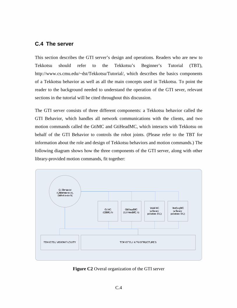
C.4
C.4 The server
This section describes the GTI server’s design and operations. Readers who are new to
Tekkotsu should refer to the Tekkotsu’s Beginner’s Tutorial (TBT),
http://www.cs.cmu.edu/~dst/Tekkotsu/Tutorial/, which describes the basics components
of a Tekkotsu behavior as well as all the main concepts used in Tekkotsu. To point the
reader to the background needed to understand the operation of the GTI sever, relevant
sections in the tutorial will be cited throughout this discussion.
The GTI server consists of three different components: a Tekkotsu behavior called the
GTI Behavior, which handles all network communications with the clients, and two
motion commands called the GtiMC and GtiHeadMC, which interacts with Tekkotsu on
behalf of the GTI Behavior to controls the robot joints. (Please refer to the TBT for
information about the role and design of Tekkotsu behaviors and motion commands.) The
following diagram shows how the three components of the GTI server, along with other
library-provided motion commands, fit together:
Figure C2 Overal organization of the GTI server
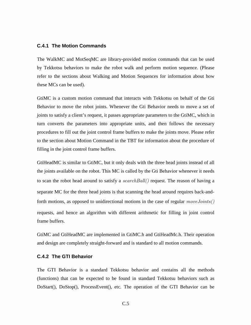
C.5
C.4.1 The Motion Commands
The WalkMC and MotSeqMC are library-provided motion commands that can be used
by Tekkotsu behaviors to make the robot walk and perform motion sequence. (Please
refer to the sections about Walking and Motion Sequences for information about how
these MCs can be used).
GtiMC is a custom motion command that interacts with Tekkotsu on behalf of the Gti
Behavior to move the robot joints. Whenever the Gti Behavior needs to move a set of
joints to satisfy a client’s request, it passes appropriate parameters to the GtiMC, which in
turn converts the parameters into appropriate units, and then follows the necessary
procedures to fill out the joint control frame buffers to make the joints move. Please refer
to the section about Motion Command in the TBT for information about the procedure of
filling in the joint control frame buffers.
GtiHeadMC is similar to GtiMC, but it only deals with the three head joints instead of all
the joints available on the robot. This MC is called by the Gti Behavior whenever it needs
to scan the robot head around to satisfy a searchBall() request. The reason of having a
separate MC for the three head joints is that scanning the head around requires back-and-
forth motions, as opposed to unidirectional motions in the case of regular moveJoints()
requests, and hence an algorithm with different arithmetic for filling in joint control
frame buffers.
GtiMC and GtiHeadMC are implemented in GtiMC.h and GtiHeadMc.h. Their operation
and design are completely straight-forward and is standard to all motion commands.
C.4.2 The GTI Behavior
The GTI Behavior is a standard Tekkotsu behavior and contains all the methods
(functions) that can be expected to be found in standard Tekkotsu behaviors such as
DoStart(), DoStop(), ProcessEvent(), etc. The operation of the GTI Behavior can be
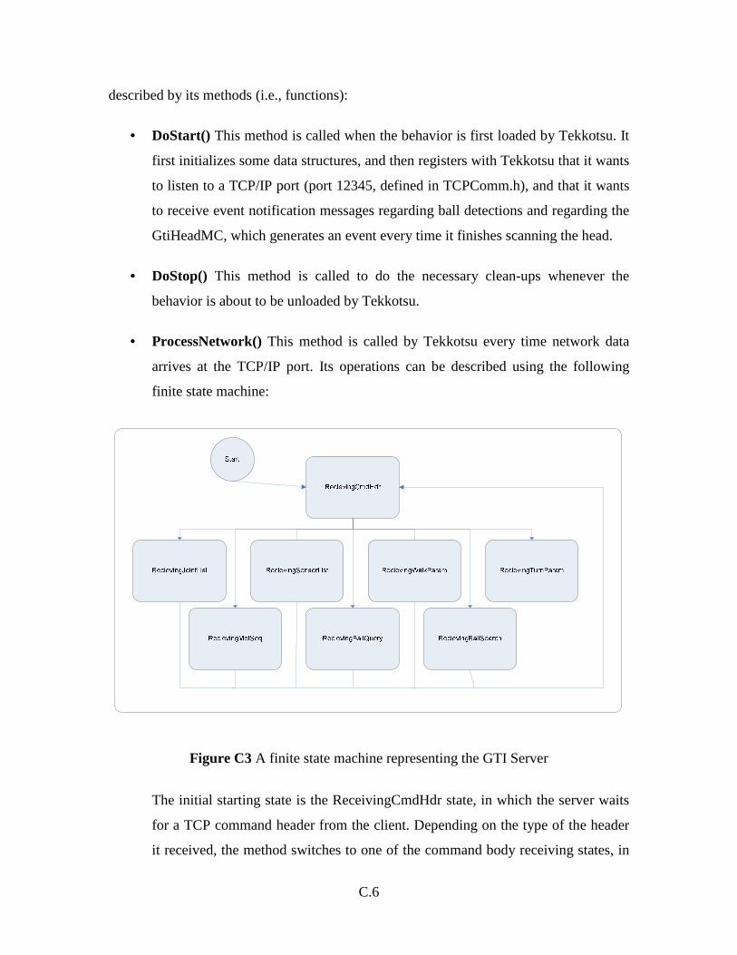
C.6
described by its methods (i.e., functions):
• DoStart() This method is called when the behavior is first loaded by Tekkotsu. It
first initializes some data structures, and then registers with Tekkotsu that it wants
to listen to a TCP/IP port (port 12345, defined in TCPComm.h), and that it wants
to receive event notification messages regarding ball detections and regarding the
GtiHeadMC, which generates an event every time it finishes scanning the head.
• DoStop() This method is called to do the necessary clean-ups whenever the
behavior is about to be unloaded by Tekkotsu.
• ProcessNetwork() This method is called by Tekkotsu every time network data
arrives at the TCP/IP port. Its operations can be described using the following
finite state machine:
Figure C3 A finite state machine representing the GTI Server
The initial starting state is the ReceivingCmdHdr state, in which the server waits
for a TCP command header from the client. Depending on the type of the header
it received, the method switches to one of the command body receiving states, in
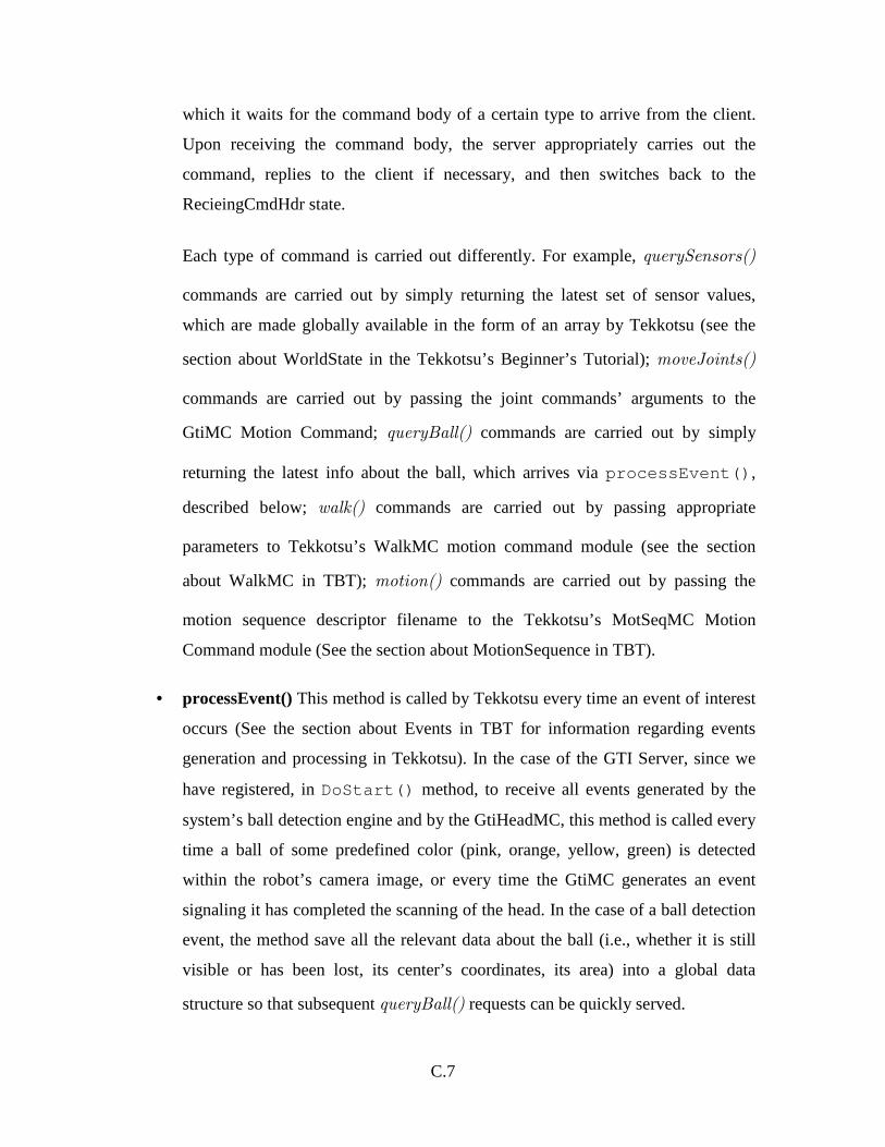
C.7
which it waits for the command body of a certain type to arrive from the client.
Upon receiving the command body, the server appropriately carries out the
command, replies to the client if necessary, and then switches back to the
RecieingCmdHdr state.
Each type of command is carried out differently. For example, querySensors()
commands are carried out by simply returning the latest set of sensor values,
which are made globally available in the form of an array by Tekkotsu (see the
section about WorldState in the Tekkotsu’s Beginner’s Tutorial); moveJoints()
commands are carried out by passing the joint commands’ arguments to the
GtiMC Motion Command; queryBall() commands are carried out by simply
returning the latest info about the ball, which arrives via processEvent(),
described below; walk() commands are carried out by passing appropriate
parameters to Tekkotsu’s WalkMC motion command module (see the section
about WalkMC in TBT); motion() commands are carried out by passing the
motion sequence descriptor filename to the Tekkotsu’s MotSeqMC Motion
Command module (See the section about MotionSequence in TBT).
• processEvent() This method is called by Tekkotsu every time an event of interest
occurs (See the section about Events in TBT for information regarding events
generation and processing in Tekkotsu). In the case of the GTI Server, since we
have registered, in DoStart() method, to receive all events generated by the
system’s ball detection engine and by the GtiHeadMC, this method is called every
time a ball of some predefined color (pink, orange, yellow, green) is detected
within the robot’s camera image, or every time the GtiMC generates an event
signaling it has completed the scanning of the head. In the case of a ball detection
event, the method save all the relevant data about the ball (i.e., whether it is still
visible or has been lost, its center’s coordinates, its area) into a global data
structure so that subsequent queryBall() requests can be quickly served.

C.8
The GTI Behavior is implemented in the file GtiBehavior.h and
GtiBehavior.cc.
The interface source code contains about 2500 lines of code, and an Aibo-ready memory
stick image for this interface, which include Tekkotsu and Open-R’s runtimes modules, is
about 7 MB in size.
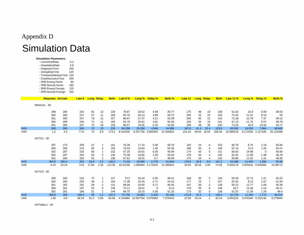
Appendix D
Simulation Data. Simulation Parameters: - CommFailRate 0.2 - HospitalizeRate 0.8 - DiagnosisTime 240 - UnloadingTime 120 - TirednessMarkupTime 120 - CrewRecoveryTime 200 - SPB Emerg Home 80 - SPB Normal Home 160 - SPB Emerg Foreign 120 - SPB Normal Foreign 240
Requests Arrivals Late 8 Long Delay Both Late 8 % Long % Delay % Both % Late 11 Long Delay Both Late 11 % Long % Delay % Both %
MANUAL - 60
298 284 224 81 13 130 78.87 28.52 4.58 45.77 175 48 19 108 61.62 16.9 6.69 38.03300 283 237 57 11 169 83.75 20.14 3.89 59.72 205 32 23 150 72.44 11.31 8.13 53301 285 247 78 12 157 86.67 27.37 4.21 55.09 206 45 21 140 72.28 15.79 7.37 49.12300 289 245 74 11 160 84.78 25.61 3.81 55.36 194 34 19 141 67.13 11.76 6.57 48.79301 284 247 70 18 159 86.97 24.65 6.34 55.99 208 48 30 130 73.24 16.9 10.56 45.77
AVG 300 285 240 72 13 155 84.208 25.258 4.566 54.386 197.6 41.4 22.4 133.8 69.342 14.532 7.864 46.942VAR 1.2 4.4 77.6 70 6.8 173.2 8.544256 8.357736 0.860504 21.340824 151.44 48.64 16.64 206.56 19.589216 6.172536 2.127184 25.131096
AUTO1 - 60
297 274 209 47 1 161 76.28 17.15 0.36 58.76 183 24 6 153 66.79 8.76 2.19 55.84300 280 214 55 4 155 76.43 19.64 1.43 55.36 188 35 4 149 67.14 12.5 1.43 53.21302 287 193 60 1 132 67.25 20.91 0.35 45.99 174 43 0 131 60.63 14.98 0 45.64303 287 202 54 3 145 70.38 18.82 1.05 50.52 178 34 4 140 62.02 11.85 1.39 48.78301 284 192 52 2 138 67.61 18.31 0.7 48.59 170 33 4 133 59.86 11.62 1.41 46.83
AVG 300.6 282.4 202 53.6 2.2 146.2 71.59 18.966 0.778 51.844 178.6 33.8 3.6 141.2 63.288 11.942 1.284 50.06VAR 4.24 24.24 74.8 17.84 1.36 113.36 16.31236 1.596584 0.172616 21.360824 40.64 36.56 3.84 74.56 9.505176 3.955616 0.503584 14.98772
AUTO2 - 60
299 283 210 72 1 137 74.2 25.44 0.35 48.41 168 36 4 128 59.36 12.72 1.41 45.23302 283 202 46 2 154 71.38 16.25 0.71 54.42 177 23 7 147 62.54 8.13 2.47 51.94301 282 192 59 2 131 68.09 20.92 0.71 46.45 167 36 3 128 59.22 12.77 1.06 45.39300 281 197 52 0 145 70.11 18.51 0 51.6 179 35 6 138 63.7 12.46 2.14 49.11302 281 196 51 1 144 69.75 18.15 0.36 51.25 173 32 5 136 61.57 11.39 1.78 48.4
AVG 300.8 282 199.4 56 1.2 142.2 70.706 19.854 0.426 50.426 172.8 32.4 5 135.4 61.278 11.494 1.772 48.014VAR 1.36 0.8 38.24 81.2 0.56 60.56 4.154984 10.007704 0.070584 7.576424 22.56 24.24 2 50.24 3.091616 3.078344 0.252136 6.279944
OPTIMAL1 - 60
D.1
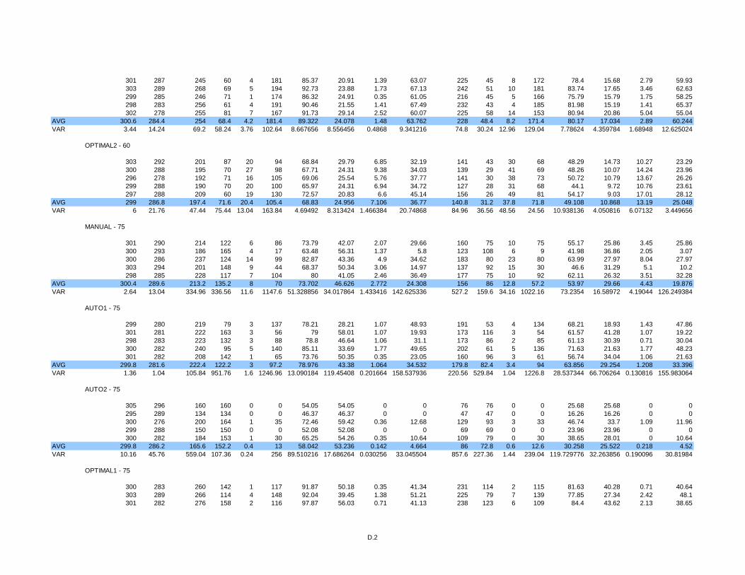
301 287 245 60 4 181 85.37 20.91 1.39 63.07 225 45 8 172 78.4 15.68 2.79 59.93303 289 268 69 5 194 92.73 23.88 1.73 67.13 242 51 10 181 83.74 17.65 3.46 62.63299 285 246 71 1 174 86.32 24.91 0.35 61.05 216 45 5 166 75.79 15.79 1.75 58.25298 283 256 61 4 191 90.46 21.55 1.41 67.49 232 43 4 185 81.98 15.19 1.41 65.37302 278 255 81 7 167 91.73 29.14 2.52 60.07 225 58 14 153 80.94 20.86 5.04 55.04
AVG 300.6 284.4 254 68.4 4.2 181.4 89.322 24.078 1.48 63.762 228 48.4 8.2 171.4 80.17 17.034 2.89 60.244VAR 3.44 14.24 69.2 58.24 3.76 102.64 8.667656 8.556456 0.4868 9.341216 74.8 30.24 12.96 129.04 7.78624 4.359784 1.68948 12.625024
OPTIMAL2 - 60
303 292 201 87 20 94 68.84 29.79 6.85 32.19 141 43 30 68 48.29 14.73 10.27 23.29300 288 195 70 27 98 67.71 24.31 9.38 34.03 139 29 41 69 48.26 10.07 14.24 23.96296 278 192 71 16 105 69.06 25.54 5.76 37.77 141 30 38 73 50.72 10.79 13.67 26.26299 288 190 70 20 100 65.97 24.31 6.94 34.72 127 28 31 68 44.1 9.72 10.76 23.61297 288 209 60 19 130 72.57 20.83 6.6 45.14 156 26 49 81 54.17 9.03 17.01 28.12
AVG 299 286.8 197.4 71.6 20.4 105.4 68.83 24.956 7.106 36.77 140.8 31.2 37.8 71.8 49.108 10.868 13.19 25.048VAR 6 21.76 47.44 75.44 13.04 163.84 4.69492 8.313424 1.466384 20.74868 84.96 36.56 48.56 24.56 10.938136 4.050816 6.07132 3.449656
MANUAL - 75
301 290 214 122 6 86 73.79 42.07 2.07 29.66 160 75 10 75 55.17 25.86 3.45 25.86300 293 186 165 4 17 63.48 56.31 1.37 5.8 123 108 6 9 41.98 36.86 2.05 3.07300 286 237 124 14 99 82.87 43.36 4.9 34.62 183 80 23 80 63.99 27.97 8.04 27.97303 294 201 148 9 44 68.37 50.34 3.06 14.97 137 92 15 30 46.6 31.29 5.1 10.2298 285 228 117 7 104 80 41.05 2.46 36.49 177 75 10 92 62.11 26.32 3.51 32.28
AVG 300.4 289.6 213.2 135.2 8 70 73.702 46.626 2.772 24.308 156 86 12.8 57.2 53.97 29.66 4.43 19.876VAR 2.64 13.04 334.96 336.56 11.6 1147.6 51.328856 34.017864 1.433416 142.625336 527.2 159.6 34.16 1022.16 73.2354 16.58972 4.19044 126.249384
AUTO1 - 75
299 280 219 79 3 137 78.21 28.21 1.07 48.93 191 53 4 134 68.21 18.93 1.43 47.86301 281 222 163 3 56 79 58.01 1.07 19.93 173 116 3 54 61.57 41.28 1.07 19.22298 283 223 132 3 88 78.8 46.64 1.06 31.1 173 86 2 85 61.13 30.39 0.71 30.04300 282 240 95 5 140 85.11 33.69 1.77 49.65 202 61 5 136 71.63 21.63 1.77 48.23301 282 208 142 1 65 73.76 50.35 0.35 23.05 160 96 3 61 56.74 34.04 1.06 21.63
AVG 299.8 281.6 222.4 122.2 3 97.2 78.976 43.38 1.064 34.532 179.8 82.4 3.4 94 63.856 29.254 1.208 33.396VAR 1.36 1.04 105.84 951.76 1.6 1246.96 13.090184 119.45408 0.201664 158.537936 220.56 529.84 1.04 1226.8 28.537344 66.706264 0.130816 155.983064
AUTO2 - 75
305 296 160 160 0 0 54.05 54.05 0 0 76 76 0 0 25.68 25.68 0 0295 289 134 134 0 0 46.37 46.37 0 0 47 47 0 0 16.26 16.26 0 0300 276 200 164 1 35 72.46 59.42 0.36 12.68 129 93 3 33 46.74 33.7 1.09 11.96299 288 150 150 0 0 52.08 52.08 0 0 69 69 0 0 23.96 23.96 0 0300 282 184 153 1 30 65.25 54.26 0.35 10.64 109 79 0 30 38.65 28.01 0 10.64
AVG 299.8 286.2 165.6 152.2 0.4 13 58.042 53.236 0.142 4.664 86 72.8 0.6 12.6 30.258 25.522 0.218 4.52VAR 10.16 45.76 559.04 107.36 0.24 256 89.510216 17.686264 0.030256 33.045504 857.6 227.36 1.44 239.04 119.729776 32.263856 0.190096 30.81984
OPTIMAL1 - 75
300 283 260 142 1 117 91.87 50.18 0.35 41.34 231 114 2 115 81.63 40.28 0.71 40.64303 289 266 114 4 148 92.04 39.45 1.38 51.21 225 79 7 139 77.85 27.34 2.42 48.1301 282 276 158 2 116 97.87 56.03 0.71 41.13 238 123 6 109 84.4 43.62 2.13 38.65
D.2
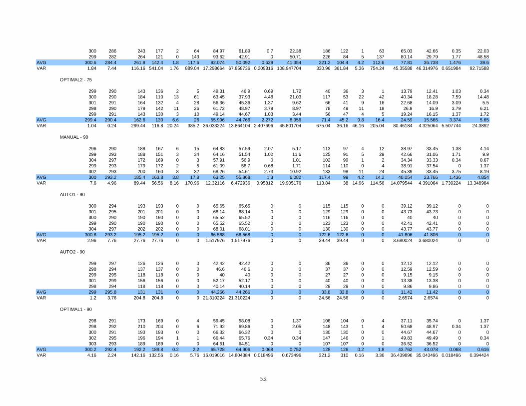
300 286 243 177 2 64 84.97 61.89 0.7 22.38 186 122 1 63 65.03 42.66 0.35 22.03299 282 264 121 0 143 93.62 42.91 0 50.71 226 84 5 137 80.14 29.79 1.77 48.58
AVG 300.6 284.4 261.8 142.4 1.8 117.6 92.074 50.092 0.628 41.354 221.2 104.4 4.2 112.6 77.81 36.738 1.476 39.6VAR 1.84 7.44 116.16 541.04 1.76 889.04 17.298664 67.858736 0.209816 108.947704 330.96 361.84 5.36 754.24 45.35588 46.314976 0.651984 92.71588
OPTIMAL2 - 75
299 290 143 136 2 5 49.31 46.9 0.69 1.72 40 36 3 1 13.79 12.41 1.03 0.34300 290 184 110 13 61 63.45 37.93 4.48 21.03 117 53 22 42 40.34 18.28 7.59 14.48301 291 164 132 4 28 56.36 45.36 1.37 9.62 66 41 9 16 22.68 14.09 3.09 5.5298 290 179 142 11 26 61.72 48.97 3.79 8.97 78 49 11 18 26.9 16.9 3.79 6.21299 291 143 130 3 10 49.14 44.67 1.03 3.44 56 47 4 5 19.24 16.15 1.37 1.72
AVG 299.4 290.4 162.6 130 6.6 26 55.996 44.766 2.272 8.956 71.4 45.2 9.8 16.4 24.59 15.566 3.374 5.65VAR 1.04 0.24 299.44 116.8 20.24 385.2 36.033224 13.864104 2.407696 45.801704 675.04 36.16 46.16 205.04 80.46184 4.325064 5.507744 24.3892
MANUAL - 90
296 290 188 167 6 15 64.83 57.59 2.07 5.17 113 97 4 12 38.97 33.45 1.38 4.14299 293 188 151 3 34 64.16 51.54 1.02 11.6 125 91 5 29 42.66 31.06 1.71 9.9304 297 172 169 0 3 57.91 56.9 0 1.01 102 99 1 2 34.34 33.33 0.34 0.67299 293 179 172 2 5 61.09 58.7 0.68 1.71 114 110 0 4 38.91 37.54 0 1.37302 293 200 160 8 32 68.26 54.61 2.73 10.92 133 98 11 24 45.39 33.45 3.75 8.19
AVG 300 293.2 185.4 163.8 3.8 17.8 63.25 55.868 1.3 6.082 117.4 99 4.2 14.2 40.054 33.766 1.436 4.854VAR 7.6 4.96 89.44 56.56 8.16 170.96 12.32116 6.472936 0.95812 19.905176 113.84 38 14.96 114.56 14.079544 4.391064 1.739224 13.348984
AUTO1 - 90
300 294 193 193 0 0 65.65 65.65 0 0 115 115 0 0 39.12 39.12 0 0301 295 201 201 0 0 68.14 68.14 0 0 129 129 0 0 43.73 43.73 0 0300 290 190 190 0 0 65.52 65.52 0 0 116 116 0 0 40 40 0 0299 290 190 190 0 0 65.52 65.52 0 0 123 123 0 0 42.41 42.41 0 0304 297 202 202 0 0 68.01 68.01 0 0 130 130 0 0 43.77 43.77 0 0
AVG 300.8 293.2 195.2 195.2 0 0 66.568 66.568 0 0 122.6 122.6 0 0 41.806 41.806 0 0VAR 2.96 7.76 27.76 27.76 0 0 1.517976 1.517976 0 0 39.44 39.44 0 0 3.680024 3.680024 0 0
AUTO2 - 90
299 297 126 126 0 0 42.42 42.42 0 0 36 36 0 0 12.12 12.12 0 0298 294 137 137 0 0 46.6 46.6 0 0 37 37 0 0 12.59 12.59 0 0299 295 118 118 0 0 40 40 0 0 27 27 0 0 9.15 9.15 0 0301 299 156 156 0 0 52.17 52.17 0 0 40 40 0 0 13.38 13.38 0 0298 294 118 118 0 0 40.14 40.14 0 0 29 29 0 0 9.86 9.86 0 0
AVG 299 295.8 131 131 0 0 44.266 44.266 0 0 33.8 33.8 0 0 11.42 11.42 0 0VAR 1.2 3.76 204.8 204.8 0 0 21.310224 21.310224 0 0 24.56 24.56 0 0 2.6574 2.6574 0 0
OPTIMAL1 - 90
298 291 173 169 0 4 59.45 58.08 0 1.37 108 104 0 4 37.11 35.74 0 1.37298 292 210 204 0 6 71.92 69.86 0 2.05 148 143 1 4 50.68 48.97 0.34 1.37300 291 193 193 0 0 66.32 66.32 0 0 130 130 0 0 44.67 44.67 0 0302 295 196 194 1 1 66.44 65.76 0.34 0.34 147 146 0 1 49.83 49.49 0 0.34303 293 189 189 0 0 64.51 64.51 0 0 107 107 0 0 36.52 36.52 0 0
AVG 300.2 292.4 192.2 189.8 0.2 2.2 65.728 64.906 0.068 0.752 128 126 0.2 1.8 43.762 43.078 0.068 0.616VAR 4.16 2.24 142.16 132.56 0.16 5.76 16.019016 14.804384 0.018496 0.673496 321.2 310 0.16 3.36 36.439896 35.043496 0.018496 0.394424
D.3
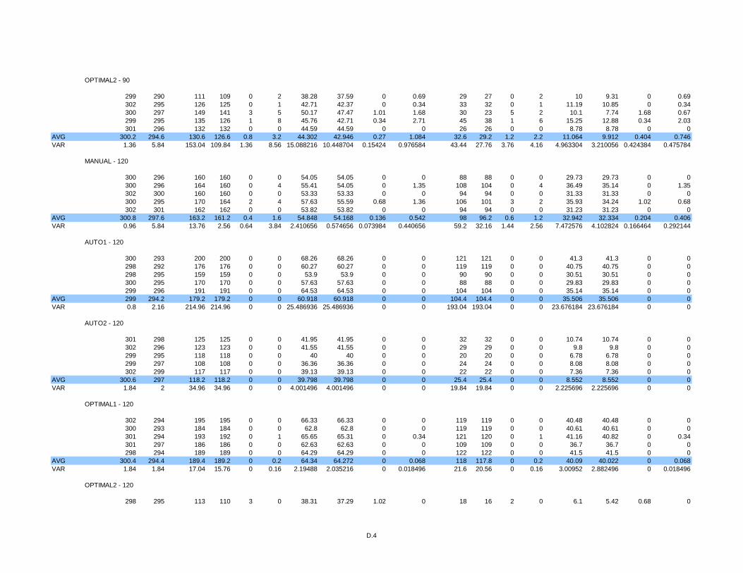
OPTIMAL2 - 90
299 290 111 109 0 2 38.28 37.59 0 0.69 29 27 0 2 10 9.31 0 0.69302 295 126 125 0 1 42.71 42.37 0 0.34 33 32 0 1 11.19 10.85 0 0.34300 297 149 141 3 5 50.17 47.47 1.01 1.68 30 23 5 2 10.1 7.74 1.68 0.67299 295 135 126 1 8 45.76 42.71 0.34 2.71 45 38 1 6 15.25 12.88 0.34 2.03301 296 132 132 0 0 44.59 44.59 0 0 26 26 0 0 8.78 8.78 0 0
AVG 300.2 294.6 130.6 126.6 0.8 3.2 44.302 42.946 0.27 1.084 32.6 29.2 1.2 2.2 11.064 9.912 0.404 0.746VAR 1.36 5.84 153.04 109.84 1.36 8.56 15.088216 10.448704 0.15424 0.976584 43.44 27.76 3.76 4.16 4.963304 3.210056 0.424384 0.475784
MANUAL - 120
300 296 160 160 0 0 54.05 54.05 0 0 88 88 0 0 29.73 29.73 0 0300 296 164 160 0 4 55.41 54.05 0 1.35 108 104 0 4 36.49 35.14 0 1.35302 300 160 160 0 0 53.33 53.33 0 0 94 94 0 0 31.33 31.33 0 0300 295 170 164 2 4 57.63 55.59 0.68 1.36 106 101 3 2 35.93 34.24 1.02 0.68302 301 162 162 0 0 53.82 53.82 0 0 94 94 0 0 31.23 31.23 0 0
AVG 300.8 297.6 163.2 161.2 0.4 1.6 54.848 54.168 0.136 0.542 98 96.2 0.6 1.2 32.942 32.334 0.204 0.406VAR 0.96 5.84 13.76 2.56 0.64 3.84 2.410656 0.574656 0.073984 0.440656 59.2 32.16 1.44 2.56 7.472576 4.102824 0.166464 0.292144
AUTO1 - 120
300 293 200 200 0 0 68.26 68.26 0 0 121 121 0 0 41.3 41.3 0 0298 292 176 176 0 0 60.27 60.27 0 0 119 119 0 0 40.75 40.75 0 0298 295 159 159 0 0 53.9 53.9 0 0 90 90 0 0 30.51 30.51 0 0300 295 170 170 0 0 57.63 57.63 0 0 88 88 0 0 29.83 29.83 0 0299 296 191 191 0 0 64.53 64.53 0 0 104 104 0 0 35.14 35.14 0 0
AVG 299 294.2 179.2 179.2 0 0 60.918 60.918 0 0 104.4 104.4 0 0 35.506 35.506 0 0VAR 0.8 2.16 214.96 214.96 0 0 25.486936 25.486936 0 0 193.04 193.04 0 0 23.676184 23.676184 0 0
AUTO2 - 120
301 298 125 125 0 0 41.95 41.95 0 0 32 32 0 0 10.74 10.74 0 0302 296 123 123 0 0 41.55 41.55 0 0 29 29 0 0 9.8 9.8 0 0299 295 118 118 0 0 40 40 0 0 20 20 0 0 6.78 6.78 0 0299 297 108 108 0 0 36.36 36.36 0 0 24 24 0 0 8.08 8.08 0 0302 299 117 117 0 0 39.13 39.13 0 0 22 22 0 0 7.36 7.36 0 0
AVG 300.6 297 118.2 118.2 0 0 39.798 39.798 0 0 25.4 25.4 0 0 8.552 8.552 0 0VAR 1.84 2 34.96 34.96 0 0 4.001496 4.001496 0 0 19.84 19.84 0 0 2.225696 2.225696 0 0
OPTIMAL1 - 120
302 294 195 195 0 0 66.33 66.33 0 0 119 119 0 0 40.48 40.48 0 0300 293 184 184 0 0 62.8 62.8 0 0 119 119 0 0 40.61 40.61 0 0301 294 193 192 0 1 65.65 65.31 0 0.34 121 120 0 1 41.16 40.82 0 0.34301 297 186 186 0 0 62.63 62.63 0 0 109 109 0 0 36.7 36.7 0 0298 294 189 189 0 0 64.29 64.29 0 0 122 122 0 0 41.5 41.5 0 0
AVG 300.4 294.4 189.4 189.2 0 0.2 64.34 64.272 0 0.068 118 117.8 0 0.2 40.09 40.022 0 0.068VAR 1.84 1.84 17.04 15.76 0 0.16 2.19488 2.035216 0 0.018496 21.6 20.56 0 0.16 3.00952 2.882496 0 0.018496
OPTIMAL2 - 120
298 295 113 110 3 0 38.31 37.29 1.02 0 18 16 2 0 6.1 5.42 0.68 0
D.4
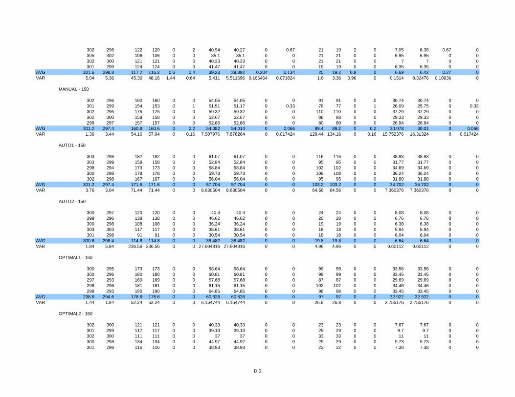
302 298 122 120 0 2 40.94 40.27 0 0.67 21 19 2 0 7.05 6.38 0.67 0305 302 106 106 0 0 35.1 35.1 0 0 21 21 0 0 6.95 6.95 0 0302 300 121 121 0 0 40.33 40.33 0 0 21 21 0 0 7 7 0 0301 299 124 124 0 0 41.47 41.47 0 0 19 19 0 0 6.35 6.35 0 0
AVG 301.6 298.8 117.2 116.2 0.6 0.4 39.23 38.892 0.204 0.134 20 19.2 0.8 0 6.69 6.42 0.27 0VAR 5.04 5.36 45.36 48.16 1.44 0.64 5.411 5.511696 0.166464 0.071824 1.6 3.36 0.96 0 0.1514 0.32476 0.10936 0
MANUAL - 150
302 296 160 160 0 0 54.05 54.05 0 0 91 91 0 0 30.74 30.74 0 0301 299 154 153 0 1 51.51 51.17 0 0.33 78 77 0 1 26.09 25.75 0 0.33302 295 175 175 0 0 59.32 59.32 0 0 110 110 0 0 37.29 37.29 0 0302 300 158 158 0 0 52.67 52.67 0 0 88 88 0 0 29.33 29.33 0 0299 297 157 157 0 0 52.86 52.86 0 0 80 80 0 0 26.94 26.94 0 0
AVG 301.2 297.4 160.8 160.6 0 0.2 54.082 54.014 0 0.066 89.4 89.2 0 0.2 30.078 30.01 0 0.066VAR 1.36 3.44 54.16 57.04 0 0.16 7.507976 7.876264 0 0.017424 129.44 134.16 0 0.16 15.752376 16.31324 0 0.017424
AUTO1 - 150
303 298 182 182 0 0 61.07 61.07 0 0 116 116 0 0 38.93 38.93 0 0303 299 158 158 0 0 52.84 52.84 0 0 95 95 0 0 31.77 31.77 0 0298 294 173 173 0 0 58.84 58.84 0 0 102 102 0 0 34.69 34.69 0 0300 298 178 178 0 0 59.73 59.73 0 0 108 108 0 0 36.24 36.24 0 0302 298 167 167 0 0 56.04 56.04 0 0 95 95 0 0 31.88 31.88 0 0
AVG 301.2 297.4 171.6 171.6 0 0 57.704 57.704 0 0 103.2 103.2 0 0 34.702 34.702 0 0VAR 3.76 3.04 71.44 71.44 0 0 8.630504 8.630504 0 0 64.56 64.56 0 0 7.360376 7.360376 0 0
AUTO2 - 150
300 297 120 120 0 0 40.4 40.4 0 0 24 24 0 0 8.08 8.08 0 0299 296 138 138 0 0 46.62 46.62 0 0 20 20 0 0 6.76 6.76 0 0300 298 108 108 0 0 36.24 36.24 0 0 19 19 0 0 6.38 6.38 0 0303 303 117 117 0 0 38.61 38.61 0 0 18 18 0 0 5.94 5.94 0 0301 298 91 91 0 0 30.54 30.54 0 0 18 18 0 0 6.04 6.04 0 0
AVG 300.6 298.4 114.8 114.8 0 0 38.482 38.482 0 0 19.8 19.8 0 0 6.64 6.64 0 0VAR 1.84 5.84 236.56 236.56 0 0 27.604816 27.604816 0 0 4.96 4.96 0 0 0.60112 0.60112 0 0
OPTIMAL1 - 150
300 295 173 173 0 0 58.64 58.64 0 0 99 99 0 0 33.56 33.56 0 0300 296 180 180 0 0 60.81 60.81 0 0 99 99 0 0 33.45 33.45 0 0297 293 169 169 0 0 57.68 57.68 0 0 87 87 0 0 29.69 29.69 0 0298 296 181 181 0 0 61.15 61.15 0 0 102 102 0 0 34.46 34.46 0 0298 293 190 190 0 0 64.85 64.85 0 0 98 98 0 0 33.45 33.45 0 0
AVG 298.6 294.6 178.6 178.6 0 0 60.626 60.626 0 0 97 97 0 0 32.922 32.922 0 0VAR 1.44 1.84 52.24 52.24 0 0 6.154744 6.154744 0 0 26.8 26.8 0 0 2.755176 2.755176 0 0
OPTIMAL2 - 150
302 300 121 121 0 0 40.33 40.33 0 0 23 23 0 0 7.67 7.67 0 0301 299 117 117 0 0 39.13 39.13 0 0 29 29 0 0 9.7 9.7 0 0302 300 111 111 0 0 37 37 0 0 33 33 0 0 11 11 0 0300 298 134 134 0 0 44.97 44.97 0 0 29 29 0 0 9.73 9.73 0 0301 298 116 116 0 0 38.93 38.93 0 0 22 22 0 0 7.38 7.38 0 0
D.5
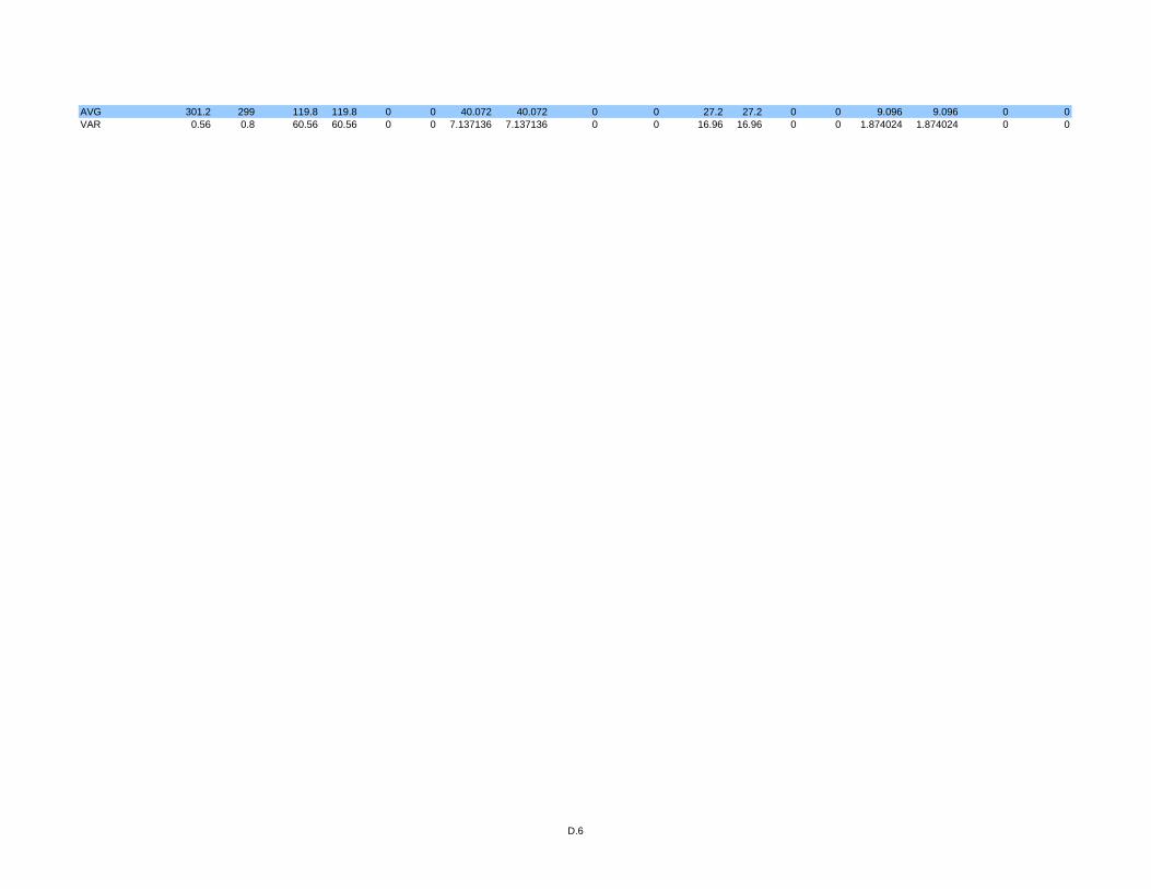
AVG 301.2 299 119.8 119.8 0 0 40.072 40.072 0 0 27.2 27.2 0 0 9.096 9.096 0 0VAR 0.56 0.8 60.56 60.56 0 0 7.137136 7.137136 0 0 16.96 16.96 0 0 1.874024 1.874024 0 0
D.6
90
References
[1] D. Andre, "Programmable reinforcement learning agents." PhD Thesis. Computer Science Division, University of California, Berkeley. Available at http://205.201.13.117/davidandre/diss.html 2003.
[2] A. Barto, S. Bradtke, and S. Singh, "Learning to Act using Real-Time Dynamic Programming," In Artificial Intelligence, vol. 72, pp. 81-138, 1995.
[3] C. Boutilier, T. Dean, and S. Hanks, "Decision-Theoretic Planning: Structural Assumptions and Computational Leverage," Journal of Artificial Intelligence Research, vol. 11, pp. 1-94, 1999.
[4] C. Boutilier, R. Reiter, and B. Price, "Symbolic Dynamic Programming for First-order MDPs," Proceedings of the Seventeenth International Joint Conference on Artificial Intelligence, 2001.
[5] N. Cole and P. Stone, "Machine Learning for Fast Quadrupedal Locomotion," Proceedings of the Nineteenth National Conference on Artificial Intelligence AAAI-04, 2004.
[6] N. Cole and P. Stone, "Policy Gradient Reinforcement Learning for Fast Quadrupedal Locomotion," 2004.
[7] CommDirectorate, "Report of the Inquiry Into The London Ambulance Service (South West Thames Regional Health Authority)" "The 8th International Workshop on Software Specification and Design Case Study. Electronic Version prepared by Anthony Finkelstein. Available at http://www.cs.ucl.ac.uk/staff/A.Finkelstein/las.html", 1993.
[8] Crabbe Frederick, "Unifying Undergraduate Artificial Intelligence Robotics: Layers of Abstraction Over Two Channels," Artificial Intelligence Magazine, pp. 23-38, 2006.
[9] T. Dietterich, "Hierarchical Reinforcement Learning with the MAXQ Value Function Decomposition," Journal of Artificial Intelligence Research, vol. 13, pp. 227-303, 2000.
[10] A. Ferrein, Fritz C, and G. Lakemeyer, "Using Golog for Deliberation and Team Coordination in Robotic Soccer," KI Künstliche Intelligenz, vol. 1 2005.
91
[11] C. Fritz, "Integrating decision-theoretic planning and programming for robot control in highly dynamic domains." Masters Thesis. RWTH-Aachen, Germany. Available at http://www.cs.toronto.edu/~fritz/ 2003.
[12] C. Fritz and S. McIlraith, "Decision-Theoretic GOLOG with Qualitative Preferences," Proceedings of the 10th International Conference on Principles of Knowledge Representation and Reasoning, Lake District, UK, 2006.
[13] J. Kramer and A. Wolf, "Succeedings of the 8th International Workshop on Software Specification and Design," ACM SIGSOFT Software Engineering Notes, vol. 21, no. 5, pp. 21-35, 1996.
[14] E. Letier and A. Lamsweerde, "Reasoning about partial goal satisfaction for requirements and design engineering," Proceedings of the 12th ACM SIGSOFT International Symposium on Foundations of Software Engineering, pp. 53-62, 2004.
[15] J. McCarthy and P. Hayes, "Some philosophical problems from the standpoint of artificial intelligence," Machine Intelligence, pp. 463-502, 1969.
[16] R. Parr, "Hierarchical control and learning for markov decision processes." PhD Thesis. Computer Science Division, University of California, Berkeley. Available at http://www.cs.duke.edu/~parr/#papers 1998.
[17] L. Peret and F. Garcia, "On-Line Search for Solving Markov Decision Processes via Heuristic Sampling," Proceedings of the 16th Eureopean Conference on Artificial Intelligence, ECAI2004, pp. 530-534, 2004.
[18] R. Reiter, Knowledge in Action: Logical Foundations for Specifying and Implementing Dynamical Systems MIT Press, 2001.
[19] S. Sanner and C. Boutilier, "Practical linear value-approximation techniques for first-order MDPs," In Proceedings of the 22nd Conference on Uncertainty in AI (UAI-06), 2006.
[20] M. Shriharan, G. Kuhlmann, and P. Stone, "Practical Vision-Based Monte Carlo Localization on a Legged Robot," Proceedings of the IEEE International Conference on Robotics and Automation, 2005.
[21] M. Shriharan and P. Stone, "Real-Time Vision on a Mobile Robot Platform," Proceedings of the IEEE International Conference on Intelligent Robots and Systems, 2005.
[22] V. Soni and S. Singh, "Reinforcement Learning of Hierarchical Skills on the Sony Aibo robot," AAAI Technical Report Series, 2005.
92
[23] M. Soutchanski, "An On-line Decision-Theoretic Golog Interpreter," in Proceedings of the Seventeenth International Conference on Artificial Intelligence (IJCAI-01) 2001, pp. 19-26.
[24] M. Soutchanski, "High-level robot programming in dynamic and incompletely known environments." PhD Thesis. Department of Computer Science, University of Toronto. Available at http://www.scs.ryerson.ca/~mes/publications/ 2003.
[25] M. Soutchanski, H. Pham, and J. Mylopoulos, "Decision making in large-scale domains: a case study," A Members Poster in the American Association for Artificial Intelligence Conference, 2006.
[26] M. Soutchanski, H. Pham, and J. Mylopoulos, "Decision Making in Uncertain Real-World Domains Using DT-Golog," The European Conference on AI (ECAI-06), 2006.
[27] P. Stone, R. S. Sutton, and G. Krulmann, "Reinforcement Learning for RoboCup-Soccer Keepaway," Adaptive Behavior, vol. 13, no. 3, pp. 165-188, 2005.
[28] R. Sutton, D. Precup, and S. Singh, "Between MDPs and Semi-MDPs: A Framework for Temporal Abstraction in Reinforcement Learning," Artif. Intell., vol. 112, pp. 181-211, 1999.
[29] M. Veloso, W. Uther, M. Fujita, M. Asada, and H. Kitano, "Playing soccer with legged robots," In Proceedings of the Intelligent Robots and Systems Conference, 1998.
[30] M. Veloso, E. Winner, S. Lenser, J. Bruce, and T. Balch, "Vision-Servoed Localization and Behavior-Based Planning for an Autonomous Quadruped Legged Robot," Proceedings of the International Conference on Artificial Intelligence Planning Systems, 2000.
[31] J. You, "Applying the GRL Framework to the LAS-CAD Case Study," Technical Report. University of Toronto.,2004.