Embed Size (px)
Citation preview

Applying Computational Methods to Determinethe Electric Current Density in a MHD GeneratorChannel from External Flux Density Measurements
V. A. Bokil1, N. L. Gibson1, D. A. McGregor1,2, C. R. Woodside2
(1) Oregon State University(2)National Energy Technology Laboratory
Pacific Coast Carbon Storage / Computational Energy Science ResearchCloseout Meeting
October 29, 2014
Gibson (OSU) ACMDECDMHDGCEFDM NETL 2014 1 / 11
Finding Arcs in MHD Generators
V. A. Bokil1, N. L. Gibson1, D. A. McGregor1,2, C. R. Woodside2
(1) Oregon State University(2)National Energy Technology Laboratory
Pacific Coast Carbon Storage / Computational Energy Science ResearchCloseout Meeting
October 29, 2014
Gibson (OSU) Finding Arcs in MHD Generators NETL 2014 1 / 29

Outline
1 Introduction
2 Inverse Problem
3 Modeling
4 Simulation
5 Sensitivity Analysis
6 Conclusions
Gibson (OSU) Finding Arcs in MHD Generators NETL 2014 2 / 29

Outline
1 Introduction
2 Inverse Problem
3 Modeling
4 Simulation
5 Sensitivity Analysis
6 Conclusions
Gibson (OSU) Finding Arcs in MHD Generators NETL 2014 2 / 29

Outline
1 Introduction
2 Inverse Problem
3 Modeling
4 Simulation
5 Sensitivity Analysis
6 Conclusions
Gibson (OSU) Finding Arcs in MHD Generators NETL 2014 2 / 29

Outline
1 Introduction
2 Inverse Problem
3 Modeling
4 Simulation
5 Sensitivity Analysis
6 Conclusions
Gibson (OSU) Finding Arcs in MHD Generators NETL 2014 2 / 29
Outline
1 Introduction
2 Inverse Problem
3 Modeling
4 Simulation
5 Sensitivity Analysis
6 Conclusions
Gibson (OSU) Finding Arcs in MHD Generators NETL 2014 2 / 29

Outline
1 Introduction
2 Inverse Problem
3 Modeling
4 Simulation
5 Sensitivity Analysis
6 Conclusions
Gibson (OSU) Finding Arcs in MHD Generators NETL 2014 2 / 29

Introduction
Outline
1 Introduction
2 Inverse Problem
3 Modeling
4 Simulation
5 Sensitivity Analysis
6 Conclusions
Gibson (OSU) Finding Arcs in MHD Generators NETL 2014 3 / 29
Introduction
Magneto-hydrodynamic Power Generation
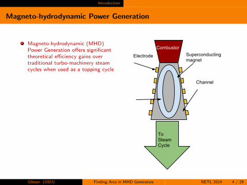
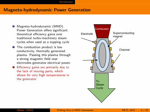
Magneto-hydrodynamic (MHD)Power Generation offers significanttheoretical efficiency gains overtraditional turbo-machinery steamcycles when used as a topping cycle
The combustion product is lowconductivity, thermally generatedplasma. Passing this plasma througha strong magnetic field nearelectrodes generates electrical power.
However, MHD Power Generationsuffers from high life-cycle costs due,in part, to high component failurerates inside the channel, potentiallycaused by “arcing”.
Combustor
To Steam Cycle
Electrode Superconducting magnet
Channel
Gibson (OSU) Finding Arcs in MHD Generators NETL 2014 4 / 29
Introduction
Magneto-hydrodynamic Power Generation
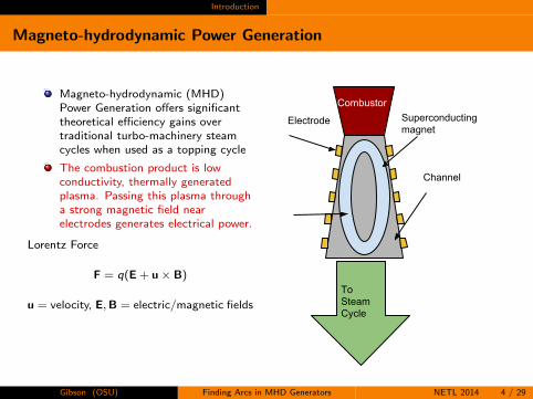
Magneto-hydrodynamic (MHD)Power Generation offers significanttheoretical efficiency gains overtraditional turbo-machinery steamcycles when used as a topping cycle
The combustion product is lowconductivity, thermally generatedplasma. Passing this plasma througha strong magnetic field nearelectrodes generates electrical power.
Lorentz Force
F = q(E + u× B)
u = velocity, E,B = electric/magnetic fields
However, MHD Power Generationsuffers from high life-cycle costs due,in part, to high component failurerates inside the channel, potentiallycaused by “arcing”.
Combustor
To Steam Cycle
Electrode Superconducting magnet
Channel
Gibson (OSU) Finding Arcs in MHD Generators NETL 2014 4 / 29
Introduction
Magneto-hydrodynamic Power Generation
Magneto-hydrodynamic (MHD)Power Generation offers significanttheoretical efficiency gains overtraditional turbo-machinery steamcycles when used as a topping cycle
The combustion product is lowconductivity, thermally generatedplasma. Passing this plasma througha strong magnetic field nearelectrodes generates electrical power.
Efficiency gains are primarily due tothe lack of moving parts, whichallows for very high temperatures inthe generator.
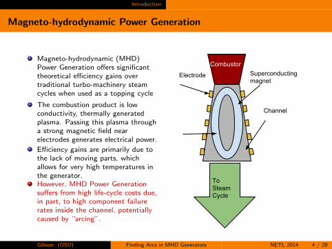
However, MHD Power Generationsuffers from high life-cycle costs due,in part, to high component failurerates inside the channel, potentiallycaused by “arcing”.
Combustor
To Steam Cycle
Electrode Superconducting magnet
Channel
Gibson (OSU) Finding Arcs in MHD Generators NETL 2014 4 / 29
Introduction
Magneto-hydrodynamic Power Generation
Magneto-hydrodynamic (MHD)Power Generation offers significanttheoretical efficiency gains overtraditional turbo-machinery steamcycles when used as a topping cycle
The combustion product is lowconductivity, thermally generatedplasma. Passing this plasma througha strong magnetic field nearelectrodes generates electrical power.
Efficiency gains are primarily due tothe lack of moving parts, whichallows for very high temperatures inthe generator.However, MHD Power Generationsuffers from high life-cycle costs due,in part, to high component failurerates inside the channel, potentiallycaused by “arcing”.
Combustor
To Steam Cycle
Electrode Superconducting magnet
Channel
Gibson (OSU) Finding Arcs in MHD Generators NETL 2014 4 / 29

Introduction
MHD Generator Arcs
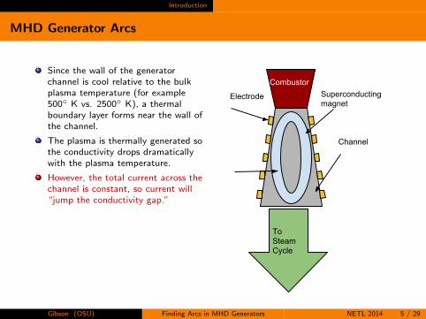
Since the wall of the generatorchannel is cool relative to the bulkplasma temperature (for example500◦ K vs. 2500◦ K), a thermalboundary layer forms near the wall ofthe channel.
The plasma is thermally generated sothe conductivity drops dramaticallywith the plasma temperature.
However, the total current across thechannel is constant, so current will“jump the conductivity gap.”
It does so in very high density arcs.These arcs are hot and damage theelectrodes, which must be replaced.
We seek to detect the location ofarcs (areas of particularly largecurrent density) from externalmagnetic flux density measurements.
Combustor
To Steam Cycle
Electrode Superconducting magnet
Channel
Gibson (OSU) Finding Arcs in MHD Generators NETL 2014 5 / 29

Introduction
MHD Generator Arcs
Since the wall of the generatorchannel is cool relative to the bulkplasma temperature (for example500◦ K vs. 2500◦ K), a thermalboundary layer forms near the wall ofthe channel.
The plasma is thermally generated sothe conductivity drops dramaticallywith the plasma temperature.
However, the total current across thechannel is constant, so current will“jump the conductivity gap.”
It does so in very high density arcs.These arcs are hot and damage theelectrodes, which must be replaced.
We seek to detect the location ofarcs (areas of particularly largecurrent density) from externalmagnetic flux density measurements.
Combustor
To Steam Cycle
Electrode Superconducting magnet
Channel
Gibson (OSU) Finding Arcs in MHD Generators NETL 2014 5 / 29
Introduction
MHD Generator Arcs
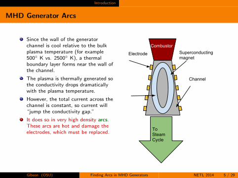
Since the wall of the generatorchannel is cool relative to the bulkplasma temperature (for example500◦ K vs. 2500◦ K), a thermalboundary layer forms near the wall ofthe channel.
The plasma is thermally generated sothe conductivity drops dramaticallywith the plasma temperature.
However, the total current across thechannel is constant, so current will“jump the conductivity gap.”
It does so in very high density arcs.These arcs are hot and damage theelectrodes, which must be replaced.
We seek to detect the location ofarcs (areas of particularly largecurrent density) from externalmagnetic flux density measurements.
Combustor
To Steam Cycle
Electrode Superconducting magnet
Channel
Gibson (OSU) Finding Arcs in MHD Generators NETL 2014 5 / 29

Introduction
MHD Generator Arcs
Since the wall of the generatorchannel is cool relative to the bulkplasma temperature (for example500◦ K vs. 2500◦ K), a thermalboundary layer forms near the wall ofthe channel.
The plasma is thermally generated sothe conductivity drops dramaticallywith the plasma temperature.
However, the total current across thechannel is constant, so current will“jump the conductivity gap.”
It does so in very high density arcs.These arcs are hot and damage theelectrodes, which must be replaced.
We seek to detect the location ofarcs (areas of particularly largecurrent density) from externalmagnetic flux density measurements.
Combustor
To Steam Cycle
Electrode Superconducting magnet
Channel
Gibson (OSU) Finding Arcs in MHD Generators NETL 2014 5 / 29

Inverse Problem
Outline
1 Introduction
2 Inverse Problem
3 Modeling
4 Simulation
5 Sensitivity Analysis
6 Conclusions
Gibson (OSU) Finding Arcs in MHD Generators NETL 2014 6 / 29
Inverse Problem
Reconstruction
Current densities inside the generator cannot be directly measureddue to high temperatures, magnetic fields, and corrosive gasses
There is, however, a magnetic field that is induced by the internalelectric field, which extends beyond the channel
Measuring internal features by induced magnetic fields has beensuccessfully implemented for Vacuum Arc Remelters
We are interested in Current Reconstruction using externalmeasurements of the induced magnetic flux density
Typically current reconstruction relies on the solution of integralequations, e.g., the Biot-Savart Law [1, 2], which involves specialassumptions of geometry and/or material parameters
Instead, we solve a more flexible differential equations model andperform a simulation-based parameter estimation.
Gibson (OSU) Finding Arcs in MHD Generators NETL 2014 7 / 29
Inverse Problem
Simulation-Based Parameter Estimation
We assume a parameterization of the quantity of interest(current density)
Given external field measurements, we find the minimizer of adiscrepancy function involving a simulation(using Newton’s method to explore parameter space)
Requires no special assumptions of geometry or material
In practice, convergence depends on accuracy of initial estimates
Need an accurate model of the essential physics, and an efficientnumerical simulation method
Gibson (OSU) Finding Arcs in MHD Generators NETL 2014 8 / 29

Inverse Problem
Non-linear Least Squares
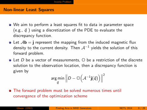
We aim to perform a least squares fit to data in parameter space(e.g., ~q ) using a discretization of the PDE to evaluate thediscrepancy function.
Let Ab = j represent the mapping from the induced magnetic fluxdensity to the current density. Then A−1 yields the solution of thisforward problem.
Let D be a vector of measurements, O be a restriction of the discretesolution to the observation location, then a discrepancy function isgiven by
arg min~q
∥∥∥D −O(A−1j(~q)
)∥∥∥2
The forward problem must be solved numerous times untilconvergence of the optimization scheme
Gibson (OSU) Finding Arcs in MHD Generators NETL 2014 9 / 29

Inverse Problem
Non-linear Least Squares
We aim to perform a least squares fit to data in parameter space(e.g., ~q ) using a discretization of the PDE to evaluate thediscrepancy function.
Let Ab = j represent the mapping from the induced magnetic fluxdensity to the current density. Then A−1 yields the solution of thisforward problem.
Let D be a vector of measurements, O be a restriction of the discretesolution to the observation location, then a discrepancy function isgiven by
arg min~q
∥∥∥D −O(A−1j(~q)
)∥∥∥2
The forward problem must be solved numerous times untilconvergence of the optimization scheme
Gibson (OSU) Finding Arcs in MHD Generators NETL 2014 9 / 29

Modeling
Outline
1 Introduction
2 Inverse Problem
3 Modeling
4 Simulation
5 Sensitivity Analysis
6 Conclusions
Gibson (OSU) Finding Arcs in MHD Generators NETL 2014 10 / 29
Modeling Bulk MHD Equations
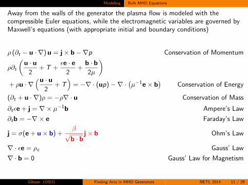
Away from the walls of the generator the plasma flow is modeled with thecompressible Euler equations, while the electromagnetic variables are governed byMaxwell’s equations (with appropriate initial and boundary conditions)
ρ (∂t − u · ∇) u = j× b−∇p Conservation of Momentum
ρ∂t
(u · u
2+ T +
εe · e2
+b · b2µ
)+ ρu · ∇
(u · u2
+ T)
= −∇ · (up)−∇ ·(µ−1e× b
)Conservation of Energy
(∂t + u · ∇)ρ = −ρ∇ · u Conservation of Mass
∂tεe + j = ∇× µ−1b Ampere’s Law
∂tb = −∇× e Faraday’s Law
j = σ(e + u× b) +β√b · b
j× b Ohm’s Law
∇ · εe = ρc Gauss’ Law
∇ · b = 0 Gauss’ Law for Magnetism
Gibson (OSU) Finding Arcs in MHD Generators NETL 2014 11 / 29
Modeling Bulk MHD Equations
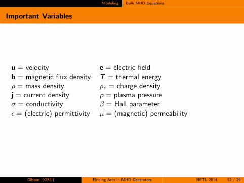
Important Variables
u = velocity e = electric fieldb = magnetic flux density T = thermal energyρ = mass density ρc = charge densityj = current density p = plasma pressureσ = conductivity β = Hall parameterε = (electric) permittivity µ = (magnetic) permeability
Gibson (OSU) Finding Arcs in MHD Generators NETL 2014 12 / 29
Modeling Bulk MHD Equations
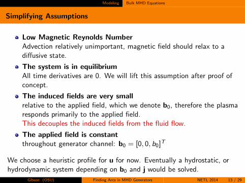
Simplifying Assumptions
Low Magnetic Reynolds NumberAdvection relatively unimportant, magnetic field should relax to adiffusive state.
The system is in equilibriumAll time derivatives are 0. We will lift this assumption after proof ofconcept.
The induced fields are very smallrelative to the applied field, which we denote b0, therefore the plasmaresponds primarily to the applied field.This decouples the induced fields from the fluid flow.
The applied field is constantthroughout generator channel: b0 = [0, 0, b0]T
We choose a heuristic profile for u for now. Eventually a hydrostatic, orhydrodynamic system depending on b0 and j would be solved.
Gibson (OSU) Finding Arcs in MHD Generators NETL 2014 13 / 29
Modeling Bulk MHD Equations
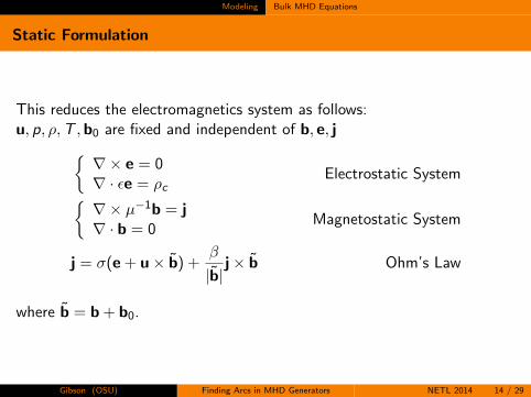
Static Formulation
This reduces the electromagnetics system as follows:u, p, ρ,T ,b0 are fixed and independent of b, e, j{
∇× e = 0∇ · εe = ρc
Electrostatic System{∇× µ−1b = j∇ · b = 0
Magnetostatic System
j = σ(e + u× b) +β
|b|j× b Ohm’s Law
where b = b + b0.
Gibson (OSU) Finding Arcs in MHD Generators NETL 2014 14 / 29

Modeling Bulk MHD Equations
Magnetostatic Problem
We formulate the magnetostatic problem in Coloumb Gauge:∇ · b = 0 =⇒ b = ∇× a, where a is the magnetic (vector) potential. Wechoose ∇ · a = 0.
∇× µ−1∇× a = j
∇ · a = 0
However when we formulate the variational problem, we enforce thedivergence condition weakly. Find (a, λ) ∈ H∇× × H1.{
(∇× a,∇× c)L2 + (∇λ, c)L2 = (j, c)L2
(a,∇η)L2 = 0∀(c, η) ∈ H∇× × H1 (∗)
This problem is a well posed saddle point system. Further if ∇ · j = 0then λ = 0.
Weak divergence imposes less regularity on a and also requires fewerdegrees of freedom. [3].
Gibson (OSU) Finding Arcs in MHD Generators NETL 2014 15 / 29
Modeling Bulk MHD Equations
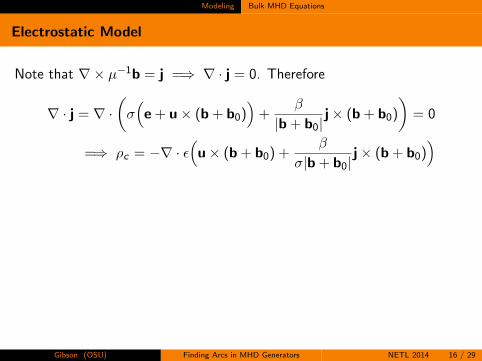
Electrostatic Model
Note that ∇× µ−1b = j =⇒ ∇ · j = 0. Therefore
∇ · j = ∇ ·(σ(
e + u× (b + b0))
+β
|b + b0|j× (b + b0)
)= 0
=⇒ ρc = −∇ · ε(
u× (b + b0) +β
σ|b + b0|j× (b + b0)
)
By Helmholtz decomposition, as ∇× e = 0 then e = ∇ψ, where ψ is theelectric (scalar) potential. Using the above consistency condition we havethe following electrostatic problem.
−∇ · ε∇ψ = ∇ · ε(
u× (b + b0) +β
σ|b + b0|j× (b + b0)
)(∗∗)
Gibson (OSU) Finding Arcs in MHD Generators NETL 2014 16 / 29

Modeling Bulk MHD Equations
Electrostatic Model
Note that ∇× µ−1b = j =⇒ ∇ · j = 0. Therefore
∇ · j = ∇ ·(σ(
e + u× (b + b0))
+β
|b + b0|j× (b + b0)
)= 0
=⇒ ρc = −∇ · ε(
u× (b + b0) +β
σ|b + b0|j× (b + b0)
)
By Helmholtz decomposition, as ∇× e = 0 then e = ∇ψ, where ψ is theelectric (scalar) potential. Using the above consistency condition we havethe following electrostatic problem.
−∇ · ε∇ψ = ∇ · ε(
u× (b + b0) +β
σ|b + b0|j× (b + b0)
)(∗∗)
Gibson (OSU) Finding Arcs in MHD Generators NETL 2014 16 / 29

Simulation
Outline
1 Introduction
2 Inverse Problem
3 Modeling
4 Simulation
5 Sensitivity Analysis
6 Conclusions
Gibson (OSU) Finding Arcs in MHD Generators NETL 2014 17 / 29
Simulation
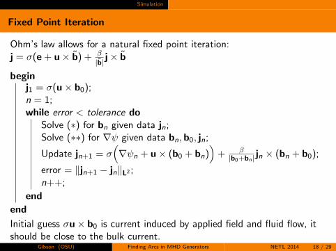
Fixed Point Iteration
Ohm’s law allows for a natural fixed point iteration:j = σ(e + u× b) + β
|b| j× b
beginj1 = σ(u× b0);n = 1;while error < tolerance do
Solve (∗) for bn given data jn;Solve (∗∗) for ∇ψ given data bn,b0, jn;
Update jn+1 = σ(∇ψn + u× (b0 + bn)
)+ β|b0+bn| jn × (bn + b0);
error = ‖jn+1 − jn‖L2 ;n++;
end
end
Initial guess σu× b0 is current induced by applied field and fluid flow, itshould be close to the bulk current.
Gibson (OSU) Finding Arcs in MHD Generators NETL 2014 18 / 29

Simulation
Magnetostatic Solver (M)
Electrostatic Solver (E)
Ohm’s Law Fixed Point Iteration (O)
Electro-Magnetic System Iterates until convergence
Hydrostatic Solve (H)
Magnetic Flux Density (b)Electric Field (e)Current Density (j)Plasma Velocity (u)
Initial Guess (G)
Fluid Mechanics System iterates until convergence
(M): Takes data j and and produces induced magnetic flux density b using Ampere’s Law and Gauss’ Law for Magnetism
(E): Takes data j,u, and b and produces electric field e using Faraday’s Law and Gauss’ Law
(O): Takes data j, b, e, u to produce new current estimate j using Ohm’s Law
(H): Takes data b and j to produce plasma velocity u using Navier-Stokes Equations and Lorentz Force
(G): An initial guess j and u
Gibson (OSU) Finding Arcs in MHD Generators NETL 2014 19 / 29
Simulation
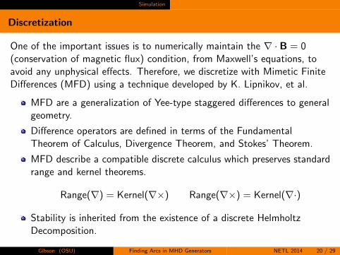
Discretization
One of the important issues is to numerically maintain the ∇ · B = 0(conservation of magnetic flux) condition, from Maxwell’s equations, toavoid any unphysical effects. Therefore, we discretize with Mimetic FiniteDifferences (MFD) using a technique developed by K. Lipnikov, et al.
MFD are a generalization of Yee-type staggered differences to generalgeometry.
Difference operators are defined in terms of the FundamentalTheorem of Calculus, Divergence Theorem, and Stokes’ Theorem.
MFD describe a compatible discrete calculus which preserves standardrange and kernel theorems.
Range(∇) = Kernel(∇×) Range(∇×) = Kernel(∇·)
Stability is inherited from the existence of a discrete HelmholtzDecomposition.
Gibson (OSU) Finding Arcs in MHD Generators NETL 2014 20 / 29

Simulation
Discretizations of Interest
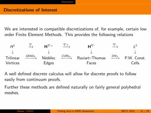
We are interested in compatible discretizations of, for example, certain loworder Finite Element Methods. This provides the following relations
H1 ∇−→ H∇×∇×−−→ H∇·
∇·−→ L2
↓ ↓ ↓ ↓Trilinear
GRADh−−−−→ NedelecCURLh−−−−→ Raviart–Thomas
DIVh−−−→ P.W. Const.Vertices Edges Faces Cells
A well defined discrete calculus will allow for discrete proofs to followeasily from continuum proofs.
Further these methods are defined naturally on fairly general polyhedralmeshes.
Gibson (OSU) Finding Arcs in MHD Generators NETL 2014 21 / 29

Simulation
Discretizations of Interest
We are interested in compatible discretizations of, for example, certain loworder Finite Element Methods. This provides the following relations
H1 ∇−→ H∇×∇×−−→ H∇·
∇·−→ L2
↓ ↓ ↓ ↓Trilinear
GRADh−−−−→ NedelecCURLh−−−−→ Raviart–Thomas
DIVh−−−→ P.W. Const.Vertices Edges Faces Cells
A well defined discrete calculus will allow for discrete proofs to followeasily from continuum proofs.
Further these methods are defined naturally on fairly general polyhedralmeshes.
Gibson (OSU) Finding Arcs in MHD Generators NETL 2014 21 / 29
Simulation
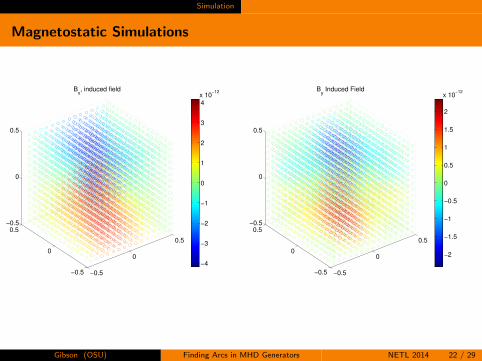
Magnetostatic Simulations
−0.5
0
0.5
−0.5
0
0.5−0.5
0
0.5
Bx, induced field
−4
−3
−2
−1
0
1
2
3
4
x 10−12
−0.5
0
0.5
−0.5
0
0.5−0.5
0
0.5
By Induced Field
−2
−1.5
−1
−0.5
0
0.5
1
1.5
2
x 10−12
Gibson (OSU) Finding Arcs in MHD Generators NETL 2014 22 / 29

Sensitivity Analysis
Outline
1 Introduction
2 Inverse Problem
3 Modeling
4 Simulation
5 Sensitivity Analysis
6 Conclusions
Gibson (OSU) Finding Arcs in MHD Generators NETL 2014 23 / 29

Sensitivity Analysis
Features of the Arc
There are several features of an arc which we wish to be able to detectand quantify. In order to determine the feasibility of a simulation-basedparameter estimation, we first test the sensitivity of the measurementsto
jm: Total current in the system
θ: Tilting of the current due to the Hall effect
s: (Spread of) the distribution of current density.
We assume a parameterized current density profile j which has thesefeatures:
j(x , y , z ; jm, θ, s) =jm√2πs2
v exp
1
2s2
∣∣∣∣∣∣(I− vvT )
xyz
∣∣∣∣∣∣2 , v =
cos θsin θ
0
Gibson (OSU) Finding Arcs in MHD Generators NETL 2014 24 / 29

Sensitivity Analysis
Sensitivity Results
0 0.2 0.4 0.6 0.8 1−2.5
−2
−1.5
−1
−0.5
0
0.5
1
1.5
2
2.5x 10⁻⁷
Standard Deviation of Current Profile (m)
Indu
ced
Mag
netic
Flu
x D
ensi
ty (
T)
Jm
= 106, θ=π/2−.1
Bx(0,0,0)
Bx(0,.25,0)
By(0,0,0)
By(0,.25,0)
0.7 0.8 0.9 1 1.1 1.2 1.3 1.4 1.5 1.6−8
−6
−4
−2
0
2
4
6
8x 10
−7J
m=106, s=1/16, h=1/32
Current Tilt Parameter θ (rad)
Indu
ced
Mag
entic
Flu
x D
ensi
ty (
T)
Bx(0,0,0)
Bx(0,.25,0)
By(0,0,0)
By(0,.25,0)
Gibson (OSU) Finding Arcs in MHD Generators NETL 2014 25 / 29

Conclusions
Outline
1 Introduction
2 Inverse Problem
3 Modeling
4 Simulation
5 Sensitivity Analysis
6 Conclusions
Gibson (OSU) Finding Arcs in MHD Generators NETL 2014 26 / 29
Conclusions
Conclusions
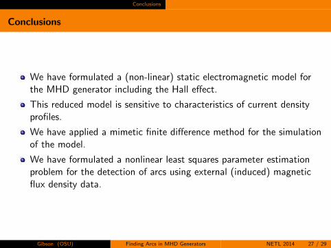
We have formulated a (non-linear) static electromagnetic model forthe MHD generator including the Hall effect.
This reduced model is sensitive to characteristics of current densityprofiles.
We have applied a mimetic finite difference method for the simulationof the model.
We have formulated a nonlinear least squares parameter estimationproblem for the detection of arcs using external (induced) magneticflux density data.
Gibson (OSU) Finding Arcs in MHD Generators NETL 2014 27 / 29
Conclusions
Future Work
Solve the inverse problem for the reduced model.
Include quantification of uncertainty in measurements and estimation.
Simulate the full (dynamic, coupled) forward problem.
Solve the full inverse problem.
Gibson (OSU) Finding Arcs in MHD Generators NETL 2014 28 / 29
Conclusions
References
[1] K. Hauer and R. Potthast.
Magnetic tomography for fuel cells- current status and problems.
J.Phys.:Conf. Ser. 73 012008, pages 1–17, 2008.
[2] R. Kress, L. Kuhn, and R. Potthast.
Reconstruction of a current distribution from its magnetic field.
Inv. Prob., 18:1127–1146, 2002.
[3] K. Lipnikov, G. Manzini, F. Brezzi, and A. Buff.
The mimetic finite difference method for the 3d magnetostatic field problemson polyhedral meshes.
J. Comp. Phys., 230:305–328, 2011.
[4] Richard Rosa.
Magnetohydrodynamic energy conversion.
McGraw-Hill, 1968.
Gibson (OSU) Finding Arcs in MHD Generators NETL 2014 29 / 29