ORIGINAL RESEARCH ARTICLEpublished: 04 February 2015

doi: 10.3389/fncom.2015.00008

Applying artificial vision models to human sceneunderstandingElissa M. Aminoff1,2*, Mariya Toneva1,3, Abhinav Shrivastava4, Xinlei Chen4, Ishan Misra4,

Abhinav Gupta4 and Michael J. Tarr1,2

1 Center for the Neural Basis of Cognition, Carnegie Mellon University, Pittsburgh, PA, USA2 Department of Psychology, Carnegie Mellon University, Pittsburgh, PA, USA3 Department of Machine Learning, Carnegie Mellon University, Pittsburgh, PA, USA4 Robotics Institute, Carnegie Mellon University, Pittsburgh, PA, USA

Edited by:

Hans P. Op De Beeck, University ofLeuven, Belgium

Reviewed by:

Dwight Kravitz, National Institutes ofHealth, USASean MacEvoy, Boston College,USA

*Correspondence:

Elissa M. Aminoff, Department ofPsychology, Carnegie MellonUniversity, 352 Baker Hall, 5000Forbes Ave., Pittsburgh, PA 15213,USAe-mail: eaminoff@cmu.edu

How do we understand the complex patterns of neural responses that underlie sceneunderstanding? Studies of the network of brain regions held to be scene-selective—theparahippocampal/lingual region (PPA), the retrosplenial complex (RSC), and the occipitalplace area (TOS)—have typically focused on single visual dimensions (e.g., size), ratherthan the high-dimensional feature space in which scenes are likely to be neurallyrepresented. Here we leverage well-specified artificial vision systems to explicate amore complex understanding of how scenes are encoded in this functional network.We correlated similarity matrices within three different scene-spaces arising from: (1)BOLD activity in scene-selective brain regions; (2) behavioral measured judgments ofvisually-perceived scene similarity; and (3) several different computer vision models.These correlations revealed: (1) models that relied on mid- and high-level sceneattributes showed the highest correlations with the patterns of neural activity withinthe scene-selective network; (2) NEIL and SUN—the models that best accounted forthe patterns obtained from PPA and TOS—were different from the GIST model thatbest accounted for the pattern obtained from RSC; (3) The best performing modelsoutperformed behaviorally-measured judgments of scene similarity in accounting forneural data. One computer vision method—NEIL (“Never-Ending-Image-Learner”), whichincorporates visual features learned as statistical regularities across web-scale numbersof scenes—showed significant correlations with neural activity in all three scene-selectiveregions and was one of the two models best able to account for variance in the PPAand TOS. We suggest that these results are a promising first step in explicating morefine-grained models of neural scene understanding, including developing a clearer pictureof the division of labor among the components of the functional scene-selective brainnetwork.

Keywords: scene processing, parahippocampal place area, retrosplenial cortex, transverse occipital sulcus,

computer vision

INTRODUCTIONThe past several decades have given us an unprecedented view ofthe inner workings of the human brain, allowing us to measurelocalized neural activity in awake, behaving humans. As cognitiveneuroscientists, our challenge is to make sense of this rich sourceof data, connecting the activity we observe to mental mechanismsand behavior. For those of us who study high-level vision, makingthis connection is particularly difficult—vision scientists have notyet articulated any clear theories about what constitutes a “vocab-ulary” of intermediate visual features or what are the underlyingbuilding blocks of scene or object representation. Here we beginto address this issue by taking a different path to articulating acandidate set of features for visual representation: using a varietyof extant computer vision models that make different commit-ments as to what counts as a visual feature as proxies for models

of biological vision. We suggest that, to the extent that computervision models and biological vision systems have similar endgoals, the two domains will overlap in both their representationsand processing assumptions.

To explore this issue, we had participants view 100 differ-ent scenes while we measured their brain activity, using func-tional Magnetic Resonance Imaging (“fMRI”), in regions that areknown to be preferentially involved in scene processing. In partic-ular, we hold that meaningful information can be extracted fromthe reliable patterns of activity that occur within scene selectiveregions: the parahippocampal/lingual region (the parahippocam-pal place area, “PPA”), the retrosplenial complex (“RSC”), and theoccipital place area (also referred to as the transverse occipital sul-cus, “TOS”). However, due to a lack of any fine-grained theoriesof scene understanding, it is unclear as to how one goes about

Frontiers in Computational Neuroscience www.frontiersin.org February 2015 | Volume 9 | Article 8 | 1

COMPUTATIONAL NEUROSCIENCE

Aminoff et al. Scene-space in PPA, RSC, TOS

interpreting the complex meaning inherent in these neural pat-terns. As alluded to above, we turn to models of computer visionto help us unravel how the human brain encodes and representsvisual scenes, directly comparing the representations of sceneswithin these artificial vision systems to our obtained patterns ofBOLD activity as measured by fMRI. The application of modelsderived from computer vision has one significant advantage: themodels are well specified. As such, any particular model makesclear and explicit assumptions regarding representation and cor-respondence between a model and human neural responses orbehavior allows us to infer that the two work similarly. Henceour emphasis on comparing a large number of models that allwork somewhat differently from one another. In adopting mod-ern computer vision models, we also note that these systemsare built to understand the same complex visual world we dealwith everyday (i.e., in contrast to earlier models that relied on“toy” worlds or highly-restricted visual domains). In particular,some of the models we include leverage large-scale/“web-scale”image datasets that may more accurately learn informative visualregularities embedded in the natural environment.

In that we have no strong a priori knowledge as to which ofseveral very different models might be most effective with respectto accounting for neural data, our primary goal is to test whetherwe observe some correspondence between the patterns of neuralactivity elicited in high-order visual scene regions (i.e., PPA, RSC,and TOS) and the patterns of scene similarity as defined by thesevarying artificial vision models, and, specifically, which of thesemodels does the best job at accounting for the neural data. We arealso interested in the correspondence between artificial and bio-logical vision systems, as well as the correspondence between thepatterns of similarity obtained from neural responses and frombehaviorally-measured explicit perceptual ratings.

We should note that our focus on accounting for neuralresponses in three specific brain regions of interest—the PPA,RSC, and TOS—is based on several decades of research describ-ing the neural responses of these particular regions. Each hasbeen shown to be selectively responsive to and optimized forprocessing scenes as compared to other visual stimuli, for exam-ple, single objects, faces, and meaningless visual patterns. It isalso the case that all three of these regions are involved bothin scene perception and spatial navigation; however, the PPAtends to be preferentially involved in scene recognition and theRSC tends to be preferentially involved in processing the largerspatial environment (Epstein and Higgins, 2007). These regionshave also been sensitive to scene parts: both objects and spa-tial relations (Harel et al., 2013; Park et al., 2014); as well asmore global properties of a scene such as the spatial bound-ary (Kravitz et al., 2011; Park et al., 2011; Watson et al., 2014).Finally, PPA, RSC and TOS have been shown to carry informa-tion regarding the statistical significance of objects occurring withspecific scene categories (Stansbury et al., 2013) and the PPA hasbeen shown to be sensitive to mid-level visual features, for exam-ple, recurring textures (Cant and Goodale, 2011; Cant and Xu,2012). However, despite this array of empirically-demonstratedsensitivities to properties of the visual world, the specific com-putations that give rise to these functional responses are not wellunderstood.

Here we use models originating from the field of computervision to help reveal the computational processes that may be real-ized within these scene-selective brain regions. Given that scenesare complex visual stimuli that carry useful information withinlow-level visual features (e.g., oriented lines, edges, junctions,etc.), mid-level features (e.g., groupings and divisions of featuresthat are superordinate to the low-level features), and high-levelfeatures (e.g., semantic meaning, categorization) we apply sev-eral different computer vision methods to capture these multiplelevels. In particular, we attempt to account for variation in ourneuroimaging data collected while participants are viewing a widevariety of different scenes using both high-level semantic feature-based models (e.g., SUN semantic attributes; Patterson and Hays,2012) and low-level visual feature-based models (e.g., SIFT, HOG;Lowe, 2004; Dalal and Triggs, 2005). We predict that low-level fea-tures will be encoded in brain areas that selectively process scenes,but are also encoded in non-scene-selective regions such as earlyvisual areas. In contrast, as discussed below, mid- and high-levelfeatures that capture the inherent meaning of a scene are pre-dicted to be specifically encoded in scene-selective brain regionsexclusively.

In studying scene or object understanding, the field faces a sig-nificant challenge: between visual input and semantics there is asignificant gap in knowledge with respect to any detailed accountof the mid- and high-level visual features that form the represen-tation of visual information. That is, almost all theories of mid-and high-level visual representation rest on human intuition,providing little formal method for articulating the features under-lying visual semantics or its precursors: mid-level visual featuresthat are compositional in nature (Barenholtz and Tarr, 2007). Forexample, for us, distinguishing between a manmade and a nat-ural scene is trivial and we typically account for our judgmentsby referring to semantic features within a scene (e.g., trees, build-ings). However, there are also mid-level features (e.g., rectangularshapes) that are highly correlated with a scene’s high-level seman-tics that may provide some insight into how the visual system canso readily understand the difference between manmade and nat-ural. As one example, recent work suggests that the PPA respondspreferentially to both simple rectilinear features and objects com-prised of a predominantly rectilinear features (Nasr et al., 2014).This and other results hint that focusing on high-level semanticsexclusively may miss critical elements of how scenes are selectivelyprocessed in the human brain. Relying on human intuition alsosuffers from the Titchenerian problem that introspection alonedoes not have access to the unconscious processing that makesup the bulk of our cognition. Thus, theories based largely onintuition almost surely miss identifying the bulk of visual fea-tures (or parts) that are critical in the neural representation ofscenes. To address the need for mid-level, non-intuition-basedvisual features, one of the primary (and most interesting) com-puter vision models we apply is NEIL, the “Never Ending ImageLearner” (www.neil-kb.com; Chen et al., 2013). NEIL is a large-scale (“web-scale”) image-analysis system that, using only “weaksupervision,” automatically extracts underlying statistical regular-ities (e.g., both mid-level and high-level visual attributes) fromnatural scene images and constructs intuitively-correct scene cat-egories. In doing so, NEIL both limits the need for the application

Frontiers in Computational Neuroscience www.frontiersin.org February 2015 | Volume 9 | Article 8 | 2

Aminoff et al. Scene-space in PPA, RSC, TOS

of human intuition and allows for the simultaneous explorationof features at multiple levels of scene representation (i.e., low- tohigh-level). In applying NEIL, we asked whether the attributesthat NEIL learns to characterize scenes give rise to a scene similar-ity space that correlates with a neurally-derived scene similarityspace. Good correspondence between the two domains repre-senting the same scenes would suggest that cortical vision issensitive to some of the same statistical regularities—at a varietyof levels—NEIL extracts to build a category structure for scenes.

In the past few years, a small number of studies have appliedmodels drawn from computer vision to the question of neuralrepresentation in visual cortex. For the most part, this approachhas focused on object recognition and examined a wide regionof visual cortex, including low-level regions, V1–V3, mid-levelregions, V4, and high-level regions, IT (Baldassi et al., 2013; Leedset al., 2013; Khaligh-Razavi and Kriegeskorte, 2014; Yamins et al.,2014). However, to our knowledge, only one study has com-bined computer vision methods with neural scene understanding.In particular, Watson et al. (2014) examined how well low-levelscene features derived from GIST, a descriptor that analyzes orien-tation energy at different spatial frequencies and spatial positions(Oliva and Torralba, 2001), might account for the fMRI-derivedneural patterns associated with scene processing in the humanventral stream. They found that scene-specific regions (PPA, RSC,TOS) elicited patterns of activity that were better accounted for bylow-level (GIST) properties as compared to semantic categoriesfor scenes. However, Watson et al.’s study is limited by its “jump”from very low-level features (GIST) to very high-level semanticcategories and their use of only four scene categories. Here webuild on this result by looking at different metrics at different lev-els of representation and expanding the space of stimuli to 100different scenes across 50 different scene categories, asking howwell this range of computationally-motivated metrics can accountfor the complex neurally-derived scene space we measure in PPA,RSC, and TOS.

At the same time we explore representational metrics derivedfrom computer vision, we also consider human behavior directly,examining the scene space derived from how humans judge twovisually-presented scenes as similar. A priori, if two scenes arejudged as similar, we might expect that the two scenes would elicitsimilar neural response patterns in scene selective brain regions.Of course, as noted earlier, explicit intuitions about cognitiveprocessing are unreliable indicators of the complex underlyingmechanisms supporting such processing. As such, it is unclear asto whether conscious behavior is a good predictor of neural repre-sentation. Thus, models of representation arising from computervision may actually reveal more subtle information about neuralencoding that cannot be inferred using behavioral methods. Thisempirical question—how well does behavior explain the neuralactivity elicited by scene understanding—is included in our studyas a benchmark against which we can measure the performanceof the computer vision models we apply to our data.

More generally, it is worth considering what we might be ableto infer from our present methods. Particularly given our back-ground emphasis on explicating better-specified accounts of mid-and high-level features, we might hope that a fine-grained analysisof our results would reveal the specific nature of representational

features (e.g., a catalog of some sort). Unfortunately, such adetailed account is beyond what is realistically possible in ourpresent study given: (1) the power limitations arising from thelow number of observations we can collect from individual par-ticipants in an fMRI session; (2) the low SNR of BOLD responses;and (3) the middling spatial and poor temporal resolution offMRI. To be clear, we view our present study as a first step inworking toward such detailed accounts, but, realistically, such anaccount is not obtainable without many refinements in meth-ods and theories. That being said, we hold that our present studydoes allow important inferences about the neural representationof scenes. More specifically, as discussed earlier, each of the com-puter vision models employed here makes assumptions regardinghow it encodes visual scene information. Although the similaritymetrics we use do not allow us to break down these assumptionsto the level of specific features, they do help us choose betweendifferent models. Such model selection is common in some areasof science, but less so in the cognitive neurosciences where thereare often few options from which to select (which is our pointabout the current state of knowledge regarding mid- and high-level visual representation). Our approach is to adopt a range ofmodels from computer vision to enable a more comprehensivesearch space that encompasses a wider range of representationalassumptions, including assumptions that might not be inferredthrough intuition. In the end, we learn something about whichrepresentational assumptions appear most promising for fur-ther investigation, thereby laying the groundwork for studies inwhich we specifically manipulate features derived from the mosteffective models.

A separate concern relates to a potential confound betweenreceptive field (RF) size and feature complexity. At issue is the factthat more complex features tend to encompass more of the visualfield and, therefore, are more likely to produce responses in theextrastriate scene-selective regions that are known to have largerRF sizes. However, we are less than certain as to how one wouldtractably partial out RF size from feature complexity. For exam-ple, if more complex features are more complex precisely becausethey are more global and reflect the relations between constituentparts, then—by definition—they are also captured in larger RFs.This is similar to the confound in the face recognition literaturebetween RF size and “holistic” or “configural” processing (see forexample, Nestor et al., 2008). Researchers argue that a particulareffect is holistic, when, in fact, it is also the case that it is capturedby larger RFs. Indeed, it may be that much of what we think ofin the ventral pathway with respect to complexity is reasonablyequivalent to RF size. We view trying to tease these two dimen-sions apart as an important question, but one that is beyond ourpresent study.

More concretely, our study empirically examines human visualscene processing by way of scene similarity across three differ-ent domains: neuroimaging data, behavior, and computer visionmodels. In particular, we used fMRI with a slow event-relateddesign to isolate the patterns of neural activity elicited by 100different visual scenes. Using a slow event-related design wewere able to analyze the data on a trial-by-trial/scene-by-scenebasis, therefore allowing us to associate a specific pattern ofBOLD activity with each individual scene. We then constructed a

Frontiers in Computational Neuroscience www.frontiersin.org February 2015 | Volume 9 | Article 8 | 3

Aminoff et al. Scene-space in PPA, RSC, TOS

correlation matrix representing “scene-space” based on this neu-ral data, performing all pairwise correlations between measuredneural patterns within the brain regions of interest. This neurally-defined scene-space was then correlated with scene-spaces arisingfrom a range of computer vision models [see Section ComputerVision (CV) Metrics]—each one providing a matrix of pairwisescene similarities of the same dimensionality as our neural data.At the same time, to better understand how the neural rep-resentation of scenes relates to behavioral judgments of scenesimilarity, we also ran a study using Amazon Mechanical Turkin which participants rated the similarity, on a seven-point scale,between two visually-presented scenes (4950 pairwise similaritycomparisons).

MATERIALS AND METHODSSTIMULIScene stimuli were 100 color photographs from the NEIL database(www.neil-kb.com) (Chen et al., 2013) depicting scenes from 50different scene categories as defined by NEIL—two exemplarsfrom each category were used. Categories ranged from indoorto outdoor and manmade to natural in order to achieve goodcoverage of scene space. See Supplemental Material for a list ofcategories and Figure S1 for images of stimuli used. Scene imageswere square 600 × 600 pixels, and were presented at a 7◦ × 7◦visual angle.

fMRI EXPERIMENTLocalizer stimuliStimuli used in the independent scene “localizer” consisted ofcolor photographs of scenes, objects, and phase-scrambled pic-tures of the scenes. The objects used were not strongly associatedwith any context, and therefore were considered weak contextualobjects (e.g., a folding chair) (Bar and Aminoff, 2003). Pictureswere presented at 5◦ × 5◦ visual angle. There were 50 uniquestimuli in each of the three stimulus conditions.

ParticipantsData from nine participants in the fMRI portion of the studywere analyzed (age: M = 23, 20–29; two left handed; five female).One additional participant (i.e., N = 10) was excluded from thedata analysis due to falling asleep and missing a significant num-ber of trial responses. Data from one other participant only hadhalf the dataset included in the analysis due to severe movementissues in one of the two sessions. All participants had normal, orcorrected-to-normal vision, and were not taking any psychoac-tive medication. Written informed consent was obtained from allparticipants prior to testing in accordance with the proceduresapproved by the Institutional Review Board of Carnegie MellonUniversity. Participants were financially compensated for theirtime.

ProcedureEach individual participated in two fMRI sessions in order toacquire sufficient data to examine the responses associated withindividual scenes. Both sessions used the same procedure. Theaverage time between the two sessions was 3.6 days, ranging from1 to 7 days. Each fMRI session included six scene processing runs,

a high resolution mprage anatomical scan run after the third sceneprocessing run, and at the end of the session, one or two runs of afunctional scene localizer.

During fMRI scanning, images were presented to the partic-ipants via 24 inch MR compatible LCD display (BOLDScreen,Cambridge Research Systems LTD., UK) presented at the head ofthe bore and reflected through a head coil mirror to the partici-pant. Each functional scan began and ended with 12 s of a whitefixation cross (“+”) presented against a black background. For thescene processing runs, there were 50 picture trials—one exemplarfrom each of the 50 categories. The paradigm was a slow event-related design and order of the stimuli were random within therun. Two runs were required to get through the full set of 100scenes, with no scene category repeating within the run. Therewere three presentations of each stimuli in each session (i.e., sixfunctional runs) and across the two sessions, there were data for atotal of six trials per a unique stimulus. Stimuli were presented for1 s, followed by 7 s of fixation. On a random eight of the 50 trialsof a run, the image rotated a half a degree to the right and thenback to center, which took a total of 250 ms. Participants wereasked to press a button when a pictured “jiggled.” Participantsperformed on average 96% correct.

After all six of the scene processing runs, a functional scenelocalizer was administered in order to independently define sceneselective areas of the cortex (PPA, RSC, and TOS). The localizerwas a block design such that 12 stimuli of the same condition(either scenes, objects, or phase scrambled scenes) were presentedin row. Each stimulus was presented for 800 ms with a 200 ms ISI.Between stimuli blocks, there were 8 s of a fixation cross presen-tation. There were six blocks per condition, and 18 blocks acrossconditions per run. The participant’s task was to press a button ifthe picture immediately repeated (1-back task), of which therewere two per block. Thus, in each block there were 10 uniquestimuli presented, with two stimuli repeated once. Based on timeof the scan session and energy of the participant, either one or twolocalizer runs were administered.

Before the participant went into the MRI scanner, they weretold to remember the images as best as possible for a memorytest. Once the participant concluded the fMRI portion of the ses-sion they performed a memory test outside the scanner. In thememory test, there were two trials for each of the 50 scene cate-gories, with one trial presenting an image from the MRI sessionand the other trial presenting a new exemplar. For each trial, theparticipant had a maximum of 3 s to respond, with the pictureon the screen for the entire time. The picture was removed fromthe screen as soon as the participant responded and the next trialbegan. Participants were 81% correct on average. The memorytest was used to motivate the participants to pay attention, andwas not used in any of the analyses.

fMRI data acquisitionFunctional MRI data was collected on a 3T Siemens Verio MRscanner at the Scientific Imaging and Brain Research Centerat Carnegie Mellon University using a 32-channel head coil.Functional images were acquired using a T2∗-weighted echo-planar imaging pulse sequence (31 slices aligned to the AC/PC,in-plane resolution 2 × 2 mm, 3 mm slice thickness, no gap, TR

Frontiers in Computational Neuroscience www.frontiersin.org February 2015 | Volume 9 | Article 8 | 4

Aminoff et al. Scene-space in PPA, RSC, TOS

= 2000 ms, TE = 29 ms, flip angle = 79◦, GRAPPA = 2, matrixsize 96 × 96, field of view 192 mm, reference lines = 48, descend-ing acquisition). Number of acquisitions per run was 209 for themain experiment, and 158 for the scene localizer. High-resolutionanatomical scans were acquired for each participant using a T1-weighted MPRAGE sequence (1 × 1 × 1 mm, 176 sagittal slices,TR = 2.3 s, TE = 1.97 ms, flip angle = 9◦, GRAPPA = 2, field ofview = 256).

fMRI data analysisAll fMRI data were analyzed using SPM8 (http://www.fil.ion.ucl.ac.uk/spm/) and in-house Matlab scripts. Data across the twosessions were realigned to correct for minor head motion byregistering all images to the mean image.

Functional scene localizer. After motion correction, the data ofthe scene functional localizer was smoothed using an isotropicGaussian kernel (FWHM = 4 mm). The data was then analyzedas a block design using a general linear model and a canon-ical hemodynamic response function. A high pass filter using128 s was implemented. The general linear model incorporated arobust weighted least squares (rWLS) algorithm (Diedrichsen andShadmehr, 2005). The model simultaneously estimated the noisecovariates and temporal auto-correlation for later use as covari-ates within the design matrix. The six motion parameter estimatesthat output from realignment were used as additional nuisanceregressors. Data were collapsed across all localizer runs, with eachrun used as an additional regressor. The design matrix mod-eled three conditions: scenes, weak contextual objects, and phasescrambled scenes. The main contrast of interest was examiningthe differential activity that was greater for scenes as comparedwith objects and phase-scrambled scenes.

Event-related scene data. After motion correction, the data fromthe scene task runs were analyzed using a general linear model.Motion corrected data from a specific region of interest wasextracted and nuisance regressors from the realignment wereapplied. The data was subjected to a 128 s high pass filter andwas subjected to correction from rWLS, as well as a regressorrepresented each of the different runs. The data for the entireevent window (8 s) was extracted for each scene stimulus, foreach voxel within the region of interest, and averaged across thenumber of repetitions. Data in the 6–8 s time frame was usedfor all further analysis. This was the average peak activity in thetime course across all trials for all participants. All six presen-tations of the stimulus were averaged together, including thosethat “jiggled” for the 250 ms. A similarity matrix of all the scenes(100 × 100) was then derived by cross-correlating the data foreach scene across the voxels in the brain regions of interest withineach individual. R-values from each of the cells in the similar-ity matrix were then averaged across participants for a groupaverage.

Region of interest (ROI) analysisAll regions of interest analyzed were defined at the individuallevel using the MarsBaR toolbox (http://marsbar.sourceforge.net/index.html). Scene-selective regions (PPA, RSC, and TOS) weredefined using the localizer data in the contrast of scenes greater

than objects and phase-scrambled scenes. Typically, a threshold ofFWE p < 0.001 was used to define the set of voxels. Size of ROIswere a priori chosen to have a goal of 100–200 voxels, or as closeto that as possible. Two control non-scene selective ROIs were alsochosen. One was a region in very early visual cortex along the lefthemisphere calcarine sulcus defined in the localizer data as phase-scrambled greater than objects. The right hemisphere dorsolateralprefrontal cortex (DLPFC) was also chosen as a control region,which was defined using the localizer data in an all task (collapsedacross all three conditions) greater than baseline comparison.Typically the threshold for the DLPFC ROI was lower than theother ROIs—FWE p < 0.01, or p < 0.00001 uncorrected, if notenough voxels survived the correction. Control ROIs were definedin all participants.

AMAZON MECHANICAL TURK (MTurk)Behavioral judgments of similarity for each pairwise comparisonof scenes were acquired through the use of study administered onMTurk.

ParticipantsParticipants were voluntarily recruited through the human intel-ligence task (HIT) directory on MTurk. Enough individuals wererecruited to satisfy reaching 20 observations for each of the 4950pairwise scene comparisons. This resulted in 567 individuals par-ticipating in at least one HIT (10 scene pairs). An individualparticipated in an average of 17.2 HITs, and the range was from1 to 174. All participants reported they were over the age of 18,with normal or corrected to normal vision, and located withinthe United States. Participants were financially compensated foreach HIT completed. Participants read an online consent formprior to testing in accordance with the procedures approved bythe Institutional Review Board of Carnegie Mellon University.

Procedure and data analysisEach HIT contained 11 comparisons. Pairs of scenes were pre-sented side-by-side, and the participant was asked to rate thesimilarity of the two scenes on 1–7 scale (1 = completely differ-ent; 7 = very similar), there was also an option of 8 for identical.The scale was presented below the pair of images with both thenumber and the description by each response button. In eachHIT there was one pair that was identical for use as a catch trial.Participants were encouraged to use the entire scale. A partic-ipant’s data were removed from the analysis if he/she did notrespond correctly on the catch trials. If the participant missed anumber of catch trials (over the course of several HITs) and exclu-sively used only 1 and 8 on the scale, that participant’s entire datawas removed from the analysis due to ambiguity as to whethershe/he was actually completing the task, or just pressing 1 and 8.All valid data was then log transformed due to a preponderanceof different judgments relative to any other response; skewnessof 2.67 (SE = 0.04) and kurtoisis of 8.76 (SE = 0.07). The datawere then used to construct a similarity matrix of the scenes(100 × 100) with the value of each cell determined by the averageresponse for the pairwise comparison across the ∼20 observa-tions. Some comparisons had missing responses due to removalof ambiguous data.

Frontiers in Computational Neuroscience www.frontiersin.org February 2015 | Volume 9 | Article 8 | 5

Aminoff et al. Scene-space in PPA, RSC, TOS

COMPUTER VISION (CV) METRICSEach of the 100 scenes was analyzed by several different com-puter vision methods. The vector of features for each scene withineach model was cross-correlated across all pairwise scene correla-tions to generate the similarity matrix defining the scene-spacefor that technique. We chose a wide variety of computer visionmodels that implement features that can roughly be dividedin two categories: mid- and high-level attribute-based (NEIL,SUN semantic attributes, GEOM) and low-level (GIST, SIFT,HOG, SSIM, color). The former, attribute-based features, capturesemantic aspects in the image, for example, highways, fountains,canyons, sky, porous etc. Low-level features such as GIST, SIFT,and HOG capture distributions of gradients and edges in theimage. Gradients are defined as changes/derivatives of pixel val-ues in the X and the Y direction in the image and edges areobtained after post-processing of these gradients. Note that forthe purposes of this paper, we will use the terms gradients andedges interchangeably. Finally, models such as SSIM encode geo-metric layout of low-level features and shape information in theimage. Local self-similarities in edge and gradient distributionscomplement low-level features such as those in SIFT. Critically,all of these models have a proven track record for effective sceneclassification (Oliva and Torralba, 2006; Vedaldi et al., 2010; Xiaoet al., 2010). We now describe each of these models in moredetail.

NEILThe Never-Ending Image Learner (Chen et al., 2013) is a systemthat continuously crawls the images on the internet to automat-ically learn visual attributes, objects, scenes and common senseknowledge (i.e., the relationships between them). NEIL’s strengthcomes from the large-scale data it analyzes in which it learnsthis knowledge; and by using commonsense relationships in thisknowledge base to constrain its classifiers. NEIL’s list of visualattributes were generated using the following mechanism (Chenet al., 2013): first, an exhaustive list of attributes used in the com-puter vision community were compiled, which included semanticscene attributes (SUN) (Patterson and Hays, 2012; Shrivastavaet al., 2012), object attributes (Farhadi et al., 2009; Lampertet al., 2013) and generic attributes used for multimedia retrieval(Naphade et al., 2006; Yu et al., 2012). This exhaustive list wasthen pruned to only include attributes that represented adjectivalproperties of scenes and objects (e.g., red, circle shape, verticallines, grassy texture). At the time of our study, the scene clas-sifiers learned by NEIL were based on a scene space defined by84 of these visual attributes, encompassing low-, mid- and high-level visual information of the scenes. For each scene there is avector of scores, one for each attribute, of how confidently thatattribute can be identified in that scene image. For each attributeclassifier, we computed the variance of its scores across all scenecategories used within the experiment, and used exponentiatedvariance for re-weighing the scores of each attribute individu-ally. This normalization increases the weights on attributes thatare more effective for distinguishing between scene categories anddown weights the attributes that are less effective. The similaritymatrix for NEIL was constructed as a cross-correlation of thesescores.

Semantic scene attributes (SUN)We use the set of 102 high-level SUN attributes as proposed inPatterson and Hays (2012), which were originally defined throughcrowd-sourcing techniques specifically intended to character-ize scenes. These attributes were classified under five differentcategories: materials (e.g., vegetation), surface properties (e.g.,sunny), functions or affordances (e.g., biking), spatial envelope(e.g., man-made), and object presence (e.g., tables). For eachattribute, we have a corresponding image classifier as trained inPatterson and Hays (2012). The scores of these 102 classifierswere then used as features. These scores represent the confidenceof each classifier in predicting the presence of the attribute inthe image. The similarity matrix for SUN was constructed as across-correlation of these semantic attribute scores.

GEOMGeometric class probabilities (Hoiem et al., 2007) for imageregions—ground (gnd), vertical (vrt), porous (por), sky, and allwere used. The probability maps for each class are further reducedto 8 × 8 matrix, where each entry represents the probability of thegeometric class in a region of the image (Xiao et al., 2010). Thesimilarity matrix for GEOM for each subset definition (e.g., vrt)was constructed as a cross-correlation of the probability scores foreach region of the picture.

GISTGIST (Oliva and Torralba, 2006) captures spatial properties ofscenes (e.g., naturalness, openness, symmetry etc.) using low-level filters. The magnitude of these low-level filters encodesinformation about horizontal and vertical lines in an image, thusencoding the global spatial structure. As a byproduct, it alsoencodes semantic concepts like horizon, tall buildings, coastallandscapes etc., which are highly correlated with distribution ofhorizontal/vertical edges in an image. The GIST descriptor iscomputed using 24 Gabor-like filters tuned to 8 orientations at4 different scales. The squared output of each filter is then aver-aged on a 4 × 4 grid (Xiao et al., 2010). The similarity matrixfor GIST was constructed as a cross-correlation of these averagedfilter outputs (512 dimensions).

HOG 2 × 2 (L0–L2)Histogram of oriented gradients (HOG) (Dalal and Triggs, 2005)divides an image into a grid of 8 × 8 pixel cells and computes his-togram statistics of edges/gradients in each cell. These statisticscapture the rigid shape of an image and are normalized in differ-ent ways to include contrast sensitive, contrast insensitive and tex-ture distributions of edges. For HOG 2 × 2 (Felzenszwalb et al.,2010; Xiao et al., 2010), the HOG descriptor is enhanced by stack-ing spatially overlapping HOG features, followed by quantizationand spatial histograms. The spatial histograms are computed atthree levels on grids of 1 × 1 (L0), 2 × 2 (L1) and 4 × 4 (L2) (seeXiao et al., 2010, for details). The similarity matrix for HOG 2 × 2(L0–L2) was constructed as a cross correlation of these histogramfeatures at different image regions and spatial resolutions.

SSIM (L0–L2)Self-similarity descriptors (Shechtman and Irani, 2007) capturethe internal geometric layout of edges (i.e., shape information)

Frontiers in Computational Neuroscience www.frontiersin.org February 2015 | Volume 9 | Article 8 | 6

Aminoff et al. Scene-space in PPA, RSC, TOS

using recurring patterns in edge distributions. The descriptorsare obtained by computing the correlation map of a 5 × 5 patchin a window with 40 pixels radius, followed by angular quantiza-tion. These SSIM descriptors are further quantized into 300 visualwords using k-means (see Xiao et al., 2010, for details). The sim-ilarity matrix for SSIM was constructed as a cross correlation ofthese histograms of visual words at different spatial resolutions.

Finally, we included a variety of local image features based onimage gradient/texture and color. Following the standard Bag-of-Words approach (vector quantization of features using k-means),we generated a fixed-length representation for each image. Weused various dictionary sizes (k = 50, 250, 400, 1000) for eachfeature. For implementation, (van de Sande et al., 2011) wasused for feature extraction and (Vedaldi and Fulkerson, 2010)for k-means quantization of features. As suggested by Vedaldiand Fulkerson (2010), we also L2 normalized each of the his-tograms. The similarity matrix for each of the local image featuresbelow was constructed as a cross correlation of these histogramsof visual words for each local feature. The local features used wereas follows:

• Hue histogram (50, 250, 400, 1000): A histogram basedon the hue channel 1 of the image in the HSV colorspace representation. Roughly speaking, hue captures theredness/greenness/blueness etc. of the color.

• SIFT (50, 250, 400, 1000): Scale invariant feature transform(SIFT) (Lowe, 2004) characterizes each image based on localedge features. For each point in the image, it captures the gradi-ent distribution around it, generally by computing histogramsof edge feature in local neighborhood/patch and normalizingthese histograms to make the descriptor rotationally invariant(even if the patch of pixels is rotated, the computed SIFT fea-ture is the same). Standard SIFT works on grayscale images,and we use dense-SIFT (see Xiao et al., 2010; van de Sande et al.,2011).

• Hue-SIFT (50, 250, 400, 1000): SIFT computed only on the huechannel of the HSV representation of the input image.

• RGB-SIFT (50, 250, 400, 1000): SIFT computed on each colorchannel (R, G, and B) independently, and then concatenated.

CORRELATIONS ACROSS MEASURESThe similarity matrix arising from each method was convertedinto a vector using data from one side of the diagonal. Thisdata were then fisher corrected for all analyses. First, a crosscorrelation analysis was performed to acquire the Pearson’s r cor-respondence between each method. The p-values in this crosscorrelation are assumed to survive a Bonferroni correction cor-recting for 4950 pairwise correlations of scenes (p < 0.00001).For the regression analysis, p-values were corrected against 39correlations (All ROIs, behavior, CV measures). To test the sig-nificance between model fits, a bootstrapping method was imple-mented. Testing across 1000 iterations of samples with replace-ment, a 95% confidence interval between model fits (r2) wasdefined. The confidence interval reflected a p < 0.05 correctingfor multiple comparisons. If the difference between the modelcorrelations exceeded the confidence interval, the models were

considered significantly different from each other (Wasserman,2004).

RESULTSWe examined scene encoding in the human visual cortex bydefining ROIs in the brain that preferred scene stimuli to weak-contextual objects and phase-scrambled scenes. This gives riseto three ROIs: the PPA, RSC, and TOS where the BOLD sig-nal was found to be significantly greater when viewing scenes ascompared to objects or phase-scrambled scenes. Additional twobrain regions were defined, an early visual region and a regionin the dorsolateral prefrontal cortex (DLPFC, see Materials andMethods). These regions were chosen as control regions to com-pare the scene ROIs (PPA, RSC, and TOS) to regions of the braininvolved in visual processing or in a cognitive task involving visualstimuli, but that are not believed to be specific to scene process-ing. Data for each of the 100 scenes were then extracted on a voxelby voxel basis for each ROI. To examine the encoding of sceneseach pairwise correlation of the scenes was computed to deter-mine how similar the patterns of activity across the voxels of anROI were from scene to scene. The resulting data were used tocreate a similarity matrix describing the scene space in each ROI,see Figure S3 for the similarity matrices of each ROI.

A separate behavioral study asking for an explicit judgment ofscene similarity was performed to examine the perceived similar-ity between the 100 scenes. Using this data a similarity matrix wasderived that was representative of scene space as defined by per-ceived similarity (see Figure S2). The data was split in half to testreliability of the scores, and similarity measures across the twohalves correlated with an r = 0.84.

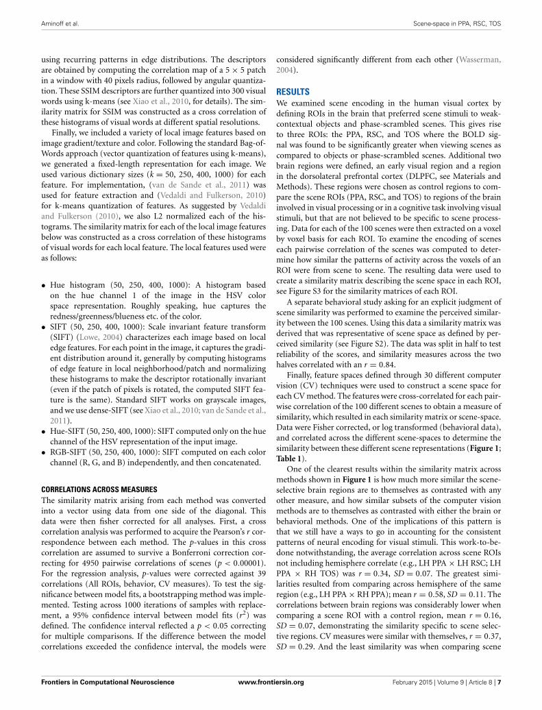
Finally, feature spaces defined through 30 different computervision (CV) techniques were used to construct a scene space foreach CV method. The features were cross-correlated for each pair-wise correlation of the 100 different scenes to obtain a measure ofsimilarity, which resulted in each similarity matrix or scene-space.Data were Fisher corrected, or log transformed (behavioral data),and correlated across the different scene-spaces to determine thesimilarity between these different scene representations (Figure 1;Table 1).

One of the clearest results within the similarity matrix acrossmethods shown in Figure 1 is how much more similar the scene-selective brain regions are to themselves as contrasted with anyother measure, and how similar subsets of the computer visionmethods are to themselves as contrasted with either the brain orbehavioral methods. One of the implications of this pattern isthat we still have a ways to go in accounting for the consistentpatterns of neural encoding for visual stimuli. This work-to-be-done notwithstanding, the average correlation across scene ROIsnot including hemisphere correlate (e.g., LH PPA × LH RSC; LHPPA × RH TOS) was r = 0.34, SD = 0.07. The greatest simi-larities resulted from comparing across hemisphere of the sameregion (e.g., LH PPA × RH PPA); mean r = 0.58, SD = 0.11. Thecorrelations between brain regions was considerably lower whencomparing a scene ROI with a control region, mean r = 0.16,SD = 0.07, demonstrating the similarity specific to scene selec-tive regions. CV measures were similar with themselves, r = 0.37,SD = 0.29. And the least similarity was when comparing scene

Frontiers in Computational Neuroscience www.frontiersin.org February 2015 | Volume 9 | Article 8 | 7

Aminoff et al. Scene-space in PPA, RSC, TOS

FIGURE 1 | Similarity matrix across different methods for constructing a

scene space. Each cell is the r -value computing the correlation between thesimilarity of one scene space (e.g., voxel space in LH PPA) with another (e.g.,attribute space in NEIL). Scene ROIs include the PPA, RSC, and TOS for each

hemisphere, and two control brain regions—an early visual region as well theDLPFC. Computer vision methods are grouped according to their nominallevel of representation—e.g., GEOM is mid-level (purple); and HOG islow-level (red).

brain ROIs with CV measures r = 0.04, SD = 0.06, however thecorrelations did get as high as r = 0.22, p < 1.5 × 1048 foundbetween the RH PPA and the SUN measures. Similarity matricesderived from low-level features such as SSIM and HOG wereeither non-significant or negatively correlated with voxel spacefrom scene regions, but found to be positively correlated with theearly visual ROI. In general, the high-level CV methods (NEIL,SUN) significantly correlated with the scene ROIs, where, the low-level CV methods showed little correlation (although some didreach significance, see Table 1). Suffice it to say, there is a greatdeal of room for improvement in using CV measures to explainbrain encoding of scenes. Critically, this is not due to noise in thesignal—as already mentioned, there are strong correlations acrossthe scene-selective ROIs, supporting the assumption that there isa meaningful code being used to process scenes, it just has yet tobe cracked. However, that we observe significant correlations withsome CV measures suggests we are making progress in explicat-ing this code, and that the continued search for correspondences

between computer vision models and patterns of brain activitymay prove fruitful.

A more surprising result from our study is that correlationswith brain regions was stronger with CV models (especially thosewith high- and mid- level features; average of SUN, NEIL, andGEOM All r = 0.11, SD = 0.05) than with behavioral similarityjudgments (average r = 0.05, SD = 0.01). From these results weinfer that perceived similarity between scenes is based on differentvisual and semantic parameters than those encoded in scene-selective ROIs. From an empirical point of view, the fact thatour neurally-derived scene spaces do correlate more with some ofthe scene spaces derived from CV models suggests that methodsdrawn from computer vision offer a tool for isolating specific, andperhaps more subtle, aspects of scene representation as encodedin different regions of the human brain.

Beyond examining the general correspondence between CVmetrics and the neural encoding of scenes, we were interested inthe nature of the CV metrics offering the best correspondence and

Frontiers in Computational Neuroscience www.frontiersin.org February 2015 | Volume 9 | Article 8 | 8

Aminoff et al. Scene-space in PPA, RSC, TOS

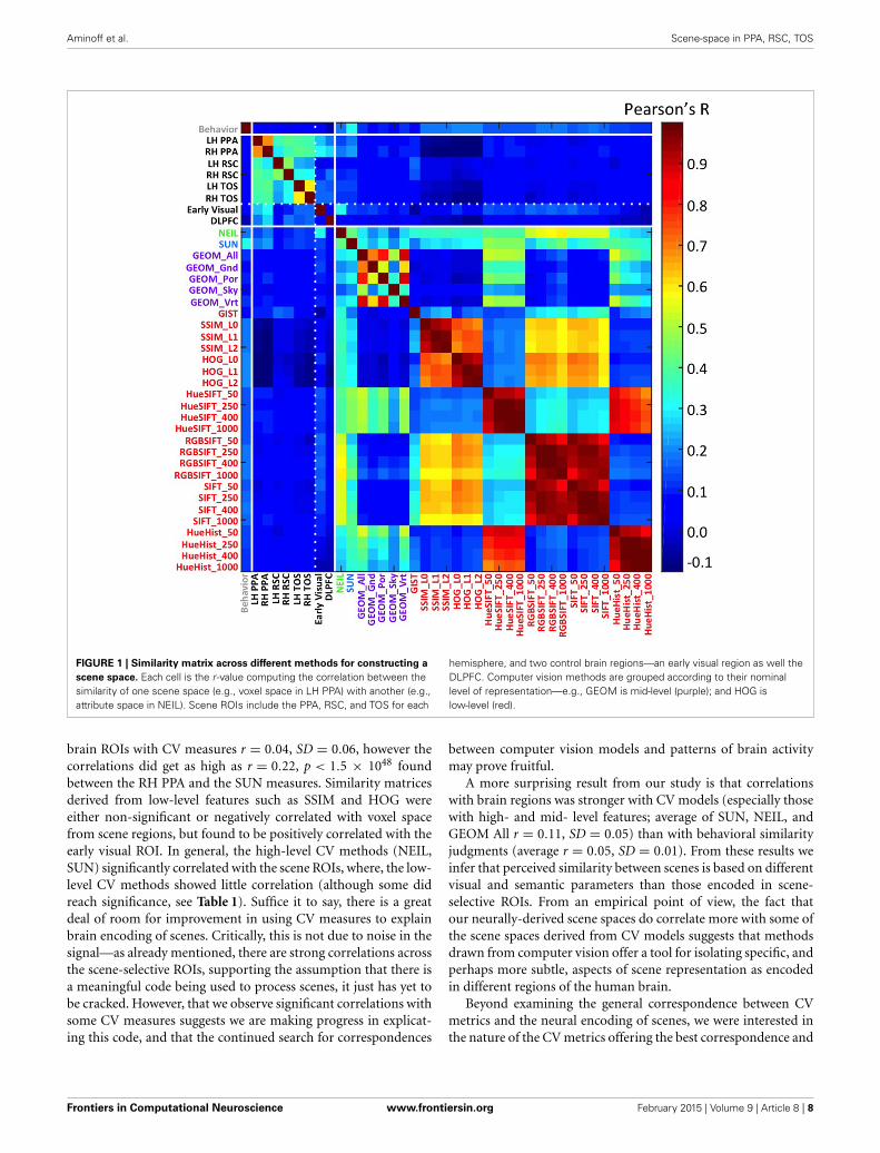
Table 1 | Pearson’s r-values for the correlations between similarity matrices.

Behavior LH+PPA RH+PPA LH+RSC RH+RSC LH+TOS RH+TOS Early+Visual DLPFC

Behavior 0.050 0.030 0.061 0.044 0.051 0.050 0.055 −0.044

NEIL 0.182 0.136 0.190 0.066 0.092 0.140 0.111 0.322 0.080

SUN 0.319 0.188 0.215 0.086 0.111 0.140 0.109 0.139 0.061

GEOM_All 0.107 0.067 0.085 0.055 0.070 0.089 0.077 0.111 0.042

GEOM_Gnd 0.078 0.038 0.048 0.045 0.059 0.053 0.054 0.133 0.015

GEOM_Por 0.094 0.079 0.115 0.043 0.067 0.058 0.060 0.100 0.054

GEOM_Sky 0.059 0.040 0.018 0.074 0.050 0.062 0.038 0.082 0.019

GEOM_Vrt 0.113 0.080 0.102 0.041 0.077 0.073 0.066 0.101 0.048

GIST 0.064 0.101 0.095 0.171 0.141 0.050 0.072 −0.057 0.032

SSIM_L0 0.182 −0.053 −0.071 0.005 0.006 −0.008 −0.028 0.088 −0.014

SSIM_L1 0.178 −0.070 −0.096 0.008 0.012 −0.019 −0.039 0.073 −0.024

SSIM_L2 0.175 −0.069 −0.093 0.011 0.018 −0.017 −0.036 0.087 −0.021

HOG_L0 0.201 −0.099 −0.131 −0.001 −0.015 −0.041 −0.074 0.108 −0.047

HOG_L1 0.193 −0.116 −0.151 0.014 0.000 −0.050 −0.075 0.085 −0.068

HOG_L2 0.198 −0.115 −0.157 0.025 0.005 −0.050 −0.072 0.072 −0.076

HueSIFT_50 0.151 0.105 0.105 0.013 0.038 0.083 0.066 0.154 0.025

HueSIFT_250 0.145 0.078 0.087 0.023 0.043 0.068 0.057 0.139 0.024

HueSIFT_400 0.151 0.096 0.100 0.028 0.045 0.076 0.064 0.128 0.021

HueSIFT_1000 0.153 0.087 0.090 0.035 0.049 0.066 0.057 0.116 0.014

RGBSIFT_50 0.156 0.007 0.029 0.011 0.033 0.009 −0.017 0.175 0.066

RGBSIFT_250 0.178 0.014 0.028 0.048 0.050 0.015 0.011 0.154 0.046

RGBSIFT_400 0.188 0.046 0.054 0.066 0.060 0.025 0.025 0.167 0.039

RGBSIFT_1000 0.188 0.077 0.087 0.083 0.076 0.046 0.052 0.153 0.048

SIFT_50 0.155 −0.002 0.025 0.018 0.043 0.006 −0.012 0.173 0.066

SIFT_250 0.173 0.018 0.037 0.045 0.048 0.010 0.005 0.136 0.058

SIFT_400 0.180 0.030 0.044 0.050 0.051 0.016 0.014 0.123 0.052

SIFT_1000 0.173 0.070 0.089 0.072 0.065 0.036 0.043 0.099 0.065

HueHist_50 0.137 0.061 0.055 0.001 0.029 0.068 0.045 0.093 0.003

HueHist_250 0.127 0.057 0.041 0.043 0.053 0.060 0.044 0.012 −0.017

HueHist_400 0.123 0.052 0.032 0.053 0.059 0.053 0.042 −0.012 −0.024

HueHist_1000 0.114 0.044 0.022 0.058 0.060 0.044 0.038 −0.033 −0.032

Gray values indicate p >0.05; and bolded values indicate survived correction for multiple correlations.

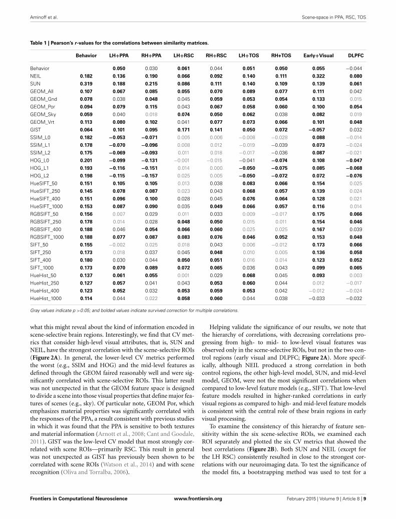
what this might reveal about the kind of information encoded inscene-selective brain regions. Interestingly, we find that CV met-rics that consider high-level visual attributes, that is, SUN andNEIL, have the strongest correlation with the scene-selective ROIs(Figure 2A). In general, the lower-level CV metrics performedthe worst (e.g., SSIM and HOG) and the mid-level features asdefined through the GEOM faired reasonably well and were sig-nificantly correlated with scene-selective ROIs. This latter resultwas not unexpected in that the GEOM feature space is designedto divide a scene into those visual properties that define major fea-tures of scenes (e.g., sky). Of particular note, GEOM Por, whichemphasizes material properties was significantly correlated withthe responses of the PPA, a result consistent with previous studiesin which it was found that the PPA is sensitive to both texturesand material information (Arnott et al., 2008; Cant and Goodale,2011). GIST was the low-level CV model that most strongly cor-related with scene ROIs—primarily RSC. This result in generalwas not unexpected as GIST has previously been shown to becorrelated with scene ROIs (Watson et al., 2014) and with scenerecognition (Oliva and Torralba, 2006).

Helping validate the significance of our results, we note thatthe hierarchy of correlations, with decreasing correlations pro-gressing from high- to mid- to low-level visual features wasobserved only in the scene-selective ROIs, but not in the two con-trol regions (early visual and DLPFC; Figure 2A). More specif-ically, although NEIL produced a strong correlation in bothcontrol regions, the other high-level model, SUN, and mid-levelmodel, GEOM, were not the most significant correlations whencompared to low-level feature models (e.g., SIFT). That low-levelfeature models resulted in higher-ranked correlations in earlyvisual regions as compared to high- and mid-level feature modelsis consistent with the central role of these brain regions in earlyvisual processing.

To examine the consistency of this hierarchy of feature sen-sitivity within the six scene-selective ROIs, we examined eachROI separately and plotted the six CV metrics that showed thebest correlations (Figure 2B). Both SUN and NEIL (except forthe LH RSC) consistently resulted in close to the strongest cor-relations with our neuroimaging data. To test the significance ofthe model fits, a bootstrapping method was used to test for a

Frontiers in Computational Neuroscience www.frontiersin.org February 2015 | Volume 9 | Article 8 | 9

Aminoff et al. Scene-space in PPA, RSC, TOS

FIGURE 2 | Strength of correlation between the similarity matrix of

computer vision (CV) metrics and the similarity matrix of patterns of

brain activity across voxels in each ROI. (A) The average correlation acrosseach CV metric and each of the scene ROIs is shown by the black bars. TheX-axis is ordered by the strength of this correlation. By way of comparison,the correlations between the CV metrics and the two control regions areillustrated by the light gray bars (early visual region) and the dark gray bars(DLPFC). Error bars indicate standard error across the six scene ROIs (LH and

RH of the PPA, RSC, TOS). Note that font color indicates the approximatelevel of featural analysis implemented in each specific CV metric: blue andgreen are high-level; purple is mid-level; and red is low-level. Numbersindicate the top 6 correlations in the early visual regions (light gray font,above light gray bars) and in the DLPFC (dark gray front, above dark graybars). (B) The top-ranked 6 CV metrics that correlated with theneurally-derived similarity matrix in each of the 6 scene-selective ROIs. TheY-axis is Pearson’s r -value.

Frontiers in Computational Neuroscience www.frontiersin.org February 2015 | Volume 9 | Article 8 | 10

Aminoff et al. Scene-space in PPA, RSC, TOS

p < 0.05 correcting for multiple correlations. For a full plot of allcorrelations, see Figure S4. Only in the LH PPA did the SUN fea-tures significantly account for more variance in brain data thanNEIL features, in the other ROIs they were statistically equiva-lent. The PPA and the TOS both had SUN and NEIL fitting thedata the best, performing significantly better than behavior, lowlevel features such as HueHist, SIFT, RGBSIFT. In some cases thevariances accounted for by HOG and SSIM, which was negativelycorrelated, did not significantly differ from SUN and NEIL (LHPPA, RH PPA, RH TOS). However, it is hard to interpret thesignificance of a negative correlation, so we provide this resultwith caution. Interestingly, color also seemed to be an impor-tant feature in encoding scene space. Hue SIFT, which takes intoaccount scale invariant local features with respect to differenthue maps, gave rise to scene spaces that were correlated with theneural responses measured in both TOS and demonstrated sig-nificance above a number of other models in the PPA. Althoughnumerically midlevel features—GEOM—correlated better thanlow level features, significance was only reached for GEOM_porand GEOM_sky in the RH PPA, and GEOM_all in the LHTOS. On the other hand, the RSC had a different pattern ofcorrelations. GIST showed the strongest correlation with our neu-roimaging data within the RSC, fitting significantly better than allother models in the LH RSC, and all models except for the SUNfeatures in the RH RSC. This is consistent with previous resultsdemonstrating a correspondence for GIST with the responsesof this region (Watson et al., 2014). In the LH RSC and RHRSC SUN features and RGB SIFT correlated at levels significantlyover other models, and within the RH RSC NEIL also correlatedsignificantly over and above other models. Overall, high-levelfeature models produced the scene spaces most consistently cor-related with the scene spaces derived from scene-selective ROIsin the PPA and TOS, whereas GIST correlated the best, andthe high-level SUN and NEIL features correlated next best inthe RSC.

To investigate the reliability of this dataset we split the datain two (one for each session) and tested the consistency of theresults. We found the correlations between the brain data withthe CV measures and behavioral judgments were very consistentover the two sessions, resulting in an average r = 0.76, SD = 0.19;where the strongest consistency was in the PPA and early visualregions r = 0.94, SD = 0.02, and the lowest consistency was inthe RH RSC (r = 0.43) and the DLPFC (r = 0.63). In addition,we examined the effect of including the trials that “jiggled” onthe analysis, until this point all analyses include the rotated trials.We performed the analyses with and without the rotated trials,showing very little effect of including all trials in the average, theaverage r-value obtained across all ROIs with the CV measuresand behavioral data across the two analyses was 0.97, SD = 0.02.The most notable difference in the analysis that did not includethe rotated trials was an increase in the correlation with GIST.This result provides some insight into the nature of the correla-tion between GIST and scene ROIs, one that may be less stablethan the others and therefore may not allow theoretical inferenceabout the nature of scene representations in these brain regions.

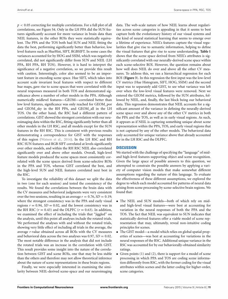
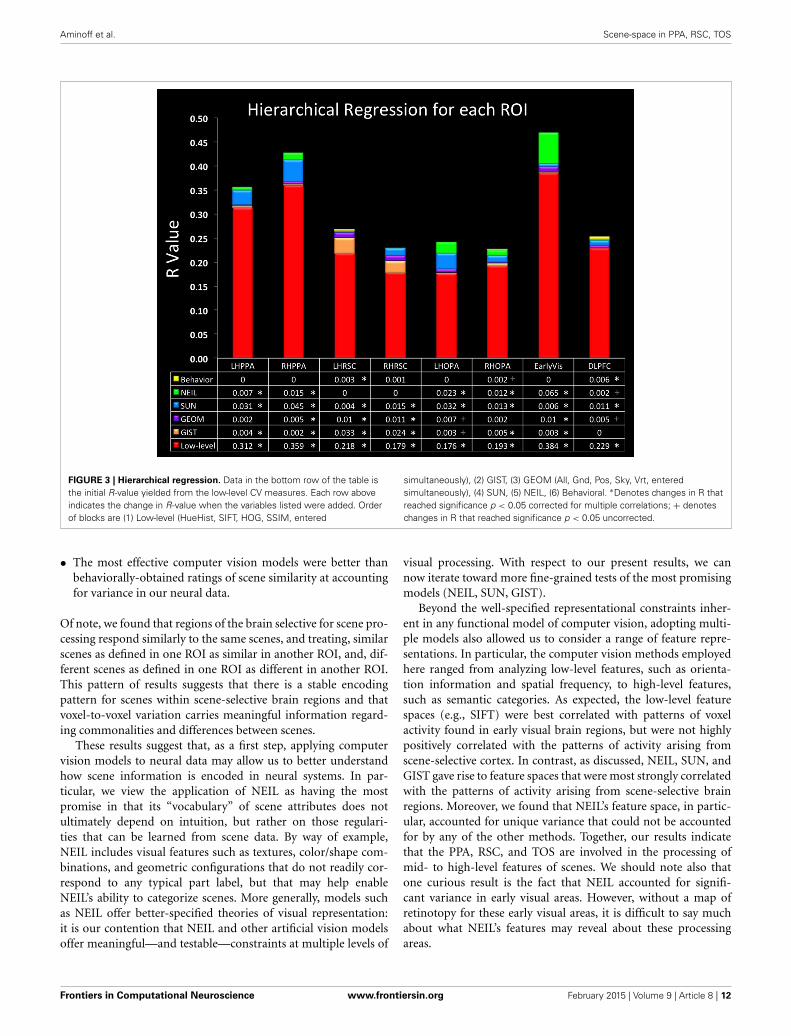
Finally, we were especially interested in examining the simi-larity between NEIL-derived scene-space and our neuroimaging

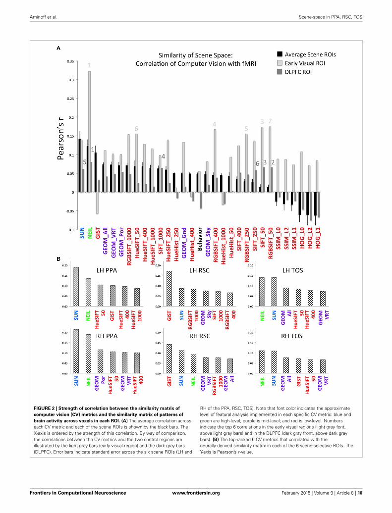
data. The web-scale nature of how NEIL learns about regulari-ties across scene categories is appealing in that it seems to bestcapture both the evolutionary history of our visual systems andthe kind of neural statistical learning that seems to emerge overa lifetime of experience. NEIL’s features capture the visual regu-larities that give rise to semantic information, helping to definethe visual features that give rise to scene understanding. Table 1shows that the scene space derived from NEIL’s attributes is sig-nificantly correlated with our neurally-derived scene space withineach scene-selective ROI. However, the question remains abouthow well does NEIL do over and above all the other CV mea-sures. To address this, we ran a hierarchical regression for eachROI (Figure 3). In this regression the first input was the low-levelCV metrics (Hue Histogram, SIFT, HOG, SSIM) and the secondinput was to separately add GIST, to see what variance was leftover when the low-level visual features were removed. Next weentered the GEOM metrics, followed by the SUN attributes, fol-lowed by NEIL, and, finally, the last block being our behavioraldata. This regression demonstrates that NEIL accounts for a sig-nificant amount of the variance in defining the neurally-derivedscene space over and above any of the other CV metrics in boththe PPA and the TOS, as well as in early visual regions. As such,it appears as if NEIL is capturing something unique about scenerepresentation within the PPA, TOS, and early visual regions thatis not captured by any of the other models. The behavioral dataonly accounted for unique variance above that already accountedfor in the LH RSC and the DLPFC.

DISCUSSIONWe started with the challenge of specifying the “language” of mid-and high-level features supporting object and scene recognition.Given the large space of possible answers to this question, weattempted to constrain the possible answers by applying a vari-ety of computer vision models that make somewhat differentassumptions regarding the nature of this language. To evaluatethe effectiveness of these different assumptions, we explored thedegree to which each model accounted for patterns of neural dataarising from scene processing by scene-selective brain regions. Wefound that:

• The NEIL and SUN models—both of which rely on mid-and high-level visual features—were best at accounting forvariation in the neural responses of both the PPA and theTOS. The fact that NEIL was equivalent to SUN indicates thatstatistically-derived features offer a viable model of scene rep-resentation that may, ultimately, reveal non-intuitive codingprinciples for scenes.

• The GIST model—a model which relies on global spatial prop-erties of scenes—was best at accounting for variations in theneural responses of the RSC. Additional unique variance in theRSC was accounted for by our behaviorally-obtained similarityratings.

• Given points (1) and (2), there is support for a model of sceneprocessing in which PPA and TOS are coding scene informa-tion differently from RSC, with the former coding for the visualattributes within scenes and the latter coding for higher-order,scene categories.

Frontiers in Computational Neuroscience www.frontiersin.org February 2015 | Volume 9 | Article 8 | 11

Aminoff et al. Scene-space in PPA, RSC, TOS

FIGURE 3 | Hierarchical regression. Data in the bottom row of the table isthe initial R-value yielded from the low-level CV measures. Each row aboveindicates the change in R-value when the variables listed were added. Orderof blocks are (1) Low-level (HueHist, SIFT, HOG, SSIM, entered

simultaneously), (2) GIST, (3) GEOM (All, Gnd, Pos, Sky, Vrt, enteredsimultaneously), (4) SUN, (5) NEIL, (6) Behavioral. ∗Denotes changes in R thatreached significance p < 0.05 corrected for multiple correlations; + denoteschanges in R that reached significance p < 0.05 uncorrected.

• The most effective computer vision models were better thanbehaviorally-obtained ratings of scene similarity at accountingfor variance in our neural data.

Of note, we found that regions of the brain selective for scene pro-cessing respond similarly to the same scenes, and treating, similarscenes as defined in one ROI as similar in another ROI, and, dif-ferent scenes as defined in one ROI as different in another ROI.This pattern of results suggests that there is a stable encodingpattern for scenes within scene-selective brain regions and thatvoxel-to-voxel variation carries meaningful information regard-ing commonalities and differences between scenes.

These results suggest that, as a first step, applying computervision models to neural data may allow us to better understandhow scene information is encoded in neural systems. In par-ticular, we view the application of NEIL as having the mostpromise in that its “vocabulary” of scene attributes does notultimately depend on intuition, but rather on those regulari-ties that can be learned from scene data. By way of example,NEIL includes visual features such as textures, color/shape com-binations, and geometric configurations that do not readily cor-respond to any typical part label, but that may help enableNEIL’s ability to categorize scenes. More generally, models suchas NEIL offer better-specified theories of visual representation:it is our contention that NEIL and other artificial vision modelsoffer meaningful—and testable—constraints at multiple levels of

visual processing. With respect to our present results, we cannow iterate toward more fine-grained tests of the most promisingmodels (NEIL, SUN, GIST).

Beyond the well-specified representational constraints inher-ent in any functional model of computer vision, adopting multi-ple models also allowed us to consider a range of feature repre-sentations. In particular, the computer vision methods employedhere ranged from analyzing low-level features, such as orienta-tion information and spatial frequency, to high-level features,such as semantic categories. As expected, the low-level featurespaces (e.g., SIFT) were best correlated with patterns of voxelactivity found in early visual brain regions, but were not highlypositively correlated with the patterns of activity arising fromscene-selective cortex. In contrast, as discussed, NEIL, SUN, andGIST gave rise to feature spaces that were most strongly correlatedwith the patterns of activity arising from scene-selective brainregions. Moreover, we found that NEIL’s feature space, in partic-ular, accounted for unique variance that could not be accountedfor by any of the other methods. Together, our results indicatethat the PPA, RSC, and TOS are involved in the processing ofmid- to high-level features of scenes. We should note also thatone curious result is the fact that NEIL accounted for signifi-cant variance in early visual areas. However, without a map ofretinotopy for these early visual areas, it is difficult to say muchabout what NEIL’s features may reveal about these processingareas.

Frontiers in Computational Neuroscience www.frontiersin.org February 2015 | Volume 9 | Article 8 | 12

Aminoff et al. Scene-space in PPA, RSC, TOS

Finally, we also observed that two models relying primarily onlow-level features were significantly correlated with certain scene-selective brain regions. First, GIST correlated quite strongly withthe RSC, replicating previous findings demonstrating a connec-tion between GIST and the RSC functional properties (Watsonet al., 2014). This suggests that the RSC may contribute to pro-cessing an image’s spatial envelope or global scene propertieswhich are known to be involved in scene understanding (Olivaand Torralba, 2006; Greene and Oliva, 2009). Moreover the RSChas been shown to process a representation of the scene that isabstracted from what is seen in the environment, typically pro-cessing a broader environment that extends beyond the currentsaccade (Epstein and Higgins, 2007; Park et al., 2007; Park andChun, 2009). One possibility is that the RSC may process thelow spatial frequencies or global properties of a scene that arestrongly indicative of scene category. In addition, RSC was foundto correlate with behavioral ratings of similarity, which was notfound in the PPA or the TOS. That the correlations with GIST andbehavior were unique to the RSC may suggest that RSC may pro-vide a more categorical, or high-order representation of scenes.The second low-level model proved to be important were SIFTfeatures in color domains that correlated strongly with multiplescene-selective regions: Hue SIFT showed strong correlations withthe PPA and TOS, while RGB SIFT showed strong correlationswith the RSC. In earlier work, junctures within scenes, whichmay be similar to SIFT features, were found to be importantfor scene categorization (Walther and Shen, 2014). Our resultsadd to this finding by suggesting that key features but specificallywithin different color domains also carry information regardingscene categories. That is, scene-selective brain regions may rely oncolor cues in scene understanding—a claim consistent with ear-lier behavioral research on scene processing (Oliva and Schyns,2000). At the same time, the lower correlations observed for theHue Histogram model as compared to the Hue SIFT and RGBSIFT models suggest that it is not color per se that carries thisinformation, but rather information about scene categories arisesfrom an interaction of SIFT features within color domains. In par-ticular, the perirhinal cortex—a region of the parahippocampalgyrus adjacent to the PPA—has been shown to unitize propertiesacross an object; for example, that stop signs are red (Staresinaand Davachi, 2010). As such, this function may extend to theparahippocampal region more generally being seen as unitizingdiagnostic features, with the PPA supporting this function withinscene processing.

In sum, we explored the visual dimensions underlying the neu-ral representation of scenes using an approach in which modelsderived from computer vision are used as proxies for any psycho-logical theory. While this approach may seem somewhat indirect,we argue that it is a necessary precursor in that extant psycho-logical models have typically been somewhat underspecified withrespect to the potential space of visual features. Humans canidentify scenes effortlessly under a wide variety of conditions.For example, we can name scenes with near-equivalent accuracywhen shown both photographs and line drawings, and with colorpresent or absent. There is, then, no single feature dimensionthat drives the organization of scene-selective cortex. However,some dimensions are likely to prove more effective than others.

Color is just one example of the many diagnostic cues that areused to aid in scene perception. There are almost surely a rangeof visual attributes and their associations within scenes that arediagnostic as to their categories and to which we are sensitive(Bar et al., 2008; Aminoff et al., 2013). Computer vision models,to the extent that they make representational assumptions withrespect to scene attributes and their associations (i.e., models witha less well-understood representational basis may not actually beparticularly informative), are, therefore, useful for better expli-cating those featural dimensions involved in human visual sceneprocessing.

ACKNOWLEDGMENTSSupported by Office of Naval Research—MURI contract numberN000141010934 and National Science Foundation 1439237. Wethank Carol Jew for help in data collection; and Ying Yang andTim Verstynen for technical assistance.

SUPPLEMENTARY MATERIALThe Supplementary Material for this article can be foundonline at: http://www.frontiersin.org/journal/10.3389/fncom.

2015.00008/abstract

REFERENCESAminoff, E. M., Kveraga, K., and Bar, M. (2013). The role of the parahip-

pocampal cortex in cognition. Trends Cogn. Sci. 17, 379–390. doi:10.1016/j.tics.2013.06.009

Arnott, S. R., Cant, J. S., Dutton, G. N., and Goodale, M. A. (2008). Crinklingand crumpling: an auditory fMRI study of material properties. Neuroimage 43,368–378. doi: 10.1016/j.neuroimage.2008.07.033

Baldassi, C., Alemi-Neissi, A., Pagan, M., DiCarlo, J. J., Zecchina, R., and Zoccolan,D. (2013). Shape similarity, better than semantic membership, accounts forthe structure of visual object representations in a population of monkeyinferotemporal neurons. PLoS Comput. Biol. 9:e1003167. doi: 10.1371/jour-nal.pcbi.1003167.s004

Bar, M., and Aminoff, E. (2003). Cortical analysis of visual context. Neuron 38,347–358. doi: 10.1016/S0896-6273(03)00167-3

Bar, M., Aminoff, E., and Schacter, D. L. (2008). Scenes unseen: the parahip-pocampal cortex intrinsically subserves contextual associations, not scenesor places per se. J. Neurosci. 28, 8539–8544. doi: 10.1523/JNEUROSCI.0987-08.2008

Barenholtz, E., and Tarr, M. J. (2007). “Reconsidering the role of structure invision,” in Categories in Use, Vol. 47, eds A. Markman and B. Ross (San Diego,CA: Academic Press), 157–180.

Cant, J. S., and Goodale, M. A. (2011). Scratching beneath the surface: new insightsinto the functional properties of the lateral occipital area and parahippocampalplace area. J. Neurosci. 31, 8248–8258. doi: 10.1523/JNEUROSCI.6113-10.2011

Cant, J. S., and Xu, Y. (2012). Object ensemble processing in humananterior-medial ventral visual cortex. J. Neurosci. 32, 7685–7700. doi:10.1523/JNEUROSCI.3325-11.2012

Chen, X., Shrivastava, A., and Gupta, A. (2013). “NEIL: extracting visual knowledgefrom web data,” in IEEE International Conference on Computer Vision (ICCV)(Sydney), 1409–1416.

Dalal, N., and Triggs, B. (2005). Histograms of oriented gradients for human detec-tion. IEEE Comput. Soc. Conf. Comput. Vis. Pattern Recogn. 1, 886–893. doi:10.1109/CVPR.2005.177

Diedrichsen, J., and Shadmehr, R. (2005). Detecting and adjusting forartifacts in fMRI time series data. Neuroimage 27, 624–634. doi:10.1016/j.neuroimage.2005.04.039

Epstein, R. A., and Higgins, J. S. (2007). Differential parahippocampal and retros-plenial involvement in three types of visual scene recognition. Cereb. Cortex 17,1680–1693. doi: 10.1093/cercor/bhl079

Farhadi, A., Endres, I., Hoiem, D., and Forsyth, D. (2009). “Describing objectsby their attributes,” in Proceedings of IEEE Conference on Computer Vision andPattern Recognition (CVPR) (Miami Beach, FL).

Frontiers in Computational Neuroscience www.frontiersin.org February 2015 | Volume 9 | Article 8 | 13

Aminoff et al. Scene-space in PPA, RSC, TOS

Felzenszwalb, P. F., Girshick, R. B., McAllester, D., and Ramanan, D. (2010). Objectdetection with discriminatively trained part-based models. Pattern Anal. Mach.Intell. IEEE Trans. 32, 1627–1645. doi: 10.1109/TPAMI.2009.167

Greene, M. R., and Oliva, A. (2009). Recognition of natural scenes from globalproperties: seeing the forest without representing the trees. Cogn. Psychol. 58,137–176. doi: 10.1016/j.cogpsych.2008.06.001

Harel, A., Kravitz, D. J., and Baker, C. I. (2013). Deconstructing visual scenes incortex: gradients of object and spatial layout information. Cereb. Cortex 23,947–957. doi: 10.1093/cercor/bhs091

Hoiem, D., Efros, A. A., and Hebert, M. (2007). Recovering surface layout from animage. Int. J. Comput. Vis. 75, 151–172. doi: 10.1007/s11263-006-0031-y

Khaligh-Razavi, S., and Kriegeskorte, N. (2014). Deep supervised, but not unsu-pervised, models may explain IT cortical representation. PLOS Comput. Biol.10:e1003915. doi: 10.1371/journal.pcbi.1003915

Kravitz, D. J., Peng, C. S., and Baker, C. I. (2011). Real-world scene representationsin high-level visual cortex: it’s the spaces more than the places. J. Neurosci. 31,7322–7333. doi: 10.1523/JNEUROSCI.4588-10.2011

Lampert, C., Nickisch, H., and Harmeling, S. (2013). Attribute-based classificationfor zero-shot visual object categorization. IEEE Trans. Pattern Anal. Mach. Intell.36, 453–465. doi: 10.1109/TPAMI.2013.140

Leeds, D. D., Seibert, D. A., Pyles, J. A., and Tarr, M. J. (2013). Comparing visualrepresentations across human fMRI and computational vision. J. Vis. 13, 25.doi: 10.1167/13.13.25

Lowe, D. G. (2004). Distinctive image features from scale-invariant keypoints. Int.J. Comput. Vis. 60, 91–110. doi: 10.1023/B:VISI.0000029664.99615.94

Naphade, M., Smith, J., Tesic, J., Chang, S., Hsu, W., Kennedy, L., et al. (2006).Large-scale concept ontology for multimedia. IEEE Multimedia Mag. 13, 86–91.doi: 10.1109/MMUL.2006.63

Nasr, S., Echavarria, C. E., and Tootell, R. B. H. (2014). Thinking outside thebox: rectilinear shapes selectively activate scene-selective cortex. J. Neurosci. 34,6721–6735. doi: 10.1523/JNEUROSCI.4802-13.2014

Nestor, A., Vettel, J. M., and Tarr, M. J. (2008). Task-specific codes for face recog-nition: how they shape the neural representation of features for detection andindividuation. PLoS ONE 3:e3978. doi: 10.1371/journal.pone.0003978

Oliva, A., and Schyns, P. G. (2000). Diagnostic colors mediate scene recognition.Cogn. Psychol. 41, 176–210. doi: 10.1006/cogp.1999.0728

Oliva, A., and Torralba, A. (2001). Modeling the shape of the scene: a holisticrepresentation of the spatial envelope. Int. J. Comput. Vis. 42, 145–175. doi:10.1023/A:1011139631724

Oliva, A., and Torralba, A. (2006). Building the gist of a scene: the role of globalimage features in recognition. Prog. Brain Res. 155, 23–36. doi: 10.1016/S0079-6123(06)55002-2

Park, S., Brady, T. F., Greene, M. R., and Oliva, A. (2011). Disentangling scenecontent from spatial boundary: complementary roles for the parahippocam-pal place area and lateral occipital complex in representing real-world scenes.J. Neurosci. 31, 1333–1340. doi: 10.1523/JNEUROSCI.3885-10.2011

Park, S., and Chun, M. M. (2009). Different roles of the parahippocampal placearea (PPA) and retrosplenial cortex (RSC) in panoramic scene perception.Neuroimage 47, 1747–1756. doi: 10.1016/j.neuroimage.2009.04.058

Park, S., Intraub, H., Yi, D.-J., Widders, D., and Chun, M. M. (2007). Beyond theedges of a view: boundary extension in human scene-selective visual cortex.Neuron 54, 335–342. doi: 10.1016/j.neuron.2007.04.006

Park, S., Konkle, T., and Oliva, A. (2014). Parametric coding of the size and clutterof natural scenes in the human brain. Cereb. Cortex. doi: 10.1093/cercor/bht418.[Epub ahead of print].

Patterson, G., and Hays, J. (2012). “Sun attribute database: discovering, annotating,and recognizing scene attributes,” in IEEE Conference on Computer Vision andPattern Recognition (CVPR) (Providence, RI), 2751–2758.

Shechtman, E., and Irani, M. (2007). “Matching local self-similarities across imagesand videos,” in IEEE Conference on Computer Vision and Pattern Recognition(CVPR) (Minneapolis, MN), 1–8.

Shrivastava, A., Singh, S., and Gupta, A. (2012). “Constrained semi-supervisedlearning using attributes and comparative attributes,” in Proceedings of EuropeanConference on Computer Vision (ECCV) (Florence), 369–383.

Stansbury, D. E., Naselaris, T., and Gallant, J. L. (2013). Natural scene statis-tics account for the representation of scene categories in human visual cortex.Neuron 79, 1025–1034. doi: 10.1016/j.neuron.2013.06.034

Staresina, B. P., and Davachi, L. (2010). Object unitization and associative memoryformation are supported by distinct brain regions. J. Neurosci. 30, 9890–9897.doi: 10.1523/JNEUROSCI.0826-10.2010

van de Sande, K. E., Gevers, T., and Snoek, C. G. (2011). Empoweringvisual categorization with the GPU. Multimedia IEEE Trans. 13, 60–70. doi:10.1109/TMM.2010.2091400

Vedaldi, A., and Fulkerson, B. (2010). VLFeat: an open and portable libraryof computer vision algorithms. Proc. Int. Conf. Multimedia 1469–1472. doi:10.1145/1873951.1874249

Vedaldi, A., Ling, H., and Soatto, S. (2010). Knowing a good feature when you see it:ground truth and methodology to evaluate local features for recognition. Stud.Comput. Intell. 285, 27–49. doi: 10.1007/978-3-642-12848-6_2

Walther, D. B., and Shen, D. (2014). Nonaccidental properties underlie humancategorization of complex natural scenes. Psychol. Sci. 25, 851–860. doi:10.1177/0956797613512662

Wasserman, L. (2004). “The bootstrap”, in All of Statistics: A Concise Courseof Statistical Inference (New York, NY: Springer Publishing Company),107–118.

Watson, D. M., Hartley, T., and Andrews, T. J. (2014). Patterns of response tovisual scenes are linked to the low-level properties of the image. Neuroimage99, 402–410. doi: 10.1016/j.neuroimage.2014.05.045

Xiao, J., Hays, J., Ehinger, K. A., Oliva, A., and Torralba, A. (2010). “Sundatabase: large-scale scene recognition from abbey to zoo,” in IEEE Conferenceon Computer Vision and Pattern Recognition (CVPR) (San Francisco, CA),3485–3492.

Yamins, D. L. K., Hong, H., Cadieu, C. F., Solomon, E. A., Seibert, D., andDiCarlo, J. J. (2014). Performance-optimized hierarchical models predict neuralresponses in higher visual cortex. Proc. Natl. Acad. Sci. U.S.A. 111, 8619–8624.doi: 10.1073/pnas.1403112111

Yu, F., Ji, R., Tsai, M., Ye, G., and Chang, S. (2012). “Weak attributes for large-scaleimage retrieval,” in IEEE Conference on Computer Vision and Pattern Recognition(CVPR) (Providence, RI), 2949–2956.

Conflict of Interest Statement: The authors declare that the research was con-ducted in the absence of any commercial or financial relationships that could beconstrued as a potential conflict of interest.

Received: 10 September 2014; accepted: 15 January 2015; published online: 04February 2015.Citation: Aminoff EM, Toneva M, Shrivastava A, Chen X, Misra I, Gupta A and TarrMJ (2015) Applying artificial vision models to human scene understanding. Front.Comput. Neurosci. 9:8. doi: 10.3389/fncom.2015.00008This article was submitted to the journal Frontiers in Computational Neuroscience.Copyright © 2015 Aminoff, Toneva, Shrivastava, Chen, Misra, Gupta and Tarr.This is an open-access article distributed under the terms of the Creative CommonsAttribution License (CC BY). The use, distribution or reproduction in other forums ispermitted, provided the original author(s) or licensor are credited and that the originalpublication in this journal is cited, in accordance with accepted academic practice. Nouse, distribution or reproduction is permitted which does not comply with these terms.

Frontiers in Computational Neuroscience www.frontiersin.org February 2015 | Volume 9 | Article 8 | 14