Embed Size (px)
Citation preview


Contents
Front Matter 1 1. Front End Paper 22. Preface 33. The Role of Statistics 84. Describing Data Sets 245. Measures of Central Tendency and Dispersion 446. Principles of Probability 807. Probability Distributions 1068. Sampling Distributions 1469. Estimating with Confidence Intervals 172
10. Hypothesis Testing 19811. Two Population Tests 23012. Analysis of Variance 27013. Simple Regression and Correlation 32014. Multiple Regression and Correlation 36815. Time Series and Index Numbers 40216. Chi-Square and Other Nonparametric Tests 45017. Quality Control Techniques 502
Back Matter 541 18. Appendix I: Business Report Writing 54319. Appendix II: Answers to Selected Even-Numbered Problems 54920. Appendix III: Statistical Tables 55921. Index 60622. Back End Paper 613
iii

Credits
Front Matter 1 1. Front End Paper: Chapter from Applied Statistics for Business and Economics: An Essentials Version, Third Edition by
Webster, 1998 22. Preface: Chapter from Applied Statistics for Business and Economics: An Essentials Version, Third Edition by Webster,
1998 33. The Role of Statistics: Chapter 1 from Applied Statistics for Business and Economics: An Essentials Version, Third
Edition by Webster, 1998 84. Describing Data Sets: Chapter 2 from Applied Statistics for Business and Economics: An Essentials Version, Third
Edition by Webster, 1998 245. Measures of Central Tendency and Dispersion: Chapter 3 from Applied Statistics for Business and Economics: An
Essentials Version, Third Edition by Webster, 1998 446. Principles of Probability: Chapter 4 from Applied Statistics for Business and Economics: An Essentials Version, Third
Edition by Webster, 1998 807. Probability Distributions: Chapter 5 from Applied Statistics for Business and Economics: An Essentials Version, Third
Edition by Webster, 1998 1068. Sampling Distributions: Chapter 6 from Applied Statistics for Business and Economics: An Essentials Version, Third
Edition by Webster, 1998 1469. Estimating with Confidence Intervals: Chapter 7 from Applied Statistics for Business and Economics: An Essentials
Version, Third Edition by Webster, 1998 17210. Hypothesis Testing: Chapter 8 from Applied Statistics for Business and Economics: An Essentials Version, Third Edition
by Webster, 1998 19811. Two Population Tests: Chapter 9 from Applied Statistics for Business and Economics: An Essentials Version, Third
Edition by Webster, 1998 23012. Analysis of Variance: Chapter 10 from Applied Statistics for Business and Economics: An Essentials Version, Third
Edition by Webster, 1998 27013. Simple Regression and Correlation: Chapter 11 from Applied Statistics for Business and Economics: An Essentials
Version, Third Edition by Webster, 1998 32014. Multiple Regression and Correlation: Chapter 12 from Applied Statistics for Business and Economics: An Essentials
Version, Third Edition by Webster, 1998 36815. Time Series and Index Numbers: Chapter 13 from Applied Statistics for Business and Economics: An Essentials
Version, Third Edition by Webster, 1998 40216. Chi-Square and Other Nonparametric Tests: Chapter 14 from Applied Statistics for Business and Economics: An
Essentials Version, Third Edition by Webster, 1998 45017. Quality Control Techniques: Chapter 15 from Applied Statistics for Business and Economics: An Essentials Version,
Third Edition by Webster, 1998 502
iv

Back Matter 541 18. Appendix I: Business Report Writing: Chapter from Applied Statistics for Business and Economics: An Essentials
Version, Third Edition by Webster, 1998 54319. Appendix II: Answers to Selected Even-Numbered Problems: Chapter from Applied Statistics for Business and
Economics: An Essentials Version, Third Edition by Webster, 1998 54920. Appendix III: Statistical Tables: Chapter from Applied Statistics for Business and Economics: An Essentials Version, Third
Edition by Webster, 1998 55921. Index: Chapter from Applied Statistics for Business and Economics: An Essentials Version, Third Edition by Webster,
1998 60622. Back End Paper: Chapter from Applied Statistics for Business and Economics: An Essentials Version, Third Edition by
Webster, 1998 613
v


Version, Third Edition
ep1
Statistical Analysis
Frequency distributions
Measures of central tendency
Measures of dispersion
Descriptive statistics
Sampling distributions
Confidence intervals
Addition formula
Multiplication formula
Principles of probability
Ungrouped data
Grouped data
Ungrouped data
Grouped data
Discrete data
Continuous data
Probability distributions
Normal distribution
Mean
Proportion
Mean and proportion
One population
Two populations
Hypotheses tests
Mean and proportion
One population
Two populations
Analysis of variance
Regression and correlation analysis
Simple regression
Multiple regression
Nonparametrics
Times series analysis
Index numbers
Quality control techniques
Inferential statistics

Version, Third Edition
ix
As with the earlier editions of this text, this third edition continues to stress the impor-tance of applying statistical analysis to the solution of common business problems. Everyopportunity is used to demonstrate the manner in which statistics can effectively facilitatethe many decisions that business managers face on an almost daily basis. Further, the pre-sentation has been condensed to present the material in a more concise and compliantform. Several pedagogical characteristics described below have also been added toenhance the instructional advantages presented in the text.
This third edition of Applied Statistics for Business and Economics: An EssentialsVersion can be used effectively in either a one-semester or two-semester statistics course.While the material has been compressed to permit a streamlined discussion typical of aone-semester course, topical coverage remains sufficient to challenge even those studentswho complete their initial exposure to statistical analysis in a two-semester sequence.
‘ Below is a brief description of pedagogical features contained in this edition.
Features Retained from Previous Edition
• Chapter BlueprintEach chapter opens with a flowchart showing the main topics to be covered and themanner in which they are interrelated. This allows the students the opportunity toorganize the process they can use to master the material in that chapter.
• Three-Part ExamplesEvery example of the statistical tools available to business decision-makers presents arealistic situation requiring a solution they typically face in managing a business.These examples consist of three parts. The first is the Problem Statement thatdescribes the dilemma that must be resolved. The second part provides a completeand coherent Solution to that problem. Perhaps most important to the students, andwhat is absent in many other statistics texts, is the Interpretation of that solution. Itdoes no good for students to solve a problem if they do not understand what that solu-tion means.
• A Procedure for Business Report WritingCommunication in business is inarguably essential. In order for a business to functionas a unit, the individuals within that business must be able to communicate their ideasand thoughts. Appendix I describes and illustrates the manner in which a businessreport must be prepared in order to communicate essential proposals and recommen-dations to others who are interested in the results. Without this important skill, deci-sion-makers are grossly disadvantaged in their efforts to manage a business.
• Solved Problems Each chapter also concludes with problems and elaborate solutions that reinforce thestatistical tools presented in that chapter. This feature provides a convenient and help-ful summary of the crucial tools students are expected to master.
Preface

Version, Third Edition
x Preface
• List of Formulas A handy list of all formulas presented in the chapter and a brief description of theiruse is also provided at the close of all chapters.
• Computer ApplicationsInstructions are provided to show how the statistical tools can be performed on thecomputer. Computer printouts with emphasis on Minitab and Excel are presentedalong with a discussion of their important features.
• Computer ExercisesThe text comes with data disk containing several data files that can be accessed inMinitab, Excel, and ASCII formats. Each chapter provides the students with a prob-lem they must solve based on the data in one of those files with the aid of the statisti-cal tools discussed in that chapter. This provides the students with a realistic situationrequiring the applications of the statistical techniques to the computer-based data set.
• Chapter ProblemsAt the end of each chapter there is an ample supply of problems with a varying degreeof difficulty that allow the students the opportunity to sharpen and refine their statisti-cal skills. Again, these problems are of an applied nature that clearly demonstratehow statistics can aid in the business decision-making process.
New Features Added in the Third Edition
• Section ExercisesFollowing each section within each chapter are several exercises the students mustsolve that reinforce their understanding of the material to which they have beenexposed. This provides immediate feedback as to whether the students sufficientlycomprehend the material in that section before proceeding on to the next.
• Setting the StageEach chapter opens with a short narrative called Setting the Stage that presents a real-istic case that can best be addressed using the statistical tools contained in the chapter.The nature of the problem that must be resolved is described and thus provides thestudents with a foundation upon which to base their readings and examination of thechapter material.
• Curtain CallA short section at the close of each chapter entitled Curtain Call refers the studentsback to Setting the Stage. Additional data and information are provided instructingthe students to resolve the situation proposed in Setting the Stage by using the knowl-

Version, Third Edition
Preface xi
edge they have acquired in the chapter. This exercise combines the entire chapter intoa single “package” that enhances students’ overall comprehension of the material andeffectively ties up all loose ends.
• From Stage to Real LifeThe final segment in each chapter provides Web sites on the Internet that students canaccess to find additional data and information that can be used for further statisticalstudy. These Web sites are specially selected to relate to the issues and concernsraised in Setting the Stage and Curtain Call.
AcknowledgmentsWriting a text is a major undertaking that could not be accomplished without the help ofmany others. I would be remiss if I did not thank the many reviewers who examined oneor more of the several drafts of the manuscript for this text. These reviewers made sub-stantial contributions to the form and substance of the finished product:
Robert TrombleyDeVry Institute of Technology, Phoenix
Ziayien HwangUniversity of Oklahoma
Sandra StrasserValparaiso University
Barbara McKinneyWestern Michigan University
Diane StehmanNortheastern Illinois University
Nicholas FarnumCalifornia State University, Fullerton
W. Robert ReedUniversity of Oklahoma
Emmanuel EgbeMedgar Evers College
Sharad ChitgopekarIllinois State University
Robert HannumUniversity of Denver
Wendy McGuireSanta Fe Community College
Frank ForstLoyola University
Benny LoNorthwestern Polytechnic University

Version, Third Edition
With the large number of examples, exercises, and other numerical computations, itwould be impossible for any one person to correctly calculate and record every oneof them. Wendy McGuire and Mitchell Spiegel accuracy checked the computations inthe text.
Writing the supplements is a task unto itself and these authors deserve a round ofapplause: Wendy McGuire wrote the Student Study Guide that will be valuable to everystudent taking this course. Kilman Shin authored the computer guides for SPASS, SAS,and Minitab. With his in-depth knowledge of many software packages and of applied sta-tistics, he was able to write these guides, which will be of great benefit to anyone using orlearning to use, any of these three statistical packages. Ronald Merchant, Renee Goffinet,and Virginia Koehler prepared Applied Statistics for Business and Economics UsingExcel. This workbook empowers students to use Excel to solve many statistical problemsand was prepared using examples and problems from the text.
.Allen L. Webster
xii Preface


Version, Third Edition
0002
C H A P T E R1The Role of Statistics

Version, Third Edition
3
Role of Statistics
Importance ofand need forstatistics
DefinitionsImportance ofsampling
Functions ofstatistics
Careeropportunities
Levels ofmeasurements
Populationsand parameters
Samples andstatistics
Variables
Continuous
Discrete
Descriptivestatistics
Inferentialstatistics
Nominal
Ordinal
Interval
RatioSamplingerror
Chapter BlueprintThis chapter introduces the concept of statistics as an organized study. You will be exposed to the gen-eral purpose of statistical analysis and the many ways in which statistics can help you find solutionsto problems in your professional life.

Version, Third Edition
4 The Role of Statistics
S E T T I N G T H E S T A G EFortune (December 9,1996) reports that a hiringfrenzy has created a “sell-
ers’ labor market for nerds.” The race fortalent in the info-technology sector has gen-erated such intense competition for “quantjocks and computer nerds” that job seekerswith even minimum quantitative skills arebesieged with offers. Talent is so scarce anddemand is so high that companies are hiringable high schoolers and other companies aretrying to steal them away.
Pete Davis, a senior systems and net-working engineer for TIAC, an Internet ser-vice provider in Bedford, Massachusetts,has received at least 15 job offers since tak-ing his present position—which isn’t badfor someone who’s all of 18 years old. Re-cruiters call or E-mail Davis with attractivestock options and lucrative pay raises. Al-though Davis’ position is not entirely typi-cal, the battle is on for employees who aretrained in data analysis.
The strategy seems to paying off forbusinesses that aggressively seek out youngtalent capable of analyzing and understand-
ing quantitative information. As the charthere shows, the profits of these firms haveresponded favorably, rising much fasterthan the profits of companies that are drag-ging their heels when it comes to enteringthe information age. The Education IndustryReport, of St. Cloud, Minnesota, preparedan index of the profits of 15 firms that ag-gressively seek employees who can managedata and apply basic statistical and analyti-cal thought to common business problems.This index, the Data Management AlertAssessment (DMAA) was compared to theNational Association of Security DealersAutomated Quotations (NASDAQ) index.The results are obvious. The returns to firmshiring people who possess fundamentalknowledge of statistics far outstrip thoseof firms that have not yet seen the light.The recognition by a growing number ofbusinesses that effective managers need atleast a rudimentary knowledge of statisticalthought has precipitated, in the words ofFortune, a race for talent that resembles theagrarian frenzy of the Great Oklahoma LandGrab.
40
35
30
25
20
15
10
5
01993 1994 1995 1996
DMAA NASDAQ
Percentage Increase in Profits

Version, Third Edition
Chapter One 5
1.1 IntroductionAs our world grows in complexity, it becomes increasingly difficult to make informed andintelligent decisions. Often these decisions must be made with less than perfect knowledgeand in the presence of considerable uncertainty. Yet solutions to these problems are essen-tial to our well-being and even our ultimate survival. We are continually pressured by dis-tressing economic problems such as raging inflation, a cumbersome tax system, and exces-sive swings in the business cycle. Our entire social and economic fabric is threatened byenvironmental pollution, a burdensome public debt, an ever-increasing crime rate, and un-predictable interest rates.
If these conditions seem characteristic of today’s lifestyle, you should be remindedthat problems of this nature contributed more to the downfall of ancient Rome than did theinvasion of barbarian hordes from the North. Our relatively short period of success on thisplanet is no guarantee of future survival. Unless viable solutions to these pressing problemscan be found, we may, like the ancient Romans, follow the dinosaur and the dodo bird intooblivion.
This chapter will provide a general impression of what statistics is and how it can beuseful to you. This overview of the nature of statistics and the benefits it can contribute willbe accomplished by examining:
● Basic definitions of statistical tools.
● How sampling can be used to perform statistical analyses.
● The functions that statistics performs.
● How statistics can help you in your career.
We begin with a brief discussion of the meaningful role statistics plays in the importantprocess of making delicate decisions.
1.2 The Importance of StatisticsVirtually every area of serious scientific inquiry can benefit from statistical analysis. Forthe economic policymaker who must advise the president and other public officials onproper economic procedure, statistics has proved to be an invaluable tool. Decisionsregarding tax rates, social programs, defense spending, and many other issues can bemade intelligently only with the aid of statistical analysis. Businessmen and business-women, in their eternal quest for profit, find statistics essential in the decision-makingprocess. Efforts at quality control, cost minimization, product and inventory mix, and ahost of other business matters can be effectively managed by using proven statisticalprocedures.
For those in marketing research, statistics is of invaluable assistance in determiningwhether a new product is likely to prove successful. Statistics is also quite useful in theevaluation of investment opportunities by financial consultants. Accountants, personnelmanagers, and manufacturers all find unlimited opportunities to utilize statistical analysis.Even the medical researcher, concerned about the effectiveness of a new drug, finds statis-tics a helpful ally.
Such applications and many others are repeatedly illustrated in this text. You will beshown how to use statistics to improve your job performance and many aspects of yourdaily life.

Version, Third Edition
6 The Role of Statistics
1.3 Career Opportunities in StatisticsIn a few short years, you will leave the relative safety of your academic environment andbe thrust headlong into the competitive world of corporate America. From a practicalstandpoint, you may be interested in how you can use your statistical background aftergraduation. There is no doubt that an academic experience heavily laced with a strongquantitative foundation will greatly enhance your chances of finding meaningful employ-ment and, subsequently, demonstrating job competence.
When you find that dream job on the fast track of professional success, your employerwill expect you to do two things:
1. Make decisions.
2. Solve problems.
These duties can be accomplished through the application of statistical procedures.
A. The Universal Application of StatisticsBy becoming able to solve problems and make decisions, you will place yourself in highdemand in the job market. If you can make incisive decisions while solving someone’sproblems, he or she will certainly be willing to reward you handsomely. The world oftenpays more to people who can ask the right questions to achieve fundamental objectivesthan to those charged with the responsibility of carrying them out. The answers are oftenquite obvious once the right questions have been asked. Statistical analysis will prove to bea great benefit in the proper formulation of these essential questions.
Employers recognize that the complex problems faced in today’s world require quan-titative solutions. An inability to apply statistics and other quantitative methods to the manycommon problems you encounter will place you at a stark disadvantage in the job market.
Almost all areas of study require statistical thought. Courses of study that dependheavily upon statistical analysis include, but are not limited to, marketing, finance, eco-nomics, and operations research. The principles learned in accounting and managementalso rely on statistical preparation.
Financial and economic analysts must often rely on their quantitative skills to deviseeffective solutions for difficult problems. An understanding of economic and financialprinciples permits you to apply statistical techniques to reach viable solutions and makedecisions. Those of you aspiring to management or accounting positions, to be self-employed, or to obtain other careers in the industrial sector will find that a basic under-standing of statistics not only improves your chances of obtaining a position but alsoenhances the likelihood of promotion by enriching your job performance.
Those persons employed in quantitative areas working with statistical proceduresoften enjoy higher salaries and avoid the dreadful dead-end jobs. Furthermore, early intheir careers they usually find themselves in closer contact with high-level management.The proximity to the executive elite occurs because upper management needs the informa-tion and assistance which statistically trained people can provide. In the current labor mar-ket, employers simply do not want to hire or retain the statistically illiterate.
Whether your career aspirations tend toward private industry, public service with thegovernment, or some other source of gainful livelihood, you will be much better served byyour academic experience if you acquire a solid background in the fundamentals of statis-tical analysis.

Version, Third Edition
Chapter One 7
B. Total Quality ManagementAs world competition intensifies, there arises an increased effort on the part of businessesto promote product quality. This effort, broadly referred to as total quality management(TQM), has as its central purpose the promotion of those product qualities considered im-portant by the consumer. These attributes range from the absence of defects to rapid serviceand swift response to customer complaints. Today, most large businesses (as well as manysmaller ones) have quality control (QC) departments whose function it is to gather perfor-mance data and resolve quality problems. Thus, TQM represents a growing area of oppor-tunity to those with a statistical background.
TQM involves the use of integrated management teams consisting of engineers, mar-keting experts, design specialists, statisticians, and other professionals who can contributeto consumer satisfaction. The formulation of these teams, termed quality function deploy-ment (QFD), is designed to recognize and promote customer concerns. Working jointly, thespecialists interact to encourage product quality and effectively meet consumer needs andpreferences.
Another common method of promoting product quality is the use of quality controlcircles. QC circles consist of a small group of employees (usually between 5 and 12) whomeet regularly to solve work-related problems. Often consisting of both line workers andrepresentatives of management, the members of these QC circles are all from the samework area, and all receive formal training in statistical quality control and group planning.Through open discussion and statistical analysis, QC circles can achieve significant im-provement in various areas ranging from quality improvement, product design, productiv-ity, and production methods, to cost reduction and safety. It is estimated that over 90 per-cent of Fortune 500 companies effectively use QC circles.
One of the most important elements of TQM is a body of statistical tools and meth-ods used to promote statistical quality control (SQC). These tools help to organize andanalyze data for the purpose of problem solving. One of these tools is the Pareto chart.Named after the Italian economist Vilfredo Pareto, this diagram identifies the qualityproblems that occur most often or that prove to be the most costly. Figure 1.1 shows aPareto chart of the defects affecting the production of microwave ovens marketed byJC Penney.
Pareto charts often express the 80�20 rule: 80 percent of all problems are due to 20 per-cent of the causes. As Figure 1.1 shows, approximately 75 percent of all the problems arecaused by the auto defrost feature and the temperature hold feature of the oven.
Figure 1.1Pareto Chart
Perc
enta
ge o
f de
fect
s
50
40
30
0Auto
defrostfeature
Temperaturehold feature
Autostart
Touchpads
Stagecooking
Defect
20
10
Source: QC Circle, JC Penney, 1993.

Version, Third Edition
8 The Role of Statistics
Broadly speaking, SQC is designed to assure that products meet minimum productionstandards and specifications. This objective is often furthered through the use of accep-tance sampling, which is an integral part of SQC. Acceptance sampling involves testing arandom sample of existing goods to determine whether the entire shipment, or lot, shouldbe accepted. This decision is based in part on an acceptable quality level (AQL), which isthe maximum number or rate of defects that a firm is willing to tolerate.
There is a growing realization among businesses that product quality must be main-tained. If a firm is to compete successfully, it must take every precaution to ensure that itsproducts meet certain basic standards. The importance of TQM can therefore not beoveremphasized. The principles inherent in TQM are growing in popularity; they representthe future direction of applied statistical analysis in the business world. We will examineTQM in depth in Chapter 15.
C. You Will Have a Need for Statistical LiteracyYou may believe that the type of work you intend to pursue will not require statisticalanalysis. Or you may argue that the staff of statisticians employed by your company willperform the necessary statistical work, and there is no need for you to master the details ofstatistical analysis.
Such is not the case. Even if the professional statisticians in your organization performthe necessary statistical work for you, it is still essential that you possess a certain level ofstatistical literacy. To determine how the statistical staff can assist you in your job perfor-mance, you must know what statistics is, what statisticians do, and how they go aboutdoing it. When problems arise you must be able to determine how statistics can be of help.To do so, you must understand statistical procedures and be able to communicate with sta-tisticians in a joint effort to design adequate solutions and render optimal decisions. Onceyou have acquired this solid familiarity with statistical analysis, you will marvel at the lim-itless ways statistics can assist you in solving problems that often arise in a business setting.
1.4 Some Basic DefinitionsEvery branch of scientific inquiry has its unique vocabulary. Statistics is no exception. Thissection examines some common terms used in statistical analysis. These definitions andexpressions are essential to any comprehension of how statistical tests are carried out.
A. Populations and ParametersIn any statistical study, the researcher is interested in a certain collection or set of observa-tions called the population (or universe). If the incomes of all 121 million wage earners inthe United States are of interest to an economist assisting Congress in formulating a nationaltax plan, then all 121 million incomes constitute the population. If a tax plan is being consid-ered only for those incomes in excess of, say, $100,000, then those incomes above $100,000are the population. The population is the entire collection of all observations of interest.
Population A population is the entire collection of all observations of interest to theresearcher.

Version, Third Edition
Chapter One 9
If the chief executive officer (CEO) for a large manufacturing firm wishes to study the out-put of all the plants owned by the firm, then the output of all plants is the population.
A parameter is any descriptive measure of a population. Examples are the average in-come of all those wage earners in the United States, or the total output of all the manufac-turing plants. The point to remember is that a parameter describes a population.
Parameter A parameter is a descriptive measure of the entire population of all ob-servations of interest to the researcher.
B. Samples and StatisticsAlthough statisticians are generally interested in some aspect of the entire population, theygenerally find that populations are too big to study in their entirety. Calculating the averageincome of all the 121 million wage earners would be an overwhelming task. Therefore, wemust usually be content to study only a small portion of that population. This smaller andmore manageable portion is called a sample. A sample is a scientifically selected subset ofthe population.
Sample A sample is a representative portion of the population which is selected forstudy because the population is too large to examine in its entirety.
Each month the U.S. Department of Labor calculates the average income of a sampleof only several thousand wage earners selected from the entire population of all 121 mil-lion workers. The average from this sample is then used as an estimate of the average in-come for the entire population. Samples are necessary because studying entire populationsis too time-consuming and costly.
A statistic is any descriptive measure of a sample. The average income of those sev-eral thousand workers computed by the Department of Labor is a statistic. The statistic isto the sample what the parameter is to the population. Of importance, the statistic serves asan estimate of the parameter. Although we are really interested in the value of the parame-ter of the population, we most often must be resigned to only estimating it with a statisticfrom the sample we have selected.
Statistic A statistic describes a sample and serves as an estimate of the corre-sponding population parameter.
C. VariablesA variable is the characteristic of the sample or the population being observed. If the sta-tistical advisor for the mayor of San Francisco is interested in the distance commuters mustdrive each morning, the variable is miles driven. In a study concerning the income of wageearners in the United States, the variable is income.

Version, Third Edition
10 The Role of Statistics
Variable A variable is the characteristic of the population that is being examined inthe statistical study.
A variable can be (1) quantitative or (2) qualitative. If the observations can be ex-pressed numerically, it is a quantitative variable. The incomes of all the wage earners is anexample of a quantitative population. Other examples include the heights of all people wemight be interested in, scores students receive on a final examination in statistics, and thenumber of miles those commuters in San Francisco must drive each morning. In each case,the observations are measured numerically.
A qualitative variable is measured nonnumerically. The marital status of credit appli-cants, the sex of students in your statistics class, and the race, hair color, and religious pref-erence of those San Francisco commuters are examples of qualitative variables. In everycase, the observations are measured nonnumerically.
In addition, variables can be (1) continuous or (2) discrete. A continuous variable isone that can take on any value within a given range. No matter how close two observationsmay be, if the instrument of measurement is precise enough, a third observation can befound which will fall between the first two. A continuous variable generally results frommeasurement.
A discrete variable is restricted to certain values, usually whole numbers. They areoften the result of enumeration or counting. The number of students in your class and thenumber of cars sold by General Motors are examples. In neither case will you observe frac-tional values.
Throughout your study of statistics you will repeatedly refer to these concepts andterms. You must be aware of the role each plays in the process of statistical analysis. It isparticularly important that you be able to distinguish between a population and its parame-ters, and a sample and its statistics.
1.5 The Importance of SamplingAs noted, much of a statistician’s work is done with samples. Samples are necessary becausepopulations are often too big to study in their entirety. It is too time-consuming and costly toexamine the entire population, and we must select a sample from the population, calculatethe sample statistic, and use it to estimate the corresponding population parameter.
This discussion of samples leads to a distinction between the two main branches of sta-tistical analysis: (1) descriptive statistics and (2) inferential statistics. Descriptive statis-tics is the process of collecting, organizing, and presenting data in some manner thatquickly and easily describes these data. Chapters 2 and 3 examine descriptive statistics andillustrate the various methods and tools that can be used to present and summarize largedata sets.
Inferential statistics involves the use of a sample to draw some inference, or con-clusion, about the population from which that sample was taken. When the Departmentof Labor uses the average income of a sample of several thousand workers to estimatethe average income of all 121 million workers, it is using a simple form of inferentialstatistics.
The accuracy of any estimate is of extreme importance. This accuracy depends in largepart on the manner in which your sample was taken, and how careful you are to ensure that

Version, Third Edition
Chapter One 11
the sample provides a reliable image of the population. However, all too often, the sampleproves not to be fully representative of the population, and sampling error will result.Sampling error is the difference between the sample statistic used to estimate the popula-tion parameter and the actual but unknown value of the parameter.
Sampling Error Sampling error is the difference between the unknown populationparameter and the sample statistic used to estimate the parameter.
There are at least two possible causes of sampling error. The first source of samplingerror is mere chance in the sampling process. Due to the luck of the draw in selecting thesample elements, it is possible to unknowingly choose atypical elements that misrepresentthe population. In the effort to estimate the population mean, for example, it is possible toselect elements in the sample that are abnormally large, thereby resulting in an overesti-mation of the population mean. On the other hand, the luck of the draw may produce a largenumber of sample elements that are unusually small, causing an underestimation of the pa-rameter. In either case, sampling error has occurred.
A more serious form of sampling error is sampling bias. Sampling bias occurs whenthere is some tendency in the sampling process to select certain sample elements over oth-ers. If the sampling procedure is incorrectly designed and tends to promote the selection oftoo many units with a particular characteristic at the expense of units without that charac-teristic, the sample is said to be biased. For example, the sampling process may inherentlyfavor the selection of males to the exclusion of females, or married persons to the exclusionof singles.
Sampling Bias Sampling bias is the tendency to favor the selection of certain sam-ple elements over others.
A more thorough treatment of sampling bias is presented in a later chapter. Although sam-pling error can never be measured, since the parameter remains unknown, we must beaware that it is likely to occur.
1.6 The Functions of StatisticsWe have repeatedly emphasized the usefulness of statistics and the wide variety of prob-lems that it can solve. In order to more fully illustrate this wide applicability, let us exam-ine the various functions of statistics. Statistics is the science concerned with the (1) col-lection, (2) organization, (3) presentation, (4) analysis, and (5) interpretation of data.
Although the first step in any statistical study is the collection of the data, it is commonpractice in a beginning statistics course to assume that the data have already been collectedfor us and now lie at our disposal. Therefore, our work begins with the effort to organizeand present these data in some meaningful and descriptive manner. The data must be putinto some logical order that tends to quickly and readily reveal the message they contain.This procedure constitutes the process of descriptive statistics, as defined, and is discussedin the next few chapters. After the data have been organized and presented for examination,the statistician must analyze and interpret them. These procedures rely on inferential

Version, Third Edition
12 The Role of Statistics
Table 1.1Nominal Measuresof Investment Funds
Category/Fund Name
Aggressive Growth Money Market FundsTwenty Century Growth Alger PortfolioJanus Mariner Government
Total Return Tax-ExemptScudder Kemper MunicipalsVanguard StarPaxWorldUSAA Cornerstone
BondsStrong Short-TermScudder Short-Term
Source: Money, July 1992.
statistics and constitute a major benefit of statistical analysis by aiding in the decision-making and problem-solving process.
You will find that through the application of precise statistical procedures, it is pos-sible to actually predict the future with some degree of accuracy. Any business firm facedwith competitive pressures can benefit considerably from the ability to anticipate businessconditions before they occur. If a firm knows what its sales are going to be at some timein the near future, management can devise more accurate and more effective plans re-garding current operations. If future sales are estimated with a reliable degree of accu-racy, management can easily make important decisions regarding inventory levels, rawmaterial orders, employment requirements, and virtually every other aspect of businessoperations.
1.7 Levels of MeasurementVariables can be classified on the basis of their level of measurement. The way we classifyvariables greatly affects how we can use them in our analysis. Variables can be (1) nomi-nal, (2) ordinal, (3) interval, or (4) ratio.
A nominal measurement is created when names are used to establish categories intowhich variables can be exclusively recorded. For example, sex can be classified as “male”or “female.” You could also code it with a “1” or a “2,” but the numbers would serve onlyto indicate the categories and would carry no numerical significance; mathematical calcu-lations using these codes would be meaningless. Soft drinks may be classified as Coke,Pepsi, 7-Up, or Ale 8. Each drink could be recorded in one of these categories to the ex-clusion of the others.
Nominal Measurements Names or classifications are used to divide data into sepa-rate and distinct categories.
Table 1.1 illustrates the manner in which Money magazine classified different invest-ment funds. Notice that each fund is placed in a particular category based on its financialbehavior.

Version, Third Edition
Chapter One 13
Table 1.2An Ordinal Rankingof Investment Risk
Investment Risk Factor
Gold Very highSmall-growth companies Very highMaximum capital gains HighInternational HighOption income LowBalanced Low
It is important to remember that a nominal measurement carries no indication of orderof preference, but merely establishes a categorical arrangement into which each observa-tion can be placed.
Unlike a nominal measurement, an ordinal scale produces a distinct ordering orarrangement of the data. That is, the observations are ranked on the basis of some criterion.Sears Roebuck, one of the nation’s largest retailers, ranks many of its products as “good,”“better,” and “best.” Opinion polls often use an ordinal scale such as “strongly agree,”“agree,” “no opinion,” “disagree,” and “strongly disagree.”
As with nominal data, numbers can be used to order the rankings. Like nominal data,the magnitude of the numbers is not important; the ranking depends only on the order ofthe values. Sears could have used the rankings of “1,” “2,” and “3,” or “1,” “3,” and “12,”for that matter. The arithmetic differences between the values are meaningless. A productranked “2” is not twice as good as one with a ranking of “1.”
Ordinal Measurements Measurements that rank observations into categories with ameaningful order.
The same issue of Money magazine mentioned above presented the rankings for in-vestments based on risk levels shown in Table 1.2. Notice that the rankings of “Very High”risk, “High” risk, and “Low” risk could have been based on values of “1,” “2,” and “3,” or“A,” “B,” and “C.” But the actual differences in the levels of risk cannot be measuredmeaningfully. We only know that an investment ranked “High” carries greater risk thandoes one with a “Low” ranking.
Variables on an interval scale are measured numerically, and, like ordinal data, carryan inherent ranking or ordering. However, unlike the ordinal rankings, the differences be-tween the values is important. Thus, the arithmetic operations of addition and subtractionare meaningful. The Fahrenheit scale for temperatures is an example of an interval scale.Not only is 70 degrees hotter than 60 degrees, but the same difference of 10 degrees existsas between 90 and 100 degrees Fahrenheit.
The value of zero is arbitrarily chosen in an interval scale. There is nothing sacrosanctabout the temperature of zero, it is merely an arbitrary reference point. The Fahrenheitscale could have been created so that zero was set at a much warmer (or colder) tempera-ture. No specific meaning is attached to zero other than to say it is 10 degrees colder than10 degrees Fahrenheit. Thus, 80 degrees is not twice as hot as 40 degrees and the ratio80�40 has no meaning.
Interval Measurements Measurements on a numerical scale in which the value ofzero is arbitrary but the difference between values is important.

Version, Third Edition
14 The Role of Statistics
Of all four levels of measurement, only the ratio scale is based on a numbering systemin which zero is meaningful. Therefore, the arithmetic operations of multiplication anddivision also take on a rational interpretation. A ratio scale is used to measure many typesof data found in business analysis. Variables such as costs, profits, and inventory levels areexpressed as ratio measures. The value of zero dollars to measure revenues, for example,can be logically interpreted to mean that no sales have occurred. Furthermore, a firm witha 40 percent market share has twice as much of the market as a firm with a 20 percent mar-ket share. Measurements such as weight, time, and distance are also measured on a ratioscale since zero is meaningful, and an item that weighs 100 pounds is one-half as heavy asan item weighing 200 pounds.
Ratio Measurements Numerical measurements in which zero is a meaningful valueand the difference between values is important.
You may notice that the four levels of measurement increase in sophistication, pro-gressing from the crude nominal scale to the more refined ratio scale. Each measurementoffers more information about the variable than did the previous one. This distinctionamong the various degrees of refinement is important, since different statistical techniquesrequire different levels of measurements. While most statistical tests require interval orratio measurements, other tests, called nonparametric tests (which will be examined laterin this text), are designed to use nominal or ordinal data.
Chapter Exercises1. The production director for the Ford Motor Company plant in Cleveland must report to her
superior on the average number of days the employees at the plant are absent from work.However, the plant employs well over 2,000 workers, and the production director does nothave time to examine the personnel records of all the employees. As her assistant, you mustdecide how she can obtain the necessary information. What advice do you offer?
2. Describe in your own words how statistics can be used to solve problems in various disci-plines and occupations.
3. What specific occupation do you plan to pursue after graduation? If you are uncertain, choosethe area in which you are most interested. Discuss in some detail, using specific examples, thetypes of problems that may arise, and the decisions you will have to make where statisticalanalysis may prove helpful.
4. In what manner will you use the services of the professional statistician in your organizationonce you find employment? Why is it unlikely that you will escape the need for a basic under-standing of statistics?
5. Describe in your own words the difference between a population and a sample; between a pa-rameter and a statistic.
6. What is the difference between a quantitative variable and a qualitative variable? Giveexamples.
7. Distinguish between a continuous variable and a discrete variable. Give examples of each.
8. A recent report in Fortune magazine revealed that the Japanese may soon control as much as35 percent of auto sales in the United States. This compares with 28 percent in the late 1980s,and is up from only 8 percent in 1970. Does this information contain descriptive statistics, in-ferential statistics, or both? Explain.

Version, Third Edition
Chapter One 15
9. What is the difference between descriptive statistics and inferential statistics? Which do youfeel constitutes a higher form of statistical analysis, and why?
10. To what uses or functions can statistics be put? How do you think each might be used to solvereal-world business problems? Give examples of specific problems that might arise and ex-plain how statistics could be used to develop solutions and answers.
11. Select any population that interests you. Identify quantitative and qualitative variables of thatpopulation that could be selected for study.
12. If statisticians are actually interested in populations, why do they generally work withsamples?
13. Are the following variables discrete or continuous?
a. Number of courses students at your school are taking this semester.b. Number of passes caught by Tim Brown, wide receiver for the LA Raiders.c. The weights of Tim Brown’s teammates.d. Weight of the contents of cereal boxes.e. Number of books you read last year.
14. Define sampling error and explain what causes it.
15. Forbes magazine (February 1997) reported data on lifestyles and conditions in several U.S.cities. Some of these data are reproduced here.
Median Crime RatePopulation in Household Best Business Most Visited per
City Millions Income Hotel Attraction 100,000
Atlanta 3.5 $43,249 Ritz-Carlton Stone Mountain 846.2Buckhead Park
Baltimore 2.5 43,291 Harbor Court Harborplace 1,296.5St. Louis 2.5 39,079 Hyatt Regency Gateway Arch 263.4Philadelphia 5.0 43,576 Bellevue Liberty Bell 693.1Raleigh-Durham 1.0 40,990 Radisson Plaza State Fair 634.9
a. Identify the qualitative and the quantitative variables.b. Which variables are discrete and which are continuous?c. Identify each variable as either nominal, ordinal, interval, or ratio.d. Which are descriptive and which are inferential?
16. The president of a fraternity on campus wishes to take a sample of the opinions of the 112members regarding desired rush activities for the fall term.
a. What is the population?b. How might a sample best be taken?
17. Viewers of the long-running TV daytime drama All My Children are to be sampled by theshow’s producer to learn their feeling about plans to kill off a popular character. What prob-lems might arise in this effort? What would you recommend and why?
18. General Mills is concerned about the weight of the net contents of the boxes of Cheerios com-ing off the production line in its Detroit plant. The box advertises 36 ounces, and if less is ac-tually contained in the box, General Mills could be charged with false advertising. As a newlyhired member of the General Mills management team, you suggest that a sample of the boxesbe opened and their contents weighed. The vice president of the quality control division askswhat kind of sample should be taken. How do you respond?
19. Since production is down at the General Mills plant, it is possible to actually open up all theboxes produced during the most recent production period. Such a process would avoid

Version, Third Edition
16 The Role of Statistics
sampling error and produce more accurate results. Since the population of all boxes is not toolarge, is sampling necessary?
20. What level of measurement would you use in each of the following cases? Explain youranswer.
a. A system to measure customers’ preferences for vehicles based on body style (such asconvertible, van, truck, sedan, etc.).
b. A system to evaluate employees based on the number of days they miss work.c. A system to identify cities of birth of customers.d. A system to record the population of the cities in which customers live.
21. In which level of measurement can each of these variables be expressed? Explain youranswer.
a. Students rate their statistics professor on a scale of “Terrible,” “Not-So-Great,” “Good,”“Terrific,” and “Greek God.”
b. Students at a university are classed by major, such as marketing, management, andaccounting.
c. Students are classed by major, using the values 1, 2, 3, 4, and 5.d. Grouping liquid measurements as pint, quart, and gallon.e. Ages of customers.
22. Cite several examples of radio or television commercials that use statistics to sell their products.Are they descriptive or inferential statistics? Which level of measurement do they use?
C U R T A I N C A L LThe Occupational Out-look Handbook (1996–1997 edition), published
by the U.S. Department of Labor, is avail-able in most libraries. It contains extensivecareer information on jobs in about 250 oc-cupational categories covering almost 90%of the jobs in the U.S. economy. The hand-book provides detailed descriptions of jobresponsibilities, work conditions, compen-sation, training, and job growth projectionsfor the 1995–2005 time period.
Job openings for computer scientistsand systems analysts are projected to be in
the tens of thousands in the coming years,just for replacement positions. Job growthis expected to be the highest through theyear 2005. Management analysts and con-sultants are another job group requiringstrong quantitative skills. In this group jobgrowth is projected to be greater than aver-age. The same is true for economists andmarket research analysts.
In the Occupational Outlook Hand-book at your university or local library, lookup jobs in your areas of interest. What arethe quantitative skill requirements for it?What are the job growth projections?
From the Stage to Real LifeThere is a plentitude of career and job information available on the Internet. The two lead-ing job listings sites are the Monster Board (www.monster.com) and America’s Job Bank(www.ajb.dni.us). Using keyword searches, test out your occupational interests in the jobseeker areas at these two sites. (Keywords can be obtained from the Occupational OutlookHandbook at the library.) On a national, or “all states” basis, how many current job

Version, Third Edition
openings are there in your field of interest? How are these jobs distributed geographically?What information on salaries is given in the job postings?
Explore the “Employment” and “Jobs” categories provided by the major searchengines like Yahoo! to acquaint yourself with other career services available on theInternet. In particular, look at the resources for career planning, resumes, and salaryinformation.
Chapter One 17

Version, Third Edition
18
C H A P T E R2Describing Data Sets

Version, Third Edition
19
Describing Data Sets
Frequency distributions Pictorial displays
Histogram
Stem-and-leaf
Bar chart
Pie chart
High-low-close
Cumulative frequency distribution
Relative frequency distribution
Contingencytables
Chapter BlueprintThis chapter illustrates the many ways in which a large data set can be organized and managed to pro-vide a quick visual interpretation of the information the data contain. These statistical tools allow usto describe a set of raw data in a concise and easy-to-read manner.

Version, Third Edition
2.1 IntroductionAlmost every statistical effort begins with the process of collecting the necessary data to beused in the study. For general purposes, we will adopt the convenient assumption that thisoften rather tedious task has already been completed for us and the data lie at our disposal.
This collection of raw data in itself reveals very little. It is extremely difficult to deter-mine the true meaning of a bunch of numbers that have simply been recorded on a piece of
20 Describing Data Sets
S E T T I N G T H E S T A G ECollege students lookingforward to spring breakthis year face higher rates
for car rentals than ever before (Newsweek,February 1997).Asurvey by Business TravelNews revealed that in 1996 rates jumped11.8 percent, and the increase in 1997 is an-ticipated to top that. The escalations in laborcosts, insurance, and parking fees are citedas the major causes for these uncommon in-creases in travel expenses.
Most alarming to students eager to es-cape the rigors of academe is the fact thatthe largest rate increases are expected inthose cities most likely to be favorite vaca-tion retreats, including Miami, Houston,Phoenix, cities in Southern California, andother warm weather spots. As the pie chartshows, these popular areas already exceedthe national average by a substantial amount.While, across the nation, travelers are payingan average of about $33 per day, rates in thesemore preferred areas approach $80.
To make matters worse for the vaca-tioning hordes this summer, availabilitymay be a problem. Rental companies arestrongly urging those with travel plans toreserve early. Woe be to the student who,with dreams of skimming around Miami ina sporty convertible, must settle for a four-door sedan!
However, many car rental companiesintend to penalize no-shows, those who re-serve a car but fail to pick it up at the agreedtime, with a healthy addition to their creditcard accounts.
In preparation for your own long-awaited and well-deserved spring fling, youcontact various rental companies and col-lect information on rates and selection. Tohelp make the important decision regardingwhich car to rent, you then must prepare asummary of these vital details to your trav-eling buddies complete with all the pictorialdisplays and other means of describing datasets examined in this chapter.
Daily Car Rental Rates
Miami
Houston
San Diego
PhoenixNational Average
$33
$79$69
$59
$63

Version, Third Edition
Chapter Two 21
paper. It remains for us to organize and describe these data in a concise, meaningful man-ner. In order to determine their significance, we must organize the data into some form sothat, at a mere glance, we can get an idea of what the data can tell us.
Statistical tools that are particularly useful for organizing data include:
● Frequency tables, which place all the data in specific classes.
● Various pictorial displays that can provide a handy visual representation of the data.
● Contingency tables and stem-and-leaf designs, which also allow presentation of alarge data set in a concise, discernible form.
2.2 Methods of Organizing DataSeveral basic tools can be used to describe and summarize a large data set. The simplest,and perhaps least useful, is an ordered array. Assume that the IQ scores of five valedic-torians from Podunk University are 75, 73, 91, 83, and 80. An ordered array merely liststhese observations in ascending or descending order. The five values might appear as 73,75, 80, 83, 91. The ordered array provides some organization to the data set; for exam-ple, it can now readily be seen that the two extreme values are 73 and 91. However, theusefulness of an ordered array is limited. Better techniques are needed to describe ourdata set. The rest of this section examines some common methods of organizing a largecollection of data, thereby making it easier to more fully comprehend the information itcontains.
A. Frequency DistributionsAs the resident statistician for Pigs and People (P&P) Airlines, you are asked by the di-rector of the Statistical Analysis Division to collect and organize data on the number of pas-sengers who have chosen to fly on P&P. These data are displayed in Table 2.1 for the past50 days. However, in this raw form it is unlikely that the director could gain any valuableinformation regarding flight operations. It is difficult to arrive at any meaningful conclu-sion by merely examining a bunch of numbers that have been jotted down. The data mustbe organized and presented in some concise and revealing manner so that the informationthey offer can be readily discerned. We will first examine how a frequency distribution canbe used in your effort.
Table 2.1Raw Data on theNumber ofPassengers for P&PAirlines
68 71 77 83 7972 74 57 67 6950 60 70 66 7670 84 59 75 9465 72 85 79 7183 84 74 82 9777 73 78 93 9578 81 79 90 8380 84 91 101 8693 92 102 80 69
A frequency distribution (or frequency table) simply divides the data into classesand records the number of observations in each class, as shown in Table 2.2. It can now be

Version, Third Edition
22 Describing Data Sets
Table 2.2FrequencyDistribution forPassengers
Class Frequency Midpoint(passengers) Tally (days) (M)
50 to 59 }}} 3 54.560 to 69 }}}}} }} 7 64.570 to 79 }}}}} }}}}} }}}}} }}} 18 74.580 to 89 }}}}} }}}}} }} 12 84.590 to 99 }}}}} }}} 8 94.5
100 to 109 }} 2 104.550
readily seen, for example, that on 18 of the 50 days, between 70 and 79 passengers flew onP&P. At no time did the daily passenger list exceed 109. The airline rarely carried fewerthan 60 passengers. The director can now detect trends and patterns that are not apparentfrom an examination of the raw data in Table 2.1. With information like this it becomes eas-ier to make more intelligent and well-informed decisions regarding flight operations.
Notice that each class has a lower bound and an upper bound. The exact limits ofthese bounds are quite important. If the data in a frequency table are continuous, it is nec-essary to allow for fractional values. Our class boundaries would have to appear as:
50 and under 6060 and under 7070 and under 80
Of course, P&P cannot fly a fraction of a passenger, so the discrete nature of our presentdata set permits the use of the boundaries seen in Table 2.2. The number of classes in afrequency table is somewhat arbitrary. In general, your table should have between 5 and20 classes. Too few classes would not reveal any details about the data; too many wouldprove as confusing as the list of raw data itself.
A simple rule you can follow to approximate the number of classes, c, is:
Determines thenumber of classes [2.1]
where n is the number of observations. The number of classes is the lowest power to which2 is raised so that the result is equal to or greater than the number of observations. In ourexample for P&P, we have n � 50 observations. Thus,
Solving for c, which can easily be done on a hand calculator, we find 26 � 64. This rulesuggests that there should be six classes in the frequency table. For convenience, more orfewer classes may be used.
The class midpoint, M, is calculated as the average of the upper and lower boundariesof that class. The midpoint for the first class in Table 2.2 is 50 � 59�2 � 54.5.
The class interval is the range of values found within a class. It is determined by sub-tracting the lower (or upper) boundary of one class from the lower (or upper) boundary ofthe next class. The interval for the first class in Table 2.2 is (60 � 50) � 10. It is desirable
2c � 50
2c � n
.
.
.

Version, Third Edition
Chapter Two 23
to make all class intervals of equal size, since this facilitates statistical interpretations insubsequent uses. However, it may be convenient to use open-ended intervals that do notcite a lower boundary for the first class or an upper boundary for the last class. The lastclass in Table 2.2 might read “100 and up.’’
In the original construction of a frequency table, the class interval can be determinedas:
Class interval for afrequency table
[2.2]
Since you decided on six classes for your frequency table, the class interval becomes:
Since 8.7 is an awkward number, the interval can be slightly adjusted up or down. For con-venience, the interval of 10 was selected in forming Table 2.2.
We often want to determine the number of observations that are more than or less thansome amount. This can be accomplished with a more-than cumulative frequency distri-bution or a less-than cumulative frequency distribution. A more-than cumulative fre-quency distribution is formed by subtracting the frequencies of previous classes as seen inTable 2.3. On all 50 days, at least 50 passengers boarded P&P Airlines. Thus, the cumula-tive frequency for the first class of Table 2.3 is 50. On three of those days, fewer than60 passengers bought tickets. The cumulative frequency of the second class is therefore47 (50 � 3). Since the number of passengers was less than 70 on 10 days, the cumulativefrequency for the third class is 40 (50 � 10). The cumulative frequencies for the remain-ing classes are determined similarly.
CI �102 � 50
6� 8.7
CI �Largest value � Smallest value
The number of desired classes
Table 2.3More-ThanCumulativeFrequencyDistribution for theNumber ofPassengers
CumulativeClass Frequency Frequency
(passengers) (days) (days)
50 or more 3 5060 or more 7 4770 or more 18 4080 or more 12 2290 or more 8 10
100 or more 2 2110 or more 0 0
A less-than cumulative frequency distribution is constructed by adding the frequenciesof each class. Table 2.4 shows that at no time did fewer than 50 passengers fly P&P. Thecumulative frequency of the first class is therefore zero. On three days fewer than 60 pas-sengers boarded flights. The cumulative frequency of the second class is three. Since therewere 10 days on which fewer than 70 passengers flew, Table 2.4 shows that the cumulativefrequency of the third class is 3 � 7 � 10. Again, the cumulative frequencies of the re-maining classes are determined in similar fashion.
Finally, a relative frequency distribution expresses the frequency within a class as apercentage of the total number of observations. In our present case, the relative frequency

Version, Third Edition
24 Describing Data Sets
of a class is determined as the frequency of that class divided by 50. Table 2.5 shows, forexample, that the relative frequency of the third class is 18�50 � 36%. This allows us todraw conclusions regarding the number of observations in a class relative to the entiresample.
Table 2.5Relative FrequencyDistribution forPassengers
Class Frequency Relative(passengers) (days) Frequency
50–59 3 3 � 50 � 6%60–69 7 7 � 50 � 14%70–79 18 18 � 50 � 36%80–89 12 12 � 50 � 24%90–99 8 8 � 50 � 16%
100–109 2 2 � 50 � 4%50 100%
Display 2.1Frequency Table For P&P’s Passenger DataBIN FREQUENCY CUMULATIVE %
59 3 6.00%69 7 20.00%79 18 56.00%89 12 80.00%99 8 96.00%109 2 100.00%
Almost all the statistical work we encounter can be done easily and quickly with theaid of modern computers. Display 2.1 contains the frequency table for P&P’s passengerdata, created with Microsoft Excel. You can specify a bin number corresponding to theupper bound of each class. The observations are then placed in the corresponding classes.Most computer packages will create similar output.
B. Contingency TablesFrequency tables can organize data on only one variable at a time. If you wish to examineor compare two variables, a contingency table proves quite useful.
Table 2.4Less-ThanCumulativeFrequencyDistribution forNumber ofPassengers
CumulativeClass Frequency Frequency
(passengers) (days) (days)
Less than 50 0 0Less than 60 3 3Less than 70 7 10Less than 80 18 28Less than 90 12 40Less than 100 8 48Less than 110 2 50
Version, Third Edition
Chapter Two 25
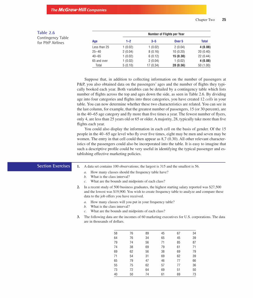
Suppose that, in addition to collecting information on the number of passengers atP&P, you also obtained data on the passengers’ ages and the number of flights they typi-cally booked each year. Both variables can be detailed by a contingency table which listsnumber of flights across the top and ages down the side, as seen in Table 2.6. By dividingage into four categories and flights into three categories, you have created 12 cells in yourtable. You can now determine whether these two characteristics are related. You can see inthe last column, for example, that the greatest number of passengers, 15 (or 30 percent), arein the 40–65 age category and fly more than five times a year. The fewest number of flyers,only 4, are less than 25 years old or 65 or older. A majority, 28, typically take more than fiveflights each year.
You could also display the information in each cell on the basis of gender. Of the 15people in the 40–65 age level who fly over five times, eight may be men and seven may bewomen. The entry in that cell could then appear as 8,7 (0.30). All other relevant character-istics of the passengers could also be incorporated into the table. It is easy to imagine thatsuch a descriptive profile could be very useful in identifying the typical passenger and es-tablishing effective marketing policies.
1. A data set contains 100 observations; the largest is 315 and the smallest is 56.
a. How many classes should the frequency table have?b. What is the class interval?c. What are the bounds and midpoints of each class?
2. In a recent study of 500 business graduates, the highest starting salary reported was $27,500and the lowest was $19,900. You wish to create frequency table to analyze and compare thesedata to the job offers you have received.
a. How many classes will you put in your frequency table?b. What is the class interval?c. What are the bounds and midpoints of each class?
3. The following data are the incomes of 60 marketing executives for U.S. corporations. The dataare in thousands of dollars.
58 76 89 45 67 3464 76 34 65 45 3979 74 56 71 85 8774 38 69 79 61 7169 62 56 38 69 7971 54 31 69 62 3965 79 47 46 77 6655 75 62 57 77 3673 72 64 69 51 5040 50 74 61 69 73
Table 2.6Contingency Tablefor P&P Airlines
Number of Flights per Year
Age 1–2 3–5 Over 5 Total
Less than 25 1 (0.02) 1 (0.02) 2 (0.04) 4 (0.08)25–40 2 (0.04) 8 (0.16) 10 (0.20) 20 (0.40)40–65 1 (0.02) 6 (0.12) 15 (0.30) 22 (0.44)65 and over 1 (0.02) 2 (0.04) 1 (0.02) 4 (0.08)
Total 5 (0.10) 17 (0.34) 28 (0.56) 50 (1.00)
Section Exercises

Version, Third Edition
26 Describing Data Sets
a. Construct a frequency table for the data. Exercise care in selecting your class intervals.Show the cumulative and relative frequencies for each class. What conclusions can youdraw from the table?
b. Present and discuss a more-than and a less-than cumulative frequency distribution.
4. From the data presented below, prepare a contingency table to evaluate 45 employees regard-ing their education level in years and the management level they currently hold. Divide educa-tion into three groups: group 1 for 10 to 12 years of education, group 2 for 13 to 15 years, andgroup 3 for 16 years and above. What patterns, if any, do you observe and what conclusionscan you reach?
Management Years of Management Years ofLevel Education Level Education
1 14 4 162 13 4 183 16 4 142 16 2 151 12 3 174 16 2 121 12 1 122 12 2 153 14 3 163 14 1 101 13 2 142 12 4 163 20 2 144 17 4 162 14 1 101 13 1 123 16 4 132 11 1 104 16 2 134 16 4 172 10 2 153 11 3 141 14
5. A production process for construction materials is designed to generate containers of threeweights: 10 pounds, 11 pounds, and 12 pounds. An examination of 40 of the containers recordstheir actual weights and their intended weights. A container is considered “defective” if its ac-tual weight differs by more than 0.5 pounds from its intended weight. Create a contingencytable with these data that indicates how many of the containers in each of the three weightgroups are within the allowable difference. Record the observations as “1” if defective and “2”if not defective. Can you detect any patterns? Does it appear that one weight group suffers alarger proportion of defects?
Actual Intended Actual IntendedWeight Weight Weight Weight
9.5 10 12.3 119.6 10 10.4 12
12.1 11 12.1 1011.2 12 10.0 1111.6 11 11.2 1012.3 12 9.9 12
(Continued)

Version, Third Edition
Chapter Two 27
Actual Intended Actual IntendedWeight Weight Weight Weight
9.6 10 9.6 1110.6 12 12.4 1011.0 11 11.2 1211.2 10 11.6 119.8 11 12.3 10
10.5 10 9.6 1211.9 12 10.6 1211.0 10 11.2 119.8 10 10.5 12
11.9 10 12.3 1010.4 12 12.1 1110.0 12 11.2 109.9 12 9.6 11
11.5 10 9.5 12
2.3 Pictorial DisplaysPictorial displays are also useful methods of describing data sets. A histogram places theclasses of a frequency distribution on the horizontal axis and the frequencies on the verti-cal axis. Figure 2.1 shows the histogram for the frequency distribution in Table 2.2. It re-veals details and patterns not readily discernible from the original raw data. The absoluteas well as the relative frequencies of each class are clearly illustrated.
Figure 2.1Histograms forP&P’s Passengers
Freq
uenc
y
20
15
10
5
050 60 70 80 90 100 110
Passengers
Figure 2.2P&P Performance
Bill
ions
of
dolla
rs
90
01993 1994 1995 1996 1997
Years
8070605040
302010
RevenueCosts

Version, Third Edition
28 Describing Data Sets
Figure 2.3Pie Chart
NeverLess than once a monthOnce a monthTwice a week3–4 times a weekEvery day
48%
10%
12%9%
8%
13%
How often employees take work home
Similar to a histogram, a bar chart can show absolute amounts or percentages fortwo or more values on the vertical axis. Figure 2.2 demonstrates the costs and revenuesfor P&P Airlines.
Figure 2.4High-Low-CloseChart for 15 Utilities
182
9
178
10 11 12 13
181
180
179
Dow
Jon
es I
ndex
of
15 u
tiliti
es
Selected day in June
Source: The Wall Street Journal.
Source: USA Today.
A pie chart is particularly useful in displaying relative (percentage) proportions of avariable. It is created by marking off a portion of the pie corresponding to each category ofthe variable. Figure 2.3 shows in percentages how often employees take work home fromthe office.
Financial data are often contained in a high-low-close chart. As the name suggests, itdisplays the highest value, the lowest value, and the closing value for financial instrumentssuch as stocks. Figure 2.4 is such a display based on data taken from The Wall Street Journalfor the Dow-Jones Index for 15 utilities over a five-day period based on the following data:
High Low Close
June 9 181.07 178.17 178.8810 180.65 178.28 179.1111 180.24 178.17 179.3512 182.79 179.82 181.3713 182.14 179.53 181.31

Version, Third Edition
Chapter Two 29
Sometimes called ticks and tabs, the upper end of the vertical line, or tick, marks offthe highest value that the index reached on that day; the lower end of the tick indicates thelowest value of the day. The closing value is shown by the little tab in between. Similar pre-sentations could be made for commodities and currencies traded on the world’s organizedexchanges.
John Tukey, a noted statistician, devised the stem-and-leaf design as an alternative tothe histogram to provide a quick visual impression of the number of observations in eachclass. Each observation is divided into two parts: a stem and a leaf separated by a verticalline. The precise design can be adjusted to fit any data set by identifying a convenient pointwhere the observations might be separated forming a stem and a leaf. Fractional valuessuch as 34.5, 34.6, 45.7, 45.8, and 56.2 might be divided at the decimal point producing astem-and-leaf, such as:
Stem Leaf
34 5, 645 7, 856 2
Notice that the stem and the leaf are placed in ordered arrays.If a single stem contains a large number of observations in its leaf, it is common to di-
vide it into two stems separated at the half-way point. Display 2.2 is the stem-and-leaf forour passenger data, provided by Minitab. The display contains three columns. The secondand third show the stem and the leaf, respectively. There are three observations in thefifties: 50, 57, and 59. The first column displays the depths, indicating the sum total of ob-servations from the top of the distribution for values less than the median (to be discussedlater in this chapter) or to the bottom of the distributions for values greater than the median.The depth in parentheses, (9), shows the number of observations in the stem containing themedian. For example, there are 19 observations from 50 up to 74 and 22 observations from80 up to the maximum observation of 102. Notice that there are two stems for the seventiesseparating the observations at the midpoint between 74 and 75.
Display 2.2Stem-and-Leaf for P&P
Character Stem-and-Leaf DisplayStem-and-leaf of pass N � 50Leaf Unit � 1.01 5 : 03 5 : 794 6 : 010 6 : 56789919 7 : 001122344(9) 7 : 56778899922 8 : 001233344412 8 : 5610 9 : 0123344 9 : 572 10 : 12
The leaf unit tells us where to put the decimal point. With leaf unit � 1.0, the first ob-servation is 50. Leaf unit � 0.1 would mean the first observation is 5.0 and leaf unit � 10would mean the first observation is 500.

Version, Third Edition
30 Describing Data Sets
6. Construct a stem-and-leaf design from the following unemployment rates in 15 industrializedcountries: 5.4 percent, 4.2 percent, 4.7 percent, 5.5 percent, 3.2 percent, 4.6 percent, 5.5 per-cent, 6.9 percent, 6.7 percent, 3.7 percent, 4.7 percent, 6.8 percent, 6.2 percent, 3.6 percent,and 4.8 percent.
7. Develop and interpret a histogram from the frequency table you constructed for Exercise 3.
8. Investors’ Report (July 1996) stated that last month people had invested, in millions of dollars,the following amounts in types of mutual funds: 16.7 in growth funds, 12.5 in income funds,28.2 in international funds, 15.9 in money market, and 13.9 in “other.” Construct a pie chartdepicting these data, complete with the corresponding percentages.
9. The changes from the previous month for investments in each of the funds in the previousproblem were, respectively, 2.3, 1.5, �3.6, 4.5, and 2.9. Construct a bar chart reflecting thesechanges.
Solved Problems1. A student organization is to review the amount students spend on textbooks each semester.
Fifty students report the following amounts, rounded to the nearest dollar.
$125 $157 $113 $127 $201165 145 119 148 158148 168 117 105 136136 125 148 108 178179 191 225 204 104205 197 119 209 157209 205 221 178 247235 217 222 224 187265 148 165 228 239245 152 148 115 150
a. Since 2c � 50 produces six classes, the interval for the frequency distribution is found as(highest � lowest)�6 � 265 � 104�6 � 26.8. An interval of 25 is used for convenience.This actually results in seven classes rather than the proposed six. No problem. If you setthe lower boundary for the first class at 100 (again, for convenience you could use 104),the table becomes:
Cumulative RelativeClass Interval Frequency M Frequency Frequency
100–124 8 112 8 0.16125–149 11 137 19 0.22150–174 8 162 27 0.16175–199 6 187 33 0.12200–224 10 212 43 0.20225–249 6 237 49 0.12250–274 1 262 50 0.02
b. The histogram and stem-and-leaf display provided by Minitab are:
Section Exercises

Version, Third Edition
Chapter Two 31
Histogram of C1 N � 50
Midpoint Count112.0 8 ********137.0 11 ***********162.0 8 ********187.0 6 ******212.0 10 **********237.0 6 ******262.0 1 *
Stem-and-leaf of C1 N � 50Leaf Unit � 1.0
3 10 4588 11 35799
11 12 55713 13 6619 14 58888824 15 02778(3) 16 55823 17 88920 18 719 19 1717 20 14559911 21 710 22 124585 23 593 24 571 251 26 5
The three lowest amounts are $104, $105, and $108. There are eight students who paid be-tween $104 and $119. This corresponds to the frequency of the first class in the tableabove. The next highest is $125. The median is in the stem for $160.
2. On a scale of 1 to 4, with 4 being best, a consumer group rates the “social consciousness” of50 organizations classified as public (indicated by a “1” in the data below), private (indicatedby a “2”), or government controlled (indicated by a “3”).
Type Rating Type Rating
1 1 2 22 2 3 32 3 1 13 2 2 41 4 3 42 2 1 23 3 2 32 2 3 21 1 1 12 2 3 43 3 2 21 4 1 3
(Continued)

Version, Third Edition
32 Describing Data Sets
Type Rating Type Rating
1 2 3 12 3 2 43 1 3 23 2 1 12 3 2 31 2 3 22 1 1 13 4 2 42 4 1 13 1 2 21 2 3 33 4 1 22 1 2 1
a. Prepare a contingency table complete with column and row totals and percentages. Whatconclusions might you draw? Minitab produces the table seen here. Notice that onlytwo, or 4 percent, of the 15 public organizations received a rating of “4.” Exactly twicethat percentage of private and government organizations earned the highest rating. Ofthe 50 organizations, 14 percent of those receiving a “1” were public units. Of those re-ceiving a “1,” 53.85 percent were public. Many other facts are evident from an examina-tion of the table.
ROWS: Type COLUMNS: Rating
1 2 3 4 ALL
(Public) 1 7 5 1 2 1546.67 33.33 6.67 13.33 100.0053.85 29.41 10.00 20.00 30.0014.00 10.00 2.00 4.00 30.00
(Private) 2 3 7 5 4 1915.79 36.84 26.32 21.05 100.0023.08 41.18 50.00 40.00 38.006.00 14.00 10.00 8.00 38.00
(Government) 3 3 5 4 4 1618.75 31.25 25.00 25.00 100.0023.08 29.41 40.00 40.00 32.006.00 10.00 8.00 8.00 32.00
ALL 13 17 10 10 5026.00 34.00 20.00 20.00 100.00100.00 100.00 100.00 100.00 100.0026.00 34.00 20.00 20.00 100.00
CELL CONTENTS ––COUNT% OF ROW% OF COL% OF TBL

Version, Third Edition
Chapter Two 33
List of Formulas[2.1] 2c � n Determines the number of
classes in a frequency table
[2.2] Class interval for a frequencytable
Chapter Exercises10. Bill Bissey, vice president of Bank One in Indianapolis, has control over the approval of loans
for local business development. Over the past five years the largest loan was $1.2 million, andthe smallest was $10,000. He wishes to construct a frequency table with 10 classes. Whatwould the boundaries of the classes be? What would the class interval be?
11. Mr. Bissey also maintains records on personal savings accounts. Of the 40 new accountsopened last month, the current balances are:
$ 179.80 $ 890.00 $ 712.10 $ 415.00112.17 1,200.00 293.00 602.02
1,150.00 1,482.00 579.00 1,312.52100.00 695.15 287.00 1,175.00
1,009.10 952.51 1,112.52 783.001,212.43 510.52 1,394.05 1,390.00
470.53 783.00 1,101.00 666.66780.00 793.10 501.01 1,555.10352.00 937.01 711.11 1,422.03
1,595.10 217.00 1,202.00 1,273.01
Construct a frequency table with seven classes. Are you working with continuous data ordiscrete data? Explain.
12. Using the data from Exercise 11, construct and interpret a relative frequency table and a cumulative frequency table.
13. Using the data from Exercise 11, construct a histogram.
14. Using the data from Exercise 11, construct a bar chart showing the percentages in each class.
15. Profits and losses for the 50 largest firms (by sales) on the Fortune 500 list for 1992 aregiven below in millions of dollars. The lowest value is a loss of $4,453 million (�4453),and the highest is a gain of $5,600 million. Construct a frequency table with the appropriatenumber of classes.
CI �Largest value � Smallest value
The number of desired classes

Version, Third Edition
34 Describing Data Sets
$ –4,453 $ –795 $ 423 $ 184 $ 975,600 1,567 454 258 939
–2,258 1,773 709 535 460–2,827 1,484 –578 1,461 –387
2,636 20 368 601 –4041,920 –1,021 755 –273 633,006 1,080 –732 1,681 3081,403 17 –617 –142 731,294 311 1,154 454 971,293 942 –1,086 2,056 505
16. As a private economic consultant, you find it necessary to faithfully read The Wall StreetJournal to remain current in your professional field. A recent report in The Wall Street Journalshowed the following data for percentages of executives in 42 top U.S. corporations sufferingfrom drug abuse problems.
5.9 8.8 14.3 8.3 9.1 5.1 15.317.5 17.3 15.0 9.3 9.9 7.0 16.710.3 11.5 17.0 8.5 7.2 13.7 16.312.7 8.7 6.5 6.8 13.4 5.5 15.28.4 9.8 7.3 10.0 11.0 13.2 16.39.1 12.3 8.5 16.0 10.2 11.7 14.2
a. Construct a stem-and-leaf design.b. Construct the corresponding histogram.c. Construct the frequency distribution and find the class midpoints.d. Construct the relative frequency distribution.
17. The following data regarding where Americans spend their vacations were recently publishedin Travel and Leisure: city 31 percent; ocean 26 percent; lake 5 percent; mountains 10 per-cent; state and national parks 6 percent; small rural town 22 percent. As director of the tourismboard for your state, it is your job to present these data in a pie chart.
18. Big Al, the local loan shark, currently has 120 outstanding accounts payable. Big Al’s accoun-tant informs him that of the 25 accounts in the $0 to $4,999 range, 10 are due, 5 are overdue,and the rest are delinquent, placing the debtor in danger of being visited by Big Al’s enforcer.Of the 37 in the $5,000 to $9,999 range, 15 are due, 10 are overdue and the rest are delin-quent. There are 39 in the $10,000 to $14,999 that show 11 are due, 10 are overdue, and therest are delinquent. Of the remaining accounts, in the $15,000 and up range, 5 are due, 7 areoverdue, and the rest are delinquent. Big Al wants to see a contingency table for these ac-counts. Interpret their significance by citing a few of the statistics you feel are most importantand revealing.
19. The Dow Jones averages for 30 industrial stocks reported the following values in June of1997. Construct a high-low-close chart based on these data.
High Low Close
June 2 6119.31 6081.79 6093.353 6123.58 6084.82 6101.714 6144.15 6084.64 6099.405 6148.12 6111.13 6124.47

Version, Third Edition
Chapter Two 35
20. Newsweek (August 26, 1996) reported percentages of various drugs preferred by those eighthgraders who had used drugs, and the percentage change since 1991 in the use of those drugs.Use the data on the 1996 rates of usage to create a pie chart and those on percentage changesto form a bar chart. Comment on the results.
Drug of Choice 1996 Usage Rate Percentage Change Since 1991
Crack 2.7% 108%Heroin 2.3 92Marijuana 19.5 95Cocaine 4.2 83Cigarettes 46.0 5Alcohol 25.3 �5
21. As a class project, a junior marketing student surveyed 20 local businesses in Peoria, Illinois,concerning their preference for a new product. Their responses were recorded as a “1” if theyliked the product, a “2” if they disliked it, and a “3” if they had no opinion. Annual sales lev-els for the stores were also recorded as a
1 if sales were less than $50,0002 if sales were $50,000 but less than $100,0003 if sales were $100,000 but less than $200,0004 if $200,000 or more
Construct a contingency table based on the data shown here. What conclusions can you reach?
Opinion Sales Opinion Sales
1.00 4.00 3.00 1.001.00 4.00 2.00 1.003.00 3.00 3.00 2.001.00 4.00 3.00 4.003.00 1.00 1.00 4.003.00 1.00 1.00 4.003.00 1.00 1.00 4.001.00 2.00 3.00 4.002.00 3.00 2.00 4.001.00 4.00 3.00 1.00
Computer ExerciseElizabeth Dunham is executive director of personnel operations for Minor Maturity Fashions, aclothing manufacturer that targets young women. She has collected data on weekly sales in hundredsof dollars over the past 100 weeks as well as payroll costs in thousands of dollars over the same pe-riod. However, Ms. Dunham is somewhat overwhelmed by the sheer volume of numbers she has ather disposal and is in need of assistance in organizing these data in some meaningful manner. Shemust gain some impression as to the nature of sales and payroll costs so that important informationmay be obtained for the forthcoming meeting of the board of directors. She also needs some adviceregarding what features of these important variables are most meaningful.
Access the file MINOR and provide Ms. Dunham with all relevant frequency distributions andpictorial displays your software might generate. You may have to create some of these descriptive

Version, Third Edition
From the Stage to Real LifeOn the Internet you can visit several national car rental companies and “Shopper’s Guides”to compare car rental prices and make reservations. A selection of these sites is the fol-lowing:
Shopping services:
Breeze Net’s Guide to Airport Rental Cars www.bnm.com
Car Rental Shopper’s guide www.rent-cars.com
36 Describing Data Sets
tools by hand if your software is not sufficiently flexible. Prepare a statistical report as detailed inAppendix I. Include all important parts of the statistical report including the executive summary andyour conclusions and recommendations.
C U R T A I N C A L L
City Rate City Rate City Rate
Miami 85 Houston 58 San Diego 89Houston 68 Phoenix 65 New Orleans 79New Orleans 65 Houston 63 Miami 62Miami 50 Phoenix 52 New Orleans 96Miami 102 Houston 87 Miami 98New Orleans 84 Houston 69 New Orleans 87Miami 110 Miami 85 Houston 69Phoenix 85 Phoenix 64 New Orleans 81Houston 95 New Orleans 97 Houston 62Phoenix 58 Phoenix 69 Phoenix 59Houston 59 New Orleans 74 Houston 63Phoenix 51 Phoenix 87 New Orleans 62New Orleans 76 Houston 67 New Orleans 52
In the opening case youwere to describe and char-
acterize the data you have collected on carrental rates for your long-awaited springbreak. Based on these data for daily rentalcharges from several companies in eachcity, prepare a detailed report describingyour findings. Include as many of the toolsdiscussed in this chapter as possible. Pro-
vide pictorial displays showing the averagecosts for each city as a percentage of theaverage cost of all cities.
Construct a contingency table showingeach of the cities in the columns. Divide thedata on rates into 3 to 5 groupings for therows. Include column and row percentagesand totals much as you did in Solved Prob-lem 2.

Version, Third Edition
Chapter Two 37
National car rental companies:
Alamo www.goalamo.com
Avis www.avis.com
Budget www.budgetrentacar.com
Hertz www.hertz.com
Thrifty www.thrifty.com
Using actual price information obtained from these Internet sites, redo the contingencytable you constructed in the Curtain Call exercise. Which of the cities of Miami, Houston,Phoenix, or New Orleans does the largest number of rental car companies service? Whichoffers the widest range of prices?

Version, Third Edition
38
C H A P T E R3Measures of CentralTendency and Dispersion

Version, Third Edition
39
Measures of Central Tendency and Dispersion
Central tendencies
Mean
Median
Mode
Weighted mean
Geometric mean
Grouped data
Range
Variance and standard deviation
Percentiles
Grouped Data
Ungrouped dataUngrouped data
Dispersion
Mean
Median
Mode
Variance and standard deviation
Chebyshev's Theorem SkewnessEmpirical rule Coefficient of variation
Related Concepts
Chapter BlueprintThis chapter illustrates how an entire data set can be described with only a few numbers. You will seehow useful measures of central tendency and measures of dispersion can be in statistical analysis.

Version, Third Edition
3.1 IntroductionData, like students, often congregate around their favorite gathering spots. Students seemto flock to places such as football games; frat houses; popular bars and other wateringholes; and, on rare occasions, even the library. Similarly, numbers seem to enjoy eachother’s company and are prone to collect around some central point referred to as the mea-sure of central tendency or, more commonly, as simply the average. A measure of centraltendency locates and identifies the point around which the data are centered.
A large data set can be quickly described in a succinct manner with a single number. Ifyour professor tells you that the class average on the last statistics test was a 95, that tellsyou something. If you are told that the average was a 35, that tells you something entirelydifferent.
40 Measures of Central Tendency and Dispersion
S E T T I N G T H E S T A G EFortune (February 17,1997) reported the aver-age annual returns for
three equity funds (Venture, Equity, andGrowth) offered by Janus Funds, a largemutual fund company. As an investment an-alyst you are assigned the task of analyzingJanus’s operations. To complete this jobassignment you must prepare a descriptiveaccount of the performance of the threefunds shown in the chart.
As the graph shows, the returns oneach of these funds have varied consider-ably over the years. There are many consid-erations that you must make in your ana-lysis, and your immediate supervisor has
stressed the importance of a thorough andprecise presentation.
Many questions arise as to just howyou might proceed. As this chapter reveals,there are many descriptive tools of statisti-cal analysis that you can use to develop youranalysis. Each tool plays an important rolein providing valuable information. Descrip-tive statistics such as average returns andmeasures of dispersion will be very useful.
In this chapter we will examine manyof the descriptive tools commonly used toconvey valuable information in a conciseand informative manner. Such practices re-duce uncertainty and greatly facilitate thedecision-making process.
Percentage Returns—Janus Funds
1994 1995 1996
30
25
20
15
10
5
0
VentureIncomeGrowth

Version, Third Edition
Chapter Three 41
In addition, measures of dispersion indicate the extent to which the individual obser-vations are spread out around their center point. They measure the dispersion or variabilityof the data and reflect the tendency of the individual observations to deviate from that cen-ter point.
3.2 Measures of Central Tendency for Ungrouped DataThere are three common methods of identifying the center of a data set: the mean, the me-dian, and the mode. Their calculation and interpretation will depend on the definition of“center.” In each case they locate the point around which the data are clustered.
A. The MeanThe mean, or arithmetic mean, is the measure of central tendency commonly thought of asthe average. To compute the mean of your last 10 statistics tests you simply add them upand divide by 10.
Arithmetic Mean The measure of central tendency normally thought of as theaverage.
The mean of a population is the parameter m (pronounced mu). If there are N observationsin the population data set, the mean is calculated as:
Population mean [3.1]
The Greek capital letter S is the summation sign telling you to add all the observationsfrom 1 to N. The Xi denotes the individual observations. For simplicity’s sake, the subscriptand superscript will hereafter be dropped and the summation sign will appear by itself assimply S.
The mean of a sample is a statistic (read X-bar). With n observations in the sampledata set, the mean is determined as:
Sample mean [3.2]
Presume that a sample of monthly sales revenues in thousands of dollars for fivemonths is found to be 56, 67, 52, 45, and 67. The mean is calculated as
X �56 � 67 � 52 � 45 � 67
5� 57.4
X �X1 � X2 � X3 �≥� Xn
n�
�n
i�1
Xi
n
X
m �X1 � X2 � X3 �≥� XN
N�
�N
i�1
Xi
N

Version, Third Edition
42 Measures of Central Tendency and Dispersion
B. The MedianThe median is sometimes referred to as the positional average, because it lies exactly in themiddle of the data set after the observations have placed into an ordered array. One-half ofthe observations will be above the median, and one-half will be below the median.
Median The middle observation after the data have been put into an ordered array.
If the data set has an odd number of observations, the median position is found as
[3.3]
Given our sample of sales revenues above, we must first place the data in an ordered array:
45, 52, 56, 67, 67
The position of the median value becomes
or the third position. From the ordered array above it can be seen that this value is 56.With a data set containing a even number of observations, it is necessary to average the
middle two values. If revenues for a sixth month of 35 is added to our data set the orderedarray becomes 35, 45, 52, 56, 67, 67. The median position is
or the third and one-half position. The two values in the third and fourth positions are thenaveraged to yield a median of 52 � 56 � 54. This means that, in one-half of the months,sales were below $54,000, and, in one-half of the months, revenues exceeded that amount.
C. The ModeThe modal observation is that observation that occurs with the greatest frequency. Usingour six observations above of 35, 45, 52, 56, 67, 67, the mode is 67. If a seventh observa-tion of 56 were added, the data set would be bimodal, with modes of 56 and 67.
Example 3.1 Measures of Central TendencyThe February 17, 1997, issue of Fortune reported the 1996 profits of several Fortune 500companies in millions of dollars, including:
Exxon $7,510 General Electric $7,280Philip Morris 6,246 IBM 5,429Intel 5,157 General Motors 4,289
Median position �6 � 1
2� 3.5
Median position �5 � 1
2� 3
Median position �n � 1
2

Version, Third Edition
Chapter Three 43
Calculate the three measures of central tendency.
Solution: Mean: Treating the data as a sample, we have
Median: The data must first be put in an ordered array. If the data are not ordered, the po-sition found using Formula 3.3 is meaningless.
4,289, 5,157, 5,429, 6,246, 7,280, 7,510
The median position is (n � 1)�2 � 3.5. The median is the average of the third and fourthvalues: 5,429 � 6,246 � 5,837.5.
Mode: This data set has no mode since all the observations occurred with equal frequency.
Interpretation: The mean and median identify the center of the data set around which the observations arelocated.
D. The Weighted MeanIn our discussion of the mean, we assumed that each observation was equally important.However, in certain cases you may want to give some observations greater weight. For ex-ample, if your statistics professor threatens to count the final exam twice as much as theother tests when determining your final grade, then the score you get on the final must begiven twice as much weight. That is, it must be counted twice in figuring your grade. Thisis exactly what the weighted mean does using Formula 3.4.
[3.4]
where is the weighted meanX is the individual observationsW is the weight assigned to each observation
Assume you scored 89, 92, and 79 on the hour exams, and 94 on the final exam. Thesescores and their respective weights are reflected in Table 3.1. Formula (3.4) yields
XW ��XW
�W�
448
5� 89.6
XW
XW ��XW
�W
X �7,510 � 7,280 � 6,246 � 5,429 � 5,157 � 4,289
6� 5,985
Table 3.1Calculation of theWeighted Mean
Grade (X) Weight (W ) XW
89 1 8992 1 9279 1 7994 2 188
5 448
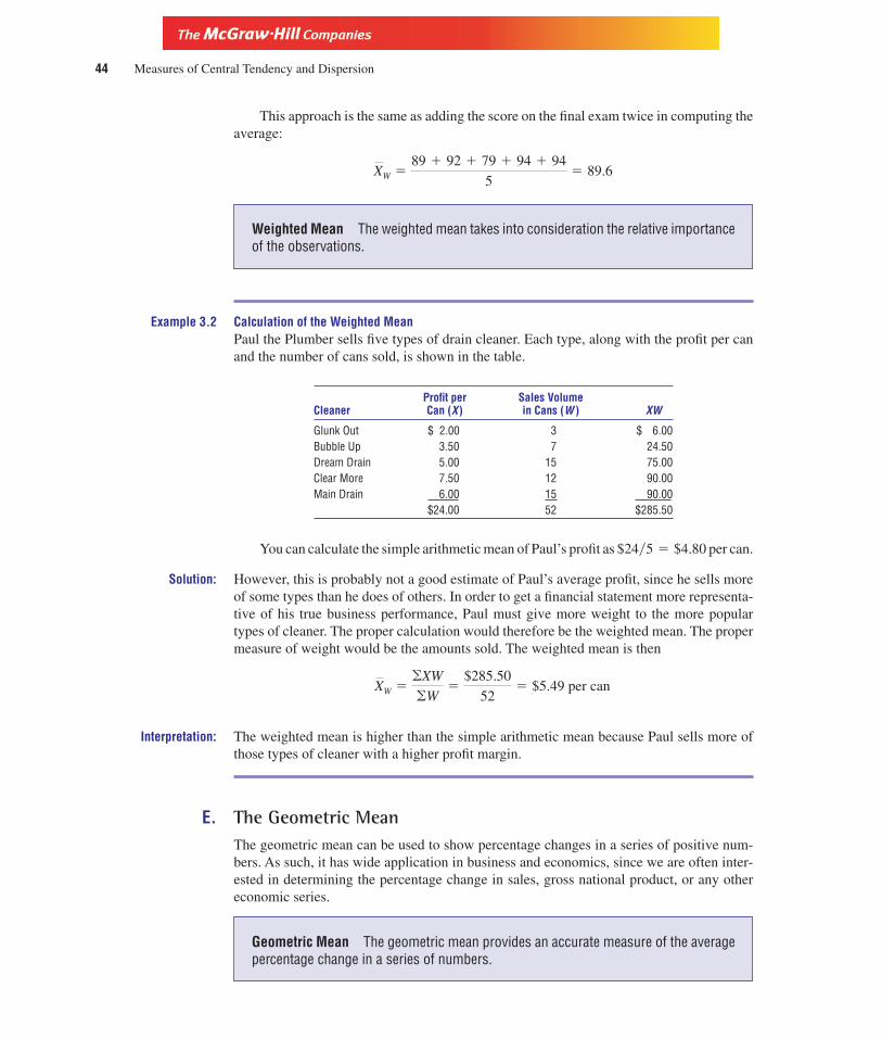
Version, Third Edition
44 Measures of Central Tendency and Dispersion
This approach is the same as adding the score on the final exam twice in computing theaverage:
Weighted Mean The weighted mean takes into consideration the relative importanceof the observations.
Example 3.2 Calculation of the Weighted MeanPaul the Plumber sells five types of drain cleaner. Each type, along with the profit per canand the number of cans sold, is shown in the table.
Profit per Sales VolumeCleaner Can (X ) in Cans (W ) XW
Glunk Out $ 2.00 3 $ 6.00Bubble Up 3.50 7 24.50Dream Drain 5.00 15 75.00Clear More 7.50 12 90.00Main Drain 6.00 15 90.00
$24.00 52 $285.50
You can calculate the simple arithmetic mean of Paul’s profit as $24�5 � $4.80 per can.
Solution: However, this is probably not a good estimate of Paul’s average profit, since he sells moreof some types than he does of others. In order to get a financial statement more representa-tive of his true business performance, Paul must give more weight to the more populartypes of cleaner. The proper calculation would therefore be the weighted mean. The propermeasure of weight would be the amounts sold. The weighted mean is then
Interpretation: The weighted mean is higher than the simple arithmetic mean because Paul sells more ofthose types of cleaner with a higher profit margin.
E. The Geometric MeanThe geometric mean can be used to show percentage changes in a series of positive num-bers. As such, it has wide application in business and economics, since we are often inter-ested in determining the percentage change in sales, gross national product, or any othereconomic series.
Geometric Mean The geometric mean provides an accurate measure of the averagepercentage change in a series of numbers.
XW ��XW
�W�
$285.50
52� $5.49 per can
XW �89 � 92 � 79 � 94 � 94
5� 89.6

Version, Third Edition
Chapter Three 45
The geometric mean (GM) is found by taking the nth root of the product of n numbers.Thus,
[3.5]
Most handheld calculators can compute the nth root of any number.The geometric mean is most often used to calculate the average percentage growth rate
over time of some given series. To illustrate its application in a business setting, considerthe revenue figures in Example 3.3 for White-Knuckle Airlines, P&P’s main competitor,over the past five years.
Example 3.3 The Geometric MeanThe CEO for White-Knuckle Airlines wishes to determine the average growth rate in rev-enue based on the figures in the table. If the average growth rate is less than the industryaverage of 10 percent, a new advertising campaign will be undertaken.
Revenues for White-Knuckle Airlines
Percentage ofYear Revenue Previous Year
1992 $50,000 — —1993 55,000 55�50 � 1.101994 66,000 66�55 � 1.201995 60,000 60�66 � 0.911996 78,000 78�60 � 1.30
Solution: It is first necessary to determine what percentage each year’s revenue is of the previousyear. In other words, the revenue in 1993 is what percentage of the revenue in 1992? Thisis found by dividing revenues in 1993 by those in 1992. The result, 1.10, reveals that 1993revenues are 110 percent of revenues in 1992. Percentages for the three remaining years arealso calculated. Taking the geometric mean of these percentages gives
Subtracting 1 in order to convert to an average annual increase yields 0.1179, or an 11.79percent average increase over the five-year-period.
The simple arithmetic average, on the other hand, is
or a 12.75 percent average change. We divide by 4, since there were four changes over thefive-year period.
However, if an average increase of 12.75 percent based on the simple arithmetic aver-age is applied to the series starting with $50,000, the results are
$71,667 � 1.1275 � $80,805
$63,563 � 1.1275 � $71,667
$56,375 � 1.1275 � $63,563
$50,000 � 1.1275 � $56,375
X �1.1 � 1.2 � 0.91 � 1.3
4�
4.51
4� 1.1275
GM � �4(1.10)(1.2)(0.91)(1.3) � 1.1179
GM � �n
X1 X2 X3≥Xn

Version, Third Edition
46 Measures of Central Tendency and Dispersion
Since $80,805 exceeds the $78,000 White-Knuckle Airlines actually earned, the12.75 percent increase is obviously too high. If the geometric mean growth rate of 11.79 per-cent is used, we get
This gives us a value of $78,088, which is much closer to the actual revenue of$78,000.
Interpretation: The geometric mean represents the average change over time. Since the growth rate ex-ceeds the industry average of 10%, the new advertising campaign will not be undertaken.
The geometric mean will always be less than the arithmetic mean except in the rarecase when all the percentage increases are the same. Then the two means are equal.
3.3 Comparing the Mean, the Median, and the ModeThe mean is the most common measure of central tendency. It lends itself handily to fur-ther algebraic manipulation and interpretation. Unfortunately, the mean is affected by ex-treme values, or outliers, and, unlike the median, can be drastically biased by observationswhich lie significantly above or below it.
For example, for the data 4, 5, 6, 6, 7, 8, the mean and the median are both 6 and rep-resent an excellent measure of the data’s center point. If the last observation were 80 in-stead of 8, the mean would become 18, but the median is still be 6. Since the median is notaffected by this extreme value, it better represents the six observations.
The mode is also less affected by a few atypical observations and remains 6 even if thelast value was 80. However, if there is no mode, or if the data set is bimodal, its use can beconfusing.
This does not imply that one measure is necessarily better than the others. The mea-sure you choose might depend on the nature of the data or the manner in which the data areused. For example, Land’s End, a popular retailer of camping equipment, would benefit lit-tle from the knowledge that the average size of the hiking boots it sold was 7.3492. Moreuseful in future business decisions would be knowledge of the modal size—recognizingthat it sold more boots of size 8 than any other.
However, assume that Land’s End wishes to market a new camping tent. The dimen-sions of the tent would depend, among other things, on the average height of adults. Expe-rience has shown that the mean serves quite well as a measure of central tendency whendealing with products that are built to conform to people’s height. The size of doorways,countertops in homes and retail businesses, and much of the furniture that is manufacturedis based on mean heights.
1. Your firm is introducing a new computer chip that is advertised to perform statistical calcula-tions much faster than those currently marketed. Twenty different calculations are made, pro-ducing the times in seconds seen below. Although you cannot misrepresent your product, you
$69,852 � 1.1179 � $78,088 � $78,000
$62,485 � 1.1179 � $69,852
$55,895 � 1.1179 � $62,485
$50,000 � 1.1179 � $55,895
Section Exercises

Version, Third Edition
Chapter Three 47
wish to present the results in the manner most favorable to your firm. Determine the mean, themedian, and the mode. Comment on the relative benefits of using each statistic.
3.2 4.1 6.3 1.9 0.65.4 5.2 3.2 4.9 6.21.8 1.7 3.6 1.5 2.64.3 6.1 2.4 2.2 3.3
2. As sales manager for Acme, Inc., you wish to calculate the measures of central tendency foryour firm’s profits levels over the last 12 months, given the following monthly profits inthousands of dollars:
$12.3 $14.3 $ 25.721.6 21.6 �12.822.3 18.0 23.1
�3.4 17.9 22.3
3. The plant director for Intel wants you to compare the mean wage rates for his plant in PaloAlto to that of a competitor’s in nearby San Jose. Of the 6,012 employees he supervises, 1,212earn $12.30 an hour, 650 are paid $15.50, 3,098 get $23.50, and the rest are paid $17.12. Ofthe 5,634 employees in the other plant, 1,654 earn $12.75, 815 receive $17.80, and the othersare paid $20.10. Write a brief report for the director detailing the information he wants.
4. A large firm selling sports equipment is testing the effect of two advertising plans on sales overthe last four months. Given the sales seen here, which advertising program seems to be pro-ducing the highest mean growth in monthly sales?
Month Plan 1 Plan 2
January $1,657 $4,735February 1,998 5,012March 2,267 5,479April 3,432 5,589
3.4 Measures of DispersionIn our efforts to describe a set of numbers, we have seen that it is useful to locate the cen-ter of that data set. But identifying a measure of central tendency is seldom sufficient. Amore complete description of the data set can be obtained if we measure how much the dataare dispersed around that center point. This is precisely what measures of dispersion do.They indicate how much the observations deviate around their mean.
Measures of Dispersion Measure the extent to which the individual observationsare spread out around their mean.
Take for example the three small data sets seen here.
Data Set 1 Data Set 2 Data Set 3
0,5,10 4,5,6 5,5,5

Version, Third Edition
48 Measures of Central Tendency and Dispersion
All three have a mean of five. Are we therefore to conclude that the data sets are similar? Ofcourse not. However, if we were told only their means, without seeing the observations, wemight conclude a similarity. A more accurate impression of the data sets would result if wecompared the degree to which the individual observations in each data set were dispersed orspread out around the mean of five. The observations in the first data set are quite scatteredout above and below the mean, whereas those in the second data set are comparatively closeto the mean. The first data set has a higher measure of dispersion than does the second. Thethird data set has no dispersion—all the observations are equal to the mean. Knowing this,we would be unlikely to mistakenly assume any similarity in the data sets merely on thebasis of their mean. Measures of dispersion in this sense are quite useful and informative.
A. The RangeThe simplest (and least useful) measure of dispersion is the range. The range is simply thedifference between the highest and the lowest observations. Its advantage is that it is easyto calculate. Its disadvantage is that it considers only two of the perhaps hundreds of ob-servations in the data set. The rest of the observations are ignored. The ranges of the threedata sets above are 10, 2, and 0 respectively.
B. The Variance and the Standard Deviation of a PopulationThe variance and its square root, the standard deviation, are much more useful measures ofdispersion. They provide a more meaningful measure of the extent to which the individualobservations are spread out around their mean.
The variance is the “mean of the squared deviation from the mean.” What does thatmean in English? It means that you (1) find the amount by which each observation deviatesfrom the mean, (2) square those deviations, and (3) find the average of those squared devi-ations. You then have the mean of the squared deviations from the mean.
Variance The mean of the squared deviations of the observations from their mean.
The variance for a population, s2 (read sigma squared) is
Populationvariance
[3.6]
where X1, X2, X3, . . . , XN are the individual observationsm is the population meanN is the number of observations
The standard deviation s is
Populationstandard deviation
[3.7]s � �s 2
��(Xi � m)2
N
s2 �(X1 � m)2 � (X2 � m)2 � (X3 � m)2 �≥� (XN � m)2
N
Version, Third Edition
Chapter Three 49
Notice that since we are working with a population, the mean is m, not as it is for a sam-ple, and the number of observations is N, not n as it is for a sample.
Standard Deviation The square root of the variance. It is an important measure ofthe dispersion of the data.
To illustrate, Chuckie Chambers sells five different insurance policies out of the trunkof his 1973 Plymouth. Their respective monthly premiums are $110, $145, $125, $95, and$150. The average premium is
The variance is found by: (1) subtracting the mean of $125 from each of the observations,(2) squaring these deviations, and (3) finding the average of these squared deviations. Fol-lowing these three steps yields
Despite the common use of the variance, it presents two problems. It is a rather largenumber relative to the observation. As you can see, it is several times greater than even thelargest observation. Due to its sheer size, the variance often becomes difficult to workwith.
An even more distressing problem results from the fact that since the deviationsare squared, the variance is always expressed in terms of the original data squared. InChuckie’s case, since he squared the deviations from the mean, it becomes 430 dollarssquared—a unit of measure that makes no sense. In most instances, the variance is ex-pressed in terms that have no logical meaning or interpretation.
However, both complications can be solved in a flash. Just find the standard deviations by taking the square root of the variance:
As easily as that, both problems are solved. You now have a much smaller number whichis easier to work with, and, more important, it is now expressed in dollars since you tookthe square root of dollars squared.
The concept of the standard deviation is quite important in business and economics.For example, in finance the standard deviation is used as a measure of the risk associatedwith various investment opportunities. By using the standard deviation to measure the vari-ability in rates of return offered by different investments, the financial analyst can gaugethe level of risk carried by each financial asset. Generally, the higher the standard deviationof the rate of return of a particular investment, the greater the degree of risk. Consider thefollowing example.
Example 3.4 Variance and Standard Deviation of a PopulationMarkus Boggs is manager of Nest Egg Investments. Recently, Markus was interested in therates of return over the past five years of two different mutual funds. Megabucks, Inc. showed
s � �430 � $20.74
� 430
s2 �(110 � 125)2 � (145 � 125)2 � (125 � 125)2 � (95 � 125)2 � (150 � 125)2
5
m �110 � 145 � 125 � 95 � 150
5� $125
X

Version, Third Edition
50 Measures of Central Tendency and Dispersion
rates of return over the five-year period of 12, 10, 13, 9, and 11 percent, while Dynamics Cor-poration yielded 13, 12, 14, 10, and 6 percent. A client approached Boggs and expressed aninterest in one of these mutual funds. Which one should Boggs choose for his client?
Solution: Notice that both funds offer an average return of 11 percent. Since both offer the same re-turn on the average, the safer investment is the one with the smaller degree of risk as mea-sured by the standard deviation. For Megabucks, Boggs finds
The standard deviation is
For Dynamics,
The standard deviation is therefore
Interpretation: Since Megabucks exhibits less variability in its returns and offers the same rate of return onthe average as does Dynamics, Megabucks represents the safer of the two investments andis therefore the preferred investment opportunity.
C. Variance and Standard Deviation for a SampleMake note: The previous examples relate to the variance and standard deviation for a pop-ulation. The symbols s2 and s are Greek letters typical of parameters.
Seldom do we calculate parameters. In most cases, we will instead estimate them bytaking a sample and computing the corresponding statistics. With that in mind, this sectionexamines the way in which we can calculate these important measures of dispersion as theyrelate to samples.
The variance and standard deviation for a sample represent measures of dispersionaround the mean. They are calculated quite similarly to those for a population. The samplevariance s2 is
Sample variance [3.8]
and the sample standard deviation is
Sample standard deviation [3.9]s � �s2
s2 ��(Xi � X )2
n � 1
s � �8 � 2.83%
s 2 �(13 � 11)2 � (12 � 11)2 � (14 � 11)2 � (10 � 11)2 � (6 � 11)2
5� 8
s � �2 � 1.41%
s2 �(12 � 11)2 � (10 � 11)2 � (13 � 11)2 � (9 � 11)2 � (11 � 11)2
5� 2

Version, Third Edition
Chapter Three 51
Notice that the mean in Formula (3.8) is expressed as , and not m, since we are workingwith samples. Furthermore, you divide by n � 1 rather than N because you have n � 1degrees of freedom, df � n � 1. The number of degrees of freedom in any statistical op-eration is equal to the number of observations minus any constraints placed on those ob-servations. A constraint is any value that must be computed from the observations.
For example, assume you are to choose n � 4 numbers which must average � 10.Under these conditions, you are free to pick any three numbers you want—say your hatsize, your age, and your IQ. Once those first three numbers are chosen, however, the fourthis predetermined if they are to average � 10. As Formula (3.8) illustrates, the varianceuses the value for which functions as a constraint and thereby reduces the degrees offreedom by 1. Hence, we divide by the number of observations, n, minus 1.
Another reason we divide by n � 1 is that a sample is generally a little less dispersedthan the population from which it was taken. There is therefore a tendency for the samplestandard deviation s to be a little less than the population standard deviation s. This is un-fortunate. Remember, we are trying to use the value of s as an estimation of s. However, swill consistently underestimate s. We must offset this condition by artificially inflating s bydividing by a slightly smaller number, n � 1, rather than n.
To illustrate the technique of determining these measures of dispersion for a sample,consider another problem Boggs has in the effort to help his clients make investmentdecisions.
Example 3.5 Variance and Standard Deviation for a sampleMr. Boggs wishes to determine the stability of the price of a particular stock. He decides tobase his judgment regarding stability on the standard deviation of the stock’s daily closingprice. Checking the financial pages, Boggs learns that the stock has been traded on the ex-change for quite some time and there are many closing prices dating back several months.Rather than using all these prices, Boggs decides to simplify his arithmetic and select arandom sample of n � 7 days. (Although 7 is probably too small a sample, it will serve ourpurposes for the moment.) He notes the closing prices of
$87, $120, $54, $92, $73, $80, and $63
Solution: Then, � $81.29 and
Interpretation: Boggs has estimated the mean closing price of the stock to be $81.29, with a tendency tovary above and below that price by $21.58. A further explanation of the use and interpreta-tion of the standard deviation is offered later in this chapter. However, keep in mind that
s � �465.9 � $21.58
s2 � 465.9 dollars squared
�(87 � 81.29)2 � (120 � 81.29)2 � … � (63 � 81.29)2
7 � 1
s2 ��(Xi � X)2
n � 1
X
XX
X
X

Version, Third Edition
52 Measures of Central Tendency and Dispersion
Boggs can always interpret the standard deviation of $21.58 as a measure of the tendencyof the closing prices to fluctuate around their mean of $81.29.
All these important statistics can be obtained from computer runs using various com-puter packages. Display 3.1 shows the Excell printout for our P&P data. Notice that themeasures of central tendency and dispersion are given along with other statistics we willdiscuss later.
Display 3.1Descriptive Statistics for P&P
Mean 78.36Standard Error 1.599938774Median 78.5Mode 83Standard Deviation 11.31327557Sample Variance 127.9902041Kurtosis -0.036918787Skewness -0.05225955Range 52Minimum 50Maximum 102Sum 3918Count 50
5. Two processes are used to produce computer disks. Problems have arisen regarding variationsin the sizes of these disks. Based on the sample data seen here for eight disk sizes in inches foreach process, explain which process you would advise if your objective is to minimize thedeviation in size around the mean.
Process 1 Process 2
3.41 3.22 3.81 3.263.74 3.06 3.26 3.793.89 3.65 3.07 3.143.65 3.33 3.35 3.51
6. Explain in your own words what the variance and standard deviation measure. Why is theircalculation slightly different for populations and samples?
7. An investment analyst suggests that you invest in Boomer Securities instead of ReliableStocks. Given the annual rates of return shown below for a sample of each investment, what doyou tell the analyst if you want to minimize your risk exposure?
Boomer Reliable
15.5% 3.6% 4.5% 6.2%21.7 27.2 5.5 7.2
�7.8 2.2 3.5 4.2�5.0 12.2 4.1
Section Exercises

Version, Third Edition
Chapter Three 53
8. Curly, Moe, and Larry sell life insurance for the Shemp Insurance Company. Mr. Shemp willpromote one of his salesmen to a management position based on sales performance. Hisdecision rests on which member of his sales force has (1) the highest average sales and (2) themost consistent sales record. Given the following weekly sample data for sales, which sales-man gets the promotion?
Curly Moe Larry
$ 0986 $1,265 $645 $893 $534 $5341,337 734 645 230 534 5342,745 245 734 415 534 5342,645 5,344 822 723 534 5343,658 4,867
3.5 Measures of Central Tendency and Dispersion forGrouped Data
In working with data that have been grouped into a frequency distribution, we do not knowwhat the individual observations are. In the frequency table for P&P’s passengers, Table 2.2,we know only that, on three days, somewhere between 50 and 59 passengers boarded anairplane. We do not have the exact counts on those three days. Without the specific values,the procedures shown above for calculating descriptive measures do not apply. Alternativeapproaches must be found. It should be kept in mind that computations made usinggrouped data are only approximations. Therefore, the ungrouped individual observationsshould be used when possible.
A. The MeanIn calculating the mean from grouped data, the assumption is made that the observations ineach class are equal to the class midpoint. Although this may be a rather heroic assumption,it probably all balances out, since it is likely that some of the observations exceed the mid-point while others fall below it. Given this assumption, we must take into consideration thefrequency and midpoints of each class when computing the mean using grouped data. For-mula 3.10 does just that.
Grouped mean [3.10]
where f is the frequency or number of observations in each classM is the midpoint of each classn is the sample size and equals the combined frequencies in all classes.
The frequency table for Pigs & People Airlines developed in Chapter 2 is repeated inTable 3.2 for your convenience, along with the midpoints for each class, which, as you re-member, are determined by averaging the upper and lower boundaries.
Using Formula (3.10), we can see that P&P flew a daily average of 78.7 passengers.
passengersXg �� fM
n�
3935
50� 78.7
Xg �� fM
n�
� fM
� f

Version, Third Edition
54 Measures of Central Tendency and Dispersion
Table 3.2FrequencyDistribution forPassengers
Class Frequency (f )(passengers) (days) M fM
50–59 3 54.5 163.560–69 7 64.5 451.570–79 18 74.5 1341.080–89 12 84.5 1014.090–99 8 94.5 756.0
100–109 2 104.5 209.050 3935.0
B. The MedianIf the data have been recorded in a frequency table, they cannot be placed in an orderedarray to calculate the median. As an illustration, the frequency table for P&P Airlines isgiven in Table 3.3.
We must first find the median class of the frequency distribution. The median class isthat class whose cumulative frequency is greater than or equal to n�2.
Since n is 50, we need to locate the first class with a cumulative frequency of 25 or more.The third class has a cumulative frequency of 28. The median can then be determined as
Median forgrouped data
[3.11]
where Lmd is the lower boundary of median class (70)F is the cumulative frequency of the class preceding the median class (10)fmd is the frequency of the median class (18)C is the class interval of the median class (10)
Using Formula (3.11), we obtain the median:
passengers
We can then conclude that on 25 days—one-half of the 50 days surveyed—fewer than78.33 passengers flew on P&P Airlines, and on the other 25 days, more than 78.33 passen-gers flew the friendly skies of P&P.
C. The ModeSince by definition the mode is the observation that occurs most often, it will be found inthe class with the highest frequency, called the modal class. To estimate the mode in thecase of grouped data, we use Formula (3.12).
Median � 70 � �50�2 � 10
18 �10 � 78.33
Median � Lmd � �n�2 � F
fmd� (C)
Table 3.3FrequencyDistribution forPassengers
Class f Cumulative Frequency
50–59 3 360–69 7 1070–79 18 2880–89 12 4090–99 8 48
100–109 2 50

Version, Third Edition
Chapter Three 55
Mode forgrouped data
[3.12]
where Lmo is the lower boundary of the modal classDa is the difference between the frequency of the modal class and the class
preceding itDb is the difference between the frequency of the modal class and the class
after itC is the class interval of the modal class
From Table 3.3, the mode is
passengers
D. Variance and Standard DeviationIf data are grouped into a frequency table, the variance and the standard deviation can becalculated as
Samplevariance ofgrouped data
[3.13]
and
Sample standarddeviation ofgrouped data
[3.14]
The passenger data for P&P Airlines will be used to illustrate.
Example 3.6 Measures of Dispersion with Grouped DataThe flight director for P&P requires information regarding the dispersion of the numbers ofpassengers. Decisions regarding scheduling and the most efficient size of planes to use de-pend on the fluctuation in the passenger load. If this variation in number of passengers islarge, bigger planes may be needed to avoid overcrowding on those days when the passen-ger load is extensive. The frequency table for P&P is as follows:
Class f(passengers) (days) M fM M 2 fM 2
50–59 3 54.5 163.5 2,970.25 8,910.7560–69 7 64.5 451.5 4160.25 29,121.7570–79 18 74.5 1,341.0 5,550.25 99,904.5080–89 12 84.5 1,014.0 7,140.25 85,683.0090–99 8 94.5 756.0 8,930.25 71,442.00
100–109 2 104.5 209.0 10,920.25 21,840.50n � 50 �fM � 3,935.0 �fM 2 � 316,902.50
s � �s2
s2 �� fM
2� nX
2
n � 1
Mode � 70 � � 18 � 7(18 � 12) � (18 � 7)� (10) � 76.47
Mode � Lmo � � Da
Db � Da� (C)

Version, Third Edition
56 Measures of Central Tendency and Dispersion
Solution: We calculated g in an earlier example as
Therefore, Formula (3.13) gives us
Interpretation: The flight director can now decide whether the planes currently in use can accommodatefluctuations in passenger levels as measured by a standard deviation of 12.14. If not, per-haps larger planes will be used to accommodate any overflow that might otherwise occuron those days with heavy traffic.
9. Daily absenteeism at your office seems to be increasing. Last year an average of 47.8 em-ployees were absent each day, with a standard deviation of 14.7 employees. A sample of datawas gathered for the current year and placed in the frequency table shown below. Calculatethe mean, the median, the mode, and the standard deviation for these data and compare themto those for the previous year. What conclusions do you reach?
Number of Employees Days That NumberAbsent Was Absent
20–29 530–39 940–49 850–59 1060–69 1270–79 1180–89 890–99 3
10. In the past, completion time for a certain job task in the offices at Harmon Electronics haveshown the following statistics in hours: a mean of 12.2, a median of 13.2, and a mode of14.5. The variance was 8.21. More recent data are reflected in the frequency table below.Mr. Harmon hires you as an outside consultant to evaluate changes in employee efficiency.Calculate the corresponding statistics based on these data, and prepare a brief report. Whatconclusions do you offer?
Hours to CompletionNumber of Times the Task
Took This Long
5 and under 7 47 and under 9 89 and under 11 12
11 and under 13 813 and under 15 515 and under 17 2
s � �147.31 � 12.14 passengers
s2 �316,902.50 � 50(78.7)2
49� 147.31 passengers squared
s2 �� fM
2� nX
2
n � 1
Xg �� fM
n�
3935
50� 78.7
X
Section Exercises

Version, Third Edition
Chapter Three 57
3.6 Other Measures of DispersionAlthough the variance and the standard deviation are the most useful measures of disper-sion in statistical analysis, there are other ways the dispersion of a data set might be mea-sured. These additional measures of dispersion are quartiles, deciles, and percentiles.
Every data set has three quartiles that divide it into four equal parts. The first quartileis that value below which 25 percent of the observations fall, and above which the remain-ing 75 percent can be found. The second quartile is right in the middle. One-half the ob-servations are below it and one-half the observations are above it; in this sense, it is thesame as the median. The third quartile is that value below which 75 percent of the obser-vations are located, and above which the remaining 25 percent can be found.
The determination of quartiles is often useful. Many graduate schools, for example,will admit only those students in the top 25 percent (third quartile) of their applicants. Cor-porations often wish to single out those plants whose poor production records place thembelow the bottom quartile. With only a little imagination, it is possible to envision numer-ous instances in which the determination of quartiles might prove beneficial.
Deciles separate a data set into 10 equal subsets, and percentiles produce 100 parts.The first decile is that observation below which 10 percent of the observations are found,while the remaining 90 percent are located above it. The first percentile is that value belowwhich 1 percent of the observations are located, and the rest are above it. A similar inter-pretation can be applied to the rest of the deciles and percentiles. Each data set has 9 decilesand 99 percentiles.
A percentile and its location in an ordered array are identified by means of subscripts.For example, the 15th percentile is indicated as P15, and its location in the ordered arrayis L15.
To illustrate the calculation of percentiles, assume that we have observations forthe number of shares for 50 stocks traded on the New York Stock Exchange, as shown inTable 3.4. Notice that the data have been placed in an ordered array. The location of the Pthpercentile is found as
Location of apercentile
[3.15]
where Lp is the location in the ordered array of the desired percentilen is the number of observationsP is the desired percentile
Assume that we wish to calculate the 25th percentile, P25, for the stocks in Table 3.4.We must first find its location in the ordered array.
� 12.75
L25 � (50 � 1)25
100
Lp � (n � 1)P
100
Table 3.4Numbers of SharesTraded on the NYSE(in 100’s)
3 10 19 27 34 38 48 56 67 744 12 20 29 34 39 48 59 67 747 14 21 31 36 43 52 62 69 769 15 25 31 37 45 53 63 72 79
10 17 27 34 38 47 56 64 73 80

Version, Third Edition
58 Measures of Central Tendency and Dispersion
The resulting value of 12.75 tells us that the 25th percentile is located 75 percent of the waybetween the 12th observation of 20 and the 13th observation of 21, or P25 � 20 � 0.75(21 � 20) � 20.75.
If we wish to calculate the 35th percentile, we find
The 35th percentile is 85 percent of the way between the 17th observation of 29 and the18th observation of 31, or P35 � 29 � (0.85)(31 � 29) � 30.7. Thus, 35 percent of theobservations are below 30.7, and the remaining 65 percent are above 30.7.
Returning to deciles and quartiles for a moment, note that the first decile is equal toP10, that the second decile is equal to P20, and so on. Additionally, the first quartile is thesame as P25, the second quartile equals P50, and P75 locates the third quartile. With that inmind, the calculation of deciles and quartiles becomes simply a matter of determining theappropriate percentiles according to the rules that we have just established.
A unique measure of dispersion is the interquartile range (IQR). The IQR is the dif-ference between the first quartile and the third quartile. That is, P75 � P25. One-half of theobservations lie within this range. It consists of the middle 50 percent of the observationsin that it cuts off the lower 25 percent and the upper 25 percent of the data points. As a re-sult, the IQR provides a measure of dispersion that is not heavily influenced by a few ex-treme observations. The interquartile range is illustrated in Figure 3.1.
� 17.85
L35 � (50 � 1)35
100
Figure 3.1The InterquartileRange Q1 Q2 Q3
IQR
middle 50%
Lower25%
Upper25%
Section Exercises 11. Define in your own words:
a. The 80th percentile.b. The fourth decile.c. The third quartile.
12. Using the data from Table 3.4, calculate and interpret:
a. The interquartile range.b. The median.c. The 50th percentile.d. The 70th percentile.e. The third decile.

Version, Third Edition
Chapter Three 59
3.7 Common Uses for the Standard DeviationAs we have emphasized, the standard deviation is useful for describing a data set by mea-suring the extent to which the individual observations are spread out around their mean.There are at least two additional applications for the standard deviation: (1) Chebyshev’sTheorem and (2) the Empirical Rule.
A. Chebyshev’s TheoremChebyshev’s Theorem (sometimes spelled Tchebysheff’s Theorem) was formulated by theRussian mathematician P. L. Chebyshev (1821–1894). It states that for any data set, at least1 � 1�K 2 percent of the observations lie within K standard deviations of the mean, whereK is any number greater than 1. Chebyshev’s Theorem is expressed as
Chebyshev’s Theorem [3.16]
Thus, for example, if we form an interval from K � three standard deviations abovethe mean to three standard deviations below the mean, then at least
of all the observations will be within that interval.
Example 3.7 Chebyshev’s Theorem Applied to Pigs and People AirlineOur earlier work in this chapter with the grouped data for P&P Airlines revealed a mean of78.7 passengers per day, with a standard deviation of 12.14. In order to schedule times fora new route P&P opened, management wants to know how often the number of passengersis within K � two standard deviations of the mean, and what that interval is.
Solution: If we move two standard deviations (2 � 12.14) � 24.28 passengers above and below themean of 78.7, we will have an interval of (78.7 � 24.28) � 54.42 to(78.7 � 24.28) � 102.98 passengers. We can then be certain that at least
of the time, the number of daily passengers was between 54 and 103.
Interpretation: On at least 75 percent of the days (that is, 75 percent of 50 equals 37 days), the number ofpassengers was between 54 and 103. This provides the management of P&P with valuableinformation regarding how many passengers to prepare for in terms of in-flight operations.
B. The Normal Distribution and the Empirical RuleMore important, the standard deviation can be used to draw certain conclusions if the dataset in question is normally distributed. The concept of a normal distribution is commonlyencountered in statistical analysis and is of considerable importance. A thorough discussion
1 �1
22 � 75%
1 �1
32 � 88.89%
1 � � 1
K 2�

Version, Third Edition
60 Measures of Central Tendency and Dispersion
of the normal distribution is presented in later chapters. However, an early introduction tothis all-important concept will allow us to demonstrate a practical use for the standard de-viation, and will set the basis for the more thorough investigation to come. A normal dis-tribution is a distribution of continuous (not discrete) data that produces a bell-shaped,symmetrical curve like that shown in Figure 3.2.
Figure 3.2A NormalDistribution
Freq
uenc
y of
obs
erva
tion
MeanMedianMode
f (x)
X (minutes)0 5 10 15 20
Assume that we have a large number of observations for the time, in minutes, that ittakes skiers to complete a particular run. If the data are normally distributed, a graph of thefrequency with which each observation occurs will take the shape of Figure 3.2. The ob-servations at each extreme will occur relatively infrequently, but those observations closerto the middle will occur with increasing frequency, thereby producing the bell-shaped sym-metrical curve. The modal observation, 10 in our case, is the one occurring with the great-est frequency and is therefore at the peak of the distribution. In a normal distribution, themean, median, and the mode are all equal.
Of importance, one-half of the observations are above the mean and one-half arebelow it. This means that one-half of the area under the curve is to the left of the mean, andone-half of the area under the curve is to the right of the mean.
To illustrate how the standard deviation applies to the normal distribution, assume1,000 skiers slalom down the bunny slope at Vail. The times for all skiers happen to be nor-mally distributed, with a mean of m � 10 minutes and a standard deviation of s � -2 minutes. The Empirical Rule tells us that if we include all observations within one stan-dard deviation of the mean (one standard deviation above the mean and one standarddeviation below the mean) we will encompass 68.3 percent of all the observations. That is,no matter what the mean is and no matter what the standard deviation is, we can be certainthat 68.3 percent of the observations lie within one standard deviation of the mean if the ob-servations are normally distributed.
Since the skiers averaged 10 minutes to complete the run, moving one standarddeviation (that is, 2 minutes) above and below this mean of 10 produces a range of 8 to12 minutes. Thus, according to the Empirical Rule, 683 (68.3 percent of the 1,000) skierstook between 8 and 12 minutes to get down the mountain.
Of course, if we move more than one standard deviation above and below the mean, wewill encompass a larger percentage of the observations. The Empirical Rule specifies that
68.3 percent of the observations lie within plus or minus one standard deviation ofthe mean.
95.5 percent of the observations lie within plus or minus two standard deviations ofthe mean.
99.7 percent of the observations lie within plus or minus three standard deviationsof the mean.
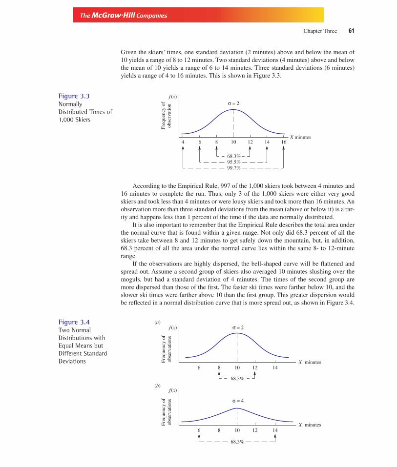
Version, Third Edition
Chapter Three 61
Given the skiers’ times, one standard deviation (2 minutes) above and below the mean of10 yields a range of 8 to 12 minutes. Two standard deviations (4 minutes) above and belowthe mean of 10 yields a range of 6 to 14 minutes. Three standard deviations (6 minutes)yields a range of 4 to 16 minutes. This is shown in Figure 3.3.
Figure 3.3NormallyDistributed Times of1,000 Skiers
Freq
uenc
y of
ob
serv
atio
n
68.3%95.5%99.7%
f (x)
X minutes4 6 10 12 168 14
σ = 2
Figure 3.4Two NormalDistributions withEqual Means butDifferent StandardDeviations minutes
f (x)
X6 10 128 14
σ = 2
68.3%
68.3%
f (x)
X6 10 128 14
minutes
σ = 4
Freq
uenc
y of
ob
serv
atio
nsFr
eque
ncy
of
obse
rvat
ions
(b)
(a)
According to the Empirical Rule, 997 of the 1,000 skiers took between 4 minutes and16 minutes to complete the run. Thus, only 3 of the 1,000 skiers were either very goodskiers and took less than 4 minutes or were lousy skiers and took more than 16 minutes. Anobservation more than three standard deviations from the mean (above or below it) is a rar-ity and happens less than 1 percent of the time if the data are normally distributed.
It is also important to remember that the Empirical Rule describes the total area underthe normal curve that is found within a given range. Not only did 68.3 percent of all theskiers take between 8 and 12 minutes to get safely down the mountain, but, in addition,68.3 percent of all the area under the normal curve lies within the same 8- to 12-minuterange.
If the observations are highly dispersed, the bell-shaped curve will be flattened andspread out. Assume a second group of skiers also averaged 10 minutes slushing over themoguls, but had a standard deviation of 4 minutes. The times of the second group aremore dispersed than those of the first. The faster ski times were farther below 10, and theslower ski times were farther above 10 than the first group. This greater dispersion wouldbe reflected in a normal distribution curve that is more spread out, as shown in Figure 3.4.
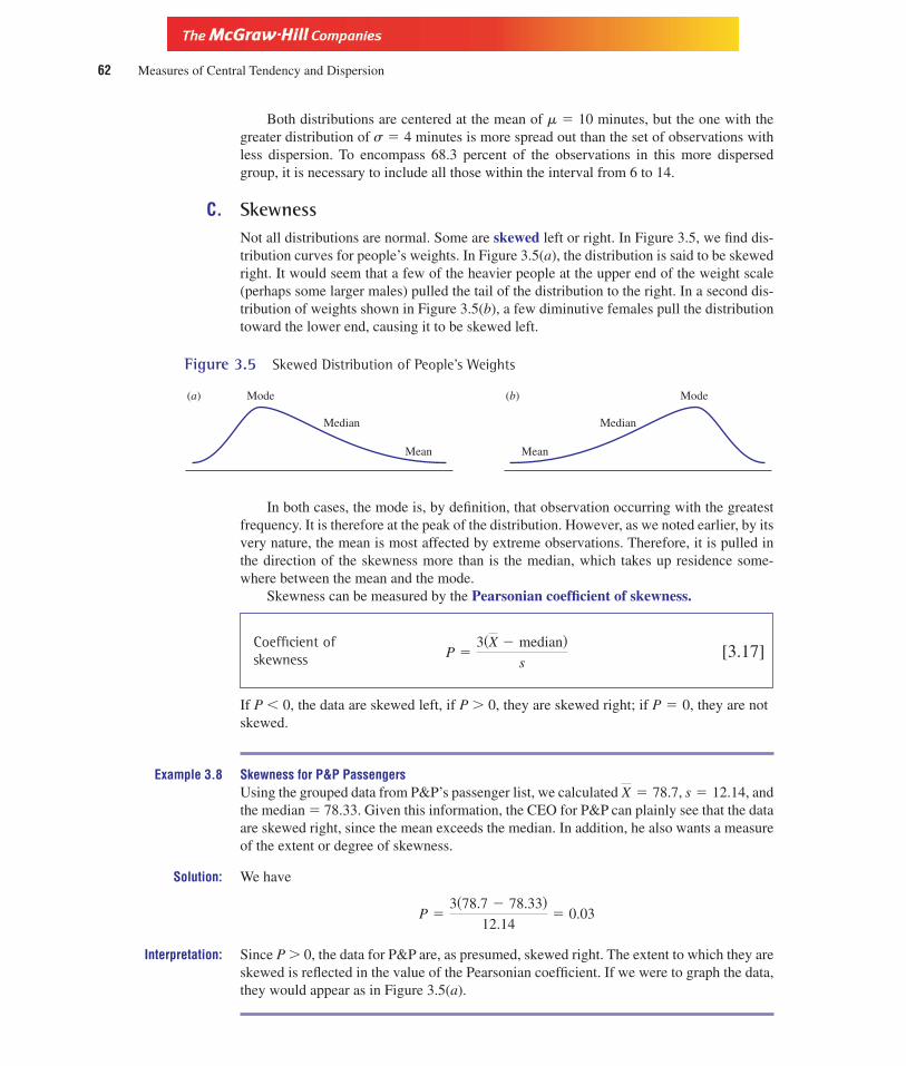
Version, Third Edition
62 Measures of Central Tendency and Dispersion
In both cases, the mode is, by definition, that observation occurring with the greatestfrequency. It is therefore at the peak of the distribution. However, as we noted earlier, by itsvery nature, the mean is most affected by extreme observations. Therefore, it is pulled inthe direction of the skewness more than is the median, which takes up residence some-where between the mean and the mode.
Skewness can be measured by the Pearsonian coefficient of skewness.
Coefficient ofskewness [3.17]
If P � 0, the data are skewed left, if P 0, they are skewed right; if P � 0, they are notskewed.
Example 3.8 Skewness for P&P PassengersUsing the grouped data from P&P’s passenger list, we calculated � 78.7, s � 12.14, andthe median � 78.33. Given this information, the CEO for P&P can plainly see that the dataare skewed right, since the mean exceeds the median. In addition, he also wants a measureof the extent or degree of skewness.
Solution: We have
Interpretation: Since P 0, the data for P&P are, as presumed, skewed right. The extent to which they areskewed is reflected in the value of the Pearsonian coefficient. If we were to graph the data,they would appear as in Figure 3.5(a).
P �3(78.7 � 78.33)
12.14� 0.03
X
P �3(X � median)
s
Figure 3.5 Skewed Distribution of People’s Weights
(a) Mode
Median
Mean
(b) Mode
Median
Mean
Both distributions are centered at the mean of m � 10 minutes, but the one with thegreater distribution of s � 4 minutes is more spread out than the set of observations withless dispersion. To encompass 68.3 percent of the observations in this more dispersedgroup, it is necessary to include all those within the interval from 6 to 14.
C. SkewnessNot all distributions are normal. Some are skewed left or right. In Figure 3.5, we find dis-tribution curves for people’s weights. In Figure 3.5(a), the distribution is said to be skewedright. It would seem that a few of the heavier people at the upper end of the weight scale(perhaps some larger males) pulled the tail of the distribution to the right. In a second dis-tribution of weights shown in Figure 3.5(b), a few diminutive females pull the distributiontoward the lower end, causing it to be skewed left.

Version, Third Edition
Chapter Three 63
D. Coefficient of VariationAs we have emphasized, an important use of the standard deviation is to serve as a measureof dispersion. However, certain limitations apply. When considering two or more distribu-tions that have significantly different means, or that are measured in different units, it isdangerous to draw conclusions regarding dispersion merely on the basis of the standard de-viation. It is like violating the old adage about comparing apples and oranges.
We must therefore often turn to the coefficient of variation (CV), which serves as arelative measure of dispersion. The coefficient of variation assesses the degree of disper-sion of a data set relative to its mean. It is computed by dividing the standard deviation ofa distribution by its mean, and multiplying by 100.
Coefficient ofvariation
[3.18]
The grouped data for P&P reported a mean of 78.7 passengers per day, with a standarddeviation of 12.14 passengers. Presume that P&P also collects data over the same time pe-riod for the number of miles flown by the airline and that the daily mean and standard de-viation prove to be 1,267.5 and 152.7, respectively. The higher standard deviation for milesflown might suggest that these data exhibit a far greater variation.
However, if we calculate the coefficient of variation for passengers, we find it to be
while that for miles is only
It is clear that, in comparing the variation in two vastly different data sets, it is wise to usethe coefficient of variation and not just the standard deviation.
13. A data set for the fill weights of 1000 bags of Happy Pooch dog food has a mean of 50pounds and a standard deviation of 2.3 pounds. The data are not known to be normallydistributed. The makers of Happy Pooch hope that at least 750 of those bags weigh between45.4 and 54.6 pounds. What assurance can you give them?
14. A normally distributed data set has a mean of 5,000 and a standard deviation of 450. Whatpercentage of the observations lie:
a. Between 4550 and 5450?b. Between 4100 and 5900?c. Between 3650 and 6350?d. Above 6350?e. Below 4550?
15. Shard Lumber cuts logs to a mean length of 20 feet, with a standard deviation of 3.5 feet. Ifthe cuts are normally distributed, what percentage of the logs are less than:
a. 16.5 feet?b. 13 feet?
CV �152.7
1267.5(100) � 12.05
CV �12.14
78.70(100) � 15.43
CV �s
X(100)
Section Exercises

Version, Third Edition
64 Measures of Central Tendency and Dispersion
16. Data on ages of 100 top executives for Fortune 500 firms reveal a mean age of 56.2 years anda standard deviation of 12.7 years. Their mean income is $89,432, with s � $16,097. Whichvariable, age or income, exhibits the greater variation?
17. If the median income in Exercise 16 is $87,567,
a. Are the data skewed right, skewed left, or normally distributed?b. What is the Perasonian coefficient of skewness?
Solved Problems1. Information Pays A 1996 issue of Inc. Technology reported that Information Please, a
new firm selling information over the Internet, recorded the number of “hits’’ it had on anhourly basis as 47, 52, 69, 72, 112, 36, 28, 68, 69, and 41. Presume that the manager wishesto evaluate these data on the basis of their measures of central tendency and measures ofdispersion.
The mean is
Given the ordered array 28, 36, 41, 47, 52, 68, 69, 69, 72, 112, the median position is
and the median is the average of the fifth and sixth observations or 52 � 68�2 � 60. Themode is the observation that occurred most frequently, 69. The variance is
and the standard deviation is .
2. Weighing In Members of the Heart-to-Heart Health Club are charged dues on the basis oftheir average weight. Of the 60 members, 12 weighed 110 pounds, 25 weighed 120 pounds,18 tipped the scale at 150 and the rest registered 180 pounds. If the members must pay $5 foreach pound they weigh on the average, how much must each fork over?
Since each weight category contained a different number of members, the weightedmean is necessary.
Pounds (X ) Number of Members (W ) XW
110 12 1320120 25 3000150 18 2700180 5 900
60 ��W 7920 ��XW
Thus, each member must pay 132 � 5 � $660.
3. Growing Pains Employee dissatisfaction at Bates Electronics is reflected in the number ofofficial complaints over the past four months: 23, 41, 37 and 49. Based on these data, what isthe average monthly increase in complaints?
Xw ��XW
�W� 132 pounds
�584.933 � 24.185
s 2 ��(Xi � X )2
n � 1�
5264.4
9� 584.933
Median position �n � 1
2� 5.5
X ��Xi
n�
594
10� 59.4

Version, Third Edition
Chapter Three 65
The geometric mean, whose job it is to determine average percentage change over time,requires that we first determine what percentage each number is of the previous month:
Month Complaints Percentage of Previous Month
1 23 —2 41 1.783 37 0.904 49 1.32
Then,
Then, 1.28 � 1.00 � 28 percent mean monthly increase in complaints.
4. People Who Care Statisticians for the Meals on Wheels program, which brings hot mealsto shut-ins, want to evaluate their services. The number of daily meals they provide is shownin the frequency table below.
Number of Meals Per Day Number of Days M fM fM2
0–5 3 2.5 7.5 18.756–11 6 8.5 51.0 433.50
12–17 5 14.5 72.5 1,051.2518–23 8 20.5 164.0 3,362.0024–29 2 26.5 53.0 1,404.5030–35 3 32.5 97.5 3,168.75
27 445.5 9,438.75
The mean, median, and modal number of meals are
The variance and standard deviation are
s � �80.31 � 8.96 meals
� 80.31
�9438.75 � 27(16.5)2
27 � 1
s2 �� fM
2� nX
2
n � 1
� 20 meals
� 18 � � 3
3 � 6 �(6)
Mode � Lmo � � Da
Da � Db�(c)
� 17.4 meals
� 12 � � 27�2 � 9
5 �(6)
Median � Lmd � � n�2 � F
fmd�(c)
Xg �� fM
n�
445.5
27� 16.5 meals per day
GM � �n(Xi)(X2) . . . (Xn) � �3
(1.78)(0.9)(1.32) � 128

Version, Third Edition
66 Measures of Central Tendency and Dispersion
List of Formulas
[3.1] Population mean.
[3.2] Sample mean.
[3.3] Determines the positionof the median in anordered array.
[3.4] Determines the weighted mean.
[3.5] Calculates the averagepercentage change.
[3.6] Variance for a population.
[3.7] Population standard deviation.
[3.8] Sample variance.
[3.9] Sample standard deviation.
[3.10] Mean for grouped data.
[3.11] Median for grouped data.
[3.12] Mode for grouped data.
[3.13] Sample variance forgrouped data.
[3.14] Standard deviation ofgrouped data.
[3.15] Location of a percentile.
[3.16] Chebyshev’s Theorem.
[3.17] Coefficient of skewness.
[3.18] Coefficient of variation.CV �s
X(100)
P �3(X � median)
s
1 � � 1
K2�
Lp � (n � 1)P
100
s � �s2
s2 �� fM
2� nX
2
n � 1
Mode � Lmo � � Da
Da � Db� (C)
Median � Lmd � � n�2 � F
fmd� (C)
Xg �� fM
n
s � �s2
s2 ��(Xi � X)2
n � 1
s � �s 2
s2 ��(Xi � m)2
N
GM � �n(X1)(X2) . . . (Xn)
Xw ��XW
�W
Median position �n � 1
2
X �X1 � X2 � X3 �≥� Xn
n�
�n
i�1
Xi
n
m �X1 � X2 � X3 �≥� XN
N�
�N
i�1
Xi
N

Version, Third Edition
Chapter Three 67
Chapter Exercises18. Stock prices are quoted in eighths of dollars such that, for example, 5 1�8 is $5.125, 5 1�4 is
$5.25, 5 3�8 is $5.375, and so on up to 5 7�8, which is $5.875. Below is a sample of sevenclosing prices of stocks taken from The Wall Street Journal of October 8, 1997.
Wal-Mart 27 3�8 General Mills 69 7�8Disney 42 5�8 Toys R Us 38 5�8Mobil 69 7�8 Dow Jones 29 1�4General Motors 39 1�2
a. Calculate the mean, the median, and the mode. Interpret each statistic. What does eachtell you? Why are they different if they are all averages?
b. Calculate and interpret the variance and the standard deviation.c. Calculate and interpret the interquartile range.d. Calculate and interpret the fortieth percentile.
19. The Snowflake markets ski boots in San Luis Obispo, California. Of the last 100 pairs sold,4 were size 9, 33 were size 9 1�2, 26 were size 10, 29 were size 10 1�2, and 8 were size 13.Comment on the use of the mean, median, and mode as measures of central tendency andthe use of each in making decisions regarding sizes to hold in inventory. Calculate eachmeasure.
20. As interest rates fell in early 1997, a sample of mortgage rates for 15-year mortgages at locallending institutions in Peoria, Illinois, was found to be
7.1%, 7.3%, 7.0%, 6.9%, 6.6%, 6.9%, 6.5%, 7.3%, 6.85%
a. Calculate and interpret the mean, the median, and the mode.b. Are these data skewed left, or right, or are they normally distributed? Calculate the
Pearsonian coefficient as a measure of the skewness.c. Calculate and interpret the variance and the standard deviation.
21. A survey of lending institutions in an urban center near Peoria (see previous problem)revealed mortgage rates of
7.1%, 7.3%, 6.3%, 6.7%, 6.8%, 6.85%, 7.5%
a. Are mortgage rates higher in Peoria or the other urban center?b. Which city seems to have the most consistent rates among institutions?c. Calculate and interpret the Pearsonian coefficient of skewness.
22. Alan Munday manufactures a paint sealant for automobiles in the Denver area. He uses fourdifferent chemicals in the production process. To make his product, Munday must use 2 gallonsof calcimine which costs $2.50 per gallon, 1�2 gallon of kalsolite at $1.25 per gallon, 1 gallonof binder costing $0.75 per gallon, and 3 gallons of drying oil at $2.00 per gallon. Calculate thecost of a gallon of the sealant.
23. The May 31, 1997, issue of Business Week reported that the number of transactions in billionsperformed at the nation’s ATM banking facilities were
1991 3.9 1994 4.51992 4.1 1995 6.51993 4.3 1996 6.5
The banking industry intends to prepare for 8 billion transactions by 1998. Will that be suffi-cient to handle the level of activity that you predict for that year?

Version, Third Edition
68 Measures of Central Tendency and Dispersion
24. The Noah Fence Company sells four types of fencing to local suburbanites. Grade A costsNoah $5.00 per running foot to install, grade B costs $3.50, grade C costs $2.50, and grade Dcosts $2.00. Yesterday, Noah installed 100 yards of A, 150 yards of B, 75 yards of C, and200 yards of D. What was Noah’s average installation cost per foot?
25. A sample of weekly sales receipts for Pig-In-A-Poke Bar-B-Q are, in hundreds of dollars,
43.3, 54.2, 34.8, 42.9, 49.2, 29.5, 28.6
An advertising program designed to even out sales is implemented. A subsequent sample ofsales proves to be
45.5, 39.5, 35.7, 36.7, 42.6, 42.14
Did the advertising campaign achieve its goal of smoothing weekly sales?
26. Bill Karl purchased 20 shares of stock at $15 each, 50 shares at $20, 100 shares at $30, and75 shares at $35.
a. What is the total amount of his investment?b. What is the average price per share?
27. The ages of 50 of the nation’s CEOs of top corporations reported in the May 24, 1997, issueof Forbes produced the following frequency table.
a. Calculate and interpret the mean, the median, and the mode.b. Calculate and interpret the variance and the standard deviation.
Ages Frequency
50 and under 55 855 and under 60 1360 and under 65 1565 and under 70 1070 and under 75 375 and under 80 1
28. The same issue of Forbes (see the previous problem) also provided data on salaries in thou-sands of dollars. The following frequency table resulted:
Salary (in $1,000’s) Frequency
90 and under 440 9440 and under 790 11790 and under 1140 101140 and under 1490 81490 and under 1840 41840 and under 2190 32190 and under 2540 5
a. Calculate the mean, median, and mode. Interpret your answers.b. Are salaries as dispersed as ages in the previous problem?
29. Janna Vice uses two different machines to produce paper chutes for Kodak copiers. A sampleof the chutes from the first machine measured 12.2, 11.9, 11.8, 12.1, 11.9, 12.4, 11.3, and 12.3inches. Chutes made with the second machine measured 12.2, 11.9, 11.5, 12.1, 12.2, 11.9, and11.8 inches. Janna must use the machine with the greater consistency in sizes of the chutes.Which machine should she use?

Version, Third Edition
Chapter Three 69
30. Scores on the first two statistics tests you took were normally distributed and reported meansof 90 for test A and 50 for test B. Would you hope for a high or a low standard deviation fortest A? Would you want a high or low standard deviation for test B if you feel that you didwell on the test? Why? Draw a graph illustrating the logic in your responses.
31. The following sample data have been obtained for the number of daily customers at Rosie’sFlower Shoppe:
34, 45, 23, 34, 26, 32, 31, 41
Calculate the variance, the standard deviation, and the interquartile range.
32. The following is a sample of the earnings per share, in dollars, for stocks listed on the NewYork Stock Exchange:
1.12, 1.43, 2.17, �1.19, 2.87, �1.49
Calculate the variance and the standard deviation and the interquartile range. Interpret each.
33. The hours worked each week by Ronnie over the past two months are
52 48 37 54 48 15 42 12
Assuming these are sample data, calculate:
a. The mean.b. The median.c. The mode.d. Which is probably a better measure of the center point?
34. Using Ronnie’s work hours from the previous problem, calculate and interpret:
a. The range.b. The variance.c. The standard deviation.d. The first quartile.e. The 25th percentile.f. The interquartile range.
35. The disc jockeys on KAYS claim they play more songs each hour than their crosstown rivalson KROC. Over the last 24 hours, data on the number of songs played for both stations werecollected and tabulated. Use the data to prepare a report comparing the two stations. Your fin-ished report is to be submitted to the Federal Communications Commission, and is to containreferences to measures of central tendency and measures of dispersion.
Number of Hitsper Hour KAYS KROC
5–10 2 411–16 4 517–22 6 723–28 8 529–34 2 235–40 2 1
36. The Wall Street Journal described a dispute between management and the local labor unionregarding the efficiency and productivity of the workers. Management argued that it was tak-ing the employees more than 20 minutes to complete a certain job task. If 85 employees are

Version, Third Edition
70 Measures of Central Tendency and Dispersion
timed, yielding the results tabulated, is management correct based on this sample? Computeall three measures of central tendency.
Class Frequency(number of minutes) (number of employees)
5 and under 7 27 and under 9 89 and under 11 1011 and under 13 1513 and under 15 1715 and under 17 1417 and under 19 719 and under 21 921 and under 23 3
37. Management in the previous exercise is also worried that employees’ performance is too er-ratic; there is too much variation in the amount of time it takes the workers to complete thetask. Identify and compute the statistic that would address management’s concern.
38. Given the following nine tests scores for Professor Pundit’s economics class, compute thePearsonian coefficient of skewness. Assume these represent sample data.
80 83 87 85 90 86 84 82 88
39. Unionists at a Ford Motor Company plant in Toledo argue that, in violation of the labor agree-ment, production line workers average a lower hourly wage with greater variability than dooffice workers. A sample of n � 10 is taken from each class of workers, yielding the follow-ing values. Do they support the unionists’ charge?
Workers Production Workers Office Workers
1 12.15 15.122 18.17 18.423 19.42 17.124 15.17 16.925 18.63 18.156 16.42 15.817 15.49 19.128 18.73 19.159 19.12 18.73
10 18.36 19.66
40. Two competing brands of running shoes were tested for wear. Each reported the followingnumber of hours of use before significant wear was detected.
Brand A Brand B
97 7883 5675 8782 5498 8965 6575

Version, Third Edition
Chapter Three 71
a. Which shoe seems to exhibit the longest wear?b. Which shoe seems to have a quality control program which produces the most consis-
tency in their wear?
41. Manly Bankford works as a stockbroker for E. F. Hutton. His records show that the rates ofreturn (in percent) on two securities for 10 selected months were
Security 1 5.6 7.2 6.3 6.3 7.18.2 7.9 5.3 6.2 6.2
Security 2 7.5 7.3 6.2 8.3 8.28.0 8.1 7.3 5.9 5.3
a. Which security might be better for those clients interested in a higher return?b. Which security should Manly advise to those clients who prefer less risk?
42. The price-earning ratios for 30 different stocks trading on the New York Stock Exchange(NYSE) are shown here.
4.8 5.2 7.6 5.7 6.2 6.6 7.5 8.0 9.0 7.73.7 7.3 6.7 7.7 8.2 9.2 8.3 7.3 8.2 6.55.4 9.3 10.0 7.3 8.2 9.7 8.4 4.7 7.4 8.3
a. Calculate the mean and the standard deviation.b. According to Chebyshev’s Theorem, at least how many price-earnings ratios lie within
two standard deviations of the mean?c. How many actually do lie within two standard deviations of the mean?
43. The local mechanic at Vinney’s Auto Shop and Charm School tells you that the repairs onyour car will cost $714.12. Industry data show that the average bill for repairs similar to yoursin $615, with a standard deviation of $31. What might you conclude about Vinney’s rates ifyou assume that repairs are normally distributed?
44. Given below is the frequency table of monthly sales in dollars for skydiving equipment in thesouthern California market (figures are in hundreds).
Class (in $100’s) Number of Months
5 and under 10 510 and under 15 715 and under 20 920 and under 25 1025 and under 30 830 and under 35 335 and under 40 2
a. You are chief statistician for the Bounce Twice Parachute Company, and your managerrequests a breakdown on the frequency of sales. He is interested in that value belowwhich at most 60 percent of the observations fell, along with a complete quartile break-down.
b. In addition, you feel that it would be useful to determine the values of the 10th and 90thpercentiles.

Version, Third Edition
72 Measures of Central Tendency and Dispersion
45. A supervisor at an assembly plant received the following efficiency ratings over the12 months
56, 69, 48, 75, 65, 72, 81, 43, 61, 42, 36, 52
a. If she wishes to create the most favorable impression, should she report the mean, the me-dian, or the modal rating in her annual self-evaluation?
b. How consistent have her ratings been?
Computer ExercisesAccess the file OUTPUT from your data disk. It contains 100 observations of weekly output forLeisure Sports, a Cleveland-based manufacturer of sporting goods. Ernst Rawls, Director of Corpo-rate Operations, is concerned about meeting production schedules established at the meeting lastNovember that called for an average weekly output of at least 1000 units. Mr. Rawls must also guardagainst large variations in output from week to week.
Using your chosen computer software, prepare a report for Mr. Rawls as described in Appen-dix 1. Include all relevant descriptive statistics, analysis of the findings and your conclusions andrecommendations.
C U R T A I N C A L LIn Setting the Stage at thebeginning of this chapteryou were to function as
an investment analyst to evaluate the threefunds offered by Janus. Assume that thefunds yielded the returns shown here.
Year Venture Income Growth
1 14.2% 9.2% 22.2%2 9.2 10.5 15.13 19.9 11.5 10.54 21.5 12.4 10.85 22.8 15.8 11.86 25.1 17.2 12.8
Using as many of the descriptive toolspresented in this chapter as possible, pro-vide a thorough comparative description ofeach fund. Include all the measures of cen-tral tendency and measures of dispersion.What conclusions can you reach regardingthe performance of each fund?
If your client invested 30 percent of hisportfolio in Venture, 50 percent in Income,and the rest in Growth, what would be theaverage annual return? What would youproject the returns for each fund to be inyear 7?
From the Stage to Real LifeThe common form of reporting mutual fund yields is as 1-year, 3-year, 5-year, and 10-yearreturns. Here we will look at funds in the Vanguard Group (www.vanguard.com). At theHome Page, select the “mutual funds” icon. Then click on “funds by category.” You willfind 1-year, 3-year, 5-year, and 10-year returns for individual funds along with the Standard& Poor’s index. The Vanguard Funds are grouped into Growth, Growth and Income, andother categories. Choose 5 specific funds from each of the Growth and Growth and Incomecategories and the Standard & Poor’s data at this site. Using descriptive tools in this chap-

Version, Third Edition
ter and in Chapter 2, provide comparative descriptions of each fund to the Standard &Poor’s results.
After you have completed your analyses, you might want to compare your techniquesto analyses provided by some popular “Investor Guide” sites:
Net Worth Mutual Fund Market Manager http://networth.quicken.com/investments
Mutual Fund Investor’s Center www.mfea.com
Tradeline Mutual Fund Center http://nestegg.iddis.com
These sites have links to the home pages of major fund companies. You may wish to com-pare Vanguard Funds with those of another company like Fidelity or Dreyfus.
Chapter Three 73

Version, Third Edition
74
C H A P T E R4Principles of Probability

Version, Third Edition
75
Chapter BlueprintMany business decisions rest on the possible outcomes of those decisions. This chapter examines theways in which we can establish the likelihood associated with those outcomes. By determining thelikelihood, or probability, of future events, we can greatly reduce risk in the decision-making process.
Principles of Probability
Approachesto probability
Relationshipsof events
Relativefrequency
Subjective
Classical Independent
Complementary
Mutuallyexclusive
Collectivelyexhaustive
Rules ofprobability
Multiplication
Addition
Conditionalprobability
Bayes’Theorem
Contingencytables andprobability
tables
Probabilitytrees

Version, Third Edition
4.1 IntroductionRegardless of your chosen profession, one thing is certain. You will find it necessary tomake decisions. More often than not, you will have to do so without knowing the full con-sequences of those decisions. For example, investors must decide whether to invest in aparticular stock based on their expectations of future returns. Entrepreneurs, in decidingwhether to market a new product, face uncertainty as to the likelihood of its success. Ineach instance, as with most business matters, decisions must be made in the presence ofuncertain outcomes.
Any effort to reduce the level of uncertainty in the decision-making process willgreatly increase the likelihood that more intelligent and well-informed decisions will bemade. It is the purpose of this chapter to illustrate the ways in which the likelihood or prob-ability of uncertain events can be measured. By improving our ability to judge the occur-rence of future events, we are able to minimize the risk and perilous speculation associatedwith the decision-making process.
4.2 Experiments, Outcomes, and SetsProbability is the numerical likelihood that some event will occur. The probability of anevent is measured by values between 0 and 1. The more likely the event is to occur, thecloser to 1 will be its assigned probability. The probability of a certainty is 1. The probability
76 Principles of Probability
S E T T I N G T H E S T A G EThe National Ski Associ-ation studied the financialimpact of location on the
850 ski resorts in the United States (Forbes,May 1996). The purpose was to determinewhether a resort located close to an urbancenter attracted more skiers or enjoyedhigher profits than one in a more isolatedlocale. The comparison also included re-sorts situated quite close to other similarresorts—called cluster resorts. MichaelBerry, president of the National Ski AreasAssociation, was quoted as saying, “Manyski areas face a high probability of bank-ruptcy in the upcoming seasons.”
Based on this study, it is possible toidentify those resorts whose financial posi-tions are more likely to exhibit a downhilltrend, and to allow them to take correctiveactions that might lift their economic for-tunes.
As a consultant hired by Berry, youhave the job of providing a comparativeevaluation of the future of these resorts and
their potential for success. This task willrequire all your newly acquired expertise inthe principles of probability.

Version, Third Edition
Chapter Four 77
of an impossibility is 0. We could write this as
where Ei is some event.
The probability that the sun will rise tomorrow is very high—quite close to 1. Theprobability you will pass this course without studying is, at the other extreme, close to zero.
Probability Probability is the numerical likelihood, measured between 0 and 1, thatan event will occur.
The process that produces the event is called an experiment. An experiment is anywell-defined action leading to a single, well-defined outcome. Rolling a die (one-half of apair of dice) is an experiment. The well-defined outcome is a number from 1 to 6. An ex-periment might consist of examining a product to determine if it meets certain manufac-turing specifications. The outcome is either (1) it is defective or (2) it is not defective.
The set of all possible outcomes for an experiment is the sample space. The samplespace for rolling a die is
while the sample space for the experiment of flipping a coin is
The probability that one of the events in the sample space will occur is equal to 1. If a dieis rolled, the outcome must be a number between 1 and 6. Since this is a certainty, it can bestated that
4.3 Approaches to ProbabilityProbability theory occupies a prominent position in many business matters. Insurance andactuarial practices are firmly based on the principles of probability theory. The life insur-ance rates we pay depend on mortality tables, which are based on the probabilities of deathat specific ages. Other forms of insurance rates such as property and auto insurance aresimilarly determined. Probability also plays a role in estimating the number of defectiveunits in the manufacturing process, the likelihood of receiving payments on accounts re-ceivable, and the potential sales of a new product. Even professional odds-makers forsporting events must have firm understanding of probability theory.
Despite the widespread application of the principles of probability, there are only threegenerally accepted ways to approach probability: (1) the relative frequency (or posterior)approach, (2) the subjective approach, and (3) the classical (or a priori) approach.
The relative frequency approach uses past data that have been empirically observed.It notes the frequency with which some event has occurred in the past and estimates the
� P(Ei) � 1
SS � (heads, tails)
SS � (1, 2, 3, 4, 5, 6)
Thus, 0 P(Ei) 1
P (impossible event) � 0
P (certain event) � 1

Version, Third Edition
78 Principles of Probability
probability of its reoccurrence on the basis of these historic data. The probability of anevent based on the relative frequency approach is determined by
Relative frequency
[4.1]
For example, assume that during the last calendar year there were 50 births at a localhospital. Thiry-two of the little new arrivals were baby girls. The relative frequencyapproach reveals that the probability the next birth (or any randomly selected birth) is agirl is
As another example, a New York importer of Irish crystal receives shipments of boxeseach containing three items. The data for the past 100 boxes indicating the number of itemsin each box that were damaged are reported in the table. They show for example, that in 40of the boxes, no items were damaged while in 12 of the boxes all three items were broken.
Outcome (Ei ) Number of(number of defects) Boxes P(Ei )
0 40 40�100 � 0.401 27 27�100 � 0.272 21 21�100 � 0.213 12 12�100 � 0.12
100 1.00
In the past, 21 of the total 100 boxes contained exactly two damaged items. The relativefrequency approach would then assign a probability that two items in any given box aredamaged as P(2) � 21�100 � 0.21. The probability for each individual outcome is shownin the last column, which sums to 1.
A common problem with the relative frequency approach results when estimates aremade with an insufficient number of observations. For example, assume that both flightsyou booked on an airline last year were late in arriving at their destinations. You thereforeconclude that the flight you are to take next month on the same airline will also be late. Al-though such inferences are common, there is not sufficient data to draw such a conclusion,and basing decisions on such inferences must be avoided.
In many instances past data are not available. It is therefore not possible to calculateprobability from previous performance. The only alternative is to estimate probability onthe basis of our best judgment. This subjective approach requires the assignment of theprobability of some event on the basis of the best available evidence. In many instances,this may be nothing more than an educated guess. The subjective approach is used whenwe want to assign probability to an event that has never occurred. The probability that awoman will be elected president of the United States is an example. Since there are nopast data to rely on, we must examine our opinions and beliefs to obtain a subjectiveestimation.
Of the three methods of assessing probability, the classical approach is the one mostoften associated with gambling and games of chance. The classical probability of an event
P(Girl) �Number of girls born last year
Total number of births�
32
50
P(E) �Number of times the event has occurred in the past
Total number of observations

Version, Third Edition
Chapter Four 79
E is determined as
Classicalapproach
[4.2]
Even without a discussion of classical probability, you may be aware that the probabilityof getting a head in the single flip of a fair coin is 1�2. This can be illustrated using For-mula (4.2) as
There is only one way that the event can occur (you get a head), and only two possible out-comes (a head or a tail). In similar fashion, the probability of rolling a 3 with a six-sideddie is
There is only one way that the event can occur (you roll a 3), and six possible outcomes.Classical probability involves the determination of the probability of some event in an
a priori (before the fact) manner. Thus, before drawing a card from a deck of 52 cards, itcan be determined that the probability of drawing an ace is
1. Which approach to probability is appropriate for each of the experiments listed below? Explainwhy you answered as you did.
a. The Dow-Jones Index of stock prices will close up today.b. A unit of output will be defective.c. Rolling a 6 with a die.d. The sun will nova.
2. Cite three business examples for each of the three approaches to probability.
3. The accompanying table shows the number of computers sold daily by a retail store.
Number of Computers Sold Number of Days
0 121 432 183 204 25
Determine the probability that the number sold today is:
a. 2.b. Less than 3.c. More than 1.d. At least 1.
P(ace) �Number of ways the event can occur
Total number of possible outcomes�
4
52
P(3) �Number of ways the event can occur
Total number of possible outcomes�
1
6
P(head) �Number of ways the event can occur
Total number of possible outcomes�
1
2
P(E) �Number of ways the event can occur
Total number of possible outcomes
Section Exercises

Version, Third Edition
80 Principles of Probability
4. During the past four Super Bowls, the coin flip to start the game resulted in heads each time.Your coach tells you that calling tails this time will increase the likelihood you will win theflip. Is he right or wrong? Fully explain your answer.
5. Which approach to probability did you use in the proceding problem? Explain.
6. Over the past year weekly sales at Petunia’s Pet Shoppe have been “low” 16 weeks, “fair”27 weeks and “high” the remaining weeks. What is the probability this week sales are:
a. Fair.b. Low.c. High.d. At least fair.
4.4 Unions, Intersections, and the Relationshipsbetween Events
A set is any collection of objects. It is often useful to identify how sets can be related toeach other. Assume we have identified two sets A and B. Each contains numerous elements.It is entirely possible for some elements to be in both sets. For example, assume set A con-sists of all the students in your statistics class, and set B consists of all students at your uni-versity or college who are majoring in economics. Those elements (students) that are inboth sets are the economics majors in your statistics class. These students constitute the in-tersection of A and B. The intersection of A and B, written A � B and read as “A intersec-tion B,” consists of those elements that are common to both A and B.
Figure 4.1A Venn Diagram
A(All students
in yourclass)
B(All
economicsmajors)
(A � B) �A intersection B �(Economics majors in your class)
A Venn diagram is a useful tool to portray the relationship between sets. Developed byJohn Venn (1834–1923), an English mathematician, this pictorial display is shown in Fig-ure 4.1. The two sets, A and B, can be seen in the diagram. The overlapping area containselements that are in both sets and constitutes A � B. These are the students that are in bothset A (your class) and set B (economics majors).
Intersection of A and B The set of all elements that are in both A and B.
For A � B to occur, both “A and B” must occur. The student must be in your statisticsclass and an economics major. The events A and B are called joint events. Both must occurbefore the event A � B (“A and B”) occurs.
The union of A and B, written A � B and read as “A union B,” consists of those ele-ments that are in either A or B or both. As seen in Figure 4.1, all students who are in your

Version, Third Edition
Chapter Four 81
class (set A), regardless of their major, and all economics majors (set B), regardless ofwhether they are in your class, are elements in A � B.
The Union of A and B The set of all elements that are in A or B.
For an element to be in A � B, it need only be in set A or set B or both.A complete understanding of probability cannot be acquired without a comprehension
of the ways in which events can be related. Two events are said to be mutually exclusiveif the occurrence of one event prohibits the occurrence of the other. A classic example ofmutually exclusive events is flipping a head and a tail in the single flip of a coin. If a headoccurs, a tail cannot occur. Selecting a unit of output and finding it defective or not defec-tive are mutually exclusive events.
Drawing a card from a deck that is a queen and an ace are also mutually exclusiveevents. However, drawing a queen and a heart are not, since both would occur if the queenof hearts were drawn. In the opening case at the beginning of this chapter, the National SkiAssociation is to study the locations of ski resorts. Selecting a resort that is (1) in an iso-lated area and (2) located near an urban center are mutually exclusive events. If it is iso-lated, it is not near a large city. On the other hand, a ski resort located (1) near a city and(2) near other similar ski resorts are not mutually exclusive, since there are numerous re-sorts in the Chicago area.
Collectively exhaustive events consist of all possible outcomes of an experiment andconstitute its sample space. The collectively exhaustive events of rolling a die are 1, 2, 3,4, 5, and 6. Further, since it is a certainty that one of these events will occur, their combinedprobability is equal to one:
Of the 500 employees at King Dynamics, Inc., 170 are classified as staff workers, 290are line workers, and the remaining 40 workers are auxiliary employees. The collectivelyexhaustive events are S, L, and A. If an employee is selected at random, the
Since it is a certainty that the employee selected will come from one of these three collec-tively exhaustive categories, P(S or L or A) � 0.34 � 0.58 � 0.08 � 1.00.
Independent events are events such that the occurrence of one has no bearing on theoccurrence of the other. Examples include the outcome of a coin flip and rolling a die. Theresult of the coin flip does not affect the die. Two successive flips of a coin are also inde-pendent events.
Are the results of drawing two cards from a deck independent events? That is, does theoutcome of the first draw affect the probability of the second outcome? It depends onwhether the first card is replaced before the second is drawn. Let the first event be drawinga queen and the second event be drawing an ace. According to the classical approach, theprobability of drawing a queen on the first draw is P(Q) � 4�52.
The probability of drawing an ace on the second draw depends on whether the firstcard is replaced before the second is drawn. Assume that a queen, or any card other than anace, was drawn the first time. If that card is held out of the deck on the second draw, theprobability of drawing an ace is P(A) � 4�51 since 4 of the remaining 51 cards are aces. If
P(A) � 40�500 � 0.08
P(L) � 290�500 � 0.58
P(S) � 170�500 � 0.34
P(1 or 2 or 3 or 4 or 5 or 6) � 1

Version, Third Edition
82 Principles of Probability
the first card is returned to the deck before the second is drawn, the probability of an ace onthe second draw is P(A) � 4�52.
When drawing from a finite set, such as a deck of cards, two events are independent ifand only if the drawing is done with replacement. However, if the first element is not re-placed before the second is drawn, the two events are dependent.
If two workers are selected at King Dynamics, the probability the first is a staff workeris P(S) � 170�500 � 0.34. If this selection is not replaced, the probability the second is aline worker is P(L) � 290�499, not 290�500.
Complementary events are events such that if one event does not occur, the othermust. If event A is rolling an even number with a die (2, 4, or 6), the complement is rollingan odd number (1, 3, or 5). If you do not get an even number, you must get an odd number.The complement of A is written and is referred to as “not A.”
Of course, complementary events are also collectively exhaustive, because if A doesnot occur, must occur. Thus,
and
If a staff worker is not selected at King Dynamics, then either a line or an auxiliaryworker must be. The probability of a staff worker is P(S) and the probability of a line orauxiliary worker is . Then, .
7. Given a deck of 52 cards, set A consists of all 13 hearts and set B is all four aces. Identifywhich cards are included in (A � B) and (A � B).
8. Construct a Venn diagram for the preceding exercise.
9. Some of the male and female workers at a large plant have a high school education. Set Aconsists of all male workers, set B is female workers, set C is those with a high schooleducation, and set D is those workers without a high school education. Identify and explain(A � C ), (B � D), and (A � C ).
10. For the preceding problem, what is the difference between (B � D), and (B � D)?
11. Given the conditions in Exercise 9, identify events that are:
a. Mutually exclusive.b. Collectively exhaustive with respect to gender.c. If 300 of the 1000 workers are male, what is the probability a worker is female, P(F)?
What role did the rule of complementarity play in your answer?d. What is the difference between P(F) and ?
12. Describe three business-related examples in which the events are independent.
4.5 Contingency Tables and Probability TablesContingency tables and probability tables are useful in calculating the probability ofevents. Returning to our example of King Dynamics, presume that the contingency tablefor all 500 employees appears as Table 4.1.
The table shows, for example, that of the 170 staff workers, 120 are male and 50 arefemale. A probability table can be formed by dividing each of the entries in the Table 4.1by the total, 500 workers. The results are seen in Table 4.2.
P(M)
P(S ) � P(S ) � 1P(S )
P(A) � 1 � P(A)
P(A) � P(A) � 1
A
A,
Section Exercises

Version, Third Edition
Chapter Four 83
Classification of Employees
Gender Staff Line Auxiliary Total
Male 120 150 30 300Female 50 140 10 200Total 170 290 40 500
Table 4.1Contingency Tablefor King Dynamics
Classification of Employees
Gender Staff Line Auxiliary Total
Male 120�500 � 0.24 150�500 � 0.30 30�500 � 0.06 300�500 � 0.60Female 50�500 � 0.10 140�500 � 0.28 10�500 � 0.02 200�500 � 0.40Total 170�500 � 0.34 290�500 � 0.58 40�500 � 0.08 500�500 � 1.00
Table 4.2Probability Table forKing Dynamics
The values in the margins of the table are called marginal probabilities. For example,the probability of selecting a line worker at random is P(L) � 0.58 and the probability ofselecting a male is P(M) � 0.60. The joint probabilities in the cells in the main body of thetable show the probability of the intersection of two events. For example, the probability ofselecting a male staff worker, that is, a worker who is staff and male, is P(M � S ) � 0.24.A marginal probability is found as the sum of the corresponding joint probabilities. Thus,P(M) � P(M � S ) � P(M � L) � P(M � A) � 0.24 � 0.30 � 0.06 � 0.60.
13. You collected data from 500 economists in academe, private industry, and governmentconcerning their opinions on whether the economy would prove stable, would expand, orwould enter a period of contraction in the near future. However, part of the information waslost, resulting in the partial contingency table seen below. Based on the remaining data, createa probability table.
Economy
Economists Stable Expansion Contraction Total
Academe 125 100Private industry 35 110Government 25 40 65Total 200
From the probability table, find:
a. P(A).b. P(G).c. P(A � S ).d. P(A � E).e. P(G � C).
14. Forbes (February 1997) ranked 120 U.S. cities as to their quality of life based in part on thepercentage of employees with college degrees. The results are seen in the partial contingencytable below, where A is less than 15 percent with college degrees, B is 15 percent to 20 percenthave college degrees and C is over 20 percent have college degrees. Form a probability tableand answer the questions presented below the table.
Section Exercises

Version, Third Edition
84 Principles of Probability
Quality of Life
Percentages withCollege Degrees Poor Good Excellent Total
A 10 20 40B 20C 10 20
Total 20 60
a. P(A)?b. P(P � B)?c. P(E � C)?d. P(A � G)?
15. Based on your probability table in the previous exercise, write a report to the chair of thecommittee to select a new site for the company headquarters. Include and evaluate all relevantcomparisons, based on the percentage/quality factors. What conclusion do you reach?
4.6 Conditional ProbabilityWe often want to determine the probability of some event given, or on the condition, thatsome other event has already occurred. Logically, this is called conditional probability. Itis denoted as P(A }B) and is read as the “probability of A given B.”
Conditional Probability The probability that event A will occur given, or on the condition that, event B has already occurred.
Conditional probability is commonly used in a business setting to revise the probabil-ity of some event given that additional information has been gathered. For example, youmay estimate the probability that you will make a sale (S) to a long-time customer to beP(S) � 0.80. However, if you subsequently learn that this customer is now buying fromone of your competitors, you may revise the probability you will make a sale given thatthe competitor (C) has submitted an offer as only P(S }C) � 0.30.
To illustrate with a simple example, we already know the probability of drawing a jackfrom a deck of 52 cards is P(J) � 4�52 since there are four jacks in the deck. However,suppose you wanted to know the probability the card drawn was a jack given the additionalinformation that it is a face card (F). That is, P(J } F). Because 4 of the 12 face cards in adeck are jacks, P(J}F) � 4�12, not 4�52. This is the general formula for conditional prob-ability of event A given that event B is already known to have occurred:
The conditional probabilityof A given B [4.3]
Thus,
P(J}F) �P(J � F)
P(F)�
P(J)P(F}J)P(F)
�(4/52)(1)
12/52� 4/1212
P(A}B) �P(A � B)
P(B)�
P(A)P(B}A)P(B)

Version, Third Edition
Chapter Four 85
The P(F }J) is 1 because all jacks are face cards. Although in this rather simple example itwas possible to determine P(J } F) without the use of Formula (4.3), there are many in-stances in which the formula is necessary. To illustrate the value of Formula (4.3), returnfor a moment to Table 4.2 for King Dynamics. We can see that the probability a workerpicked at random is a male is P(M) � 0.60. However, if we wanted to calculate the proba-bility the worker was a male given he is a staff worker P(M }S) can be found only as
16. From the probability table you created in Exercise 13,
a. Find P(S }A).b. If you are an academic economist, are you more likely to forecast a stable economy than
if you work for the government?c. Given you work in private industry, are you more likely to forecast a contraction than an
academician?d. If you work for the government, which of the three forecasts are you most likely to
make?
17. Based on the probability table you created in Exercise 14,
a. Given a rank of Excellent, which of the three percentage categories is most likely to occur?b. If 19 percent of a city’s employees have a college degree, is the quality of life most likely
to be ranked Poor, Good, or Excellent?c. If over 20 percent of the employees of a city have degrees, how likely is the city to be
ranked as Excellent?d. If a city is ranked as Excellent, how likely is it that over 20 percent of its employees have
college degrees?
4.7 The Two Rules of ProbabilityThere are only two basic rules to follow to calculate the probability of more complexevents: The multiplication rule and the addition rule. Each is used for specific purposes.The multiplication rule is used to determine the probability of “A and B,” P(A � B), and theaddition rule is used to calculate the probability of “A or B,” P(A � B).
A. The Multiplication RuleThe purpose of the multiplication rule is to determine the probability of the joint eventP(A � B). That is, to find the probability of “A and B,” simply multiply their respectiveprobabilities. The exact procedure depends on whether A and B are dependent or indepen-dent. Events A and B are independent if P(A) � P(A}B). That is, the probability of A is thesame whether or not event B is considered. Similarly, if A and B are independent, P(B) �P(B}A).
For independent events the joint probability of the two events becomes
Probability ofindependent events
[4.4]P(A � B) � P(A) � P(B)
P(M}S) �P(M � S)
P(S)�
0.24
0.34� 0.71
Section Exercises

Version, Third Edition
86 Principles of Probability
The probability of the two independent events of rolling a 3 with a die and flipping a headwith a coin is
Since these two events are independent, merely multiply their individual probabilities. Sim-ilarly, the probability of drawing one of the 13 hearts from a deck of 52 cards and rolling aneven number with a die is P(H � E) � P(H) � P(E) � 13�52 � 3�6 � 39�312.
In order to attract customers, Norman, owner of the Bates Motel, has modernized hisfacilities. He observes that 20 percent of all the cars passing by stop to rent a room. What isthe probability that the next two cars will stop? Assuming these events are independent,P(S1 � S2) � P(S1) � P(S2) � (0.20)(0.20) � 0.04. The probability that both of the nexttwo cars will rent a room from Norman is 4 percent. What is the probability that the first carwill stop and the second will not? P(S1 � 2) � P(S) � P( 2) � (0.20) � (0.80) � 0.16.
If the events are dependent, then, by definition, we must consider the first event in de-termining the probability of the second. That is, the probability of event B depends on thecondition that A has already occurred. The principle of conditional probability is required.The probability of the joint events A and B is
Probability of dependent events
[4.5]
Return to our probability table for King Dynamics, Table 4.2. The marginal proba-bility in the first row clearly shows that P(M) � 0.60 regardless of whether the worker isstaff, line, or auxiliary. However, the joint probability of male and staff is seen to beP(M � S ) � 0.24.
We can also calculate this probability using Formula (4.5); P(M � S) � P(M ) �P(S } M ). The last term is conditional probability, which we determined earlier to be
Then,
Although the use of a table can simplify probability computations, there are instancesin which the formation of a table is quite difficult, thereby requiring use of the formulas.Example 4.1 illustrates this.
Example 4.1 The credit manager at Dollar-Wise Department Store collects data on 100 of her customers.Of the 60 men, 40 have credit cards (C). Of the 40 women, 30 have credit cards (C). Tenof the men with credit cards have balances due (B), while 15 of the women have bal-ances (B). The credit manager wants to determine the probability that a customer selectedat random is:
a. A woman with a credit card.b. A woman with a balance.c. A man without a balance.d. A man with a balance.
P(M � S) � P(M) � P(S }M) � (0.60) � (0.40) � 0.24
P(S}M) �P(S � M)
P(M)�
0.24
0.60� 0.40
P(A � B) � P(A) � P(B}A)
SS
P(3 � H) � P(3) � P(H) � (1�6) � (1�2) � 1�12

Version, Third Edition
Chapter Four 87
Solution: Creating a probability table is difficult since there are three factors: gender, credit card, anda balance on the card. The use of Formula (4.5) is perhaps the preferred approach.
a. P(W � C ) � P(W) � P(C}W ). Clearly P(W) � 40�100. Further, of the 40 women,30 have cards. Thus, given that the customer is a woman, the probability that she has acard is P(C}W ) � 30�40. Then, P(W � C) � P(W) � P(C}W ) � (40�100) �(30�40) � 0.30.
b. P(W � B) � P(W) � P(B } W ). Of the 40 women, 15 have balances. Given that thecustomer is a woman, the probability that she has a balance is 15�40. So, P(W � B) �P(W) � P(B } W ) � (40�100)(15�40) � 0.15.
c. � P(M) � Since 50 of the 60 men do not have balances, � 50�60. Then, � P(M) � � (60�100)(50�60) �
0.50.
d. P(M � B) � P(M) � P(B}M ). Of the 60 men, 10 have balances. P(B}M ) � 10�60.Thus, P(M � B) � P(M) � P(B}M ) � (60�100)(10�60) � 0.10.
Interpretation: The probabilities of other joint events that would help the credit manager determine storepolicies and lead to increased sales can be determined.
B. The Addition RuleThe addition rule is used to determine the probability of A or B, P(A � B).
Probability of event Aor event B (whenthe events are not
[4.6]
mutually exclusive)
Recall that events A and B are not mutually exclusive if they can both occur at the sametime. In this case the formula requires that we subtract the probability of the joint event Aand B. The probability of drawing either an ace or one of the 13 hearts from a deck of cardsis P(A) � P(H ) � P(A � H ). Events A and H, P(A � H ), are not mutually exclusive,since both would occur if the ace of hearts were drawn. Thus, P(A) � P(H) � P(A � H )� (4�52) � (13�52) � (1�52) � 16�52.
The reason we must subtract the joint probability when the events are not mutually ex-clusive is to avoid double counting. When we counted all four aces, we included the ace ofhearts. When we counted all 13 hearts, we included the ace of hearts a second time. Sincethere is only one ace of hearts, it is necessary to subtract it out one time.
In the King Dynamics example, the probability that an employee is either a maleworker or a staff worker is P(M) � P(S) � P(M � S) � (0.60) � (0.34) � (0.24) � 0.70.Again, we must subtract out the joint probability P(M � S), because we included staffworkers when we counted all males, and we included males when we counted all staffworkers. Male staff workers were counted twice.
Example 4.2 Most service stations sell three grades of gasoline, regular, super, and premium. Often,some of each grade is enriched with ethanol. The contingency table shown below illustratesthe percentages of customers who prefer each.
P(A � B) � P(A) � P(B) � P(A � B)
P(B }M)P(M � B)P(B }M)P(B }M).P(M � B)

Version, Third Edition
88 Principles of Probability
Regular Super Premium Total
Ethanol 0.05 0.10 0.05 0.20No ethanol 0.15 0.40 0.25 0.80Total 0.20 0.50 0.30 1.00
Determine the probability that the next customer prefers:
a. Regular or ethanol; P( ).b. Super or no ethanol; P( ).c. Premium or ethanol; P( ).d. Premium or no ethanol;
Solution: a. P(R � E) � P(R) � P(E) � P(R � E )� 0.20 � 0.20 � 0.05 � 0.35
b. P(S � ) � P(S) � P( ) � P(S � )� 0.50 � 0.80 � 0.40 � 0.90
c. P(P � E) � P(P) � P(E) � P(P � E)� 0.30 � 0.20 � 0.05 � 0.45
d. P(P � ) � P(P) � (P ) � P(P � )� 0.30 � 0.80 � 0.25 � 0.85
Interpretation: Other probabilities could be determined to compare the popularity of consumer prefer-ences and thereby formulate a marketing program designed to increase overall sales.
Remember, the examples above relate to two events that are not mutually exclusive. IfA and B are mutually exclusive, P(A � B) � 0. By definition, they cannot occur simulta-neously. Since there is no sense in subtracting zero, Formula (4.6) reduces to
Probability of event Aor event B (when the events [4.7]are mutually exclusive)
The probability a customer prefers regular or super (mutually exclusive events since he orshe cannot prefer both) is P(R � S ) � P(R) � P(S ) � 0.20 � 0.50 � 0.70.
Some instances may require the use of both the multiplication rule and the additionrule. Presume that we flip a coin three times and want to determine the probability that weget two heads. We must ask, How can the event (2 out of 3 are heads) happen? We can gettwo heads if:
Only the third flip is a tail P(H1 and H2 and T3) � 1�2 � 1�2 � 1�2 � 1�8
Only the second flip is a tail P(H1 and T2 and H3) � 1�2 � 1�2 � 1�2 � 1�8
Only the first flip is a tail P(T1 and H2 and H3) � 1�2 � 1�2 � 1�2 �
Because the event can happen either the first way or the second way or the third way, wemust add their respective probabilities. Thus, the probability that three coin flips can pro-duce two heads is 3�8. Example 4.3 further demonstrates this.
1�8
3�8
P(A � B) � P(A) � P(B)
EEE
EEE
P(P � E ).P � ES � E
R � E
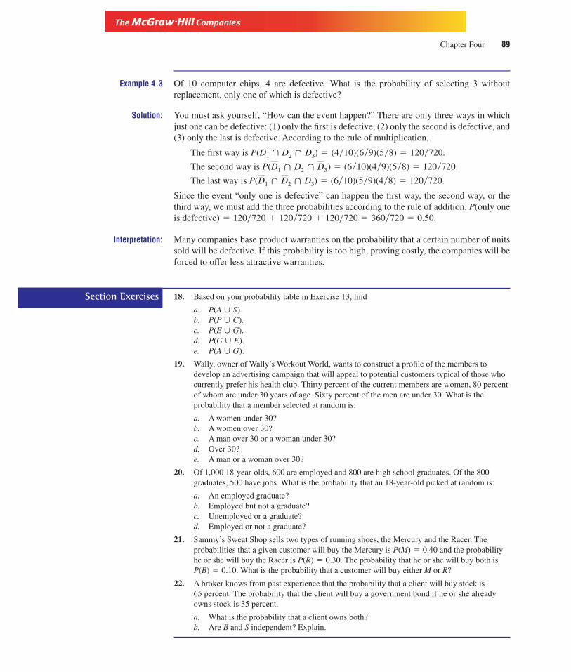
Version, Third Edition
Chapter Four 89
Example 4.3 Of 10 computer chips, 4 are defective. What is the probability of selecting 3 withoutreplacement, only one of which is defective?
Solution: You must ask yourself, “How can the event happen?” There are only three ways in whichjust one can be defective: (1) only the first is defective, (2) only the second is defective, and(3) only the last is defective. According to the rule of multiplication,
The first way is P(D1 � ) � (4�10)(6�9)(5�8) � 120�720.
The second way is P( ) � (6�10)(4�9)(5�8) � 120�720.
The last way is P( D3) � (6�10)(5�9)(4�8) � 120�720.
Since the event “only one is defective” can happen the first way, the second way, or thethird way, we must add the three probabilities according to the rule of addition. P(only oneis defective) � 120�720 � 120�720 � 120�720 � 360�720 � 0.50.
Interpretation: Many companies base product warranties on the probability that a certain number of unitssold will be defective. If this probability is too high, proving costly, the companies will beforced to offer less attractive warranties.
18. Based on your probability table in Exercise 13, find
a. P(A � S).b. P(P � C).c. P(E � G).d. P(G � E).e. P(A � G).
19. Wally, owner of Wally’s Workout World, wants to construct a profile of the members todevelop an advertising campaign that will appeal to potential customers typical of those whocurrently prefer his health club. Thirty percent of the current members are women, 80 percentof whom are under 30 years of age. Sixty percent of the men are under 30. What is theprobability that a member selected at random is:
a. A women under 30?b. A women over 30?c. A man over 30 or a woman under 30?d. Over 30?e. A man or a woman over 30?
20. Of 1,000 18-year-olds, 600 are employed and 800 are high school graduates. Of the 800graduates, 500 have jobs. What is the probability that an 18-year-old picked at random is:
a. An employed graduate?b. Employed but not a graduate?c. Unemployed or a graduate?d. Employed or not a graduate?
21. Sammy’s Sweat Shop sells two types of running shoes, the Mercury and the Racer. Theprobabilities that a given customer will buy the Mercury is P(M) � 0.40 and the probabilityhe or she will buy the Racer is P(R) � 0.30. The probability that he or she will buy both isP(B) � 0.10. What is the probability that a customer will buy either M or R?
22. A broker knows from past experience that the probability that a client will buy stock is65 percent. The probability that the client will buy a government bond if he or she alreadyowns stock is 35 percent.
a. What is the probability that a client owns both?b. Are B and S independent? Explain.
D1 � D2 �
D1 � D2 � D3
D2 � D3
Section Exercises

Version, Third Edition
90 Principles of Probability
Figure 4.2Tree Diagramfor DunhamManufacturing
P(DA) = 0.98
Not defective unit from A
Not defective unit from B
Defective unit from A
Defective unit from B
P(DA) = 0.02P(A) = 0.60
Machine A
Machine BP(B) = 0.40P(DB) = 0.96
P(DB) = 0.04
P(A � D) = P(A) � P(D A) = (0.60)(0.98)= 0.588
P(A � D) = P(A) � P(D A) = (0.60)(0.02)= 0.012
P(B � D) = P(B) � P(D B) = (0.40)(0.04)= 0.016
P(B � D) = P(B) � P(D B) = (0.40)(0.96)= 0.384
4.8 Bayes’ TheoremReverend Thomas Bayes (1702–1761) developed a concept useful in calculating certainprobabilities. Assume that Dunham Manufacturing uses two machines to produce its out-put. Machine A produces 60 percent of the total output, and machine B produces the re-maining 40 percent. Two percent of the units produced by A are defective, while B has adefect rate of 4 percent.
This is shown in the accompanying tree diagram in Figure 4.2. Assume a unit of out-put is selected at random. The first set of “branches” in the tree, indicating which machineproduced the unit, shows that the probability it came from machine A is P(A) � 0.60 andthat the probability it came from machine B is P(B) � 40. The second set of branches in-dicating quality of the unit tells us that if it came from machine A it can be either defectiveor not defective. These conditional probabilities show that the probability it is not defec-tive given it came from A is P( }A) � 0.98 and the probability it is defective given it camefrom A is P(D}A) � 0.02. The conditional probabilities for B reveal that the probability itis not defective given it came from B is P( } B) � 0.96 and the probability it is defectiveon the condition that it came from B is P(D }B) � 0.04.
D
D
Finally, we see that there are four possible outcomes to the experiment of selecting aunit of output. The probability of each is calculated by multiplying the probabilities oneach of the branches leading to it. To illustrate, the first possible outcome is that unit camefrom A and is not defective, P(A � ). Using the rule of multiplication, P(A � ) �P(A) � P( } A) � (0.60)(0.98) � 0.588. The probabilities of the three remaining out-comes can be determined similarly.
We can see directly Figure 4.2 that P(A) � 0.60. Suppose that we are told the unit isdefective and we now want to know the probability the unit came from machine A. Withthis additional information, we can revise the probability the unit was produced by ma-chine A. We now want to determine P(A }D), not just P(A).
Recall the rule of conditional probability:
However, P(D) is not readily discernible. This is where Bayes’ Theorem comes in. Thereare two ways the unit may be defective. It can come from machine A and be defective, orit can come from machine B and be defective. Using the rule of addition,
P(A}D) �P(A � D)
P(D)�
P(A) � P(D}A)P(D)
DDD

Version, Third Edition
Chapter Four 91
When we make the substitution in the denominator of the conditional probability formulaabove for P(D), Bayes’ Theorem tells us
Bayes’ Theorem [4.8]
We can now find P(A }D) as
While P(A) � 0.60, the P(A}D) � 0.429. Notice that P(A}D) � P(A) because machine Aproduces a smaller percentage of defects than does machine B.
Example 4.4 Bayes’ TheoremThe personnel department for a large firm has found that only 60 percent of the job appli-cants it interviews are actually qualified (Q) to hold a position in the company. A review ofthe firm’s records shows that of those who were qualified, 67 percent had previous statisti-cal training (T), while 20 percent of those who were not qualified had undergone earlier sta-tistical instruction. That is,
The personnel director can clearly see that given you are qualified, you are more likelyto have some statistical training than if you are not qualified (0.67 0.20). Because somuch time is wasted interviewing applicants who turn out to be unqualified, however, he isconsidering granting interviews only to those applicants who have prior training in statis-tics. He hopes to increase the probability of finding applicants qualified to fill a position.The question then becomes, Are you more likely to be qualified given that you have train-ing: P(Q/T)? If so, the personnel department could avoid delay and unnecessary cost by re-stricting interviews to those applicants with previous training in statistical analysis.
Solution: Using the rule of conditional probability
Because company records do not provide P(T), we must use Bayes’ theorem to find the de-nominator. There are two ways an applicant might have previous training: (1) the applicant
P(Q}T) �P(Q � T)
P(T)�
P(Q) � (T}Q)P(T)
�(0.60) � (.067)
P(T)
P(T}Q ) � 0.20P(T}Q) � 0.67P(Q) � 0.60
� 0.429
�(0.012)
(0.012) � (0.016)
�P(A � D)
P(A � D) � P(B � D)
P(A}D) �P(A � D)
P(D)
�P(A) � P(D}A)
P(A) � P(D}A) � P(B) � P(D}B)
P(A}D) �P(A � D)
P(A � D) � P(B � D)
� P(A) � P(D}A) � P(B) � P(D}B)
P(D) � P(A � D) � P(B � D)

Version, Third Edition
92 Principles of Probability
might be qualified and have training, P(Q � T ) and (2) the applicant might not be quali-fied and have training P(Q � T ). Thus,
Then,
While P(Q) � 0.60, P(Q }T ) � 0.834
Interpretation: To increase the probabilty of interviewing only qualified applicants, personnel should in-terview only those applicants who have previous training in statisitcal analysis.
23. James Business Equipment sells a wide range of office supplies to businesses in the Midwest.The sales manager believes she has discovered a trend that could boost sales. The results of astudy seem to suggest that law firms are more inclined to place purchase orders than are otherbusiness concerns. Her data show that the probability the general business community willbuy their supplies is 20 percent, P(B) � 0.20. Among customers over the past severalmonths, 50 percent were law firms, while 60 percent of those who did not place an orderwere law firms. The manager feels that concentrating on law offices will increase theprobability that a sales call will result in a purchase. What is your conclusion?
24. A drug company testing a new hay fever remedy finds that 60 percent of all hay feversufferers enjoy relief from their symptoms within four weeks whether or not they takemedication. Of those who obtain relief, 40 percent have taken medication, while 30 percent ofthose who do not get relief have tried medication. The drug company wants to determine theadvisability of taking medication by comparing the probability of getting relief from hayfever symptoms if sufferers do take medication to the probability of relief if sufferers do nottake medication.
4.9 Counting TechniquesMany business decisions require that we count the number of subsets we can obtain from aset. From a sales line consisting of 10 products, how many subsets of 3 products can be of-fered to customers? Seven sales personnel are in a contest to see who wins a free trip toCancun. How many different orders of finish are there? How many different phone num-bers can be assigned to a large office given the digits 0–9? Many other examples abound.We will examine four counting techniques used to answer these and many similar ques-tions: combinations, permutations, multiple choice, and multiplication.
In selecting the elements in the subsets, the distinction between permutations and com-binations depends on whether the order of the selections makes a difference. If a differentorder is a sufficient to constitute another subset, we are dealing with permutations. If twosubsets are considered the same because they have merely rearranged the same elements,combinations are involved.
� (0.834)
P(Q}T) �(0.60)(0.67)
0.482
� 0.482
� (0.60)(0.67) � (0.40)(0.20)� P(Q) � P(T}Q) � P(Q) � P(T}Q)
P(T ) � P(Q � T) � P(Q � T)
Section Exercises

Version, Third Edition
Chapter Four 93
From the first five letters of the alphabet, A, B, C, D and E, how many different sub-sets can we get? Two possibilities are: {A, B, C} and {A, C, B}. Both have the sameelements and differ only in the order in which the elements were selected. If the two sub-sets are considered different subsets because the order is different, they are seen as permu-tations. If the two subsets are seen as identical and constitute the same subset because bothhave the same elements regardless of order, they are called combinations. Simply put, withpermutations order makes a difference.
Given a set of n elements, the number of permutations, each of size r, is determined as
The number of permuta-tions of n elements [4.9]taken r at a time
where n! is read as “n factorial” and means the product of all numbers 1 through n. Thus,4! � 1 � 2 � 3 � 4 � 24. By definition 0! � 1.
The number of combinations of n elements taken r at a time is
The number of combina-tions of n elements [4.10]taken r at a time
Above, we asked, given 10 products, how many subsets of 3 products could we pack-age together and offer our customers? If we feel that the order in which we offer the 3 prod-ucts will not influence customers, that is, order will not make a difference, we must find thenumber of combinations of 10 elements taken 3 at a time.
There are 120 packages of 3 items we could offer our customers.Combinations also can be used to calculate the probability that one of the three com-
puter chips from Example 4.3 is defective. Instead of determining the probability of everyway that one is defective, we merely find the probability of one of the ways a single chip isdefective: P(D1 � ) � 120�720. Then count the number of ways one of the threeis defective as 3C1 � 3, and multiply: (3)(120�720) � 0.50.
Example 4.5 A recent court case in Madison County, Kentucky, centered on the hiring practices of thelocal telephone company. The company planned to hire 3 new employees. There were 8 ap-plicants for the jobs, 6 of whom were men. All 3 of those hired were men. A charge of sexdiscrimination was levied against the company. How would you decide?
Solution: The decision rests largely on the probability that all 3 hired are men if each applicant isgiven equal consideration without preference to gender. We must therefore determine theprobability that all three are men.
P(all three are men) �Number of ways all 3 can be men
Total number of possible outcomes
D2 � D3
� 120
10C3 �10!
3! (10 � 3!)
nCr �n!
r! (n�r)!
n Pr �n!
(n�r)!

Version, Third Edition
94 Principles of Probability
The number of ways 3 of the 6 men and none of the 2 women can be hired is
6C3 � 2C0 � 20 � 1 � 20. The total number of ways 3 out of all 8 applicants can be hiredis 8C3 � 56. Thus,
Interpretation: There is a 36% probability that all 3 employees hired are men if no preference is given togender. This event could take place roughly one out of every three times. The court ruledthat any event that could occur this frequently is not unusual and does not constitute evi-dence beyond any reasonable doubt. The charge of discrimination was not upheld.
Returning to our problem of determining how many ways we could package 3 of our10 products, if our research suggested that the order in which we packaged the 3 productswould affect sales, we should determine the number of permutations of 10 elements taken3 at a time.
Given values for n and r, since you can get another permutation just by chang-ing the order.
The number of finishing orders of the seven sales personnel vying for the trip to Can-cun noted above is 7P7 � 5,040. There are 5,040 different ways in which those seven peo-ple can be ranked or ordered according to their sales records. If the sales manager is to re-ward three members of the sales force with a trip and the order of finish is importantbecause each got a different percentage of the trip paid for, we find 7P3 � 210. On the otherhand, if all three were to win the same trip and order wouldn’t make a difference, we wouldhave 7C3 � 35.
Neither permutations nor combinations permit an element to be selected more thanonce. If duplication is allowed, the multiple-choice method of counting is used. The num-ber of multiple-choice arrangements of n elements taken r at a time is nMr � nr.
The question above concerning the number of phone lines in a large office requires themultiple-choice approach, since each of the 10 digits can be used more than once. If the of-fice uses only one extension followed by four digits, such as 555-XXXX, the number ofphone lines is 10M4 � 104 � 10,000. If a second extension is used, such as 556-XXXX,(10M4)(2), or 20,000 lines are possible.
In all of the above cases, selection was made from only one set. The phone numberscame from only one set of 10 elements. If we are to choose one element from two or moresets, the multiplication process is appropriate. This principle requires that we simply mul-tiply the number of elements in each set. George intends to buy a new automobile for hisvacation to Piney Flats. He can chose from three colors, two engine sizes, and four differ-ent interior designs. How many different modes of transport are available to George? Ac-cording to the multiplication principle, since the three sets contain three elements, two el-ements, and four elements, respectively, George must make a choice from 3 � 2 � 4 � 24different ways of reaching his destination.
nCrnPr
� 720
10P3 �10!
(10 � 3!)
P(all three are men) �20
56� 36%

Version, Third Edition
Chapter Four 95
25. From the 15 members on the board of directors of a large corporation, how many 5-membercommittees can be selected if order is not important?
26. Of 10 executives, 3 are to be selected to serve as a president, vice-president, and treasurer.How many different selections are possible?
27. Your two sick roommates send you to the student center to bring back dinner for each ofthem. If you may choose from five selections, in how many ways can you feed yourcompanions? (Hint: Does order make a difference? Can you duplicate?)
28. As a construction engineer for Base Electronics, you must determine how many differentcompact disk (CD) players you can assemble composed of a speaker system, a disk track, anda tuning mechanism if you can choose from among three different speaker systems, fourtracks, and two tuning mechanisms.
29. Of the 12 employees at Worldwide Travel Services, 7 have had special training. If 5employees are to be sent to Europe, what is the probability that 3 will be among those withthe special training?
Solved Problems1. Basic Probabilities Ortez Exports, based in Brazil, ships frozen meat products to customers
in North America (N), Europe (E) and Asia (A). The protective packages are either deluxe (D)or standard (S). The probability table below shows the relative frequencies of many of themost recent shipments.
Europe North America Asia Total
Deluxe 0.083 0.167 0.167 0.417Standard 0.167 0.167 0.250 0.584Total 0.250 0.334 0.417 1.000
To finalize several pending business decisions, Mr. Ortez must determine the likelihood ofshipping to the three destinations with either of the two package options.
a. Deluxe to Europe � P(D � E) � 0.083, as seen in the first cell showing the joint proba-bility of the two events deluxe and Europe.
b. Is Mr. Ortez more likely to ship a D to E or an S to A? P(S � A) � 0.25 0.083.c. Standard or either package to North America:
d. P(N � D) � P(N ) � P(D) � P(N � D) � 0.334 � 0.417 � 0.167 � 0.584.
2. Using Bayes’ Theorem Only 60 percent of the students in Professor Harmond’s statisticsclass pass the first test. Of those who pass, 80 percent studied; 20 percent of those who didn’tpass studied. Should you study for his tests?
This can be determined by calculating the probability that you would pass, given that youstudied. From the information above: P(P) � 0.60, P(S }P) � 0.80, and P(S } ) � 0.20.Then
P(P}S) �P(P � S)
P(S)�
P(P) � P(S}P)P(P) � P(S}P) � P(P) � P(S}P)
P
P(S � N) � P(S) � P(N) � P(S � N) � 0.584 � 0.334 � 0.167 � 0.751
Section Exercises
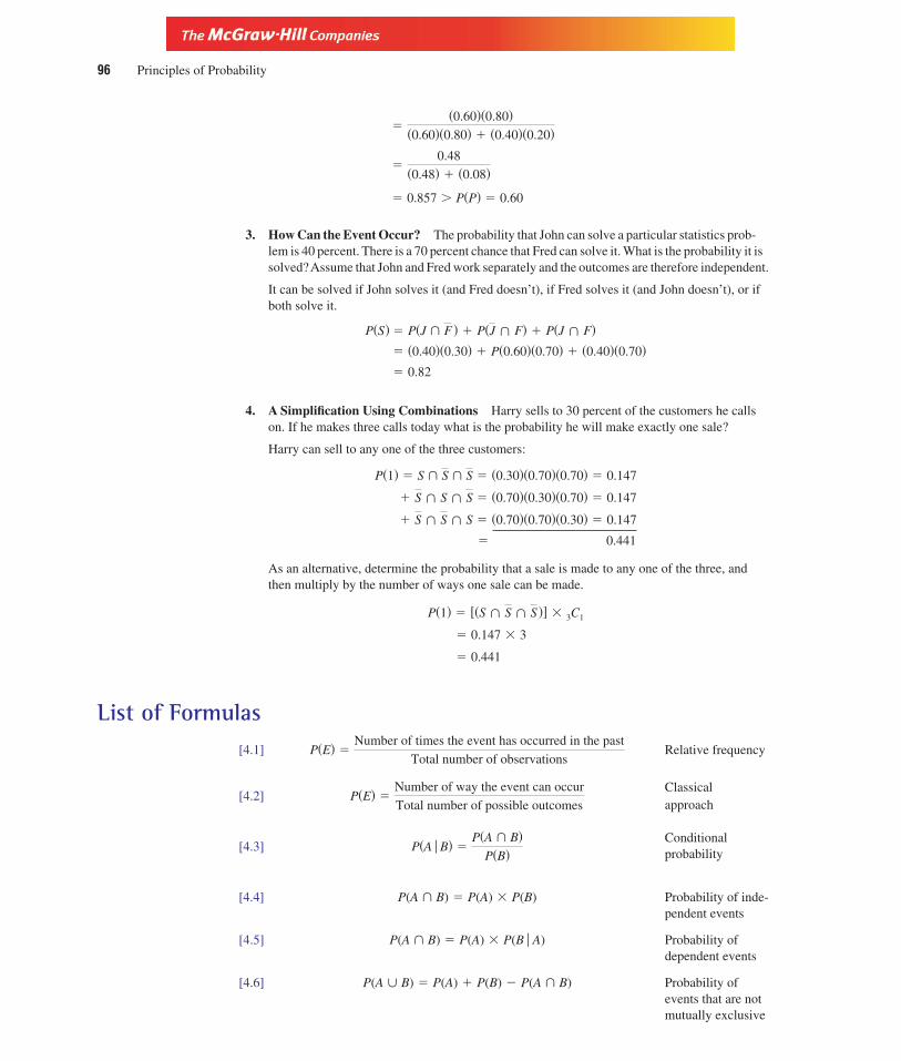
Version, Third Edition
96 Principles of Probability
3. How Can the Event Occur? The probability that John can solve a particular statistics prob-lem is 40 percent. There is a 70 percent chance that Fred can solve it. What is the probability it issolved?Assume that John and Fred work separately and the outcomes are therefore independent.
It can be solved if John solves it (and Fred doesn’t), if Fred solves it (and John doesn’t), or ifboth solve it.
4. A Simplification Using Combinations Harry sells to 30 percent of the customers he callson. If he makes three calls today what is the probability he will make exactly one sale?
Harry can sell to any one of the three customers:
� 0.441
As an alternative, determine the probability that a sale is made to any one of the three, andthen multiply by the number of ways one sale can be made.
List of Formulas[4.1] Relative frequency
[4.2]Classicalapproach
[4.3]Conditionalprobability
[4.4] P(A � B) � P(A) � P(B) Probability of inde-pendent events
[4.5] P(A � B) � P(A) � P(B }A) Probability ofdependent events
[4.6] P(A � B) � P(A) � P(B) � P(A � B) Probability ofevents that are notmutually exclusive
P(A}B) �P(A � B)
P(B)
P(E) �Number of way the event can occur
Total number of possible outcomes
P(E) �Number of times the event has occurred in the past
Total number of observations
� 0.441
� 0.147 � 3
P(1) � [(S � S � S )] � 3C1
� S � S � S � (0.70)(0.70)(0.30) � 0.147
� S � S � S � (0.70)(0.30)(0.70) � 0.147
P(1) � S � S � S � (0.30)(0.70)(0.70) � 0.147
� 0.82
� (0.40)(0.30) � P(0.60)(0.70) � (0.40)(0.70)P(S) � P(J � F ) � P(J � F) � P(J � F)
� 0.857 P(P) � 0.60
�0.48
(0.48) � (0.08)
�(0.60)(0.80)
(0.60)(0.80) � (0.40)(0.20)

Version, Third Edition
Chapter Four 97
[4.7] P(A � B) � P(A) � P(B) Probability ofmutually exclusiveevents
[4.8] Bayes’ Theorem
[4.9] Permutations
[4.10] Combinations
Chapter Exercises30. Dell Publishing has 75 different book titles classified by type and cost as follows:
Cost
Type $10 $15 $20
Fiction 10 8 3Biography 12 10 9Historical 4 17 2
Find the probability that a book selected at random is:
a. Fiction or costs $10.b. Historical and costs $20.c. Historical and costs either $10 or $15.d. Fiction and costs less than $20.e. Biographical or costs $15.f. Biographical or costs more than $10.
31. The management department at State University has access to three fax machines. Theprobability that each is out of service is 20�100, 25�100, and 30�100, respectively. Assumingindependence, find the probability that:
a. The first and the second are out of service.b. The first and the third are out of service.c. All are out of service.d. None are out of service.e. One is out of service.f. Two are out of service.g. Two or more are out of service.
32. Mark buys three different stocks. The probability the first will rise in value is 1�3, theprobability the second will rise is 3�4, and the probability the third rise is 1�10. Determine theprobability that:
a. All will rise in value.b. None will rise.c. One will rise.d. Two will rise.e. At least two will rise.f. At least one will rise.
33. A local construction company found that only 20 percent of all jobs were completed on time,while 30 percent of all jobs suffered cost overruns. In addition, cost overruns occurred75 percent of the time that a job was completed on time. The owner of the firm wants to find
nCr �n!
r! (n � r)!
nPr �n!
(n � r)!
�P(A) � P(D}A)
P(A) � P(D}A) � P(B) � P(D}B)
P(A}D) �P(A � D)
P(A � D) � P(B � D)
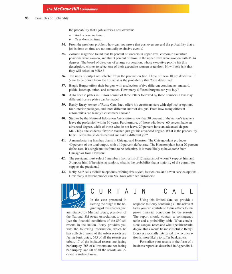
Version, Third Edition
98 Principles of Probability
C U R T A I N C A L LIn the case presented inSetting the Stage at the be-ginning of this chapter, you
are retained by Michael Berry, president ofthe National Ski Areas Association, to ana-lyze the financial conditions of the 850 skiresorts in the nation. Berry provides youwith the following information, which hehas collected: none of the urban resorts arefacing bankruptcy, 635 of all the resorts areurban, 17 of the isolated resorts are facingbankruptcy, 765 of all resorts are not facingbankruptcy, and 60 of all the resorts are lo-cated in isolated areas.
Using this limited data set, provide aresponse to Berry containing all the relevantfacts you can contribute to his efforts to im-prove financial conditions for the resorts.The report should contain a contingencytable and a probability table. What conclu-sions can you reach and what specific resultsdo you think would be most useful to Berry?Berry is especially interested in which loca-tion is more likely to suffer bankruptcy.
Formalize your results in the form of abusiness report, as described in Appendix 1.
the probability that a job suffers a cost overrun:
a. And is done on time.b. Or is done on time.
34. From the previous problem, how can you prove that cost overruns and the probability that ajob is done on time are not mutually exclusive events?
35. Fortune magazine found that 10 percent of workers in upper-level corporate executivepositions were women, and that 3 percent of those in the upper level were women with MBAdegrees. The board of directors of a large corporation, whose executive profile fits thisdescription, wishes to select one of their executive women at random. How likely is it thatthey will select an MBA?
36. Ten units of output are selected from the production line. Three of these 10 are defective. If5 are to be drawn from the 10, what is the probability that 2 are defective?
37. Biggie Burger offers their burgers with a selection of five different condiments: mustard,pickle, ketchup, onion, and tomatoes. How many different burgers can you buy?
38. Auto license plates in Illinois consist of three letters followed by three numbers. How maydifferent license plates can be made?
39. Randy Rusty, owner of Rusty Cars, Inc., offers his customers cars with eight color options,four interior packages, and three different sunroof designs. From how many differentautomobiles can Randy’s customers choose?
40. Studies by the National Education Association show that 30 percent of the nation’s teachersleave the profession within 10 years. Furthermore, of those who leave, 60 percent have anadvanced degree, while of those who do not leave, 20 percent have an advanced degree.Mr. Chips, the students’ favorite teacher, just got his advanced degree. What is the probabilityhe will leave the students behind and take a different job?
41. A manufacturing firm has plants in Chicago and Houston. The Chicago plant produces40 percent of the total output, with a 10 percent defect rate. The Houston plant has a 20 percentdefect rate. If a single unit is found to be defective, is it more likely to have come fromChicago or from Houston?
42. The president must select 5 members from a list of 12 senators, of whom 7 support him and5 oppose him. If he picks at random, what is the probability that a majority of the committeesupport the president?
43. Kelly Katz sells mobile telephones offering five styles, four colors, and seven service options.How many different phones can Ms. Katz offer her customers?

Version, Third Edition
Chapter Four 99
From the Stage to Real LifeIn the Curtain Call analysis of ski resorts, we saw that a location near a major urban areawas an important factor in their financial success. Can you think of reasons for this? Canyou think of additional factors that would contribute to the financial success of ski resorts?
The World Ski Association (www.worldski.com) is a sport membership organizationthat arranges travel packages for skiers at resorts all over the world. At this site, visit the“Directory of Benefits” and review some of the resort packages available to members.What is a common element to all of these package arrangements? Do you think that dis-count arrangements would be a factor in the success of a ski resort?
The National Ski Areas Association maintains The Official Ski Resort Guide (www.skifun.com). In the descriptions of the resorts found at this site, what features attract youto different resorts? The U.S. Collegiate Ski Association (www.beater.com/uscsa) listsscheduled ski competitions by team, date, and location. Could ski competitions influenceyour selection of a resort?

Version, Third Edition
100
C H A P T E R5Probability Distributions

Version, Third Edition
101
Chapter BlueprintThis chapter examines how probability distributions can be used to solve many common businessproblems. Both discrete and continuous variables are used in the illustrations.
Probability Distributions
Discrete distributions
Binomialdistribution
Cumulativebinomial distribution
Hypergeometricdistribution
Poissondistribution
Continuous distributions
Exponentialdistribution
Uniformdistribution
Normaldistribution
The normaldeviate
Calculatingprobabilities
Determining thevalue of X
Approximating thebinomial distribution

Version, Third Edition
102 Probability Distributions
S E T T I N G T H E S T A G EA feasibility study by professors in theCollege of Business at Bradley Univer-sity in Peoria, Illinois, revealed that on
Friday and Saturday nights the response time to 911 callsranged from 1.2 minutes to 4.6 minutes and proved to beroughly uniformly distributed. Calls were Poisson dis-tributed and arrived at the mean rate of 9 per hour. If thecity police were in response to more than 3 calls at anyone time, they could call on the assistance of the statepolice.
The mayor of the city wanted to reduce the mean re-sponse time to 2 minutes. It was estimated that the cost of more patrol cars, fire units, and personnel would be
$575,000 for every reduction of 30 seconds. The cost wasto be borne by a property tax on homes above $70,000 inassessed value. Houses in Peoria average $45,750 in valuewith a standard deviation of $15,110, and appeared to benormally distributed. At the time of the study there were42,089 houses in the city’s boundaries.
The study submitted to the mayor’s office was de-signed to evaluate the city’s response to emergencies aswell as the feasibility of achieving the mayor’s goal of re-sponse-time reduction. The final report required the appli-cation of numerous probability distributions as well as anassessment as to the potential of enacting a surcharge onproperty taxes to finance the program improvements.
Uniform Distribution
Response times
Minutes1.2 4.6
f (x) Poisson Distribution
Minutes
P(x
=x)
Normal Distribution
$45,750
Valuation
5.1 IntroductionIn the previous chapter we examined the concept of probability. Our objective was to cal-culate the probability of an event. In this chapter we continue our treatment of probabilityby examining the concepts of random variables and probability distributions. A randomvariable is a variable whose value is the result of a random event. Suppose we flip a cointhree times and note the number of heads that occur. The possible outcomes are, of course,

Version, Third Edition
0 heads, 1 head, 2 heads, or 3 heads. The random variable is the number of heads thatoccur, and the possible outcomes are the values of the random variable. As a second ex-ample, the shipping weights of containerized spring water randomly range from 10 to25 pounds. The actual weights of the containers, in pounds, are the values of the randomvariable “weight.”
As these two examples suggest, random variables may be either discrete or continu-ous. A discrete random variable may take on only certain values, often whole numbers,and results primarily from counting. The number of heads in the coin-flip experiment isan example of a discrete random variable. The values of the random variable are re-stricted to only certain numbers: 0, 1, 2, and 3. The result of the roll of a die, the num-ber of delivery trucks arriving per hour at the loading dock, and the number of library pa-trons lining up to check out their favorite books are other examples of discrete randomvariables.
A continuous random variable results primarily from measurement and can take onany value, at least within a given range. The weights of the spring water is an example be-cause the containers can take on any value between 10 and 25 pounds. Other examples ofcontinuous random variables include the heights of customers at a clothing store, the in-comes of employees at the local shopping mall and the time between the arrival of the li-brary patrons. In each case, the random variable can be measured at any value, includingfractional units. Although monetary units cannot be broken down into a continuous or infi-nite number of subdivisions (the dollar can be subdivided only 100 times), they are com-monly treated as continuous probability distributions.
A probability distribution is a display of all possible outcomes of an experimentalong with the probabilities of each outcome. From our work in Chapter 4, we can determinethat the probability of flipping a coin three times and getting (1) no heads is 1�8, (2) 1 headis 3�8, (3) 2 heads is 3�8 and (4) 3 heads is 1�8. This probability distribution is presented inTable 5.1 which shows all four outcomes and their probabilities. Notice that the probabil-ities sum to one. The same information can also be shown graphically as in Figure 5.1.
Chapter Five 103
Table 5.1Discrete ProbabilityDistribution forFlipping Heads
Outcome (heads) Probability
0 1�81 3�82 3�83 1�8
1
3/8
2/8
4/8
1/8
0 1 2 3Xi
Figure 5.1ProbabilityDistribution forFlipping Heads

Version, Third Edition
104 Probability Distributions
Probability Distribution A list of all possible outcomes of some experiment and theprobability associated with each outcome.
The probability that a random variable X can take on some specific value, xi, is writtenP(X � xi). Thus, the probability that three flips of a coin result in two heads is P(X � 2) �3�8. Note that 0 P(X � xi) 1 and �P(X � xi) � 1.
5.2 The Mean and the Variance of Discrete DistributionsJust as we calculated the mean of a data set in Chapter 3, we can also determine the meanof a probability distribution. The mean of a probability distribution is called the expectedvalue E(X), and is found by multiplying each possible outcome by its probability and sum-ming the results, as shown in Formula (5.1).
Mean or expectedvalue of a discreteprobability distribution
[5.1]
where xi are the individual outcomes
m � E(X) � �[(xi)P(xi)]
Table 5.2The DiscreteProbabilityDistribution forRolling a Die
(1) (2) (3) (4)Outcome (xi) P (xi) (xi) � P (xi) (xi � m)2 � P (xi)
1 1�6 1�6 (1 � 3.5)2 � 1�6 � 1.0422 1�6 2�6 (2 � 3.5)2 � 1�6 � 0.3753 1�6 3�6 (3 � 3.5)2 � 1�6 � 0.0424 1�6 4�6 (4 � 3.5)2 � 1�6 � 0.0425 1�6 5�6 (5 � 3.5)2 � 1�6 � 0.3756 1�6 6�6 (6 � 3.5)2 � 1�6 � 1.042
1.00 3.5 � m � E(X ) 2.92 � s2
The probability distribution for the experiment of rolling a die is shown in the first twocolumns of Table 5.2. Column (3) illustrates the calculation of the expected value for theexperiment using Formula (5.1). Each outcome is multiplied by its respective probability,and the results are summed, yielding m � E(X) � 3.5. Does this suggest that if we roll adie we can expect to get a 3.5? Hardly. It means that if we average the results of rolling adie many times (theoretically, an infinite number), we will get 3.5.
Expected Value The expected value of a discrete random variable is the weightedmean of all possible outcomes in which the weights are respective probabilities ofthose outcomes.
The variance of a probability distribution is conceptually the same as the variancewe calculated in Chapter 3. It is the mean of the squared deviations from the mean. The
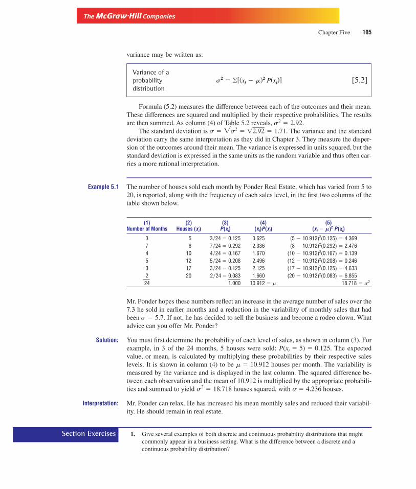
Version, Third Edition
Chapter Five 105
Section Exercises
variance may be written as:
Variance of aprobabilitydistribution
[5.2]
Formula (5.2) measures the difference between each of the outcomes and their mean.These differences are squared and multiplied by their respective probabilities. The resultsare then summed. As column (4) of Table 5.2 reveals, s2 � 2.92.
The standard deviation is The variance and the standarddeviation carry the same interpretation as they did in Chapter 3. They measure the disper-sion of the outcomes around their mean. The variance is expressed in units squared, but thestandard deviation is expressed in the same units as the random variable and thus often car-ries a more rational interpretation.
Example 5.1 The number of houses sold each month by Ponder Real Estate, which has varied from 5 to20, is reported, along with the frequency of each sales level, in the first two columns of thetable shown below.
(1) (2) (3) (4) (5)Number of Months Houses (xi) P (xi) (xi)P (xi) (xi � m)2 P (xi)
3 5 3�24 � 0.125 0.625 (5 � 10.912)2(0.125) � 4.3697 8 7�24 � 0.292 2.336 (8 � 10.912)2(0.292) � 2.4764 10 4�24 � 0.167 1.670 (10 � 10.912)2(0.167) � 0.1395 12 5�24 � 0.208 2.496 (12 � 10.912)2(0.208) � 0.2463 17 3�24 � 0.125 2.125 (17 � 10.912)2(0.125) � 4.6332 20 2�24 � 0.083 1.660 (20 � 10.912)2(0.083) � 6.855
24 1.000 10.912 � m 18.718 � s2
Mr. Ponder hopes these numbers reflect an increase in the average number of sales over the7.3 he sold in earlier months and a reduction in the variability of monthly sales that hadbeen s � 5.7. If not, he has decided to sell the business and become a rodeo clown. Whatadvice can you offer Mr. Ponder?
Solution: You must first determine the probability of each level of sales, as shown in column (3). Forexample, in 3 of the 24 months, 5 houses were sold: P(xi � 5) � 0.125. The expectedvalue, or mean, is calculated by multiplying these probabilities by their respective saleslevels. It is shown in column (4) to be � 10.912 houses per month. The variability ismeasured by the variance and is displayed in the last column. The squared difference be-tween each observation and the mean of 10.912 is multiplied by the appropriate probabili-ties and summed to yield � 2 � 18.718 houses squared, with � � 4.236 houses.
Interpretation: Mr. Ponder can relax. He has increased his mean monthly sales and reduced their variabil-ity. He should remain in real estate.
1. Give several examples of both discrete and continuous probability distributions that mightcommonly appear in a business setting. What is the difference between a discrete and acontinuous probability distribution?
s � �s2 � �2.92 � 1.71.
s2 � �[(xi � m)2 P(xi)]

Version, Third Edition
106 Probability Distributions
2. Are the following random variables discrete or continuous? In each case why did you answerthe way you did?
a. Cars sold by Honest Harry.b. The revenue Harry earns.c. Completion times for a particular job task.d. The employees required to complete that job task.
3. Calculate and interpret the expected value, the variance, and the standard deviation of theexperiment of flipping a coin three times and noting the number of heads.
4. The number of employee complaints at Fidelity Services has ranged from 0 to 6 each day, asshown in the table below. Calculate and interpret the expected value, the variance, and thestandard deviation.
Complaints Number of Days Complaints Number of Days
0 3 4 21 4 5 12 3 6 43 6
5. To gather data for a research project, a marketing major at a small university in the Midwestcounted the number of students in 50 business courses who had recently purchased CDs. Hefound no students had made such a purchase in 12 classes, 3 students had in 8 classes, 4 hadin 9 classes, 5 had in 15 classes, and 7 students in the remaining 6 classes had recently addedto their music collections. The student wanted to begin his research by summarizing his data.How can you help?
A surprisingly large number of business decisions depend on the prevailing probabil-ity distribution. One of the more important is the binomial distribution.
5.3 The Binomial Distribution—a DiscreteProbability Distribution
The experiment with the coin flip discussed above has only two possible outcomes; (1)head and (2) tail. The probability of each is known and constant from one trial (flip) to thenext and the experiment can be repeated many times. Experiments of this type follow abinomial distribution. Based on the Bernoulli process, named for Jacob Bernoulli(1654–1705), a member of a family of Swiss mathematicians, a binomial distributionexhibits four properties:
1. There must be only two possible outcomes. One is identified as a success, the otheras a failure. However, you are warned not to attach any connotation of “good” or“bad” to these terms. They are quite objective, and a “success” does not necessarilyimply a desirable outcome.
2. The probability of a success, p, remains constant from one trial to the next, as doesthe probability of a failure, 1 � p.
3. The probability of a success in one trial is totally independent of any other trial.
4. The experiment can be repeated many times.
It should be apparent why the coin flip fits the requirements for a binomial distribution.

Version, Third Edition
Chapter Five 107
Many business-related examples can also be cited. Labor unions often want to knowhow many workers (1) are interested in joining a union, as opposed to those who (2) are notinterested. Bankers may survey economic experts as to whether they feel interest rates(1) will go up or (2) will not go up. Marketing personnel want to know if a person (1) doesor (2) does not prefer a certain product. The application of the binomial distribution to busi-ness settings is almost unlimited.
A Binomial Distribution Each trial in a binomial distribution results in one of onlytwo mutually exclusive outcomes, one of which is identified as a success and the otheras a failure. The probability of each outcome remains constant from one trial to thenext.
If we know the probability that any given trial will result in a success, it is possible toestimate how many successes there will be in a given number of trials. For example, if theprobability that any single worker is interested in joining a union is known, then the prob-ability that any given number of workers in the labor force would be interested in joiningcan be estimated. The probability that out of n number of workers, a given number x wouldbe interested in joining is
The binomialformula
[5.3]
Although the formula looks rather formidable, do not despair. Probabilities for dif-ferent values of p, x, and n have been calculated for you and tabulated in Appendix III,Table B, in the back of the book.
Consider the following situation. A credit manager for American Express has foundthat p � 10 percent of the company’s card users do not pay the full amount of indebted-ness during any given month. She wants to determine the probability that of n � 20 ac-counts randomly selected, x � 5 of them are not paid. This can be written as P(X � 5}n �20, p � 0.10), which is read as “the probability of five successes given that there are 20 tri-als and the probability of a success of any one trial is 10 percent.”
The probability that 5 accounts out of the 20 sampled remain unpaid can be calculatedby using Formula (5.3). Where n � 20, X � 5, and p � 0.10, we have
If the probability that any one account is not paid in full is p � 0.10, then there is a3.19 percent chance that exactly 5 of 20 accounts selected at random will retain a positivebalance.
This information is more readily attained by using Table B. Notice that the first twocolumns in the table show possible values for n and x. Locate the value of 20 for n sincethere are 20 trials (accounts) in our experiment. Since the credit manager seeks the proba-bility x � 5 successes (unpaid accounts), locate the row containing probability values forx � 5. Proceed across that row until you find the column headed by p � 0.10. There youwill find the value 0.0319, the answer to the credit manager’s question.
20C5(0.10)5(0.90)20�5 � (15504)(0.00001)(0.2058911) � 0.0319
� nCx(p)x(1 � p)n�x
P(x) �n!
x! (n � x)!px(1 � p)n�x

Version, Third Edition
108 Probability Distributions
Consider another example of binomial distribution. Sales personnel for Widgets, Inc.,make a sale to 15 percent of the customers on whom they call. If a member of the sales staffcalls on 15 customers today, what is the probability he or she will sell exactly two widgets?Given � � 0.15, n � 15, and x � 2, locate the value for n � 15, then the row pertainingto x � 2. In that row headed by the column p � 0.15, you will find P(x � 2 } n � 15,p � 0.15) � 0.2856. There is a 28.56 percent chance that exactly two sales will be madeout of 15 sales calls.
Example 5.2 According to the Journal of Higher Education, 40 percent of all high school graduateswork during the summer to earn money for college tuition for the upcoming fall term. If7 graduates are selected at random, what is the probability that (a) 5 have summer jobs,(b) none work, (c) all work?
Solution: a. Locate the value for n � 7 and p � 0.40. The row corresponding to x � 5 yields avalue of .0774. There is a 7.74 percent probability that 5 of the 7 graduates have takensummer jobs to earn tuition money.
b. Given n � 7 and p � 0.40, the probability that none work is shown in the table to beP(x � 0) � 0.0280.
c. The probability that all students work is seen to be P(x � 7 } n � 7, p � 0.4) � 0.0016.
Interpretation: It is highly unlikely that none of the students work.
The binomial table includes values of p only up to 0.5. What do we do if the proba-bility of a success is higher? Presume that 70 percent of all the residents of Flatbush havehome computers hooked to the Internet. What is the probability that out of 10 residentschosen at random, 6 are “plugged in”? Since p 0.5, we can’t use Table B (Appendix III)without some adjustment. However, if the probability of a success (a resident is hooked tothe Internet) is P(S) � 0.70, the probability he or she is not hooked up is P(S�) � 0.30. Fur-ther, if 6 of the 10 residents are Internet users, then 4 are not. That is, 6 successes atp � 0.70 is the same as 4 failures at p � 0.30. Instead of finding x successes at p, we findn � x failures at 1.00 � p.
This practice can be illustrated by constructing two ordered arrays like those seen here,one from 0 to 10 at p � 0.70 and one from 10 to 0 at p � 0.30.
0 1 2 3 4 5 6 7 8 9 10 (p � 0.70)10 9 8 7 6 5 4 3 2 1 0 (p � 0.30)
This more clearly reveals that P(X � 6 } n � 10, p � 0.70) � P(X � 4 } n � 10,p � 0.30). From Table B (Appendix III), this is seen to be 0.2001.
A. The Mean and the Variance of a Binomial DistributionEarlier we saw how to determine the mean and the variance of a discrete distribution usingFormulas (5.1) and (5.2). However, if there are only two possible outcomes, as with a bi-nomial distribution, the mean and variance can more readily be determined as
Mean of abinomial [5.4]distribution
E(X) � m � np

Version, Third Edition
Chapter Five 109
and
Variance ofa binomial [5.5]distribution
For the Flatbush residents, if n � 10, E(X) � (10)(0.70) � 7. Out of 10 people selected atrandom, we would expect 7 to be on the Internet. The variance is s2 �(10)(0.70)(0.30) � 2.1 and the standard deviation is s � 1.45.
B. Cumulative Binomial DistributionsGiven the data in Example 5.2 for the students’ summer jobs, suppose that we wanted todetermine the probability that 3 or fewer students worked. This problem involves a cumu-lative binomial distribution since we are interested in a range of values (0 to 3) rather thana single, specific number. The ordered array below illustrates this point. The probability ofevent A (0 to 3 work) is P(A) � P(X 3).
Event A
0 1 2 3 4 5 6 7 (p � 0.40)
In Table B (Appendix III), this can be found by summing up P(X � 0) � P(X � 1) �P(X � 2) � P(X � 3) � 0.7102. For convenience, these summations are compiled inTable C, which shows the probability of the number of successes being equal to or less thansome amount. In our present case, we have P(X 3 }n � 7, p � 0.40) � 0.7102.
Remember, Table C provides the probability that the number of successes is equal toor less than some amount. Suppose we want to know P(A) � P(X � 5). Table C will notdirectly yield the probability a number of successes is equal to or greater than someamount. Take a look at the ordered array.
Event A
0 1 2 3 4 5 6 7 (p � 0.40)
Event A�
If event A is P(X � 5), then not is 4 or less, which can be found in Table C. We know thatP(A) � 1 � P( ). Then, P(X � 5}n � 7, p � 0.40) � 1 � P(X 4}n � 7, p � 0.40).From Table C, we see this is 1 � 0.9037 � 0.0963. The probability that at least 5 of the 7students have summer jobs is 9.63 percent.
Suppose we needed to determine the probability that between 3 and 5 students, inclu-sive, worked. Again, the array proves useful.
Event A
0 1 2 3 4 5 6 7 (p � 0.40)
P (X 2) � 0.4199
P (X 5) � 0.9812
P (3 X 5) � P(X 5) � P(X 2) � 0.9812 � 0.4199 � 0.5613
AA
s2 � np(1 � p)
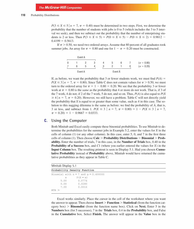
Version, Third Edition
110 Probability Distributions
P(3 X 5 } n � 7, p � 0.40) must be determined in two steps. First, we determine theprobability that the number of students with jobs is 0 to 5 (which includes the 3 to 5 inter-val we seek), and then we subtract out the probability that the number of enterprising stu-dents is 2 or less. Then P(3 X 5) � P(0 X 5) � P(0 X 2) � 0.9812 �0.4199 � 0.5613.
If p 0.50, we need two ordered arrays. Assume that 80 percent of all graduates tooksummer jobs. An array for p � 0.80 and one for 1 � p � 0.20 must be constructed.
Event A
0 1 2 3 4 5 6 7 (p � 0.80)7 6 5 4 3 2 1 0 (p � 0.20)
Event A Event A�
If, as before, we want the probability that 3 or fewer students work, we must find P(A) �P(X 3}n � 7, p � 0.80). Since Table C does not contain values for p 0.50, we mustturn to the ordered array for p � 1 � 0.80 � 0.20. We see that the probability 3 or fewerwork at p � 0.80 is the same as the probability that 4 or more do not work. That is, if 3 ofthe 7 work, 4 do not; if 2 of the 7 work, 5 do not, and so on. Thus, P(A) is also equal to P(X� 4 } n � 7, p � 0.20). However, we still have a problem. Table C will not directly yieldthe probability that X is equal to or greater than some value, such as 4 in this case. The so-lution to this nagging dilemma is the same as before: we find the probability of , that is,3 or less, and subtract from 1. P(X 3 } n � 7, p � 0.80) � 1 � P(X 3 } n � 7,p � 0.20) � 1 � 0.9667 � 0.0333.
C. Using the ComputerBoth Minitab and Excel easily compute these binomial probabilities. To use Minitab to de-termine the probabilities for the summer jobs in Example 5.2, enter the values for X in thecells of column (1) (or any other column). In this case, enter 5, 0, and 7 in the first threecells of column (1). Then choose Calc Probability Distributions Binomial Prob-ability. Enter the number of trials, 7 in this case, in the Number of Trials box, 0.40 in theProbability of a Success box, and C1 (where you earlier entered the values for X) in theInput Column box. The resulting printout is seen in Display 5.1. Had you chosen Cumu-lative Probability instead of Probability above, Minitab would have returned the cumu-lative probabilities as they appear in Table C.
Minitab Display 5.1Probability Density Function
Binomial with n � 7 and p � 0.400000x P(X � x)
5.00 0.07740.00 0.02807.00 0.0016
MTB
Excel works similarly. Place the cursor in the cell of the worksheet where you wantthe answer to appear. Then choose Insert Function Statistical (from the function cat-egory box) Binomdist (from the function name box). Click on Next. Enter 5 in theNumbers box (for 5 successes), 7 in the Trials box, 0.4 in the Probability box, and Falsein the Cumulative box. Select Finish. The answer will appear in the Value box in the
A

Version, Third Edition
Chapter Five 111
upper right corner and in the cell you designated in the worksheet. If you had entered Truein the Cumulative box, the cumulative probability for 5 successes would be reported asthey appear in Table C.
6. What are the four characteristics of a binomial distribution? Give at least three business-related examples.
7. Ten percent of the computer disks produced by a new process are defective. If there 20 disksin a box;
a. How many would you expect to be defective?b. What is the probability that the number of defective disks equals the expected number
you determined in your answer to part a?
8. From the problem above, what variation would you expect to find in defective disks from onebox to another?
9. Only 20 percent of the civilian employees at a restricted military base carry their personalidentification. If 10 employees arrive, what is the probability that the security guard willfind:
a. 8 employees with identification?b. 4 employees with identification?c. At least 4 employees with identification?d. At most 5 employees with identification?e. Between 4 and 7 employees with identification?
10. Answer the above question if 60 percent of all employees carry identification.
11. You have hired eight telephone receptionists to take telephone orders for a sporting goods lineyour company is marketing. A receptionist is busy cataloguing an order 30 percent of thetime. You do not want the probability that a customer’s call is met with a busy signal toexceed 50 percent. Should you have hired more receptionists if three customers call?
12. A student must get at least 60 percent on a true-false test with 18 questions to pass. If thestudent flips a coin to determine the answer to each question, what is the probability thestudent will pass?
5.4 The Hypergeometric DistributionAs we just learned, the binomial distribution is appropriate only if the probability of a suc-cess remains constant for each trial. This will occur if the sampling is done with replace-ment or from an infinite (or very large) population. However, if the population is rathersmall and sampling occurs without replacement, the probability of a success will vary. Ifthe probability of a success is not constant, the hypergeometric distribution is particu-larly useful. The probability function for the hypergeometric distribution is
Hypergeometricdistribution
[5.6]
where N is the population sizer is the number in the population identified as a successn is the sample sizex is the number in the sample identified as a success
P(x) � rCx N�rCn�x
NCn
Section Exercises

Version, Third Edition
112 Probability Distributions
The Hypergeometric Distribution If a sample is selected without replacement froma known finite population and contains a relatively large proportion of the population,such that the probability of a success is measurably altered from one selection to thenext, the hypergeometric distribution should be used.
Assume a racing stable has N � 10 horses, and r � 4 of them have a contagious dis-ease. What is the probability of selecting a sample of n � 3 in which there are x � 2 dis-eased horses?
There is a 30 percent probability of selecting three racehorses, two of which are ill.
Example 5.3 Use of the Hypergeometric Distribution to Examine DiscriminationIn a recent case in Johnson District Court in Kansas City, three women brought suit againsta local utility company, charging sex discrimination. Of nine people who were eligible forpromotion, four were women. Three of the nine were actually given promotions; only oneof those promoted was a woman. The other three eligible women sued the utility. A majorconsideration in the case hinged on what the probability was that out of the three peoplepromoted, no more than one woman would be chosen by chance. That is, if gender was nota factor, what is the probability that no more than one of the three promotions would go toa woman?
Solution: An economic consultant specializing in legal matters was called in by the defense attorneyto address the charges. The economist calculated the probability that, in the absence of dis-crimination, only one of the women would be promoted. This calculation was based on
N � 9; the number of people eligible for promotion
r � 4; the number in the population identified as successes (women)
n � 3; the number in the sample (those chosen for promotion)
x 1; the number of successes (women) in the sample
The probability that no more than one woman was promoted is P(X � 0) � P(X � 1).
Thus, P(X 1) � 0.4762 � 0.1190 � 0.5962.
Interpretation: There was almost a 60 percent probability that without any consideration given to gender,no more than one woman would be promoted. On the basis of these findings, as well as
P(X � 0) � 4C0 5C3
9C3
�1 � 10
84� 0.1190
P(X � 1) � 4C1 5C2
9C3
�4 � 10
84� 0.4762
� 0.30
�6 � 6
120
P(X � 2) � 4C2 10�4C3�2
10C3

Version, Third Edition
Chapter Five 113
other evidence presented in the case, the court ruled that there was not sufficient evidenceof discrimination.
A. Using the ComputerExcel works almost like magic in solving hypergeometric distributions. Simply click onINSERT FUNCTION STATISTICAL HYPERGEOMETRIC. Then enter thevalues for x, n, r, and N. The answer will appear in the Value box.
13. As assistant manager at your commodities firm, you must hire 10 people from 30 applicants,22 of whom have college degrees. What is the probability that 5 of those you hire have adegree?
14. Of the 15 senior executives in an import-export business, 12 are to sent to Japan to study anew production process. Eight of the executives already have some training in the process.What is the probability that 5 of those sent have some knowledge of the process beforeleaving for the Far East?
15. Forty workers in your office have just been given new computers. Twenty-seven have the newMMX technology. If 10 are selected at random, what is the probability that 3 are equippedwith MMX?
16. A survey in Fortune magazine (March 17, 1997) serves as the source for this problem, whichyou are asked by your supervisor to solve. Of 10 male employees, 7 had working wives.What is the probability that at most one husband has a wife who is employed outside thehome if 3 are randomly chosen?
17. From the problem above, the survey revealed that 6 of the 10 employees made in excess of$95,000 per year. Of the 3 selected, what is the probability that all 3 make over $95,000?
5.5 The Poisson DistributionA discrete random variable that is highly useful in measuring the relative frequency of anevent over some unit of time or space is the Poisson distribution. It is often used to de-scribe the number of arrivals of customers per hour, the number of industrial accidents eachmonth, the number of defective electrical connections per mile of wiring in a city’s powersystem, or the number of machines that break down and are awaiting repair.
Poisson Distribution Developed by the French mathematician Simeon Poisson(1781–1840), the Poisson distribution measures the probability of a random eventover some interval of time or space.
Two assumptions are necessary for the application of the Poisson distribution:
1. The probability of the occurrence of the event is constant for any two intervals oftime or space.
2. The occurrence of the event in any interval is independent of the occurrence in anyother interval.
Section Exercises

Version, Third Edition
114 Probability Distributions
Given these assumptions, the Poisson probability function can be expressed as
Poisson probabilityfunction [5.7]
where x is the number of times the event occursm is the mean number of occurrences per unit of time or spacee � 2.71828, the base of the natural logarithm system
Suppose we are interested in the probability that exactly five customers will arriveduring the next hour (or any given hour) of business. Simple observation over the past80 hours has shown that 800 customers have entered our business. Thus, m � 10 per hour.Using Formula (5.7),
Since this formula is a little awkward, probabilities for selected values are given in Table D.Go across the top of the table until you find m � 10. Go down that column to the row wherex � 5. There you will find 0.0378. There is a 3.78 percent chance that exactly five cus-tomers will enter the store during the next hour.
A local paving company obtained a contract with the county to maintain roads servic-ing a large urban center. The roads recently paved by this company revealed an average oftwo defects per mile after use for one year. If the county retains this paving company, whatis the probability of 3 defects in any given mile of road after carrying traffic for one year?
or 18.04 percent. To use Table D, find the column where m � 2 and the row where x � 3.There you will find the value 0.1804.
Presume for the moment that we wish to know the probability of 3 defects in 0.5 miles.Since the mean is given in occurrences per one mile (2 per one mile) it is necessary to ad-just m to fit the stipulation in the problem of 0.5 miles. We must determine what percentage0.5 miles is of 1 mile: 0.5�1 � 0.5. Then, the mean number of occurrences for this problemis m � (0.5)(2 occurrences) � 1. If the average is 2 per mile, it is going to be 1 per one-halfmile. Thus, P(X � 3}m � 1) � 0.0613. Take a look at Example 5.4, especially part c.
You should also realize that if the values in the problem exceed the limited ranges inTable D, it is possible to work the problem with most handheld calculators by remember-ing the rule of exponents: e�m � 1�em. Then,
� 0.0613
�
(1) � 1
2.718281 �3!
�13 2.71828�1
3!
P(X � 3}m � 1) �mxe�m
x!
P(3) �23 � 2.71828�2
3!� 0.1804
P(5) �(10)5 � 2.71828�10
5!� 0.0378
P(x) �mxe�m
x!

Version, Third Edition
Chapter Five 115
Example 5.4 A Poisson Distribution for Prudent StudentsProfessor Bradley encourages his statistics students to “act in a prudent manner” by con-sulting the tutor if they have any questions as they prepare for the final exam. It appears thatstudents’ arrival at the tutor’s office fits a Poisson distribution, with an average of 5.2 stu-dents every 20 minutes. Professor Bradley is concerned that if too many students need thetutor’s services, a crowding problem may develop.
a. The tutor must determine the probability that four students will arrive during any 20-minute interval, which could create the crowding problem Professor Bradley fears. Ifthis probability exceeds 20 percent, a second tutor will be hired.
b. The tutor must also calculate the probability that more than four students will arriveduring any 20-minute period. If it is greater than 50 percent, the tutor’s office hourswill be extended, allowing students to spread out the times they come to see thetutor.
c. If the probability that more than seven students arrive during any 30-minute time pe-riod exceeds 50 percent, Professor Bradley himself will offer additional tutoring.
Solution: a.
b.
c. It is given that � 5.2 for every 20 minutes. The good professor’s stipulation coversa 30-minute period. We must determine what percentage 30 is of 20: 30�20 � 1.5.Then, for every 30 minutes is 5.2(1.5) � 7.8. Thus,
Interpretation: Since P(X � 4) � 0.1681 � 20 percent, a second tutor is unnecessary. P(X 4) �0.5938 50 percent; the tutor’s office hours will be extended. And P(X 7) � 0.5133 50 percent; Professor Bradley will assist in the tutoring efforts.
A. Using the ComputerPoisson probabilities can also be obtained using Minitab and Excel. Suppose we want todetermine the probability that 4 students will arrive at the tutor’s office in part a of Exam-ple 5.4. To get the Poisson probabilities with Minitab, enter 4 in column (1) of the work-sheet. Choose Calc Probability Distribution Poisson Probability. Enter 5.2 inthe Mean box and C1 in the Input Column box.
To use Excel, choose Insert Function Statistical Poisson. Click on Next.Enter 4 in the x box, 5.2 in the Mean box and False in the Cumulative box. The answerwill appear in the Value box in the upper right-hand corner.
� 0.5133
� 1 � [P(X � 0) � . . . � P(X � 7)]
P(X 7}m � 7.8) � 1 � [P(X 7)]
� 0.5938
� 1 � [0.0055 � 0.0287 � 0.0746 � 0.1293 � 0.1681]
� 1 � [P(X � 0) � P(X � 1) � P(X � 2) � P(X � 3) � P(X � 4)]
� 1 � P(X 4}m � 5.2)P(X 4}m � 5.2)P(X � 4}m � 5.2) � 0.1681

Version, Third Edition
116 Probability Distributions
X10 20 30 40 50 60 70
P(x 30)
f (x)
P(x 40)
Figure 5.2ExponentialDistribution
Section Exercises 18. Calls come in to a switchboard at the company home office at the rate of two each minute onthe average and are known to be Poisson distributed. If the operator is distracted for oneminute, what is the probability the number of unanswered calls is:
a. Zero?b. At least one?c. Between 3 and 5, inclusive?
19. What are the probabilities in Exercise 18 if the operator is distracted for 4 minutes?
20. A manufacturing process used to make authentic plastic Incan artifacts suffers a defect rate of5 per 100 units. The units are shipped to dealers in lots of 200. If the probability that morethan 3 are defective exceeds 30 percent, you plan to stock T-shirts of the Grateful Deadinstead. Which item do you add to inventory?
21. You purchase bicycle parts from a supplier in Toledo that has 3 defects per 100 parts. You arein the market for 150 parts but will not accept a probability of more than 50 percent that morethan two parts are defective. Do you buy from this supplier?
5.6 The Exponential DistributionAs we just saw, the Poisson distribution is a discrete distribution that measures the numberof occurrences over some interval of time or space. It describes, for example, the numberof customers who might arrive during some given period. The exponential distribution,on the other hand, is a continuous distribution. It measures the passage of time betweenthose occurrences. While the Poisson distribution describes arrival rates (of people, trucks,telephone calls, etc.) within some time period, the exponential distribution estimates thelapse of time between those arrivals. If the number of occurrences is Poisson distributed,the lapse of time between occurrences will be exponentially distributed.
The probability that the lapse of time is less than or equal to some amount x is
Exponentialdistribution [5.8]
where t is the time lapsee is the base of the natural logarithm system, 2.71828m is the mean rate of occurrence
The distribution of an exponential random variable is displayed in Figure 5.2. The con-tinuously declining curve shows that as lapsed time X increases, the probability decreases.
P(X x) � 1 � e�m t

Version, Third Edition
Chapter Five 117
The probability that 30 minutes will lapse between occurrences exceeds the probability that40 minutes will lapse: P(X 30) P(X 40). This is because 30 minutes must alwayslapse before 40 minutes can.
Just as we had to adjust the mean arrival rate to fit the stipulation in a Poisson distri-bution, a similar correction is necessary for exponential distribution. Here, however, it iseasier to adjust the value for time t in Formula (5.8) to fit the time frame stipulated in theproblem. Assume that the mean arrival rate of customers is m � 1.5 per hour and we wantto know the probability that no more than two hours will lapse between arrivals. Using For-mula (5.7), t is 2. Then, P(X 2) � 1 � e�(1.5)(2) � 1 � e�3. The solution can be foundwith most handheld calculators as e�3 � 1�e3 � 0.0498. You may want to use the Poissontable (Table D) much as we did in solving Poisson problems. The secret is to set x � 0 andto ignore the negative sign for m. With the value of 3 for the exponent and x � 0, Table Dreveals e3 � 0.0498. The probability that no more than two hours will lapse between thearrival of customers is 1 � 0.0498 � 0.9502. There is a 95.02 percent chance that a sec-ond customer will enter within two hours of the first if the mean rate of arrivals is 1.5 perhour.
Trucks arrive at the loading dock at the rate of m � 2 per hour. What is the probabilityno more than 30 minutes will lapse between arrivals? The mean rate of arrival is given perhour, or 60 minutes, and the problem is stated in minutes (30 of them). To avoid the “ap-ples and oranges thing” we must find what percentage the 30 minutes is of 60. Thus,t � 30�60 � 1�2. Then, P(X 30 min.) � 1 � e�(2)(1�2) � 1 � e�1. Using a calculator,or relying on Table D by setting x � 0, we have 1 � 0.3679 � 0.6321.
Example 5.5 Cross City Cab Company schedules its taxicabs to arrive at the local airport in a Poissondistribution with a mean arrival rate of 12 per hour. You have just landed at the airport andmust get into town to close a big business deal. What is the probability you will have towait no more than 5 minutes to get a cab? Your boss is a tyrant who will not tolerate fail-ure, so if the probability another cab will be along within 5 minutes is less than 50 percent,you will rent a car for the trip to the office.
Solution: Assuming the worst, that the last cab just left, you must determine P(X 5 minutes).Since m � 12 per 60 minutes, you must determine what percentages the 5 minutes is of the60: 5�60 � 1�12. Therefore, t � 1�12 and P(X 5) � 1 � e�(12)(1�12) � 1 � e�1. Witha calculator or using Table D, you determine P(X 5) � 1 � 0.3679 � 63.21%.
Interpretation: You can relax and wait for the cab. There is a 63.21 percent ( 50 percent) chance that onewill be along within 5 minutes.
While waiting for the cab, you might consider that the probability one will arrive be-tween 5 and 10 minutes is equal to P(X 10) � P(X 5). You may also want to killsome time by reviewing your algebraic rules of exponents in case the exponent for e doesnot conveniently work out to a nice respectable whole number as it did above. Recall thate�3 � and e�0.4 � e�4�10 � .
A. Using the ComputerExcel again proves its worth in calculating exponential probabilities. Merely click on In-sert Function Statistical Expondist. Entered the adjusted value for t in the x box,
1� 10�e41e3

Version, Third Edition
118 Probability Distributions
Rel
ativ
e fr
eque
ncy
a b
Figure 5.3A UniformDistribution
the mean in the Lambda box and True in the Cumulative box. Presto, the answer appearsin the Value box.
22. Planes arrive at the small airport in Puerto Vallarta, Mexico, at the rate of two per hour. It willtake one hour to repair a ramp used to disembark passengers. What is the probability that aplane will arrive while the ramp is under repair?
23. The university’s main computer goes off line three times per week. Professor Mundane mustcomplete a project this week which requires the computer. What is the probability thecomputer will be down all week?
24. In Exercise 23, what is the probability the computer will be down for any two-week period?
25. During a typical 8-hour workday, the computers used to monitor the cooling stage in theproduction of automobile tires signal that the temperature is improperly maintained 30 times.Mr. Radial, the company’s CEO, is to drop by for a 30-minute inspection of the plant. What isthe probability he will be there when the computer’s signal is activated?
26. In Exercise 25, what is the probability Mr. Radial’s visit will be uninterrupted by thecomputer’s signal?
5.7 The Uniform DistributionThe uniform probability distribution is a distribution in which the probabilities of all theoutcomes are the same. The experiment of rolling a die shown in Table 5.2 is an example.All six outcomes had a 1�6 probability of occurrence. Figure 5.3 shows a uniform distrib-ution in which all outcomes over the distribution’s entire range of possibilities from itsminimum of a to its maximum of b are equally likely.
Uniform Distribution The probabilities in a uniform distribution are the same for allpossible outcomes.
The mean, or expected value, of a uniform distribution is halfway between its two endpoints. Thus,
Mean of a uniformdistribution
[5.9]
where a and b are the lowest and highest values, respectively.
E(x) � m �a � b
2
Section Exercises

Version, Third Edition
Chapter Five 119
f (x)
14.5
1_3
m = 16 17.2 17.5
.40
Figure 5.4A UniformDistribution ofCanned Products
Suppose the contents of the 16-ounce cans of fruit produced by Del Monte range any-where from 14.5 ounces to 17.5 ounces and fit a uniform distribution. This is displayed inFigure 5.4. The mean is
and the height is
Assume that Del Monte wanted to find the probability a single can weighed between16 and 17.2 ounces. This value is provided by the area within that range as shown in Fig-ure 5.4. The probability that a single observation will fall between two values X1 and X2 is
Probability an observationfalls between two values [5.12]P(X1 X X2) �
X2 � X1
Range
Height �1
17.5 � 14.5� 1�3
m �14.5 � 17.5
2� 16 ounces
The variance is found as
Variance of a uniformprobability distribution
[5.10]
The total area under the curve, as is the case with all continuous probability distribu-tions, must equal 1, or 100 percent. Since the area is height times width, the height is
and, therefore,
[5.11]
where b � a is the width or range of the distribution.
Height �1
b � a
Height �Area
Width
s2 �(b � a)2
12

Version, Third Edition
120 Probability Distributions
23.8 m = 25 25.5 26.2
f (x)
For the Del Monte can, it becomes
Example 5.6 Dow Chemical produces inorganic lawn fertilizer for homeowners who fertilize their grassso they can mow it more often. One type of fertilizer is sold in bags with uniformly dis-tributed weight, with a mean of 25 pounds and a range of 2.4 pounds. Harry Homeownerneeds 23 pounds to fertilize his lawn, but he is hesitant to buy only one bag since they de-viate from 25 pounds over a range of 2.4 pounds. He is also curious about the probabilityof buying a bag with more than 25.5 pounds.
Solution: If the bags average 25 pounds over a range of 2.4 pounds, then one-half of that range, or1.2 pounds, must be below 25, and the other half, above 25 pounds. Therefore, the lowestweight is 25 � 1.2 � 23.8 pounds, and the highest weight is 25 � 1.2 � 26.2 pounds, asseen in the figure. The probability of selecting a single bag that contains between 25.5 and26.2 pounds is
P(25.5 � X � 26.2) �26.2 � 25.5
2.4� 0.2917
� 0.40
P(16 � X � 17.2) �17.2 � 16
17.5 � 14.5
Interpretation: Harry need not worry. The lightest bag he could buy is 23.8 pounds. He will definitely getat least the 23 pounds he needs for his lawn. In addition, the probability of selecting a bagwith more than 25.5 pounds is 29.17 percent.
A. Using the ComputerMinitab can be used effectively to determine uniform probabilities. Enter the values forwhich you want to find probabilities in Column (1). Click on Calc Probability Distrib-utions Uniform Cumulative Probability. Enter the lowest and highest values andC1 in the Input Column box.
27. It usually takes you somewhere between 1.2 and 1.7 hours to do your statistics homework.The times are uniformly distributed. How likely are you to finish in time to meet yourbuddies 1.4 hours from now?
28. Cans of Happy-Tale Dog Food average 16 ounces, with a range of 4.2 ounces.
Section Exercises

Version, Third Edition
Chapter Five 121
a. What is the smallest can in ounces you can buy for Weiner, your toy poodle? What is thelargest can you can buy for your wolfhound, Killer?
b. If you pick a can at random, what is the probability it will weigh between 15.8 and16.5 ounces?
29. Water used by Auto-Brite to wash cars averages 30 gallons per car. The least it ever takes is27 gallons, and usage is uniformly distributed. A survey shows that cars don’t get cleanunless 32 gallons of water are used for the wash. What percentage of cars leaving Auto-Briteare clean?
30. The time required to get a lane at the local bowling alley ranges from 23.5 to 40.5 minutes.Assuming a uniform distribution, if the probability that you have to wait more than30 minutes exceeds 60 percent, you plan to play golf instead. Should you put your golf bagor your bowling bag in your trunk?
31. Since you decided to play golf, given your answer to the previous question, you learn that theaverage time to play 18 holes at this course is 4.2 hours. The fastest it has ever been finishedwas by Rapid Roy Parr, who took 2.9 hours. If times are uniformly distributed, what is theprobability you will finish in time to get home to see the football game between thePittsburgh Steelers and the Denver Broncos, which starts in 4 hours?
5.8 The Normal DistributionOf all the probability distributions we will examine, none is more important than the nor-mal distribution. In Chapter 3 you were introduced to the basic nature of the normal distri-bution, its characteristic bell-shaped symmetry, and the manner in which it related to theEmpirical Rule. At this time, you should recall that the normal distribution is a continuous(not discrete) distribution. It is used to reflect the distribution of variables such as heights,weights, distances, and other measurements that are infinitely divisible. Such continuousvariables are generally the result of measurement.
Consider for a moment a case in which ToppsWear, a large clothing manufacturer,wished to study the distribution in peoples’ heights. ToppsWear recognized that the publicis ever-changing in its physical size and proportions. In the effort to produce better-fittingclothing, management felt that a thorough analysis was needed of current trends in fashionsizes. Presume that if ToppsWear were to measure the heights of all their potential cus-tomers, they would find that these heights are normally distributed around some mean—of,say, 67 inches. That is, while the heights average 67 inches, some people are of course tallerthan that, and some are shorter. This dispersion above and below the mean could be mea-sured by the standard deviation that we calculated back in Chapter 3. Assume that the stan-dard deviation in customers’ heights is found to be 2 inches.
A graph of these heights would produce the customary bell shape. Figure 5.5 showsthis graph, placing the individual observations on the horizontal axis, and the frequency
s = 2
X (inches)m = 67
f (x)
Freq
uenc
y of
obs
erva
tion
50% 50%
Figure 5.5A NormalDistribution ofHeights forToppsWear

Version, Third Edition
122 Probability Distributions
s = 2
6761 63 65 7369 71
7975
s = 2
7975 77 8581 83
I II
68.3%68.3%68.3%95.5%68.3%99.7%
s = 4
675955 63 71
III
68.3%68.3%68.3%95.5%68.3%99.7%
68.3%68.3%68.3%95.5%68.3%99.7%
Figure 5.6 The Empirical Rule
with which each of these observations occurred on the vertical axis. If the values are indeednormal (i.e., normally distributed), then the bell-shaped curve will emerge. Recall furtherthat 50 percent of the observations (heights) are above the mean and 50 percent are belowthe mean. Similarly, of all the area under the normal curve, 50 percent of it is to the rightof the mean, and 50 percent of that area is to the left of the mean. This too is shown inFigure 5.5.
A. A Comparison of Normal DistributionsThe shape and position of a normal distribution are determined by two parameters: itsmean m and standard deviation s. Figure 5.6 shows three different normal distributions ofthe sizes that ToppsWear might find in their study of fashion trends. The first (I) is the dis-tributions described above, which has a mean of m � 67 and a standard deviation ofs � 2. It is centered at 67 with one-half of the observations above 67 and one-half below.The standard deviation of 2 indicates the degree to which the individual observations arespread out above and below 67.
A second distribution (II) has a higher mean, of m � 79, but the same standard devia-tion of s � 2. It is therefore centered farther to the right directly above 79. But since it hasthe same degree of dispersion (s � 2), it takes the same shape as the first distribution.
A third distribution (III) has the same mean as the first (m � 67) and is therefore cen-tered at the same place. However, its measure of dispersion is greater as indicated by thestandard deviation of s � 4. The observations vary above and below that mean of 67 to agreater degree than do those observations in the first distribution. Distribution III is there-fore flatter and more spread out above and below the mean of 67.

Version, Third Edition
Chapter Five 123
Despite their differences, all three of these are normal distributions. They are all sym-metrical and bell-shaped. Furthermore, as normally distributed data sets, the EmpiricalRule that we first examined back in Chapter 3 applies to each distribution. The EmpiricalRule specifies that, regardless of the value of the mean or the standard deviation,
68.3 percent of all the observations lie within one standard deviation of the mean.
95.5 percent of all the observations lie within two standard deviations of the mean.
99.7 percent of all the observations lie within three standard deviations of the mean.
Figure 5.6 illustrates the Empirical Rule. Notice that for all three data sets, regardless of thevalue for m or s, 68.3 percent of all the observations are within one s of m. Compare thefirst distribution (I) to that of the third distribution (III). Since the third distribution is morehighly dispersed, it is necessary to take in a wider interval in order to encompass the sameproportion of the observations. While the first distribution encloses 68.3 percent of all theobservations within the interval 65 to 69, the third distribution can encompass this samepercentage only within the wider interval 63 to 71.
Remember that to enclose a certain percentage of all the observations within some in-terval means also to encompass that same percentage of all the area under the curve withinthat interval. Thus, while the interval 65 to 69 contains 68.3 percent of all the observationsin the first distribution, that same interval also contains 68.3 percent of all the area underthe normal curve.
B. The Normal DeviateThere can exist an infinite number of possible normal distributions, each with its ownmean and standard deviation. Since we obviously cannot examine such a large number ofpossibilities, we need to convert all these normal distributions into one standard form. Thisconversion to the standard normal distribution is done with the conversion formula (orZ-formula)
The normal deviateor Z–formula [5.13]
where Z is the normal deviate and X is some specified value for the random variable. Afterthis conversion process, the mean of the distribution is 0 and the standard deviation is 1.That is, regardless of what the mean and standard deviation are as measured in the originalunits in the distribution, after the conversion formula is applied the mean is 0 and the stan-dard deviation is 1.
Figure 5.7 illustrates use of the ToppsWear data. The top axis measures the observa-tions of height X in inches. The mean is m � 67 inches, and the standard deviation is s � 2inches. The bottom axis reflects these heights in terms of their Z-values.
Tom Typical is 67 inches tall—the mean height of all the consumers in the ToppsWearclothing market. Using Formula (5.13), the Z-value associated with a height of X � 67 is
� 0
�67 � 67
2
Z �X � m
s
Z �X � m
s

Version, Third Edition
124 Probability Distributions
X (inches)
Z-values
67
TomSteve
0 1 1.5
70
2 3– 3 – 2 – 1.5 – 1
?63
PaulaFred
Figure 5.7ConvertingCustomer Heights
This is seen on the bottom axis, or Z-axis, in Figure 5.7. After applying the conversion for-mula, we find that the mean height of 67 inches has a Z-value of 0. If we were to convertthe heights of all the consumers in the entire market, we would find that all the resultingZ-values would have a mean of zero and a standard deviation of 1.
Z, the normal deviate, is defined as “the number of standard deviations an observationlies from the mean.” Paula Petite is 63 inches tall. Her Z-value is
As Figure 5.7 shows, 63 inches is 4 inches, or 2 standard deviations, below the mean. Con-verting X � 63 inches to its Z-value yields �2.00.
Z-Value The number of standard deviations an observation is above or below themean.
Steve Stretch is 70 inches in height. Figure 5.7 reveals that converting 70 inches to aZ-value yields
Steve’s Z-value is 1.5. He is 3 inches, or 1.5 standard deviation, above the mean height of67 inches. How tall is Fred if his Z-value is �1.5?
C. Calculating Probabilities with the Normal DeviateStandardizing a normal distribution allows us to more easily determine the probability acertain event will occur. ToppsWear personnel can find the probability a single customer isbetween, say, 67 and 69 inches tall, P(67 X 69), by simply finding the area underthe normal curve between 67 and 69. That is, if they know the area, they will know theprobability.
Think of it in this sense. Presume you are shooting at a target, two-thirds of which ispainted green and one-third red. You have the same chance of hitting any point on the target
� 1.5
Z �70 � 67
2
� �2
Z �63 � 67
2

Version, Third Edition
Chapter Five 125
X (inches)
Z-value
67
0 1
69
P(67 X 69) � P(0 Z 2) � 0.3413
X (inches)
Z-value
67
0 1
69
P(X 69) � P(Z 1) � 0.1587
0.3413 0.34130.1587
(a) (b)
X (inches)
Z-value
67
0 1.65
70.3
– 1.25
64.5
P(64.5 X 70.3) � P(– 1.25 Z 1.65) � 0.8449
X (inches)
Z-value
67
0 1.15
69.3
1.75
70.5
P(69.3 X 70.5) � P(1.15 Z 1.75) � 0.0850
0.45050.3944
0.3749
0.4599 .0850
(c) (d )
Figure 5.8Areas under theNormal Curve
as you do any other point. You are not necessarily shooting at the bull’s eye, just the targetin general. The probability that you will hit green is two-thirds. Why? Because two-thirdsof its area is green. Since you know area, you know probability. The same can be said forthe area under the normal curve.
The area associated with a given Z-value can be found in Table E in Appendix III.Figure 5.8(a) illustrates this process. We want the area between 67 and 69. The Z-valuefor 69 is
Table E gives the area under the curve from the mean to some value above it or below it.This is just the area we want. In Table E, find the Z-value of 1.0. Move to the right to thenext column headed by 0.00 to get Z � 1.00. There you will find the entry 0.3413. That is,34.13 percent of the area under the curve is between 67 and 69. There is a 34.13 percentchance that a customer picked at random in between 67 and 69 inches tall.
Although Table E gives only the area from the mean to some value above it or belowit, other probabilities can be easily found. Presume ToppsWear must determine the proba-bility that a customer is taller than 69 inches. As Figure 5.8(b) shows, we have already de-termined that 34.13 percent of all the customers are between 67 and 69 inches tall. Fur-thermore, we also know that 50 percent of all the customers are above the mean of 67. Thatleaves 0.5000 � 0.3413 � 0.1587 in the area in the tail beyond Z � 1.00. There is a15.87 percent chance that a randomly chosen customer is taller than 69 inches.
� 1.00
Z �69 � 67
2
Version, Third Edition
126 Probability Distributions
Figure 5.8(c), which seeks the area between 64.5 and 70.3, requires that we calculatetwo Z-values. Since the table will give only the area from the mean to some value above itor below it, we must determine the areas (1) between 64.5 and 67 and (2) between 67 and70.3 and add them together.
A Z-value of 1.25 (we can ignore the negative sign since the curve is symmetrical and theright half is the same as the left half) yields an area of 0.3944. For the area between 67 and70.3, we find
Table E reveals that the area is 0.4505. Thus, P(64.5 X 70.3) � 0.3944 � 0.4505 �0.8449. The probability a customer is between 64.5 and 70.3 inches tall is 84.49 percent.
To determine P(69.3 X 70.5) also requires two calculations of Z, as shown inFigure 5.8(d ). We must determine the area from 67 to 70.5, which includes the area wewant and some we do not want. Then calculate the area from 67 to 69.3 and subtract itout.
A Z-value of 1.75 yields an area of 0.4599. Then,
which produces an area of 0.3749. Then P(69.3 X 70.5) � 0.4599 � 0.3749 �0.0850.
Notice that the larger the Z-value, the less area left in the tail of the distribution. Table Eshows that as Z approaches 3.99, the encompassed area is virtually the entire 50 percentabove the mean, leaving very little in the tail beyond Z � 3.99. Therefore P(Z 3.99) � 0.
Incidentally, P(X � x) � P(X x), where x is any given value. This is because thenormal distribution is a continuous distribution. There is an infinite number of possiblevalues X can take. Therefore, to include the value of x does not increase the probability theevent will occur.
Example 5.7 TelCom Satellite provides communication services to businesses in the Chicago metropol-itan area. Company officers have learned that the average satellite transmission is 150 sec-onds, with a standard deviation of 15 seconds. Times appear to be normally distributed.
To properly estimate customer demand for its services and establish a rate structurewhich will maximize corporate profits, TelCom must determine how likely some calls are
� 1.15
Z �69.3 � 67
2
� 1.75
Z �70.5 � 67
2
� 1.65
Z �70.3 � 67
2
� �1.25
Z �64.5 � 67
2

Version, Third Edition
Chapter Five 127
X (seconds)
Z
150
0– 1.67
125
0.4525
0.0475
X (seconds)
Z
150
0 0.33
155
– 0.33
145
0.12930.1293
to happen. The director of services wants you to provide estimates of the probability that acall will last:
a. Between 125 and 150 seconds.
b. Less than 125 seconds.
c. Between 145 and 155 seconds.
d. Between 160 and 165 seconds.
Solution: a.
� �1.67
Z �125 � 150
15
From Table E, a Z-value of 1.67 yields an area of 0.4525. Therefore the probabilitythat a transmission will take between 125 and 150 seconds is 45.25 percent.
b. If 45.25 percent of the area is between 125 and 150, then 0.5000 � 0.4525 � 0.0475,or 4.75 percent of all transmissions require less than 125 seconds. The probabilitythat any transmission selected at random requires 125 seconds or less is 4.75 percent.
c.
� �0.33
Z �145 � 150
15

Version, Third Edition
128 Probability Distributions
X (seconds)
Z
150
0 0.67
160
1.0
165
0.2486
0.3413 .0927
Given Z � �0.33, the area between 145 and 150 is 0.1293. Since 155 is as farabove the mean of 150 as 145 is below the mean, the area between 150 and 155 isalso 0.1293. Therefore, P(145 X 155) � 0.1293 � 0.1293 � 0.2586.
d.
� 1
Z �165 � 150
15
With Z � 1, the area is 0.3413. To find the area between 150 and 160,
for an area of 0.2486. Therefore, P(160 X 165) � 0.3413 � 0.2486 � 0.0927.
Interpretation: Based on these probabilities, it is possible for TelCom to develop a sense of the demand forits services that will aid in establishing policies regarding customers’ use of the facilities,as well as an optimal rate structure that TelCom can charge.
D. Calculating an X-Value from a Known ProbabilityIn the previous section, you were asked to calculate a probability given some value of X.That is, you were given a value X for the random variable, and you wished to find the areabetween that value and the mean. However, sometimes you may know what probabilityyou require, and must determine what value of X will yield that probability. For example,assume that the president’s economic advisors propose a welfare program to aid the disad-vantaged, which consists of a money payment to the nation’s poorest 15 percent. The ques-tion then arises as to what income level separates the lower 15 percent of the people fromthe rest. In 1996, mean disposable personal income measured in 1982 dollars was $13,812.Assume a standard deviation of $3,550. This is shown in Figure 5.9. There is some level ofincome shown as “?” which separates the lowest 15 percent from the upper 85 percent. As-sume that incomes are normally distributed.
As shown in Figure 5.9, we know the area and seek the corresponding value for X thatis shown by the question mark. In the earlier problems, we calculated a Z-value and used it
� 0.67
Z �160 � 150
15

Version, Third Edition
Chapter Five 129
Income in 1996 dollars
Z
13,812
s = 3,550
0– 1.04
?
0.50000.35000.1500
Figure 5.9Incomes of thePoorest 15 Percent
to look up an area in the table. This time we have an area, and we can use Table E to lookup the corresponding Z-value. Although we are interested in the value of 0.15, we mustlook up 0.3500 = (0.5 � 0.15), since only the area from the mean to some value above orbelow it is given in the table. We search out in the main body of Table E the area of 0.3500.The closest we can get is 0.3508, which corresponds to a Z-value of 1.04. (Extrapolationcan be used when a greater degree of accuracy is required.) Since
and a Z-value of 1.04 was found, we have
We then solve for X and get X � $10,120. Anyone with an income of $10,120 or less willreceive the government subsidy.
Notice the negative sign for the Z-value. The algebraic sign of Z was unimportant inearlier problems because we merely used the Z-value to look up an area in Table E. How-ever, such is not the case now. In this instance, the Z-value is used for further mathematicalcalculations in solving for X. Hence, its sign is of importance. The rule of thumb is, if weare working in the area to the left of the mean, the sign is always negative.
Example 5.8 Improving Urban Fire PreventionA state commission has been formed to reduce response times of local fire departments. Agroup of experts is attempting to identify those city fire departments whose response timeis either in the lowest 10 percent, or who take longer than 90 percent of all fire departmentsin the study. Those in the first group are to serve as models for the less efficient fire units inthe second group.
Data show that the mean response times for a certain class of fire departments is12.8 minutes, with a standard deviation of 3.7 minutes.
Solution: Assuming that response times are normally distributed, the accompanying figure illustratesthe problem. It must determine two response times. The first is so short that only 10 percentof all fire units arrive at the fire within that time. The second is so long that only 10 percentof all fire units take more time. The Z-formula is used to determine each X value. To ascer-tain the quicker response time, we look up 0.4000 in the main body of Table E. Althoughwe are concerned about the bottom 10 percent, we must look up 0.4000, since that is whatthe table is designed to reveal. The entry 0.3997 is the closest, yielding a Z-value of 1.28.
�1.04 �X � 13,812
3,550
Z �X � m
s

Version, Third Edition
130 Probability Distributions
Since we are seeking a value for X in the left tail, the Z-value is given the appropriate neg-ative sign.
and
The Z-value for X2 is given a positive sign since we seek a value in the right tail greaterthan the mean.
Interpretation: Only 10 percent of the fire departments in this classification responded to fire calls in lessthan 8.06 minutes. These fire units will serve as model programs for the 10 percent of firedepartments whose fire runs exceeded 17.54 minutes.
E. Normal Approximation to the Binomial DistributionThe binomial distribution, you recall, involves a series of n trials that can produce (1) asuccess or (2) a failure. The probability of a success is indicated as p. The answers canoften be found in the binomial table or by using the binomial formula, Formula (5.3). How-ever, if n is too large, it may exceed the confines of any table and the formula may be ex-cessively cumbersome. An alternative method must be devised. The solution can be foundin the use of the normal distribution to approximate the binomial distribution. This ap-proximation is considered sufficiently accurate if np � 5 and n(1 � p) � 5 and if p isclose to 0.50.
Consider a labor union in which 40 percent of the members favor a strike. If 15 mem-bers are selected at random, what is the probability that 10 support a strike? From the bi-nomial table we find
P(X � 10}n � 15, p � 0.40) � 0.0245
X2 � 17.54 minutes
1.28 �X2 � 12.8
3.7
Z2 �X2 � m
s
X1 � 8.06 minutes
�1.28 �X1 � 12.8
3.7
Z1 �X1 � m
s
12.8
s = 3.7
X1 = ? X2 = ?
0.10 0.40 0.40 0.10

Version, Third Edition
Chapter Five 131
.20
.15
.10
.02
.01
Prob
abili
ty
151413121110
9.5
9876543210
10.5
Number of members
Figure 5.10NormalApproximation ofthe Binomial
If we were unable to use the table, we could approximate the answer using the normaldistribution. We must first find the mean m and the standard deviation s of the normal dis-tribution as
In our present case, m � (15)(0.40) � 6 and .Because there is an infinite number of possible values in a normal distribution (or any
continuous distribution), the probability that the random variable is exactly equal to somespecific value such as 10 is zero. When using a continuous distribution to estimate a dis-crete random variable, a slight adjustment is therefore necessary. This adjustment, calledthe continuity correction factor, requires that we treat the probability of exactly 10 mem-bers as the interval between 9.5 members and 10.5 members. This is illustrated in Fig-ure 5.10, which shows the probabilities for each value of the random variable (number ofmembers) taken from Table B.
s � �15(0.40)(0.60) � 1.897
m � np and s � �n(p)(1 � p)
Section Exercises
The probability that exactly 10 members favor a strike is shown by the area of the rec-tangle centered at 10. Notice that the rectangle extends from 9.5 to 10.5. The normal curveis superimposed over the rectangles.
Using the normal distribution to find P(9.5 X 10.5), we have
for an area of 0.4678, and
for an area of 0.4911. Then, P(9.5 X 10.5) � 0.4911 � 0.4678 � 0.0233, which isa close approximation of the 0.0245 found in Table B.
32. General Mills packages Cheerios in 36-ounce boxes that have a standard deviation of1.9 ounces. Weights are thought to be normally distributed. If you select one box at random,what is the probability the box will weigh:
a. Less than 34.8 ounces?b. More than 34.8 ounces?
Z �10.5 � 6
1.897� 2.37
Z �9.5 � 6
1.897� 1.85

Version, Third Edition
132 Probability Distributions
c. Between 34.3 ounces and 38.9 ounces?d. Between 39.5 ounces and 41.1 ounces?
33. As a construction engineer, you purchase bags of cement averaging 50 pounds, with astandard deviation of 5.2 pounds. The doctor told you not to lift anything over 60 poundssince your mountain climbing accident. Should you pick up a bag?
34. The brakes on new Lambourginis are advertized to last an average 35,000 miles with astandard deviation of 1,114 miles. What is the probability the one you just bought will last:
a. Over 35,000 miles?b. Less than 33,900 miles?c. Less than 37,500 miles?d. Between 35,200 and 36,900 miles?
35. Cost overruns for computer upgrades at your firm have averaged $23,500, with a standarddeviation of $9,400. As executive director of the Research Division, you do not want to riskmore than a 34 percent chance that the overrun on a newly proposed upgrade will exceed$25,000. Should you implement the upgrade?
36. Wages at the commercial banks in Illinois average $22.87 per hour, with a standard deviationof $5.87. What must your hourly wage be if you want to earn:
a. More than 80 percent of all employees?b. More than 30 percent of all employees?c. Less than 20 percent of all employees?d. More than 50 percent of all employees?
37. Employees at Coopers-Price and Lybrand work an average of 55.8 hours per week, with astandard deviation of 9.8 hours. Promotions are more likely for those employees in the upper10 percent of the time they spend working. How long must you work to improve yourchances of promotion?
38. Records show that 45 percent of all automobiles produced by Ford Motor Company containparts imported from Japan. What is the probability that out of the next 200 cars, 115 containJapanese parts?
Solved Problems1. Binomial Distribution A manufacturer in California supplies you with a prototype design
for an aircraft part your business requires. This new product, which is shipped in lots ofn � 12, suffers a 40 percent defect rate.
a. If you do not want to risk more than a 10 percent chance that 5 of the 12 are defective,should you buy from this supplier?
From Table B, P(X � 5 }n � 12, p � 0.40) � 0.2270 10%. Do not buy.
b. If you do not want to face more than a 20 percent chance that more than 5 are defective,should you purchase from this supplier?
From Table C, P(X 5 }n � 12, p � 0.40) � 1 � P(X 5 }n � 12, p � 0.40) �1 � 0.6652 � 0.3348 20%. You still shouldn’t buy from this supplier.
2. Hypergeometric Distribution A sporting goods store has N � 20 ski boots in stock, r � 8of which are in your size. If you select n � 3 pairs that you like, what is the probability thatx � 1 will fit you?
� 8C1 12C2
20C3
� 0.4632
P(X � 1) � rCx N�rCn�x
NCn

Version, Third Edition
Chapter Five 133
2.2 3.3
0.4162 0.0838
3. Poisson Distribution Wire cable used to secure bridge structures has an average of 3 de-fects per 100 yards. If you require 50 yards, what is the probability there will be one defect?
Since the mean is given in terms of 100 yards, we must determine what percentage 50 yards isof 100: 50�100 � 0.50. Then, the mean number of defects per 50 yards is (3)(0.50) � 1.5.From Table D, P(X � 1 }m � 1.5) � 0.3347, or, using the formula,
4. Exponential Distribution As manager of Burger Heaven, you observe that customers enteryour establishment at the rate of 8 per hour. What is the probability that more than 15 minutespass between the arrival of 2 customers?
Although the mean rate is originally given as 8 per 60 minutes, we want to know the probabil-ity that 15 minutes will lapse. We must determine what percentage the 15 minutes is of the 60:15�60 � 0.25. Thus, t is 0.25 and �mt � �8(.25) � �2. To determine P(X 15), weshould first find P(X 15) and subtract from 1.00. If we let x � 0 and mt � 2, Table Dshows P(X 15) � 1 � e�8(0.25) � 1 � e2 � 1 � 0.1353 � 0.8647. Then, P(X 15) � 1� 0.8647 � 0.1353.
If we use Formula (5.8) instead of the table,
Then, P(X 15) � 1 � 0.8647 � 0.1353.
5. Uniform Distribution The completion times for a job task range from 10.2 minutes to18.3 minutes and are thought to be uniformly distributed. What is the probability that it willrequire between 12.7 and 14.5 minutes to perform this task?
6. Normal Distribution The U.S. Department of Agriculture has learned from a study ofcrop yields that the daily rainfall in parts of Hawaii appears to be normally distributed with amean of 2.2 inches during the rainy season. The standard deviation was determined to be0.8 inches.
a. What is the probability it will rain more than 3.3 inches on any one day during the rainyseason?
As seen in the accompanying graph, a Z-value of 1.38 yields an area of 0.4162. Thus,P(X 3.3) � 0.5000 � 0.4162 � 0.0838.
Z �X � m
s�
3.3 � 2.2
0.8� 1.38
P(X1 X X2) �(X2 � X1)
Range�
14.5 � 12.7
8.1� 0.2222
P(X 15) � 1 � e�mt � 1 � e�8(0.25) � 1 � 0.1353 � 0.8647
P(x) �mxe�m
x!�
1.51 e�1.5
1!�
1.51 1
e1.5
1!� 0.3347

Version, Third Edition
134 Probability Distributions
2.2 2.7 3.00.2389
0.3412
2.2X = ?
0.40000.10
b. Find the probability that it will rain more than 1.3 inches.
Z �X � m
s�
1.3 � 2.2
0.80� �1.13
The Z-value of �1.13 produces an area of 0.3708, and the P(X 1.3) �0.5000 � 0.3708 � 0.8708.
c. What is the probability that the rainfall will be between 2.7 and 3.0 inches?
Z2 �2.7 � 2.2
0.80� 0.63 for an area of 0.2389
Z1 �3.0 � 2.2
0.80� 1.00 for an area of 0.3412
Therefore, P(2.7 X 3.0) � 0.3412 � 0.2389 � 0.1023.
d. How much rainfall must occur to exceed 10 percent of the daily precipitation?
As seen in the graph, an area of 0.40 is associated with a Z-value of �1.28. Therefore,
X � 1.176 inches
�1.28 �X � 2.2
0.80
2.21.3
0.50000.3708

Version, Third Edition
Chapter Five 135
67.5 71.5 72.5720.2454
0.2939
7. Normal Approximation of the Binomial Distribution Forty-five percent of all the em-ployees in the management training center at Condor Magnetics have college degrees. What isthe probability that, of 150 employees selected at random, 72 have college degrees?
The mean and standard deviation are m � (n)(p) � (150)(0.45) � 67.5 and s �
. Then, P(71.5 X 72.5) is found as
List of Formulas[5.1] Mean or expected value
of a discrete distribution
[5.2] Variance of a probability distribution
[5.3] Binomial distribution
[5.4] Mean of a binomial distribution
[5.5] Variance of a binomialdistribution
[5.6]Hypergeometricdistribution
[5.7] Poisson distribution
[5.8] Exponential distribution
[5.9]Expected value for auniform distributionE(x) � m �
a � b
2
P(X x) � 1 � e�mt
P(x) �mx e�m
x!
P(x) � rCx N�rCn�x
NCn
s2 � np(1 � p)
E(X) � m � np
P(x) � nCx (p)x � (1 � p)n�x
s2 � �[(xi � m)2 P(xi)]
m � E(X) � �[(xi)P(xi)]
P(71.5 X 72.5) � 0.2939 � 0.2454 � 0.0485
Z2 �71.5 � 67.5
6.09� 0.66 for an area of 0.2454
Z1 �72.5 � 67.5
6.09� 0.82 for an area of 0.2939
�(n)(p)(1 � p) � �(150)(0.45)(0.55) � 6.09

Version, Third Edition
136 Probability Distributions
[5.10]Variance for auniform distribution
[5.11]Height of a uniform distribution
[5.12]Probability a valuefalls within a certainrange in a uniformdistribution
[5.13] Normal deviate
Chapter Exercises39. A trucking company finds that 30 percent of its shipments arrive late. If eight shipments are
scheduled, what is the probability that:
a. Three will arrive late?b. Three or more will arrive late?c. Three or less will arrive late?d. Between three and five inclusive will arrive late?
40. A survey reveals that 60 percent of households prefer a certain brand of sports gear. If 12 house-holds are surveyed, what is the probability that this sports gear will be the choice of:
a. 7 households?b. Less than 6 households?c. 10 or more households?d. More than 2 households?
41. Temps Ltd, dispatched nine temporary day workers to the Bank of America in San Francisco.Only six of them are actually qualified to do the job to which they might be assigned. The ac-counting department selects five of the nine employees at random. What is the probabilitythat:
a. All five are qualified?b. Four are qualified?c. At least three are qualified?
42. The board of directors for ABC, Inc. consists of four economists, three accountants, and fiveengineers. If a committee of seven is to be selected at random, what is the probability it willconsist of two economists, two accountants, and three engineers?
43. Airplanes arrive at Chicago’s O’Hare airport at the average rate of 5.2 per minute. Air trafficcontrollers can safely handle a maximum of seven airplanes per minute. What is the probabil-ity that airport safety is jeopardized? Arrivals are thought to be Poisson distributed.
44. Business Week reported that 80 percent of the population thinks congressional salaries are toohigh. If 15 people are chosen to form a committee to decide by majority vote whether thesesalaries should be raised, what is the probability the vote will be to not increase them?
45. Trucks arrive for loading at the rate of 9.3 per hour on the average. The dock foreman knowsthat if six or fewer trucks arrive, only one loading dock is necessary. If more than six arrive, asecond dock must be opened. Should he open a second dock?
46. A company suffering a 10 percent defect rate sells its product in lots of 15 units. It offers a$100 discount if more than three units are defective. How much discount should the companyexpect for every 50 shipments?
Z �X � m
s
P(X1 X X2) �X2 � X1
Range
Height �1
b � a
s2 �(b � a)2
12

Version, Third Edition
Chapter Five 137
47. Janet Powell is the chief accountant for a large clothing store in a major shopping mall. Shecompletes the payrolls for all 11 employees, but seven contain errors. Janet’s boss, MarthaHolt, has become displeased with Janet’s work lately and selects five payroll records to exam-ine. It is found that three contain errors. Janet defends herself by arguing that the 3 errors wereall that she made in the 11 records. Is this a good argument?
48. The mean time between failures for General Electric’s new light bulb is 10 weeks. What is theprobability that one light bulb will fail within 15 weeks?
49. Customers enter a local restaurant at the rate of 10 per hour. What is the probability that30 minutes will lapse between the arrivals of any two customers?
50. The weights contained in boxes of cereal are uniformly distributed with a mean of 35 ouncesand a range of 3.4 ounces.
a. What are the smallest and the largest weights in the boxes?b. What is the probability that a single box contains between 32 and 33 ounces?
51. Over the past 20 years Fred has driven to work in San Francisco every day. The quickest hehas made the trip is 63 minutes. The longest it has ever taken him is 110 minutes. If drivingtimes are uniformly distributed:
a. What is Fred’s average time spent in traffic?b. What is the probability he can make it within 1.5 hours?
52. Reports show that five homicides are committed each hour in our nation’s largest cities, andthat the distribution fits a Poisson distribution. If true, what is the probability that in the next30 minutes, three people will be murdered?
53. A manufacturing process produces 1.2 defects per 100 units of output, and follows a Poissondistribution. What is the probability that the next 500 units will show three defects?
54. It normally takes two weeks to train a worker to use a computerized drill press. What is theprobability a worker can be trained in 1.5 weeks?
55. In the effort to reduce costs, Wendy’s International Inc., a popular fast-food restaurant, exam-ined the tendency for its automatic processors to determine the weights of hamburger in theirquarter-pound burgers. It was found that the weights ranged from 3.2 ounces to 4.9 ounces. Auniform distribution was assumed. What percentage of the burgers are more than one-quarterof a pound?
56. Is the normal distribution a discrete or a continuous distribution? Defend your answer. If twonormally distributed data sets have the same mean but different standard deviations, how willthe range that encompasses 68.3 percent of all the observations compare from one data set tothe other? Draw the necessary figures to illustrate how the Empirical Rule can apply to bothdistributions.
57. Monthly production costs for a print shop in Toledo have averaged $410, with a standard de-viation of $87. The manager promises the shop owner to hold costs below $300 this month. Ifcosts are normally distributed, can the owner believe the manager?
58. The accounting firm of Dooit and Quick finds that the time it takes to complete an auditingprocess is approximately normally distributed, with a mean time of 17.2 days and a standarddeviation of 3.7 days. Mr. Dooit promises to start an auditing job for your firm within 20 days,but must finish the one he has just begun. How likely is it he will keep his promise?
59. Runners at a local marathon finished the course in an average time of 180.3 minutes;s � 25.7. How fast must you run to finish in the top 10 percent?
60. Electrical connectors last an average of 18.2 months, and s � 1.7. The seller agrees to replaceone if it fails within 19 months. Out of 500 units, how many must he replace on the average?
61. Barry’s sales average $500, with s � $15.2. He gets a $100 commission only if the sale ex-ceeds $530. On the average, what is his commission out of every 25 sales?

Version, Third Edition
138 Probability Distributions
C U R T A I N C A L LIn response to the mayor’srequest, as set forth in Set-ting the Stage at the begin-
ning of this chapter, the researchers had todetermine the mean response time and thevariation in those response times. They alsohad to calculate the probability that the re-sponse time would exceed (1) 1.5 minutes,(2) 2 minutes, and (3) 3 minutes.
The mayor was also interested in theprobability that the assistance of the state
police would be needed as well as the prob-ability that 10 minutes and 15 minuteswould lapse between calls. The researchersalso had to address the cost to each house-hold with assessed valuation over $70,000to achieve the goal of reducing the mean re-sponse time to 2 minutes.
Prepare the report you would submitin accord with the format set out in Appen-dix I. Address each of these points alongwith any others you feel are pertinent.
62. Daily production at the local plant averages 7,300 tons, with s � 125 tons. On the average,out of 100 days how many times will output exceed 7,000 tons?
63. Daily receipts at one of the attractions at Dollywood in Tennessee average $1,012 with astandard deviation of $312. What is the probability that today the attraction will take in morethan $1,100?
64. Students taking the Graduate Management Aptitude Test averaged 812 with a standard devia-tion of 145. Only those in the top 20 percent can apply for a particular scholarship. GusGenius received a 900 on the test. Can he apply?
65. Storage units at Stor-N-Loc average 82.3 square feet, with s � 53.7 square feet. How manysquare feet must a unit have to be larger than 90 percent of all units?
66. According to National Geographic, 32 percent of the Australians living in the outback drink“tinnies,” a form of local beer. Out of 500 Aussies selected at random, what’s the probabilitythat at least 150 have been known to quaff a tinnie?
67. The Chicago Tribune reported that 69 percent of Russians were worse off economically afterthe revolution. Out of 800 selected at random, what is the probability that fewer than 580 suf-fer more trying conditions?
68. The Chicago Tribune reported that 56 percent of all seven-year-olds believe that Cinderellawas a real person. What is the probability that at least 50 percent of 120 seven-year-oldsbelieve so?
From the Stage to Real lifeMedian housing values are as major in economic importance to individual consumersas they are to local governments. The median price of a single family home is a gauge tohow much house a consumer can afford to buy; that is, age of house, square footage, num-ber of bathrooms, number of bedrooms, and so on. The U.S. Department of Housingand Urban Development makes median housing values available on a national basis(www.huduser.org). At this site, click on “Publications,” then click on “Housing Marketsand Demographics.” In the next list, click on “U.S. Housing Market Conditions,” and thenon “Current Issue.” In the Historical Data section, Tables 8A and 8B provide you with pricedata for new and existing single family homes from the 1960s to the present. Note the mostcurrent median price of each type.

Version, Third Edition
Chapter Five 139
The National Association of Realtors provides a selection of listings of homes for saleacross the nation (www.realtorads.com). Think of three areas of the country where youmight wish to live. At the Realtors site, for each of your desired three areas, use the nationalmedian housing prices to see listings of available houses. Are the houses desirable to you?Would you prefer something less or more expensive? Are there major differences amongthe three areas in the “amount of house” you can purchase at the median prices?
Note, that mortgage rates determine in part the price of a house you can afford. TheMortgage Loan Directory (www.mortgageloan.com) provides a selection of current mort-gage rates by state.

Version, Third Edition
140
C H A P T E R6Sampling Distributions

Version, Third Edition
141
Sampling Distributions
For sample means
Sampling error
The mean of thesample means
The standard error
Applications to anormal distribution
The Central LimitTheorem
Finite populationcorrection factor
For sample proportions
Sampling error
The standard error
Applications to anormal distribution
The Central LimitTheorem
Finite populationcorrection factor
Sampling procedures
Errors and bias
Methods ofsampling
Simple randomsampling
Systematicsampling
Stratifiedsampling
Clustersampling
Chapter BlueprintThis chapter offers an introduction to the all-important concept of sampling and the manner in whichsamples are used to draw inferences about the population.

Version, Third Edition
6.1 IntroductionPopulations are usually too large to study in their entirety. It is necessary to select a repre-sentative sample of a more manageable size. This sample is then used to draw conclusionsabout the population. For instance, we may calculate the sample mean, the statistic anduse it as an estimate of the population mean m. The statistic is used as an estimator of theparameter. By relying on a sample to draw some conclusion, or inference, about the popu-lation, we are engaging in inferential statistics.
Inferential Statistics Inferential statistics involves the use of a statistic to form aconclusion, or inference, about the corresponding parameter.
The inferential process is extremely important in many statistical analyses. In Chapters 7and 8 dealing with estimation and hypothesis testing, inferential statistics proves essential.
X,
142 Sampling Distributions
S E T T I N G T H E S T A G ESeveral wealthy clientshave chosen you as theirinvestment analyst to eval-
uate three vastly different industries. Theirintention is to identify which industry theyshould invest in. Currently, they are consid-ering the sports and leisure industry, whichseems to enjoy prosperity during recession-ary periods as people seek relief from theireconomic misfortunes. The clients antici-pate a downturn in the economy during thenext several years and therefore feel thatfunds invested in this area could producesignificant returns.
Due to the aging of the population andthe increased need for medical care, thehealth care industry is a second area of in-terest to your clients. The threat to our na-tion’s social security system and the failureto institute a national health care plan havealso stimulated the clients’ interest in thisarea as a potential investment opportunity.By investing in this field, the clients hope tocapitalize on a persistent demographic trendand, at the same time, mitigate a growingthreat to the welfare of our nation’s agingpopulation.
Finally, they want an evaluation of alarge group of firms that concentrate on envi-ronmental protection and preservation of our
nation’s wetlands. They feel that not onlycould such an investment generate financialrewards, but also they would be providing asignificant contribution to posterity for manygenerations well into the future.
Your analysis will require the applica-tion of much of the information presented inthis chapter on sampling distributions andthe probability for successful investmentportfolios for these important clients.

Version, Third Edition
Chapter Six 143
However, the value of the statistic depends on the sample taken. From any given pop-ulation of size N, it is possible to get many different samples of size n. Each sample maywell have a different mean. In fact, it is possible to get an entire distribution of different ’sfrom the various possible samples.
6.2 Sampling DistributionsIn a study of the firms on the Fortune 500 list of the nation’s largest businesses, we mightwant to take a sample of, say, n � 50. From this sample we could calculate the mean rateof return for these 50 firms. This sample mean would then serve as an estimate of m, thepopulation mean rate of return for all 500 firms.
From this list of 500 firms, it would be possible to get many different samples of size50. Specifically, we could get 500C50 different samples of size n � 50. Since 500C50 is arather large number, let us assume instead, for the sake of simplicity in our discussion, thatwe have a population of N � 4 incomes for four college students. These incomes are $100,$200, $300, and $400. The mean income can be calculated as m � $250. However, to makematters even simpler, we may feel that calculating the mean of four observations requirestoo much effort. As an alternative, we decide to select a sample of n � 2 observationsin order to estimate the “unknown” m. We would then randomly select one sample fromthe 4C2 � 6 possible samples. These six different samples and their means are shown inTable 6.1.
X
X
Table 6.1All Possible Samplesof Size n � 2 froma Population ofN � 4 Incomes
Sample Elements Sample MeansSample Xi
1 100,200 1502 100,300 2003 100,400 2504 200,300 2505 200,400 3006 300,400 350
X
With the exception of the third and fourth samples, each sample has a different mean.Assuming each sample is equally likely to be chosen, the probability of selecting a samplethat yields an equal to the population mean of 250 is only 2�6 � 33.3%. Four of the sixsamples will result in some error in the estimation process. This sampling error is the dif-ference between m and the sample mean we use to estimate it, .
Sampling Error The difference between the population parameter and the samplestatistic used to estimate the parameter.
Due just to the luck of the draw, we may select a sample of n � 2 consisting of $100and $300. The resulting mean of � $200 produces a sampling error of $250 � $200 �$50. Of course, we can never really calculate the size of the sampling error since the pop-ulation mean remains unknown. However, we must be aware that some sampling error islikely to occur.
X
(X � m)
X

Version, Third Edition
144 Sampling Distributions
Table 6.2SamplingDistribution forSamples of Sizen � 2 from aPopulation ofN � 4 Incomes
Sample Mean Number of ProbabilitySamples Yielding P
150 1 1�6200 1 1�6250 2 2�6300 1 1�6350 1 1�6
1
(X )XX
With a population of only N � 4, we can list every possible sample mean shown inTable 6.1, along with its respective probability. Such a listing is called a sampling distrib-ution, and is shown in Table 6.2 and as a histogram in Figure 6.1.
Sampling Distribution A list of all possible values for a statistic and the probabilityassociated with each value.
A. The Mean of the Sample MeansNotice that the sampling distribution of sample means is merely a list of all possible sam-ple means. These sample means, like any list of numbers, have a mean called the “mean ofthe sample means” or the grand mean. This mean of the means is calculated in the usualfashion: the individual observations (sample means) are summed and the result is dividedby the number of observations (samples). Using (pronounced X-double bar) as the sym-bol for the grand mean,
The mean of thesample means [6.1]
where K is the number of samples in the sampling distribution. Since there are 6 samplesin the present sampling distribution, we have
Notice further that the mean of the sampling distribution is equal to the mean of theoriginal population m � 250. This is no coincidence! The mean of the sampling distribution
X5
X5
�150 � 200 � 250 � 250 � 300 � 350
6� 250
X5
��X
K
X5
1/6
150
_X
_P(X )
200 250 300 350
2/6
Figure 6.1SamplingDistribution forSamples of Sizen � 2 from aPopulation ofN � 4 Incomes
Version, Third Edition
Chapter Six 145
will always equal the mean of the population Do not confuse n, the number ofobservations in a single sample, with K, the number of samples in the sampling distribu-tion. From the population of N � 4 in our present case, samples of size n � 2 yielded 4C2
� K � 6 different samples in the sampling distribution.
B. The Variance and the Standard Error of theSampling DistributionThe distribution of the sample means also has a variance. This variance in the samplemeans is like any other variance. It measures the dispersion of the individual observations(sample means) around their mean (the grand mean). Furthermore, this variance is calcu-lated like any other variance. It is the mean of the squared deviations from the mean. It isfound by
1. Determining the amount by which each of the observations (sample means) differsfrom their mean (the grand mean).
2. Squaring those deviations.
3. Averaging the squared deviations by dividing by the number of sample means, K.
Thus, where is the variance of the sampling distribution of sample means, we find
Variance of the sampling distributionof sample means
[6.2]
Given the six sample means above,
If we were to take the square root of the variance in the distribution of these samplemeans, we would have the standard error of the sampling distribution, . Thus,
Standard error of thesampling distributionof sample means
[6.3]
In our present case
The standard error of the sampling distribution (or standard error) is a measure of thedispersion of the sample means around m. It is analogous to the standard deviation we cal-culated in Chapter 3, which measured the dispersion of individual observations around theirmean. Since the difference between and m is the sampling error, any measure of the ten-dency for the sample mean to deviate from m is rightfully called the standard error. Thus, thestandard error measures the tendency to suffer sampling error in our effort to estimate m.sx
X
� 64.55 dollars
sx � �4,167
sx � �s2x
sx
� 4,167 dollars squared
s2x �
�(X � X5)2
K�
�(X � m)2
K
s2x
(X5
� m).
s2x �
(150 � 250)2 � (200 � 250)2 � (250 � 250)2 � (250 � 250)2 � (300 � 250)2 � (350 � 250)2
6

Version, Third Edition
146 Sampling Distributions
Example 6.1 Sales for East Coast Manufacturing (ECM) over the past five months in thousands of dol-lars have been 68, 73, 65, 80, and 72. Assuming these five months constitute the popula-tion, the mean is clearly m � 71.6. As marketing director for ECM, you wish to estimatethis “unknown” m by taking a sample of size n � 3. You hope that the sampling error youwill likely suffer is relatively small. Create the sampling distribution and comment on thelikely sampling error.
Solution: There are 5C3 � 10 samples in the sampling distribution:
Sample SampleSample Elements Sample Mean Sample Elements Sample MeanNumber Xi Number Xi
1 68,73,65 68.67 6 68,80,72 73.332 68,73,80 73.67 7 73,65,80 72.673 68,73,72 71.00 8 73,65,72 70.004 68,65,80 71.00 9 73,80,72 75.005 68,65,72 68.33 10 65,80,72 72.33
The sampling distribution is: P( )
68.67 1�1073.67 1�1071.00 2�1068.33 1�1073.33 1�1072.67 1�1070.00 1�1075.00 1�1072.33 1�10
The mean of the sampling distribution is
The variance and the standard error of the sampling distribution are
Interpretation: The mean of the sampling distribution equals the mean of the original population m �71.6. No surprise there. The standard error, which measures the degree of dispersion of the10 sample means around m, thus indicates how far the sample mean may vary from thepopulation mean. Is this what you had in mind when you hoped for a “relatively small”sampling error?
sx � �s2x � �4.31 � 2.08 thousand dollars
� 4.31 thousand dollars squared
�(68.68 � 71.6)2 � (73.67 � 71.6)2 � ≥ � (72.33 � 71.6)2
10
s2x �
�(X � m)2
K
X5
�68.67 � 73.67 � 71.00 � 71.00 �≥� 72.33
10� 71.6 � m
XX
XX

Version, Third Edition
Chapter Six 147
As you may have noticed by now, Formula (6.2) requires a lot of third-grade arith-metic to calculate the variance of the sampling distribution. A close approximation can beobtained by
and [6.4]
This, of course, requires the assumption that the population variance s2 is known.Formula (6.4) is appropriate only if sampling is done with replacement, or if the sam-
ple is taken from a very large (virtually infinite) population. If sampling is done without re-placement and if the sample size is more than 5 percent of the population, n 0.05N, thefinite population correction factor (fpc) must be applied. The proper formula for thestandard error then becomes
Standard error using the fpc [6.5]
where is the fpc.
If n is small relative to N (less than 5 percent), the fpc approaches 1 and is thereforeunnecessary since multiplying by 1 does not change the value of the standard error.
C. The Impact of Sample Size on the Standard ErrorGiven a population of size N � 1000, do you think you would get a more accurate estimateof the population mean m with a sample of size n � 100 or a larger sample of size n � 900?Unquestionably, a more exact estimate is likely with a larger sample. This presumption isverified by examining Formula (6. ). It can be seen that as n increases, will decrease.The fact that larger samples lead to smaller sampling errors will become increasingly im-portant as we progress in our study of inferential statistics.
1. Define the following terms in your own language. Give examples of each.
a. Sampling distribution.b. Mean of the means.c. Variance and standard error of the sampling distribution.
2. A population of weekly factory outputs in thousands of tons is 200, 250, 150, 200, and 300.Develop a sampling distribution and calculate the mean of the means and the standard error forsamples of size n � 2.
s x
�
N � n
N � 1
s x �s
� n
�
N � n
N � 1
s x �s
� n
s
2x �
s
2
n
Section Exercises
4

Version, Third Edition
148 Sampling Distributions
3. What will happen to the standard error in the preceding exercise if n � 3? Why is there adifference?
4. Samples of n � 40 are taken from a large population with a mean of 100 and standarddeviation of 25. Calculate and interpret the standard error.
5. Repeat the preceding exercise with n � 100. Discuss the difference.
6.3 The Central Limit TheoremFrom our discussion thus far, it should be evident that it is possible to take many samplesof some given size from any population. These samples give rise to an entire distributionof sample means. If the original population is normally distributed, the distribution of sam-ple means will also be normally distributed. That is, all the sample means will themselvesgraph as a normal distribution.
This is seen in Figure 6.2. The top graph shows the distribution of the individual ob-servations Xi in the population to be normally distributed centered at a mean m � 500 witha standard deviation s � 50. Notice that the individual observations Xi are measured onthe horizontal axis.
X (sample means)X = m = 500=
–
m = 500Xi (individual observations)
The distributionof the population
The distributionof the sample means
s = 50
sx = = = 10s
n5025
Figure 6.2A Distribution of Sample Meansfrom a NormalPopulation
The bottom graph of Figure 6.2 reflects the distribution of the sample means that willresult if all samples of size n � 25 are taken. Notice that the sample means are measuredon the horizontal axis. These sample means are also normally distributed and centered atthe population mean since � m � 500. That is, the mean of the sample means equals themean of the population. Notice further that the dispersion of the original populations � 50 is greater than the dispersion of the sample means � 10.The Xi are more spread out than the since .
The question might arise as to what the distribution of sample means looks like if theoriginal population is not normally distributed. The answer is provided by the CentralLimit Theorem. The central limit theorem states that for any population, as n gets larger,the distribution of sample means approaches a normal distribution with a mean � m
and a standard error sx � s��n.X5
sx � s��nXs
sx � s��n � 50��25
X5
Xs

Version, Third Edition
Chapter Six 149
XX = m = 1000=
–
X–
m = 1000Xi
The distributionof the population
The distributionof the sample means(n = 50)
s = 100
sx = = = 14.14s
n100 50
X = m = 1000=
The distributionof the sample means(n = 100)
sx = = = 10s
n100 100
ModeMedian
Mean
Figure 6.3A Distribution ofSample Means froma NonnormalPopulation
Central Limit Theorem As n gets larger, the distribution of sample means will ap-proach a normal distribution with a mean and a standard error
Thus, even if the population is not normally distributed, the sampling distribution ofsample means will be normal if n is large enough. The standard rule of thumb is that if n isat least 30, the central limit theorem will ensure a normal distribution in the sample meanseven if the population is not normal.
Take a look at Figure 6.3. Assume that the population in the top graph, which is clearlynot normally distributed, has a mean of m � 1000 with a standard deviation of s � 100.The center graph displays the distribution of the sample means that would result if samplesof size n � 50 were taken. The distribution of sample means is normally distributed andcentered at � m � 1000. Moreover, the dispersion of the sample means as measured bythe standard error is Notice that the are less dis-persed than the individual observations in the original population: s s��n.
Xssx � s��n � 100��50 � 14.14.X5
sx � s��n.X5
� m
The bottom graph of Figure 6.3 illustrates what happens to the distribution of as thesample size increases. If the sample size is increased to n � 100, the standard error be-comes The sample means are more tightly compactedaround the population mean m � 1000. Since more of the sample means are closer to thepopulation mean, the standard error suffered in the effort to estimate m is less. This is whylarger samples are likely to produce more accurate estimates of the population mean.
sx � s��n � 100��100 � 10.
Xs

Version, Third Edition
150 Sampling Distributions
6. State the Central Limit Theorem in your own words.
7. What is meant by the standard deviation of the population and the standard error of thesampling distribution of sample means? How do they relate and how do they compare in size?Draw graphs in your response.
8. What happens to the standard error as the sample size increases? Draw graphs to illustrate.
6.4 Using the Sampling DistributionThe importance of the foregoing discussion can be recognized only if we recall that manydecisions are made on the basis of sample results. A business manager may sample a prod-uct to determine whether certain production specifications are being met. A governmentofficial will take a sample of residents to decide whether a certain tax plan or welfare pro-gram will produce the desired results. Academicians often sample students to ascertain theimpact of instructional efforts.
Generally speaking, samples have a very direct and consequential impact on decisionsthat are made. Therefore, any conclusion we can draw or knowledge we have regarding asample is quite important. An extremely common and quite useful application of a sam-pling distribution is to determine the probability that a sample mean will fall within a givenrange. Given that the sampling distribution will be normally distributed because (1) thesample is taken from a normal population, or (2) n � 30 and the Central Limit Theorem en-sures normality in the sampling process, the normal deviate may be used to gain informa-tion essential to the decision-making process.
In Chapter 5 we determined the probability of selecting one observation that would fallwithin a given range. Recall from Example 5.7 that TelCom recorded telephone messagesfor its customers that averaged 150 seconds, with a standard deviation of 15 seconds.TelCom wished to determine the probability that one single call lasted between 125 and150 seconds. This was done using the conversion formula, or Z-formula,
in which X is a single observation of interest and s is the population standard deviation.However, many business decisions depend on an entire sample—not just one observa-
tion. In this case, the conversion formula must be altered to account for the fact that we areinterested not in one observation X but in the mean of several observations, Therefore,when sampling is done, the conversion formula becomes
[6.6]
The value of interest in the numerator is not a single observation Xi, but the mean ofn observations Furthermore, the denominator is not the population standard deviation s,but the standard error of the sampling distribution Instead of determining the probabilitysx.
X.
Z �X � m
sx
X.
Z �X � m
s
Section Exercises
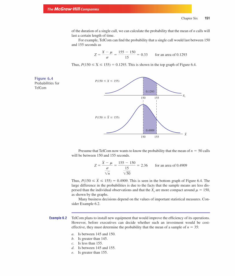
Version, Third Edition
Chapter Six 151
X150
–
–
150
155
155Xi
P(150 X 155)
P(150 X 155)
0.1293
0.4909
Figure 6.4Probabilities forTelCom
of the duration of a single call, we can calculate the probability that the mean of n calls willlast a certain length of time.
For example, TelCom can find the probability that a single call would last between 150and 155 seconds as
Thus, P(150 X 155) � 0.1293. This is shown in the top graph of Figure 6.4.
Z �X � m
s�
155 � 150
15� 0.33 for an area of 0.1293
Presume that TelCom now wants to know the probability that the mean of n � 50 callswill be between 150 and 155 seconds.
Thus, P(150 155) � 0.4909. This is seen in the bottom graph of Figure 6.4. Thelarge difference in the probabilities is due to the facts that the sample means are less dis-persed than the individual observations and that the are more compact around m � 150,as shown by the graphs.
Many business decisions depend on the values of important statistical measures. Con-sider Example 6.2.
Example 6.2 TelCom plans to install new equipment that would improve the efficiency of its operations.However, before executives can decide whether such an investment would be cost-effective, they must determine the probability that the mean of a sample of n � 35:
a. Is between 145 and 150.b. Is greater than 145.c. Is less than 155.d. Is between 145 and 155.e. Is greater than 155.
Xs
X
Z �X � m
s
�n
�155 � 150
15
�50
� 2.36 for an area of 0.4909

Version, Third Edition
152 Sampling Distributions
Solution: a. P(145 150)X
b. P(X � 145)
� 0.4756
P(145 X 150) � P(�1.97 Z 0)
Z �X � m
sx
�145 � 150
15��35� �1.97 or an area of 0.4756
_X (seconds)
150145
0.4756
0–1.97Z
0.5000
_X (seconds)
150 155
0.4756
0 1.97Z
0.5000
c. P(X 155)
� 0.9756
� 0.4756 � 0.5000
P(X � 145) � P(Z � �1.97)
Z �X � m
sx
�145 � 150
2.54� �1.97 or an area of 0.4756
150145
0.4756 _X
0– 1.97Z
Z �X � m
sx
�155 � 150
2.54� 1.97 or an area of 0.4756

Version, Third Edition
Chapter Six 153
_X (seconds)
150 155
0.4756
0 1.97Z
0.0244
_X (seconds)
150145
0.4756
0–1.97Z
0.4756
155
1.97
d. P(145 155). We must find the area between 145 and 150, and add it to thearea between 150 and 155.
X
� 0.9756
� 0.4756 � 0.5000
P(X 155) � P(Z 1.97)
e. P(X � 155)
� 0.9512
� 0.4756 � 0.4756
P(145 X 155) � P(�1.97 Z 1.97)
Z2 �X � m
sx
�155 � 150
2.54� 1.97 or an area of 0.4756
Z1 �X � m
sx
�145 � 150
2.54� �1.97 or an area of 0.4756
Interpretation: On the basis of this information, TelCom can make more intelligent decisions regarding theneed for new equipment.
� 0.0244
� 0.5000 � 0.4756
P(X � 155) � P(Z � 1.97)
Z �X � m
sx
�155 � 150
2.54� 1.97 or an area of 0.4756
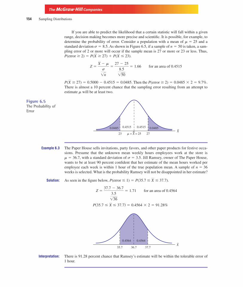
Version, Third Edition
154 Sampling Distributions
X–
2723
0.4515 0.04850.0485 0.4515
m = X = 25=
Figure 6.5The Probability ofError
If you are able to predict the likelihood that a certain statistic will fall within a givenrange, decision making becomes more precise and scientific. It is possible, for example, todetermine the probability of error. Consider a population with a mean of m � 25 and astandard deviation s � 8.5. As shown in Figure 6.5, if a sample of n � 50 is taken, a sam-pling error of 2 or more will occur if the sample mean is 27 or more or 23 or less. Thus,P(error � 2) � P( � 27) � P( 23).
P( � 27) � 0.5000 � 0.4515 � 0.0485. Then the P(error � 2) � 0.0485 � 2 � 9.7%.There is almost a 10 percent chance that the sampling error resulting from an attempt toestimate m will be at least two.
X
Z �X � m
s
�n
�27 � 25
8.5
�50
� 1.66 for an area of 0.4515
XX
Example 6.3 The Paper House sells invitations, party favors, and other paper products for festive occa-sions. Presume that the unknown mean weekly hours employees work at the store ism � 36.7, with a standard deviation of s � 3.5. Jill Ramsey, owner of The Paper House,wants to be at least 90 percent confident that her estimate of the mean hours worked peremployee each week is within 1 hour of the true population mean. A sample of n � 36weeks is selected. What is the probability Ramsey will not be disappointed in her estimate?
Solution: As seen in the figure below, P(error 1) � P(35.7 37.7).
P(35.7 X 37.7) � 0.4564 � 2 � 91.28%
Z �37.7 � 36.7
3.5
�36
� 1.71 for an area of 0.4564
X
X–
37.735.7
0.45640.4564
36.7
Interpretation: There is 91.28 percent chance that Ramsey’s estimate will be within the tolerable error of1 hour.

Version, Third Edition
Chapter Six 155
Section Exercises 9. The population of miles driven by truckers for Over the Road Van Lines exhibits a mean of8,500, with a standard deviation of 1,950. If a sample of n � 100 drivers is taken, what is theprobability the mean will:
a. Exceed 8,900?b. Be less than 8,000?c. Be between 8,200 and 8,700?d. Be between 8,100 and 8,400?
10. Cans of soda sold at Minute Mart average 16.1 ounces, with a standard deviation of 1.2 ounces.If a sample of n � 200 is taken, what is the probability that the mean will be:
a. Less than 16.27?b. At least 15.93?c. Between 15.9 and 16.3?
11. A survey by the National Education Association revealed that high school seniors watch anaverage of 37.2 hours of television per week. Assume a standard deviation of 5.4 hours. In asample of n � 500 students, how likely is it the sample mean will be:
a. More than 38 hours?b. Less than 36.6 hours?c. Between 36.4 and 37.9 hours?
12. Daily water consumption in Dry Hole, Texas, averages 18.9 gallons per household, with a stan-dard deviation of 3.6 gallons. The city commissioner wishes to estimate this unknown meanwith a sample of 100 households. How likely is it the sampling error will exceed 0.5 gallons?
6.5 The Sampling Distribution for ProportionsAlthough our discussion thus far has focused exclusively on means, many business mattersare concerned with the population proportion p.Amarketing firm may want to know whethera customer (1) buys or (2) does not buy the product. A bank must often determine whether adepositor will (1) ask or (2) not ask for a car loan. Many business firms must determine theprobability that a capital budgeting project (1) will or (2) will not generate a positive return.In these cases the sample proportion p is used to estimate the unknown parameter p.
The sampling process for proportions is much like that for means. From any popula-tion it is possible to get many different samples of some given size. Each sample will haveits own proportion of “successes,” p. However, as with means, the expected value of thesampling distribution of sample proportions will equal the proportion of successes in thepopulation: E(p) � p.
Lugget Furniture asks the entire population of all N � 4 customers whether they sawthe Lugget advertisement in this morning newspaper. A response of “yes” is recorded as asuccess, and “no” as a failure. The four customers respond Y1, N2, N3, and Y4. The popula-tion proportion of successes is p � 0.50. Samples of size n � 2 are taken, and the propor-tion of successes is recorded in Table 6.3.
The expected value (mean) of the sampling distribution of sample proportions is
The expected value of thesampling distribution [6.7]
E(p) ��p
K

Version, Third Edition
156 Sampling Distributions
and the standard error is
[6.8]
As with means, if n 0.05N, the fpc is required and the standard error becomes
[6.9]
In our present case with Lugget Furniture,
and, using the fpc
Our newly developed tools for sample proportions allow us to determine probabilitiesthat can prove very useful in making important business decisions. This is accomplished byapplying the normal deviate to the sampling distribution for proportions:
[6.10]
Example 6.4 BelLabs obtains components for its cellular telephones in lots of 200 from a firm in PaloAlto. The component has a defect rate of 10 percent. A policy recently established byBelLabs states that if the next shipment has:
Z �p � p
sp
� 0.289
� �(0.50) (1 � 0.50)2
�4 � 2
4 � 1
sp � �(p) (1 � p)n
�N � n
N � 1
E(p) ��p
K�
3
6� 0.50 � p
sp � �(p) (1 � p)n
�N � n
N � 1
sp � �(p) (1 � p)n
Table 6.3The SamplingDistribution ofProportions
Xi Number of Successes p (Proportion of successes)
Y1, N2 1 0.50Y1, N3 1 0.50Y1, Y4 2 1.00N2, N3 0 0.00N2, Y4 1 0.50N3, Y4 1 0.50
3.00

Version, Third Edition
Chapter Six 157
0.120.05
0.32890.49130.0087 0.1711
0.1
a. More than 12 percent defects, it will definitely find a new supplier.
b. Between 10 percent and 12 percent defects, it will consider a new supplier.
c. Between 5 percent and 10 percent defects, it will definitely not get a new supplier.
d. Less than 5 percent defects, it will increase their orders.
Which decision is BelLabs most likely to make?
Solution: Since the population size N is not give, it is reasonable to assume that BelLabs buys manycomponents and the sample size of n � 200 is less than 0.05 N and the fpc is therefore notneeded.
a. P(p 0.12):
sp � �(0.1) (0.9)200
� 0.021
b. From part a, P(0.10 p 0.12) � 0.3289.
c. P(0.05 p 0.10):
d. From part c, P(p � 0.05) � 0.0087.
Interpretation: Since part c has the highest probability, BelLabs will stay with its current supplier.
13. An opinion poll of 1000 residents of a large city asks whether they favor a rise in taxes to payfor a new sports stadium. If more than 85 percent support the tax, a referendum will be intro-duced in the city’s next election. If the unknown population proportion of all residents whofavor the tax is p � 0.82, 82 percent, what is the probability it will be placed on the next ballot?
14. Thirty percent of all employees have advanced training. If, in a sample of 500 employees, lessthan 27 percent are adequately prepared, all new hirees will be required to enroll in a trainingprogram. What is the probability the program will be initiated?
15. Based on a sample of 100 teachers, a study is undertaken to analyze their preference of thecurrent Teachers’ Insurance Annuity Fund-College Retirement Equity Fund (TIAA-CREF) re-tirement program available to them. If fewer than 60 percent are satisfied with TIAA-CREF,an alternative will be found. Assuming p � 65 percent, what is the probability the currentplan will be supplemented?
Z �0.05 � 0.10
0.021� �2.38 for an area of 0.4913
P(p 0.12): 0.5000 � 0.3289 � 0.1711
Z �0.12 � 0.10
0.021� 0.95 for an area of 0.3289
Section Exercises
Version, Third Edition
158 Sampling Distributions
16. The proportion of all customers at Pizza Hut who eat on-site is 75 percent. In a sample of100 patrons, what is the probability that less than 20 percent take their meal home?
17. Sixty percent of all cattle in a large herd have anthrax. Out of 100 cattle chosen at random,what is the probability that at least 50 will have to be cut from the herd?
6.6 Sampling MethodsWe have repeatedly emphasized the need to select a sample representative of the popula-tion. A sample that misrepresents the population will introduce sampling error and produceinaccurate estimates of the population parameters.
There are two basic sources of sampling error. The first is just plain bad luck. Due tothe “luck of the draw,” our sample might contain elements that are not characteristic of thepopulation. Fate may dictate that certain selections in the sample are atypically larger thanmost of those in the population, which would result in an overestimation of the parameter.Or perhaps many of the sample elements tend to be smaller than what are typically foundin the population, in which case an underestimation would result.
A second source of sampling error is sampling bias. Bias results from the tendency tofavor the selection of certain samples over others in the collection of our sample data. Aclassic example of sampling bias occurred in the 1936 presidential election. Franklin D.Roosevelt was running on the Democratic ballot against Alf Landon, the Republican can-didate. A survey of voters conducted by the Literary Digest (which long ago ceased publi-cation) revealed that Landon would win in a veritable landslide. When the smoke liftedafter the election, the editors of Literary Digest tried courageously to determine how theycould have been so wrong!
They soon discovered their blunder. In selecting the people for their sample, they tooknames from two sources: the phone book and their own subscription rolls. Remember, in1936 the nation was in the midst of the Great Depression. Most people, rightfully or wrong-fully, blamed the Republicans for this economic catastrophe and steadfastly refused to votefor anyone with that party affiliation. Literary Digest chose people who were less affectedby harsh financial conditions and could actually afford a telephone and a regular subscrip-tion to a magazine. The people used in the survey were therefore not representative of thenation as a whole. The sample tended to favor in its selection those voters who were notso adamantly opposed to the Republicans. No wonder the magazine is no longer in circu-lation.
There are many other instances in which the selection of the sample can result in error.It is therefore wise to ensure that the collection of sample data follows a prescribed methodthat has proved its ability to minimize such error. Although an exhaustive examination ofsampling methods is beyond the scope of this text, a brief look at proper sampling proce-dures is warranted at this point.
A. Simple Random SampleAs we have seen, several different samples can be selected from any population. Taking asimple random sample ensures that each sample of some given size has the same proba-bility of being selected. Assume a national fast-food chain wishes to randomly select 5 ofthe 50 states to sample consumers’ taste. A simple random sample will guarantee that the
50C5 � 2,118,760 samples of size 5 will all have the same likelihood of being used in thestudy.

Version, Third Edition
Chapter Six 159
A simple random sample can be obtained by merely listing the observations on iden-tical pieces of paper, placing them in a hat and drawing out the desired number. In addi-tion, a random numbers table may also be used. The table is often generated by a computerin which each of the 10 digits (0–9) has an equal probability of being selected. If a three-digit table is desired, the computer might randomly select 4, 2, 7, 5, 2, 6, 1, 0, 5, and so on,forming the random numbers 427, 526, and 105. A random numbers table is provided inTable A.
B. Systematic SamplingA systematic sample is formed by selecting every ith item from the population. If i is setequal to 10, a systematic sample consists of every tenth observation in the population. Thepopulation must be ordered or listed in a random fashion.
The first selection must be randomly determined, and if i � 10, it will be somewherewithin the first 10 observations. The exact starting point can be identified either by select-ing a number between 1 and 10 drawn from a hat, or by using a table of random numbers.In any event, every tenth observation thereafter is selected.
The process of systematic sampling is advantageous in that it doesn’t require a highlyskilled expert to count to 10 and record the outcome. In addition, the method permits flex-ibility in that i can be set to 10, 100, 1,000, or any other desired number. Determination ofthe proper value for i is also quite easy. If we wish to select a sample of size 100 from apopulation of 1,000, i must be 10.
The primary danger that must be avoided is the occurrence of a pattern in the orderingof the population. For example, listing the population alphabetically assumes a random dis-tribution throughout the alphabet.
C. Stratified SamplingThe U.S. Department of Agriculture recently became interested in the impact of droughtconditions on the production of wheat. Of particular concern was the rate of bankruptciescausing farmers to lose their land. It was felt that an account of the production levels byfarmers in Kansas, Oklahoma, Nebraska, and South Dakota, the four states hardest hit bythe drought, might prove useful in devising a relief program. The department decided thata sample of this year’s harvest should be taken for several hundred farmers from eachstate.
However, it was noted that the number of farmers was quite different in each state. Ifa simple random sample was taken from all four states as a whole, it might very well in-clude proportionately too few farmers from some states and too many from others. Thiswould result in a nonrepresentative sample, which would increase the sampling error.
The Department of Agriculture decided to take a stratified sample by dividing all thefarmers into subgroups or strata (hence the term stratified sampling). In this case, the logi-cal subgroups would be the four states in question. The proportion of farmers included inthe sample from each state would be set equal to those proportions of all farmers in eachstate: If Kansas farmers made up 30 percent of all the farmers in all four states, then 30 per-cent of the farmers in the sample would be randomly selected from Kansas.
A stratified sample is taken by forcing the proportions of the sample from each stratato conform to the pattern of the population. It is commonly employed when the populationis heterogeneous, or dissimilar, yet certain homogeneous subgroups can be isolated. In thismanner the researcher can increase accuracy beyond that obtained by a simple randomsample of similar size.

Version, Third Edition
160 Sampling Distributions
D. Cluster SamplingAnother alternative technique, cluster sampling, offers certain advantages over othermethods. It consists of dividing the entire population into clusters, or groups, and then se-lecting a sample of these clusters. All observations in these selected clusters are included inthe sample. To illustrate, consider the following example. The U.S. Department of Agri-culture, in its study of drought conditions, might decide that a cluster sample is preferable.A cluster sample is taken by identifying the counties in each state as clusters. A sample ofthese counties (clusters) is then chosen randomly by using a table of random numbers orsome other generally accepted means. All farmers in the counties selected in this mannerare included in the sample. This procedure is often easier and quicker than simple randomsampling or stratified sampling. For example, if it is necessary to travel to each farm in thesample to observe the effects of the drought, it is easier to visit several farmers in the samecounty.
It is also possible to combine stratified sampling with cluster sampling. In our agricul-tural example, it might be wise to select for our sample a number of counties from eachstate proportional to the total number of counties in all four states.
Certain problems can arise in the use of cluster sampling. If an abnormally large (orsmall) percentage of the farmers in a selected cluster tend to use irrigation to enhance cropyields, the sample results may be biased.
This discussion is in no way a complete account of sampling methods or the problemsthat can arise in the process of searching for a representative sample to be used to draw sta-tistical inferences. A study of sampling techniques constitutes an entire course in and of it-self and is beyond the scope of this text. However, due to the importance of the samplingprocess, even the beginning student should be aware of sampling fundamentals.
Solved Problems1. Investment records show that the mean rate of return for firms in the consumer goods industry
is 30 percent, with a standard deviation of 12 percent. If a sample of 250 such firms isselected, what is the probability that the mean of these firms will exceed 31 percent?
As the graph shows, the probability that the sample mean is between 30 percent and 31 per-cent is
Z �0.31 � 0.30
0.12
�250
� 1.32 for an area of 0.4066
0.31–X
0.4066 0.0934
0.30
Probability thatthe mean of the250 firms willexceed 31%
Thus, P( 0.31) � 0.5000 � 0.4066 � 0.0934.X

Version, Third Edition
Chapter Six 161
0.20
0.27640.2236
0.22
Probability youbuy elsewhere
2. Only 22 percent of all the firms in the consumer goods industry market their products directlyto the final consumer. If a sample of 250 firms reveals a proportion of more than 20 percentwho engage in direct marketing, you plan to make your next purchase from the firms in thisindustry. How likely are you to spend your hard-earned money elsewhere?
Z �0.20 � 0.22
�(0.22)(0.78)250
� �0.76 for an area of 0.2764
Thus, P(p .20) � 0.7765, and the probability you do not buy from these firms is1.00 � 0.7765 � 0.2236.
List of Formulas
[6.1] Mean of the sample means
[6.2]Variance of the sampling distributionof sample means
[6.3] Standard error of the samplingdistribution of sample means
[6.4] Standard error of the sampling distribution
[6.5]Standard error with finite populationcorrection factor
[6.6] Normal deviate for means
[6.7] Expected value of proportions
[6.8] Standard error of proportions
[6.9]Standard error with finite populationcorrection factor
[6.10] Normal deviate for proportionsZ �p � p
sp
sp � �(p) (1 � p)n
�N � n
N � 1
sp � �(p) (1 � p)n
E(p) ��p
K
Z �X � m
sx
sx �s
�n�N � n
N � 1
sx �s
�n
sx � �s2x
s2x �
� (X � m)2
K
X5
��X
K

Version, Third Edition
162 Sampling Distributions
Chapter Exercises18. If a sample is taken in which n � 30, what problem might we have in working with it?
19. If several samples of a given size are taken from a population, what will influence the vari-ability of those sample means? What happens to that variability as n increases?
20. From a single population, two sampling distributions are formed by taking all possible sam-ples of a given size to get sampling distribution A, and all possible samples of a different sizeto get sampling distribution B. These distributions are graphed below. Which distribution con-tains the larger sample size? How can you tell?
_ _X = m
_X
Distribution A
_ _X = m
_X
Distribution B
21. A population of weekly sales (in $1,000’s) at Blazing Salads, a vegetarian restaurant inChicago, is 27, 32, 17, 21, and 32.
a. Calculate and interpret s.b. Set n � 2 and develop the sampling distribution.c. Calculate and interpret How does it relate to s?d. Calculate and interpret m.e. Calculate and interpret How does it compare with m.
22. Using the data in Exercise 21, set n � 3 and
a. develop the sampling distribution.b. calculate and How do they differ from the values in Exercise 21, and why?
23. A sample of n � 50 is taken from a large population with a mean of 12.2 and a standard devi-ation of 4.1. What are the mean and the standard error of the sampling distribution of samplemeans?
24. Customers at the Madison Hair Garden, a beauty shop in Madison, Connecticut, average40.7 per day, with a standard deviation of 12.9. If a sample of 100 days is taken, what is theprobability that the mean number of customers will exceed 43?
25. Jim Sears manufactures farm equipment. His work requires the use of steel bars which musthave a mean length of at least 50 inches. The bars can be purchased from a supplier inKansas City whose bars average only 47 inches, with a standard deviation of 12 inches, orfrom a supplier in Dallas whose bars average 49 inches, with a standard deviation of3.6 inches. If Sears is to buy 81 bars, should he use the supplier in Kansas City or the one inDallas?
26. According to Business Week, the average years of experience of airline pilots is 25.2. As-sume a standard deviation of 12 years. This year you must make 36 business flights. Youhope the average length of experience for the pilots of your flights is over 30. How likely isit that 30?
27. The mean deposits at First of America Bank in Peoria are $7,012, with a standard deviation of$532, and they are normally distributed.
a. If one deposit is selected at random, what is the probability that it exceeds $6,911?b. If a sample of n � 35 deposits is randomly selected, what is the probability that the mean
will exceed $6,911?
X
sx.X5
X5
sx .

Version, Third Edition
Chapter Six 163
c. Why does taking a sample decrease your answer? Draw graphs, one directly above theother, to illustrate.
28. The mean production level at a local manufacturing plant is 47.3 units per day, with a stan-dard deviation of 12.7. The plant manager will take a sample of 100 days. If the samplemean exceeds 49, she promises to give all employees a Christmas bonus. How likely are theemployees to enjoy a merry Christmas?
29. Incomes for production line workers in Chicago average $21.15 per hour with a standarddeviation of $5.15. These incomes are skewed left. Describe the sampling distribution ofincomes for sample size 100. Draw the distributions for both the original population and thesampling distribution.
30. If the sample size in Exercise 29 was 64, how would the sampling distribution compare?Graph both.
31. A local mechanic charges $110 on the average to complete a certain repair. Records show astandard deviation of $21.50 in billings. A customer recently complained that his bill of$115.50 was excessive. After considerable haggling, the mechanic agreed to refund the moneyif a sample of 36 similar jobs revealed a mean billing less than the customer’s bill. Do youthink the mechanic was wise in offering this settlement?
32. A manufacturing process produces units that average 10 inches in length with a standard devi-ation of 3.2 inches. If only those units between 9.5 and 10.5 inches can be used, how manyout of a sample of 100 must be thrown away?
33. In a computer assignment given a sophomore statistics class, the students averaged14.2 errors, with a standard deviation of 4.3.
a. What is the probability that you (or any given single student) will have more than 13 errors in your assignment if errors are known to be normally distributed?
b. If errors are not known to be normally distributed, what is the probability that a sample of36 students will average more than 13 errors?
c. Why are your answers different? Draw two graphs, one directly above the other, to illus-trate.
d. Why was the assumption of normality required in part a and not in part b?
34. The standard deviation in the amount of time it takes to train a worker to perform a task is40 minutes. A random sample of 64 workers is taken.
a. What is the probability the sample mean will exceed the population mean by more than5 minutes?
b. What is the probability the sample mean is more than 8 minutes less than the populationmean?
35. A random sample of 81 purchases at a local department store was taken to estimate the meanof all purchases. It is known that the population standard deviation is $25.
a. What is the probability the sample mean will not overstate the population mean by morethan $4?
b. What is the probability the sample mean will understate the population mean by morethan $1?
36. The average retirement fund in TIAA for a population of teachers is $40,715, with a standarddeviation of $19,015. Find the probability that a sample of 75 teachers will yield a samplingerror less than $1,000.
37. National figures show that 32 percent of all students fail their first statistics test. If 100 stu-dents are selected at random, what is the probability more than 40 fail?
38. An industrial process generates 8 percent defective units. You purchase 100 units. What is theprobability that less than 10 percent are defective?
Version, Third Edition
164 Sampling Distributions
39. From the same industrial process cited in the previous exercise, you again purchase 100 units.What is the probability that less than 10 percent are defective?
40. A producer of VCRs advertises that 28 percent of the VCRs sold on the market are its brand.Of 150 recent sales, exactly 40 were produced by this company. How do you feel about thecompany’s claim?
41. Your customers require that at least 90 percent of your products are without defects. A sampleof 500 reveals 31 defects. Are you meeting customers’ specifications?
42. The maker of a new computer proves to you that you will experience only 9 percent down-time for repairs and maintenance with their new model. A check of your current hardware re-veals that out of the last 90 hours, 12 hours were downtime. Is the new computer more reli-able than your current model?
43. Five cards are laid out on a table face down. Your friend claims he has ESP. You select a cardat random without revealing your choice to your friend. Out of 200 attempts, he correctlyidentifies 54 cards. Do you believe your friend has ESP?
44. A corporation is going to float a new stock issue. Law requires that current stockholders begiven the first opportunity to buy any new issue. Management feels that 45 percent of currentstockholders will want to make a purchase. A random sample of 130 stockholders is selected,63 of whom express a desire to buy.
a. What is the standard error of the sample proportion?b. What is the mean of the sampling distribution of sample proportions?c. What is the probability of obtaining the results described in the problem if p � 0.45?
45. Sears has determined that 17 percent of all purchases made during the Christmas season arereturned. If a store sells 150 video games, what is the probability that at most 20 percent willbe returned?
46. Without working the problem, explain what would happen to the answer in the previous prob-lem if n increased to 200. Why?
C U R T A I N C A L LIn Setting the Stage at thebeginning of this chapter,you were charged with the
responsibility of analyzing three industriesto identify in which one several of your im-portant clients might invest their funds. Thethree areas in which your clients are inter-ested are sports and leisure, the health carefield, and environment protection. Presumethat the unknown mean rates of return inthese three fields are 8 percent, 23 percent,and 15 percent respectively, and that thestandard deviation in these returns are 3 per-cent, 5 percent, and 7 percent. Bankruptcyrates are 12 percent, 7.5 percent, and 3 per-cent in the three industries, respectively.
The clients are concerned most aboutthe mean rate of return their investment willyield as well as the risk of default they willhave to bear due to bankruptcy. Your analy-sis is to include your estimates of the proba-bilities of default and the potential rates ofreturn. Your clients are very cautious in-vestors and are also requesting estimates ofthe probability of any errors in your analy-sis. You plan to sample 50 firms from thesports and leisure industry, 150 firms in thehealth care industry, and 250 firms con-cerned with wildlife management. Fully ex-plain and justify any additional assumptionsyou must make to complete the analysis.Prepare your final report in accord with therules set out in Appendix I for report writing.

Version, Third Edition
From the Stage to Real LifeAs an individual investor, you are able to learn a great deal about specific companies onthe Internet. If you are considering companies you have heard tips about, a good place tobegin your information gathering is at the companies’ web sites. Marriott Hotels (www.marriott.com) is a major corporation in the leisure industry. What information does its website provide you about its consumer services? What investor information is provided at thissite? Similarly, Aetna (www.aetnaushc.com) is a major managed health care provider.What information is made available at this site for its customers? For its investors? Finally,Environment One Corporation (www.eone.com) manufactures pollution control equip-ment. What information does this company make available to its customers? Its investors?
You can look up specific corporation financial data on the Edgar database maintainedby the Securities and Exchange Commission (www.sec.gov).
Chapter Six 165

Version, Third Edition
166
C H A P T E R7Estimating withConfidence Intervals

Version, Third Edition
167
Chapter BlueprintChapter 6 showed how sampling distributions of the population mean and the population proportioncan be used to generate point estimates of m and p. This chapter shows how interval estimates can beformed for these two parameters and how levels of confidence can be assigned to these intervals.
Confidence Intervals
Principle andinterpretationof confidenceintervals
Forpopulationmeans
Forpopulationproportions
Controllinginterval width
Propertiesof goodestimators
Unbiased
Efficient
Consistent
Sufficient
Change thelevel ofconfidence
Changesamplesize
Large samples
Small samples
The a-value:the probabilityof error
Determiningsample sizes
For m
For p

Version, Third Edition
7.1 IntroductionBy now you are well aware that populations are generally too large to study in their en-tirety. Their size requires that we select samples, which we then use to draw inferencesabout the populations. If a manager of a retail store wished to know the mean expenditureby her customers last year, she would find it difficult to calculate the average of the hun-dreds or perhaps thousands of customers who shopped in her store. It would be much eas-ier to estimate the population mean with the mean of a representative sample.
There are at least two types of estimators commonly used for this purpose: a point es-timate and an interval estimate. A point estimate uses a statistic to estimate the parameterat a single value or point. The store manager may select a sample of n � 500 customersand find the mean expenditure to be $37.10. This value serves as the point estimate forthe population mean.
An interval estimate specifies a range within which the unknown parameter may fall.The manager may decide the population mean lies somewhere between $35 and $38. Suchan interval is often accompanied by a statement as to the level of confidence placed in itsaccuracy. It is therefore called a confidence interval.
X �
168 Estimating with Confidence Intervals
S E T T I N G T H E S T A G EIn 1997 the Federal Bu-reau of Investigation (FBI)implemented revolution-
ary procedures to facilitate the apprehen-sion of people wanted for serious crimes.A spokesperson from the Bureau’s CrimeStatistics Division appeared on the LarryKing Live show on Cable News Network(CNN) to discuss the procedures that wouldmake our streets safer. She cited several sta-tistics the FBI collected describing motives,techniques and frequencies of crimes thatshe felt were useful in profiling at-largecriminals the bureau desperately wanted tocapture.
Her discussion focused on the bu-reau’s efforts to maintain a large databaseon crime statistics that could be used topredict criminal activity and thus to betteranticipate where and when an unlawful actmight take place. She cited several casesthat had been solved due in large part towork by professional statisticians to pro-vide estimates of recidivism rates of of-fenders as well as other activities that couldprovide some clue that might aid in theirarrest. This information proved extremelyuseful to agents in the field whose job it isto locate those on the FBI’s Most WantedList.

Version, Third Edition
Chapter Seven 169
Estimates A point estimate uses a single number or value to pinpoint an estimate ofthe parameter. A confidence interval denotes a range within which the parametermight be found, and the level of confidence that the interval contains the parameter.
Actually there are three levels of confidence commonly associated with confidence in-tervals: 99, 95, and 90 percent. There is nothing magical about these three values. We couldcalculate an 82 percent confidence interval if we so desired. These three levels of confi-dence, called confidence coefficients, are simply conventional. The manager referred toabove might be 95 percent confident that the population mean is between $35 and $38.
Interval estimates enjoy certain advantages over point estimates. Due to samplingerror, will likely not equal m. However, we have no way of knowing how large the sam-pling error is. Intervals are therefore used to account for this unknown discrepancy.
We begin with a discussion of what a confidence interval is and how to interpret it.
A. The Principle of a Confidence IntervalA confidence interval has a lower confidence limit (LCL) and an upper confidence limit(UCL). These limits are found by first calculating the sample mean, . A certain amount isthen added to to get the UCL, and the same amount is subtracted from to get the LCL.The determination of that amount is the subject of this chapter.
How can we construct an interval and then argue that we can be 95 percent confidentthat it contains m if we don’t even know what the population mean is? Recall from our dis-cussion of the Empirical Rule that 95.5 percent of all sample means lie within two standarderrors of the population mean. Then, the population mean lies within two standard errors of95.5 percent of all sample means. Therefore, starting with any sample mean, if we movetwo standard errors above that mean and two standard errors below that mean, we can be95.5 percent confident that the resulting interval contains the unknown population mean.
Remember, our discussion of sampling distributions showed that, from any popula-tion, we can get many different samples of some given size, each with its own mean. Fig-ure 7.1 on page 170 shows six of these possible sample means. If our sample yields aninterval extending two standard errors above and two standard errors below does indeedinclude the unknown value of the population mean. Similarly, if our sample had yielded amean of the resulting interval would also include the population mean. Notice that only
and lie so far from the population mean that an interval �2 standard errors does notinclude the population mean. All other sample means will produce an interval that containsthe population mean. The key to remember, then, is this: Since the population mean lieswithin two standard errors of 95.5 percent of all these sample means, then, given any sam-ple mean, we can be 95.5 percent certain that the interval of two standard errors around thatsample mean contains the unknown population mean.
If we wish to construct the more conventional 95 percent interval (rather than the95.5 percent discussed above), how many standard errors must we move above and belowthe sample mean? As Figure 7.2 shows, because the Z-table contains values only for thearea above or below the mean, we must divide the 95 percent by 2, yielding 0.4750. We thenfind the Z-value corresponding to an area of 0.4750, which is Z � 1.96. Thus, to constructa 95 percent confidence interval, we simply specify an interval 1.96 standard errors aboveand below the sample mean. This value of 95 percent is called the confidence coefficient.
X5X3
X2,
X1
X1,
XXX
X

Version, Third Edition
170 Estimating with Confidence Intervals
–2s – x +2s – x
–2s – x +2s – x
–2s – x +2s – x
–2s – x +2s – x
–2s – x +2s – x
m = ?
95.5 %
–XS
–2s – x –X1LCL1 UCL1
+2s – x
–X2LCL2 UCL2
–X3LCL3 UCL3
–X4LCL4 UCL4
–X5LCL5 UCL5
–X6LCL6 UCL6
±2s – x
Figure 7.1Possible 95.5Percent ConfidenceInterval for m
Confidence Coefficient The confidence coefficient is the level of confidence we havethat the interval contains the unknown value of the parameter.
Perhaps we can best illustrate using an example. We begin by developing an intervalestimate of the population mean with a large sample (n � 30).
7.2 Confidence Interval of Population Mean—Large SampleOne of the most common uses of confidence intervals is to estimate the population mean.A manufacturer may want to estimate the mean monthly output of his plant; a marketingrepresentative may be concerned about the drop in mean weekly sales; the chief financialofficer of a Fortune 500 firm may wish to estimate the mean quarterly returns earned oncorporate operations. The number of circumstances commonly en-countered in the busi-ness world requiring an estimate of the population mean is almost unlimited.
Recall that the interval is formed by using the sample mean as a point estimate towhich a certain value is added and from which it is subtracted to get the upper and lowerbounds, respectively, of the confidence interval. Thus, the interval is
Confidence interval for m when s is known [7.1]
How much is to be added and subtracted depends in part on the desired level of confi-dence stipulated by the Z-value in Formula (7.1). A 95 percent level of confidence requiresa Z-value of 1.96 (0.95�2 � 0.4750). The area of 0.4750 corresponds to a Z-value of 1.96.
Consider a real estate developer who intends to build a large shopping mall. He mayestimate the mean family income in the area as an indicator of expected sales. A sample of
C.I. for m � X � Zsx

Version, Third Edition
Chapter Seven 171
n � 100 families yields a mean of . Presume the population standard devia-tion is s � $7,200. Given that , a 95 percent interval is estimated as
A. Interpretation of the Confidence IntervalThe developer can interpret the results of his confidence interval in two ways. The first, andmost common, interpretation states that the developer is “95 percent confident that the trueunknown population mean is between $34,088.80 and $36,911.20.” Although the truevalue for the population mean remains unknown, the developer is 95 percent confident thatit is somewhere between these two values.
The second interpretation recognizes that many different confidence intervals can bedeveloped. Another sample would likely produce a different sample mean due to samplingerror. With a different the interval would have different upper and lower bounds. There-fore, the second interpretation states that if all NCn confidence intervals are constructed,95 percent of them will contain the unknown population mean.
If a second sample yields a mean of $35,600 instead of $35,500, the interval is
The developer can be 95 percent certain that the population mean is between $34,188.80and $37,011.20. If all possible intervals were constructed based on all the different samplemeans, 95 percent of them would contain the unknown population mean.
This means, of course, that 5 percent of all the intervals would be wrong—they wouldnot contain the population mean. This 5 percent, found as (1 � confidence coefficient), iscalled the alpha value and represents the probability of error. The alpha value is the prob-ability that any given interval does not contain the population mean.
Alpha value The probability of error, or the probability that a given interval does notcontain the unknown population mean.
� $34,188.80 m $37,011.20
C.I. for m � $35,600 � (1.96)$7,200
�100
X,
� 34,088.80 m 36,911.20
C.I. for m � 35,500 � (1.96)7,200
�100
sx �s
�n
X � $35,500
m = ?
.95
–�1.96 sx
.4750 .4750
–�1.96 sx
XS–
Figure 7.2A 95 PercentConfidence Intervalfor the PopulationMean

Version, Third Edition
172 Estimating with Confidence Intervals
B. Confidence Intervals when s Is UnknownFormula (7.1) requires the improbable assumption that the population standard deviations is known. In the likely event s is unknown, the sample standard deviation must besubstituted:
Confidence intervalfor m when s is unknown [7.2]
where
Gerry Gerber, CPA, has just finished filing the tax returns for his clients. He wishesto estimate the mean amount they owe the Internal Revenue Service. Of the 50 clientshe selects in his sample, the mean amount owed is $652.68. Since the standard deviationof all his clients s is unknown, Gerber must estimate s with the sample standard devia-tion of s � $217.43. If a 99 percent level of confidence is desired, the proper Z-value is2.58 (0.99�2 � 0.4950). From the Z-table, an area of 0.4950 reveals Z � 2.58. UsingFormula (7.2),
Mr. Gerber can be 99 percent confident that the mean amount all his clients owe the IRS issomewhere between $573.35 and $732.01.
What would happen to this interval if Mr. Gerber were willing to accept a 95 percentlevel of confidence? With a Z-value of 1.96, the interval would become
The results are both good and bad. The good news is that the 95 percent interval isnarrower and exhibits more precision. A wide interval is not particularly useful. It wouldreveal very little if your professor told you that the mean on the next test would be be-tween 0 percent and 100 percent. The narrower the interval, the more meaningful it is.
The bad news is that Mr. Gerber is now only 95 percent certain that the interval actu-ally does contain m. There is a trade-off. Although the interval is more precise (narrower),the probability that it contains m has dropped from 99 percent to 95 percent. Mr. Gerber hadto give up some confidence to gain more precision.
Display 7.1MTB ZInterval 99.0 217.434338 Cl.
Confidence Intervals
The assumed sigma � 217
Variable N Mean StDev SE Mean 99.0 % C.I.TXRET 50 652.7 217.4 30.7 ( 573.4, 731.9)
$592.41 m $712.96
$652.68 � 1.96$217.43
�50
� $573.35 m 732.01
� $652.68 � 2.58$217.43
�50
C.I. for m � X � Zsx
sx � s��n
C.I. for m � X � Zsx

Version, Third Edition
Chapter Seven 173
Display 7.1 shows Mr. Gerber’s Minitab printout for tax returns (TXRET). By click-ing on Stat Basic Statistics 1-sample Z and entering 99 percent for the ConfidenceInterval Level and 217.43 for Sigma, Mr. Gerber obtains his interval estimate, which dif-fers only slightly from his hand calculations above due to rounding.
Example 7.1 Checkered Cabs plans to buy a fleet of new taxis for its operations in Miami. The decisiondepends on whether the make of car under consideration gets at least 27.5 miles per gallonof gasoline. The 36 cars the company tests report a mean of 25.6 miles per gallon (MPG),with a standard deviation of 3.5 MPG. At the 99 percent level of confidence, what wouldyou advise Checkered to do?
Solution: The confidence interval is found as
Interpretation: You can be 99 percent certain that the mean MPG of this make of car is less than the min-imum of 27.5 that is required. You would advise Checkered to seek an alternative model.
1. How do point estimates differ from interval estimates?
2. If the population mean is unknown, how is it possible to attach a level of confidence to itsinterval estimate? Provide a graph in your answer.
3. A 90 percent interval for the mean weight gain of laboratory mice ranges from 0.93 ounces to1.73 ounces. How would you interpret these results? What Z-value was used in the estimate?
4. One hundred 16-ounce cans of Jake’s Mom’s Tomato Sauce average 15.2 ounces. The popu-lation standard deviation in weight is known to be 0.96 ounces. At the 95 percent level ofconfidence, do the cans seem to be filled with a mean of 16 ounces?
5. To estimate the mean expenditure of customers at a local McDonald’s, students in a statisticsclass sample 200 customers and find a mean expenditure of $5.67, with a standard deviationof $1.10. What is the 95 percent interval for the mean expenditures of all customers? Interpretyour results.
6. A study by professors at a university in Kansas is designed to offer inferences about unemploy-ment rates by county in the United States. A sample of 200 counties reports a mean rate of 6.2percent, with a standard deviation of 1.7 percent. At the 90 percent level of confidence, what isthe estimate of the mean unemployment rate by county in the nation? Interpret your results.
7. After watching 50 television programs selected at random, the National EducationAssociation (NEA) reported an average of 32.7 acts of violence in 1997. Assume a samplestandard deviation of 10.1. What would be your 95 percent estimate of the mean number ofviolent acts per program children watch on TV?
8. A local movie theater wants to develop an interval for the mean boxes of popcorn sold permovie. If records kept for 70 movies reveal a mean of 54.98 boxes and a standard deviationof 12.7, calculate and interpret the 92 percent confidence interval for the population mean.
9. A sample of 121 calls to the 900 number you operate has a mean duration of 16.6 minutes anda standard deviation of 3.63 minutes. You intend to discontinue the service unless the meanduration exceeds 18 minutes. At the 90 percent level of confidence, what is your decision?
10. What would be your decision in the previous problem at the 95 percent level? Why are theintervals different?
11. How would you decide if Exercise 9 used a sample of 200 calls? Why are the intervalsdifferent?
� 24.10 m 27.11
C.I. for m � 25.6 � (2.58)3.5
�36
Section Exercises

Version, Third Edition
174 Estimating with Confidence Intervals
7.3 Small Sample Intervals for the Mean—the t-DistributionIn all the previous examples, the sample size was larger (n � 30). However, it may not al-ways be possible to obtain at least 30 observations. For an insurance company testing thecrash resistance of automobiles, purposely destroying 30 luxury vehicles can get a bit ex-pensive. A medical researcher testing a new drug may not find 30 people willing to act ashuman guinea pigs. In many cases a large sample is not possible.
When a small sample must be taken, the normal distribution may not apply. The Cen-tral Limit Theorem ensures normality in the sampling process only if the sample is large.When a small sample is used, an alternative distribution, the Student’s t-distribution (orsimply the t-distribution), may be necessary. Specifically, the t-distribution is used whenthree conditions are met: (1) the sample is small, (2) s is unknown, and (3) the populationis normal or near normal. If s is known, the Z-distribution is used even if the sample is small.Further, if a normally distributed population cannot be assumed, we increase the samplesize to use the Z-distribution or to rely on nonparametric tests.
The Student’s t-distribution was developed in 1908 by William S. Gosset (1876–1937), who worked as a brewmaster for Guinness Breweries in Dublin, Ireland. Guin-ness would not allow its employees to publish their research, so when Gosset (who likedto “toy with numbers for pure relaxation”) first reported on his t-distribution, he pub-lished under the pseudonym “Student” to protect his job.
Like the Z-distribution, the t-distribution has a mean of zero, is symmetrical about themean, and ranges from � � to � �. However, while the Z-distribution has a variance ofs2 � 1, the variance of the t-distribution is greater than 1. It is therefore flatter and moredispersed than the Z-distribution. The variance for the t-distribution is
Variance forthe t-distribution [7.3]
Actually, the t-distribution is a family of distributions each with its own variance. Thevariance depends on the degrees of freedom (d.f.), defined as the number of observationsthat can be freely chosen. It is the number of observations minus the number of constraintsplaced on those observations, where a constraint is some value those observations mustgenerate. Presume we have n � 4 observations that must produce a mean of 10. The meanof 10 serves as a constraint and there are n � 1 � 3 degrees of freedom. Thus, we canchoose any three observations; we might choose 8, 9, and 11. After these three values areselected, we are not free to choose the last observation. The fourth value must be 12 if theyare to average 10. Note in Figure 7.3 that as n increases, the t-distribution approaches theZ-distribution. That’s why we can use the Z-distribution when n � 30.
s2 �n � 1
n � 3
Z or t with n ≥ 30
t with n = 15
t with n = 10
0
Figure 7.3A Family of t-Distributions

Version, Third Edition
Chapter Seven 175
Degrees of freedom The number of observations minus the number of constraintsplaced on those observations.
As we shall see shortly, for any given set of conditions the t-distribution will producea wider interval than would the Z-distribution if it were used. This additional width is nec-essary, since some accuracy is lost because s is unknown and must be estimated.
The t-statistic is calculated much as the Z-statistic is.
[7.4]
Rewriting (7.4) algebraically to express it as a confidence interval for m, we have
Confidence interval for the populationmean—small samples
[7.5]
The proper t-value can be found from Table F in Appendix III. To illustrate, assume youwant a 95 percent confidence interval and have a sample of 20 observations. Since n � 20,the degrees of freedom are d.f. � n � 1 � 19. Move down the first column in Table Funder “d.f.” to 19. Move across that row to the column headed by a confidence level of 0.95for two-tailed tests. (Ignore the two rows concerning one-tailed tests. They will be dealtwith in Chapter 8.) The resulting entry of 2.093 is the proper t-value for a 95 percent con-fidence interval with a sample size of 20 (d.f. � 19).
Consider the following problem taken from The Wall Street Journal. A constructionfirm was charged with inflating the expense vouchers it files for construction contracts withthe federal government. The contract stated that a certain type of job should average$1,150. In the interest of time, the directors of only 12 government agencies were called onto enter court testimony regarding the firm’s vouchers. If a mean of $1,275 and a standarddeviation of $235 are discovered from testimony, would a 95 percent confidence intervalsupport the firm’s legal case? Assume voucher amounts are normal.
A 95 percent level of confidence with d.f. � 12 � 1 � 11 yields from Table F a t-value of 2.201. Then
The court can be 95 percent confident that the mean voucher was between $1,125 and$1,424. This interval contains the agreed-on $1,150 strengthening the firm’s defense.
Notice that the t-value for a 95 percent interval is 2.201 (given d.f. � 11), while alarge-sample 95 percent interval uses a Z-value of 1.96. The interval based on a t-value istherefore wider.
Example 7.2 The labor agreement between the United Auto Workers (UAW) and Ford Motor Company(FMC) required that the mean output for a particular production section be held at 112 units
$1,125.69 m $1,424.31
� 1275 � 149.31
� 1275 � (2.201)235
�12
C.I. for m � X � ts
�n
C.I. for m � X � (t)(sx) � X � ts
�n
t �X � m
sx

Version, Third Edition
176 Estimating with Confidence Intervals
per month per employee. Disagreement arose between UAW and FMC as to whether thisstandard was being maintained. The labor agreement specified that if mean production lev-els dropped below the stipulated amount of � 112, FMC was permitted to take “reme-dial action.” Due to the cost involved, only 20 workers were tested, yielding a mean of102 units. Assume that a standard deviation of 8.5 units was found and that output levelsare normally distributed. Does a 90 percent confidence interval tend to suggest a violationof the labor contract, thereby allowing the remedial action?
Solution: With a 90 percent level of confidence and n � 1 � 19 d.f., Table F yields a t-value of 1.729.
The mean output level of 112 units specified in the labor contract is not in the confidenceinterval.
Interpretation: There is a 90 percent level of confidence that the contract is being violated. FMC is withinits rights to pursue a remedy for lagging productivity.
98.71 m 105.29
� 102 � 3.29
� 102 � (1.729)8.5
�20
C.I. for m � X � ts
�n
Is population knownto be normal?
Use Z-test
Use Z-test
Use Z-test
Use t-test
Use Z-test (Due toCentral Limit Theorem)
Use Z-test (Due toCentral Limit Theorem)
Use a nonparametric test
Nonparametric tests will bediscussed in a later chapter
Use a nonparametric test
Is s known?
Is n ≥ 30?
Is n ≥ 30?
Is s known?
Is s known?
Is s known?
Yes
No
Yes
No
Yes
No
Yes
No
Yes
No
Yes
No
Yes
No
Figure 7.4Selecting the ProperTest Statistic for m

Version, Third Edition
Chapter Seven 177
Obviously, deciding whether to use a t-test or a Z-test is crucial. Figure 7.4 will aid inselecting the proper test statistic. Remember that the t-distribution should be used when allthree of these conditions are present: (1) the population is normal, (2) a small sample istaken, and (3) s is unknown.
12. What three conditions must be met before the t-distribution can be used?
13. How does the variance of the t-distribution differ from that of the Z-distribution? If a data sethas 17 observations, what is the variance of the t-distribution?
14. The Lucky Lady, a popular student hangout, sells 16-ounce glasses of beer. Ten studentspurchase a total of 22 glasses, and, using their own measuring cup, estimate the meancontents. The sample mean is 15.2 ounces, with s � 0.86. At the 95 percent level ofconfidence, are the students getting their money’s worth? Interpret the interval.
15. Dell Publishing samples 23 shipments to estimate the mean postal cost. The sample mean is$23.56, with s � $4.65.
a. The senior editor for Dell hopes to keep the mean cost under $23.00. Calculate andinterpret the 99 percent interval. Will the editor be happy?
b. Compare the results in part a to the 99 percent interval, if s � $2.05. Explain why thereis a difference.
c. Retaining s � $4.65, compare the results in part a to a 95 percent interval. Explain thedifference.
16. The signing bonuses for 10 new players in the National Football League are used to estimatethe mean bonus for all new players. The sample mean is $65,890 with s � $12,300. What isyour 90 percent interval estimate of the population mean?
17. A sample of 25 calls to the Psychic Friends Network reveals a mean cost of $23.87. If thestandard deviation is $9.56, what is the 98 percent interval estimate of the mean cost of allthose who call to learn about their future?
18. Greenleaf Lawn Care finds that the mean cost of landscaping 20 homes in the area is $2,365,with s � $983. At the 99 percent level of confidence, what would you estimate the mean costof landscaping for all homes in the area to be?
7.4 Confidence Intervals for Population ProportionsDecisions often depend on parameters that are binary—parameters with only two possiblecategories into which responses may fall. In this event, the parameter of concern is the pop-ulation proportion. A firm may want to know what proportion of its customers pay on creditas opposed to those who use cash. Corporations are often interested in what percentage oftheir products are defective as opposed to the percentage that is not defective, or what pro-portion of their employees quit after one year in contrast to that proportion who do not quitafter one year. In each of these instances, there are only two possible outcomes. Concern istherefore focused on that proportion of responses that fall into one of these two outcomes.
In the previous chapter we found that if np and n(1 � p) are both greater than 5,the distribution of sample proportions will be normal. The sampling distribution of sampleproportions will have a mean equal to the population proportion p and a standard error of
Section Exercises

Version, Third Edition
178 Estimating with Confidence Intervals
The standard error of the sampling distribution of sample proportions
[7.6]
However, Formula (7.6) requires p, the parameter we wish to estimate. Therefore, the sam-ple proportion p is used as an estimator for p.
Formula (7.6) can be restated as
Estimate of thestandard error of sampling distribution of sample proportions
[7.7]
The confidence interval is then
Confidence interval for population proportion
[7.8]
The manager of a TV station must determine what percentage of households in the cityhave more than one TV set. A random sample of 500 homes reveals that 275 have two ormore sets. What is the 90 percent confidence interval for the proportion of all homes withtwo or more sets? Given these data, p � 275�500 � 0.55, and
Table E yields a Z of 1.65 for a 90 percent confidence interval.
The manager can be 90 percent confident that between 51.4 percent and 58.6 percent of thehomes in the city have more than one TV set.
Example 7.3 Executive search firms specialize in helping corporations locate and secure top-level man-agement talent. Called “headhunters,” these firms are responsible for the placement ofmany of the nation’s top CEOs. Business Week recently reported that “one out of every fourCEOs is an outsider—an executive with less than five years at the company he runs.” If, ina sample of 350 U.S. corporations, 77 have outsider CEOs, would a 99 percent confidenceinterval support the quote?
0.514 p 0.586
� 0.55 � 0.036
C.I. for p � 0.55 � (1.65)(0.022)
� 0.022
sp � �(0.55)(0.45)500
C.I. for p � p � Zsp
sp � �p(1 � p)n
sp � �p(1 � p)n

Version, Third Edition
Chapter Seven 179
Solution:
Interpretation: We are confident at the 99 percent level that between 16.3 percent and 27.7 percent of U.S.corporations have outside CEOs. The quote is supported by these findings, since 25 percentis contained within the interval.
19. What is sp and what does it measure?
20. CNN reported that 68 percent of all high school students had computers in their homes. If asample of 1,020 students reveals that 673 have home computers, does a 99 percent intervalsupport CNN?
21. In response to the new fad of cigar smoking sweeping the nation, the National Heart Institutesurveyed women to estimate the proportion who smoke an occasional cigar. Of the 750respondents, 287 reported that they had done so. Based on these data, what is your 90 percentestimate of the proportion of all women who engage in this habit?
22. The National Travel Association sampled vacationers in Ireland to estimate the frequencywith which Americans visit the Emerald Isle. What is the 96 percent interval of the proportionof tourists who are American if 1,098 of the 3,769 surveyed held U.S. passports?
23. Of the 1,098 American tourists, 684 had booked their trip through a professional travel agent.Calculate and interpret the 95 percent interval for the proportion of all Americans who useprofessional travel services in Ireland.
24. If 896 of those American tourists would recommend the trip to their friends, what percentageof all American tourists would do so at the 99 percent level of confidence?
25. If 796 of the 1,098 American tourists plan return trips to Ireland, at the 92 percent level ofconfidence, what proportion of all American tourists would repeat their vacations?
7.5 Controlling the Interval WidthAs noted earlier, a narrower interval is preferable because of the additional precision it pro-vides. There are two principal methods of achieving a more precise interval: (1) decreasingthe level of confidence and (2) increasing the sample size.
A. Decreasing the Level of ConfidenceWe have already seen from Mr. Gerber’s attempt to estimate the mean tax return of hisclients that an increase in precision can be gained by accepting a lower level of confidence.His 99 percent interval ranged from $573 to $732, while the 95 percent interval was nar-rower at $594 to $712. This resulted from the fact that the 99 percent interval required a Z-value of 2.58 instead of the 1.96 the 95 percent interval uses.
However, there was a cost involved in achieving this greater precision: the level ofconfidence fell to 95 percent, resulting in a 5 percent probability of error instead of the1 percent associated with the 99 percent interval. Is there any way we can narrow the inter-val without suffering a loss of confidence? Yes, by increasing the sample size.
0.163 p 0.277
� 0.22 � (2.58)(0.022)
C.I. for p � p � Zsp
sp � �(0.22)(0.78)350
� 0.022
p �77
350� 0.22
Section Exercises
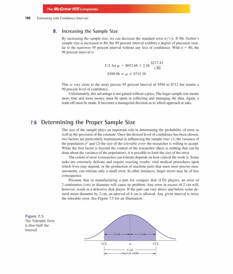
Version, Third Edition
180 Estimating with Confidence Intervals
B. Increasing the Sample SizeBy increasing the sample size, we can decrease the standard error s� . If Mr. Gerber’ssample size is increased to 80, the 99 percent interval exhibits a degree of precision simi-lar to the narrower 95 percent interval without any loss of confidence. With n � 80, the99 percent interval is
This is very close to the more precise 95 percent interval of $594 to $712 but retains a99 percent level of confidence.
Unfortunately, this advantage is not gained without a price. The larger sample size meansmore time and more money must be spent in collecting and managing the data. Again, atrade-off must be made. It becomes a managerial decision as to which approach to take.
7.6 Determining the Proper Sample SizeThe size of the sample plays an important role in determining the probability of error aswell as the precision of the estimate. Once the desired level of confidence has been chosen,two factors are particularly instrumental in influencing the sample size: (1) the variance ofthe population s2 and (2) the size of the tolerable error the researcher is willing to accept.While the first factor is beyond the control of the researcher (there is nothing that can bedone about the variance of the population), it is possible to limit the size of the error.
The extent of error a researcher can tolerate depends on how critical the work is. Sometasks are extremely delicate and require exacting results: vital medical procedures uponwhich lives may depend, or the production of machine parts that must meet precise mea-surements, can tolerate only a small error. In other instances, larger errors may be of lessconsequence.
Presume that in manufacturing a part for compact disk (CD) players, an error of2 centimeters (cm) in diameter will cause no problem. Any error in excess of 2 cm will,however, result in a defective disk player. If the part can vary above and below some de-sired mean diameter by 2 cm, an interval of 4 cm is allowed. Any given interval is twicethe tolerable error. See Figure 7.5 for an illustration.
$589.96 m $715.39
C.I. for m � $652.68 �$217.43
� 80
� n
2 cm 2 cm
LCL m UCL
4 cmInterval width
Figure 7.5The Tolerable ErrorIs One-Half theInterval
2.58

Version, Third Edition
Chapter Seven 181
The remainder of this section considers the determination of the proper sample sizeunder various conditions.
A. Sample Size for mRecall that the normal deviate Z can be expressed as
This can be rewritten algebraically as
Sample size forintervals of thepopulation mean
[7.9]
where the difference between the sample mean and the population mean ( � m) is theerror. In the example above for the CD players with a tolerable error of 2 cm, Formula (7.9)would be written as
The value of Z depends on the level of confidence required. This leaves only s2 to bedetermined in order to calculate the proper sample size. In the likely event s2 is unknown,it can be estimated by the sample standard deviation s using a pilot sample of any reason-able size (n � 30). The variance calculated from this preliminary sample can then be usedin Formula (7.9).
Assume, for example, that the manufacturer of the disk players wishes to construct a95 percent interval for the mean size of the part. A pilot sample has revealed a standard de-viation of 6 cm. How large should the sample be? A 95 percent interval calls for a Z-valueof 1.96. Thus,
The manufacturer should select a sample of 35 parts. From this sample, a 95 percent inter-val could be constructed for the mean size. This interval would have an error not greaterthan 2 cm.
Example 7.4 The owner of a small ski resort in southern Wisconsin is considering the purchase of asnowmaking machine to assist Mother Nature in providing a proper base for ski enthusi-asts. If the average snowfall seems insufficient, he feels that the machine should soon payfor itself. He plans to estimate the average snowfall in the area, but has no idea how largehis sample should be. He only knows that he wants to be 99 percent confident of his find-ings and that the error should not exceed 1 inch. The owner promises you season lift tick-ets if you can help him.
n �(1.96)2(6)2
(2)2 � 34.5 or 35
n �Z 2 s2
(2)2
X
n �Z2 s2
(X � m)2
Z �X � m
sx
�X � m
s��n

Version, Third Edition
182 Estimating with Confidence Intervals
Solution: You begin with a large (n � 30) pilot sample that produces a standard deviation of3.5 inches. Thus,
or 82 snowfalls over the past several years.
Interpretation: You can now collect the data on 82 past snowfalls that will be used to estimate the averagesnowfall. With this information the owner can determine whether Mother Nature needshelp. More important, you can spend the rest of the winter skiing for free.
B. Sample Size for pIn the Chapter 6, we found that
where
We can rewrite this to produce an expression for sample size.
Sample size for intervalsof the population [7.10]proportion
where (p � p) is the difference between the sample proportion and the population propor-tion, and is therefore the error.
Formula (7.10) requires a value for p. However, p is the parameter we wish to esti-mate, and is unknown. This problem can be handled in one of two ways. We could take apilot sample to obtain a preliminary value for p, as we did in our efforts to determine theproper sample size for the mean. Or, we might merely set p � 0.5 for the purpose of de-termining sample size. This approach is often preferred because it is very “safe” or conser-vative—it will ensure the largest possible sample size given any desired level of confi-dence and error. This larger sample results from the fact that the numerator of Formula(7.10), which contains p(1 � p), will be maximized (thus, n will be maximized) if p �1 � p � 0.5. There is no value other than 0.5 which you could assign to p that wouldmake p(1 � p) larger. If p � 0.5, then p(1 � p) � 0.25. Any value other than 0.5 wouldresult in p(1 � p) � 0.25. Thus, n would be smaller.
Wally Simpleton is running for governor. He wants to estimate within 1 percentagepoint the proportion of people who will vote for him. He also wants to be 95 percent con-fident of his findings. How large should the sample size be?
A sample of 9,604 voters will permit Wally to estimate p within 1 percent at the 95 percentlevel of confidence.
� 9,604 voters
n �(1.96)2(0.5)(0.5)
(0.01)2
n �Z 2(p)(1 � p)
(p � p)2
sp � �p(1 � p)n
Z �p � p
sp
� 81.5
�(2.58)2(3.5)2
(1)2
n �Z 2(s)2
(error)2

Version, Third Edition
Chapter Seven 183
Example 7.5 The city council is planning an ordinance prohibiting smoking in all public buildings in-cluding restaurants, taverns, and theaters. Only private housing will be exempt. However,before such an ordinance is brought before the council, this august body wishes to estimatethe proportion of residents who support such a plan. Lacking any statistical skills, the coun-cil hires you as a consultant. Your first step will be to determine the necessary sample size.You are told that your error should not exceed 2 percent and that you must be 95 percentconfident of your results.
Solution: Since no pilot survey was previously taken, you must temporarily set p at 0.5 for the pur-pose of resolving the sample size.
Interpretation: With the data supplied by 2,401 people you can proceed with your estimate of the propor-tion of all residents who might favor the ordinance. The council can then make its deter-mination regarding the citywide smoking policy.
26. Days Inn wants to develop a 99 percent interval for the mean number of rooms occupiedeach night at its locations around the nation. How many nights must be included in thesample if an error of 50 rooms can be tolerated and a pilot sample reveals s � 165 rooms?
27. What would happen to your answer if s � 265? Why?
28. How large a sample is required to provide a 90 percent estimate of the mean number ofgraduates from our nation’s colleges and universities with an error of 2,000 students if a pilotsample reports s � 8,659?
29. A study you are conducting requires a 95 percent interval for the mean rate of return yourfirm earns on its capital budgeting projects. How many projects must you sample if yoursupervisor specifies an interval of only 5 percent and s � 2.3 percent? What is the size of thetolerable error?
30. As a newly hired employee in the marketing division for a large retail concern, you have beenassigned the task of estimating the proportion of consumers who prefer your product over thecompetitor’s. How many consumers must you sample if you want to restrict the error to10 percent and still provide a 99 percent level of confidence?
31. How large must the sample be in the previous problem if the error is restricted to 5 percent?Explain the difference.
32. The credit division for a large commercial bank wants to estimate at the 99 percent level ofconfidence the proportion of its consumer loans that are in default. If the interval width is tobe 7 percent, how many loans must be examined? What is the tolerable error?
7.7 Properties of Good EstimatorsA distinction should be drawn between an estimator and an estimate. An estimator is therule or procedure, usually expressed as a formula, that is used to derive the estimate. Forexample,
X ��Xi
n
� 2,401 citizens
�(1.96)2(0.5)(0.5)
(.02)2
n �Z 2 p(1 � p)
(error)2
Section Exercises

Version, Third Edition
184 Estimating with Confidence Intervals
is the estimator for the population mean. If the value of the estimator is found to be, say,10, then 10 is the estimate of the population mean.
Estimators and Estimates An estimator is the process by which the estimate is ob-tained. An estimate is the numerical result of the estimator.
To perform reliably, estimators must be (1) unbiased, (2) efficient, (3) consistent, and(4) sufficient. Each property is discussed in turn in this section.
A. An Unbiased EstimatorAs we saw in Chapter 6, it is possible to construct a sampling distribution by selecting allpossible samples of a given size from a population. An estimator is unbiased if the mean ofthe statistic computed from all these samples equals the corresponding parameter.
Let u (Greek letter theta) be the parameter we are trying to estimate by (read “thetahat”). Then is an unbiased estimator if its mean, or expected value, E( ), equals u. That is,
To cite a specific example, is an unbiased estimator of m because the mean of thesampling distribution of sample means, equals m. Thus,
Unbiased Estimator An estimator is unbiased if the mean of the sampling distribu-tion equals the corresponding parameter.
Figure 7.6 illustrates how the mean of a sampling distribution must equal the corre-sponding parameter to ensure an unbiased estimator.
E(X ) � X5
� m
X5
,X
E(u) � u
uu
u
X
^E (u 1) = u
u1 u2
u^
E (u2)
Figure 7.6Distributions forBiased andUnbiased Estimators
Here, is an unbiased estimator of u since its distribution is centered over u. Thus,E( ) � u. If many different samples were taken, yielding many different values for ,their mean would equal u. Conversely, if many samples were taken and was calculatedeach time, their mean would exceed u. Thus, is a biased (upward) estimator of u. Themeasure of bias is the difference between the mean of and u. Note that
while
E(u2) � u � 0
E(u1) � u � 0
u2
u2
u2
u1u1
u1

Version, Third Edition
Chapter Seven 185
B. An Efficient EstimatorThe efficiency of an estimator depends on its variance. Let and be two unbiased esti-mators of u. Then is a more efficient estimator if, in repeated sampling with a given sam-ple size, its variance is less than that of . It is only logical that an estimator with a smallervariance will more closely estimate the parameter. Consider Figure 7.7, which shows thesampling distributions with a given sample size of two statistics, and Both and are unbiased estimators of u because their sampling distributions are centered above u, and
However, the variance of the sampling distribution of , is less than that of . Possiblevalues for are more dispersed. Any estimate of u using is likely to produce a largersampling error than an estimate of u using .u1
u2u2
u2u1
E(u1) � E(u2) � u
u2u1u2.u1
u2
u1
u2u1
u
u1
u2
Figure 7.7The Variance ofEstimators
An Efficient Estimator Given any unbiased estimators, the most efficient estimatoris the one with the smallest variance.
C. A Consistent EstimatorAn estimator is consistent when, as n increases, the estimator approaches the value of theparameter.
Consistent Estimator An estimate is consistent if, as n increases, the value of thestatistic approaches the parameter.
For an estimate to be consistent, it must be unbiased and its variance must approach zeroas n increases. The variance of the sampling distribution of the sample means, , is s2�n.As n gets larger, will approach zero. Therefore, it can be said that is a consistent esti-mator of m.
If a statistic is not a consistent estimator, taking a larger sample to improve your esti-mate will prove fruitless.
D. A Sufficient EstimatorAn estimator is sufficient if it uses all relevant information about the parameter containedin the sample. If an estimator is sufficient, nothing can be gained by using any otherestimator.
Xs2x
s2x

Version, Third Edition
186 Estimating with Confidence Intervals
Sufficient Estimator An estimator is sufficient if no other estimator could providemore information about the parameter.
This discussion of estimator properties is by no means a complete account. It does,however, provide a sufficient foundation for an examination of estimating parameters byconstructing confidence intervals.
Solved ProblemsArtesian Spring Water provides bottled drinking water to homes in the tri-county area in 15-galloncontainers. The manager wants to estimate the mean number of containers the typical home uses eachmonth. A sample of 75 homes is taken and the number of containers is recorded. The mean is
with s � 0.78.
a. What would a 92 percent interval reveal?
Solution: The Z-value for a 92 percent interval is found by first dividing 0.92 by 2: as 0.92�2 � 0.46. The areaof 0.46 requires a Z-value of 1.75. Then,
The manager can be 92 percent certain that the mean containers per month is between 3.04 and 3.36.
b. However, the manager feels this interval is too wide. How many homes must he sample to be99 percent confident that the interval is not in error by more than 0.10 containers?
Solution:
A sample of 405 would permit a 99 percent interval, with an error not exceeding 0.10 containers.
c. A smaller sample of 10 homes is selected to estimate the mean number of family members perhouse. The results are 1, 3, 4, 7, 2, 2, 3, 5, 6, and 6 people in each house. What are the resultsof a 99 percent interval for the mean number of family members?
Solution: The sample standard deviation is s � 2.02 with a mean of 3.9. Given the small sample, a t-value oft0.01,9 � 3.250 must be used. Therefore,
d. Of the 75 homes in the sample, 22 have in-home water softeners. What is the 95 percent inter-val estimate of the proportion of all homes in the tri-county area with softeners?
Solution: Since the sample proportion is p � 22�75 � 0.29, the standard error is
sp � �(p)(1 � p)n
� �(0.29)(0.71)75
� 0.052
1.82 m 5.98 people
� 3.9 � (3.250)2.02
�10
C.I. for m � X � tsx
n �Z2s2
(error)2 �(2.58)2 (0.78)2
(0.1)2 � 405
3.04 m 3.36
� 3.2 � (1.75)0.78
�75
C.I. for m � X � (Z)sx
X � 3.2,
Version, Third Edition
Chapter Seven 187
Then,
e. If an interval ranging from 18.8 percent to 39.2 percent of all homes that have softeners lacksprecision, how large a sample must be taken to produce an interval of only 10 percent?
Solution: If the interval is to be 10 percent, the error can be only 5 percent. Then,
List of Formulas[7.1] Confidence interval for m when s
is known
[7.2] Confidence interval for m when s
is unknown
[7.3] Variance for the t-distribution
[7.5] Confidence interval for small samples
[7.7]Estimate of the standard error ofsampling distribubution of sampleproportions
[7.8] Confidence interval for populationproportion
[7.9] Sample size for m
[7.10] Sample size for p
Chapter Exercises33. A 95 percent confidence interval is constructed, yielding a lower confidence limit of 62 and an
upper confidence limit of 69. Can you conclude from this that there is a 95 percent probabilitythe parameter is between 62 and 69? Explain.
34. In a survey of 500 managers, Posner Products found 200 managers lacked sufficient statisticaltraining.
a. What is the point estimate of the proportion of all Posner managers who require addi-tional work in statistical analysis?
b. What is the estimate of the standard error of the proportion?c. What is the 90 percent confidence interval for the population proportion? Interpret your
answer.
35. Jose has a thriving business in Acapulco selling authentic plastic Inca relics to Americantourists. He selects n � 60 days to estimate his daily profit. However, Jose does not knowwhether the population of daily profits is normally distributed, and is uncertain how to pro-ceed. What should he do?
36. As a quality control expert, you want to estimate the mean thickness of optical lenses pro-duced by your firm. A sample of 120 lenses reveals a mean of 0.52 millimeter (mm). The
n �Z 2 (p)(1 � p)
(p � p)2
n �Z 2 s2
(X � m)2
C.I. for p � p � Zsp
sp � �p(1 � p)n
C.I. for m � X � tsx
s2 �n � 1
n � 3
C.I. for m � X � Zsx
C.I. for m � X � Zsx
n �Z 2(0.5)(0.5)
(error)2 �(1.96)2(0.5)(0.5)
(0.05)2 � 385 homes
0.188 p 0.392
� 0.29 � (1.96)(0.052) C.I. for p � p � Zsp

Version, Third Edition
188 Estimating with Confidence Intervals
population standard deviation is known to be 0.17 mm. You feel that you can risk a probabil-ity of error of only 1 percent. Construct the appropriate confidence interval.
37. How would the previous problem change if s was unknown and the sample standard devia-tion was 0.17 mm? Calculate the interval.
38. Georgia Pacific (GP), a major U.S. paper company, decides to harvest a timber stand if it canget an average of at least 700 board feet per tree (bf). A sample of 1,000 trees yields a meanof 695 bf, with a standard deviation of 22.1 bf.
a. Calculate the 90 percent confidence interval.b. Interpret your answer.c. Should GP harvest the stand?
39. In a survey of 6,000 people, U.S. News & World Report found that, in his or her lifetime, theaverage American spends six months sitting at stoplights. Taking this as the sample mean, andassuming the standard deviation is 2.2 months, what is the 90 percent confidence interval forthe population mean? Interpret your answer.
40. The Journal of Retail Management reported that a sample of 600 shoppers spent an average of1.79 hours in a shopping mall per visit. The standard deviation was 0.83 hour. What is the in-terval estimate of the average number of hours all shoppers spend in the mall? Set a � 0.10.
41. Your product requires that a certain component used in its manufacture average 15.2 grams. Ifyou purchase 100 components and find grams, with s � 3.2 grams, what would aconfidence interval tell you about the advisability of buying more from this supplier? Yourproduct is very delicate, and you feel you can tolerate only a 1 percent probability of error.
42. If, given the conditions in the previous problem, the sample had yielded a mean of 14.1 grams,what would you conclude?
43. Wally wants to buy his wife a brand-new septic tank for her birthday. Being a careful shopper,he examines 40 different models and finds a mean price of $712, with a standard deviation of$215. What is the 95 percent confidence interval for the mean price of all septic tanks?
44. A manufacturer of snow skis wants to estimate the mean number of ski trips taken by avidskiers. A sample of 1,100 skiers yields trips per season, with s � 5.1 trips. What isthe 99 percent confidence interval for the population mean?
45. Consider the data in the previous exercise:
a. Without working the problem, explain what would happen to the interval if the level ofconfidence were decreased to 90 percent.
b. Work the problem with a � 0.10 and show how the answer supports your response to part a.
46. A researcher found that a sample of 100, with and s � 10.1, generated a confidenceinterval of 48.3204 to 52.2796. What level of confidence can be attributed to this interval?
47. The weights of 25 packages shipped through United Parcel Service (UPS) had a mean of3.7 pounds and a standard deviation of 1.2 pounds. Find the 95 percent confidence interval forthe mean weight of all packages. Package weights are known to be normally distributed.
48. A sample of 12 donations by political action committees (PACs) to congressional campaignfunds was recorded, in thousands of dollars, as 12.1, 8.3, 15.7, 9.35, 14.3, 12.9, 13.2, 9.73,16.9, 15.5, 14.3, and 12.8. Calculate the 90 percent confidence interval for the mean donationby PACs. Donations are assumed to be normal.
49. The earnings per share for 10 industrial stocks listed on the Dow-Jones were $1.90, $2.15,$2.01, $0.89, $1.53, $1.89, $2.12, $2.05, $1.75, and $2.22. Calculate a 99 percent confidenceinterval for the EPS of all the industrials listed in the DJIA. What assumption must you make?
50. Dr. Bottoms, the local proctologist, found that the average age of 75 of his patients was 47.3with a standard deviation of 10.9 years. Calculate the 99 percent confidence interval for themean age of all his patients under the assumption that the ages are not normally distributed.
51. During the last Superbowl Sunday, Sammy Salami and his buddies ordered 27 pizzas fromPizzas On Wheels. The average delivery time proved to be 23.7 minutes, with a standarddeviation of 10.7 minutes. Feeling this was far too long a delay in their culinary pursuits,
X � 50.3
X � 15.3
X � 14.8

Version, Third Edition
Chapter Seven 189
Sammy and his friends decided to buy the 28th pizza elsewhere if it appeared that the deliverytime for POW exceeded 30 minutes. Set alpha at 1 percent. Will they order elsewhere?
52. A large public accounting firm hired an industrial psychologist to measure the job satisfactionof its senior partners. Seventeen partners were given a test to measure satisfaction; theyscored an average of 83.2 out of a possible 100. From previous studies the firm knows that thetest scores are normal and the variance for all its partners is 120. What is the 90 percent confi-dence interval for the mean score?
53. To estimate how many of the 350,000 residents of Peoria desire a new civic center, the mayorfinds that 1,570 out of the 2,100 residents sampled expressed support. Help the mayor con-struct and interpret the 90 percent confidence interval.
54. Of 209 customers, 183 expressed satisfaction with the banking services offered by First ofAmerica in Peoria, Illinois. How does this compare with the results of an earlier study byRiver Valley Savings, which estimated at the 99 percent level of confidence that somewherebetween 74.1 and 83.7 percent of its customers were satisfied?
55. A textile firm found that it suffered an overall 19 percent waste factor. A new process was im-plemented and a sample of 1,376 units revealed an average waste factor of 11.1 percent, witha standard deviation of 1.12 percent. What conclusion can be made with a 95 percent confi-dence interval about the benefit of the new process?
56. Professional golfers were asked to rate a new graphite club on a scale of 0 to 10. Twenty-fivepros generated a mean rating of 7.3, with s � 1.01. Construct and interpret the 90 percentconfidence interval.
57. Named after Malcolm Baldrige, who served as secretary of commerce in the late 1980s, theBaldrige National Quality Award is a highly sought recognition of a corporation’s commit-ment to a total quality management (TQM) system. Seven criteria are specified by which thecorporations are judged. One such criterion, leadership, allows organizations to collect up to100 points toward achieving this honor. Chrysler Corporation sampled 19 plants and found anaverage of 73.2 points, with s � 10.1. Construct and interpret the 99 percent confidence inter-val for all of Chrysler’s plants.
58. The Pizza Pub is considering increasing the price of its large sausage pizza if the averageprice of its competitors exceeds Pizza Pub’s price of $12.95. Thirty-seven other pizza placesreport a mean price of $12.50, with a standard deviation of $1.01. Pizza Pub wants to be90 percent confident of its findings.
59. In a survey of 673 retail stores, 521 reported a problem with employee thefts. Can you con-clude, with 99 percent confidence, that these data suggest that 78 percent of all stores havesimilar difficulty—as reported in a recent CNN account?
60. Wok and Roll, a Chinese takeout restaurant, wanted to determine what percentage of its cus-tomers chose birds’ nest soup as part of their dining pleasure.
a. In a sample of 320 customers, 220 took home this delicacy. Calculate and interpret the99 percent interval.
b. Using the above data, construct the 90 percent interval.c. Why did you get a smaller interval? Wouldn’t it always be desirable to reduce the interval
width in this manner?
61. The Jesse James First National Bank has hired you as a statistical consultant to analyze opera-tions of its automatic teller machines. A sample of 15 showed mean transactions of $4,810,with a standard deviation of $1,202 per day. Your supervisor insists that you must be 99 per-cent confident of your estimate of the average daily volume. What do you tell her?
62. The owner of a small business wishes to estimate the average time required to complete a cer-tain job task. He must ensure that he is 90 percent confident that the error is less than 0.5 min-utes. The standard deviation is known to be 3.2 minutes. How many observations of comple-tion times must he make?
63. The dean of a private university wants an estimate of the number of out-of-state students en-rolled. She must be 95 percent confident that the error is less than 3 percent. How large a

Version, Third Edition
190 Estimating with Confidence Intervals
sample must she take? If the sample reveals a proportion of 31 percent out-of-staters, andthere are 12,414 students, how many students do you estimate come from other states?
64. The director of a branch bank is asked to estimate the average time a customer spends in thedrive-through facility. He must be 99 percent confident that the estimate is not in error bymore than 15 seconds. How many observations must he collect if the standard deviation isknown to be 2.7 minutes?
65. In an effort to reduce insider trading, the Securities and Exchange Commission (SEC) requestedinformation regarding the proportion of bank holding companies whose officers hold more than50 percent of their banks’ outstanding stock. Of 200 companies selected at random, 79 reportedthat insiders held a majority of their stock. What is the 90 percent confidence interval for theproportion of all bank holding companies whose officers hold at least 50 percent of stock?
66. A researcher for the Federal Aviation Administration (FAA) was quoted in a February issue ofThe Washington Post as saying that, of 112 airline accidents, “73 involved some type of struc-tural problem with the aircraft.” If these figures are representative, what is the confidenceinterval for the proportion of accidents involving such a structural defect? Set a � 0.01.
67. United Airlines surveyed 93 passengers on a flight from Cincinnati to Atlanta. Sixty-four saidthey would like to have been on a later flight had space been available. United had decidedthat if more than 50 percent of the passengers expressed interest in departures later in the day,they would consider making such flights available. Given the results of the survey, does a90 percent confidence interval suggest they should do so?
68. The Wall Street Journal reported efforts by Nestlé, the world’s largest food company, to intro-duce a new product. Management decided to use the Chicago area as a test market. If morethan 30 percent of the people expressed a desire for the product, they would consider market-ing it in a wider area. Of 820 people tested, 215 expressed a positive reaction. Would a 90 per-cent confidence interval for the proportion of all consumers who prefer the product encouragemanagement to continue with their marketing plans?
69. Business Week carried a story about efforts by the 12 member countries of the Common Mar-ket to curtail a growing wave of mergers thought to be “economically undesirable to interna-tional interests.” A sample is to be selected to estimate the mean size of firms (as measured incorporate net worth) involved in mergers. If the interval is to be $5.2 million and carry a levelof confidence of 95 percent, how large should the sample be if the standard deviation ofcorporate net worth is deemed to be $21.7 million?
70. Your division director requests that you, as a newly hired marketing analyst, estimate averageweekly sales. He cautions you to keep your error within $100 and retain a 90 percent level ofconfidence. How many weeks of data must you collect if the standard deviation is $750?
71. A survey of violence in schools is designed to estimate the percentage of male students whowere threatened with violence on school grounds over the past year. The tolerable error is setat 1 percent, and the level of confidence is to be 99 percent. What is the proper sample size?
72. The Student Finance Association at Faber College is planning a “spring fling,” at which theyintend to sell T-shirts imprinted with their logo. The treasurer wants an estimate of the propor-tion of students who will buy one of the T-shirts. The estimate is to provide a 90 percent levelof confidence and the error should not exceed 3 percent. How large a sample must be taken?
73. If a manufacturer wishes to develop a 99 percent interval of the proportion of defects that is inerror by less than 1 percent, how large a sample is required?
Computer ExerciseTelmark Technologies recently instituted new company goals to increase the average size of sales percustomer and to improve the service offered their customers. Last quarter sales averaged $373.10 percustomer order and it took an average of 4.5 days to delivery the shipment to the customers. Inaddition, top executives at Telmark want to reduce the average weight of shipments below the meanof 55.8 pounds to decrease shipping costs. Hal Ketchum, Vice-President for Product Relations, has

Version, Third Edition
Chapter Seven 191
been charged with the responsibility of achieving these objectives. He directs his statistical staff tocollect the necessary data and prepare a report detailing the current conditions.
Access the file TELMARK from your data disk. It contains data for sales orders from 75 cus-tomers. The size of sales in hundreds of dollars is recorded as Size, the number of days each order tookto be shipped to the customers is recorded as Days and the variable Weight provides data for the weightsof the shipments in pounds. Finally, the variable SAT indicates whether the customer was satisfied withthe service from Telmark. It is encoded as a “1” if the customer was satisfied and a “0” if not satisfied.
Using the data in the TELMARK file, provide interval estimates for Size, Days and Weight ofshipments. What conclusions do you reach? Compute the interval estimate for the proportion of sat-isfied customers. Present your finalized statistical report as described in the appendix. Include all rel-evant findings, conclusions and recommendations.
C U R T A I N C A L LFor many years the Fed-eral Bureau of Investiga-tion has served as a model
for law enforcement agencies. Revolution-ary efforts by the FBI to more fully integratethe use of statistical analysis in crime fight-ing efforts were mentioned in Setting theStage at the beginning of this chapter.
The statistical-based approach to crimefighting includes data on a wide variety ofcrimes as well as the personal characteristicsand habits of the offenders. Although thespokesperson on Larry King Live offered nospecifics, she stated that data were kept onthe number of crimes each lawbreaker com-mits, the number of days that pass betweencrimes, and the number who are killed bylaw enforcement in the arrest attempt.
Let us assume that the data for a sampleof 1,000 felons are collected. The data revealthat, on the average, criminals commit 12.4unlawful acts with a standard deviation of 4.7before finally being apprehended or killed. Inaddition, the data report that an average of
19.6 days lapse between criminal acts, with astandard deviation of 11.5 days. In addition,212 of the 1,000 felons in the database losttheir lives trying to elude police.
Assume further that a smaller sampleof a specific type of criminal is taken. Fif-teen observations for armed robbery reportthe following amounts, in thousands of dol-lars, were taken in the robbery: 45.6, 23.8,45.3, 27.9, 54.3, 27.5, 63.4, 12.6, 75.9, 64.6,54.7, 17.5, 21.4, 56.4, and 34.9.
Based on these data and the toolslearned in this chapter, provide a profile ofcriminal activity across the nation like thatyou think a statistician for the FBI mightprepare. Select and justify your own levelsof confidence, and calculate and interpret allconfidence intervals. Comment on the sam-ple sizes. Are they sufficient to achieve yourobjective? Clearly specify what samplesizes are needed to achieve the level of con-fidence and tolerable error you require. Pre-sent your final account in the form of a busi-ness report as described in Appendix I.
From the Stage to Real LifeThe FBI web site (www.fbi.gov) provides selected crime statistics similar to those used inthe Curtain Call analysis. From the FBI home page, click on “Publications.” Under theUniform Crime Statistics heading, click on “Final 19xx Crime Statistics” (most recent fullyear data). Make a list of the categories of crime statistics available at this site.
Look up information on burglary and on aggravated assaults. Note both the crimecounts and the rate per 100,000 population for these two categories. What information isgiven on the increase or decrease in the type of crime over the previous year? Are these dataa sample or a census? Does the available data provide enough detail for you to test if thechange from the previous year is statistically significant? If not, what further informationwould you need to construct such a test?

Version, Third Edition
192
C H A P T E R8Hypothesis Testing

Version, Third Edition
193
Hypothesis Testing
The concept ofhypothesis testing
Critical Z-valuesand rejection regions
Probabilityof error
Formulating thedecision rule
Testing the hypothesisabout the population mean
One-tailed andtwo-tailed tests
p-values
Small sampletests for m
Tests for p
One-tailed andtwo-tailed tests
p-values
Chapter BlueprintA hypothesis is an assumption or an inference about the unknown value of a parameter. This chapterexamines how we can test hypotheses and thereby draw some conclusions about the population.

Version, Third Edition
S E T T I N G T H E S T A G E
8.1 IntroductionThe purpose of statistical analysis is to reduce the level of uncertainty in the decision-making process. Business managers can make better decisions only if they have more in-formation at their disposal. Hypothesis testing is a very effective analytical tool for obtain-ing this valuable information under a wide variety of circumstances. Common businessexamples abound:
194 Hypothesis Testing
Over the past several yearsthe American banking sys-tem has undergone consid-
erable deregulation. Much of this deregula-tion has come in the form of the relaxationof laws governing the performance and op-erations of commercial banks and other fi-nancial institutions. First Bank of Americahas just merged with Great Lakes National,a smaller competitor in the Midwest, andmanagement is planning several policychanges that could dramatically affect bank-ing operations (Chicago Tribune, June 5,1997).
Lawrence Hopkins, divisional man-ager of customer relations, has been chargedwith the responsibility of providing esti-mates of many of the important indicators ofconsumer attitudes toward these anticipatedchanges. Of special concern is the bank’s
intention to base fees and other charges onthe depositor’s average daily checking ac-counts balance. Due to the merger, the bankfeels its market position is strong enoughto impose a fee increase without unduecustomer backlash. Records show thataverage deposits have been rising and thatFirst Bank has gained a larger market shareover the past two years relative to theirtwo biggest remaining competitors, MagnaBank and City National. As the graphshows, First Bank’s share of total bank de-posits in the fourth quarter of 1998 (1998-IV) is estimated to be 70 percent.
This chapter explores the tools that canbe used to prepare a report that could provevery beneficial in making many of the deci-sions First Bank must address in its effort tocontinue the success and prosperity it hasenjoyed over the past several years.
50
40
30
20
10
0
60
70
CITY
Percentage of Total Deposits
Market Share
1998-IV1998-III1998-II1998-I1997-IV1997-III1997-II1997-I
FIRST MAGNA
Version, Third Edition
Chapter Eight 195
● A bottler of soft drinks must determine whether the mean fill-weight in its bottles is16 ounces (m � 16 ounces).
● A producer of computer software wishes to certify that the proportion of its productsthat are defective is less than 3 percent (p � 0.03).
● A manufacturer of sports equipment wants to see whether there is evidence that a pro-duction process has reduced mean production costs below their current level of $5 perunit (m � 5).
Illustrations of this nature are virtually limitless in a business setting. If answers to thesequestions and many others like them can be obtained with some degree of assurance, deci-sion making becomes more certain and less likely to lead to costly error.
8.2 The Concept of Hypothesis TestingTo conduct a hypothesis test, we make some inference or educated guess about the popula-tion. The bottler of soft drinks cited above may assume, or hypothesize, that the mean fillis 16 ounces (m � 16). This null hypothesis (H0:) is tested against the alternative hy-pothesis (HA:) stated to the contrary. In this case the mean fill is not 16 ounces (m � 16).Thus, we would have
H0: m � 16 HA: m � 16
The word null implies none or nil. The term arises from its earliest applications byagricultural researchers who tested the effectiveness of a new fertilizer to determine its im-pact on crop yield. They assumed that the fertilizer made no difference in yield until itcaused some effect. Thus, the null hypothesis traditionally contains some reference to anequal sign such as “ � ”, “ � ”, “ ”. We explore this idea more fully later in our discus-sion of one-tailed hypothesis tests.
Based on sample data, this null is either rejected or not rejected. We can never “accept”the null as true. Failure to reject the null only means that the sample evidence is not strongenough to lead to its rejection. Even if � 16, it does not prove that m � 16. It could bethat m is 15.8 (or anything else), and due to sampling error the sample mean just happenedto equal the hypothesized value of 16. An analogy is that testing a hypothesis is like puttinga person on trial. The accused is found either guilty or not guilty. Never is a verdict of“innocent” handed down. A not-guilty verdict simply means the evidence is not strongenough to find the defendant guilty. It does not mean that he or she is innocent.
When conducting a hypothesis test, the null is presumed “innocent” (true) until a pre-ponderance of evidence indicates that it is “guilty” (false). Just as in a legal setting, theevidence of guilt must be established beyond any reasonable doubt. Before the null isrejected, the sample mean must differ from the hypothesized population mean significantly.That is, the evidence must be quite convincing and conclusive. A conclusion based on arejection of the null is more meaningful than one that results in a decision to not reject.
Presume that we take a sample of n bottles and find a mean of � 16.15 ounces. Canwe conclude the population mean is not 16? After all, 16.15 is not 16! Probably not. Thissmall difference could be statistically insignificant in that it could easily be explained awayas a mere sampling error. That is, due to sampling error it may be possible to enter a popu-lation with a mean of 16 and emerge with a sample mean of � 16.15. Due to the luckof the draw, some of the bottles in the samples may have been somewhat overfilled, caus-ing the sample mean to slightly overestimate the population mean. The sample evidence
� 16.15 is not strong enough to lead to a rejection of the null hypothesis that m � 16.X
X
X
X

Version, Third Edition
196 Hypothesis Testing
Statistically Insignificant Difference A difference between the hypothesized popu-lation mean and the sample mean that is small enough to attribute to sampling error.
If the difference between the hypothesized mean of 16 and the sample finding of 16.15is insufficient to reject the null, the question then becomes just how large the differencemust be to be statistically significant and to lead to a rejection of the null. Recall from ourdiscussion of sampling distributions that we can transform any unit of measurement, suchas the ounces for the bottler, to corresponding Z-values with the Z-formula:
If s is unknown, the sample standard deviation s is used.The resulting normal distribution of Z-values has a mean of zero and a standard devi-
ation of one. The empirical rule tells us 95 percent of the ’s in the sampling distributionare within 1.96 standard errors of the unknown population mean, as shown in Figure 8.1.
X
Z �X � m
sx�
X � m
s
�n
0– 1.96 1.96
m = 16
Z-values
0.4750 0.4750
0.95
Left-tailedrejectionregion
Right-tailedrejectionregion
a/2 = 0.025 a/2 = 0.025
Do NotReject
X (ounces)–
Do-Not-Reject Region
There is a 95% chance sampleresults could fall anywherebetween ± 1.96 if thenull is true.
If m = 16, there is onlya 2.5% chance a samplemean could produce a Z-value � –1.96.
H0: m = 16HA: m ≠ 16
If m = 16, there is onlya 2.5% chance a samplemean could produce a Z-value �1.96.
Figure 8.1Critical Values for Zand the RejectionRegions
A. Critical Z-Values and the Rejection RegionsThese Z-values of �1.96 are the critical values indicating the rejection regions. To findthem, divide the 95 percent by 2. From the Z-table, the area of 0.95�2 � 0.4750 producesa Z-value of 1.96. The remaining 5 percent is distributed in the two tails, with 2.5 percentin each rejection region. This 5 percent is the level of significance, or the alpha-value, ofthe test.
In Figure 8.1 note that if the bottler’s hypothesis is correct and m � 16 ounces, it is un-likely (only a 5 percent chance) that any sample could produce a Z-value falling in either

Version, Third Edition
Chapter Eight 197
rejection region. Thus, if a Z-value greater than 1.96 or less than �1.96 does occur, it is un-likely that the distribution is centered at m � 16, and the null should be rejected.
These critical Z-values of �1.96 allow us to establish a decision rule that tells uswhether to reject the null. The decision rule is:
Decision Rule Do not reject the null if the Z-value is between �1.96. Reject if theZ-value is less than �1.96 or greater than �1.96.
The logic behind this decision rule, which is based simply on probabilities, should be clear.If the null is true, it is unlikely that a Z-value greater than 1.96 or less than �1.96 couldpossibly result. Only 5 percent of all the samples in the sampling distribution could pro-duce a Z-value greater than 1.96 or less than �1.96. Therefore, if such a Z-value occurs, itis unlikely that m � 16, and the null should be rejected.
B. The Level of Significance and the Probability of ErrorIn testing a hypothesis, we can make two types of mistakes. A Type I error is rejectinga true hypothesis. In Figure 8.1, if the bottler’s hypothesis is true and m � 16, there isstill a 5 percent chance that a sample mean could fall in either rejection region, causingus to incorrectly reject the null. Of all the sample means in the sampling distribution,2.5 percent produces a Z-value 1.96 in the right-tailed rejection region and 2.5 percentproduces a Z-value � �1.96 in the left-tailed rejection region. This 5 percent is thelevel of significance, or alpha-value ( -value) and represents the probability of a Type Ierror.
Type I Error Rejecting a true hypothesis. The probability of a Type I error equals thelevel of significance, or a-value, at which the hypothesis is tested.
A Type II error is not rejecting a false hypothesis. If the null hypothesis H0: m � 16is not correct, but our test fails to detect this, we commit a Type II error. While the proba-bility of a Type I error is equal to the selected alpha value, the probability of a Type II error,signified as b, is not easily determined. We cannot assume that a � b � 1.
Levels of significance, or a-values, commonly selected for hypothesis tests are 10 per-cent, 5 percent, and 1 percent. However, as with confidence intervals, there is nothing spe-cial or magical about these alpha-values. We could test a hypothesis at the 4 percent levelof significance if we chose to. The selection of an alpha-value depends on which error,Type I or Type II, we most want to avoid. Recall that the alpha-value of the test is the prob-ability of a Type I error. If rejecting a true hypothesis (Type I error) is more serious than notrejecting a false hypothesis (Type II error), you would want to choose a low alpha-value,such as 1 percent or 5 percent, to minimize the probability of committing a Type I error. Onthe other hand, if not rejecting a false hypothesis (Type II error) is more serious, a higheralpha-value, such as 10 percent, might be preferable.
Assume that the soft-drink bottler rejects the null H0: m � 16 and shuts down the bot-tling process to adjust the fill level. If the mean is indeed 16 ounces, however, the bottlerhas committed a Type I error. If this is more costly than a Type II error, allowing the processto continue when , the bottler would want to select a low alpha-value, such as 1 per-cent, for the test.
m � 16
a

Version, Third Edition
8.3 A Two-Tailed Test for mWe are now ready to conduct the hypothesis test. There are four steps involved in the test:
Step 1: State the hypotheses.
Step 2: Based on the sample results, calculate the value of the test statistic, Ztest.
Step 3: Determine the decision rule based on the critical Z-values.
Step 4: Note the findings and conclusion.
Presume that the bottler wants to test the hypothesis that the population mean is 16ounces and chooses a 5 percent level of significance. Since it is hypothesized that m � 16,the null and alternative hypotheses are
To test the hypothesis, the test statistic, Ztest, is calculated and compared to the criticalZ-values.
[8.1]
where is the sample meanmH is the hypothesized value for the population mean
is the standard error of the sampling distribution
When s is unknown, we use the sample standard deviation and the Ztest becomes
[8.2]
where s is the sample standard deviation.If the bottler selects a sample of n � 50 bottlers with a mean � 16.357 ounces and
a standard deviation of s � 0.866 ounces, the Ztest is
In Figure 8.2, the level of significance of 5 percent is divided in the two tails. Theremaining 95 percent is divided by 2 to find the area of 0.4750. From the Z-table this areaof 0.4750 yields critical Z-values of �1.96. The decision rule becomes
Decision Rule Do not reject the null if �1.96 Ztest 1.96. Reject if Ztest ��1.96 or Ztest 1.96.
� 2.91
Ztest �16.357 � 16
0.866
�50
X
Ztest �X � mH
s
�n
s��n
X
Ztest �X � mH
s
�n
HA: m � 16
H0: m � 16
198 Hypothesis Testing
The Ztest-value used totest the hypothesiswhen s is unknown
The Ztest-value used totest the hypothesiswhen s is known

Version, Third Edition
Chapter Eight 199
0– 1.96 1.96
16.357
2.91
16
Z
0.025 0.025
X (ounces)–
Do-Not-Reject Region
H0: m = 16HA: m ≠ 16
Left-tail rejectionregion Right-tail
rejection region
If m = 16, it is unlikelya Z test 1.96 couldresult. Thus, the nullH0: m = 16 is rejected.
0.4750
0.95
0.4750
Figure 8.2Hypothesis Test forthe Mean Fill Level
Notice the rejection regions in both tails. If Ztest 1.96 or Ztest � �1.96, the null is rejected.For this reason this is referred to as a two-tailed test.
The final step in the hypothesis test is to note the findings and determine whether thenull should be rejected. Our sample findings of 16.357 ounces produced a Ztest � 2.91 1.96 and fall in the right-tailed rejection region. We may interpret these results as “the nullis rejected at the 5 percent level of significance.” It just isn’t likely that a population with amean of 16 could yield a sample that would produce a Ztest 1.96. There is only a 2.5 per-cent probability that Ztest could exceed 1.96 (and only a 2.5 percent chance that Ztest ��1.96) if m is really 16. Thus, the null hypothesis H0: m � 16 should be rejected at the5 percent level of significance.
Does this mean that m is not 16? Not at all. If m � 16, 2.5 percent of all the samples ofsize n � 50 would still generate a Ztest 1.96. The population mean could be 16, in whichcase we have committed a Type I error by rejecting it. But this is not likely since P(Ztest 1.96 }m � 16) is only 2.5 percent.
Display 8.1Z-Test
Test of mu � 16.000 vs mu not � 16.000The assumed sigma � 0.866
Variable N Mean StDev SE Mean Z P-ValueOunces 50 16.357 0.866 0.122 2.91 0.0037
The Minitab printout in Display 8.1 provides the results of this test. Assuming 50observations are entered in column 1, merely click on STAT Basic Statistics 1-Sample Z, and enter 16 for Test Mean and the standard deviation for our sample dataof 0.866. Notice that the sample mean, standard deviation, and Z-value of 2.91 are given.We will discuss the all-important p-value later.
Example 8.1 As noted in “Setting the Stage” at the opening of this chapter, management at First Bankof America is planning to base the fees charged for checking accounts on their averagedaily balances. The senior accounts manager wants to test the hypothesis that the accountsaverage $312. A sample of 200 accounts is selected, yielding a mean of $298.10 with

Version, Third Edition
200 Hypothesis Testing
s � $97.30. To minimize the probability of a Type I error, an alpha-value of 1 percent ischosen. (Notice the four steps in conducting the test.)
Solution: The null and alternative hypotheses are
The Ztest is
As the accompanying figure shows, an a � 0.01 requires critical Z-values of �2.58.The 0.01 is evenly divided in the two rejection regions, leaving an area of 0.4950 whichcorresponds to critical Z-values of �2.58.
Ztest �X � mH
s
�n
�298.10 � 312
97.30
�200
� �2.02
HA: m � 312
H0: m � 312
Decision Rule Do not reject if �2.58 Ztest �2.58. Reject if Ztest � �2.58or Ztest 2.58.
If the null is true, there is only a 1 percent chance that a sample could result in a Ztest valueless than �2.58 or greater than 2.58. Thus, if Ztest falls in either tail, it is unlikely thatm � 312 and the null should be rejected. Our Ztest � �2.02 is in the do-not-reject region.
Interpretation: The difference between the hypothesized value of $312 and the sample findings of $298.10is statistically insignificant. It could result merely from sampling error. In fact, ifm � $312, 99 percent of all the samples of size n � 200 would produce Ztest values be-tween �2.58. Thus, a value of �2.02 is not unexpected.
1. What are the four steps to a hypothesis test?
2. Explain in your own words why the decision rule should be used to determine whether thenull should be rejected. What is the role of probability in this decision?
3. What is meant by an “insignificant difference” between the hypothesized population meanand the sample mean?
0– 2.58 – 2.02 2.58
312298.10
Z
0.005 0.005
X (dollars)–
Do-Not-Reject Region
0.4950 0.4950
Section Exercises

Version, Third Edition
Chapter Eight 201
4. Why can we never “accept” the null as true?
5. What role do the critical Z-values perform in the testing process? How are they determined?Draw a graph in your response.
6. What is the “level of significance” in a test? How does it influence the critical Z-values? Drawa graph in your response.
7. Distinguish between a Type I error and a Type II error. Give an example.
8. Using a graph, clearly illustrate how the probability of a Type I error is equal to the level ofsignificance (a-value) of a test.
9. If a Type II error is considered more serious in a certain situation, would you choose a high ora low alpha value? Explain.
10. As the purchasing manager for a large insurance firm, you must decide whether to upgradethe office computers. You have been told that the average cost of desktop computers is$2,100. A sample of 64 retailers reveals a mean price of $2,251, with a standard deviation of$812. At the 5 percent level of significance, does it appear that your information is correct?
11. Enticed by commercials, you have been persuaded to purchase a new automobile. You thinkyou will have to pay $25,000 for the car you want. As a careful shopper, you price 40 possiblevehicles and find a mean cost of $27,312, with a standard deviation of $8,012. Wishing toavoid a Type II error, you test the hypothesis that the mean price is $25,000 at the 10 percentlevel of significance. What is your conclusion?
12. Due to excessive commute times, the office where you work in downtown Chicago is consid-ering staggered work hours for its employees. The manager feels that it takes an average of50 minutes for employees to get to work. Seventy employees average 47.2 minutes with astandard deviation of 18.9 minutes. Set alpha at 1 percent and test the hypothesis.
13. In 1997 the investment firm of Goldman Sachs reported that Americans invest an average of$18.6 million every month in the bond market. Is this claim supported at the 5 percent level ifa sample of 36 months finds a mean of $17.1 million and a standard deviation of $2.4 million?
14. Returning home from the mines, the seven dwarfs tell Snow White that they excavate aweekly average of 12 tons of gold. Unwilling to believe this without proof, Miss White col-lects data for 49 weeks and finds a mean of 11.5 tons and a standard deviation of 1.1 tons. At the 10 percent level does it appear that the dwarfs are correct?
15. Before publishing a new cookbook, Bantam Books wants to test the hypothesis at the 2 per-cent level of significance that the average price of such books is $35.00. Is this claim sup-ported if a sample of 50 cookbooks has a mean of $32.97 and a standard deviation of $12.87?
16. The local supermarket spent many weeks and thousands of dollars remodeling. Although thedisruption temporarily drove away customers, the store manager hopes that the customerswill now return to enjoy the new conveniences. Before the remodeling, store receipts aver-aged $32,533 per week. Now that the remodeling has been completed, the manager takes asample of 36 weeks to see whether the construction in any way affected business. A mean of$34,166 is reported and the standard deviation is $12,955. At the 1 percent level, what can themanager decide?
8.4 One-Tailed Tests for mThe tests conducted above were all two-tailed tests because there were rejection regions inboth tails. As Figure 8.3(A) shows, the test of the bottler’s hypothesis that m � 16 wouldbe rejected if the sample findings are either too high or too low. Either way, it appears thatm is not 16 and the null is rejected.
However, there are times when we are interested in only one extreme or the other. Afresh seafood restaurant in Kansas City is not concerned about how quickly the lobsters

Version, Third Edition
202 Hypothesis Testing
arrive from the East Coast. They worry only if it takes too long for the shipment to arrive.A retail outlet will become alarmed only if revenues fall to disturbingly low levels. Partic-ularly high sales are no problem. In each of these cases, concern is focused on one extremeor the other and a one-tailed test is conducted.
Instead of hypothesizing that the mean fill level is exactly 16 ounces, suppose our bot-tler feels that the mean fill level is “at least 16 ounces.” The null hypothesis becomes H0:
� 16; that is, 16 or more. The alternative hypothesis is stated to the contrary, and theentire set of hypotheses is
Figure 8.3(B) shows that the hypothesis H0: m � 16 is not rejected if the sample findingsare above 16. The hypothesis H0: m � 16 allows for values above 16. Sample means suchas 16.3 or 16.5 or even 17 and 18 support, not refute, the claim that m � 16. Only valuessignificantly below 16 can cause a rejection of the null. Thus, a rejection region appears inonly the left tail and the full amount of the alpha-value is placed in this single rejectionregion.
H0: m � 16 HA: m � 16
m
Figure 8.3A Comparison ofTwo-Tailed andOne-Tailed Tests
0– 1.96 1.96
16
Z
a/2 = 0.025 a/2 = 0.025
X (ounces)–
Do-Not-Reject Region
A two-tailed testhas a rejectionregion in bothtails.
H0: m = 16HA: m ≠ 16
(a)
16 16.3 16.5
a
X (ounces)–
A left-tailed testhas a rejectionregion in onlythe left tail.
H0: m � 16HA: m � 16
(b)
RejectionRegion
Do-Not-Reject Region
16
a
X (ounces)–
A right-tailed testhas a rejectionregion in onlythe right tail.
H0: m 16HA: m 16
(c)
RejectionRegion
Do-Not-Reject Region
1514

Version, Third Edition
Chapter Eight 203
Presume the bottler claims that the mean fill level “is at most 16.” The null is nowwritten as H0: m 16. The hypotheses are
Figure 8.3(C) shows that now low values for the sample findings will not result in a rejec-tion. The null hypothesis H0: m 16 permits findings below 16. Sample means such as 15or even 14 support the claim that m 16. Only values significantly above 16 will cause arejection. Thus, there is a rejection region in only the right tail. The full value for alpha isplaced in this single rejection region.
Notice that in both a left-tailed and a right-tailed test, the equals sign is placed in thenull hypothesis. This is because the null hypothesis is being tested at a specific alpha value(such as 5 percent) and the equals sign gives the null a specific value (such as 16) to test.Example 8.2 illustrates a one-tailed test.
Example 8.2 In a monthly briefing to the corporate office, the manager for the Embassy Suites hotel inAtlanta reports that the mean number of rooms rented out per night is at least 212. That is,m � 212. One of the corporate officials feels that this number might be somewhat over-stated. A sample of 150 nights produces a mean of 201.3 rooms and a standard deviationof 45.5 rooms. If these results suggest the manager has “padded” his report, he will beseverely admonished. At the 1 percent level, what is the manager’s fate?
Solution: The manager’s statement that m � 212 contains the equals sign and thus serves as the nullhypothesis:
H0: m � 212 HA: m � 212
H0: m 16 HA: m 16
Values above 212 will not cause us to reject the null, which clearly allows for values inexcess of 212. Only values significantly below 212 will lead to a rejection of m � 212.Thus, this is a left-tailed test. The Ztest is
Ztest �201.3 � 212
45.5
�150
� �2.88
0– 2.33– 2.88
212201.3
Z
a = 0.01
X (rooms)–
0.4900

Version, Third Edition
204 Hypothesis Testing
As the figure shows, a 1 percent level of significance leaves an area of 0.4900 that, from theZ-table, calls for a critical Z-value of �2.33. The decision rule is
Decision Rule Do not reject if Ztest � �2.33. Reject if Ztest � �2.33.
The Ztest of �2.88 is clearly in the rejection region. The null hypothesis H0: m � 212 isnot supported.
Interpretation: It appears the manager has overstated his occupancy rate and will apparently receive areprimand from the home office.
Consider this next right-tailed test.
Example 8.3 A survey by the National Collegiate Students’ Association showed that students at ournation’s colleges and universities spend on average more than $75 a month for general en-tertainment. If you can find evidence to support this claim, you intend to use it to requestadditional support money from home. From 100 students you sample, you find a mean of$80.23 with a standard deviation of $45.67. At the 2 percent level of significance, have youfound justification for your request?
Solution: The claim that the mean is more than $75.00 serves as the alternative hypothesis sincem 75 does not contain the equal sign. The hypotheses are then
and a right-tailed test is required since lower values would not result in a rejection of thenull. Then,
Ztest �80.23 � 75
45.67
�100
� 1.15
H0: m 75 HA: m 75
The area shown in the figure of 0.4800 indicates a critical Z-value of 2.05. The decisionrule is
Decision Rule Do not reject if Ztest 2.05. Reject if Ztest 2.05.
0 1.15 2.05
75 80.23
Z
a = 0.02
X (dollars)–
0.4800

Version, Third Edition
Chapter Eight 205
Since Ztest � 1.15 � 2.05, the null H0: m 75 is not rejected. It appears that the mean costof entertainment is not more than $75.
Interpretation: Despite your decadent lifestyle, the typical student does not spend more than $75. You aregoing to have to find another way to squeeze more money from home.
17. Explain the difference between one-tailed and two-tailed hypotheses tests in your own words.Give examples of both.
18. Why does the equals sign always go in the null hypothesis?
19. Explain clearly why a null hypothesis of H0: m 10 requires a right-tailed test, while a nullhypothesis of H0: m � 10 requires a left-tailed test.
20. Over the past several months Raynor & Sons has heavily advertised its electrical supply busi-ness. Mr. Raynor hopes that the result has been to increase mean weekly sales above the$7,880 the company experienced in the past. A sample of 36 weeks shows a mean of $8,023with a standard deviation of $1,733. At the 1 percent level of significance, does it appear theadvertising paid off?
21. In the fall of 1997, Hardee’s, the fast-food giant, was purchased by a company in Californiathat plans to remove the fried-chicken line from the menu. The claim was that recently rev-enues have slipped below the $4,500 mean they displayed in the past. Does this seem like awise decision if 144 observations reveal of mean of $4,477 and a standard deviation of$1,228? Management is willing to accept a 2 percent probability if committing a Type Ierror.
22. According to The Wall Street Journal (May 12, 1997) many sportswear companies are tryingto market to the younger age groups. The article suggested that the mean age of the con-sumers has fallen below the 34.4 years that characterized the earlier part of the decade. If asample of 1,000 customers reports a mean of 33.2 years and a standard deviation of 9.4, whatdo you conclude at the 4 percent level of significance?
23. The July 1997 issue of Forbes reported on exclusive “hideaways” in upper New York Stateand surrounding areas used by rich executives to escape the tedium of their stressful dailylives. The cost is quite reasonable, the article reported. You can hire weekend accommoda-tions for less than $3,500. Is this “reasonable” figure supported at the 5 percent level if a sam-ple of 60 resorts average $3,200 and s � $950?
24. In the early 1990s, Hyundai, the Korean automobile manufacturer, suffered a severe drop insales below its monthly peak of 25,000 units in May 1988. Hyundai Motor America (Summer1997) reported that sales had slipped to less than 10,000 units. During a 48-month periodstarting in January 1990, the average sales were 9,204 units. Assume a standard deviation of944 units. At the 1 percent level, does it appear that the mean number of units has fallenbelow the 10,000 mark?
25. Baskin-Robbins, the ice-cream franchise, claims that the number of outlets it opens has in-creased above the weekly mean of 10.4 experienced in leaner times (The Wall Street Journal,February 1997). Is there evidence to support this claim if 50 weeks show a mean of 12.5 anda standard deviation of 0.66 outlets? Management is willing to accept a 4 percent probabilityof rejecting the null if it is true.
26. A recent advertisement claims that the amount of property and marine insurance written byAtlantic Mutual is at least $325,500 per month. Forty months report a mean of $330,000 ands � $112,300. At the 5 percent level of significance, does Atlantic Mutual’s claim seem to bevalid?
Section Exercises
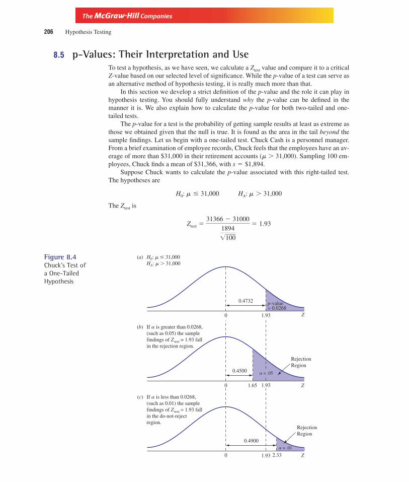
Version, Third Edition
206 Hypothesis Testing
8.5 p-Values: Their Interpretation and UseTo test a hypothesis, as we have seen, we calculate a Ztest value and compare it to a criticalZ-value based on our selected level of significance. While the p-value of a test can serve asan alternative method of hypothesis testing, it is really much more than that.
In this section we develop a strict definition of the p-value and the role it can play inhypothesis testing. You should fully understand why the p-value can be defined in themanner it is. We also explain how to calculate the p-value for both two-tailed and one-tailed tests.
The p-value for a test is the probability of getting sample results at least as extreme asthose we obtained given that the null is true. It is found as the area in the tail beyond thesample findings. Let us begin with a one-tailed test. Chuck Cash is a personnel manager.From a brief examination of employee records, Chuck feels that the employees have an av-erage of more than $31,000 in their retirement accounts (m 31,000). Sampling 100 em-ployees, Chuck finds a mean of $31,366, with s � $1,894.
Suppose Chuck wants to calculate the p-value associated with this right-tailed test.The hypotheses are
The Ztest is
Ztest �31366 � 31000
1894
�100
� 1.93
H0: m 31,000 HA: m 31,000
0 1.93
a = .05
Z
H0: m 31,000HA: m 31,000
(a)
0 1.65 Z
Z
If a is greater than 0.0268,(such as 0.05) the samplefindings of Z test = 1.93 fallin the rejection region.
(b)
0
If a is less than 0.0268,(such as 0.01) the samplefindings of Z test = 1.93 fallin the do-not-rejectregion.
(c)
RejectionRegion
RejectionRegion
0.4732
0.4500
0.4900
p-value= 0.0268
1.93
1.93 2.33a = .01
Figure 8.4Chuck’s Test of a One-TailedHypothesis

Version, Third Edition
Chapter Eight 207
The p-value is the area in the tail beyond the sample finding of Ztest � 1.93. As Figure8.4(A) illustrates, a Ztest of 1.93 yields an area of 0.4732. The p-value, the area in the tailbeyond the sample findings of 1.93, is 0.5000 � 0.4732 � 0.0268, or 2.68 percent.
p-Value The lowest level of significance (�-value) at which the null can be rejected.It is the area in the tail beyond the sample findings.
What exactly does this p-value of 2.68 percent tell Chuck? The p-value is defined asthe lowest level of significance (lowest alpha-value) he can set and still reject the null. Forexample, Figure 8.4(B) shows that if � is set at some value greater than 0.0268, such as0.05, the area of 0.4500 calls for a critical Z-value of 1.65. Thus, the sample findings ofZtest � 1.93 fall in the rejection region. On the other hand, as Figure 8.4(C) reveals, if an�-value less than 0.0268 is selected, such as 0.01, the resulting area of 0.4900 specifies acritical Z-value of 2.33 and the sample findings of Z test � 1.93 fall in the do-not-rejectregion. Thus, Chuck can lower the �-value for the test down to 0.0268 without placingthe sample findings in the do-not-reject region. That is, an �-value of 0.0268 is the lowest�-value Chuck can set and still reject the null.
The p-value tells Chuck what decision he would reach at any selected alpha-value.Simply put, if the p-value is less than the alpha-value, the null will be rejected.
Display 8.2Z-Test
Test of mu � 31000 vs mu 31000The assumed sigma � 1894
Variable N Mean StDev SE Mean Z P-ValueAmount 100 31366 1894 189 1.93 0.0268
Minitab Display 8.2 provides the printout for Chuck’s one-tailed test. The Z-valueand p-value he calculated can be easily obtained by clicking on Stat Basic Statistics 1-Sample Z. Set the confidence level and enter the hypothesized value for the mean. Selectgreater than for the alternative. Finally, enter 1894 for sigma. Caution: Many computerprograms report only p-values for two-tailed tests. If you are conducting a one-tailed test,divide the reported p-value by 2 to get the one-tailed value. However, if you follow thedirections above, Minitab will report the one-tailed value.
A. p-Value for Two-Tailed TestsCalculating the p-value of a two-tailed test is quite similar, with a slight twist at the end.Presume that Chuck also suspects that the employees invest an average of $100 each monthin the company’s stock option plan (m � 100). Sampling 100 employees, Chuck finds amean of $106.81 with a standard deviation of $36.60. He now wants to determine the p-value associated with the hypothesis test
The Ztest is
Ztest �106.81 � 100
36.60
�100
� 1.86
H0: m � 100 HA: m � 100

Version, Third Edition
208 Hypothesis Testing
To calculate the p-value, Chuck determines the area in the tail beyond the sample find-ings of Ztest � 1.86. In Figure 8.5 this area is 0.0314. Unlike a one-tailed test, this area mustbe multiplied by 2 to get the p-value. This is necessary because in a two-tailed test thealpha-value is divided into the two rejection regions. The p-value is 0.0314 � 2 � 0.0628.Remember, the p-value is the lowest alpha-value at which the null is rejected. If the alpha-value is set lower than the p-value, the null is not rejected.
Display 8.3Z-Test
Test of mu = 100.00 vs mu not = 100.00The assumed sigma = 36.6
Variable N Mean StDev SE Mean Z P-ValueDollars 100 106.81 36.60 3.66 1.86 0.063
Minitab Display 8.3 shows the results of Chuck’s two-tailed test. Notice that thep-value of 0.063 is for a two-tailed hypothesis and it is not necessary to multiply by 2.
Example 8.4 In May 1997 Congress approved a federal budget containing several provisions for taxcuts. Analysts claimed it would save the average taxpayer $800 per year. Calculate and in-terpret the p-value if a sample of 500 taxpayers shows a mean savings of $785.10 with astandard deviation of $187.33.
Solution:
The Ztest is
The p-value is determined by finding the area beyond the sample findings of �1.78; as thefigure shows, 0.5000 � 0.4625 � 0.0375. Then, 0.0375 � 2 � 0.0750 � p-value.
Ztest �785.10 � 800
187.33
�500
� �1.78
H0: m � 800 HA: m � 800
0 1.86– 1.86
0.0314 0.4686 0.0314
Z
The area of 0.0314must be multipliedby 2 to get thep-value.
H0: m = 100HA: m ≠ 100
Figure 8.5Chuck’s Two-TailedHypothesis Test

Version, Third Edition
Chapter Eight 209
Interpretation: The p-value shows that the lowest alpha-value that could be set and still reject the null is7.5 percent. That’s why we do not reject it here at an alpha-value of 5 percent.
27. Define the p-value associated with a hypothesis test. Use a graph to explain clearly why the p-value is defined in this manner and how it can be used to test a hypothesis. Do so for both aone-tailed and a two-tailed test.
28. In the summer of 1997 Congress approved a federal budget containing several provisions fortax reductions. Analysts claimed it would save the average taxpayer $800. A sample of 500taxpayers showed a mean reduction in taxes of $785.10 with a standard deviation of $277.70.Test the hypothesis at the 5 percent level. Calculate and interpret the p-value.
29. Using the data from the previous problem, compare the alpha-value of 5 percent to the p-valueyou calculated, and explain why you did or did not reject the null. Use a graph in your response.
30. In the early 1990s Sony Corporation introduced its 32-bit PlayStation in the home video gamemarket. Management hoped the new product would increase monthly U.S. sales above the$283 million Sony had experienced in the previous decade. A 40-month sample reported amean of $297 million. Assume a standard deviation of $97 million. Test the hypothesis at the1 percent level. Calculate and interpret the p-value.
31. In the fall of 1996, Joe Galli, president of the Black and Decker (B&D) global power toolbusiness, attended a convention in Kansas City’s Kemper Arena and announced to those pre-sent that B&D’s sales had reached a new high of $7.7 million per week during the currentdecade. (Forbes, September 1996). Is Galli’s statement supported at the 1 percent level if twoyears of data yields a mean of $8.2 million and s � $1.8 million? What is the lowest level ofsignificance Galli can set and still reject the null?
32. Forbes (September 1996) reported that Freddie McMann, manager for the pop singerMadonna, estimated the daily sales of her new album would exceed that of her biggest 1994hit, Like a Virgin, which averaged 27,400. Is Freddie correct at the 10 percent level if 50 ob-servations (days) produced a mean of 28,788 copies with a standard deviation of 3,776? Cal-culate and interpret the p-value.
8.6 Small-Sample Tests for mAs with confidence intervals, if the sample is small, s is unknown, and the population isnormal or near-normal in its distribution, the small sample ttest can be used. The students ina statistics class at State University question the claim that McDonald’s puts 0.25 poundsof beef in their “quarter-pounders.” Some students argue that more is actually used, whileothers insists it is less. To test the advertising claim that the mean weight is 0.25 pounds,each student buys a quarter-pounder and brings it to class, where it is weighed on ascale provided by the instructor. The sample results are pounds and s � 0.09. Ifthere are 25 students in class, what conclusions did they reach at the 5 percent level of
X � 0.22
Section Exercises
0 1.78– 1.78
0.0375 0.4625 0.0375
Z

Version, Third Edition
210 Hypothesis Testing
0 2.0641.667– 2.064
a/2 = 0.025 a/2 = 0.025
t
H0: m = 0.25HA: m ≠ 0.25
Figure 8.6Two-Tailed ttest forthe PopulationMean
significance? The hypotheses are
Since, n � 30, the ttest is calculated as
Small sample testfor the mean [8.3]
Given our present data, we find
The ttest value of 1.667 is compared to a critical t-value with n � 1 � 24 degrees of free-dom and an alpha-value of 5 percent. From the t-table for two-tailed tests, t.05,24 � 2.064.The decision rule, as reflected in Figure 8.6, is
Decision Rule Do not reject if ttest is between �2.064. Reject if ttest is less than�2.064 or greater than �2.064.
ttest �0.22 � 0.25
0.09
�25
� 1.667
ttest �X � mH
s�n
H0: m � 0.25 HA: m � 0.25
Since ttest � 1.667 is between �2.064, the null is not rejected. The test evidence supportsMcDonald’s claim that its quarter-pounders contain 0.25 pounds of beef.
As you might expect by now, a one-tailed test is similar, but with one slight alteration.When using the t-table, we must use the values for one-tailed tests. The American KennelClub (AKC) reported in its bimonthly publication American Dog Owners (April 1997) thatone-year-old water cocker spaniels should weigh “slightly over 40 pounds (m 40) if theyhave received the proper nutrition.” To test the hypothesis
Hill’s, maker of dietary dog foods, weighs 15 one-year-old cockers and finds a mean of41.17 pounds, with s � 4.71 pounds. Selecting a 1 percent probability of a Type I error,it finds
ttest �41.17 � 40
4.71
�15
� 0.96
H0: m 40 HA: m 40

Version, Third Edition
Chapter Eight 211
0 2.6240.96
a = 0.01
t
H0: m 40HA: m 40
Figure 8.7One-Tailed ttest forthe PopulationMean
Section Exercises
From the t-table for one-tailed tests, t0.01,14 � 2.624. The decision rule, as reflected inFigure 8.7, is
Decision Rule Do not reject if ttest 2.624. Reject if ttest 2.624.
The ttest value of 0.96 clearly falls in the do-not-reject region. The null H0: m 40 is notrejected. The sample evidence suggests that the AKC’s claim is not supported.
Display 8.4T-Test of the Mean
Test of mu = 40.00 vs mu > 40.00
Variable N Mean StDev SE Mean T P-ValueWeight 15 41.17 4.71 1.22 0.96 0.18
Minitab Display 8.4 shows the test results for the cocker spaniel hypothesis. Thet-value is 0.96 along with p-value of 0.18 0.01. Calculating the p-value from a t-tablerequires more guesswork than using a Z-table because the t-table is less detailed. Do notattempt hand calculation of p-values for small samples; rely strictly on the computer forthis information.
33. A beverage distributor hypothesizes that sales average $12,000 per month. Ten monthsselected as a sample report a mean of $11,277 and a standard deviation $3,772. If an alpha-value of 5 percent is used, what can you conclude about the distributor’s impression ofbusiness conditions?
34. The records kept by a large department store indicate that, in the past, weekly sales have aver-aged $5,775. In order to increase sales, the store recently began an aggressive advertisingcampaign. After 15 weeks, sales average $6,012 with s � $977. Should the store continue theadvertising program? Set alpha at 1 percent.
35. Stan and Ollie sell ice cream from a pushcart in New York’s Central Park. Stan tells Ollie thatthey sell an average of at least 15 pounds of vanilla when the temperature exceeds 80 degrees.Ollie disagrees. If 20 days of 80 degrees or more reveals an average of 13.9 pounds ands � 2.3 pounds, who’s right, Stan or Ollie? Set alpha at 5 percent.
36. A new light bulb by Sun Systems is designed to increase the average life of bulbs over the5,000-hours currently in existence. Does Sun’s new product offer an improvement if 25 bulbsburn an average of 5,117 hours with s � 1,886 hours? Set alpha at 5 percent.

Version, Third Edition
37. A postal delivery company assures your firm that it can reduce the average time required toreceive a package below the 2.5 days you currently experience. After using the new company17 times, the average delivery time was 2.2 days and the standard deviation was 0.9 days.Should your firm switch to the new delivery company? Let alpha equal 1 percent.
38. As production supervisor, it is your responsibility to ensure that the bags of grass seed yourfirm sells average 25 pounds. Prompted by concern that this weight specification is notbeing met, you select 25 bags and find a mean of 23.8 pounds with a standard deviation of6.6 pounds. Should you order that the assembly line be shut down and adjustments bemade in the filling process? To minimize a Type I error, choose an alpha value of1 percent.
39. You have just been hired as a management trainee for a West Coast manufacturer of computerparts. In your first job assignment, you need to monitor the time required for workers to com-plete a certain job task that is supposed to take an average of 15 minutes. Your immediatesupervisor is concerned that a labor shortage requiring the use of untrained workers hasincreased the completion time above the 15-minute mandate. You sample 20 workers andfind a mean of 17.3 minutes and s � 1.9 minutes. At an alpha-value of 1 percent, what doyou report back to your supervisor?
40. An electrical contractor has concluded that the average home uses 500 yards of electricalwiring. You find that a sample of 15 homes used 545.3 yards with s � 166.4 yards. At analpha-value of 5 percent, do you agree with the contractor?
8.7 Tests for pMany business decisions depend on the proportion or percentage of the population that fitssome characteristic.Amarketing specialist may want to know the proportion of the residentsin a large city that fit the target market. Managers are often concerned about the percentageof employees who feel that company rules are too oppressive. Financial and economic ana-lysts may need to estimate the portion of capital projects that suffer cost overruns. Manyother illustrations, can be cited.
The process of testing a hypothesis regarding the population proportion p is quite sim-ilar to that of testing m. A Ztest value calculated from the sample findings is compared to acritical Z-value based on the selected alpha value. The Ztest is calculated as
[8.4]
where p is the sample proportion of observations that are considered “successes”pH is the hypothesized value for the population proportionsp is the standard error of the sampling proportion.
As a standard error, sp measures the tendency for the sample proportions to deviate fromthe unknown population proportion. It is calculated as
Standard error of thesampling distributionof sample proportions
[8.5]sp � �pH (1 � pH)n
Ztest �p � pH
sp
212 Hypothesis Testing
Hypothesis test for the population proportion

Version, Third Edition
Chapter Eight 213
As the director of marketing operations for a large retail chain, you believe that 60 per-cent of the firm’s customers are college graduates. You intend to establish an important pol-icy decision regarding pricing structure on this proportion. A sample of 800 customersreveals that 492 have college degrees, yielding a sample proportion of p � 492�800 � 0.615.At the 5 percent level, what can you conclude about the proportion of all customers whohave graduated from college? Your hypotheses are
The standard error is
Then,
In Figure 8.8, the �-value of 5 percent is divided in the two rejection regions, placing2.5 percent in each tail. The remaining 95 percent divided by 2 yields an area of 0.4750;which, using the Z-table, requires critical Z-values of �1.96. The decision rule is therefore
Decision Rule Do not reject if Ztest is between �1.96. Reject if Ztest is greater than�1.96 or less than �1.96.
Ztest �0.615 � 0.60
0.017� 0.88
sp � �0.60 (1 � 0.60)800
� 0.017
H0: p � 0.60 HA: p � 0.60
0– 1.96 1.960.88 Z
0.025 0.025
Do-Not-Reject Region
H0: p = 0.60HA: p ≠ 0.60
0.4750
0.95
0.4750
Figure 8.8Hypothesis Test forthe Proportion ofCustomers withCollege Degrees
The Ztest of 0.88 is in the do-not-reject region. The sample evidence supports the hypothe-sis that p � 0.60. It is now possible for you to develop your pricing policy based on thisconclusion.
Returning to the Z-table, it is possible to calculate the p-value associated with this test.Remember, the p-value is the lowest alpha-value at which the null can be rejected. It isfound as the area in the tail beyond the sample findings. Figure 8.9 shows this area to be
0– 0.88 0.88
0.3106
Z
0.1894 0.1894
The two-tailedtest requires thatthis area of 0.1894be multiplied by2 to get thep-value.
The p-value isthe area in the tail beyond oursample findingsof Ztest = 0.88.
Figure 8.9The p-Value for theProportion ofCustomers withCollege Degrees

Version, Third Edition
214 Hypothesis Testing
0.5000 � 0.3106 � 0.1894. However, since this is a two-tailed test, the p-value is0.1894 � 2 � 0.3788. Since the alpha-value of 5 percent is less than 37.88 percent, thenull is not rejected.
As with tests for means, one-tailed hypotheses tests for proportions can be either right-tailed or left-tailed. Consider this left-tailed test. The management director for a large man-ufacturing firm must ensure that at least 75 percent of his employees have completed anadvanced training course. Of 1,200 employees selected at random, 875 have done so. Thedirector enlists your assistance to test this hypothesis and to calculate the p-value. At the5 percent level of significance, what findings do you include in your report?
Since at least 75 percent is written p � 0.75, the hypotheses are
and require a left-tailed test. Given,
and p � 875�1200 � 0.729, the Ztest becomes
In Figure 8.10(A), by placing the full amount of �-value of 0.05 in the single rejectionregion, the area of 0.4500 requires a critical Z-value of �1.65. The decision rule is
Decision Rule Do not reject if Ztest is � �1.65. Reject if Ztest � �1.65.
Ztest �0.729 � 0.75
0.0125� �1.68
sp � �(0.75)(1 � 0.75)1200
� 0.0125
H0: p � 0.75 HA: p � 0.75
0– 1.65– 1.68 Z
H0: p � 0.75HA: p � 0.75
(a)
0.4500a = .05
0– 1.68 Z
(b)
0.4535
p-value= 0.465
Figure 8.10Hypothesis Test forthe Proportion ofEmployees withAdvanced Training
Since Ztest � �1.68 � �1.65, the null is rejected. The director must take action to increasethe proportion of employees given further training to enhance job skills.
The p-value is the area in the tail beyond the sample findings of Ztest � �1.68. InFigure 8.10(B), a Z-value of �1.68 yields an area of 0.4535. Thus, the p-value is 0.5000 �0.4535 � 0.0465.

Version, Third Edition
Chapter Eight 215
41. A 1982 study revealed that 78 percent of those responding felt they were better off finan-cially than their parents. A more recent study (The Wall Street Journal, April 1997) foundthat 370 of the 500 respondents thought their financial fortunes were better than their par-ents’. Does this suggest a decrease in the proportion of people who feel they are more finan-cially stable than their parents were? Test the hypothesis at 1 percent and calculate thep-value.
42. Traditionally, 35 percent of all the loans by the Jesse James National Bank have been to mem-bers of minority groups. During the past year, the bank has undertaken efforts to increase thisproportion. Of 150 loans currently outstanding, 56 are identified as having been made to mi-norities. Has the bank been successful in its efforts to attract more minority customers? Testthe hypothesis at 5 percent. Calculate the p-value.
43. Midwest Productions plans to market a new product only if at least 40 percent of the publiclike it. The research department selects 500 people and finds that 225 prefer it over the nearestcompetitor. At the 2 percent level, should Midwest market the product?
44. Radio Shack, the home electronics retailer, announced that it sells 21 percent of all homecomputers. Is this claim supported if 120 out of 700 computer owners bought from RadioShack? Set alpha at 5 percent, and calculate and interpret the p-value.
45. Director Steven Spielberg, the second-highest-paid entertainer (at $30 million) in 1997, ap-peared on the Oprah Winfrey show. Winfrey is the highest-paid entertainer (at $97 million).Spielberg stated that about “75 percent of the general public” had seen his movie JurassicPark. Oprah took a survey of the 200 people in the audience that day and found that 157 hadseen the movie. Is Spielberg’s claim supported at the 1 percent level?
46. The Wall Street Journal (March 1997) reported that job dissatisfaction was reachingepidemic proportions. An estimated 70 percent of U.S. workers would switch jobs if theycould. If this is true of the workers at your firm, you plan to institute a program to improveemployee morale. You find that 1,020 workers from a sample of 1,500 at your firm expressedjob dissatisfaction. At the 2 percent level of significance, should you implement theprogram?
47. Midlakes Commuter Service voluntarily ceased flight operations out of its Chicago offices(Chicago Tribune, June 10, 1997). It was estimated that more than 18 percent of Midlakesflights involved airplanes with mechanical faults. Is this estimate supported at the 5 percentlevel if 24 planes used for 120 flights showed mechanical problems?
Solved ProblemIn 1997 the Illinois legislature debated various proposals to reform state school funding (PeoriaJournal Star, May 1997). It was alleged that the average amount Illinois spent per pupil was less thanthe U.S. average of $5,541. A study by Quality Counts, a citizens-based educational “watchdog” inthe state, reported a mean of $5,015 per pupil.
House speaker Michael Madigan (D-Chicago) reported that more than 40 percent of the generalpopulace supported Governor Jim Edgar’s plan to raise state income tax by more than 25 percent tofund education. However, Senate President James Philip (R-Wood Dale) claimed that support wasnot that pervasive. House Republican Leader Lee Daniels (R-Elmhurst) reported that an average of$2.5 million was being spent per school in Illinois.
Mark Boozell, the governor’s advisor on education, undertook an extensive survey of publicopinion. He found an average of $5,112 was spent on a sample of 1,200 students to match others inthe study. Assume a standard deviation of $1,254. Boozell also found that 25 schools studied reporteda mean of $2.2 million. Assume a standard deviation of $900,000. Boozell further learned that of
Section Exercises

Version, Third Edition
216 Hypothesis Testing
1,000 taxpayers questioned, 355 supported the governor’s plan to raise taxes to pay for theeducational reform.
a. Test the allegation that the mean expenditure in Illinois is less than the U.S. average of $5,541at the 5 percent level, and calculate the p-value.
Solution:
Decision Rule Do not reject if Ztest � �1.65. Reject otherwise.
Since Ztest � �11.85 � �1.65, the null H0: m � 5541 is rejected. The data support the claim thatIllinois funding is below the national average.
As the figure below shows, the p-value, the area in the tail beyond the sample findings of �11.85,is virtually zero.
Ztest �5112 � 5541
1254
�1200
� �11.85
H0: m � 5541 HA: m � 5541
0 2.68
0.4963 0.0037
Z
0– 11.85
0.5000
Z
This area isvirtually zero.
b. Test the hypothesis by Quality Counts at the 1 percent level. Calculate the p-value.
Solution:
Ztest �5112 � 5015
1254
�1200
� 2.68
H0: m � 5015 HA: m � 5015

Version, Third Edition
Chapter Eight 217
0 1.65– 2.90
0.05
Z
0– 1.65– 2.91
0.05
Z
Decision Rule Do not reject if �2.58 Ztest 2.58. Reject otherwise.
Since Ztest � 2.68 2.58, reject the null H0: � 5015. Quality Counts seems to have under-stated expenditures. As the figure shows, the p-value is 0.0037 � 2 � 0.0074.
c. Test Madigan’s claim at the 5 percent level.
Solution:
Decision Rule Do not reject if Ztest 1.65. Reject otherwise.
Ztest �0.355 � 0.40
�(0.40)(0.60)1000
� �2.90
H0: p 0.40 HA: p 0.40
Since, as the figure shows, Ztest � �2.90 � 1.65, the null H0: p 0.40 is not rejected.Madigan’s claim that more 40 percent of the people favor the governor’s proposal is not sup-ported.
d. Compare the results of Madigan’s claim above to Philip’s. Retain an alpha of 5 percent
Solution:
Decision Rule Do not reject if Ztest � �1.65. Reject otherwise.
As seen in the figure, since Ztest � �2.91 � �1.65, the null H0: p � 0.40 is rejected. Philip’sclaim that less than 40 percent of the people favor the governor’s proposal is supported.
H0: p � 0.40 HA: p � 0.40

Version, Third Edition
218 Hypothesis Testing
e. Test Daniel’s hypothesis at the 5 percent level.
Solution:
Decision Rule Do not reject if �2.064 ttest 2.064. Reject otherwise.
Since ttest � 1.667, do not reject H0: � 2.5. Daniel’s claim is supported.
List of Formulas[8.1] Ztest for m when s is known.
[8.2] Ztest for m when s is unknown.
[8.3] ttest for m with small sample.
[8.4] Ztest for p.
[8.5] Standard error of the sample proportions.
Chapter Exercises48. Ralph Root works in the garden center at the local Kmart. In the effort to estimate the mean
growth rate of the pansies they sell, Ralph is at a loss in trying to explain the role of the criti-cal value in a hypothesis test. Help poor Ralph out.
49. Ralph (from the previous question) must determine whether a supplier is meeting requiredproduction specifications. If he is not, and Ralph continues to buy from him, seriousconsequences will result. If he is but Ralph decides to buy from someone else, little is lost.State the hypotheses Ralph must use. Should he use a large or small significance level? Why?
50. Describe the effect of an increase in the sample size on the:
a. Probability of a Type I error.b. Critical values.
Illustrate your answer with the proper graphical work.
sp � �pH (1 � pH)n
Ztest �p � pH
sp
ttest �X � mH
s
�n
Ztest �X � mH
s
�n
Ztest �X � mH
s
�n
ttest �2.2 � 2.5
0.9
�25
� 1.667
H0: m � 2.5 HA: m � 2.5

Version, Third Edition
Chapter Eight 219
51. What is a Type II error, and what is its relationship to a Type I error? Does P(Type I) � P(Type II) � 1?
52. Why does an extremely low p-value mean that the null hypothesis will likely be rejected? Usea graph in your response.
53. A labor-management contract calls for an average daily output of 50 units. A sample of150 days reveals a mean of 47.3, with a standard deviation of 5.7 units. Set a � 5 percent anddetermine whether this contract provision is fulfilled. Calculate the p-value.
54. The Colonial Canning Company of Claremont, California, uses a machine to fill its 18-ouncecans of kumquats. If the machine performs improperly, it is readjusted. A sample of 50 cans isfound to have a mean of 18.9 ounces with a standard deviation of 4.7 ounces. Should themachine be readjusted? Set a � 5 percent. Calculate the p-value.
55. From the previous problem, if a sample of 500 cans was taken, yielding the same mean andstandard deviation as the smaller sample, should the machine be readjusted?
56. A Fortune article discussing the rising trend for employees to sue their companies for failureto meet promises regarding proposed health benefits concluded the average lawsuit was for$115,000. Forty-two suits averaged $114,412. Assume a standard deviation of $14,000. Is thehypothesis supported at the 7 percent level? Calculate the p-value.
57. Members of the Strain and Sweat Health Club are distressed by a decision by the owner tolimit racketball court reservations to an unacceptable time restriction. They claim that the av-erage set of games lasts two hours. From 27 recent sets a mean of 1.82 hours is found with astandard deviation of 0.32 hour. The manager agrees to remove the time limit if members arecorrect in their assertion. Set a � 2 percent. What should the manager do?
58. Sports Illustrated discussed the problems TV networks were having telecasting professionalfootball games, due to variations in the amount of time it takes to play a game. Games thattook additional time due to high scoring or numerous time-outs often ran into the time slot forthe next program, while games that required less time left the networks with time gaps to fill.NBC decided to test the hypothesis that it should allot exactly 3.1 hours for a game. To testthis hypothesis, times for 12 games were selected. The results, in hours, are shown below. Ifa � 1 percent, what should NBC do?
Times (in hours) for 12 Professional FootballGames on NBC in 1997
2.91 3.19 3.053.21 3.09 3.193.12 2.98 3.172.93 2.95 3.14
59. The Santa Clara, California, police department has found that traffic officers should write anaverage of 27 traffic tickets per month. If an officer writes more than that, he is likely toozealous in the performance of his duties. If fewer tickets are handed out, the officer may notbe doing a thorough job. To evaluate his officers, the police chief noted the number of ticketswritten by 15 officers. The results are shown below. At the 5 percent level, does it appear thepolice force is performing satisfactorily?
28 34 3031 29 3322 32 3826 25 3125 24 31

Version, Third Edition
220 Hypothesis Testing
60. A policy at a major insurance company is to restrict the proportion of claims settled in favorof the insured to 25 percent. Of the past 1,122 policies, 242 fully compensated the insured. Ifa � 0.10, is the policy being observed? Calculate the p-value.
61. Due to grade inflation in which professors have been giving too many high grades, the deaninsists that each professor fail 30 percent of his or her students. In a sample of 315 recentstudents, Professor Nodoze failed 112 students. Is the professor fulfilling the dean’s require-ment? Set a � 0.05. Calculate the p-value.
62. Given the dean’s stipulation in the previous problem, the faculty argues that it undulyrestricts their grading authority. The dean relaxes his requirement by stating that the facultymust fail an average of 30 percent of the students. The failure rates for eight faculty mem-bers are
0.27, 0.31, 0.32, 0.25, 0.33, 0.25, 0.26, 0.31
Is the dean going to be happy with these data? Set a � 0.01.
63. A weight-reduction plan stipulates that 75 percent of the people placed on the plan shouldlose between 5 percent and 12 percent of their body weight within the first six weeks. If morethan 75 percent lose the stipulated amount, the diet is too severe. If fewer than 75 percent ofthe participants lose the required amount, the diet is too lax. Of 450 people surveyed, 347lost an amount within the tolerable range. At the 5 percent level, what does this say about thediet?
64. The manager for the Whatchaneed market feels that 50 percent of his customers spend lessthan $10 during any visit to the store. Many of his pricing decisions are based on this assump-tion. He decides to test this assumption by sampling 50 customers whose total expendituresare shown here. What do these data reveal about the manager’s pricing decisions? Set a � 5 percent.
Customers’ Expenditures
$18.17 $21.12 $ 4.12 $ 8.73 $ 8.427.17 17.18 27.18 2.17 7.122.08 6.12 2.17 6.42 9.174.17 2.12 8.15 12.18 2.63
18.02 9.99 3.02 8.84 21.228.73 10.00 0.65 17.17 18.424.12 5.12 11.12 11.17 4.828.15 5.12 3.32 17.89 5.555.15 12.12 4.83 11.12 11.11
17.15 18.17 10.12 8.92 17.83
65. Brach’s Candies mixes its jelly bean candy so that 20 percent of the bags contain at least fivecolors of beans. Quality control examines 400 bags and finds that 87 contain more than fivecolors. At the 1 percent level, is this quality feature being met? Calculate the p-value.
66. Biggie Burger claims that its deluxe special has at least 0.25 pounds of beef. A sample of100 burgers had a mean of 0.237 pounds, with a standard deviation of 0.04 pounds. Is BiggieBurger guilty of false advertising at the 5 percent level of significance?
67. Minit-Mart, a nationwide convenience store chain, stated in The Wall Street Journal that itwill not open a store in any location unless median income in the neighborhood is at least$12,000. A survey of 200 families in a given neighborhood produces a mean income of$11,852 with a standard deviation of $1,517. Should Mini-Mart open the store if all othercriteria for a desirable location are met? Set a � 1 percent.

Version, Third Edition
Chapter Eight 221
68. A tire manufacturer has been making snowtires in Akron, Ohio, for over 40 years. His besttire has averaged 52,500 miles with a standard deviation of 7,075 miles. A new tread designis thought to add additional wear to the tires. Sixty tires with the new design are tested,revealing a mean of 54,112 miles, with a standard deviation of 7,912 miles. At the 5 percentlevel, can it be said that the new tread adds to tire wear? (Note: In addition to the sample stan-dard deviation of 7,912, the population standard deviation of 7,075 is also known, which oneshould be used in the calculations? Why?)
69. Industrial espionage is a growing problem. Business Week reported that former employees ofDu Pont demanded that the chemical firm pay a ransom of $10 million, or competitors wouldbe given the company’s secret for making Lycra, the popular fiber used in underwear, bathingsuits, and other clothing. It has been estimated that corporate extortion costs companies anaverage of more than $3.5 million. If 75 cases of this nature are examined and found to aver-age $3.71 million with a standard deviation of $1.21 million, is that estimate supported at the10 percent level? Calculate the p-value.
70. Rex Cutshall, National Director for MultiMedia Entertainment, wants to ensure that episodes of Star Trek: The Next Generation average no more than 57 minutes in length.Eighty episodes yield a mean of 63.2 minutes with a standard deviation of 23.7 minutes.
a. At the 1 percent level, should Rex alter the length of the programs?b. What is the lowest level of significance at which Rex can reject the hypothesis?
71. Vince Showers, managing director for Sleaz Entertainment, claims that the average age ofSleaz customers is at least 23. If this is not the case, Showers will face charges of violatinglocal ordinances regarding public decency. One hundred customers averaged 19.7 years withs � 10.2. Set alpha at 1 percent.
a. State and test the hypotheses. Must Showers appear in court?b. Calculate and interpret the p-value.
72. Your firm has determined in the past that exactly 53 percent of the people in your marketingarea prefer your product. Several thousand dollars is spent on an advertising program toincrease your market share. Afterward, a sample of 622 reveals that 348 prefer your product.At the 4 percent level of significance, was the money well spent?
73. You have been working for an advertising firm in Chicago for five years. Now you are think-ing of starting your own company, but you are worried about losing many of your clients.You decide to go it alone only if at least 30 percent of those accounts you now handle willleave with you and follow you to your new business. As a test, you find that 14 out of 54 accounts you sample express their desire to go with you if you leave the company. At the7 percent level, should you start your own firm?
74. As a recently hired marketing analyst for Griffin Industries, you are given the responsibility ofensuring that more than 10 percent of the population is aware of your new product line. Of300 people, 36 express an awareness. Set alpha at 4 percent.
a. State and test the proper hypotheses. Have you done your job?b. What is the lowest alpha-value at which you can reject the null?
75. Your position as Marketing Representative for Wakco Wheels, a manufacturer of toy carsand trucks for children under five, requires that you test the durability of your product. Yourcompany claims that the Richard Petty Rapid Roller will endure at least 200 pounds ofpressure per square inch without breaking. You test 100 of these models and find a meanbreaking point of 195 pounds, with a standard deviation of 22.2 pounds.
a. At the 5 percent level of significance, is your company’s claim supported?b. If the claim is true, what is the probability of getting a Ztest value as low or lower than that
obtained by the sample?

Version, Third Edition
76. A supplier for Ralph’s Tanning Parlor and Quickie Car Wash Emporium insists that no morethan 33 percent of Ralph’s customers spend less than $20 on the average per visit. Of80 customers pooled randomly, 29 spend less than $20.
a. At the 1 percent level, is the supplier correct?b. What is the lowest a-value at which the supplier would be deemed wrong?
77. Weight Watchers claims that those people who use their program lose an average of42 pounds. A sample of 400 determined dieters lost an average of 43.17 pounds, with a stan-dard deviation of 8.7 pounds.
a. Is the claim supported at the 5 percent level?b. What is the lowest a-value at which the claim could be rejected?
78. Hilda Radner owns a publishing company in Palo Alto, California. Business has improvedrecently, and Hilda thinks that daily revenues are higher than the $500 they were last year. A sample of 256 days reveals a mean of $520 and a standard deviation of $80.70.
a. At the 1 percent level of significance, is Hilda correct?b. If mean revenues are actually $507, what is the probability of committing a Type II error?
Draw the proper normal curves to illustrate.
222 Hypothesis Testing
C U R T A I N C A L LAs we saw in Setting theStage at the opening ofthis chapter, First Bank of
America is planning an extensive statisticalanalysis of its operations. Mr. Hopkins mustperform tests on several different aspects ofFirst Bank’s operations. The results of thesetests are to assist in the formulation of manyoperational policies. Mr. Hopkins samples1,200 customers and finds that 850 object toa new policy to charge $2 each month to re-turn depositors’ canceled checks with theirmonthly statements. These 1,200 custom-ers have a mean deposit in their saving ac-counts of $4,533, with a standard deviationof $1,776. Mr. Hopkins also found that27 local businesses average balances of
$344,500, with a standard deviation of$104,600.
Based on these data, Mr. Hopkins de-termines that if more than 65 percent of thedepositors object to the $2 charge, the pol-icy will not be implemented. Further, if sav-ings accounts of individual depositors aver-age $4,500, he plans to offer a graduatedinterest rate schedule with higher rates forlarger accounts. Finally, if business ac-counts are at least $340,000, Mr. Hopkinswill establish a separate administrative divi-sion to handle business accounts.
Assist Mr. Hopkins in his efforts. Offerall the relevant findings and conclusions in-cluding p-values where appropriate. Presentyour findings as specified in Appendix I.
From the Stage to Real LifeMarket share data on banking deposits is obtained from the ratio of an individual bank’stotal deposits to the aggregate deposits in all domestic commercial banks. If you wereLawrence Hopkins at First Bank of America, where would you obtain data for the marketshare analysis in the chapter opening “Setting the Stage”? Would you expect to have diffi-culty learning the total deposits in your own bank? Where would you look for the aggre-gate industry figures?

Version, Third Edition
Surprisingly, the aggregate figures you would need are readily available on the Inter-net from the Board of Governors of the Federal Reserve System (www.bog.frb.fed.us). Atthe Board of Governors Home Page, scroll down to the heading, Domestic and Interna-tional Research. Under this heading, click on “Statistics: Releases and historical data.”Here you can choose to look at a variety of aggregate U.S. banking data. Select “H.8 As-sets and Liabilities of Commercial Banks in the United States—Historical data.” Here youwill find approximately 10 years of monthly and weekly data on deposits, current withinabout one month of the date of your search. Contrast the ease of obtaining data from theBoard of Governors to the American Banking Association (www.aba.com).
Chapter Eight 223

Version, Third Edition
224
C H A P T E R9Two Population Tests

Version, Third Edition
225
Inferences about Two Populations
Interval estimation
Large sampleestimation
Equal variances—pooled data
Independentsampling
Pairedsampling
Differencesbetween twoproportions
Unequalvariances
Hypothesis tests
Large sampletests
Equal variances—pooled data
Independentsampling
Pairedsampling
Tests fordifferences inproportions
Unequalvariances
Chapter BlueprintMany business problems require the comparison of two populations. This chapter discusses the situ-ations in which such a comparison can be made. Illustrations show the circumstances in which it isessential to compare two populations, and the proper manner in which to make these comparisons.

Version, Third Edition
9.1 IntroductionChapters 7 and 8 showed how to construct interval estimates and test hypotheses for a sin-gle population. This chapter examines how these tools can be used to compare two popu-lations. For example, we may want to construct an interval estimate of the difference be-tween two population means or test the hypothesis that two population means are equal.Many important questions can be addressed by comparing two populations. What is thedifference, if any, between the average durability of ski boots made by North Slope and
226 Two Population Tests
S E T T I N G T H E S T A G EFortune (October 1996)carried a series of articlesdiscussing trends in U.S.
foreign trade. These articles focused on thehuge sums of money involved in interna-tional transactions and the roles Europe andAsia play as competing sites for U.S. invest-ment. American investment in Europe to-taled $364 billion in 1996, rising 17 percentover the record level established just theyear before. There occurred a 16 percent in-crease in U.S. business involvement in Asia,elevating the level of investment in that re-gion to over $100 billion. These trends arereflected in the accompanying figure.
The articles also challenged the con-ventional wisdom that U.S. firms increas-ingly prefer to invest in Asia’s growingeconomies over Europe’s huge existing mar-ket. They suggested that domestic businessinterests still consider Europe to offer a morelucrative opportunity for corporate growth.
As an international analyst for your firm,you must prepare an extensive report detail-ing the comparative advantages between in-volvement in these two geopolitical areas.This report is to be presented at a meeting ofmany of the firm’s divisional directors. Thepurpose of the meeting is to decide the fu-ture course of the firm’s foreign investmentactivity over the next several years. Thiswill require that you:
● Compare the mean return on invest-ment in Europe to that in Asia.
● Determine which area has a lower per-centage of defaults on investment pro-jects.
● Estimate the average level of invest-ment in Europe and Asia.
● Provide a thorough comparison of allrelevant financial measures in thesetwo foreign markets.
400
01990 1991 1992 1993 1994 1995 1996
350
300
250
200
150
100
50
EuropeAsia
U.S. Investments Abroad(Billions of Dollars)

Version, Third Edition
Chapter Nine 227
those made by Head? Do workers in one plant produce more on the average than workersin a second plant? Is there a difference between the proportion of defective units producedby one method and that produced by an alternative method?
The exact procedure to follow in conducting these tests depends on the samplingtechnique that is used. Samples for two-population tests can be either (1) independent or(2) paired. As the term implies, independent sampling is done by collecting separate sam-ples from each population. The samples do not even have to be the same size. With pairedsampling, observations from each population are matched up. This will be more fully de-scribed later. Let us begin with a discussion of independent sampling.
9.2 Interval Estimates with Independent SamplingOur interest here lies in estimating the difference between two population means(m1 � m2). The proper approach depends on the sizes of the samples n1 and n2. If both n1
and n2 are large (at least 30), the technique differs somewhat from that when either or bothsample sizes are less than 30. Let us first examine the approach when both samples arelarge.
A. Large Sample EstimationThe point estimate of the difference between (m1 � m2) is provided by the difference be-tween the two sample means ( ). Given that many different samples can be takenfrom each population, there results an entire distribution of differences in these samplemeans. If both n1 and n2 are large, this distribution in the differences in sample means( ) is a normal distribution centered at (m1 � m2) as displayed by Figure 9.1.X1 � X2
X1 � X2
(m1 – m2)
Since each samplehas its own X1 thereare many valuesfor (X1 – X2).
–
– –
(X1 – X2)– –
Figure 9.1The SamplingDistribution of theDifferences inSample Means(X�1 � X�2)
Given this normal distribution in the differences between sample means, the normaldeviate Z can be used to construct the interval. The procedure is much like that developedin Chapter 7 for a single population. Using as the point estimate of the differencebetween the two population means, a confidence multiplier is applied to obtain the upperand lower boundaries of the interval.
Confidence interval forthe difference between [9.1]two population means—large samples
where is the standard error of the differences between sample means. As with anystandard error, measures the tendency for the differences between sample means tosx1�x2
sx1�x2
C.I. for (m1 � m2) � (X1 � X2) � Zsx1�x2
(X1 � X2)
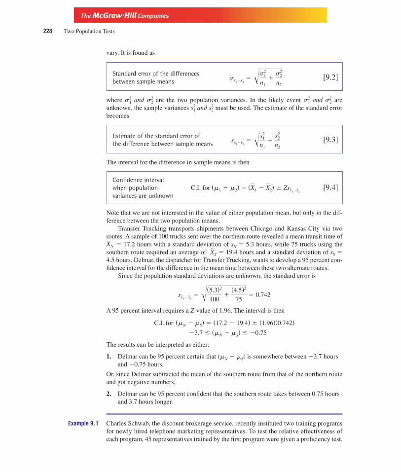
Version, Third Edition
228 Two Population Tests
vary. It is found as
Standard error of the differencesbetween sample means
[9.2]
where and are the two population variances. In the likely event and areunknown, the sample variances and must be used. The estimate of the standard errorbecomes
Estimate of the standard error ofthe difference between sample means
[9.3]
The interval for the difference in sample means is then
Confidence interval when population variances are unknown
[9.4]
Note that we are not interested in the value of either population mean, but only in the dif-ference between the two population means.
Transfer Trucking transports shipments between Chicago and Kansas City via tworoutes. A sample of 100 trucks sent over the northern route revealed a mean transit time of
� 17.2 hours with a standard deviation of sN � 5.3 hours, while 75 trucks using thesouthern route required an average of � 19.4 hours and a standard deviation of sS �4.5 hours. Delmar, the dispatcher for Transfer Trucking, wants to develop a 95 percent con-fidence interval for the difference in the mean time between these two alternate routes.
Since the population standard deviations are unknown, the standard error is
A 95 percent interval requires a Z-value of 1.96. The interval is then
The results can be interpreted as either:
1. Delmar can be 95 percent certain that (mN � mS) is somewhere between �3.7 hoursand �0.75 hours.
Or, since Delmar subtracted the mean of the southern route from that of the northern routeand got negative numbers,
2. Delmar can be 95 percent confident that the southern route takes between 0.75 hoursand 3.7 hours longer.
Example 9.1 Charles Schwab, the discount brokerage service, recently instituted two training programsfor newly hired telephone marketing representatives. To test the relative effectiveness ofeach program, 45 representatives trained by the first program were given a proficiency test.
�3.7 (mN � mS) �0.75
C.I. for (mN � mS) � (17.2 � 19.4) � (1.96)(0.742)
sxN�xS� �(5.3)2
100�
(4.5)2
75� 0.742
XS
XN
C.I. for (m1 � m2) � (X1 � X2) � Zsx1�x2
sx1�x2� �s2
1
n1
�s2
2
n2
s22s2
1
s22s2
1s22s2
1
sx1�x2� �s2
1
n1
�s2
2
n2

Version, Third Edition
Chapter Nine 229
The mean score was � 76.00 points with s1 � 13.50 points. The 40 people trainedunder the second program reported a mean score of � 77.97 and s2 � 9.05. Manage-ment wants to know if one training program is more effective than the other. As the one se-lected to make this determination, you decide to construct a 99 percent confidence intervalfor the difference between the mean proficiency scores of the employees trained under eachprogram. You are also charged with the responsibility of recommending which trainingprogram the company should use exclusively.
Solution: The standard error of the difference between sample means is
The 99 percent interval is found as
Interpretation: You can be 99 percent certain that (m1 � m2) is between �8.34 points and 4.40 points. Ex-pressed differently, you can report with 99 percent confidence that the mean scores of thosetrained by program 2 is between 4.40 points less and 8.34 points more than those trainedby program 1. Of importance, since the interval contains zero, you can be 99 percent con-fident that there is no difference in the mean scores. You may conclude that either programcan be used to train all newly hired representatives.
1. Clark Insurance sells policies to residents throughout the Chicago area. The owner wants to es-timate the difference in the mean claims between people living in urban areas and those resid-ing in the suburbs. Of the 180 urban policies selected for the sample, a mean claim of $2,025was reported, with a standard deviation of $918. The 200 suburban policies revealed a meanclaim of $1,802 and s � $512. What does a 95 percent interval tell the owner about the meanclaims filed by these two groups?
2. Two production processes are used to produce steel pipe. A sample of 100 pipes taken from thefirst production process has a mean length of 27.3 inches and s � 10.3 inches. The correspond-ing figures for 100 pipes produced by the second method are 30.1 and 5.2. What does a 99 per-cent interval reveal about the difference in the mean lengths of pipe produced by these twomethods?
3. Chapman Industries uses two telephone answering devices. Chuck Chapman wishes to deter-mine whether customers who call in are kept waiting longer on the average with one or theother of the systems. If 75 calls on the first system reported a mean wait time of 25.2 sec-onds with s � 4.8 seconds and 70 calls on the second system yielded a mean of 21.3 sec-onds with s � 3.8 seconds, what recommendation would you offer Chuck if he wants tominimize wait time based on a 90 percent interval estimate of the difference in mean waittimes?
4. Two production designs are used to manufacture a certain product. The mean time requiredto produce the product using the old design was 3.51 days with s � 0.79 days. The newdesign required an average of 3.32 days with s � 0.73 days. Equal size samples of 150were used for both designs. What would a 99 percent interval estimate of the difference
�8.34 (m1 � m2) 4.40
C.I. for (m1 � m2) � (76.00 � 77.97) � (2.58)(2.47)
sx1�x2� �(13.50)2
45�
(9.05)2
40� 2.47
X2
X1
Section Exercises

Version, Third Edition
230 Two Population Tests
between the mean times required to produce the product reveal about which design shouldbe used?
5. Explain precisely what the standard error of the difference between sample means actuallymeasures.
B. Small Sample Estimation: The t-DistributionIf either sample is small (less than 30), we cannot assume that the distribution of the dif-ferences in sample means ( � ) fits a normal distribution. The normal deviate Z there-fore cannot be used. Instead, if
1. The populations are normally or near-normally distributed, and
2. The population variances are unknown,
we must turn to the t-distribution.To apply the t-distribution properly, we must also determine whether the variances of
the two populations are equal. How can we presume these variances are equal if, as justnoted above, we don’t know what they are? Many assembly line processes use machines tofill product containers such as cans, bottles, and boxes. When the machines are periodicallyadjusted to ensure proper operation, it is assumed that the mean fill level has changed butthe variance in the fill levels before and after adjustment, although unknown, remains un-changed. Other instances also prevail in which the assumption of equal variances is rea-sonable. A method is presented later in this chapter to test for the equality of two variances.For now, let us examine confidence intervals when (1) the variances are assumed equal andwhen (2) the variances cannot be assumed equal.
1. The Assumption of Equal but Unknown Variances If the two population variancesare equal, there is some variance s2 common to both populations. That is, � � s2.However, due to sampling error, if a sample is taken from each population, the two samplevariances will likely differ from each other as well as from the common variance s2. Butsince the populations have a common variance, the data from both samples can be pooledto obtain a single estimate of s2. This is done by computing the weighted average of thetwo sample variances where the weights are the degrees of freedom n � 1 for each sample.This pooled estimate of the common population variance is
Pooled estimate of the variancecommon to both populations
[9.5]
The confidence interval for the difference between the two population means is then foundas a t-test with n1 � n2 � 2 degrees of freedom.
Interval for the differencein population means [9.6]using pooled data
Avending machine in the student cafeteria dispenses drinks into paper cups.Asample of15 cups yields a mean of 15.3 ounces with a variance of 3.5. After adjusting the machine, asample of 10 cups produces an average of 17.1 ounces with a variance of 3.9. If s2 is assumedto be constant before and after the adjustment, construct a 95 percent confidence interval forthe difference in mean fills. Assume the amounts dispensed are normally distributed.
C.I. for (m1 � m2) � (X1 � X2) � t�s2p
n1�
s2p
n2
s2p �
s21(n1 � 1) � s2
2(n2 � 1)n1 � n2 � 2
s2p
s22s2
1
s21 �s 2
2
X2X1

Version, Third Edition
Chapter Nine 231
Then
With a � 0.05 (a 95 percent level of confidence) and n1 � n2 � 2 � 23 d.f., the t-table re-veals a value of 2.069.
Subtracting the mean fill level after adjustment (17.1) from the mean fill level beforeadjustment (15.3) resulted in negative values for both the lower and upper ends of theinterval. That is, the interval does not contain zero. We can therefore be 95 percent confi-dent that the adjustment increased the mean fill level between 0.19 ounce and 3.41 ounces.
Example 9.2 Wage negotiations between your firm and the union representing your workers are about tocollapse. There is considerable disagreement about the mean wage level of workers in theplant in Atlanta and the plant in Newport News, Virginia. Wages were set by the old laboragreement reached three years ago and are based strictly on seniority. Since wages areclosely controlled by the labor contract, it is assumed that the variation in wages is the sameat both plants and that the wages are normally distributed. However, it is felt that there is adifference between the mean wage levels due to differing patterns of seniority between thetwo plants.
Management’s head labor negotiator wants you to develop a 98 percent confidence in-terval for the difference between the mean wage levels. If a difference exists in the means,wage adjustments must be made to bring the lower wages up to the level of the higher ones.Given the data below, what adjustments, if any, are called for?
Solution: Samples of workers taken from each plant reveal the following information.
Atlanta Plant Newport News Plant
nA � 23 nN � 19X�A � $17.53 per hour X�N � $15.50
� 92.10 � 87.10
Then
Given a � 0.02 and d.f. � 23 � 19 � 2 � 40, Table F in Appendix III reveals a t-valueof 2.423.
�5.09 m1 � m2 9.15
� 2.03 � 7.12
C.I. for m1 � m2 � (17.53 � 15.5) � 2.423�89.85
23�
89.85
19
� 89.85
s2p �
92.10(22) � 87.1(18)23 � 19 � 2
s2Ns2
A
� 3.41 m1 � m2 �0.19
� �1.8 � 1.61
C.I. for m1 � m2 � (15.3 � 17.1) � 2.069�3.66
15�
3.66
10
� 3.66
s2p �
3.5(14) � 3.9(9)15 � 10 � 2

Version, Third Edition
232 Two Population Tests
Interpretation: You can be 98 percent confident that the mean wage in Atlanta is between $9.15 more thanNewport News and $5.09 less than Newport News. Since this interval contains $0, the con-clusion that no difference exists is possible. No adjustment is warranted.
2. Unequal Variances If the population variances are unequal or there is no evidence toassume an equality, the procedures described above do not apply directly, because thedistribution of differences between sample means does not fit a t-distribution with n1 �n2 � 2 d.f. In fact, no exact distribution has been found to adequately describe this sam-pling process, and only approximations have been developed. One such approximation hasbeen proposed using the t-statistic with d.f. slightly altered. In the event � the de-grees of freedom can be found as
Degrees of freedom whenpopulation variances are [9.7]not equal
Since d.f. is calculated in this altered manner, the t-statistic is symbolized as t ′. The confi-dence interval is then calculated as
Interval for differencein population means [9.8]
The Wall Street Journal described two training programs used by IBM. Twelve ex-ecutives who were given the first type of training scored a mean of 73.5 on an achieve-ment test. Although the news article did not report the standard deviation for these12 employees, let us assume that the variance in test scores for this group was 100.2. Fif-teen executives to whom the second training program was administered scored an aver-age of 79.8. Assume a variance of 121.3 for this second group. Develop a 95 percentconfidence interval for the difference in the mean scores of all executives entered in theseprograms.
If d.f. is fractional, round down to the next lowest whole integer. Thus, d.f. � 24. A 95 per-cent confidence interval with 24 degrees of freedom calls for a t′-value of 2.064.
�14.66 m1 � m2 2.06
� �6.3 � 8.36
� (73.5 � 79.8) � 2.064�100.2
12�
121.3
15
C.I. for m1 � m2 � (X1 � X2) � t��s21
n1
�s2
2
n2
� 24.55
d.f. �(100.2�12 � 121.3�15)2
(100.2�12)2�11 � (121.3�15)2�14
C.I. for m1 � m2 � (X1 � X2) � t��s21
n1
�s2
2
n2
d.f. �(s2
1�n1 � s22�n2)
2
(s21�n1)
2�(n1 � 1) � (s22�n2)
2�(n2 � 1)
s22,s2
1

Version, Third Edition
Chapter Nine 233
Since the interval contains zero, there is no strong evidence that there exists any dif-ference in the effectiveness of the training programs.
Example 9.3 Acme Ltd. sells two types of rubber baby buggy bumpers. Wear tests for durability re-vealed that 13 of type 1 lasted an average of 11.3 weeks with a standard deviation of3.5 weeks, while 10 of type 2 lasted an average of 7.5 weeks with a standard deviationof 2.7 weeks. Type 1 costs more to manufacture, and the CEO of Acme doesn’t want to useit unless it averages at least eight weeks longer than type 2. The CEO will tolerate a prob-ability of error of only 2 percent. There is no evidence to suggest that variances in wear forthe two products are equal.
Solution:
A 98 percent confidence interval (a � 0.02) with 20 d.f. requires a t ′-value of 2.528.
Interpretation: Acme can be 98 percent confident that type 1 lasts between 0.5 and 7.1 weeks longer thantype 2. Since the required eight-week difference is not in the interval, the CEO can be98 percent confident he does not want to use type 1.
6. What conditions must be present before the t-distribution can be used?
7. Seventeen cans of Croc Aid report a mean of 17.2 ounces with a standard deviation of 3.2 ounces, and 13 cans of Energy Pro produce a mean of 18.1 ounces and s � 2.7 ounces.Assuming equal variances and normal distributions in population weights, what conclusioncan you draw regarding the difference in mean weights based on a 98 percent confidenceinterval?
8. Grow-rite sells commercial fertilizer produced at two plants in Atlanta and Dallas. Recentcustomer complaints suggest that the Atlanta shipments are underweight, compared to theDallas shipments. If 10 boxes from the Atlanta plant average 96.3 pounds with s � 12.5 and15 boxes from the Dallas plant average 101.1 with s � 10.3, does a 99 percent interval sup-port this complaint? Assume equal variances.
9. Opus, Inc. has developed a process to make gold from seawater. Fifteen gallons taken fromthe Pacific Ocean produced a mean of 12.7 ounces of gold per gallon with s � 4.2 ounces,
0.5 m1 � m2 7.1 weeks� 3.8 � 3.3
C.I. for m1 � m2 � (11.3 � 7.5) � 2.528�(3.5)2
13�
(2.7)2
10
� 20.99 � 20
�[(3.5)2�13 � (2.7)2�10]2
[(3.5)2�13]2
12�
[(2.7)2�10]2
9
d.f. �(s2
1�n1 � s22�n2)
2
(s21�n1)
2�(n1 � 1) � (s22�n2)
2�(n2 � 1)
s1 � 3.5 s2 � 2.7
n1 � 13 n2 � 10
X1 � 11.3 X2 � 7.5
Section Exercises

Version, Third Edition
234 Two Population Tests
and 12 gallons of water from the Atlantic Ocean yielded similar figures of 15.9 and 1.7.Based on a 95 percent interval, what is your estimate of the difference in the mean ounces ofgold from these two sources? There is no reason to assume the variances are equal.
10. Ralphie is off to college next fall. He samples apartments in both the north and the south endsof town to see if there is any difference in mean rents. Those in the north report rents of $600,$650, $530, $800, $750, $700, and $750, and those in the south report $500, $450, $800,$650, $500, $500, $450, and $400. If there is no evidence that variances are equal, what doesa 99 percent interval tell Ralphie about the difference in mean rents?
11. Bigelow Products wishes to develop a 95 percent interval for the difference in mean weeklysales in two target markets. A sample of 9 weeks in market 1 produced a mean and standarddeviation, in hundreds of dollars, of 5.72 and 1.008 respectively. Comparable figures for mar-ket 2, based on a sample of 10 weeks, were 8.72 and 1.208. If the assumption of equal vari-ances is made, what results do you report?
12. U.S. Manufacturing purchases raw materials from two suppliers. Management is concernedabout production delays due to failure to receive shipments on time. A sample of 10 ship-ments from supplier A has a mean delivery time of 6.8 days with s � 2.57 days, while 12shipments from supplier B have a mean of 4.08 days and s � 1.93. If the variances cannot beassumed equal, what recommendation would you make based on a 90 percent interval esti-mate of the difference in mean delivery times?
9.3 Interval Estimates with Paired SamplingAlso called matched pairs, paired sampling involves a procedure in which several pairs ofobservations are matched up as closely as possible in terms of relevant characteristics. Thetwo sets of observations are different in only one respect or “treatment.” Any subsequentdifferences in the two groups are attributed to that treatment. The advantages of pairedsampling are that (1) smaller samples can be used, (2) smaller variances are encountered,(3) fewer degrees of freedom are lost in the analysis, and (4) a smaller sampling error re-sults (the variation between observations is reduced since they are matched up as closely aspossible). For these reasons, paired sampling is often preferred if its application is possible.
Paired Samples Matched pairs are two observations that are as similar as possibleto each other. They differ in only one relevant aspect.
Assume a medical researcher wishes to test the effects of new drugs on patients’ bloodpressure levels. Twenty people in one group are paired off as closely as possible with20 people in a second group in terms of weight, age, sex, level of activity, cholesterol, andany other factor that might affect blood pressure. We then have 20 pairs of “identicaltwins.” One group is given one new drug, and the other group receives the other drug. Noone except the researcher knows which group gets which medication. Any subsequent dif-ferences, good or bad, in the twins’ blood pressures is attributed to the drugs, since we have“corrected” for all other relevant factors affecting blood pressure (such as age and sex); thatis, we have matched up pairs of observations (twins) that are identical in terms of theseother relevant factors.
Another method of using paired samples involves the examination of the same obser-vations before and after treatment. A common practice in industry is to test employees be-fore and after a training program. We then have a “before” test score and an “after” testscore for each observation (employee). Any change in the score can be attributed to thetraining. (The researcher should be cautioned that some bias may affect the sampling

Version, Third Edition
Chapter Nine 235
because the employees may resent being tested or may remember their answers from thefirst test and try to be consistent in their responses.)
Paired sampling has certain advantages in that smaller samples will often lead to moreaccurate results; by controlling for the other relevant factors the researcher does not haveto rely on the use of large samples to reduce sampling error.
To illustrate, assume that we have test scores for 10 employees before and after theyare given additional on-the-job training. The scores are shown in Table 9.1.
Table 9.1Before and AfterTest Scores
Score ScoreEmployee before OJT after OJT di d 2
i
1 9.0 9.2 �0.2 0.042 7.3 8.2 �0.9 0.813 6.7 8.5 �1.8 3.244 5.3 4.9 0.4 0.165 8.7 8.9 �0.2 0.046 6.3 5.8 0.5 0.257 7.9 8.2 �0.3 0.098 7.3 7.8 �0.5 0.259 8.0 9.5 �1.5 2.25
10 7.5 8.0 �0.5 0.2574.0 79.0 �5.0 7.38
Let di be the difference between any matched pair. The mean of the differences between allpairs is then
Mean difference in paired observations [9.9]
The standard deviation of these differences is
Standard deviationof the differences in paired observations
[9.10]
Since n � 30 and the standard deviation of the differences in scores, sd, is unknown, useof the t-statistic is required. If n had been greater than 30 or sd was known, the Z-statisticcould have been used. Furthermore, it must be assumed that the d-values are normally dis-tributed. The distribution of the raw scores themselves is immaterial, but the d-values mustbe normal.
� 0.736
� �7.38 � 10(�0.5)2
9
sd � ��d2i � nd2
n � 1
��5.0
10� �0.5
d ��di
n

Version, Third Edition
236 Two Population Tests
Then, for a 90 percent confidence level and n � 1 � 9 degrees of freedom, a confi-dence interval for the mean of the difference in scores before and after training is
Interval for difference inmeans of paired observations
[9.11]
Since we subtracted the after test scores from the before test scores yielding negative val-ues, we can be 90 percent confident that the mean of the after test scores is between0.073 points and 0.927 points higher.
Example 9.4 Vicki Peplow, regional director of Medicare payments for Aetna Insurance in Peoria, Illi-nois, became aware that two different hospitals seemed to charge vastly different amountsfor the same medical procedure. She collected observations of billing costs for 15 identicalprocedures from each hospital, and constructed a 95 percent confidence interval for the dif-ference between the mean costs submitted by each hospital. Paired sampling was used be-cause Vicki corrected for all relevant factors other than cost.
If a difference does exist, Ms. Peplow plans to report this matter to Medicare authori-ties. Should she make such a report?
Hospital 1 Hospital 2 di d 2i
465 512 �47 2,209532 654 �122 14,884426 453 �27 729543 521 22 484587 632 45 2,025537 418 �119 14,161598 587 �11 121698 376 �322 103,684378 529 �151 22,801376 517 �141 19,881524 476 48 2,304387 519 �132 17,424429 587 �158 24,964398 639 �241 58,081412 754 �342 116,964
�1,698 � �di 400,716 � �
Solution: Given the data above, we have
� 122.037
sd � ��d2i � nd 2
n � 1� �400,716 � (15)(113.2)2
15 � 1
d ��di
n�
�1,698
15� �113.2
d 2i
�0.927 md �0.073
� �0.5 � (1.833)0.736
�10
C.I. for md � d � tsd
�n

Version, Third Edition
Chapter Nine 237
Interpretation: Since negative values resulted when the charges of the second hospital were subtractedfrom those of the first hospital, Vicki can be 95 percent certain that the second hospital ischarging somewhere between $45.61 and $180.79 more than the first hospital for the sameservices. A report to the proper Medicare administrators seems in order.
Figure 9.2 will aid in deciding which formula and which approach should be used inconstructing these intervals.
�180.79 m1 � m2 �45.61
� �113.2 � 67.5886
� �113.2 � (2.145)122.037��15
C.I. for m1 � m2 � d � (t) sd��n
(X1 – X2) ± 2sX1 – X2
(use sX1 – X2 if known)
– –
– –
––
(X1 – X2) ± t–– sp
2
n1
sp2
n2+
(X1 – X2) ± t�–– s1
2
n1
s22
n2+
d ± tsd
n–
Large
samples
Independent
sampling
Pairedsampling
Small sampless
12≠ s
22
Small sampless1
2 = s22
Figure 9.2Calculating Intervalsfor the Difference inTwo PopulationMeans
Section Exercises 13. Rankin Associates will accept bids from two construction companies on a remodeling job in itshome office. The decision about which offer to accept depends in part on the mean completiontimes of similar jobs by each company. Data are collected and paired for several remodelingjobs. Based on a 99 percent level of confidence, which company would you recommend?
Company 1 Company 2 Company 1 Company 2
10.0 9.2 12.5 7.212.2 10.0 7.3 8.415.3 9.2 9.4 10.59.6 10.5 8.7 6.28.6 9.5 9.1 8.19.4 8.4
14. On his recent trip to Las Vegas, Lucky Louie played 15 games of blackjack at the GoldenNugget and 15 games at the Flamingo. To compare his mean winnings, Louie subtracted his“take” at the Flamingo from that at the Nugget and found �di � 40 and �di
2 � 415. Using a95 percent confidence interval, where should Louie play most often if he wants to maximizehis mean winnings?
15. The annual marathon run is coming up this weekend. You have recorded your time over thecourse for the past five races using two types of running shoes. Determined to win the race

Version, Third Edition
238 Two Population Tests
this year, you want to estimate the difference in your mean times using these two types offootgear. Subtracting the times you recorded using SpeedBurst Shoes from the times runningin RocketMaster yielded, in minutes, �di � 8 and �di
2 � 24. At the 90 percent level of confi-dence, which shoe, if either, is preferred?
16. As an investment analyst, you must compare the mean returns of two types of bonds yourclient is interested in purchasing. The data below are for 12 bonds of each type. What recom-mendation would you offer based on a 99 percent interval estimate of the difference betweenthe mean returns of each type of bond? Assume the observations are paired.
Bond 1 Bond 2 Bond 1 Bond 2
3.21% 6.39% 6.58% 4.58%6.50 8.69 4.58 4.008.25 7.89 7.80 7.809.32 9.58 4.60 9.885.26 6.57 5.89 6.584.58 7.48 6.66 7.89
17. The monthly starting salaries in thousands of dollars of 12 business graduates from Tech Uare compared to those from State U using the data shown below. Develop and interpret a95 percent interval for the difference in mean starting salaries obtained by subtracting Statesalaries from Tech salaries.
Tech State Tech State
3.7 5.6 2.5 8.83.6 6.8 3.5 9.55.2 8.5 3.9 7.51.2 6.5 8.2 6.51.6 5.5 4.5 4.55.2 4.8 1.2 8.7
18. Using the data from the previous problem, calculate and interpret the 95 percent interval forthe difference in mean salaries obtained by subtracting Tech from State. What differences doyou find?
9.4 Confidence Intervals for the Difference between Two Proportions
Occasions often arise in which we must compare the proportions of two different popula-tions. Firms continually examine the proportion of defective products produced by differ-ent methods. Medical researchers are concerned about the proportion of men who sufferheart attacks as opposed to the percentage of women. In general, many business matters aredetermined by the estimation of the relative proportions of two populations.
The procedure should be familiar to you by now. The standard error of the differencebetween two sample proportions (p1 � p2) is estimated by
Standard error of the difference in two sample proportions
[9.12]sp1�p2� �p1(1 � p1)
n1
�p2(1 � p2)
n2

Version, Third Edition
Chapter Nine 239
The term sp1�p2recognizes that if several pairs of samples were taken from each population,
(p1 � p2) would vary. Formula (9.12) accounts for that variation. The confidence intervalis
Interval for the difference in popu-lation proportions
[9.13]
A firm conducts a study to determine whether absenteeism of day workers is differentfrom those who work the night shift. A comparison is made of 150 workers from each shift.The results show that 37 day workers have been absent at least five times over the pastyear, while 52 night workers have missed at least five times. What does this reveal aboutthe tendency for absenteeism among the workers? Calculate a 90 percent confidence inter-val of the difference in the proportion of workers on the two shifts who missed five timesor more.
Since the proportion of night workers who were absent five times or more (p2) wassubtracted from the proportion of day workers who were absent, the firm can be 90 percentcertain that the proportion of night workers absent five or more times is between 1.3 per-cent and 18.7 percent higher than that for day workers.
Example 9.5 provides another look at an interval estimation of the difference betweenproportions.
Example 9.5 Your firm uses two different machines to cut Spandex costumes worn by performers in IceCapades extravaganzas. Problems have developed in proper fittings, due to the perfor-mance of the machines. As the director of quality control, your job is to estimate the dif-ference in the proportion of defects produced by each machine. Samples of sizes n1 � 120and n2 � 95 were taken: The first machine produced 38 percent defects and the second,43 percent defects. Set alpha at 5 percent. If the evidence suggests that the difference in theproportion of defects exceeds 5 percent, all costumes will be produced on the machine thatseems to have a lower defect rate. What decision will you make?
Solution:
� 0.0677
sp1�p2� �(0.38)(0.62)
120�
(0.43)(0.57)95
�18.7% (p1 � p2) �1.3%
� �0.10 � 0.087
� (0.25 � 0.35) � (1.65)(0.0526)
C.I. for p1 � p2 � ( p1 � p2) � (Z)sp1�p2
� 0.0526
sp1�p2� �(0.25)(0.75)
150�
(0.35)(0.65)150
p1 �37
150� 0.25, p2 �
52
150� 0.35
C.I. for p1 � p2 � ( p1 � p2) � (Z)sp1�p2
Version, Third Edition
240 Two Population Tests
Interpretation: You can be 95 percent certain that the proportion of defects produced by the first machineis somewhere between 18.27 percent lower and 8.27 percent higher than the second ma-chine. Since the interval contains zero, there is no evidence that there is any difference inthe proportion of defects produced by the machines. Your decision is that it makes no dif-ference which machine you use, and you might as well continue to use both.
19. Of 150 men and 130 women, 27 percent and 35 percent respectively stated that they usedcredit cards to purchase Christmas gifts. Calculate and interpret the 99 percent confidence in-terval for the difference in the proportion of men and women who relied on credit.
20. Records show that, of 1000 out-of-state students, 40 percent went home for spring break,while 47 percent of the 900 in-state students did so. What is the 95 percent confidence inter-val for the difference in the proportion of students who went home?
21. Of 50 graduate students, 10 went to a warm climate for spring break, while 24 out of 75 un-dergraduates did so. Construct the 95 percent interval.
9.5 Selecting the Proper Sample SizeIt is often necessary to determine the proper sample size needed to conduct a study. As withsingle populations, the required sample size depends on (1) the variances of the popula-tions, and (2) the desired degree of accuracy. This section examines how to determine theappropriate sample size for studies involving both means and proportions.
A. Sample Size for m1 � m2
The proper sample size is found by Formula (9.14).
Sample size for differencein population means
[9.14]
An economist at the University of Texas at Arlington has been asked by the Texas Eco-nomic Planning Commission to develop a 99 percent confidence interval for the differencebetween the mean length of service by public employees and that of workers in the privatesector. The commission desires an interval width of three years. Pilot samples yieldvariances of 15 and 21, respectively. How large should the samples taken from each popu-lation be?
Since the interval is to be 3 years, the error is one-half of that, or 1.5 years. Then
Thus, 107 employees should be selected from the public sector and 107 should be selectedfrom the private sector in order to make the comparison.
� 106.5, or 107
n �(2.58)2(15 � 21)
(1.5)2
n �Z 2 (s2
1 � s22)
(error)2
� �0.1827 (p1 � p2) 0.0827
� �0.05 � 0.1327
C.I. for p1 � p2 � (0.38 � 0.43) � (1.96)(0.0677)
Section Exercises

Version, Third Edition
Chapter Nine 241
B. Sample Size for p1 � p2
The correct sample size to estimate the difference between two population proportions isfound by Formula (9.15).
Sample size for difference in popu-lation proportions
[9.15]
Wally Simpleton, the leading candidate in the governor’s race, wants to develop a con-fidence interval with a width of 3 percentage points and a 99 percent level of confidence forthe difference between the proportion of men and the proportion of women who favor hiscandidacy. How large should the samples be? A pilot sample for men and women revealedpm � 0.40 and pw � 0.30. If the interval width is 0.03, the error is 0.03�2 � 0.015.
9.6 Tests of Hypotheses about Two Meanswith Independent Sampling
Tests of hypotheses for differences in means follow a procedure much like that for inter-vals, in that sampling is either (1) independent or (2) paired. In this instance, however, un-like the instance of interval estimation, we are not interested in the size of the difference inmeans, but only in whether a difference does or does not exist. A two-tailed test, for exam-ple, would be expressed as
or the equivalent
This section examines tests with independent sampling for both large and small samples.
A. Large Sample TestsThe hypothesis test for the difference in two population means is much like that for a sin-gle population. The same four steps are involved:
1. The hypotheses are stated.
2. A Z-test or a t-test statistic is calculated.
3. A decision rule is formed.
4. The findings and conclusion are offered.
HA: m1 � m2 � 0
Ho: m1 � m2 � 0
HA: m1 � m2
Ho: m1 � m2
� 13,312 men and 13,312 women
n �(2.58)2[(0.4)(0.6) � (0.3)(0.7)]
(0.015)2
n �Z 2 [p1(1 � p1) � p2(1 � p2)]
(error)2

Version, Third Edition
242 Two Population Tests
The Z-test value is
Z-test statistic for large samples
[9.16]
where is the estimate for the standard error of the differences in sample means, just asit was for interval estimation. Of course, if the population variances are known, should be used.
Weaver Ridge Golf Course wants to see whether the mean time men require to play18 holes is different from that required by women. Fifty foursomes of men and 45 ofwomen are timed, yielding
Men Women
� 3.5 hours � 4.9 hourss � 0.9 hours s � 1.5 hours
Recall from our discussion of interval estimates that
Then,
If a � 0.05, the critical Z-value is �1.96 and the decision rule is:
Decision Rule Do not reject if Ztest is between �1.96. Reject if Ztest is less than�1.96 or more than �1.96.
As Figure 9.3 shows, the null is rejected. Since the null of equality is rejected and the evidence suggests that women take longer on the average. Notice also that the p-valueassociated with the test is virtually zero.
Xw Xm,
Ztest �(3.5 � 4.9) � 0
0.257� �5.45
sx1�x2� �(0.9)2
50�
(1.5)2
45� 0.257
XX
sx1�x2
sx1�x2
Ztest �(X1 � X2) � (m1 � m2)
sx1�x2
0– 1.96 1.96– 5.45
mm – mw = 0
Z
(Xm – Xw)– –
H0: mm = mwHA: mm ≠ mw
If the null iscorrect, the normallydistributed differencesin the sample meansare centered at(mw – mm) = 0.
p-value � 0
Figure 9.3Hypothesis Test forthe Equality ofGolfing Times

Version, Third Edition
Chapter Nine 243
0
0.05
– 1.65– 5.45
mm – m
Z
(Xm – Xw)– –
H0: mm � mwHA: mm � mw
Figure 9.4A One-Tailed Testfor Mean GolfTimes
If the golf course had hypothesized that men take less time, (mm � mw), the hypotheseswould be stated as
and a left-tailed test as seen in Figure 9.4 would be conducted. If a � 0.05 is retained, theleft-tailed test calls for a critical Z-value of �1.65. The Ztest value of �5.45 does not changeand again falls in the rejection region.
Example 9.6 In Example 9.1 above, managers at Charles Schwab constructed a 99 percent interval esti-mate of the difference between the mean proficiency levels of two groups of employees.The result was �8.34 (m1 � m2) 4.40. Suppose instead they wanted to test the hy-pothesis that the mean proficiencies were equal.
Solution: The hypotheses are
Given the data from Example 9.1,
If a � 0.01, the decision rule is
Decision Rule Do not reject if Ztest is between �2.58. Reject otherwise.
As the figure shows, since Ztest � 0.79, the null is not rejected. Further, the p-value is foundto be 0.5000 � 0.2852 � 0.2148 � 2 � 0.43.
Ztest �(76 � 77.97) � 0
2.47� 0.79
HA: m1 � m2
Ho: m1 � m2
HA: mm � mw
Ho: mm � mw
0
0.005 0.005
– 2.58 2.58
0.2148
0.79 Z
0.2852

Version, Third Edition
244 Two Population Tests
Interpretation: The evidence suggests that there is no difference in the mean proficiency of the groups ofemployees trained under the two programs. This position is supported by the fact that theinterval calculated in Example 9.1 contained zero, indicating no difference.
The Minitab printout for the Schwab tests is seen in Display 9.1. Click on Stat Basic Statistics 2-sample t. This will give you the results of both the interval estimateand the hypothesis test. Notice the 99 percent confidence interval as well as the t-value andthe p-value.
Display 9.1Two Sample T-Test and Confidence IntervalTwosample T for Prog 1 vs Prog 2
N Mean StDev SE MeanProg 1 45 76.0 13.5 2.0Prog 2 40 77.97 9.05 1.4
99% C.I. for mu Prog 1 � mu Prog 2: ( �8.4, 4.6)T-Test mu Prog 1 = mu Prog 2 (vs not =): T= �0.78 P�0.44 DF� 77
B. Small Sample Tests: The t-DistributionAs was the case with confidence intervals, tests involving small samples depend onwhether the population variances can be assumed equal, thereby permitting pooled data. Ifthe assumption of equal variances is permitted, the t-test becomes
Small sample hypothesis test with pooled data
[9.17]
Return to Example 9.2. A 98 percent interval estimate of the difference in mean wages ofworkers in Atlanta and Newport News was calculated based on
Atlanta Newport News
n � 23 n � 19� $17.53 � $15.50
s2 � 92.10 s2 � 87.10
The interval was �5.09 (m1 � m2) 9.15. If, instead of an interval estimate, we hadwanted to conduct a hypothesis test for equal means, we would have
Applying these data to Formula (9.17), we have
ttest �(17.53 � 15.5) � 0
�89.85
23�
89.85
19
� 0.69
HA: mA � mN
Ho: mA � mN
XX
ttest �(X1 � X2) � (m1 � m2)
�s2p
n1
�s2
p
n2

Version, Third Edition
Chapter Nine 245
Given that alpha is 2 percent and there are 23 � 19 � 2 � 40 degrees of freedom, the crit-ical t-value is �2.423. The null is therefore not rejected. It would appear that there is nodifference in the mean wage. This conclusion is supported by the fact that the interval con-tained zero.
If the assumption of equal variance is not made, we find
Small sample test with unequal variances
[9.18]
The ttest is compared to a critical t-value based on degrees of freedom determined byFormula (9.7). In Example 9.3, a 98 percent interval for the difference in the mean dura-bility of two types of rubber baby buggy bumpers was estimated to be
These results were based on the data
A hypothesis test for equal means would appear as
The ttest is
If a � 0.02 and the degrees of freedom are 20 based on Formula (9.7), the decision rule is
Decision Rule Do not reject if ttest is between �2.528. Reject otherwise.
Since 2.94 2.528, the null of equality is rejected. Given the evidence suggeststhat Type 1 rubber baby buggy bumpers exhibit greater durability. Again, this assertion issupported by the fact that the interval in Example 9.3 did not contain zero.
9.7 Hypotheses Tests with Paired DataPairing samples to conduct a hypothesis test offers the same advantages as it does inthe construction of confidence intervals. Less sampling error is suffered due to the reduc-tion in variation between observations since they are matched up as closely as possible.
X1 X2,
ttest �(11.3 � 7.5) � 0
�(3.5)2
13�
(2.7)2
10
� 2.94
HA: m1 � m2
Ho: m1 � m2
s1 � 3.5 weeks s2 � 2.7 weeks
n1 � 13 n2 � 10
X1 � 11.3 weeks X � 7.5 weeks
0.5 weeks (m1 � m2) 7.1 weeks
ttest �(X1 � X2) � (m1 � m2)
�s21
n1
�s2
2
n2

Version, Third Edition
246 Two Population Tests
The ttest is
Hypothesis test for matched pairs [9.19]
where is the mean of the differences in the paired observations and sd is the standard errorof those differences and is found using Formula (9.10).
In Example 9.4, Vicki Peplow prepared a 95 percent interval estimate of the differencein costs for identical procedures at two hospitals. The result was
based on n � 15, �di � �1,698, and �di2 � 400,716. If Ms. Peplow were to test a hy-
pothesis of equality, she would find
and
Given t.05,14 � �2.145, the decision rule is:
Decision Rule Do not reject if ttest is between �2.145. Reject otherwise.
This results in a rejection of the null.
22. Samples of sizes 50 and 60 reveal means of 512 and 587 and standard deviations of 125 and145, respectively. At the 2 percent level, test the hypothesis that m1 � m2.
23. At the 1 percent level, test for the equality of means if samples of 10 and 8 yield means of 36and 49 and standard deviations of 12 and 18, respectively. Assume that variances are notequal.
24. Answer the previous problem if it is assumed that variances are equal.
25. Matched pairs of sizes 81 yielded a mean of the differences of 36.5 and a standard deviationof the differences of 29.1. Test for the equality of means. Set a � 0.01.
26. Test Ho: m1 m2 if sample sizes of 64 and 81 produce means of 65.2 and 58.6 and standarddeviations of 21.2 and 25.3. Set a � 5%.
27. Test Ho: m1 � m2 if samples of 100 produce means of 2.3 and 3.1 with standard deviations of0.26 and 0.31. Set a � 1%.
28. Paired samples of sizes 25 reported a mean difference of 45.2 and a standard deviation of thedifferences of 21.6. Test for the equality of means at the 5% level.
ttest ��113.2 � 0
122.037
�15
� �3.59
HA: m1 � m2
Ho: m1 � m2
�$180.79 (m1 � m2) �45.61
d
ttest �d � (m1 � m2)
sd
�n
Section Exercises

Version, Third Edition
Chapter Nine 247
9.8 A Test for the Difference between Two ProportionsProblems often arise in the business world requiring the comparison of two different popu-lation proportions: the proportion of defects produced by one method compared to that pro-duced by a second, or the proportion of bad debts in one firm compared to that in another.
The test for proportions is performed as
Test for the differenceof two proportions [9.20]
where p1 and p2 are the proportions of successes in the samples and sp1�p2is the standard
error in those differences. It is calculated with Formula (9.12) we used in the constructionof confidence intervals.
To illustrate, a retailer wants to test the hypothesis that the proportion of his malecustomers who buy on credit equals the proportion of women who use credit. He selects100 male customers and finds that 57 bought on credit while 52 of the 110 women did so.The hypotheses are
At the 1 percent level the decision rule is:
Decision Rule Do not reject if �2.58 Ztest 2.58. Reject otherwise.
Then,
Since Ztest is between �2.58, the null is not rejected. The retailer cannot conclude at the1 percent level that the proportions of men and women who buy on credit differ.
Example 9.7 Johnson Manufacturing has recently suffered an increase in the number of defective units.The production supervisor feels that the night shift produces a higher proportion of de-fects than does the day shift: pN pD. To compare the proportion of defects, a sample of500 units taken from the daytime production reveals 14 defects. A sample of 700 units fromthe night shift has 22 defects. If a larger proportion of defects originates from nighttime
� 0.092
Ztest �(0.57 � 0.473) � 0
1.05
� 1.05
� �(0.57)(0.43)100
�(0.473)(0.527)
110
sp1�p2� �p1(1 � p1)
n1
�p2(1 � p2)
n2
HA: pm � pw
Ho: pm � pw
Ztest �( p1 � p2) � (p1 � p2)
sp1�p2

Version, Third Edition
248 Two Population Tests
production, the supervisor intends to institute a training program for those workers to im-prove their job skills. At the 5 percent level, should such a program be implemented?
Solution: Since it is thought that the night workers suffer a higher proportion of defects, the hy-potheses are
and a right-tailed test is required. The decision rule is:
Decision Rule Do not reject if Ztest 1.65. Reject if Ztest 1.65.
The proportion of defects from the night shift is pN � 22�700 � 0.031 and that of the dayshift is pD � 14�500 � 0.028; then
and
Interpretation: Since Ztest is less than 1.65, the null that �N �D is not rejected. The evidence is not strongenough to conclude that the nighttime defect rate is greater than that of the daytime work-ers. The training program should not be instituted.
29. Samples of sizes 120 and 150 produced proportions of 0.69 and 0.73. Test for the equality ofpopulation proportions at the 5 percent level.
30. Two samples of sizes 500 each are used to test the hypothesis that Ho: m1 m2. The sampleproportions are 14 percent and 11 percent. At the 10 percent level, what is your conclusion?
31. Samples of sizes 200 and 250 reveal sample proportions of 21 percent and 26 percent. Testthe hypothesis that Ho: p1 � p2. Set alpha at 1 percent.
9.9 Comparing the Variance of Two Normal PopulationsSeveral of the statistical tests discussed earlier required the assumption of equal populationvariances. At the time you were asked to blindly accept this equality, with the promise thatat a later time you would be shown how to test for it. That time has come: This sectiondemonstrates how to determine if the assumption of equal variances is reasonable. This testis based on the F-distribution, which was named after Sir Ronald A. Fisher (1890–1962)in 1924.
When comparing the variances of two populations, a sample is taken from each popu-lation. The sample variances serve as estimates of their respective population variances. An
� 0.303
Ztest �(0.031 � 0.028) � 0
0.0099
� 0.0099
sp1�p2� �(0.031)(0.969)
700�
(0.028)(0.972)500
HA: pN pD
Ho: pN pD
Section Exercises

Version, Third Edition
Chapter Nine 249
F-distribution is then formed by the ratio of these two sample variances. The F-ratio is
F-ratio used to compare two population variances
[9.21]
where is the larger of the two sample variances and is the smaller of the two samplevariances.
Assume that the variance of the second sample exceeds that of the first. In that case,the F-ratio is F � � . The more exceeds , the less likely it is that and thelarger will be the F-ratio. Therefore, a large F-value will lead to a rejection of the nullHo: .
Manipulating the F-ratio to ensure that the higher sample variance is placed in the nu-merator will make sure that the F-value will always be greater than 1. Notice from Figure 9.5that the F-distribution is not symmetrical and is bounded by zero on the lower end.
s21 � s2
2
s21 � s2
2s21s2
2s21s2
2
s2ss2
L
F �s2
L
s2s
Figure 9.5The F-Distribution
f (F )
0 F
a/2
Do notreject
Rejectionregion
Since the F-ratio is restricted to always exceed 1, there results only one rejection regionin the right tail. Any rejection region that might have otherwise appeared in the left tail isprohibited. Thus, only one-half as much of the area under the distribution is accessible as arejection region. Therefore, it is necessary to divide the chosen alpha-value by 2 and iden-tify a single rejection region in the right tail with an area equal to a�2 as shown in Figure 9.5.
The a-value When controlling the F -ratio to ensure F 1, we are conducting thetwo-tailed test of the hypothesis Ho: as if it were a one-tailed test. It is there-fore necessary to divide the a-value by 2.
Suppose an alpha-value of 10 percent is originally chosen. Dividing by 2, a�2 � 0.05,requires that we consult that portion of Table G (Appendix III) that pertains to an a of5 percent. Further, the F-distribution carries two degrees of freedom: one for the numera-tor, which is equal to n1 � 1 and one for the denominator, which equals n2 � 1, where n1
and n2 are the sample sizes in the numerator and the denominator respectively. Notationalconvenience allows us to express the critical F-value as
A management consultant wishes to test a hypothesis regarding two population means.However, before doing so, he must decide whether there is evidence to suggest that thepopulation variances are equal. In collecting his data, the consultant finds:
Sample 1 Sample 2
Sample size 10 10Standard deviation 12.2 15.4Variance 148.84 237.16
Fa/2, n1�1, n2�1.
s21 � s2
2

Version, Third Edition
250 Two Population Tests
He wishes to test
Using Formula (9.21), and ensuring the higher variance is in the numerator, he finds
If alpha is set equal to 5 percent, F.05�2,9,9 � 3.72. This is found from Table G (Appendix III)by locating that portion of the table dealing with an alpha of 0.05�2 � 0.025. Move acrossthe top row for 9 degrees of freedom for the numerator and then down the column to 9degrees of freedom for the denominator. There the value 3.72 is found. As shown by Fig-ure 9.6, the decision rule is therefore:
Decision Rule Do not reject if F 3.72. Reject if F 3.72.
Since F � 1.59 � 3.72, the null Ho: is not rejected. The consultant can proceedwith the hypothesis test regarding population means under the assumption that the vari-ances are equal.
s21 � s2
2
� 1.59
�(15.4)2
(12.2)2
F �s2
1
s22
HA: s 21 � s 2
2
Ho: s 21 � s 2
2
Figure 9.6The F-Distributionfor Equality ofVariances
f (F )
F3.72
0.025
Do notreject
Rejectionregion
The alpha of 5% isdivided by 2 to identifythe rejection region
H0: s12 = s2
2
HA: s12 ≠ s2
2
Solved Problems1. The Yuppies’ Work Ethic An April 1991 issue of Fortune carried a story about workaholic
baby boomers, ages 25 to 43, who have corporate managerial jobs. The article compared thework life of these young executives who had placed themselves on the fast corporate trackwith workers who committed less time to their jobs. While those in the success-oriented modeoften reported 70, 80, or even 90 hours on the job each week, about 60 was typical. The datawere gathered from interviews of corporate employees. Letting group 1 be the fast-trackersand group 2 be those who spent less time on the job, assume the interviews revealed the fol-lowing statistics regarding weekly work schedules:
Group 1 Group 2
� 62.5 hours � 39.7 hourss1 � 23.7 hours s2 � 8.9 hoursn1 � 175 n2 � 168
X2X1

Version, Third Edition
Chapter Nine 251
Construct and interpret a 90 percent interval estimate of the difference in mean workhours and test the hypothesis of equal means at the 10 percent level.
Solution: Given
Then,
You can be 90 percent confident that the fast trackers work an average of 19.63 hours to65.67 hours longer.
The hypothesis test is
The decision rule is:
Decision Rule Do not reject if Ztest is between �1.65. Reject otherwise.
Since Ztest � 11.88 1.65, the null is rejected.
2. Inflation and Market Power Many economic studies focus on industries in which a gooddeal of market power is concentrated in the hands of just a few firms. It is feared that power-ful firms in such highly concentrated industries will dominate the market to their own selfishadvantage. Firms in nine concentrated industries were paired with firms in an equal number ofindustries in which economic power was more dispersed. Industries in each group werematched with respect to foreign competition, cost structures, and all other factors that can af-fect industry prices. The average price increases in percentages in each industry are shownhere. Does it appear at the 5 percent level that concentrated industries exhibit more pro-nounced inflationary pressures than do less concentrated industries? Construct the appropriateinterval and test the appropriate hypothesis.
Industry Concentrated Less ConcentratedPairings Industries (%) Industries (%) di (%) d 2
i
1 3.7 3.2 0.5 0.252 4.1 3.7 0.4 0.163 2.1 2.6 �0.5 0.254 �0.9 0.1 �1.0 1.005 4.6 4.1 0.5 0.256 5.2 4.8 0.4 0.167 6.7 5.2 1.5 2.258 3.8 3.9 �0.1 0.019 4.9 4.6 0.3 0.09
4.422.0
Ztest �(62.5 � 39.7) � 0
1.92� 11.88
HA: m1 � m2
Ho: m1 � m2
19.63 (m1 � m2) 65.67
� (62.5 � 39.7) � (1.65)(1.92)
C.I. for (m1 � m2) � (X1 � X2) � Zsx1�x2
� 1.92
sx1�x2� �s2
1
n1
�s2
2
n2
� �(23.7)2
175�
(8.9)2
168

Version, Third Edition
252 Two Population Tests
Solution:
We are 95 percent confident that the mean price increase in less concentrated industriesis 0.658 percent lower to 0.218 percent higher.
The hypothesis test is:
The decision rule is:
Decision Rule Do not reject if ttest is between �1.860. Reject otherwise.
Since 0.935 � 1.860, do not reject the null.
3. Small-Sample t-Tests A drilling company tests two drill bits by sinking wells to a maximumof 112 feet and recording the number of hours the procedure took. The first bit was used in12 cases, resulting in a mean time of � 27.3 hours and s1 � 8.7 hours. Ten wells were dugwith the second bit, producing an � 31.7 hours and s2 � 8.3 hours.
Does it appear that one bit is more effective than the other? Set a � 0.10. No evidencesuggests variances are equal. Respond by constructing the appropriate interval and testing theappropriate hypothesis.
Solution:
� 19
� 19.59
�[(8.7)2�12 � (8.3)2�10]2
[(8.7)2�12]2
11�
[(8.3)2�10]2
9
�174.15
8.89
d.f. �[s2
1�n1 � s22�n2]
2
(s21�n1)
2
(n1 � 1)�
(s22�n2)
2
(n2 � 1)
X2
X1
� 0.935
ttest �d � (m1 � m2)
sd
�n
�0.22 � 0
0.706
�9
HA: m1 � m2
Ho: m1 � m2
�0.218 md 0.658
� 0.22 � (1.860)0.706
�9
C.I. for (m1 � m2) � d � tsd
�n
� 0.706
sd � ��d2i � nd 2
n � 1� �4.42 � 9(0.22)2
8
d ��di
n�
2
9� 0.22

Version, Third Edition
Chapter Nine 253
With d.f. � 19, and a � 0.10, t ′ � 1.729.
We can be 90 percent confident that drill 1 takes between 1.88 hours more and 10.68 hoursless.
The hypothesis test is:
The decision rule is:
Decision Rule Do not reject if ttest is between �1.729. Reject otherwise.
Since ttest � �1.211 �1.729, do not reject the null.All the wells were dug with the same drilling team and in the same soil. If for these
reasons, or any others that might be cited, the drilling company felt drilling times had equalvariances, how would the test differ from part? Equal variances allow the pooling of sampledata.
With degrees of freedom equal to n1 � n2 � 2 � 12 � 10 � 2 � 20, t0.10,20 � 1.725. Then
4. The Credit Crunch A study in Retail Management revealed that 131 of 468 women whomade retail purchases did so using a particular credit card, while 57 of 237 men used the samecard. Is there evidence to suggest a difference in the proportion of women and men who usethat card? Let a � 0.05. Construct the interval and test the hypothesis.
�10.69 (m1 � m2) 1.89
� (27.3 � 31.7) � (1.725)�72.63
12�
72.63
10
C.I. for (m1 � m2) � (X1 � X2) � t�s2p
n1
�s2
p
n2
� 72.63 hours squared
�(8.7)2(12 � 1) � (8.3)2(10 � 1)
12 � 10 � 2
s2p �
s21(n1 � 1) � s2
2(n2 � 1)n1 � n2 � 2
� �1.211
ttest �(27.3 � 31.7) � 0
�(8.7)2
12�
(8.3)2
10
HA: m1 � m2
Ho: m1 � m2
�10.68 (m1 � m2) 1.88
� (27.3 � 31.7) � (1.729)�(8.7)2
12�
(8.3)2
10
C.I. for (m1 � m2) � (X1 � X2) � t��s21
n1
�s2
2
n2

Version, Third Edition
254 Two Population Tests
Solution:
There appears to be no difference in the proportion of men and women who use credit.The hypothesis test is:
The decision rule is:
Decision Rule Do not reject if Ztest is between �1.96. Reject otherwise.
Since Ztest � 1.14, do not reject the null.
List of Formulas[9.1] Confidence interval for the difference
between two population means—large samples
[9.2]Standard error of the differencesbetween sample means
[9.3]Estimate of the standard error of thedifference between sample means
[9.4] Confidence interval when populationvariances are unknown
[9.5]Pooled estimate of the variance common to both populations
[9.6]Interval for the difference in meansusing pooled data
[9.7]Degrees of freedom when populationvariances are not equal
[9.8]Interval for difference in populationmeans
[9.9]Mean difference in paired observations
d ��di
n
(X1 � X2) � t��s21
n1
�s2
2
n2
(s21�n1 � s2
2�n2)2
(s21�n1)
2�(n1 � 1) � (s22�n2)
2�(n2 � 1)
(X1 � X2) � t�s2p
n1
�s2
p
n2
s2p �
s21(n1 � 1) � s2
2(n2 � 1)n1 � n2 � 2
(X1 � X2) � Zsx1�x2
sx1�x2� �s2
1
n1
�s2
2
n2
sx1�x2� �s2
1
n1
�s2
2
n2
(X1 � X2) � Zsx1�x2
Ztest �(0.28 � 0.24) � 0
0.035� 1.14
HA: pw � pm
Ho: pw � pm
� 0.029 (pw � pm) 0.109
C.I. for (pw � pm) � (0.28 � 0.24) � (1.96)(0.035)
� 0.035
� �(0.28)(0.72)468
�(0.24)(0.76)
237
sp1�p2� �p1(1 � p1)
n1
�p2(1 � p2)
n2

Version, Third Edition
Chapter Nine 255
[9.10]Standard deviation of the differences in paired observations
[9.11]Interval for difference in means of paired observations
[9.12]Standard error of the difference intwo sample proportions
[9.13] Interval for the difference inpopulation proportions
[9.14]Sample size for difference in popula-tion means
[9.15]Sample size for difference in popula-tion proportions
[9.16]Hypothesis test for difference in means—large samples
[9.17]Small sample hypothesis test withpooled data
[9.18]Small sample test with unequalvariances
[9.19] Hypothesis test for matched pairs
[9.20]Test for the difference of twoproportions
[9.21]The F-ratio used to compare twopopulation variances
Chapter Exercises32. An accountant for a large corporation in the Midwest must decide whether to select AT&T or
Sprint to handle the firm’s long-distance telephone service. Data collected for many callsusing both services are reported here.
AT&T Sprint
Number of calls 145 102Mean cost $4.07 $3.89Standard deviation $0.97 $0.85
What does a 95 percent interval reveal about the difference in the population means?
33. The Metro Pet Center compares telephone costs using two different billing programs. Underthe first program, Metro found that over 100 weeks the mean bill was $32.40, with s �$15.10. A sample of 150 weeks using the second program yielded a mean of $47.30, with
F �s2
L
s2s
Ztest �( p1 � p2) � (p1 � p2)
sp1�p2
ttest �d � (m1 � m2)
sd
�n
ttest �(X1 � X2) � (m1 � m2)
�s21
n1
�s2
2
n2
ttest �(X1 � X2) � (m1 � m2)
�s2p
n1
�s2
p
n2
Ztest �(X1 � X2) � (m1 � m2)
sx1�x2
Z 2 [p1(1 � p1) � p2(1 � p2)](error)2
Z 2 (s21 � s2
2)(error)2
(p1 � p2) � (Z)sp1�p2
�p1(1 � p1)n1
�p2(1 � p2)
n2
d � tsd
�n
sd � ��d2i � nd2
n � 1

Version, Third Edition
256 Two Population Tests
s � $13.20. Calculate and interpret the 95 percent confidence interval for the difference be-tween the means of the two programs.
34. In an article on business travel, U.S. News & World Report stated that the mean cost for onenational hotel chain was $45.12 per night, and a second chain was $42.62 per night. Assumethese statistics are based on samples of 82 and 97, respectively, and that population vari-ances for each chain are known to be 9.48 and 8.29 dollars squared, respectively. You mustdetermine which chain of hotels your company will use. At the 1 percent level, what doesthe confidence interval indicate your decision should be? Does it make a difference whichyou use?
35. Assume the sample sizes in the previous problem are n1 � 182 and n2 � 197.
a. Without working the problem, explain what would happen to the interval with theselarger samples. Why does it happen?
b. Work the problem with these larger samples and see if you were right.
36. A recent issue of Business Week discussed efforts by a major car company to determinewhether one type of vehicle was withstanding the wear and tear of daily use more than a sec-ond type. A finance major who has just graduated from a local university was hired to deter-mine whether any difference exists in mean life. She collects data on the mean number ofmonths a vehicle is in service before the first major repair is necessary, and finds the follow-ing information: vehicle 1: � 27.3 months, s1 � 7.8 months, and n1 � 82 vehicles; vehicle2: � 33.3 months, s2 � 10.4 months, and n2 � 73 vehicles. At the 2 percent level, con-struct the confidence interval and interpret its results.
37. Professor James wants to estimate the difference in the mean time two organizations requireto decide on grant requests submitted to them. If 14 grant requests to the National ScienceFoundation (NSF) took an average of 45.7 weeks with a standard deviation of 12.6 weeks,and 12 requests to Health and Human Services (HHS) exhibited respective values of 32.9 and16.8 weeks, calculate and interpret the 90 percent confidence interval for the difference be-tween the means. If NSF takes more than five weeks longer than HHS, James plans to submither requests to the latter. Should she do so? Assume that the variances are equal.
38. To compare the means of daily sales revenues, a retailer selects a sample size of 12 weeksfrom one store, with mean revenues of $125.40 and a standard deviation of $34.50, and asample of 15 weeks from another store, with a mean of $117.20 and standard deviation of$21.50. Calculate and interpret the 99 percent confidence interval for the difference betweenthe population means. Set .
39. A management team was asked to solve 10 different quality control problems commonly en-countered in their work. A second management team was asked to solve the same problems.Solution times in minutes required by each team are shown below. Calculate and interpret the90 percent confidence interval for the difference between the population mean times requiredfor the two teams. What can you conclude about the relative problem-solving ability of thetwo teams?
Problem Team 1 Team 2
1 12 252 15 263 14 214 21 235 19 316 12 197 25 358 18 289 17 27
10 20 26
s21 � s2
2
X2
X1

Version, Third Edition
Chapter Nine 257
40. The Wall Street Journal reported that Ford Motor Company became interested in the meansalaries of its executives stationed overseas as opposed to those based stateside. The meansalary for 87 executives posted abroad was $78,010, with a standard deviation of $15,700.The same number of executives placed in domestic service revealed a mean and standarddeviation of $69,410 and $10,012. Develop and interpret the 97 percent interval for meandifferences.
41. Sammy Shopper wishes to compare the costs of 10 different services offered by new car deal-ers in his area. The data are displayed here. Calculate and interpret the 90 percent confidenceinterval for the difference between the population means. If quality of service is the same,which dealer should Sammy use—or does it make a difference?
Service Dealer 1 Dealer 2
1 $54 $362 56 353 59 344 65 395 62 376 43 327 38 318 48 309 46 29
10 59 45
42. The Wall Street Journal reported that concern has been raised regarding the environment inwhich beef cattle are kept prior to slaughter. Supposedly, stress-free surroundings promotegrowth and quality of the meat. A beef grower in northern California even advertises that he“treats his cattle to a spectacular seaside view” before preparing them for the meat counter atthe local grocery store. Assume 50 cattle raised in this vacationlike setting gain an average of112 pounds with s � 32.3 pounds over a given time period. During the same time, 50 cowswith a view of the slaughterhouse gain 105.7 pounds on the average with s � 28.7 pounds.Calculate and interpret the 90 percent interval.
43. Several Christmases ago a portion of Santa Claus’s elves unionized. Since that time Santa haswondered whether there was any difference in mean productivity of unionized elves andnonunionized elves. A sample of 150 unionized elves reported a mean output of 27.3 toys perweek per elf, with a standard deviation of 8.7 toys. A sample of 132 nonunionized elvesrevealed a mean of 29.7 toys per week per elf, with s � 10.7. What does a 90 percent intervaltell Mr. Claus about the difference in mean output?
44. Twenty-six mutual funds, each with $5,000 invested in them, are selected for comparison. Ofthe 26 funds, 12 are income oriented, and yielded a mean return of $1,098,60 (including capi-tal gains), with a standard deviation of $43.20. The remaining funds are growth oriented, andgenerated a mean return of $987.60 (including capital gains), with a standard deviation of$53.40.
a. Calculate and interpret the 80 percent confidence interval for the difference between thepopulation mean returns. There is no reason to believe that the variances are equal.
b. What sample size is necessary to be 95 percent certain that the error does not exceed$10.00?
45. The Baldwin Piano Company has long argued that their method of teaching people to play thepiano is superior to that of its competitors. To estimate any difference in the length of timerequired to learn the basic techniques, as the new staff analyst for Baldwin, you select 100students who used your method and find the mean time was 149 hours with s � 37.7 hours.

Version, Third Edition
258 Two Population Tests
The corresponding statistics for 130 students using the competitor’s method prove to be 186and 42.2.
a. At the 99 percent level of confidence, what can you conclude about the difference in themean learning times? Does it appear that your company offers a better method?
b. What sample size is needed to be 99 percent certain that the error does not exceed 5 hours?
46. While serving as a summer intern for a major insurance company, a management major at thelocal university performed a study to measure the mean life expectancy of alcoholics as op-posed to those who do not drink excessively. The company felt that insurance costs were af-fected by the shorter life span of heavy drinkers.
The mean age at death for 100 alcoholics was found to be 63.7 years with s � 17.7,while 100 moderate and nondrinkers lived an average of 75.2 years with s � 8.7. How wouldyou interpret a 95 percent confidence interval for the difference in the mean life of the twogroups?
47. A pricing experiment was conducted by a national chain of stereo equipment outlets. For oneweekend, the price of their top compact disk players was raised by 4 percent in 35 stores andlowered by a like amount in 35 other randomly selected stores. Changes in sales revenue werenoted in each case. In those stores raising their price, revenues on the CD players increased byan average of $842, with s � $217. The mean increase in revenues in those stores loweringprices was $817, with s � $202. The marketing manager for the firm has always felt that anincrease in price would raise revenues more than would a decrease (a concept economists callelasticity of demand). What does a 99 percent interval tell the manager about the mean in-creases in revenue?
48. A controversial theory in finance holds that stocks traded on the organized exchanges alwaysincrease more on Fridays than on Mondays due to the timing of Treasury auctions. As his se-nior project, a finance major at a large university randomly selects 302 stocks trading on theNew York Stock Exchange on Friday and finds the average price change to be 0.375 point,with a standard deviation of 0.075. The 412 stocks randomly selected on Monday’s tradingyielded a mean price change of �0.25 point, with a standard deviation of 0.05. How wouldyou suggest the finance major interpret the results of a 99 percent interval?
49. You have just graduated from college and been hired as a quality control analyst for ElectricCharlie’s, a large producer of lighting equipment. Currently, Electric Charlie’s uses two meth-ods to produce their Bright-Spot home lighting system. To determine whether one method isbetter, you select 50 systems from each production method. Those from the first method con-tinue providing light for a mean time of 45.5 hours, with s � 12.4 hours. Those producedusing the second method burn for an average of 41.2 hours, with s � 15.3.
a. Calculate and interpret the 95 percent confidence interval for the difference between thepopulation mean service times. Your supervisor wants you to make a recommendation.What will it be?
b. Are your samples large enough to be 90 percent certain that the error does not exceed twohours? How large should the sample be?
50. As a new analyst in the financial analysis division of a Florida-based firm making jet skis, youmust determine whether the firm should concentrate its efforts on supplying customers on theWest Coast or those in Florida. The decision will rest in part on which market is paying thehigher price. The CEO feels that the average price on the West Coast is more than $15 abovewhat the firm can receive from Florida customers. Using these data, interpret for the CEO theresults of a 95 percent interval.
West Coast Orders Florida Orders
Number of orders 37 41Mean price $418.10 $397.20Standard deviation 73.00 62.10

Version, Third Edition
Chapter Nine 259
51. Seven Asian nations reported a mean increase in per capita income over the last year of$121.20, with a standard deviation of $23.30. Nine European countries reported correspond-ing figures of $111.10 and $19.10. Calculate and interpret the 90 percent confidence intervalfor the difference between the population mean increases in income. Can you conclude thatone continent seems to have generated larger increases than the other? It does not appear thatthe standard deviations are equal.
52. Six economists working for the government are asked to predict inflation rates for the upcom-ing year. Eight economists who work for private concerns are given the same task. The sixgovernment economists report rates of 4.2 percent, 5.1 percent, 3.9 percent, 4.7 percent,4.9 percent, and 5.8 percent. The eight privately employed economists forecast rates of5.7 percent, 6.1 percent, 5.2 percent, 4.9 percent, 4.6 percent, 4.5 percent, 5.2 percent, and5.5 percent. What is your estimate of the difference in the mean predictions of the two groupsof economists? Set alpha at 10 percent and assume equal variances.
53. Many economic impact studies have been done to determine the effect of labor unions onwage rates. To address this important issue, an economist examines 10 union shops where amean wage rate of $22.07 and s � $8.12 are found. Twelve nonunion shops reveal a mean of$24.17 and s � $9.07. Use a 99 percent interval to estimate any difference in the mean wagelevels. Should your shop unionize? Assume equal variances.
54. The Wall Street Journal reported that a food distributor in the Midwest examined the effectsof two sales programs on per capita milk consumption. Ten cities were treated to extensiveTV advertising, and the subsequent increase in mean daily consumption of 0.25 gallon and astandard deviation of 0.09 gallon was recorded. Twelve other cities were saturated with news-paper advertisements. There resulted an increase of 0.02 gallon in mean consumption, percapita, with s � 0.02 gallon. If variances are assumed to be equal, how would you interpretthe results of a 90 percent interval?
55. As production director for Maxx Manufacturing, you must decide which of two plants shouldbe given the responsibility of producing the wine corks used by Paul Masson Wineries. Thisdecision is to be based on productivity levels. A sample of 67 days at the Northridge plantproduced a mean of 92.2 thousand corks per day with s � 12.2 thousand. The Southridgeplant produced an average 89.2 thousand with s � 15.4, over 54 days.
a. Test the hypothesis of equality of means at the 10 percent level of significance.b. How large must the samples be to be 90 percent confident that the error does not exceed
5,000 corks?
56. Many corporate finance decisions are based on cash flows. An old machine your firm is cur-rently using generated a mean positive net cash flow of $15.6 thousand with a standard devia-tion of $2.3 thousand over an 18-week period. A new machine used by your competitor re-cently provided respective values of $12.1 and $3.4 thousand over a 13-week period. Test thehypothesis of equality of means at the 2 percent level of significance. Based on this analysis,what would you recommend? Assume .
57. Many European countries use a value-added tax (VAT), which is a tax on the value added to agood at each stage of production. Eight countries using a consumption-type VAT reported amean per capita weekly revenue of $1,142, with s � $312. Ten countries using a gross-income-type VAT reported a mean per capita weekly tax take of $1,372, with s � $502. Ifa � 0.05 and s1 � s2, how would you interpret the results of a hypothesis for m1 � m2?
58. The impact of different pay methods on productivity and workers’ levels of satisfaction hasalways been of interest to labor economists. Fortune reported that a sporting goods companyexperimented with the effects of two methods of payment on employee morale in an Ohioplant. Fourteen workers paid a fixed salary were given a test measuring morale and scored amean of 79.7 with s � 8.2. Twelve workers paid on a commission achieved a mean of 72.7with s � 5.1. Set a � 0.10 and assume s1 � s2. What can be concluded regarding the rela-tive merits of the two pay systems based on the resulting hypothesis test?
s21 � s2
2

Version, Third Edition
260 Two Population Tests
59. The chief financial officer (CFO) for a Fortune 500 firm must decide whether debt financingor equity financing would prove less costly. She examines recent market transactions for firmssimilar to hers and finds that 17 firms using bonds (debt financing) experienced a mean cost of17.3 percent with s � 3.7 percent, and 10 recent stock issues (equity financing) resulted infigures of 22.7 percent and 4.7 percent, respectively. Help her test the appropriate hypothesisat the 5 percent level of significance, if . Does this study provide any evidence as tothe lower-cost method of financing?
60. B. F. Skinner, a noted behavior theorist, espoused the use of positive reinforcement to shapework attitudes. Texaco, Inc., has long used Skinner’s techniques. A sample of 45 employeeswho were treated to this positive treatment averaged a score of 5.5 out of 10 on an attitudetest, with s � 1.2. Sixty employees working in an area not receiving positive reinforcementaveraged 4.8 on the test, with s � 1.9.
a. Calculate and interpret the 98 percent confidence interval for the difference between thepopulation means. Do the results seem to support Skinner’s theories?
b. What are the proper sample sizes if you want to be 95 percent certain the error is less than1 point?
61. A plumbing contractor wishes to estimate the difference in the proportion of construction jobsthat require a second visit to the construction site before the job is completed. The contractorintends to submit his work to that plumbing firm with the lower level of repeated visits. Of50 jobs completed by the Alpha Plumbing Corporation, 39 required a second visit, while theOmega Plumbing Group made a second visit on 67 percent of its 60 jobs. What can you con-clude about the difference in the proportions of jobs requiring a second effort based on a95 percent interval? Which company should the contractor use, or does it make a difference?
62. Two “identical” sets of 50 employees are put through two different training programs andsubsequently given aptitude tests. The mean difference in the scores is 13.5, with a standarddeviation in those differences of 4.3. What would a 95 percent interval conclude about the rel-ative effectiveness of the training programs?
63. Snow White buys her seven dwarfs new shovels for Christmas. The amounts that each dwarfcould dig in the mine with the old shovels and the new shovels are shown here. Test theproper hypothesis at the 10 percent level. Did Snow White’s gift to her seven little buddiesimprove output?
Daily Output in Tons
Dwarf Old Shovels New Shovels
Doc 1.7 1.9Happy 1.4 1.5Grumpy 2.1 2.2Bashful 1.9 2.0Sleepy 2.2 2.2Dopey 1.4 1.5Sneezy 1.9 1.8
64. In finance, an efficient market is defined as one that allocates funds to the most productiveuse. A considerable body of literature exists that is designed to determine whether securitiesmarkets are indeed efficient. Business Week recently surveyed financial analysts. Of 110 ana-lysts who work for private manufacturing firms in the effort to sell their firms’ securities,42 felt markets were efficient, while 31 of 75 analysts who work for brokerage houses who as-sist in these sales agreed that markets were efficient. Test the hypothesis at the 5 percent level;does there appear to be a difference in the proportion of these two types of analysts who ac-cept the concept of market efficiency?
65. Two drugs are to be tested for patients’ adverse reactions. Accura is given to 37 patients andit is found that 25 percent have a reaction. Of the 55 people who receive Tardi, 29 percent
s21 � s2
2

Version, Third Edition
Chapter Nine 261
experience a reaction. Set alpha at 1 percent. What can you conclude from the resultinginterval?
66. Many large companies use assessment centers in the employee selection process. To test thebenefit of these centers, IBM recently compared 100 employees hired through their main as-sessment center with 150 employees hired in a less formal manner. The results showed that55 percent of those in the first group failed to advance to mid-level management within sevenyears of employment, while the corresponding figure for the second group was 60 percent.What can you conclude about the difference in the effectiveness of these two hiring methodsbased on a 98 percent interval?
67. Each strategic business unit (SBU) within a company is responsible for developing its ownstrategy. In that effort, Whirlpool Corporation was one of the first American companies to em-phasize strategic marketing strategy. A common approach was through a consumer survey. IfWhirlpool found that 28 percent of the 70 men who were surveyed stated their approval oftinted appliances, while 34 percent of the 80 women did so, what does a 90 percent intervalreveal about the difference in proportion of men and women who prefer tinted washers anddryers?
68. Of 35 people on one weight-reduction plan, 70 percent reach their goal. A second plan worksfor 65 percent of the 50 people who use it.
a. Does a 99 percent interval indicate a significant difference in the success rate of the plans?b. How large must the samples be to ensure with 99 percent confidence that the error does
not exceed 5 percent?
69. United Airlines finds that one-half of a sample of 150 flights are on time when flying fromeast to west. Of 160 east-bound flights, 72 are on time. Set alpha at 10 percent.
a. What does the resulting interval say about the relative likelihood of arriving on time de-pending on the direction of the flight?
b. Your boss, who is flying on United this week, wants to be 90 percent certain the error inthis estimation does not exceed 10 percent. How large should your samples be?
70. As part of her senior project, a marketing major at North Texas State University in Denton,Texas, surveyed 100 men and 100 women at a local shopping mall regarding their buyinghabits. Of the men, 79 said they had used a credit card to make a purchase over $10 in the pastmonth, while 84 of the women admitted to this type of purchase. The student was attemptingto refute the notion that women are more likely to use credit. At the 5 percent level, did she doso? State and test the appropriate hypotheses.
71. A term paper by a computer science major at Ohio State University, entitled “Your Chip IsAbout to Come In,” examined the quality of computer chips manufactured by two companies.Of 453 chips made by company 1, 54 proved defective. Of 317 made by company 2, 43proved defective. If a � 0.10, is there evidence to suggest that one firm maintains stricterquality control than the other, based on the appropriate hypothesis test?
72. Denny Dimwit, a securities analyst for Your Bottom Dollar, Inc. has always felt that convert-ible bonds are more likely to be overvalued than are income bonds. Of 312 convertible bondsexamined last year, Denny found 202 to be overvalued, while 102 of the 205 income bondsproved to be overvalued. Do these data support Denny’s assumption? Set a � 0.10, and testthe hypothesis.
73. Two production methods are used to assemble compact disk players. The average time re-quired by both methods has been estimated to be about 5.6 minutes. However, studies seem tosuggest that the variances in those times differ. It is important to maintain similar productionschedules in order to coordinate the production schedules. Determine whether the variances inproduction times are dissimilar. Fifteen players produced by the first method report a standarddeviation of 5.4 minutes, and 17 players from the second method report a standard deviationof 4.8 minutes. At the 5 percent level of significance, what do you conclude from the appro-priate hypothesis test?

Version, Third Edition
262 Two Population Tests
74. Data are collected to determine whether there is a difference in the variances of daily revenuesat two stores. Given the data below, what is your conclusion based on a hypothesis test withalpha set at 1 percent?
Store 1 Store 2 Store 1 Store 2
$45.78 $67.89 $12.55 $34.9134.66 76.45 37.77 56.8865.89 87.12 21.87 45.9954.78 98.65 23.4598.66 65.87 56.98
C U R T A I N C A L LThe opening scenario in “Setting theStage” described your job task as an in-ternational analyst: you are to compare
investment opportunities in Europe and Asia. You mustprepare a report to be used by your firm’s directors todecide in which area the majority of investments shouldbe made. The decision will rest on several factors. Yourfirm wishes to concentrate where conditions are most fa-vorable with respect to highest mean (1) rates of return,(2) profit levels, (3) investment levels, (4) economicgrowth rates, and (5) measures of political stability. Themean rates of default on loans and investments are also aconsideration. Estimates of the differences between thesemeans are also critical.
The data shown below are contained in a file calledABROAD on your data disk. They were collected by yourfirm’s Data Analysis Section for quarterly data over thepast 20 quarters. RETE and RETA are the rates of return
in Europe and Asia measured in percentages, respectively.Similarly, INVE and INVA are investments in billions ofdollars, PROE and PROA are profits in billions of dollars,GROE and GROA are economic growth rates in percent-ages. LICE and LICA are area evaluations of political sta-bility measured on a Likert scale from 1 to 10 provided by20 political analysts. Each analyst was asked to rate bothEurope and Asia as to the extent of political stability. Thelower the rating, the less stable foreign governments arejudged to be.
Of 25 recent investments in Europe, two suffered de-faults resulting in a complete loss of all money invested.In Asia, 27 investment projects showed seven defaults.
Provide all necessary statistical analysis and a com-plete discussion of the interpretation and results. Clearlystate your conclusions and recommendation as to the area,Europe or Asia, in which your firm should concentrate itsinvestment activity.
RETE RETA INVE INVA PROE PROA LICE LICA GROE GROA
20 15 250 52 10 3 5 2 9 925 17 240 54 14 6 8 4 8 827 14 210 74 15 5 7 2 9 526 12 195 84 17 2 5 3 12 712 8 174 147 21 5 6 6 15 515 9 154 54 25 4 9 2 14 616 7 214 95 21 7 8 1 17 524 5 187 87 26 8 5 5 14 826 14 165 85 18 9 4 2 12 529 14 240 96 17 5 7 3 11 931 15 287 74 15 4 8 2 15 1114 18 247 35 19 7 5 5 12 1215 5 265 68 14 8 6 4 14 814 8 187 54 15 5 8 1 16 918 7 198 78 18 11 5 2 10 69 12 177 104 12 10 6 5 11 88 14 154 108 21 14 8 6 12 7
15 10 147 147 11 15 4 1 14 1116 11 165 158 10 9 7 4 11 524 11 147 211 9 8 8 5 11 4

Version, Third Edition
Chapter Nine 263
From the Stage to Real LifeA visit to the U.S. Census Bureau (www.census.gov) will help you to become more famil-iar with foreign trade as a component of the U.S. economy. From the Census Bureau HomePage, select “Subjects from A to Z.” Here, move through the index to “foreign trade” andclick on it. Select “Trade Balances with U.S. Trading Partners” under the features list.Next, under the heading, Trade Balances with Partner Countries—Current Year, click on“Try it out.” (An advanced version of Netscape might automatically skip the page with the“Try it out” step.) Then go to the area “Select an item for which you want the tradebalance.”
You will be able to select a particular country from a list and view its monthly dataon exports, imports, and trade balances with the United States Data are for 12 months andannual figures are provided. Pick two each of African, Asian, and European countries.Examine the monthly data for each country. Do the trade balances change frequently frompositive to negative? Note your observations and the annual trade balance for each country.How similar are the U.S. trade balances of the two African countries? The two Asiancountries? The two European countries? Compare the African, Asian, and European tradebalances taking two countries at a time from different areas in each comparison. Are youable to detect any patterns either by the size or the direction of the annual balances?
In this same area on the web site, detailed information about goods traded with eachcountry is also available. Look for the heading, Country Detail, and then click on the mostcurrent year. Here, look up and click on each of the six countries for which you obtainedtrade balance information. Are there notable differences between the countries in the goodsthey trade with the United States?

Version, Third Edition
264
C H A P T E R10Analysis of Variance

Version, Third Edition
265
Analysis of Variance
How and whyANOVA works
The sums ofsquares
Mean sumsof squares
The F-ratio
One-way ANOVA
The purposeof blocking
Sum of squaresof the block
Tests oftwo hypothesis
Two-way ANOVA
When and whyit is used
Latin square designFactorial analysis
The Tukeycriterion
The LSDcriterion
Commonunderscoring
Pairwise comparisons
Interaction
Testing hypothesisfor interaction Sum of squares
of row block
Chapter BlueprintAnalysis of variance is used to test hypotheses about the equality of three or more population means.By comparing sample variances, it is possible to draw some conclusion or inference about the relativesizes of population means.

Version, Third Edition
266 Analysis of Variance
S E T T I N G T H E S T A G EThe June 1997 issue ofU.S. News and World Re-port carried a report by the
Central Intelligence Agency (CIA) detailingthe economic performance of the world’slargest economies in 1995. The Group ofSeven (G-7), called the Summit of the Eightsince Russia’s inclusion, met in Denver in1997 to discuss ways to combat world pover-ty. Interest focused on the changing status ofworld economies and the establishment ofeconomic and political policies that wouldfurther global development.
The table below, compiled by the CIAprior to the G-7 Summit, provides a list ofthe world’s 10 largest economies with realgross domestic product (GDP).
Since there have been several positionchanges among the nations over the pastfew years, discussion in Denver centered onshifts in the world economic order. A ques-tion was raised as to whether there was any“real significant difference in the sizes of theeconomics from top to bottom.” Leaders ofthe G-7 nations felt that levels of inflationand unemployment rates listed in the “Cur-tain Call” at the end of this chapter were ofparticular importance in measuring a na-tion’s economic well-being. The materialpresented in this chapter will prove helpfulin addressing these issues.
10.1 IntroductionIn Chapter 9 we tested hypotheses regarding the equality of two populations means.Unfortunately, these tests were restricted in their application to a comparison of only twopopulations. Many business decisions, however, require the comparison of more than twopopulations. It is here that analysis of variance (ANOVA) proves to be useful.
ANOVA is designed specifically to test if two or more populations have the samemean. Even though the purpose of ANOVA is to test for differences in population means,it involves an examination of the sample variances; hence the term analysis of variance.More specifically, the procedure can be used to determine if a particular “treatment” whenapplied to a population will have a significant impact on its mean. The use of ANOVA orig-inated in the field of agriculture, where the term treatment is used as in treating variousparcels of land with different fertilizers and noting any discrepancies in mean crop yields.Today the word treatment is used quite broadly, to refer to the treatment of customers todifferent advertising displays and noting any subsequent differences in mean purchases,the treatment of three groups of employees to three different types of training programs andobserving any differences that occur in mean levels of productivity, or any situation inwhich a comparison of means is desired.
Consider, as an example, the desire to measure the relative effects of three differenttraining programs on employee output. These different types of training may be (1) self-
GDP GDPRank Country (billions of U.S.$) Rank Country (billions of U.S.$)
1 United States $7,248 6 France $1,1732 China 3,500 7 United Kingdom 1,1383 Japan 2,679 8 Italy 1,0894 Germany 1,452 9 Brazil 9775 India 1,409 10 Russia 796

Version, Third Edition
Chapter Ten 267
taught, (2) computer instructed, or (3) taught by a supervisor. In an ANOVA study, theexperimental units are the objects receiving the treatment. In our training example, theemployees constitute the experimental units. The factor is the force or variable whose im-pact on these experimental units we wish to measure. In this case, “training” is the factorof interest. Finally, the three types of training constitute the treatments, or factor levels, ofthe factor “training.”
The manner in which treatments are selected determines whether we are using a fixed-effects model or a random-effects model. The model described above for the employees’training program is a fixed-effects model. The three training programs were chosen, orfixed, prior to conducting the study. We know which three programs we want to test fromthe outset of the study. The conclusions from the study are applicable only to the threeprograms included in the study.
Fixed-Effects Model Specific treatments are chosen or fixed in advance of the study.
In contrast, suppose Apex Manufacturing had many different training programs, andwanted to know whether training programs in general had different effects on employeeperformance. These three training programs used in the study are seen as only a sample ofall training programs that might be used by the firm. It doesn’t matter which three trainingmethods we use in the study to make the comparison. Any conclusions from the study areseen as applicable to the entire population of all training programs. This procedure wouldproduce a random-effects model.
Random-Effects Model The levels (treatments) used in the study are chosen ran-domly from a population of possible levels.
A thorough study of random-effects models is beyond the scope of this text. Our at-tention in this chapter will focus on fixed-effects models.
Three assumptions are essential for the application of ANOVA:
1. All the populations involved are normal.
2. All the populations have the same variance.
3. The samples are independently chosen.
If the number of treatments is designated as c, the set of hypotheses to test is
The letter c is used for the number of treatments because in an ANOVA table, which wewill devise shortly, each treatment is specified in its own column.
You might argue that it would be possible to test the equality of several means by usingseveral two-sample t-tests as we did in Chapter 9. However, certain complications arisethat render this approach ineffective. For example, if a manufacturer wishes to compare themean daily output for three plants, he might test all three of the following sets of hypotheses:
HA: m1 � m2
H0: m1 � m2
HA: Not all means are equal
H0: m1 � m2 � m3≥ � mc

Version, Third Edition
268 Analysis of Variance
and
and
If the null is not rejected in each of the tests, he might conclude that all three means areequal.
At least two problems emerge with this approach. First, as the number of populations(plants) increases, the number of required tests rises markedly. If there are four plants themanufacturer wants to compare, the number of individual tests doubles from 3 to 4C2 � 6tests. The second problem is perhaps even more disturbing. It arises due to a compoundingof the a-value, which is the probability of a Type I error. If the tests are to be conducted atthe 5 percent level, and if there are three populations requiring three separate hypothesestests, the probability of a Type I error is far in excess of 5 percent. It can be calculated as
While we wanted to test at the 5 percent level, the need to make three tests increased theprobability of the Type I error beyond acceptable limits.
10.2 One-Way ANOVA: Completely Randomized DesignThere are several ways an ANOVA experiment can be designed. Perhaps the most com-mon is the completely randomized design or one-way ANOVA. The term comes from thefact that several subjects or experimental units are randomly assigned to different levels ofa single factor. For example, several employees (the experimental units) may be randomlychosen to participate in different types (the different levels) of a training program (thefactor).
The management director for a large industrial firm wants to determine whether threedifferent training programs have different effects on employees’ productivity levels. Theseprograms are the treatments that ANOVA can evaluate. Fourteen employees are randomlyselected and assigned to one of the three programs. Upon completion of the training, eachemployee is given a test to determine his or her proficiency. Four employees are placed inthe first training program, and five in each of the other two. Each of these three groups istreated as a separate sample. The test scores are shown in Table 10.1, along with a few basiccalculations.
Of the 15 cells in the table, 14 have entries. The last cell in the first treatment is anempty cell. A cell identified as Xij where i is the row and j is the column in which the cell islocated. X32 is the entry in the third row and second column. It is seen to be 81. X51 is theempty cell. The number of rows in each column is indicated by r and the number ofcolumns or treatments is indicated by c. In our present case, r � 5 and c � 3.
As seen in Table 10.1, the mean is calculated for each treatment (column). Since thecolumns are identified by the subscript j, the column mean is represented as Finally, theXj .
� 0.1426
� 1 � (0.95)3
P(Type I) � [1 � (1 � 0.05)(1 � 0.05)(1 � 0.05)]
HA: m2 � m3
H0: m2 � m3
HA: m1 � m3
H0: m1 � m3

Version, Third Edition
Chapter Ten 269
Treatments
Program 1 Program 2 Program 3
85 80 8272 84 8083 81 8580 78 90** 82 88
Columnmeans X3 � 85X2 � 81X1 � 80Xj
Table 10.1Employee TestScores
grand mean is calculated for all n observations.
The grand mean for all observationsin the experiment
[10.1]
ANOVA is based on a comparison of the amount of variation in each of the treatments.If the variation from one treatment to the next is significantly high, it can be concluded thatthe treatments are having dissimilar effects on the populations. In Table 10.1 we can identifythree types, or sources, of variation. Note that the first variation is the sum of the other two.
1. There is variation among the total number of all 14 observations. Not all 14 employ-ees scored the same on the test. This is called the total variation.
2. There is variation between the different treatments (samples). Employees in program1 did not score the same as those in programs 2 or 3. This is called between-samplevariation.
3. There is variation within any one given treatment (sample). Not all employees in thefirst sample, for instance, scored the same. This is called within-sample variation.
It is by comparing these different sources of variation that ANOVA can be used to test forthe equality in means of different populations. Any difference that the treatments may havein employee productivity will be detected by a comparison of these forms of variation.
A. The Principle behind ANOVATo determine whether the different treatments have different effects on their respectivepopulations, a comparison is made between the variation within samples (W/S) and thevariation between samples (B/S). The variation in scores within any given sample can becaused by a variety of factors: native ability of employees in that sample, personal motiva-tion, individual efforts and skill, blind luck, and a host of other random circumstances. Thetreatment itself will not produce any variation in the observations within any sample be-cause all observations in that sample receive the same treatment.
It is a different matter with the variation between samples. The variation in scores be-tween samples (from one sample to the next) can be caused by the same random factors asthe variation within a sample (motivation, skill, luck, etc.), plus any additional influence
� 82.14
X5
�85 � 72 � 83 � ≥ � 90 � 88
14
X5
��Xij
n
X5
Version, Third Edition
270 Analysis of Variance
that the different treatments may have. There can be a treatment effect between samplesbecause each sample gets a different treatment.
Treatment Effect Since different samples get different treatments, variation betweensamples can be caused by the different treatment effects.
If a treatment effect exists, it can then be detected by comparing between-sample andwithin-sample variation. If the variation between samples is significantly greater than thevariation within samples, a strong treatment effect is present. This difference between vari-ation between samples and variation within samples is precisely what ANOVA measures.ANOVA is a ratio of the variation between samples to the variation within samples. If thedifferent treatments are having different effects, the variation between samples will rise,causing the ratio to increase. This ratio is based on the F-ratio introduced in the previoussection.
The F -Ratio as Used in ANOVA The F -ratio is a ratio of the variation between sam-ples to the variation within samples.
Again, the variation between samples can be caused in part by different treatments.Variation within a given sample can be caused only by random factors such as the luck,skill, and motivation of the employees. Such variation is independent of the treatment(since all observations within a sample get the same treatment) and is the result only ofrandomized sampling error within the sample.
The F -Ratio When population means are different, a treatment effect is present, andthe deviations between samples will be large compared with the error deviation withina sample. Thus, the F -value, which is a ratio of the treatment variation to the error vari-ation, will rise.
The total variation is equal to the variation caused by the different treatments plus thevariation caused by the random error elements within treatments such as skill, luck, andmotivation. That is,
B. The Sums of SquaresRecognition of these three sources of variation allows us to partition the sums of squares,a procedure necessary for ANOVA. Each of the three types of variation gives rise to a sumof squares. There is (1) the total sum of squares (SST ), (2) the treatment sum of squares(SSTR), and (3) the error sum of squares (SSE). As you might expect,
This illustrates that SST can be partitioned into its two component parts: SSTR and SSE.
SST � SSTR � SSE
Total variation � Treatment variation � Error variation

Version, Third Edition
Chapter Ten 271
We can use these sums of squares to test the equality of population means. Recall fromChapter 3 that the sample variance is calculated as
The sample variance [10.2]
The numerator is the sum of the squares of the deviations from the mean. In this manner,the sum of squares is used to measure variation. The denominator is the number of degreesof freedom. This equation serves as a pattern that can be applied to the sums of squares inANOVA.
Let Xij be the ith observation in the jth sample. For example, X21 is the second observa-tion in the first sample. In Table 10.1, X21 � 72, X32 � 81, X43 � 90, and so on. Then,
Total sum of squares [10.3]
The grand mean is subtracted from each of the 14 observations. The differences are squaredand summed. As shown by the double summation sign in Formula (10.3), this is doneacross all rows and across all columns. Hereafter, the notation for the summation signs isdropped in the interest of simplicity. Using the data in Table 10.1, we have
It should be noted that SST is merely the variation of the observations around the grand mean.For the treatment sum of squares we have
Treatmentsum of squares [10.4]
The number of observations, or rows, in each treatment, rj , is multiplied by the squared dif-ferences between the mean for each treatment, and the grand mean. The results aresummed for all treatments. Formula (10.4) tells us to multiply the number of rows in thejth column (remember, j denotes a column) by the squared deviation of the mean of thatcolumn from the grand mean. Table 10.1 yields
SSTR reflects the variation in the column means around the grand mean.The error sum of squares is expressed as
Error sum of squares [10.5]SSE � ��(Xij � Xj)2
� 65.7
SSTR � 4(80 � 82.14)2 � 5(81 � 82.14)2 � 5(85 � 82.14)2
Xj ,
SSTR � �rj(Xj � X5)2
� 251.7
�≥ (90 � 82.14)2 � (88 � 82.14)2
� (80 � 82.14)2 � (80 � 82.14)2 � (84 � 82.14)2
SST � (85 � 82.14)2 � (72 � 82.14)2 � (83 � 82.14)2
SST � �r
i�1�
c
j�1
(Xij � X5
)2
s2 ��(Xi � X)2
n � 1

Version, Third Edition
272 Analysis of Variance
The mean of a treatment, is subtracted from each observation in that treatment. Thedifferences are squared and summed. This is done for all treatments, and the results aresummed. Using the data in Table 10.1 again, we have
for the first treatment
for the second treatment
for the third treatment
SSE measures the random variation of the values within a treatment around their own mean.A quick check of all these calculations can be done as
If you trust your arithmetic, you can find SSE as simply
C. The Mean Sums of SquaresAs Formula (10.2) for the variance tells us, after we have obtained the sums of squares,each one is divided by its degrees of freedom. A sum of squares divided by its degrees offreedom results in a mean sum of squares. That is, if we average a sum of squares over itsdegrees of freedom, we get a mean sum of squares.
Recall from Chapter 7 that we defined the degrees of freedom as the total number ofobservations in the data set minus any “constraints” that might apply. A constraint was anyvalue that was computed from the data set.
In that regard, notice that in calculating SST, we used the entire data set of n observa-tions to calculate one value. That one value was the grand mean which represents oneconstraint. Therefore, SST carries n � 1 degrees of freedom.
The calculation of SSTR involved the use of the c � 3 sample means from which thegrand mean can be computed. The sample means are therefore seen as individual datapoints and the grand mean is taken as a constraint. SSTR then has c � 1 degrees of freedom.
Finally, we calculated SSE above by noting the deviation of the n � 14 observationsfrom the c � 3 sample means. Thus, SSE has n � c degrees of freedom.
Note that
Since, as noted above, a sum of squares divided by its degrees of freedom produces a meansum of squares, we find the total mean square, or mean square of the total deviation, MST, as
Total mean squares [10.6]MST �SST
n � 1
n � 1 � c � 1 � n � c
d.f. for SST � d.f. for SSTR � d.f. for SSE
X5
,
SSE � SST � SSTR � 251.7 � 65.7 � 186.0
251.7 � 65.7 � 186.0
SST � SSTR � SSE
� 186.0
� (82 � 85)2 � (80 � 85)2 � (85 � 85)2 � (90 � 85)2 � (88 � 85)2
� (80 � 81)2 � (84 � 81)2 � (81 � 81)2 � (78 � 81)2 � (82 � 81)2
SSE � (85 � 80)2 � (72 � 80)2 � (83 � 80)2 � (80 � 80)2
Xj ,

Version, Third Edition
Chapter Ten 273
the treatment mean square (MSTR) as
Mean square treatment [10.7]
and the error mean square (MSE) as
Mean square error [10.8]
Using our data from Table 10.1, we have
These three mean squares are patterned after Formula (10.2). They are sums of squares di-vided by their degrees of freedom, and as such they are measures of variances. It is the ratioof the last two, MSTR and MSE, that is used as the basis of ANOVA to test the hypothesisregarding the equality of means. As noted above, this ratio fits the F-distribution, and isexpressed as
F-ratio for atest of means
[10.9]
In our present case it becomes
� 1.94
F �32.9
16.9
F �MSTR
MSE
� 16.9
�186.0
14 � 3
MSE �SSE
n � c
� 32.9
�65.7
3 � 1
MSTR �SSTR
c � 1
� 19.4
�251.7
14 � 1
MST �SST
n � 1
MSE �SSE
n � c
MSTR �SSTR
c � 1

Version, Third Edition
274 Analysis of Variance
MSTR measures the variation between treatments. If the treatments are having differ-ent effects, MSTR will reflect this by increasing. The F-ratio itself will then increase. Thus,if the F-ratio becomes “significantly” large because MSTR exceeds MSE by such a greatamount, we must recognize that treatment effects probably exist. It is likely that the differ-ent treatments are having different effects on the means of their respective populations, andthe null hypothesis that m1 � m2 � m3 must be rejected.
The critical value for F that is deemed significantly large can be found in Table G (Ap-pendix III) as before. Assume that the management director wishes to test the followinghypothesis at the 5 percent level:
Since MSTR has c � 1 � 3 � 1 � 2 degrees of freedom and MSE has n � c � 14 � 3 �11 degrees of freedom, the critical F-value is found from the table to be F0.05,2,11 � 3.98.The 2 is listed before the 11 in the statement of the degrees of freedom because MSTR isin the numerator.
HA: Not all means are equal
H0: m1 � m2 � m3
DNR
3.981.94
0.05
Rejectionregion
F
f (F)Figure 10.1The Effects ofTraining
The decision rule, depicted in Figure 10.1, is
Decision Rule Do not reject the null if F 3.98. Reject the null if F 3.98.
Since the F-value was calculated to be 1.94 � 3.98, the director should not reject thenull. She can reject at the 5 percent level the hypothesis that the mean test scores are thesame for all three training programs. There is no significant treatment effect associatedwith any of the programs.
D. An ANOVA TableIt is customary to summarize the ANOVA calculations in a table. The general form of theANOVA table is shown in Table 10.2(A), while Table 10.2(B) contains the specific valuespertaining to the training program example.
Notice that the relevant sources of variation are listed, and the F-value of 1.94 isshown in the extreme right column. Example 10.1 provides a more concise illustrationof ANOVA.

Version, Third Edition
Chapter Ten 275
A. The Generalized ANOVA Table
Sum of Degrees MeanSource of Variation Squares of Freedom Squares F-value
Between samples (treatment) SSTR c � 1 SSTR�(c � 1) MSTR�MSEWithin samples (error) SSE n � c SSE�(n � c)Total variation SST n � 1
B. ANOVA Table for Employee Training Programs
Sum of Degrees MeanSource of Variation Squares of Freedom Squares F-value
Between samples (treatment) 65.7 2 32.9 1.94Within samples (error) 186.0 11 16.9Total variation 251.7 13
H0: m1 � m2 � m3
HA: Not all means are equalDecision Rule: Do not reject if F 3.98. Reject if F 3.98.Conclusion: Since F � 1.94 � 3.98, do not reject the null.
Table 10.2An ANOVA TableSummarizingANOVA Calculations
Example 10.1 Robert Shade is vice president for marketing at First City Bank in Atlanta. Recent promo-tional efforts to attract new depositors include certain games and prizes at the bank’s fourbranch locations. Shade is convinced that different types of promotional prizes wouldappeal to different income groups. People at one income level might prefer gifts, while an-other income group might be more attracted by free trips to favorite vacation spots. Shadedecides to use size of deposits as a proxy measure for income. He wants to determinewhether there is a difference in the mean level of deposits between the four branches. If adifference is found, Shade will offer a variety of promotional prizes.
Solution: Seven deposits are randomly selected from each branch and are displayed here, rounded tothe nearest $100. There are c � 4 treatments (samples) and rj � 7 observations in eachtreatment. The total number of observations is n � rc � 28.
Deposit Branch 1 Branch 2 Branch 3 Branch 4
1 5.1 1.9 3.6 1.32 4.9 1.9 4.2 1.53 5.6 2.1 4.5 0.94 4.8 2.4 4.8 1.05 3.8 2.1 3.9 1.96 5.1 3.1 4.1 1.57 4.8 2.5 5.1 2.1
4.87 2.29 4.31 1.46
Shade wants to test the hypothesis at the 5 percent level that
HA: Not all means are equal
H0: m1 � m2 � m3 � m4
� 3.23
�(5.1 � 4.9 � 5.6 �≥� 2.1)
28
X5
��Xij
n
Xj

Version, Third Edition
276 Analysis of Variance
Using Formulas (10.3) to (10.5), he would have
for the first treatment
for the second treatment
for the third treatment
for the fourth treatment
Formulas (10.7) and (10.8) for the mean squares yield
Then the F-ratio is
Shade must use 3 and 24 degrees of freedom, since d.f. for SSTR � 3 and d.f. forSSE � 24. If he wants an a of 5 percent, he finds from Table G (Appendix III) thatF0.05,3,24 � 3.01. The ANOVA table summarizes these figures as
Sum of Degrees of MeanSource of Variation Squares Freedom Squares F-value
Between samples (treatment) 55.33 3 18.44 78.14Within samples (error) 5.67 24 0.236Total variation 61.00 27
H0: m1 � m2 � m3 � m4
HA: Not all means are equalDecision Rule: Do not reject if F 3.01. Reject if F 3.01.Conclusion: Since F � 78.14 3.01, reject the null.
� 78.14
�18.44
0.236
F �MSTR
MSE
� 0.236
MSE �5.67
24
� 18.44
MSTR �55.33
3
� 5.67
� (1.3 � 1.46)2 � ≥ � (2.1 � 1.46)2
� (3.6 � 4.31)2 � ≥ �(5.1 � 4.31)2
� (1.9 � 2.29)2 � ≥ � (2.5 � 2.29)2
� (5.1 � 4.87)2 � ≥ � (4.8 � 4.87)2
SSE � ��(Xij � Xj)2
� 55.33
� 7(4.31 � 3.23)2 � 7(1.46 � 3.23)2
� 7(4.87 � 3.23)2 � 7(2.29 � 3.23)2
SSTR � � rj(Xj � X5
)2
� 61.00
� ≥ � (2.1 � 3.23)2
� (5.1 � 3.23)2 � (4.9 � 3.23)2 � (5.6 � 3.23)2
SST � ��(Xij � X5
)2

Version, Third Edition
Chapter Ten 277
F
0.05DNR
3.01
f (F)
Interpretation: Since F � 78.14, Shade must reject the null. He can be 95 percent confident that the meandeposits at all the branch banks are not equal. If he feels that different income groups areattracted by different types of promotional games, he should devise alternative schemes foreach branch to entice new depositors.
10.3 Tests for Differences between Individual PairsAs you can see from the discussion above, ANOVA tells us whether all means are equal.However, when the null hypothesis is rejected, ANOVA does not reveal which mean(s) is(are) different from the rest. We must use other statistical tests to make this determination.These tests rely on a pairwise comparison of all possible pairs of means. If the absolutevalue (ignoring signs) of the difference between any two sample means is greater thansome standard, it is seen as a significant difference, and we conclude that the respectivepopulation means are different.
We can determine this standard by a variety of statistical procedures including theTukey’s (Too´ Key) method and the least significant difference (LSD).
A. Test for Balanced DesignsBoth the Tukey method and the first of two LSD methods shown here are used if there is anequal number of observations in each sample. Such ANOVA designs are said to be bal-anced. If the design is unbalanced in that the samples are of different sizes, an alternativeLSD approach (to be illustrated shortly) must be used.
ANOVA Designs In a balanced ANOVA design, each sample has the same number ofobservations. If one or more samples have a different number of observations, the de-sign is said to be unbalanced.
In Example 10.1, Mr. Shade found that not all four of his branch banks had the same de-posit levels. The next logical step is to determine which ones are different. Since there is anequal number of observations in all four samples (r � 7), either the Tukey method or thefirst LSD approach can be used.
The test is demonstrated in the following figure.

Version, Third Edition
278 Analysis of Variance
The Tukey Approach Tukey’s method, developed by J. W. Tukey in 1953, requires the cal-culation of the Tukey criterion, T, as shown in Formula (10.10).
Tukey criterion forpairwise comparisons [10.10]
where q is a studentized range distribution with c and n � c degrees of freedom and � isthe selected alpha value. Recall that c is the number of samples or treatments (columns),and n is the total number of observations in all samples combined. These values are 4 and28 in Shade’s branch banking problem.
Table L (Appendix III) gives the critical values for q with a � 0.01 and a � 0.05. Ifa is set at 0.05, Shade wants the value for q0.05,4,24. From that portion of Table L for valueswith a � 0.05, move across the top row for the first degrees of freedom of 4 and down thatcolumn to the second degrees of freedom of 24. There you will find the value 3.90. Then
This Tukey standard criterion of 0.716 is then compared with the absolute difference be-tween each pairwise comparison of sample means. If any pair of sample means has an ab-solute difference greater than the T-value of 0.716, we can conclude at the 5 percent levelthat their respective population means are not equal. The difference between the samplemeans is too great to conclude that they came from similar populations. There is only a5 percent chance that populations with equal means could yield samples of these sizes withmeans that differ by more than 0.716.
In comparing the absolute values of each pairwise difference in sample means to T �0.716, Shade can be 95 percent confident that only branches 1 and 3 have equal meandeposit levels. All the other differences exceed the T-criterion.
These results can be summarized by common underscoring in which connectinglines are drawn under those means that do not differ significantly. The sample means mustfirst be put into an ordered array, usually from lowest to highest as shown here. Since onlybranches 1 and 3 do not differ significantly, they are the only ones connected by a commonunderscore.
Least Significant Difference The least significant difference approach is quite similar to theTukey method. It compares the LSD criterion to the absolute difference in sample means.
X4
1.46
X2
2.29
X3
4.31
X1
4.87
}X3 � X4} � }4.31 � 1.46} � 2.85 0.716*}X2 � X4} � }2.29 � 1.46} � 0.83 0.716*}X2 � X3} � }2.29 � 4.31} � 2.02 0.716*}X1 � X4} � }4.87 � 1.46} � 3.41 0.716*}X1 � X3} � }4.87 � 4.31} � 0.56 � 0.716
}X1 � X2} � }4.87 � 2.29} � 2.58 0.716*
� 0.716
T � 3.90�0.236
7
T � qa,c,n�c�MSE
r

Version, Third Edition
Chapter Ten 279
If the design is balanced, the LSD criterion is
Least significantdifference [10.11]
Note that in using the LSD approach, F has 1 and n � c degrees of freedom. In Shade’scase this is 1 and n � c � 28 � 4 � 24 degrees of freedom. From the F-table, F0.05,1,24 �4.26. Then
In comparing the LSD of 0.536 with each of the absolute differences figured above,Shade finds that all values, including the last one, suggest different population means. TheLSD approach is more conservative in that, given any set of conditions, the LSD criterionwill be less than the Tukey value.
The extensive mathematic calculations required by ANOVA can be facilitated with theuse of modern software packages. Display 10.1 shows the printout for Example 10.1 inwhich Mr. Shade at First City Bank had to decide whether mean deposits at four branchbanks were the same. The upper portion shows the F-value of 78.09, which is comparableto the 78.14 we calculated by hand. The p-value of 0.000 reveals why we rejected the nullat the 5 percent level.
The bottom portion of the printout provides the common underscoring. In accord withthe Tukey criterion, it can be seen that only branches 1 and 3 overlap.
Display 10.1One-Way Analysis of Variance
Analysis of Variance on C1Source DF SS MS F PC2 3 55.333 18.444 78.09 0.000Error 24 5.669 0.236Total 27 61.001
Individual 95% CIs For MeanBased on Pooled StDev
Level N Mean StDev --+---------+---------+---------+----1 7 4.8714 0.5469 (---*--)2 7 2.2857 0.4259 (--*--)3 7 4.3143 0.5210 (--*--)4 7 1.4571 0.4392 (--*--)
--+---------+---------+---------+----Pooled StDev = 0.4860 1.2 2.4 3.6 4.8MTB
With either method, what may appear to be inconsistencies may arise. Assume for thesake of simplicity that there are only three populations under study, requiring three pair-wise comparisons:
}X1 � X2} }X1 � X3} }X2 � X3}
� 0.536
LSD � �2(0.236)4.26
7
LSD � �2(MSE)Fa,1,n�c
r

Version, Third Edition
280 Analysis of Variance
You may find that 1 does not differ significantly from 2, and that 2 does not differ sig-nificantly from 3, but that 1 does differ significantly from 3. This may seem contradictory.According to the rule of transitivity, if 1 equals 2 and 2 equals 3, then 1 must equal 3. How-ever, pairwise comparisons do not involve equalities. In comparing the three populations,we are merely examining statistical evidence to determine if it is sufficiently strong toreject the null. To conclude that 1 does not differ significantly from 2 simply means that wehave insufficient evidence to conclude that they are different. If we conclude, as we didhere, that 1 does differ from 3, it can be assumed that evidence comparing these two sam-ples was stronger.
B. Tests for Unbalanced DesignsIf the design is unbalanced, the Tukey approach and the LSD method discussed above donot apply. Instead, an alternate LSD approach can be used.
Alternate LSD Approach To compare the jth and k th samples, the equation for LSD be-comes
Least significantdifference forunbalanced design
[10.12]
where rj is the number of observations in the jth sample and rk is the number of observa-tions in the kth sample. The LSD value will be different for each pair of pairwise compar-isons, since the number of observations is not the same in every sample.
Example 10.2 As more Americans seek escape from urban pressures, the burden on our national parks hasshown a marked increase with the rise in weekend campers. Outdoor World recently re-ported that the Yosemite National Park in California’s High Sierras hired an economic con-sultant to study the financial position of the park.
Part of the consultant’s effort required the comparison of park revenues from varioussources, including camping fees, fishing licenses, and boating. Displayed here are the datafor several randomly selected visitors. Determine whether there is a difference in the meanrevenues the park receives from these three activities.
Visitor Camping Fishing Boating
1 $38.00 $30.00 $19.002 32.00 25.00 35.003 35.00 31.00 20.004 36.00 35.00 22.005 38.00 ** 25.006 32.00 ** **
$35.17 $30.25 $24.20
Solution: Assuming a is set at 5 percent, then Fa,c�1,n�c � F0.05,2,12 � 3.89. The ANOVA table wouldappear as
Xj
LSDj, k � �� 1
rj
�1
rk�(MSE)Fa,c�1, n�c
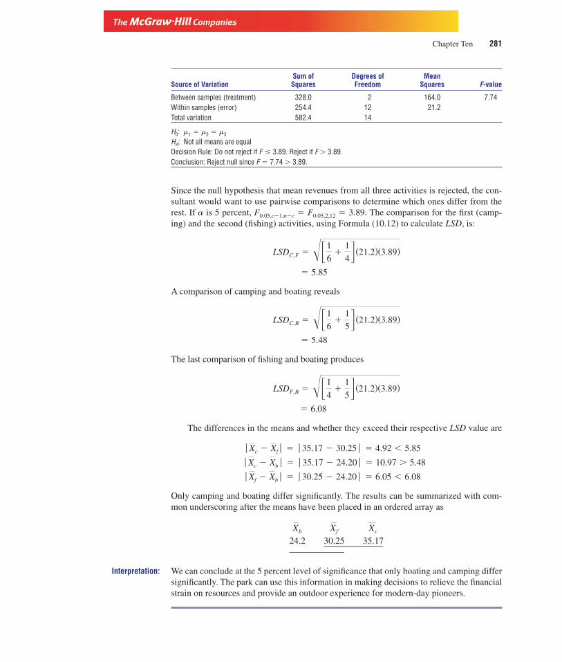
Version, Third Edition
Chapter Ten 281
Sum of Degrees of MeanSource of Variation Squares Freedom Squares F-value
Between samples (treatment) 328.0 2 164.0 7.74Within samples (error) 254.4 12 21.2Total variation 582.4 14
H0: m1 � m2 � m3
HA: Not all means are equalDecision Rule: Do not reject if F 3.89. Reject if F 3.89.Conclusion: Reject null since F � 7.74 3.89.
Since the null hypothesis that mean revenues from all three activities is rejected, the con-sultant would want to use pairwise comparisons to determine which ones differ from therest. If a is 5 percent, F0.05,c�1,n�c � F0.05,2,12 � 3.89. The comparison for the first (camp-ing) and the second (fishing) activities, using Formula (10.12) to calculate LSD, is:
A comparison of camping and boating reveals
The last comparison of fishing and boating produces
The differences in the means and whether they exceed their respective LSD value are
Only camping and boating differ significantly. The results can be summarized with com-mon underscoring after the means have been placed in an ordered array as
Interpretation: We can conclude at the 5 percent level of significance that only boating and camping differsignificantly. The park can use this information in making decisions to relieve the financialstrain on resources and provide an outdoor experience for modern-day pioneers.
Xb
24.2
Xf
30.25
Xc
35.17
}Xf � Xb} � }30.25 � 24.20} � 6.05 � 6.08
}Xc � Xb} � }35.17 � 24.20} � 10.97 5.48
}Xc � Xf} � }35.17 � 30.25} � 4.92 � 5.85
� 6.08
LSDF,B � ��1
4�
1
5�(21.2)(3.89)
� 5.48
LSDC,B � ��1
6�
1
5�(21.2)(3.89)
� 5.85
LSDC,F � ��1
6�
1
4�(21.2)(3.89)

Version, Third Edition
Section Exercises
282 Analysis of Variance
It might seem that the common underscoring in the example is self-contradictory. Itshows that boating and fishing are not different and fishing and camping are not different,yet boating and camping are different. Doesn’t the algebraic rule of transitivity say that ifA equals B and B equals C, then A must equal C? Yes, but we are not dealing with equali-ties in this example. We are simply saying that the difference between boating and fishingis not significant and the difference between fishing and camping is not significant, yet thedifference between boating and camping is large enough to be significant.
1. A producer of house paints wants to compare the brightness factor of his paint using fourdifferent emulsions. Five boards are painted with each type of emulsion and the rating givento each is shown here.
Emulsion
Boards 1 2 3 4
1 79 69 83 752 82 52 79 783 57 62 85 784 79 61 78 735 83 60 75 71
a. At the 1 percent level does it appear that a difference in mean rating exists?b. Use Tukey’s method to test for differences and determine if there is one type the pro-
ducer should use or avoid using. Summarize with common underscoring.
2. A recent study by the American Assembly of Collegiate Schools of Business compared start-ing salaries of new graduates in several fields. A portion of their results is depicted in thetable. At the 5 percent level, does there appear to be a difference in the mean salaries (in thou-sands of dollars) of graduates in different fields? (CIS is computer information systems, andQM is quantitative methods.)
Field of Study
Graduate Finance Marketing CIS QM
1 23.2 22.1 23.3 22.22 24.7 19.2 22.1 22.13 24.2 21.3 23.4 23.24 22.9 19.8 24.2 21.75 25.2 17.2 23.1 20.26 23.7 18.3 22.7 22.77 24.2 17.2 22.8 21.8
3. Considering your results from the previous problem, use Tukey’s method to determine whichmeans are different. Do you get the same results with the LSD approach? Keep a � 0.05.Summarize the results with common underscoring.
4. A medical supply firm wishes to compare the mean daily output of its three plants in Toledo,Ohio; Ottumwa, Iowa; and Crab Apple Cove, Maine. Data were collected for each site andare listed here. At the 10 percent level, is there a difference in the means? The figures are inunits of output.
Toledo: 10, 12, 15, 18, 9, 17, 15, 12, 18
Ottumwa: 15, 17, 18, 12, 13, 11, 12, 11, 12
Crab Apple Cove: 12, 17, 15, 15, 18, 12, 13, 14, 14

Version, Third Edition
Chapter Ten 283
5. Ralph works as a waiter to put himself through taxidermy college. Tips he recently receivedat three restaurants are shown here.
Beef & Boar Sloppy Sam’s Crazy Charlie’s
$5.12 $5.60 $6.006.18 4.25 5.004.25 6.25 2.005.00 7.25 4.506.00 5.00 6.503.25 4.00 5.50
At which place should he work if he wants to maximize his tips, or does it seem to make adifference? Set alpha at 5 percent.
6. Since stockbrokers work for the most part on strict commission, they are interested in tradingactivity on the market. A study was done to determine whether there is a difference in themean commissions paid based on the day of the week, and the data shown here in hundredsof dollars were collected. At the 1 percent level, what days seem to pay the most? UseTukey’s criterion. Summarize with common underscoring.
Monday Tuesday Wednesday Thursday Friday
$21 28 11 15 2526 21 14 14 2324 19 12 12 2632 15 10 12 2825 12 10 16 2426 10 12 13 2524 13 15 18 29
10.4 Two-Way ANOVA: The Randomized Block DesignWith one-way ANOVA, only one factor is thought to influence the experimental units—such as the deposits in the branch banks, or the revenues of the park activities. However,we often find that a second, extraneous influence may impact on the experimental units.For example, our interest may be to compare the mean productivity of three different typesof machines (treatments). However, we realize that in testing these machines, the opera-tors’ skill and experience may affect machine output, causing some confusion about whichmachine is really best. Thus, to get a clear, uncontaminated view of machine capability, wemust in some way eliminate, or correct for, the operators’ influence on final output. This si-multaneous consideration of two forces requires two-way ANOVA.
In order to obtain a decisive measure of machine capability, we must “block” on theextraneous factor by placing the observations in homogeneous groups based on years ofexperience. Thus, the observations are classified by both blocks and treatments. The pur-pose of blocking is to decrease the variation within a treatment (type of machine). This ex-perimental design is called a randomized block design.
If blocking is done effectively and is based on a factor (such as experience) that trulydoes affect productivity, a purer measure of the treatment effect is obtained. However, ifthe factor selected for blocking does not affect productivity (such as a worker’s social se-curity number, hair color, or sex), the results can be quite misleading. It is important to de-termine whether blocking is done correctly, and if the factor upon which blocking is baseddoes have an impact.

Version, Third Edition
284 Analysis of Variance
Systems (Treatments)
Experience Level 1 2 3
1 27 21 25 24.332 31 33 35 33.003 42 39 39 40.004 38 41 37 38.675 45 46 45 45.33
36.5 36.0 36.2
X � 36.27
Xj
Xi
Table 10.3Output Levels forComputer Systems
To illustrate, a large accounting firm is trying to select an office-integrated computersystem from three models currently under consideration. The final choice will depend onthe systems’ productivity. Five operators are selected at random to operate each system. Itis important to realize that the level of experience the employees have in operating com-puters may affect the outcome of the test. There is therefore a need to account for the im-pact of experience in determining the relative merits of the computer systems. The result-ing levels of output measured in units per hour are recorded in Table 10.3. A higher-codedvalue for experience indicates more years of training.
Within any given sample (system) there will occur variation in output due to operatorexperience, proficiency, state of health at the time, and other random error factors. In one-way ANOVA, we identified this as error variation. If any of these random factors associ-ated with the operators materially affect the level of output, the accounting firm must cor-rect for them. The firm may feel that an operator’s years of experience would significantlyaffect his or her productivity. However, the firm is interested in the productivity of thecomputer systems, not that of their employees. It must therefore adjust for employee pro-ductivity by eliminating the effect of operator variability in order to get a more accurate,uncontaminated measure of system quality.
With two-way ANOVA, the total sum of squares is partitioned into three parts: thetreatment sum of squares (SSTR), the error sum of squares (SSE), and the block sum ofsquares (SSBL). Thus,
SST and SSTR are calculated in the same manner as in one-way ANOVA. However, SSE issubdivided into a measure for SSE and SSBL, where
Sum of squaresof the block
[10.13]
The number of treatments in each block, ci, is multiplied by the squared difference be-tween the mean for each block, and the grand mean. The results are then summed for allblocks. The symbol ci is used to indicate the number of treatments in a block (row) becausethe treatments are recorded in columns. From Table 10.3,
The sum of squares of the block measures the degree of variation of the block (row) meansaround the grand mean.
� 765.04
�3(38.67 � 36.27)2 � 3(45.33 � 36.27)2
SSBL � 3(24.33 � 36.27)2 � 3(33 � 36.27)2 � 3(40 � 36.27)2
Xi,
SSBL � �ci(Xi � X5
)2
SST � SSTR � SSE � SSBL

Version, Third Edition
Chapter Ten 285
Formulas (10.3) and (10.4) yield
SSE is calculated as
Error sumof squares
[10.14]
Where there are r blocks and c treatments, there are n � rc observations. The degrees offreedom for each of the sums of squares for the values in Formula (10.14) are
SSE � SST � SSTR � SSBL
(r � 1)(c � 1) � (n � 1) � (c � 1) � (r � 1)
(5 � 1)(3 � 1) � (15 � 1) � (3 � 1) � (5 � 1)8 � 14 � 2 � 4
The mean square total and the mean square treatment are, as before, the sum of theirsquares divided by their degrees of freedom. Thus,
In two-way ANOVA,
Mean square error [10.15]
Mean square block [10.16]
� 191.26
�765.04
4
MSBL �SSBL
r � 1
� 5.1
�40.96
8
MSE �SSE
(r � 1)(c � 1)
� 0.47
�0.93
2
Mean square treatment � MSTR �SSTR
c � 1
� 57.64
�806.93
14
Mean square total � MST �SST
n � 1
� 40.96
� 806.93 � 0.93 � 765.04
SSE � SST � SSTR � SSBL
SST � 806.93 and SSTR � 0.93

Version, Third Edition
286 Analysis of Variance
Sum of Degrees of MeanSource of Variation Squares Freedom Squares F-value
Between samples (treatment) 0.93 2 0.47 0.09Between blocks 765.04 4 191.26 37.50Within samples (error) 40.96 8 5.10Total variation 806.93 14
Table 10.4Two-Way ANOVAfor the ComputerSystems
These calculations are summarized in Table 10.4. The F-values are calculated in the samemanner as in one-way ANOVA:
Notice that two F-values are computed—one using MSTR and one for MSBL. The F-valuefor MSBL is calculated in order to determine whether blocking was done effectively. Recallthat if blocking is based on a factor that does not affect operator productivity, the resultscan be misleading. The accounting firm must therefore test to see whether there is a signif-icant difference between block (row) means. If there is no significant difference betweenmean levels of output based on experience blocks (rows), then experience is not a criticalfactor. In this event, two-way ANOVA should be abandoned, and a return to one-wayANOVA with no distinction between experience levels is called for. At the 5 percent level,the critical F-value for MSBL with 4 and 8 degrees of freedom is found from Table G to beF0.05,4,8 � 3.84. The degrees of freedom of 4 and 8 are used because the F-ratio for blocksuses MSBL with r � 1 � 4 degrees of freedom and MSE with (r � 1)(c � 1) � 8 degreesof freedom.
The accounting firm must first test the hypothesis that the mean level of output foreach experience level is the same. If it is, then experience is not a factor in determining out-put, and blocking on it would prove useless at best. If the mean levels of output of the dif-ferent experience levels are not the same, then the accounting firm must block on experi-ence in order to correct for its impact and thereby obtain a more accurate measure of thedifferences in computer system quality. The hypothesis to test is
where mi are the mean levels of output for each experience (row) level.
Decision Rule Do not reject the null if F 3.84. Reject the null if F 3.84.
HA: Not all row means are equal
H0: m1 � m2 � m3 � m4 � m5
� 37.50
�191.26
5.1
F �MSBL
MSE
� 0.09
�0.47
5.1
F �MSTR
MSE

Version, Third Edition
Chapter Ten 287
Since F � 37.50, the null should be rejected, and the firm should conclude that experiencelevels have an effect on rates of output. It must correct for experience by using two-wayANOVA.
The firm is now ready to test the hypothesis in which it was originally interested. Isthere a difference in the mean output of the computer systems (treatments)? If the a-valueof 5 percent is retained, the Fa,(c�1),(r�1)(c�1) � F0.05,2,8 � 4.46 is found from the table. Thedegrees of freedom of 2 and 8 are used because the F-ratio for the treatments used MSTRwith 2 degrees of freedom and MSE with 8 degrees of freedom. The set of hypotheses is
H0: m1 � m2 � m3
HA: Not all column means are equal
where mi are the column means for the three computer systems.
Decision Rule Do not reject the null if F 4.46. Reject the null if F 4.46.
Table 10.4 reveals that F � 0.09 � 4.46. The null is not rejected, and the firm concludesthat the mean output levels of the three computer systems do not differ once a correctionhas been made for experience. Employees of different experience levels perform equallywell on all machines. It doesn’t matter which computer system they buy.
Example 10.3 provides another illustration of two-way ANOVA.
Example 10.3 A recent issue of Fortune magazine described efforts by a major electronics firm to developa system in which employees would be given the opportunity to evaluate the performanceof their supervisors and other managerial personnel. Assume five employees are selected atrandom and asked to evaluate four of their managers on a scale of 10 to 50. The results,along with row and column means, might appear as in the accompanying table.
Manager (Treatment)
Employee 1 2 3 4
1 31 35 46 38 37.502 29 32 45 36 35.503 13 17 35 20 21.254 28 38 52 39 39.255 14 20 40 20 23.50
23 28.4 43.6 30.6 X � 3.14
The management director for the electronics firm wants to know whether there is a differ-ence in the mean ratings of the four managers.
Solution: The director decides to use two-way ANOVA to test the means.
� 2344.8
� (20 � 31.4)2
� (31 � 31.4)2 � (29 � 31.4)2 � ≥ � (39 � 31.4)2
SST � ��(Xij � X5
)2
Xj
Xi

Version, Third Edition
288 Analysis of Variance
The two-way table becomes
Sum of Degrees of MeanSource of Variation Squares Freedom Squares F-value
Between samples (treatment) 1,145.2 3 381.73 60.79Between blocks 1,124.3 4 281.08 44.76Within samples (errors) 75.3 12 6.28Total variation 2,344.8 19
The director can now determine whether there is a significant difference in the mean rat-ings given by each of the five employees (rows), which would require blocking on the em-ployees. The hypotheses are
H0: m1 � m2 � m3 � m4 � m5
HA: Not all row means are equal
If a � 1 percent is retained, the proper F-value is F0.01,4,12 � 5.41. The F-value associatedwith the test on blocks is shown in the ANOVA table to be 44.76 5.41. The null is re-jected, and the director determines at the 1 percent level of significance that the mean rat-ings by the five employees (rows) are different and blocking is required.
The director can now test his primary hypothesis regarding the mean ratings of thefour managers (columns). The hypotheses are
H0: m1 � m2 � m3 � m4
HA: Not all column means are equal
The F-value of F0.01,3,12 � 5.95 is less than 60.79. The null hypothesis must be rejected atthe 1 percent level of significance.
Interpretation: By including a blocking factor, the director was able to detect a significant difference in themean rating of the managers by the five employees. Without the blocking factor, the varia-tion in the ratings due to the blocks (differences in employee attitudes) would have beenincluded in the error factor SSE. This would have the effect of increasing SSE and MSE.
� 75.3
� 2344.8 � 1145.2 � 1124.3
SSE � SST � SSTR � SSBL
� 1124.3
� 4(23.5 � 31.4)2
� 4(21.25 � 31.4)2 � 4(39 � 31.4)2
� 4(37.5 � 31.4)2 � 4(35.5 � 31.4)2
SSBL � �ci(Xi � X5
)2
� 1145.2
� 5(30.6 � 31.4)2
� 5(23 � 31.4)2 � 5(28.4 � 31.4)2 � 5(43.6 � 31.4)2
SSTR � �rj(Xj � X5
)2

Version, Third Edition
Chapter Ten 289
The F-value would therefore be lower since F � MSTR MSE. As the F-value goes down,there is a greater likelihood of not rejecting the null.
However, with the two-way ANOVA, the MSE is subdivided into variation due toblocks (MSBL) and variation due to error within samples (MSE).
Now that the director knows that not all managers’ ratings are the same, he can useTukey’s method or LSD to determine which are different. In applying these tools to a two-way test, certain changes must be made in the degrees of freedom associated with theTukey method. Rather than explore that involved adjustment, the LSD method as demon-strated earlier can be used with two-way ANOVA.
Display 10.2Two-Way Analysis of Variance
Analysis of Variance for ratingSource DF SS MSEmployee 4 1124.30 281.08Manager 3 1145.20 381.73Error 12 75.30 6.28Total 19 2344.80
Individual 95% CIEmployee Mean ----------+---------+----------+---------+-
1 37.5 (----*---)2 35.5 (---*----)3 21.2 (---*----)4 39.2 (---*----)5 23.5 (---*----)
----------+---------+----------+---------+-24.0 30.0 36.0 42.0
Individual 95% CIManager Mean -+---------+---------+----------+---------+
1 23.0 (---*--)2 28.4 (---*--)3 43.6 (---*--)4 30.6 (---*--)
-+--------+---------+----------+---------+-21.0 28.0 35.0 42.0 49.0
MTB
Display 10.2 shows the Minitab printout for Example 10.3. The top portion providesthe ANOVA table. However, as the Minitab manual notes, you cannot specify whether theeffects are random or fixed with the TWOWAY command. Thus, Minitab does not provideF-values or p-values. Minitab apparently expects you to calculate these by hand. The hy-pothesis for row means (blocking on employees)
H0: m1 � m2 � m3 � m4 � m5
carries an F-value of
MSBL
MSE�
281.08
6.28� 44.76 F0.05,4,12 � 3.49

Version, Third Edition
Section Exercises
290 Analysis of Variance
The null of equal row means is rejected at the 5 percent level, and two-way ANOVA is usedto test the primary hypothesis of equal mean ratings for the managers:
H0: m1 � m2 � m3 � m4
The F-value is
The null of equal mean ratings for the managers is rejected at the 5 percent level. The pair-wise comparisons are shown in the remaining portions of the printout.
The results of the test for row (employee) means are found in the middle section of theprintout. Notice that not all means are equal. The means of employees 3 and 5 are less thanthe other three. The results for the primary hypothesis regarding manager ratings are foundin the last portion of the printout. Manager 3 has the highest rating and manager 1 has thelowest. There does not appear at the 5 percent level of significance to be any difference inthe mean ratings of managers 2 and 4.
7. As a recent graduate with a degree in marketing, you have just landed a big job with a majorcosmetics firm in New York. You must assist in the analysis of the effectiveness of threeadvertising displays. Five consumers are randomly selected. Each is shown an advertisementand asked to rate it. The results are shown here. Your supervisor is unsure how to proceed,but your vast knowledge of statistical analysis based on your college course work tells youthat two-way ANOVA is appropriate since each consumer (block) rated all three displays(treatments). Is there a significant difference in consumers’ attitudes? Set a � 0.01.
Display
Consumer 1 2 3
1 50 45 452 45 30 353 30 25 204 45 35 405 40 30 35
8. Debits and Credits, Inc., an accounting firm in Rocky Top, Tennessee, has a policy of evaluatingeach new employee by having him or her complete several accounting statements and compil-ing any errors. You and two other new members of the firms, Seymore Nueshaum and GretchenNordick, must fill out six statements. They are examined by a senior partner in the firm, andthe errors each of you made are displayed in the table. Does it appear that one of you might beeither more or less efficient in your accounting skills? Set a � 0.05. If so, which one? It isdecided to block on each statement to account for any differences in difficulty that may exist.
Numbers of Errors
Statement You Seymore Gretchen
1 2 2 32 1 3 43 0 1 44 4 6 55 2 3 46 1 4 3
MSTR
MSE�
381.73
6.28� 60.79 F0.05, 3, 12 � 3.26

Version, Third Edition
Chapter Ten 291
9. Current negotiations between union and management focus on the effect on worker output ofmethods of payment. A large firm has five plants. In each one, workers are paid by commis-sion, straight salary, or a bonus plan. Three workers are randomly selected out of all plants,with each paid by a different method. Their daily output measured in units is shown here. It isthought necessary to block on plants, correcting for any differences that might exist in meanplant output.
Based on these data, which payment plan would you suggest to management if theobjective was to maximize output? Set a � 0.05.
Payment Method
Plant Commission Salary Bonus
1 25 25 372 35 25 503 20 22 304 30 20 405 25 25 35
10. A coal company in West Virginia plans to test the mean production of three mines. Fourwork crews will work in each mine and record in tons the resulting output of coal. Sinceeach crew will work in each mine, two-way ANOVA will be used by blocking on crews. Asthe new management supervisor, you must determine if any difference exists in productivityof the mines. Let a � 0.01. Reflect which mines are more productive with commonunderscoring.
Crew Mine 1 Mine 2 Mine 3
1 42.7 54.1 56.92 47.1 59.2 59.23 32.1 53.1 58.74 29.2 41.1 49.2
11. Speedo manufactures touring bikes for the serious rider. The chief quality control engineerdecides to compare the top speeds obtained using three different gearing mechanisms. Fiveexperienced riders are timed using each of the three mechanisms; the results are shown here.Do the data suggest a difference in the average speeds at the 1 percent level?
Mechanism
Rider 1 2 3
1 40 51 372 42 49 383 37 53 384 45 57 415 42 42 40
12. The U-Plant’um Nursery must determine whether there is a difference in the growth rateof saplings that have been treated with different chemical formulas. Since soil condition isa consideration, saplings treated with each formula are planted in each of three types ofsoil. The resulting growth rates over a given period are shown here. Does a differenceappear to exist in the growth factor of the formulas after correcting for soil? Set alpha at1 percent.

Version, Third Edition
292 Analysis of Variance
Formula
Soil Type 1 2 3 4
Sandy 10 8 5 7Clay 12 15 17 14Rocky 17 16 15 15
13. Curly, Moe, and Larry are selling electric forks door to door. Each goes into four neighbor-hoods independently and delivers his own sales pitch. The numbers of forks sold are recordedhere. At the 5 percent level, does it appear one of the salesmen has a brighter future than theothers? If so, which one? Since each salesman called on all neighborhoods, test to seewhether blocking should be used.
Neighborhood Curly Moe Larry
1 15 12 192 27 25 123 24 29 304 32 31 29
14. The National Health Institute surveyed 1,060 adults to determine how they spent their leisuretime. The data have been broken down by age groups and condensed to only 16 observationsfor computational purposes. Does there appear to be any difference in the mean time spentat the different pursuits? The observations are hours per week. Test to determine whetherblocking should be used. Set a � 0.05
Pursuit
Respondents Quality Time(by age) TV Read Sports with Family
15–18 35 12 10 619–25 22 13 12 826–35 25 15 8 15
36 and up 27 20 5 20
10.5 Factorial AnalysisIn our discussion of two-way ANOVA we recognized the presence of a second factor thatwould influence the experimental units. Since we had no interest in analyzing this secondforce, we sought to eliminate its impact. In our earlier example on system productivity, wefeared that experience would contaminate our results of the study, and so we blocked on theexperience level.
Assume now that we want not only to test the computer system, but also to comparethe effect of two different software packages on output. Thus, we wish to test simultane-ously the effect on output of two different factors: computer system and software package.The proper experimental design to employ is called factorial analysis, or two-factorANOVA.
Factorial Analysis Examination of two factors of interest at the same time.
In factorial analysis we can conduct a main-effects test for each factor. Each test is muchlike those presented earlier: they are designed to determine if different levels of either

Version, Third Edition
Chapter Ten 293
factor impact on the experimental units in a different manner. If no main effects are foundfor a factor, the null is not rejected.
Main-Effects Test Tests on both factors to determine whether different levels of thefactor impact on the units differently.
Notice that in factorial analysis there are two factors we wish to consider. Each factor hasmore than one level. We can say that factor A has a levels and factor B has b levels. In ourparticular case we want to compare three computer systems and two software packages.Therefore, factor A has three levels and factor B has two levels. There are a � b, or sixsystem/package combinations. This is referred to as a 3 � 2 factorial design. Each combi-nation is called a treatment. There are now six different treatments under consideration.Each treatment, or system/package combination, is shown in one of the six cells that willappear in the table.
In our earlier studies of ANOVA each cell contained only one observation. For ex-ample, only one person with a given amount of experience recorded his or her output inthe appropriate cell. However, to conduct factorial analysis, more than one observationmust appear in each cell. The number of observations within a cell is often called thenumber of replicates, r. Table 10.5 illustrates. In each of the six cells, the output of sev-eral experimental units (employees) will appear. The first employee working in system 1and package 1 (S1/P1) might produce 27 units of output. If two other employees are cho-sen to work on S1/P1, they might produce 26 and 25 units, respectively. The mean of thatcell, m11, equals 26. The test must be designed so that each cell has the same number ofobservations. An unequal number is beyond the scope of this text. The entire table mightappear as Table 10.5. With three observations in each of the six cells, there are 18 exper-imental units.
FACTOR A(Computer System)
Three Levels of Factor A
1 2 3
27 20 30Factor B 26 22 26(Software 1
25 21 28Package)m11 � 26 m12 � 21 m13 � 28
28 20 30Two Levels of 27 26 31Factor B 2
29 23 29m21 � 28 m22 � 23 m23 � 30
Table 10.5Cell Configurationfor FactorialAnalysis
The design is said to be completely randomized if the 18 units are randomly assignedthree to a cell. On the other hand, assume only three employees are randomly chosen, andeach will perform on all six system/software combinations. In this case the cells would be ho-mogeneous and we would block not only on the columns but also on the rows. This is calleda blocking design in factorial analysis. We will concentrate here on the random configuration.
Factorial analysis has the advantage of being less costly. We can study two factors withone experiment instead of conducting two separate tests. Thus, not only do we save timeand effort, but we achieve the same degree of accuracy using fewer experimental units,since both tests are conducted at the same time.

Version, Third Edition
294 Analysis of Variance
Of perhaps even greater value is the fact that by using a factorial design we can iden-tify any interaction between the two factors that might exist. This interaction would be im-possible to detect if the experiments were conducted separately or if each cell had only oneobservation.
Recall that in factorial analysis, each factor has several levels. Our computer system,factor A, has three levels and the software packages, factor B, have two levels. Interactionis said to exist if one level of factor A works differently (either better or worse) with dif-ferent levels of factor B. For example, computer system 1 might be more (or less) produc-tive with software package 1, while computer system 3 might work better with softwarepackage 2. Thus, the total impact of factor A (system) on productivity depends on whichlevel of factor B (software) is used. The two factors are said to interact in their impact onproductivity.
Interaction The relationship between factor A and the variable under analysis (pro-ductivity in this case) depends on the level of factor B that is used.
Interaction can be detected by examining the mean differences between the levels ofone factor relative to different levels of the other factor. If these mean differences are thesame across all levels of both factors, interaction does not exist. On the other hand, inter-action does exist if the mean differences between levels of one factor are not the same forall levels of the other factor.
Interaction Interaction occurs when the differences in the mean responses for twolevels of one factor are not the same across all levels of the second factor.
This can best be shown by using a system of graphs. Let us begin with a factorial designthat does not exhibit interaction. Consider again the data in Table 10.5. The means of all cellsare shown in Figure 10.2. Notice that the lines do not intersect. Level 2 of the factor packageis higher than level 1 for all three levels of the factor system. In fact, level 2 of package adds2 units over level 1 for all three levels of the factor system. A graph with parallel line seg-ments like these evidences the absence of interaction. We say that the effects are additive.
Figure 10.2Factorial Analysiswithout Interaction
Now assume that the tests produced the results shown in Table 10.6. The graph of thecell means appears in Figure 10.3. Notice now that the lines do cross. There is not a con-stant addition between levels of the package factor across all levels of the system factor.While level 2 of package adds 2 units to level 1 at the first level of system (28 26), this

Version, Third Edition
Chapter Ten 295
FACTOR A(Computer System)
Three Levels of Factor A
1 2 3
28 25 30Factor B 26 23 29(Software 1
24 27 28Package)m11 � 26 m11 � 23 m11 � 29
28 29 28Two Levels of 27 31 27Factor B
229 27 26
m11 � 28 m11 � 29 m11 � 27
Table 10.6Factorial Analysiswith Interaction
pattern does not continue. In fact, package level 1 varied from low to high depending onwhich level of system it was paired with. We could say, for example, that output benefitedfrom the interaction derived from a pairing of system level 3 and package level 2.
As noted earlier, the absence of interaction is evidenced by parallel lines. However, thelines need not be perfectly parallel to conclude interaction is not present. To illustrate,when we test the hypothesis that m � 100, we do not need a sample mean of exactly 100to not reject the null. Values close to 100 are sufficient to not reject. In the same manner,graphs with lines that are approximately parallel offer support for the null.
A more compelling method of detecting interaction relies on tests of hypotheses. Wecan identify three hypotheses that we must test:
H0: The column means are all equal (Main-effects test for the systems factor)
H0: The row means are all equal (Main-effects test for the package factor)
H0: No interaction is present
The alternative hypotheses for each test are stated to the contrary, as is the usual case.As with one-way and two-way ANOVA, we are now ready to partition the sums of
squares and construct the factorial table to test the hypotheses. The necessary calculationsare quite tedious when done by hand; we will rely solely on computer analysis to accom-plish this task.
Given the data in Table 10.5, Minitab is used to generate the factorial table in Dis-play 10.3. The test for interaction is F � 0.00�2.83 � 0 � F0.05,2,12 � 3.89. The hypothe-sis of no interaction is not rejected. The impact of the computer system on productivity
Figure 10.3Factorial AnalysisEvidencingInteraction

Version, Third Edition
296 Analysis of Variance
does not depend on which software program is used. The test for a difference in softwareis F � 18.00�2.83 � 6.36 F0.05,1,12 � 4.75. The null that the row means are equal is re-jected. Finally, the test for a difference in system means is F � 78.00�2.83 � 27.56 F0.05,2,12 � 3.89 and the null is rejected.
Display 10.3Two-Way Analysis of Variance
Analysis of Variance for ProductSource DF SS MSSoftware 1 18.00 18.00System 2 156.00 78.00Interaction 2 0.00 0.00Error 12 34.00 2.83Total 17 208.00
MTB
On the other hand, presume that the test of computer systems and software packagesproduced the data shown in Table 10.6. The resulting Minitab printout, Display 10.4, showsthat interaction is present. The F-value of 14.0�2.40 � 5.60 F0.05,2,12 � 3.89.
Display 10.4Two-Way Analysis of Variance
Analysis of Variance for ProductSource DF SS MSSoftware 1 8.00 8.00System 2 4.00 2.00Interaction 2 28.00 14.00Error 12 30.00 2.50Total 17 70.00
MTB
10.6 Latin Square DesignAnother type of blocking design allows us to block on two extraneous variables at the sametime. Recall our example of computer systems in which we wanted to block on experiencelevel to remove its extraneous influence. Assume now that we also want to correct for thetime of day the work is done, since we know that employees’ productivity varies through-out the day. Some employees are more effective during the morning, others during the af-ternoon, and still others are “night people.” Now we have two variables on which we mustblock. We wish to eliminate the influence of two extraneous elements to capture a moreprecise impression of true system capability. The proper experimental scheme is the Latinsquare design.
One of the blocking variables is assigned to the rows and the second to the columns.The treatments are arranged to occur once in each row and in each column. Therefore, thenumber of rows, the number of columns, and the number of treatments must all be the same.
Latin Square Design Used when we want to block out the extraneous effect of twovariables that might cause equivocal results.

Version, Third Edition
Chapter Ten 297
The Latin square design allows the researcher to gain more information with a smallersample size, since it removes even more of the extraneous variation by blocking on twovariables. Unlike factorial analysis, the Latin square design contains only one element pertreatment per cell.
As just noted, if there are r treatments under examination, we must have r levels foreach of the blocking variables. Hence, we have r � r � r 2 elements, thereby suggestingthe term square. The design is called Latin square because Latin letters such as A, B, andC are used to denote the treatments.
Since there are three computer systems we wish to test, we will now select three em-ployees to work on each system during each of the three time periods. We have three treat-ments (computer systems) and three levels for each block: that is, three levels of experienceand three time periods. We say that we have a 3 � 3 Latin square. The three computer sys-tems (treatments) will be identified as A, B, and C. Each treatment will appear in every rowand every column of the square.
We must now partition the sums of squares among the rows, the columns, and thetreatments. This is accomplished using the following set of formulas. The sum of thesquares of the row block (SSRB) is found as
Sum of squaresof the row block [10.17]
where (Row sum) is the sum of each rowr is the number of treatmentsXi is each of the observations
The sum of the squares of the column block (SSCB) is
Sum of squares ofthe column block [10.18]
where (Col sum) is the sum of each column.The sum of the squares of the treatment (SSTR) is
Treatment sumof squares [10.19]
where (TRTi sum) is the sum of each of the treatments, A, B, and C.The total sum of squares is
Total sumof squares [10.20]
where (Xi)2 is the square of all nine values of output. Last, for the error sum of squares, we have
Sum of thesquared errors
[10.21]SSE � SST � SSTR � SSCB � SSRB
SST � �(Xi)2 �
(�Xi)2
r 2
SSTR ��(TRTi sum)2
r�
(�Xi)2
r 2
SSCB ��(Col sum)2
r�
(�Xi)2
r2
SSRB ��(Row sum)2
r�
(�Xi)2
r2

Version, Third Edition
298 Analysis of Variance
Time
RowEmployee Morning Afternoon Evening Totals
1 B/15 A/18 C/11 442 C/12 B/20 A/9 413 A/17 C/19 B/10 46
Column 44 57 30 131Totals
�A � 44�B � 45�C � 42
Table 10.7Data for a LatinDesign
Assume that the experiment produced the data shown in Table 10.7. The first cell ofB/15 means that the first employee working in the morning produced 15 units of outputon machine B. The upper right cell of C/11 means that the first employee working in theevening produced 11 units of output on machine C.
Source of Sum of Degrees MeanVariation Squares of Freedom Square F-value
Row blocks 4.222 2 2.111 0.3877Column blocks 121.555 2 60.778 11.1621Treatments 1.555 2 0.7775 0.1428Error 10.890 2 5.445Total 138.222
H0: m1 � m2 � m3 The mean outputs of all three computers are equal.F � 0.1428 � F0.05,2,2 � 19; do not reject null.
Table 10.8Latin Square Designfor the ComputerTest
Applying Formulas (10.17) to (10.21), we have
Therefore, SSE � 10.89. The table would appear as Table 10.8.
� 138.222
SST � (15)2 � (12)2 � (17)2 �≥� (10)2 �(131)2
32
� 1.5556
SSTR �(44)2 � (45)2 � (42)2
3�
(131)2
32
� 121.5556
SSCB �(44)2 � (57)2 � (30)2
3�
(131)2
32
� 4.222
SSRB �(44)2 � (41)2 � (46)2
3�
(131)2
32
Setting alpha at 5 percent, the F-value for F0.05,2,2 � 19 0.1428, and we therefore donot reject the null hypothesis that there is no difference in the mean output of the comput-ers after adjusting for employee experience and time of day.

Version, Third Edition
Section Exercises
Chapter Ten 299
15. A producer of metal wires wants to compare the tensile strength of wire made with three dif-ferent chemical mixes: A, B, and C. It is necessary to control for the type of oven used to “fire”the mix, and the temperature at which it was fired. Using the data below, what conclusion canyou reach for the producer? Set alpha at 1 percent.
Temperature
Oven Low Medium High
1 A/40 B/42 C/182 B/70 C/19 A/453 C/20 A/51 B/27
16. As marketing director, you are interested in comparing the revenues of three brands—“good,”“better,” “best”—of electric forks your firm sells. To do so, you want to correct for the area ofthe country in which the store is located, and the type of store at which the sale was made.Your assistant collects the data for monthly sales in hundreds of dollars seen here, but has noidea what to do with them. Conduct the test yourself and inform the assistant of the findings.Set alpha at 1 percent.
Area
Store Northeast Southeast Midwest
Discount Good/4.2 Better/9.0 Best /12.9Convenience Better/7.3 Best /11.1 Good/11.3Mall Best /8.0 Good/9.4 Better/10.7
17. A researcher collects data on faculty salaries to determine whether there is a difference inthe mean incomes of those in business, the social sciences, and the natural sciences. Shemust eliminate the extraneous effects of rank and size of school. Using the information seenhere for salaries in thousands of dollars, what do you suppose are her results? Set alpha at1 percent and interpret.
Size
Rank Small Medium Large
Assistant professor Bus�65 SS/60 NS/78Associate professor SS/72 NS/81 Bus/79Full professor NS/82 Bus/73 SS/79
Solved Problems1. Fleecing the Motorist Consumers’ Research published the results of a survey on U.S. dri-
ving habits. The data contained gasoline taxes per household for all 50 states. Six states arerandomly chosen from the four regions of the country to determine whether there is any dif-ference in the annual mean gasoline tax within the regions. The results follow, rounded to thenearest dollar.

Version, Third Edition
300 Analysis of Variance
Region (treatment)
State North (1) South (2) West (3) Midwest (4)
1 $293 $121 $114 $1362 280 116 176 1643 283 223 224 1174 242 238 183 1535 268 118 159 1526 184 222 149 108
258.3 173.0 167.5 138.3
An economist wanted to test at the 5 percent level the hypothesis that, on the average, resi-dents in all four regions pay the same amount in federal gasoline taxes.
Solution:
SSTR is found as
SSE is
Then,
If a is set at 5 percent, F0.05,3,20 � 3.10 as seen here. The hypothesis is H0: m1 � m2 �m3 � m4.
� 1,775
�35,492
24 � 4
MSE �SSE
n � c
� 16,008
�48,023
4 � 1
MSTR �SSTR
c � 1
� 35,492
� (293 � 258.3)2 � � � � � (108 � 138.3)2
SSE � ��(Xij � Xj)2
� 48,023
� 6(258.3 � 184.3)2 � � � � � 6(138.3 � 184.3)2
SSTR � �rj(Xj � X5)2
� 83,515
� (293 � 184.3)2 � � � � � (108 � 184.3)2
SST � ��(Xij � X5)2
X5
� 184.3
Xj

Version, Third Edition
Chapter Ten 301
The ANOVA table is
Source of Variation SS d.f. MS F-value
Between samples (treatment) 48,023 3 16,008 9.02Within samples (error) 35,492 20 1,775Total variation 83,515 23
H0: m1 � m2 � m3 � m4
HA: Not all means are equalDecision Rule: Do not reject the null if F 3.10. Reject if F 3.10.Conclusion: Reject the null.
It can be concluded at the 5 percent level of significance that the mean tax bite is not the samein all four regions.
2. Who Gets Bitten the Hardest? To formulate an effective tax system, the government mustnow determine which regions pay more and which pay less. Using both Tukey’s method andthe LSD approach, the computations would proceed as shown here.
Solution: It is first necessary to find the absolute differences in the sample means of the taxes paid in eachpair of the four regions.
Tukey’s criterion is
If a is set at 5 percent, q0.05,4,20 � 3.96,
Any absolute difference between the sample means greater than 68.11 is significant andsuggests that their respective populations’ means are different. There is only a 5 percent chance
� 68.11
T � 3.96�1,775
6
T � qa,c,n�c�MSEr
}X3 � X4} � }167.5 � 138.3} � 29.2
}X2 � X4} � }173.0 � 138.3} � 34.7
}X2 � X3} � }173.0 � 167.5} � 5.5
}X1 � X4} � }258.3 � 138.3} � 120.0
}X1 � X3} � }258.3 � 167.5} � 90.8
}X1 � X2} � }258.3 � 173.0} � 85.3

Version, Third Edition
302 Analysis of Variance
that two populations could have the same mean and generate samples of these sizes with meansin excess of 68.11. Comparing 68.11 to the six pairs of sample means above, it can be seen thatpopulation 1 (North) has a mean different from the other three; m1 is assumed to be highersince is significantly higher than the rest.
Using the LSD method, we have
F0.05,1,20 � 4.35. Then
The LSD criterion is compared with the absolute differences in sample means above. Any dif-ferences greater than 50.73 are significant. Again, it is seen that those motorists in the Northendure the heaviest tax burden.
3. Acme, Ltd. As a production supervisor for Acme Ltd., Melvin Moore wishes to compareproduction levels of Acme’s four plants. Data on the weekly levels in tons are collected over agiven seven-week period including the four weeks in August and the first three in September.The results are shown in the table.
Plant (treatment)
Week 1 2 3 4 X�i
1 42.7 38.3 42.9 30.1 38.52 47.3 35.1 38.2 37.5 39.53 57.3 42.7 49.9 47.8 49.44 63.1 58.2 59.3 53.9 58.65 49.2 32.7 45.7 33.8 40.46 51.2 30.1 48.3 38.7 42.17 48.0 31.1 45.2 39.7 41.0
51.3 38.3 47.1 40.2
Melvin conducts a one-way ANOVA and finds a significant difference in mean outputlevels. However, before submitting his report to higher management, Melvin comes to animportant realization: The seven weeks were not picked randomly for each plant. Data forthe same seven weeks were used for all four plants. Perhaps he should block on weeks toeliminate any variation due to the time period. Since the same weeks were recorded for eachplant, blocking on weeks is possible.
Solution: SST and SSTR are calculated in the same fashion as in Solved Problem 1 and are found to be 2,276.1and 761.4, respectively. In addition,
� 1,276.6
� � � � � 4(41 � 44.23)2
� 4(38.5 � 44.23)2 � 4(39.5 � 44.23)2
SSBL � �ci(Xi � X5)2
X5
� 44.23
Xj
� 50.73
LSD � �2(1,775)(4.35)6
LSD � �2(MSE)Fa,1, n�c
r
X1

Version, Third Edition
Chapter Ten 303
These calculations are summarized in the two-way ANOVA table:
Source of Variation SS d.f. MS F-value
Between samples (treatment) 761.4 3 253.8 19.23Between blocks 1,276.6 6 212.8 16.12Within samples (error) 238.1 18 13.2Total variation 2,276.1 27
Melvin must first determine whether blocking on weeks is effective. He sets a at 5 per-cent. The F-value for blocks is MSBL MSE, and since MSBL has r � 1 � 6 d.f. and MSEhas (r �)(c � 1) � 18 d.f., F0.05,6,18 � 2.66 is found to be the critical F-value. SinceF � 16.12 2.66, Melvin concludes that the mean output between weeks is different. Block-ing is therefore necessary to correct for variation from one week to the next. Melvin shouldcontinue with his two-way test.
He can now test the primary hypothesis on mean plant output levels.
H0: m1 � m2 � m3 � m4
HA: Not all means are equal
The F-value for treatments has c � 1 � 3 and (r � 1)(c � 1) � 18 d.f. F0.05,3,18 �3.16 � 19.23. The hypothesis is rejected, and Melvin concludes that there is some difference inplant output levels on the average. He can now use LSD to determine which ones are different.
4. Driving in Circles Circle Trucking Company wishes to determine if the mean drivingtime is the same for three different routes. The traffic director for Circle feels that it isnecessary to correct for weather conditions as well as the proficiency of the drivers. Threelevels of weather conditions are identified: poor, fair, and good. Three drivers with varyingabilities are selected and each covers all three routes under each of the three weatherconditions. The results are reported in the Latin square shown here. Recall that the Latinletters indicate the variables under examination—in this case, routes. Times are recorded inminutes.
� 13.2
�238.1
(7 � 1)(4 � 1)
MSE �SSE
(r � 1)(c � 1)
� 212.8
�1,276.6
7 � 1
MSBL �SSBL
r � 1
� 253.8
�761.4
4 � 1
MSTR �SSTR
c � 1
� 238.1
SSE � SST � SSTR � SSBL

Version, Third Edition
304 Analysis of Variance
Weather
RowDriver Poor Fair Good Totals
1 A/20 C/18 B/17 552 C/22 B/10 A/10 423 B/18 A/9 C/8 35
Column 60 37 35 132Totals
�A � 39 �B � 45 �C � 48
Solution: Using the Latin square design since there are two extraneous variables to correct for (skills andweather), the calculations appear as
Source of Sum of Degrees of MeanVariation Squares Freedom Square F-value
Row blocks(Driver) 686.667 2 34.33 3.679
Column blocks(Weather) 128.667 2 64.33 6.895
Treatment(Route) 14.000 2 7.00 0.750
Error 18.663 2 9.33Total 230.000
If the hypothesis is to be tested at the 5 percent level, F0.05,2,2 � 19 0.750. Therefore,Circle should not reject the null.
List of Formulas
[10.1]Grand mean of all observa-tions in the experiment
[10.2] The sample variances2 ��(Xi � X)2
n � 1
X5
��Xij
n
� 18.663
SSE � 230 � 14 � 128.667 � 68.667
� 230
SST � (20)2 � (22)2 �≥� (8)2 �(132)2
9
� 14
SSTR �(39)2 � (45)2 � (48)2
3�
(132)2
9
� 128.667
SSCB �(60)2 � (37)2 � (35)2
3�
(132)2
9
� 68.667
SSRB �(55)2 � (42)2 � (35)2
3�
(132)2
9

Version, Third Edition
Chapter Ten 305
[10.3] Total sum of squares is thevariation of the valuesaround
[10.4] Treatment sum of squaresmeasures the variation in thecolumn means around thegrand mean
[10.5] Error sum of squares reflectsthe variation of the valueswithin a treatment aroundtheir own mean
[10.6] Total mean squares
[10.7] Mean square treatment
[10.8] Mean square error
[10.9] F-ratio for the test of means
[10.10]Tukey criterion measures thecritical amount for differencebetween means
[10.11]LSD criterion measures criti-cal difference between twomeans—for balanced designs
[10.12]LSD criterion measures criti-cal difference between twomeans—for unbalanceddesigns
[10.13] Sum of the squares of theblock measures the devia-tions of the row meansaround the grand mean
[10.14] Error sum of squares mea-sures the random variation ofthe observations around theirtreatment means
[10.15]Mean sum of squares in two-way ANOVA
[10.16] Mean square block
[10.17]Sum of squares of the rowblock for Latin square design
[10.18]Sum of squares of the columnblock for Latin square designSSCB �
�(Col sum)2
r�
(�Xi)2
r2
SSRB ��(Row sum)2
r�
(�Xi)2
r2
MSBL �SSBL
r � 1
MSE �SSE
(r � 1)(c � 1)
SSE � SST � SSTR � SSBL
SSBL � �ci (Xi � X5
)2
LSDj,k � �� 1
rj
�1
rk� (MSE)Fa,1,n�c
LSD � �2(MSE)Fa,1,n�c
r
T � qa,c,n�c�MSE
r
F �MSTR
MSE
MSE �SSE
n � c
MSTR �SSTR
c � 1
MST �SST
n � 1
SSE � ��(Xij � Xj)2
SSTR � �rj (Xj � X5
)2
X5
SST � �r
i�1�
c
j�1
(Xij � X5
)2

Version, Third Edition
306 Analysis of Variance
[10.19]Treatment sum of squares forLatin design
[10.20]Total sum of squares forLatin design
[10.21] Error sum of squares forLatin design
Chapter Exercises18. As a marketing analyst you want to determine whether there is a difference in mean sales in
three markets: Pittsburgh, Toledo, and Columbus. Why not eliminate the need for ANOVA byjust testing for the equality between each pair of markets? If each hypothesis is not rejected,may you then conclude that all three markets have the same mean?
19. Why does a high F-value result in a rejection of the null of equal means?
20. What is the difference between a fixed-effects model and a random-effects model?
21. What is the difference between one-way ANOVA and two-way ANOVA?
22. Under what conditions would you use factorial analysis? A Latin square design?
23. What is the difference between a balanced design and an unbalanced design?
24. According to an article in Fortune, smaller manufacturing companies are having increasingdifficulty receiving orders from their suppliers within a reasonable time. As the economyheats up and production capacity is strained, orders tend to backlog. As a production super-visor for Novelties, Inc., you wish to test mean delivery time in days for orders you placewith three different suppliers of an important component of your firm’s deluxe whoopiecushion. Delivery times are shown here. At the 5 percent level, is there a difference in meantimes?
Supplier 1: 5, 6, 6, 5, 6, 6, 7
Supplier 2: 5, 4, 5, 5, 6, 5, 4
Supplier 3: 4, 5, 2, 6, 5, 2, 4
25. Given the results from the previous problem, which supplier(s) would you recommend?Which one(s) would you recommend be avoided? Set a � 0.01. Summarize the results withcommon underscoring.
26. A discussion in American Agriculture drew attention to concern about the effect of differentfood grain supplements on the growth rates of commercially raised chickens. At Charlie’sChicken Ranch, a test was performed in which 18 chickens were evenly divided into threegroups, and each group was fed a particular supplement. The resulting increases in growthover a six-week period as measured in pounds are shown here. At the 10 percent level, doesthere appear to be evidence indicating which supplement Charlie should use in the future?
Supplement
Chicken Grow-Big Cluckers Choice Cock of the Walk
1 2.2 3.7 3.82 2.4 2.1 4.13 2.7 3.2 3.94 3.8 2.9 2.75 3.2 3.9 4.16 3.9 3.8 3.2
27. There are many aspects to consider in developing marketing strategy. Store location is amajor concern. PDQ, a convenience chain throughout the Southeast, reported the results in an
SSE � SST � SSTR � SSCB � SSRB
SST � �(X2i ) �
(�Xi)2
r2
SSTR ��(TRT sum)2
r�
(�Xi)2
r2

Version, Third Edition
Chapter Ten 307
in-house publication of a survey of weekly revenues from stores with urban, suburban, andrural locations. The data, which have been somewhat simplified for our purposes, are shownbelow. Can any conclusions be reached regarding prime locations for stores? Determine whichlocation(s) if any are better. Set a � 0.05. Display the results with common underscoring.
Location
Store Urban Suburban Rural
1 789 612 7182 762 655 6553 722 725 7254 745 609 6455 802 632 622
28. A recent issue of Bicycling discussed the use of computer-coded programs in the developmentof a training regimen. One such computer-based program tested several cyclists who were insuperior physical condition and concluded that, to be most beneficial, extended workoutsshould be done at 60 to 70 percent of the individual’s maximum heart rate (approximately220 beats per minute minus the person’s age). More intense workouts of a shorter durationshould reach 80 to 90 percent of that maximum.
Three training programs were devised to determine optimal training techniques. Assumefive individuals were placed in each program, and at the end of six weeks, final heart rateswere monitored. The data, as recorded here, represent percentages of recommended maximumrates. At the 5 percent level, does there appear to be a difference in the mean maximum rates?
Training Program
Cyclist 1 2 3
1 0.62 0.68 0.722 0.73 0.52 0.693 0.59 0.59 0.734 0.82 0.63 0.745 0.79 0.61 0.68
29. Complete the calculations from the previous problem, setting a � 0.10. Draw graphs for theF-distributions in each case, showing a comparison of the tests for each a-value.
30. Business Week quoted John F. Akers, CEO of IBM, as saying that he felt it was unlikely that inthe near future, IBM’s annual growth in sales of 6.1 percent could keep pace with the overallindustry’s growth of 9.2 percent. This lag in receipts was due in part to IBM’s reliance on main-frames, the market for which has fallen to third behind PCs and minicomputers in world sales.
Quarterly data for percentage increase in sales for five periods have been collected foreach of the three hardware markets. The results are
Do these data show any significant difference in mean increases in sales at the 1 percent level?
31. USA Today printed a story about the use of private detectives for the purpose of uncovering anyfacts that might make a firm less desirable from the standpoint of a merger or acquisition. “M& A work,” says J. B. Kroll, head of Kroll and Associates, a New York-based detective firm,“accounts for at least 20 percent of the $50 million Kroll should gross this year.” Petrochemi-cals, banking, computers, and electronics are particularly fertile industries for M & A business.
Assume that six firms in each industry are randomly surveyed to determine the amountsinvolved in the takeover bids, and the results are as shown below. Can it be concluded at the
Minicomputers: 9.1, 9.4, 8.7, 9.5, 9.9
PCs: 8.7, 9.2, 9.3, 8.3, 8.9
Mainframes: 3.2, 4.8, 4.1, 4.2, 3.9

Version, Third Edition
308 Analysis of Variance
5 percent level that any differences exist in mean tender offers among these industries? Valuesare in millions of dollars.
Tender Offer Petrochemicals Banking Computers Electronics
1 919.3 842.7 647.3 743.72 874.2 1,144.7 873.2 747.33 832.7 942.3 714.4 812.54 732.9 747.1 652.8 643.75 893.2 812.7 855.6 682.16 1,321.4 855.6 642.1 632.1
32. The Big Bad Wolf wants to fatten up the Three Little Pigs for the holiday brunch. His datashow the amount of food in pounds each piggy has eaten for a sample of five days.
Piggy 1 Piggy 2 Piggy 3
12 14 1915 16 1814 15 1716 18 1613 12 18
a. At the 5 percent level, is there a difference in the mean amount of food eaten by thepiggies?
b. Use Tukey’s criterion to determine which piggy or piggies might get fattened up first.Summarize with common underscoring.
c. Perform the same pairwise tests using the LSD method. Summarize with common under-scoring.
33. When President Clinton removed the trade embargo on Vietnam in 1994, many U.S. compa-nies initiated trading relations. Data are shown here for trading amounts (in billions of dollars)for four industries. Set alpha at 1 percent. What is your conclusion concerning a difference inthe mean trading levels of these four industries? Use Tukey’s method to draw conclusions onpairwise comparisons. Summarize with common underscoring.
Soft ConstructionPetroleum Drinks Equipment Computers
2.1 5.6 1.5 4.52.5 6.2 1.0 4.22.6 7.8 1.8 4.12.1 6.8 1.9 4.63.5 5.4 1.7 4.2
34. An economist for the U.S. State Department specializing in demographics obtained the fol-lowing data showing annual in-migration in millions of people from four different countriesfor a sample of five years. If alpha is 1 percent, what conclusion can you draw regarding acomparison of means?
England Mexico Canada France
1.5 2.5 0.9 0.81.6 2.6 1.1 0.61.8 2.7 0.8 0.81.7 2.9 1.1 0.71.6 2.5 0.9 0.9
35. Use both Tukey and LSD to make pairwise comparisons on the results in the previous prob-lem. Complete with common underscoring.

Version, Third Edition
Chapter Ten 309
36. A management consulting firm tests three different methods of decision making by comparingthe amount of time required by management teams using each of these methods to completefinancial projects. Based on the data shown here, does it appear that the method of decisionmaking affects the time needed to complete the project? Set alpha at 10 percent. Times aremeasured in days to completion of the project.
Method
ManagementTeam 1 2 3
1 40 37 432 31 31 323 27 49 434 52 28 445 63 37 326 57 27 37
37. As director of advertising for your firm, you wish to compare the effectiveness of various ad-vertising formats. Three advertisements are shown to several shoppers, who subsequently ratethem on a scale of 10 to 50. The results are shown here. Which advertisement(s) would youchoose, if any, over the others for mass distribution? Set a � 0.10. Summarize the resultswith common underscoring.
Advertisements
Shopper 1 2 3
1 45 40 302 40 30 353 35 30 304 35 35 305 40 40 356 35 25 307 30 25 30
38. An informal survey of students’ dating habits was taken at a state university. The results, whichrecord the number of dates per month, are shown here. At the 5 percent level, does there appearto be any difference by class in frequency of dates? If so, use both the Tukey approach andLSD to determine which are different. Summarize the results with common underscoring.
Class
Student Fr So Ju Sr
1 2 2 3 42 2 0 5 23 1 2 6 54 2 6 4 35 0 4 3 36 3 4 6 4
39. As the wave of hostile takeovers reached a frenzy in the late 1980s, many corporationsreported the use of “poison pills” to make themselves less attractive to other firms looking forprospective acquisitions. The pills were actions taken to discourage a takeover, and includeddebt-retirement plans, stock-option policies, and golden parachutes for retiring executives, allof which were unfavorable to the acquiring firm. An informed study designed to measure thecomparable effects of these three actions recorded changes in stock prices of several firms thatused them. The data are shown here. At the 5 percent level, does it appear some pills are moreeffective at lowering firms’ stock prices?

Version, Third Edition
310 Analysis of Variance
Debt Retirement GoldenFirm Plans Stock Options Parachutes
1 �1.55 �2.10 0.202 �2.54 �3.20 �1.103 �3.55 �1.47 1.554 �2.10 1.01 �1.255 1.50 �3.55 2.106 �2.17 �2.99 1.20
40. Using data from the previous problem, which pill(s) would you recommend to your board ofdirectors if they desired to reduce stock prices to make your firm less attractive? Set a � 0.05.Display the appropriate common underscoring.
41. A national firm marketing tanning lotion randomly selects five people to test three tanningformulas. Each lotion is applied to different parts of the body on all test subjects. After adesignated time in the sun, the tanning factor is measured using a scale developed by a noteddermatologist.
Tanning Formulas
Test Subjects Tan Your Hide Burn Not Tanfastic
1 3 4 52 5 4 43 4 3 44 4 5 35 3 2 4
Set a � 0.01 and determine whether any formula promotes tanning more than the others. Ifso, identify which ones. Given the test subjects’ differences in natural tanning ability, test todetermine whether blocking is needed.
42. A taxicab company is attempting to construct a route system that will minimize the time spentdriving to certain locations. Four routes are under revision. You are hired as a statisticalconsultant to assist. Five cabbies drive each of the routes and record their times in minutes. Atthe 5 percent level, can you identify which route(s) is (are) quicker? Should you block on dri-ver? Which route(s) would you advise the company to use?
Route
Cabbie 1 2 3 4
1 12 15 17 132 18 18 18 173 10 11 15 94 13 12 12 155 18 14 12 15
43. Four quality control inspectors have just completed a training course. Each inspects the same5 units of finished product and is asked to rate them. At the 5 percent level, does it seem theinspectors assign the same average ratings?
Inspector
Product Fred Sam Terri Minerva
1 55 45 52 512 87 86 78 823 69 68 67 624 75 71 72 685 69 71 75 68

Version, Third Edition
Chapter Ten 311
44. A local consumer group is interested in determining whether stores in different localitiesthroughout the city offer the same prices for food. A sample market basket of five items waspriced at three locations in the city. At the 1 percent level, does it seem that prices on the aver-age are the same for all three locations?
Location
Product Midtown Suburb Outlying
1 2.92 3.15 4.352 1.21 1.32 1.103 5.12 4.79 5.204 0.98 1.00 0.985 1.50 1.45 1.50
45. The owner of Stop & Shop has tried four different check cashing policies to reduce the largenumber of bad checks his stores receive. He wants to know which policy, if any, minimizesthe problem. Since the area of town in which a store is located may affect the number of badchecks, records are kept for the daily number of checks returned for insufficient funds undereach policy at all five store locations. The results are shown here. Set alpha at 1 percent. Isone policy better than another?
Policy
Location A B C D
1 22 35 47 432 27 28 31 473 20 17 15 124 18 20 23 175 15 18 18 19
46. D. Bumstead works as an advertising agent for Dithers & Company. Mr. Bumstead mustdetermine whether three different advertising announcements evoke the same response fromviewers. Sensing that time of day might influence attitudes, Mr. Bumstead wisely chooses totest each announcement at the same three time periods during a 24-hour period. Do the resultsshown below tell Mr. Bumstead that a difference exists in mean viewer ratings? Assume analpha value of 1 percent.
Announcement
Time Period A B C
Morning 10 15 12Afternoon 2 2 3Evening 2 1 2
47. Bantam Books uses three different printing techniques. A quality control study found exces-sive printing errors such as smudges, overprints, blurred type, and some pages were even leftblank. To determine whether there is a difference in the mean number of errors based on print-ing method, a certain passage was printed using each method on the four different types ofpaper Bantam uses. Do the results indicate one or more of the methods are better? Set alphaat 5 percent.
Printing Method
Type of Paper A B C
W 2 1 1X 3 3 2Y 5 6 3Z 4 4 4

Version, Third Edition
312 Analysis of Variance
Computer ExerciseGiven your considerable experience in the investment industry, you decide to establish your own bro-kerage company. Your first task is to compare the mean returns of three different industries. Accessthe file ANOVA from your data disk. The first column of data (“Rate”) is the growth rate for severalcompanies in the three industries you wish to examine. The second column (“Ind”) identifies eachindustry and is encoded as a 1 for the electronics industry, a 2 for the insurance industry, and a 3 forthe banking industry.
You also want to compare the mean returns of different investors based on the size of their in-vestment. The third column of the data set is the rate of return (“ROR”) investors have earned overthe past year. The fourth column identifies the size of the investment as small, medium, and large en-coded as 1, 2, and 3, respectively. You also feel it necessary to correct for the level of activity in theaccount in comparing mean returns of different size investment. Therefore, the fifth column is en-coded 1 through 5 to distinguish between the less actively traded accounts and those that exhibit agreater level of activity. The higher the coded value, the more actively the account is traded.
Prepare all the necessary analysis and present your findings in the form of a statistical report, asdiscussed in Appendix I.
C U R T A I N C A L LJohn S. Mill recently re-ceived a research-orientedmaster’s degree in eco-
nomics and for the last 18 months has beenworking with the Central IntelligenceAgency as an economic analyst. He accom-panied the U.S. delegation to Denver for theG-7 talks mentioned in “Setting the Stage”
ment figures and inflation rates for severalcountries in four areas worldwide. Thesevalues are shown here with the unemploy-ment rate first and the rate of inflation sec-ond. Thus, an entry such as “17.5% &20.2%” means the country had an unem-ployment rate of 17.5 percent and an infla-tion rate of 20.2 percent.
Country Middle East Eastern Europe Far East Central America
1 17.5% & 20.2% 10.2% & 8.2% 18.1% & 9.7% 27.8% & 50.2%2 16.1% & 10.2% 8.4% & 7.3% 30.2% & 17.5% 39.7% & 40.3%3 12.5% & 8.7% 7.2% & 6.3% 25.3% & 21.2% 37.8% & 47.3%4 15.2% & 17.1% 7.5% & 5.3% 19.7% & 10.2% 42.1% & 80.7%5 22.3% & 18.7% 9.2% & 6.1% 21.3% & — 37.0% & 38.9%6 18.3% & 23.7% 10.7% & — 22.0% & — 48.0% & 73.1%7 19.2% & — 17.1% & — 24.1% & — 38.7% & 63.2%
at the beginning of this chapter. His currentproject is to search for identifying character-istics that might serve as predictors of futurepolitical turmoil within a foreign country.Once those factors have been isolated, coun-tries exhibiting such tendencies will be tar-geted for further study and analysis.
John’s economic background hastaught him that nations with high unem-ployment and other unfavorable economicconditions are often more likely to sufferpolitical unrest. The Data Analysis Divisionof the CIA provides John with unemploy-
The agency has budgeted $4.7 millionfor the acquisition of additional intelligence-gathering equipment over the next severalmonths. John must prepare a report indicat-ing roughly how these funds should be allo-cated. How can John use these data in thedecision-making process regarding properallocation of the money? John’s superiorshave warned him that, at all costs, he mustavoid rejecting the hypothesis of no signifi-cant differences in these countries if indeednone exists.

Version, Third Edition
Chapter Ten 313
From the Stage to Real LifeYes, the CIA does have a public Internet site (www.odci.gov/cia). When you visit this site,you will need to click on a “continue” area to get to the features page. There, select “Pub-lications,” and then select the “World Fact Book.” In this area, you will find similar infor-mation to that used in the “Curtain Call” analysis. This site provides unemployment, infla-tion, and GDP data by country for most countries around the globe. By clicking on either“all countries” or on particular regions, look up the most current data on these three eco-nomic indicators for each of the 10 countries in the table in the chapter opening “Settingthe Stage.” Note that the data available at this site is about two years behind current timesand that only one year’s data is provided.
Alternatively, international data on key economic indicators that are up to date, andprovide the most current three years of data, are available from the U.S. State Department(www.state.gov). This economic summary information is part of comprehensive businessresearch reports on individual countries. For your choice of three of the 10 countries listedin the chapter opening “Setting the Stage,” look up the economic summary data providedat this site. At the U.S. State Department Home Page, select “Services.” Scroll down to theheading Business, and then click on “Country Commercial Guides.” Next select a geo-graphic region, and then select a country of interest. In the country’s commercial profile,scroll down to Section X: Appendices to find summary information on the domestic econ-omy. As you scroll through this report, make notes on the other major sections of theseprofiles.
If you were doing comparative international research, which of the sites, the CIA orthe U.S. State Department, would be your first choice and why?

Version, Third Edition
314
C H A P T E R11Simple Regression andCorrelation

Version, Third Edition
315
Regression and Correlation
Developing the model:ordinary least squares
Assumptions ofthe model
The standard errorof the estimate
Regression analysis
The correlationcoefficient
The correlationof determination
A hypothesis testfor correlation
Hypothesis tests
Confidence intervals
Inferential tests
Correlation analysis
Chapter BlueprintThis chapter examines two of the most important and useful tools of statistical analysis: regressionand correlation. These powerful techniques illustrate the manner in which relationships between twovariables can be analyzed to predict future events.

Version, Third Edition
11.1 IntroductionRegression and correlation are two of the most powerful and versatile statistical tools wecan use to solve common business problems. They are based on the belief that we can iden-tify and quantify some functional relationship between two or more variables. One variableis said to depend on another. We might say Y depends on X where Y and X are any two vari-ables. This may be written as
Y is a function of X. [11.1]
and is read “Y is a function of X.”Since Y depends on X, Y is the dependent variable and X is the independent vari-
able. It is important to identify which is the dependent variable and which is the indepen-dent variable in the regression model. This depends on logic and what the statistician istrying to measure. The dean of the college wishes to examine the relationship between
Y � f (X)
316 Simple Regression and Correlation
S E T T I N G T H E S T A G ECompetition in the soft-drink industry has alwaysbeen intense. Recently, the
struggle between Coca-Cola and Pepsi-Colato increase their respective shares of the$27 billion domestic soft-drink market hasbeen particularly heated. Each company hasoffered its own brand of promotional flair ina continual effort to reorder its marketingmix and promote its respective product. Cokecurrently enjoys a 21.7 percent market share,with Pepsi close behind at 18.9 percent.
No doubt marketing executives, man-agement specialists, and statisticians alikeare hard at work for both companies, tryingto surpass their competitive-minded coun-
terparts. So far they have agreed on very lit-tle other than that sales seem to increasewith soaring summer temperatures.
Predicting trends in market share is aparticularly difficult and hazardous task.Many executives have lost careers in thefrustrating attempt to correctly anticipatethe behavior of fickle consumers.
Regression and correlation analysisare two of the most powerful and usefultools analysts of all types have at their dis-posal to peer into the murky future. In thischapter we will examine these statisticalprocedures and learn how they can leadbusiness professionals down a successfulcareer path.
100
90
80
80 90 100 110
70
60
Temperature
Soft Drink Sales and Temperature
Sale
s ($
000)
Y = 10.4389 + 0.715245XR-squared = 0.715
^

Version, Third Edition
students’ grades and the time they spend studying. Data are collected on both variables. Itis only logical to presume that grades depend on the amount of quality time students spendwith the books! Thus, “grades” is the dependent variable and “time” is the independentvariable.
Dependent variable The variable we wish to explain or predict; also called the re-gressand or response variable.
The independent variable X is used to explain Y.
Independent variable The independent variable is also called the explanatory vari-able or the regressor.
It is said that “Y is regressed on X.”Regression analysis was first developed by the English scientist Sir Francis Galton
(1822–1911). His earliest experiments with regression began with an analysis of the hered-itary growth patterns of sweet peas. Encouraged by the results, Sir Francis extended hisstudy to include the hereditary patterns in the heights of adult humans. He found that chil-dren who have unusually tall or short parents tended to “regress” back toward the averageheight of the adult population. With this humble beginning, regression analysis explodedinto one of the most powerful statistical tools at our disposal.
We should distinguish between simple regression and multiple regression. In simpleregression, Y is said to be a function of only one independent variable. Often referred to asbivariate regression because there are only two variables, one dependent and one indepen-dent, simple regression is represented by Formula (11.1). In a multiple regression model,Y is a function of two or more independent variables. A regression model with k indepen-dent variables can be expressed as
In a multiple regression model Y is a function of two or [11.2]more independent variables.
where X1, X2, X3, . . . , Xk are independent variables used to explain Y.A distinction must also be made between linear regression and curvilinear (nonlinear)
regression. In a linear regression model, the relationship between X and Y can be repre-sented by a straight line. It holds that as X changes, Y changes by a constant amount. Curvi-linear regression uses a curve to express the relationship between X and Y. It maintainsthat as X changes, Y changes by a different amount each time.
Some of these relationships are depicted in Figure 11.1 showing scatter diagramsthat plot the paired observations for X and Y. It is customary to put the independent vari-able on the horizontal axis. Figure 11.1(a) suggests a linear and positive relationshipbetween X and Y. It is positive because X and Y seems to move in the same direction. As Xgoes up (down), Y goes up (down). It is linear because the relationship can be defined bythe straight line drawn through the scatter points. Figure 11.1(b) shows a linear and nega-tive relationship between X and Y because the two variables seem to move in oppositedirections. Figure 11.1(c) and 11.1(d) indicate curvilinear relationships. The pattern of
Y � f (X1, X2, X3,≥ , Xk)
Chapter Eleven 317

Version, Third Edition
scatter points is not well described by the straight line, but is more accurately defined bythe curve which provides a much better fit. Finally, it is difficult to observe any relationshipbetween X and Y in Figure 11.1(e). The absence of any detectable pattern suggests that norelationship exists between X and Y.
Linear and Curvilinear Relationships If X and Y are related in a linear manner, then,as X changes, Y changes by a constant amount. If a curvilinear relationship exists, Ywill change by a different amount as X changes.
11.2 Determining the Simple Linear Regression ModelOur interest throughout this chapter will focus on simple linear regression. Only two pointsare needed to draw the straight line representing this linear relationship. The formula for astraight line can be expressed as
Formula for a straight line. [11.3]Y � b0 � b1X
318 Simple Regression and Correlation
Figure 11.1Scatter Diagrams
(a)Y
X
(b)Y
X
(c)Y
X
(d)Y
X
A positivelinear relationship
A negativelinear relationship.
A curvilinearrelationship
A curvilinearrelationship issuggested by the data points.
This straightline fits thedata well.
This straightline providesa poor fit.
The curve isa better fit.
(e)Y
X
This scatter plotindicates that norelationship extistsbetween X and Y.
This negativelysloped straightline provides a good fit.

Version, Third Edition
where b0 is the vertical intercept and b1 is the slope of the line. If we find, for example, that
then, as seen in Figure 11.2, the line intersects the vertical axis at 5. Furthermore, the slopeof the line is found as
For every one-unit change in X, Y changes by two units.Notice that as X increases from 2 to 3 (a one-unit increase), Y increases from 9 to 11 (a
two-unit increase). Figure 11.3(a) shows a graph in which b1 < 0 such as
It reveals that a negative relationship exists between X and Y such that for every one unitincrease (decrease) in X, Y will decrease (increase) by 3 units. If the slope of the line isb1 � 0 as in Figure 11.3(b), then a change of X has no relationship with a change in Y.Thus, X cannot be used as an explanatory variable for Y.
Relationships between variables are either deterministic or stochastic (random). A de-terministic relationship can be expressed by the formula that converts speed in miles per hour(mph) into kilometers per hour (kph). Since 1 mile equals approximately 1.6 kilometers, thismodel is 1 mph � 1.6 kph. Thus, a speed of 5 mph � 5(1.6) kph � 8.0 kph. This is a deter-ministic model because the relationship is exact and there is no error (except for rounding).
Y � 10 � 3X
b1 � slope �vertical change
horizontal change�
2
1� 2
Y � 5 � 2X
Chapter Eleven 319
Figure 11.2A Straight Line witha Positive Slope
151413121110987654321
654321
Horizontalchange
Vertical change
As X increases by 1 unitfrom 2 to 3, Y increasesby 2 units from 9 to 11. Y = 5 + 2X
Y
X
Figure 11.3Graphing StraightLines 10
987654321
3 X2
A negative relationshipbetween X and Y
As X goes up by 1 unitfrom 2 to 3, Y goes downby 3 units from 4 to 1.
Y = 10 – 3X
Y = 7 + 0X
(a)Y
7
15 X10
No relationship existsbetween X and Y. As X changes,Y remains the same.
(b)Y

Version, Third Edition
Unfortunately, few relationships in the business world are that exact. We often findthat, in using one variable to explain another, there is some variation in the relationship.Presume, for example, that the management of Vita�Plus, Inc., distributors of health prod-ucts, wants to develop a regression model in which advertising is used to explain sales rev-enues. They will likely find that when advertising is set at a certain amount, Xi, sales willtake on some value, Yi. However, the next time advertising is set equal to that same amount,sales may very well be some other value. The dependent variable (sales, in this case) ex-hibits some degree of randomness. Thus, there will be some error in our attempt to explainor predict sales. A model of this nature is said to be stochastic due to the presence of ran-dom variation, and can be expressed as
A linear model. [11.4]
Formula (11.4) is the population (or true) relationship when we regress Y on X. Fur-ther, b0 � b1(X) is the deterministic portion of the relationship, while ´ (the Greek epsilon)represents the randomness displayed by the dependent variable and therefore denotes theerror term in the expression. The parameters b0 and b1, like most parameters, will remainunknown and can be estimated only with sample data. This is expressed as
A linear model basedon sample data.
[11.5]
where b0 and b1 are the estimates of b0 and b1, respectively, and e is the random term.Customarily referred to as the residual when using sample data, e recognizes that not allobservations fall exactly on a straight line. If we knew the exact value of e, we could cal-culate Y precisely. However, since e is random, Y can only be estimated. Our regressionmodel therefore takes the form
The estimatedregression model.
[11.6]
where Y (read Y-hat) is the estimated value of Y, and b0 and b1 are the intercept and slopeof the estimated regression line. That is, Y is merely the estimated value for sales based onthe regression model.
11.3 Ordinary Least Squares: The Line of Best FitThe purpose of regression analysis is to identify a line that fits the sample data better thanany other line that can be drawn. To illustrate, presume that Vita�Plus, Inc. collects datafor advertising expenditures and sales revenue for 5 months, as shown in Table 11.1.
Y � b0 � b1X
Y � b0 � b1X � e
Y � b0 � b1X � �
320 Simple Regression and Correlation
Month Sales ($000s) Advertising ($00s)
1 $450 $502 380 403 540 654 500 555 420 45
Table 11.1Sales Data forVita�Plus, Inc.

Version, Third Edition
Although a sample of only 5 data points would most likely be insufficient, it will serve ourpurposes for the moment.
These five data points and the line that best fits them are shown in Figure 11.4. Thisline is determined by calculating b0 and b1. The mathematical procedure used to calculatethese values is called ordinary least squares (OLS). OLS will produce a line that extendsthrough the middle of the scatter diagram coming closer to all the data points than any otherline. Return to Figure 11.4. The 5 data points, Yi, in the scatter diagram are the actual, ob-served data values for Y in Table 11.1. The Y values are provided by the regression line andrepresent our estimate of sales. The difference between what Y actually was, Yi, and whatwe estimate it to be, Yi, is our error.
The error term is theis the difference between theactual values of Y (Yi), and [11.7]
our estimate of Y (Yi).
If the actual value of Y, Yi, is greater than our estimate, then (Yi Yi) and the error is pos-itive. This is the case in Figure 11.4, where advertising is 55. Conversely, if we overesti-mate sales, then (Yi � Yi) and the error is negative. This occurs where advertising is 50.Since some of the errors are negative and some are positive, OLS will produce a line suchthat the sum of these errors is zero:
OLS will also insure that the sum of these squared errors is minimized. That is, if wetake all five vertical differences between the actual values of Y and the regression line,(Yi � Yi), square these vertical differences, and sum them up, the resulting number will besmaller than what we would get if we did this with any other line. That is, OLS will mini-mize the sum of the squared errors. That is why it is called ordinary least squares; it pro-duces a line such that the sum of squared errors is less than it would be with any other line.See Formula [11.8].
�(Yi � Yi) � 0
Error � (Yi � Yi)
Chapter Eleven 321
Figure 11.4Data for Vita + Plus,Inc.
Some errors are positive: (Yi Yi)
Some errors are negative: (Yi � Yi).Y
X656055504540
350
400
450
500
550
Yi : the estimatedvalue of Y when X � 55
^
Yi : the observed value of Y when X � 55
^
Yi � 450; the observed value for Y when X = 50
^^
^^
Advertising
Sale
s
A negativeerror:(Yi � Yi) � 0
Y � b0 � b1X
Yi^
Yi^
^
Yi: theestimated valueof Y where X � 50
^
Yi^
A positive error:(Yi � Yi) 0^
Yi

Version, Third Edition
The sum of the squarederrors is minimized.
[11.8]
where (Yi � Yi) is the error for each data point and min is the minimum value.To determine this line of best fit, OLS requires that we calculate the sum of the squares
and cross-products. That is, we must compute the sum of the squared X values (SSx), thesum of the squared Y values (SSy) and the sum of X times Y (SSxy). These are shown as For-mulas (11.9) through (11.11).
Sum of the squaresfor X .
[11.9]
Sum of the squaresfor Y.
[11.10]
and
Sum of the cross-productsof X and Y.
[11.11]
Notice that the first portions of each of these formulas,
and
illustrate how the OLS line is indeed based on the deviations of the observations from theirmean. SSx, for example, is found by (1) calculating the amount by which each of the ob-servations for X (Xi) deviates from their mean (X�), (2) squaring those deviations, and (3)summing those squared deviations. However, these computations are quite tedious whendone by hand. We will therefore generally use the second portion of each of these formulasin our calculations.
Given the sums of squares and cross-products, it is then a simple matter to calculatethe slope of the regression line, called the regression coefficient, and the intercept as
The slope of the regression line. [11.12]b1 �SSxy
SSx
SSxy � �(Xi � X)(Yi � Y)
SSy � �(Yi � Y)2
SSx � �(Xi � X)2
� �XY �(�X)(�Y)
n
SSxy � �(Xi � X)(Yi � Y )
� �Y 2 �(�Y)2
n
SSy � �(Yi � Y)2
� �X2 �(�X)2
n
SSx � �(Xi � X)2
ˆ�(Yi � Yi)2 � min
322 Simple Regression and Correlation

Version, Third Edition
and
The vertical intercept ofthe regression line. [11.13]
where Y�and X�are the means of the Y-values and the X-values.A word of caution: These calculations are extremely sensitive to rounding. This is
particularly true for the calculation of the coefficient of determination, which is demon-strated later in this chapter. You are therefore advised in the interest of accuracy to carry outyour calculations to five or six decimal places.
1. What is the difference between simple regression and multiple regression?
2. What is the difference between linear regression and curvilinear regression? In what way doesY change when X changes in each case?
3. Distinguish between the stochastic and the random components of a regression model.
4. Why is the ordinary least squares method of determining the regression model called “ordinaryleast squares”? What role does the error play in this analysis?
5. Identify the dependent and the independent variable in each of these cases
a. Time spent working on a term paper and the grade received.b. Height of the son and height of the father.c. A woman’s age and the cost of her life insurance.d. Price of a product and the number of units sold.e. Demand for a product and the number of consumers in the market.
6. Given the following data for X and Y:
X 28, 54, 67, 37, 41, 69, 76
Y 14, 21, 36, 39, 18, 54, 52
a. Construct a scatter diagram for the data.b. What do the data suggest about a relationship between X and Y?c. Draw a straight line to approximate the relationship.
7. What is the difference between Yi and Yi in regression analysis?
8. What is the � (epsilon) term in the regression model and why does it occur?
11.4 An Example Using OLSThe management of Hop Scotch Airlines, the world’s smallest air carrier, believes thatthere is a direct relationship between advertising expenditures and the number of passen-gers who choose to fly Hop Scotch. To determine whether this relationship does exist and,if so, what its exact nature might be, the statisticians employed by Hop Scotch set out to useOLS procedures to determine the regression model.
Monthly values for advertising expenditures and numbers of passengers are collectedfor the n � 15 most recent months. The data are shown in Table 11.2, along with other cal-culations necessary to compute the regression model. You will note that passengers is la-belled as the Y-variable since it is assumed to depend on advertising.
With this simple set of data, and the subsequent computations for XY, X2, and Y2, it isan easy task to determine the regression model by calculating values for the regression
b0 � Y � b1X
Chapter Eleven 323
Section Exercises

Version, Third Edition
constant and the regression coefficient in the regression line Y � b0 � b1X. The sums ofsquares and cross-products are
Using Formula (11.12) the regression coefficient can be calculated as
� 1.0813166 or 1.08
�148.933333
137.733333
b1 �SSxy
SSx
� 148.933333
� 3,490 �(187)(268)
15
SSxy � �XY �(�X)(�Y)
n
� 171.733333
� 4,960 �(268)2
15
SSy � �Y 2 �(�Y)2
n
� 137.7333333
� 2,469 �(187)2
15
SSx � �X 2 �(�X)2
n
324 Simple Regression and Correlation
Advertising PassengersObservation (in $1,000’s) (in 1,000’s)(Months) (X ) (Y ) XY X 2 Y 2
1 10 15 150 100 2252 12 17 204 144 2893 8 13 104 64 1694 17 23 391 289 5295 10 16 160 100 2566 15 21 315 225 4417 10 14 140 100 1968 14 20 280 196 4009 19 24 456 361 576
10 10 17 170 100 28911 11 16 176 121 25612 13 18 234 169 32413 16 23 368 256 52914 10 15 150 100 22515 12 16 192 144 256
187 268 3,490 2,469 4,960
Table 11.2Regression Data forHop Scotch Airlines

Version, Third Edition
Since
and
Formula (11.13) reveals the intercept to be
The regression model is then
where Yi is the predicted individual value for passengers. Thus, if Xi is set equal to 10,
Since both X and Y are expressed in thousands, this means that if $10,000 is spent on ad-vertising, the model predicts that 15,200 brave souls will choose to fly Hop Scotch Airlines.The coefficient of 1.08 means that for every one unit increase in X, Y will go up by 1.08units. Thus, if advertising expenditures are increased by $1,000, then 1,080 more passen-gers will board Hop Scotch airplanes.
Figure 11.5 shows the regression line we have estimated. The intercept is seen to be4.40 and a positive slope is indicated. Display 11.1 is a partial Minitab printout. The inter-cept, or constant as Minitab calls it, is 4.3863 and the coefficient for advertising is 1.08. Wewill examine some of the other statistics shown on the printout shortly. The fitted line isshown in Minitab Display 11.2. Notice that the line goes through the middle of the scatterdiagram.
Yi � 4.40 � 1.08(11) � 16.28
Yi � 4.40 � 1.08(10) � 15.2
Yi � 4.40 � 1.08Xi
� 4.3865 or 4.40
� 17.866667 � 1.08(12.46667)b0 � Y � b1X
X ��X
n�
187
15� 12.46667
Y ��Y
n�
268
15� 17.86667
Chapter Eleven 325
Figure 11.5The Regression Linefor Hop ScotchAirlines
Y
11 X10
16.28
15.2
4.40
P = 4.40 + 1.08(A)
As advertisinggoes up by 1 unit,passengers increaseby 1.08 units.
Advertising
Pass
enge
rs
b0
^

Version, Third Edition
Minitab Display 11.1Regression AnalysisThe regression equation isPASS = 4.39 + 1.08 ADV
Predictor Coef Stdev t-ratio PConstant 4.3863 0.9913 4.42 0.001ADV 1.08132 0.07726 13.99 0.000
s = 0.9068 R-sq = 93.8% R-sq(adj) = 93.3%
Minitab Display 11.2
326 Simple Regression and Correlation
27
22
10 15 20
17
12
ADV
Regression PlotPA
SS Y = 4.38625 + 1.08132XR-squared = 0.938
9. The job placement center at State University wants to determine whether students’ gradepoint averages (GPAs) can explain the number of job offers they receive upon graduation.The data seen here are for 10 recent graduates.
Student 1 2 3 4 5 6 7 8 9 10GPA 3.25 2.35 1.02 0.36 3.69 2.65 2.15 1.25 3.88 3.37Offers 3 3 1 0 5 4 2 2 6 2
a. Construct a scatter diagram for the data.b. Compute and interpret the regression model. What does this model tell you about the re-
lationship between GPA and job offers?c. If Steve has a GPA of 3.22, how many job offers would you predict he will receive?
10. An economist for the Florida State Department of Human Resources is preparing a study onconsumer behavior. He collects the data shown here in thousands of dollars to determinewhether there is a relationship between consumer income and consumption levels. Determinewhich is the dependent variable.
Consumer 1 2 3 4 5 6 7 8 9 10 11 12Income 24.3 12.5 31.2 28.0 35.1 10.5 23.2 10.0 8.5 15.9 14.7 15Consumption 16.2 8.5 15 17 24.2 11.2 15 7.1 3.5 11.5 10.7 9.2
a. Construct a scatter diagram for the data.b. Compute and interpret the regression model. What does this model tell you about the re-
lationship between consumption and income? What proportion of every additional dollarearned is spent for consumption?
c. What consumption would the model predict for someone who earns $27,500?
1
Section Exercises

Version, Third Edition
11. A bank in Atlanta specializing in housing loans intends to analyze the real estate market bymeasuring the explanatory power interest rates have on the number of houses sold in the area.Data are complied for a 10-month period, as follows:
Month 1 2 3 4 5 6 7 8 9 10Interest 12.3 10.5 15.6 9.5 10.5 9.3 8.7 14.2 15.2 12Houses 196 285 125 225 248 303 265 102 105 114
a. Construct a scatter diagram for the data.b. Compute and interpret the regression model. What does this model tell you about the re-
lationship between interest rates and housing sales?c. If the interest rate is 9.5 percent, how many houses would be sold according to the
model?
12. Overland Group produces truck parts used in large semitrailers. The chief accountant wants todevelop a regression model that can be used to predict costs. He selects units of output pro-duced as a predictor variable and collects the data seen here. Costs are in thousands of dollarsand units are in hundreds.
Units 12.3 8.3 6.5 4.8 14.6 14.6 14.6 6.5Cost 6.2 5.3 4.1 4.4 5.2 4.8 5.9 4.2
a. Construct a scatter diagram for the data.b. Compute and interpret the regression model. What does it tell the accountant about the
relationship between output and costs?c. According to the model, what would it cost to produce 750 units?
13. Professor Mundane has noticed many of his students have been absent from class this semes-ter. He feels that he can explain this sluggish attendance by the distances his students livefrom campus. Eleven students are surveyed as to how many miles they must travel to attendclass and the number of classes they have missed.
Miles 5 6 2 0 9 12 16 5 7 0 8Misses 2 2 4 5 4 2 5 2 3 1 4
a. Construct a scatter diagram for the data.b. Compute and interpret the regression model. What has the professor learned?c. How many classes would you miss if you lived 3.2 miles from campus according to the
model?
14. The management director for Bupkus, Inc. obtained data for 100 employees on the entrancetests taken at the time of hiring and the subsequent ratings the employees received from theirsupervisor one year later. The test scores range from 0 to 10 and the rating is on a 5-pointsystem. The director intends to use the regression model to predict the rating (R) they willreceive on the basis of the test score (S). The results are
Develop and interpret the regression model. What might the director predict as the rating ofan employee who scored 7 on the test?
Note: Retain your computations from Exercises 9 through 14 for use throughout the rest ofthis chapter. By using the same data, you will avoid the need to calculate SSx, SSy, andSSxy each time. You will gain additional experience with other problems at the end of thechapter.
�S2 � 28,854 and �R2 � 10,781
�S � 522 �R � 326 �SR � 17,325
Chapter Eleven 327

Version, Third Edition
11.5 Assumptions of the Linear Regression ModelTo more fully understand the linear model we must examine the four basic assumptionsupon which it is built.
Assumption 1: The error term � is a normally distributed random variable.
As we noted earlier, if X is set equal to some given value many times, the resulting val-ues of Y will vary. Note observations 1, 5, 7, 10, and 14 in Table 11.2. In each case X � 10.However, Yi is different each time. Sometimes Yi is above the regression line causing theerror term (Yi � Yi) to be positive while at other times Yi is less than Yi, creating a negativeerror. It is assumed that these error terms are random and are normally distributed around thepopulation regression line. This is shown in Figure 11.6 for an X-value of 10.
328 Simple Regression and Correlation
Figure 11.6The NormalDistribution of y-values Around the UnknownPopulationRegression Line
X
Pass
enge
rs
b0
Y
10 11
Y = b0 + b1X
Two Yi valuesfrom Table 11.2where X = 10
Two more Yi valueswhen X = 10
mY �X = 10
mY �X = 11The (unknown)populationregression line
The variance in all the Yivalues where X = 10
The variance in all the Yivalues where X = 10
Advertising
Since Yi is different every time, the best our regression line can do is estimate themean value of Y. Thus, the population regression line passes through the mean of thoseY-values where X � 10. This point is indicated as in Figure 11.6. There we see anormal distribution of the error terms above and below the regression line. The same wouldbe true if we were to let X � 11 many times. There would result many different Y-values.These Y-values are normally distributed above and below the regression line which passesthrough the mean of those Y-values where X � 11,
Assumption 2: Equal variances of the Y-values.
The OLS model assumes that the variance in the Y-values is the same for all values ofX. This too is shown in Figure 11.6. The variation in the Y-values above and below the re-gression line where X � 10 is equal to the variation in the Y-values where X � 11. This istrue for all values of X. This assumption is referred to homoscedasticity.
Homoscedasticity The variances in the Y-values are the same at all values of X.
mY}x�11.
mY}X�10

Version, Third Edition
Unfortunately, this assumption is often violated when we work with cross-sectionaldata. Presume, for example, that we wish to develop a regression model in which consumers’incomes are used to predict or explain their consumption expenditures, Cons � f (Inc). If wewere to collect data on consumers in different income brackets for some given year wewould be using cross-sectional data in that we included observations across different sec-tions of the income strata; the poor, the average and the wealthy. As Figure 11.7 shows, wemight find a very narrow range in the values for consumption at low levels of income, whilefor richer consumers, the variation in their consumption expenditures is much greater. TheYi-values become more widely dispersed as income rises. This is called heteroscedasticity.
Assumption 3: The error terms are independent of each other.
OLS is based on the assumption that the error terms are independent of each other. Theerror term encountered for one value of Yi is unrelated to the error term for any other valueof Yi. This hypothesis can be tested by examining a plot of the residuals from the sampledata. If no pattern can be observed it may be assumed that the error terms are unrelated.
Minitab Display 11.3Residual Data for Hop Scotch
ADV PASS Y-HAT RESID
10 15 15.1994 -0.1994212 17 17.3621 -0.362058 13 13.0368 -0.03679
17 23 22.7686 0.2313710 16 15.1994 0.8005815 21 20.6060 0.3940010 14 15.1994 -1.1994214 20 19.5247 0.4753219 24 24.9313 -0.9312710 17 15.1994 1.8005811 16 16.2807 -0.2807413 18 18.4434 -0.4433716 23 21.6873 1.3126810 15 15.1994 -0.1994212 16 17.3621 -1.36205
Chapter Eleven 329
Figure 11.7Heteroscadasticity inthe Variance of theY Values
X
Con
sum
ptio
n
b0
Y
Low Middleincome
Upper
cons = f (Inc)
The Y values are morewidely disbursed forupper-income consumers.
(Continued)

Version, Third Edition
The residual plot and their values for the Hop Scotch data are shown in the MinitabDisplay 11.3. It is difficult to detect any discernible pattern. This suggests that the errors areindeed independent. Compare this to a residual plot that might appear as Figure 11.8(a). Itis apparent that the residuals are not random and that they are clearly related. The patternbegins with several positive residuals, followed by several negative residuals, and then sev-eral positive residuals again. In contrast, if you were to flip a coin several times, would youget several heads followed by several tails and then several heads again? It is highly un-likely. While the coin flips are independent events, these residuals are not. They are some-how related. It can be said that the value of a residual is a function of the previous residual.A positive residual is more likely to be followed by another positive residual while a neg-ative residual is associated with a second negative residual. Such a condition, which vio-lates the assumption of independency of errors, is called positive autocorrelation because
330 Simple Regression and Correlation
2
1
10 15 20
0
–1
ADV
RE
SID
Figure 11.8Possible ResidualPlots
x
(a)+ e
0
– e
A pattern in residualssuch as this suggestspositive autocorrelation.
x
(b)+ e
0
– e
When an error isfollowed by anothererror of the opposite sign,negative autocorrelationis indicated.
1
Minitab Display 11.3 (Continued)

Version, Third Edition
like signs are clustered together. Negative autocorrelation is depicted in Figure 11.8(b).Each residual is followed by a residual of an opposite sign. This pattern of alternating signssuggests that the error terms are not independent.
Autocorrelation occurs when the error terms are not independent.
Actually, residual plots are never as obvious or as easy to read as might be suggestedby the plots above. Fortunately, there is a more reliable way to detect autocorrelation basedon the Durbin-Watson test. Autocorrelation is most likely to occur in the use of time-series data in which, unlike the cross-sectional data discussed above, observations for somevariable are collected over several time periods (weeks, months, years, etc.). For example,we might compile data for the monthly unemployment rate for several months. These datadiffer from cross-sectional data, which are collected for some specific point in time. TheDurbin-Watson statistic is calculated as
The Durbin-Watson statistic. [11.14]
where et is the error in time period t and et�1 is the error in the previous time period. For-mula 11.14 (11.14) requires that the error term (Yi � Yi) be calculated for each time periodand is quite difficult to compute by hand. A Minitab computer run revealed that the Durbin-Watson statistic for the Hop Scotch data is 2.48. This value is used to test the hypothesisthat no correlation exists between successive error terms, as follows:
where r is the correlation coefficient for successive errors. The Durbin-Watson value iscompared to critical values taken from Table K in Appendix III for either a 1 percent or a5 percent level of significance. Suppose we choose an alpha value of 1%. Given that n� 15 and k, the number of independent variables is 1, the lower Durbin-Watson value isdL � 0.81, and the upper Durbin-Watson value is dU � 1.07. These values are then ap-plied to the scale seen in Figure 11.9. If our Durbin-Watson value is less than dL � 0.81,positive autocorrelation is suggested and the null hypothesis is rejected. If it is greater than(4 � dL) � 3.19, negative autocorrelation is suggested and the null is rejected. If it is be-tween du � 1.07 and (4 � dU) � 2.93, the null is not rejected. If our Durbin-Watson valuefalls in either of the two remaining regions, the test is inconclusive. In our particular case,the Durbin-Watson value of 2.48 falls in the region of the scale indicating that autocorrela-tion does not exist and the null is not rejected. Generally speaking, if the Durbin-Watsonvalue is close to 2, the null is not rejected.
HA: ret ,et � 1� 0 (Autocorrelation exists.)
Ho: ret ,et � 1� 0 (No autocorrelation exists.)
d ��(et � et�1)
2
�e2t
Chapter Eleven 331
Figure 11.9A Durbin-WatsonTest
dL = 0.81 du = 1.07 2
2.48
4 – du = 2.93 4 – dL = 3.19
+ACNo
autocorrelation – AC

Version, Third Edition
Assumption 4 The assumption of linearity.
As noted in Assumption 1, if X is set equal to some value many times, there will occura normal distribution of Y-values. This distribution has a mean, . This is true for anyvalue of X. OLS assumes that these means lie on a straight line, as suggested above in Fig-ure 11.6.
15. What is meant by homoscedasticity and heteroscedasticity? Draw appropriate graphs to illus-trate these two terms.
16. What is meant by autocorrelation? Distinguish between positive autocorrelation and negativeautocorrelation. Draw graphs depicting the two types.
17. Explain clearly how the Durbin-Watson test is used to test for autocorrelation. Include a dis-cussion of the nature of the formula used to calculate the Durbin-Watson statistic.
18. What is the nature of the assumption of linearity on the OLS model?
11.6 The Standard Error of the Estimate:A Measure of Goodness-of-Fit
The regression line, as we have already noted, is often called the line of best fit. It fits, ordepicts, the relationship between X and Y better than any other line. However, just becauseit provides the best fit, there is no guarantee that it is any good. We would like to be able tomeasure just how good our best fit is.
Actually, there are at least two such measures of goodness-of-fit: (1) the standard errorof the estimate, and (2) the coefficient of determination. We will defer discussion of the lat-ter concept until we examine correlation analysis later in the chapter. We embark on a de-scription of the standard error of the estimate at this point.
The standard error of the estimate, Se, is a measure of the degree of dispersion of theYi-values around the regression line. It gauges the variation of the data points above andbelow the regression line. It reflects our tendency to depart from the actual value of Y whenusing our regression model for prediction purposes. In that sense, it is a measure of our“typical” error.
If all the data points fell on a perfectly straight line as in Figure 11.10(a), our regres-sion line would pass through each one. In this rather fortunate case we would suffer no errorin our forecasts, and the standard error of the estimate would be zero. However, data are sel-dom that cooperative. There is going to be some scatter in the data, as in Figure 11.10(b).The standard error of the estimate measures this average variation of the data points around
mY}X
332 Simple Regression and Correlation
Figure 11.10Possible ScatterDiagrams
(a) (b)
Section Exercises
Version, Third Edition
the regression line we use to estimate Y and thus provides a measure of the error we willsuffer in that estimation. Formula (11.15) illustrates this principle. Notice that the numera-tor reflects the difference between the actual values of Y, Yi, and our estimate Yi :
The standard errorof the estimate.
[11.15]
Unfortunately, Formula (11.15) is computationally inconvenient. It is necessary to de-velop an easier method of hand calculation. Recall that s2 is the variance of the regressionerrors. One of the basic assumptions of the OLS model is that this variance in the errorsaround the regression line is the same for all values of X. The smaller the value for s2, theless is the dispersion of the data points around the line.
Since s2 is a parameter, it will likely remain unknown, and it is necessary to estimateits value with our sample data. An unbiased estimate of s2 is the mean square error (MSE).In our previous chapter on ANOVA, we learned that the MSE is the error sum of squares(SSE) divided by the degrees of freedom. In the context of regression analysis, SSE is
The sum of thesquared errors. [11.16]
In a simple regression model, two constraints are placed on our data set since we mustestimate two parameters, b0 and b1. There are, therefore, n � 2 degrees of freedom, andMSE is
The mean squarederror. [11.17]
The standard error of the estimate is then
The standard error. [11.18]
In our present case of Hop Scotch Airlines, we have
� 0.90678 or 0.907
Se � �0.82226
� 0.82226
MSE �10.6893
15 � 2
� 10.6893
� 171.7333 �(148.9333)2
137.73333
SSE � SSy �(SSxy)2
SSx
Se � �MSE
MSE �SSE
n � 2
SSE � SSy �(SSxy)2
SSx
Se � ��(Yi � Yi)2
n � 2
Chapter Eleven 333

Version, Third Edition
Minitab Display 11.4 shows the standard error to be 0.9068.
Minitab Display 11.4Regression Analysis
The regression equation isPASS = 4.39 + 1.08 ADV
Predictor Coef Stdev t-ratio pConstant 4.3863 0.9913 4.42 0.001ADV 1.08132 0.07726 13.99 0.000
s = 0.9068 R-sq = 93.8% R-sq(adj) = 93.3%
Analysis of Variance
SOURCE DF SS MS F PRegression 1 161.04 161.04 195.86 0.000Error 13 10.69 0.82Total 14 171.73
Unusual Observationsobs. ADV PASS Fit Stdev.Fit Residual St.Resid10 10.0 17.000 15.199 0.302 1.801 2.11R
R denotes an obs. with a large st. resid.
Durbin-Watson statistic = 2.48
Fit Stdev.Fit 95.0% C.I. 95.0% P.I.15.199 0.302 ( 14.547, 15.852) ( 13.134, 17.265)
MTB >
The standard error is always expressed in the same units as the dependent variable Y,thousands of passengers in this case. Thus, the standard error of 0.907, or 907 passengers,measures the variability of the Y-values around the fitted regression line.
The standard error of the estimate is quite similar to the standard deviation of asingle variable that we examined in Chapter 3. If we were to collect data on the incomesfor n � 100 people, we could easily calculate the standard deviation. This would provideus with a measure of dispersion of the income data around their mean.
In regression analysis we have two variables, X and Y. The standard error of the esti-mate is thus a measure of the dispersion of the Y-values around their mean, given any spe-cific X-value.
Since the standard error of the estimate is similar to the standard deviation for a singlevariable, it can be interpreted similarly. Recall that the Empirical Rule states if the data arenormally distributed, an interval of one standard deviation above the mean and one stan-dard deviation below the mean will encompass 68.3 percent of all the observations; aninterval of two standard deviations on each side of the mean contains 95.5 percent of theobservations; and three standard deviations on each side of the mean encompass 99.7 per-cent of the observations.
The same can be said for the standard error of the estimate. In our present example,where X � 10,
� 15.2
Yi � 4.4 � 1.08(10)
334 Simple Regression and Correlation

Version, Third Edition
Remember, this value of 15.2 is the estimate of the mean value we would get for Y if we setX equal to 10 many times. To illustrate the meaning of the standard error of the estimate, lo-cate the points that are one Se (that is, 0.907) above and below the mean value of 15.2. Thesepoints are 14.29 (15.2 � 0.907) and 16.11 (15.2 � 0.907). If we draw lines through eachpoint parallel to the regression line as in Figure 11.11, approximately 68.3 percent of the datapoints will fall within these lines. The remaining 31.7 percent of the observations will beoutside this interval. In our case, 68.3 percent of the times when $10,000 is spent on adver-tising, the number of passengers will be between 14,290 and 16,110. The remaining 31.7percent of the time, the number of passengers will exceed 16,110 or be less than 14,290.
Chapter Eleven 335
Figure 11.11Standard Error ofthe Estimate
Y
4.4
X10
16.11
15.2
14.29
Figure 11.12A Comparison ofthe Standard Errorof the Estimate
(a) (b) Y
Y
X
Y
X
Given our interpretation of Se, it follows that the more dispersed the original data are,the larger Se will be. The data for Figure 11.12(a) are much more dispersed than those inFigure 11.12(b). The Se for Figure 11.12(a) would therefore be larger. After all, if you areto encompass 68.3 percent of the observations within one Se of the regression line, the in-terval must be wider if the data are more spread out.
19. Using your computations from Exercise 9, calculate and interpret the standard error of the es-timate for State University. Draw a graph in the interpretation. How can it be used as a mea-sure of goodness of fit?
20. Based on the data from Exercise 10, what is the standard error of the estimate for the FloridaState Department of Human Resources? How would you interpret the results? Use a graph.
21. Calculate and interpret the standard error of the estimate for Exercise 11 for the Atlanta bank.
22. The Overland Group in Exercise 12 now wants to know the standard error of the estimate.
23. What is the standard error of the estimate the professor in Exercise 13 is going to suffer?
Section Exercises

Version, Third Edition
11.7 Correlation AnalysisOur regression model has given us a clear picture of the relationship between advertisingexpenditures by Hop Scotch Airlines and the number of courageous travelers who queue upat the ticket counter. The positive value for b1 indicates a direct relationship. As advertisinggoes up, so does the number of passengers. It is now useful to obtain a measure of thestrength of that relationship. This is the function of the correlation coefficient. Developedby Carl Pearson around the turn of the century, it is sometimes called the Pearsonianproduct-moment correlation coefficient. Designated as r, the correlation coefficient cantake on any value between �1 and �1; that is,
A value of r � �1 indicates a perfect negative relationship between X and Y, as seenin Figure 11.13(a). All the observations lie in a perfectly straight line with a negative slope.Thus, X and Y will move in opposite directions. Figure 11.13(b) shows a perfect positiverelationship between X and Y with r � �1. As noted earlier, in any relationship between
�1 r � 1
336 Simple Regression and Correlation
(a)Y
X
(b)Y
X
(c)Y
X
(d)Y
X
r = – 1
r is close to +1.
r � 0
r is close to – 1.
r = +1
(e)Y
X
Y = f (X)
Y = f (X)
Y = f (X)
Y = f (X)
Perfect Positive RelationshipPerfect Negative Relationship
Strong Positive Relationship
Little or No Relationship; NoDiscernable Line Can Be Drawn
Strong Negative Relationship
Figure 11.13Potential Values forthe CorrelationCoefficient r

Version, Third Edition
two variables there is likely to be some variation around the regression line. This is seen inFigures 11.13(c) and 11.13(d), which show strong but less than perfect relationships. Inboth cases the absolute value of r approaches 1. In contrast, Figure 11.13(e) shows little orno relationship between X and Y, and r approaches zero. In general, the higher the absolutevalue of r, the stronger the relationship between X and Y.
To fully understand what the correlation coefficient measures, we must develop threemeasures of deviation. The total deviation of Y is the amount by which the individual val-ues of Y, (Yi) vary from their mean Y�, (Yi � Y�). Using month 13 from the Hop Scotch datain Table 11.2 as an example, Figure 11.14 shows the total deviation to be (23 � 17.87) �5.13. The value of Yi of 23 lies 5.13 above the horizontal line representing Y� of 17.87. If alln � 15 of these total deviations are calculated and then squared, and the results aresummed, we will have the sum of squares of the total deviations, SST.
Chapter Eleven 337
Figure 11.14 Deviations for Hop Scotch Airlines
Yi = 23
_(Yi – Y ) = 5.13Total deviation =
(Yi – Yi ) = 1.32Unexplained deviation =
^ _(Yi – Y ) = 3.81Explained deviation =
^Y = 4.4 + 1.08X
Y
4.4
X16
_Y = 17.87
Yi = 21.68
Total sum of squares. [11.19]
This total deviation, as Figure 11.14 shows, can be broken down into the explained de-viation and the unexplained deviation. The explained deviation is the difference betweenwhat our regression model predicts Yi, and the mean value of Y, (Yi � Y�). It is that portionof the total deviation that is explained by our regression model. At X � 16,Yi � 4.4 � 1.08(16) � 21.68. Figure 11.14 shows the explained deviation to be (21.68 �17.87) � 3.81. If this portion of the total deviation, which is explained by our regressionmodel, is calculated for all n � 15 observations and then squared, and the results aresummed, we will have the sum of the squares of the regression, SSR.
Regression sum of squares. [11.20]
The unexplained deviation seen in Figure 11.14 is that portion of the total deviationnot explained by our regression model. That is, it is the error (Yi � Yi). Figure 11.14shows this to be (23 � 21.68) � 1.32. If these error terms are calculated for all n � 15
SSR � �(Yi � Y)2
SST � �(Yi � Y)2
Version, Third Edition
observations and then squared, and the results are summed, we will have the sum of thesquared errors, SSE.
Sum of squared errors. [11.21]
The correlation coefficient is then calculated as
The correlationcoefficient. [11.22]
Notice precisely what r is measuring. It is comparing the total amount of the deviationaround Y�, SST, to that portion of it that is explained by our regression model, SSR. As thesquare root of SSR�SST, the correlation coefficient provides a relative measure of ourmodel’s ability to explain the deviations in the Yi-values. It thus measures the strength ofthe relationship between Y and the explanatory variable X.
Formula (11.22) is difficult to compute by hand. A more convenient formula is
The computational form forthe correlation coefficient. [11.23]
In our present case for Hop Scotch, we have
This indicates a strong positive relationship between passengers and the amount of moneyspent for advertising purposes.
Recall that the standard error of the estimate, Se, we calculated earlier is a measure ofgoodness of fit. It provides a quantifiable measure of how well our model fits the data wehave collected.
The coefficient of determination, r2, is another, perhaps more important, measure ofgoodness of fit. It is found as
The coefficient ofdetermination: a measureof goodness of fit.
[11.24]
A more computationally convenient formula is
Computational formulafor the coefficient ofdetermination.
[11.25]
It provides a measure of goodness of fit because it reveals what percentage of the changein Y is explained by a change in X.
r2 �(SSxy)2
(SSx)(SSy)
r2 �explained deviation
total deviation�
SSR
SST
r �148.93333
�(137.7333)(171.7333)� 0.9683
r �SSxy
�(SSx)(SSy)
r � �Explained variation
Total variation� �SSR
SST
SSE � �(Yi � Yi)2
338 Simple Regression and Correlation
Version, Third Edition
The coefficient of determination for Hop Scotch is
As you might expect, r2 can more easily be determined by simply squaring the correlationcoefficient, r.
This states that 94 percent of the change in the number of passengers is explained by achange in advertising. Minitab Display 11.4, presented earlier, shows that r2 is 93.8 percent.
This r2 has meaning only for linear relationships. Two variables may have an r2 of zeroand still be related in a curvilinear sense. Further, do not interpret this value as meaning 94percent of the change in passengers is caused by a change in advertising. Correlation doesnot mean causation. This matter is emphasized in the next section.
24. How can the coefficient of determination be used as a measure of goodness of fit? Draw agraph to illustrate.
25. What is the strength of the relationship between GPA and job offers in Exercise 9?
26. Calculate and interpret the correlation coefficient and the coefficient of determination for theFlorida State Department of Human Resources in Exercise 10.
27. How much of the change in houses sold can be explained by the interest rate in Exercise 11?
28. What is the strength of the model Professor Mundane used in Exercise 13 to explain studentabsences?
11.8 Limitations of Regression AnalysisAlthough regression and correlation analysis often prove extremely useful in decisionmaking for a wide variety of business and economic matters, there are certain limitationsto their application and interpretation. They cannot determine cause-and-effect relation-ships. Correlation does not imply causation. This point was dramatically made by a Britishstatistician who “proved” that storks bring babies. He collected data on birthrates and thenumber of storks in London and found a very high correlation—something like r � 0.92.He therefore concluded that the fairy tale about storks and babies was true.
However, as you may have already suspected, that’s not really the way it works. Itseems that this brand of stork liked to nest in the tops of Londoners’ chimneys. Therefore,where population was dense and the birthrate was high, there were many chimneys to at-tract this fowl—thus, the high correlation between birthrates and storks. Actually, bothstorks and births were caused by a third factor, population density, which the researcherconveniently ignored. Remember, correlation does not mean causation.
Additionally, you must be careful not to use your regression model to predict Y for val-ues of X outside the range of your original data set. Notice that the values for X in the HopScotch data set range from a low of 8 to a high of 19. We have isolated the relationship
r2 � (0.9683)2 � 0.94
� 0.93776 or 0.94
�(148.9333)2
(137.7333)(171.7333)
r2 �(SSxy)2
(SSx)(SSy)
Chapter Eleven 339
Section Exercises

Version, Third Edition
Another failing of regression and correlation analysis becomes apparent when two ob-viously unrelated variables seem to exhibit some relationship. Assume you wish to exam-ine the correlation between the number of elephants born in the Kansas City Zoo and thetonnage of sea trout caught by sports fishermen in the Gulf off Tallahassee, Florida. Youfind r � 0.91. Would you conclude a relationship? Such a conclusion is obviously bizarre.Despite the r-value, pure logic indicates no relationship between these two variables. Youhave merely uncovered spurious correlation, which is correlation that occurs just bychance. There is no substitute for common sense in regression and correlation analysis.
11.9 Tests for the Population ParametersOur statistical results suggest a relationship between passengers and advertising for HopScotch Airlines. The nonzero values for the regression (slope) coefficient of b1 � 1.08 andthe correlation coefficient of r � 0.968 indicate that, as advertising expenditures change,the number of passengers changes.
However, these results are based on a sample of only n � 15 observations. As always,we ask, is there a relationship at the population level? Could it be that due to sampling errorthe population parameters are zero and the two variables are not related despite the sampleresults? To answer this question we must test the population parameters to ensure that thestatistical findings differ from zero significantly.
A. Tests for b1
If the slope of the actual but unknown population regression line is zero, there is no rela-tionship between passengers and advertising contrary to the sample results. If we plot thescatter diagram for the population of all X, Y data points, it might appear as Figure 11.16.The absence of any pattern indicates that no relationship exists. In collecting our sample, wemight have included only those 15 observations enclosed in the ellipse. Taken by them-selves, these data falsely suggest a positive relationship. We must test the hypothesis
HA: b1 � 0
Ho: b1 � 0
340 Simple Regression and Correlation
Figure 11.15A Possible X-YRelationship
Y
8 X19
between X and Y only for that range of X-values. We have no idea what the relationship isoutside that range. For all we know, it might appear as shown in Figure 11.15. As you cansee, for values outside our range of 8 to 19, the X-Y relationship is entirely different fromwhat we might expect given our sample

Version, Third Edition
This test employs that t-statistic
The t-test for the populationregression coefficient.
[11.26]
and carries n � 2 degrees of freedom, where is the standard error of the sampling dis-tribution of b1. It recognizes that different samples yield different values for b1. Thus, if is indeed zero, these values for b1 would be distributed around zero as shown in Figure11.17. We can calculate by
Standard error of theregression coefficient.
[11.27]
Given the values for Hop Scotch,
and
If an alpha value of 5 percent is chosen, t0.05,13 � �2.160. The decision rule is:
Decision Rule Do not reject if ttest is between �2.160. Reject otherwise.
ttest �1.0813 � 0
0.07726� 13.995
sb1�
0.907
�137.73333� 0.07726
sb1�
Se
�SSx
sb1
b1
sb1
ttest �b1 � b1
sb1
Chapter Eleven 341
Figure 11.16A Scatter Diagramfor the Populationof All X-Y points
Figure 11.17A Distribution of biif �1 � 0.
X
Pass
enge
rs
Y
Advertising
The sample observationsin the ellipse suggest apositive relationship.
0
0
.025.025
2.160–2.160 13.995 t
bi
H0: �1 � 0HA: �1 � 0^
^
^
^

Version, Third Edition
Since ttest = 13.995, the null that b1 � 0 is rejected. At the 5 percent level a relationshipseems to exist between passengers and advertising.This can be confirmed by Minitab Dis-play 11.4 (shown earlier). The p-value of 0.000 is also given in the display.
If the null had not been rejected, we would conclude advertising and passengers arenot related. Discarding the model, we would use a different explanatory variable.
Since we have rejected the null that b1 � 0, the natural question is, “What is itsvalue?” This question can be answered by computing a confidence interval for b1.
An interval estimate of b1. [11.28]
If a 95 percent level of confidence is used,
This means that we can be 95 percent certain that the regression coefficient for the entirepopulation of all X, Y values is somewhere between 0.913 and 1.247.
B. Tests for the Population Correlation Coefficient rMuch of the work done to test inferences about the regression coefficient can be applied tothe correlation coefficient. The purpose and the rationale are much the same. Since ouranalysis regarding the correlation between passengers and advertising is based on sampledata, sampling error could have led us to improper conclusions. That is, the sample dataproduced a non-zero correlation coefficient of r � 0.9683 due to sampling error much likethat in Figure 11.16. It might be that the correlation at the population level is zero and amisleading sample caused us to mistakenly assume a relationship. We must therefore testthe hypothesis
where r is the correlation coefficient at the population level. Again, the t-test is used.
A t-test for the populationcorrelation coefficient.
[11.29]
where sr is the standard error of the correlation coefficient and can be figured as
The standard error of thecorrelation coefficient. [11.30]
Then,
and
sr � �1 � 0.93776
15 � 2� 0.069
sr � �1 � r 2
n � 2
ttest �r � r
sr
HA: r � 0
Ho: r � 0
0.913 b1 1.247
C.I. for b1 � 1.08 � (2.160)(0.07726)
C.I. for b1 � b1 � t(sb1)
342 Simple Regression and Correlation

Version, Third Edition
If alpha is 5 percent, the decision rule is:
Decision Rule Do not reject if ttest is between �2.160. Reject otherwise.
Because t � 13.995 2.160, the null is rejected. At the 5 percent level of significance, weconclude that the population correlation coefficient is not zero and that passengers and ad-vertising are related. As with the test for b1 above, if the null is not rejected we must con-clude that advertising carries no explanatory power and a new model will have to thespecified.
The fact that the ttest value of 13.995 is the same for both b1 and r is not a coincidence.You will always get the identical results from these two hypothesis tests in a simple re-gression model, and in reality you would not likely conduct tests of hypotheses for both b1
and r. However, you should become accustomed to both tests since this equality will nothold in a multiple regression model, as we will discover in the next chapter.
29. Using the proper hypothesis test, at the 5 percent level is GPA a significant explanatory vari-able for job offers in Exercise 9? Be sure to show all four steps.
30. In Exercise 10, is the relationship between the interest rate and housing sales significant? Testthe hypothesis at the 1 percent level of significance.
31. In Exercise 11, is the interest rate significant at the 10 percent level? Test the significance ofthe correlation coefficient at 10 percent. How does this test differ from the one for b1?
32. Test Professor Mundane’s hypothesis for b1 at the 5 percent level in Exercise 13. What doyou conclude? Compare this to his test for r.
33. Test the significance of test scores in Exercise 14 at the 5 percent level. What is the p-valuefor this test?
11.10 Interval Estimation in Regression AnalysisRegression analysis can forecast and predict values for the dependent variable. Once the re-gression equation has been determined, we can develop a point estimate for the dependentvariable by substituting a given value for X into the equation and solving for Y.
In addition, the researcher may be interested in interval estimates. We have alreadyseen that they are often preferable to mere point estimates. There are at least two such in-terval estimates commonly associated with regression procedures.
The first one is an interval estimate for the mean value of Y given any X-value. We mayestimate the population mean for all Y-values (not just the n � 15 in our sample) when Xis equal to some given value. We may want the average number of passengers in all monthswe spend $10,000 on advertising (i.e., X � 10). This is called the conditional mean.
A second important confidence interval seeks to estimate a single value of Y given thatX is set equal to a specific amount. This estimate is referred to as a predictive interval.Thus, while the conditional mean is an estimate of the average value of Y in all months inwhich X is equal to a specified amount, the predictive interval estimates Y in any singlemonth in which X is set equal to a given amount.
ttest �0.9683 � 0
0.069� 13.995
Chapter Eleven 343
Section Exercises

Version, Third Edition
A. The Conditional Mean for YSuppose we wanted to develop an interval estimate for the conditional mean of Y, my�x. Thisis the population mean for all Y-values under the condition that X is equal to a specificvalue. Recall that if we let X equal some given amount (say X � 10) many times, we willget many different values of Y. The interval we are calculating here is an estimate of themean of all of those Y-values. That is, it is an interval estimate for the mean value of Y onthe condition that X is set equal to 10 many times.
Actually, the confidence interval for the conditional mean value of Y has two possibleinterpretations, just as did those confidence intervals we constructed back in Chapter 7.Assume that we are calculating, for example, a 95 percent confidence interval.
First Interpretation: As noted above, if we let X equal the same amount many times we will get many differentY-values. We can then be 95 percent confident that the mean of those Y-values ( ) willfall within the specified interval.
Second Interpretation: If we were to take many different samples of X and Y values and construct confidence in-tervals based on each sample, 95 percent of them would contain , the true but unknownmean value of Y given X � 10.
To calculate this interval for the conditional mean value of Y, we must first determineSY, the standard error of the conditional mean. The standard error of the conditionalmean recognizes that we use a sample to calculate b0 and b1 in the regression equation.Thus, b0 and b1 are subject to sampling error. If we were to take a different set of n � 15months and determine a regression equation, we would likely get different values for b0
and b1. The purpose of SY is to account for the different values for b0 and b1 resulting fromsampling error. It is determined by
Standard error of theconditional mean.
[11.31]
where Se is the standard error of the estimateXi is the given value for the independent variable
The confidence interval for the conditional mean is then
Confidence intervalfor the conditional mean.
[11.32]
in which Yi is the point estimator found from our regression equation. The t-value is basedon n � 2 degrees of freedom because we must calculate the two values b0 and b1 from thesample data.
If Hop Scotch wishes to develop the interval for the conditional mean where Xi � 10and the mean of all 15 X-values is X� � 12.47, Formula (11.31) yields
Sy � 0.907� 1
15�
(10 � 12.47)2
137.73333� 0.303
C.I. for my}x � Yi � tSY
SY � Se�1
n�
(Xi � X)2
SSx
my}x
my}x
344 Simple Regression and Correlation

Version, Third Edition
If a 95 percent level of confidence is used, t0.05,13 � �2.160. Since
Formula (11.32) finds
Hop Scotch can be 95 percent confident that, if $10,000 is spent on advertising many times(theoretically, an infinite number of times), there is a 95 percent chance the mean of all theresulting values for passengers will be between 14,550 and 15,850. Minitab will also gen-erate this interval, as seen in Display 11.4 (presented earlier).
14.55 my}x 15.85
C.I. for my}x � 15.2 � 2.160(0.303)
Yi � 4.4 � 1.08(10) � 15.2
Chapter Eleven 345
Figure 11.18Confidence Limitsfor my}x
Y
8 X12.4710
4.4
14.5515.2
15.85
Y = 4.4 + 1.08X
95% confidenceband for mY|X
We could calculate the confidence interval for my}x at several different values for X.These intervals would form an entire confidence band for my}x. Notice in Figure 11.18 thatthe band becomes wider at each end because regression analysis is based on means and thefurther we get from the mean of X� �12.47, the less accurate our result becomes. To retainour 95 percent level of confidence, the band must therefore be wider.
B. The Predictive Interval for a Single Value of YThe confidence interval constructed above is for the population mean value of all Y-valueswhen X is equal to a given amount many times. At other times it might be useful to con-struct a confidence interval for a single value of Y that is obtained when X is set equal tosome value only once. Hop Sotch may be interested in predicting the number of customersnext month if it spends $10,000 on advertising. This differs from the problem above inwhich the concern was with the average value of Y if X was set equal to 10 many times.
We now focus on a prediction for a single value of Y if X is set equal to a given amountonly once. Instead of trying to predict the mean of many Y-values obtained on the condi-tion that X is set equal to 10 many times, we want to predict a single value for Y obtainedif X is set equal to 10 only once. Stop and think about this problem for a minute. Averagestend to be centered around the middle of a data set. They are therefore easier to predictsince we know about where they are. Individual values, however, are quite scattered andare therefore much more difficult to predict. Hence, a 95 percent confidence interval for asingle value of Y must be wider than that for a conditional mean.
This confidence interval for the predictive interval of Y also carries two interpretations.These interpretations are provided under the assumption that the intervals we calculate are95 percent intervals, although other levels of confidence may of course be used.

Version, Third Edition
First Interpretation: If we set X equal to some amount just one time, we would get one resulting value of Y. Wecan be 95 percent certain that single value of Y falls within the specified interval.
Second Interpretation: If many samples were taken and each was used to construct a predictive confidence inter-val, 95 percent of them would contain the true value for Y.
To calculate this predictive interval, we must first calculate the standard error of theforecast, (not to be confused with the standard error of the conditional mean, SY). Thisstandard error of the forecast accounts for the fact that individual values are more dispersedthan are means. The standard error of the forecast reflects the sampling error inherentin the standard error of the conditional mean SY, plus the additional dispersion because weare dealing with an individual value of Y. Formula (11.33) is used in its calculation.
Standard error ofthe forecast.
[11.33]
The predictive interval for a single value of Y, Yx, is then
Confidence interval forthe predictive interval [11.34]
Let’s now construct a 95 percent confidence interval for a single value of Y when X � 10and compare it with the interval for the conditional mean constructed earlier.
Since
we obtain
Again, Minitab Display 11.4 confirms this interval. Hop Scotch can be 95 percent cer-tain that if in any single month Xi � $10,000, the resulting single value of Y will be between13,140 and 17,270 passengers.
13.14 � Yx � 17.27
� 15.2 � 2.065
� 15.2 � (2.160)(0.956)C.I. for Yx � Yi � tSyi
� 15.2
Yi � 4.4 � 1.08(10)
� 0.956
� 0.907�1.1114
Syi � Se�1 �1
15�
(10 � 12.47)2
137.73333
C.I. for Yx � Yi � tSYi
Syi� Se�1 �
1
n�
(Xi � X)2
SSx
Syi,
Syi
346 Simple Regression and Correlation

Version, Third Edition
As promised, this interval is wider than the first because we are working with less pre-dictable individual values. The comparison is complete in Figure 11.19.
These confidence bands are seen in Minitab Display 11.5, although the curvatures arenot as obvious.
Minitab Display 11.5Confidence Bands for my}x and Yx
Chapter Eleven 347
Figure 11.19 Interval Estimates for my�x and Yx
Y
8 X10
4.4
14.55
15.2
15.85
Y = f (X)
13.14
17.2795% confidence
band for my/x
95% confidenceband for Yx
27
22
10 15 20
17
12
ADV
Regression Plot
PASS Y = 4.38625 + 1.08132X
R-squared = 0.938
Regression95% CI95% PI
C. Factors Influencing the Width of the IntervalGiven a level of confidence, it is preferable to minimize the width of the interval. The nar-rower the interval, the more accurate is our prediction of my}x or Yx. However, severalforces are working against us in our effort to produce a narrower interval.
The first is the degree of dispersion of the original data. The more dispersed the origi-nal data are, the greater will be Se, the standard error of the estimate. Given the arithmeticin Formulas (11.31) and (11.33), a higher Se results in a wider interval.
1

Version, Third Edition
Our sample size is a second factor in determining interval width. As we have seen inprevious chapters, a large sample size results in a smaller standard error. Again, given thearithmetic described above, a small standard error results in a small interval.
Furthermore, as we have already seen, a value for X relatively close to X� will producea small interval since regression is based on averages. Therefore, a third factor influencinginterval width is how far the particular value of X that we are interested in is from X�.
34. What do the standard error of the conditional mean and the standard error of the forecastmeasure?
35. How does the confidence interval for the conditional mean differ from that of the predictiveinterval?
36. What do the confidence bands for the conditonal mean and the predictive interval measureand why are they shaped the way they are? What affects the width of these intervals?
37. The placement center at State University in Exercise 9 wants a 95 percent interval estimate ofthe mean number of job offers many of their graduates will receive who have a GPA of 2.69.Compute and interpret the proper interval.
38. Fred has a GPA of 2.69 (see Exercises 9 and 37). Compute the 95 percent interval for thenumber of jobs offers he will receive. Why does it differ from your answer in Exercise 37?
39. If the economist for the Florida State Department of Human Resources in Exercise 10 identi-fies many consumers with incomes of $14,200, what is the 99 percent interval for the meanconsumption of all of those consumers?
40. If the economist in Exercise 39 identifies one consumer with an income of $14,500,
a. What is the point estimate of his consumption?b. What is the 99 percent interval estimate of his consumption?
11.11 Analysis of Variance RevisitedThe regression model presents a description of the nature of the relationship between ourdependent and independent variables. We used a t-test to test the hypothesis that b1 � 0. Asimilar test can be conducted with the use of analysis of variance (ANOVA) based on theF-test. The ANOVA procedure measures the amount of variation in our model. As notedearlier, there are three sources of variation in a regression model: variation explained byour regression (SSR), variation that remains unexplained due to error (SSE), and the totalvariation (SST ), which is the sum of the first two. These can be summarized in an ANOVAtable, the general form of which is shown in Table 11.3.
348 Simple Regression and Correlation
Section Exercises
Table 11.3A General ANOVATable
Source of Sum of Degrees of MeanVariation Squares Freedom Square F -ratio
Regression SSR k MSR �
Error SSE n � k � 1 MSE �
Total SST n � 1
SSE��n � k � 1
MSR�MSE
SSr�k
The ratio MSR�MSE provides a measure of the accuracy of our model because it is theratio of the mean squared deviation that is explained by our model and the mean squareddeviation left unexplained. The higher this ratio, the more explanatory power our model

Version, Third Edition
has. That is, a high F-test signals that our model possesses significant explanatory power.To determine what is high, our F-value must be compared with a critical value taken fromTable G of Appendix III.
The computational formula for SSE was given by Formula (11.16). SSR can be calcu-lated as
Regression sum of squares. [11.35]
Using our data for Hop Scotch, Formula 11.16 yields
and Formula 11.35 produces
SST is found as the sum of SSR and SS F-value carries 1 and13 degrees of freedom since it was formed with the mean square regression and the meansquare error as seen in Table 11.4. Minitab Display 11.4 also provides the ANOVA table.
� 161.0441
SSR �(148.93333)2
137.73333
� 10.69
� 171.73333 �(148.93333)2
137.73333
SSE � SSy �(SSxy)2
SSx
SSR �(SSxy)2
SSx
Chapter Eleven 349
Table 11.4The ANOVA for HopScotch Airlines
Source of Sum of Degrees of MeanVariation Squares Freedom Square F-ratio
Regression 161.04 1 161.04 196.39Error 10.69 13 0.82Total 171.73 14
We can set a � 0.05 to test the hypothesis that b1 � 0. Then F0.05,1,13 � 4.67 producesa decision rule stating that we should reject the null if our F-value exceeds 4.67. Since196.39 > 4.67, we reject the null and conclude with 95 percent confidence that advertisinghas explanatory power. This is the same result obtained in our t-test.
Actually, in simple regression, the F-test and the t-test are analogous. Both will givethe same results. The F-value is the square of the t-value. In multiple regression, the F-testproduces a more general test to determine if any of the independent variables in the modelcarry explanatory power. Each variable is then tested individually with the t-test to deter-mine whether it is one of the significant variables.
Solved Problems1. Keynesian Consumption Function In his famous 1936 book, The General Theory of Em-
ployment, Interest and Money, the noted British economist John Maynard Keynes proposed atheoretical relationship between income and personal consumption expenditures. Keynes
E, as shown in Table 11.4. The

Version, Third Edition
argued that as income went up, consumption would rise by a smaller amount. This theoreticalrelationship has been empirically tested many times since 1936.
Milton Friedman, former professor of economics at the University of Chicago, and winnerof the Nobel Prize in economics, collected extensive data on income and consumption in theUnited States over a long period of time. Shown here are 10 observations on annual levels ofconsumption and income used by Friedman in his study. Using these data, derive a consump-tion function under the assumption that there exists a linear relationship between consumptionand income. Figures are in billions of current dollars.
Year Income Consumption
1950 284.8 191.01951 328.4 206.31952 345.5 216.71953 364.6 230.01954 364.8 236.51955 398.0 254.41956 419.2 266.71957 441.1 281.41958 447.3 290.11959 483.7 311.2
a. Since consumption depends on income, consumption is the Y, or dependent, variable.Friedman sought a consumption function in the form
where C is consumption and I is income.
b1 �SSxy
SSx
� 21,352.838
� 984,615.32 �(3,877.4)(2,484.3)
10
SSxy � �XY �(�X)(�Y)
n
� 13,694.841
� 630,869.49 �(2,484.3)2
10
SSy � �Y 2 �(�Y)2
n
� 33,661.804
� 1,537,084.88 �(3,877.4)2
10
SSx � �X2 �(�X)2
n
�Y � 2,484.3 �X2 � 1,537,084.88
�X � 3,877.4 �XY � 984,615.32 �Y 2 � 630,869.49
C � b0 � b1I
350 Simple Regression and Correlation

Version, Third Edition
Therefore,
These are not the same values Friedman found because we used only a very small portionof his data set. However, our model bears out Keynes’ theory. The coefficient of 0.63shows that for every $1 (or $1,000,000,000) increase in income, consumption willincrease by 63 cents (or $630,000,000). Those of you who have taken an introductorymacroeconomics course will recognize 0.63 as marginal propensity to consume. Theconstant, or intercept term, of 2.603 is the level of consumption when income is zero.Economists often argue that this economic interpretation of the intercept term is invalidsince an economic system will always generate positive income. The consumptionfunction is therefore often graphed without the intercept, as in the figure. If I � 345.5, asin 1952, our model predicts
Consumption was actually 216.7 in 1952, resulting in an error of $3.56 billion.b. The coefficient of determination is
C � 2.603 � 0.63(345.5) � 220.26
C � 2.603 � 0.63(345.5) � 220.26
C � 2.603 � 0.63I
� 2.603
� 248.43 � (0.634)(387.74)
b0 � Y � b1 X
� 0.634
�21,352.838
33,661.804
Chapter Eleven 351
Consumption was actually 216.7 in 1952, resulting in an error of �$3.56 billion.
A change in income explains over 98 percent of the change in consumption. Informationconcerning the values of b0, b1, and r2 are vital to those who advise Congress and the presi-dent on matters of national economics policy.
2. Federal Reserve Actions to Stem Inflation After approximately six years of continued ex-pansion, the U.S. economy began to show signs of inflationary pressures in the fall of 1988. Anarticle in a September issue of The Wall Street Journal described efforts by the Federal Reserve
� 0.989
�(21,352.838)2
(33,661.804)(13,694.841)
r2 �(SSxy)2
(SSx)(SSy)
Consumption
345.5 Income
220.26C = 2.60 + 0.63I
1

Version, Third Edition
Board to cool these inflationary fires. This was to be done by tightening the money supplythrough a rise in the discount rate commercial banks must pay to borrow from the Federal Re-serve. In February 1988, Manuel H. Johnson, vice-chairman of the Fed, told an audience at aCato Institute conference that Fed actions regarding the discount rate could be predicted on thebasis of the federal funds rate, which is the fee banks charge each other for overnight loans.However, throughout the rest of 1988, Fed watchers argued that the federal funds rate was notserving as an adequate predictor of the changes in the discount rate, and that this poor perfor-mance as a predictor made it difficult for investors trying to predict what interest rate level theFed would allow.
Shown here are values for the federal funds rate and the discount rate from mid-1987 tomid-1988. Do these data support the charges of the Fed watchers?
Date Federal Funds Rate(%) Discount Rate(%) Date Federal Funds Rate(%) Discount Rate(%)
June 1987 8.0 7.5 Dec. 1987 7.0 5.5July 1987 7.5 7.5 Jan. 1987 6.0 5.5Aug. 1987 7.0 7.0 Feb. 1987 7.0 5.5Sept. 1987 6.5 6.5 March 1987 7.5 5.5Oct. 1987 6.0 6.0 April 1987 7.0 6.0Nov. 1987 6.0 5.5 May 1987 7.5 6.5
83.0 74.5
Since Johnson argued that the federal funds rate could explain the behavior of the discountrate, the federal funds rate is seen as the independent variable.
a. The nature of the relationship between the federal funds rate and the discount rate can beexamined through regression and correlation analysis.
Therefore,
The coefficient of determination is
The Fed watchers are correct in their criticism of the federal funds rate as a predictorof changes in the discount rate. Only 31 percent of changes in the discount rate are ex-plained by changes in the federal funds rate.
b. A measure of goodness-of-fit which reflects the ability of the federal funds rate to predictthe discount rate is the standard error of the estimate.
r � 0.56
� 0.3111
r2 �(3.20833)2
(4.92)(6.73)
Y � 1.69 � 0.653 X
b0 � 1.6949
b1 � 0.6525
SSxy � 3.20833
SSy � 6.72917
SSx � 4.9166667
�X2 � 579 n � 12
�XY � 518.5 Y � 6.21
�Y � 74.5
�X � 83 �Y 2 � 469.25
352 Simple Regression and Correlation

Version, Third Edition
The standard error of the estimate is
Typically, the estimate of the discount rate is in error by 0.68 of a percentage point.c. A test of the significance of the correlation coefficient would prove useful at this point. Set
the level of confidence at 95 percent. With 10 degree of freedom the critical value for t istherefore �2.228.
The hypotheses are
Decision Rule Do not reject H0 if t is between �2.228. Reject otherwise.
The null hypothesis cannot be rejected. Despite the sample finding of a positive rela-tionship between federal funds rates and the discount rate, the hypothesis that there is nocorrelation cannot be rejected. The sample correlation coefficient is not significant at the 5percent level.
d. A test of the significance of the sample regression coefficient of b1 � 0.6525424 is alsowise. The test will be conducted at the 99 percent level. With 10 degrees of freedom thecritical t-value is �3.169.
Decision Rule Do not reject if t is between �3.169. Reject otherwise. The testrequires
t �b1
Sb1
HA: b1 � 0
H0: b1 � 0
� 2.13
�0.56
0.2627
�0.56
�(1 � 0.31)�10
�r
�(1 � r2)�(n � 2)
t �r
Sr
HA: r � 0
H0: r � 0
� 0.6808
Se � �0.463033
� 0.463033
MSE �4.63033
10
� 4.63033
� 6.7292 �(3.208)2
4.9166
SSE � SSy �(SSxy)2
SSx
Chapter Eleven 353

Version, Third Edition
where
The hypothesis that b1 � 0 cannot be rejected. The value for b1 is not significantlydifferent from zero at the 1 percent level. There is little or no confidence in the federalfunds rate as a predictor of the discount rate. Investors would be unwise to rely on the fed-eral funds rate as an indicator of what the discount rate and other interest rates will do.
3. A Further Examination of the Discount Rate Based on the results of Problem 4, profes-sional bankers and investors can find little comfort in the ability of the federal funds rate topredict the discount rate. Using the regression model to develop a point estimate of the dis-count rate does not appear wise. To further examine the relationship between these two vari-ables, if any exists, we can calculate interval estimates of the discount rate.
a. People employed in banking and finance would be interested in an interval estimate for themean value of the discount rate if the federal funds rate was held constant for severalmonths. This is, of course, an interval estimate of the conditional mean of the discount rate:
and requires calculation of the standard error of the conditional mean, SY , and Y as thepoint estimator of the discount rate. Since the federal funds rate seemed to move around7 percent quite often, it is at this rate that the confidence interval will be calculated.
To calculate SY and Y, we have
Also,
If the interval is calculated at a 95 percent level of confidence, the critical t-value ist0.05,n�2 � �2.228. We then have
Bankers can be 95 percent confident that if the federal funds rate is 7 percent for severalmonths, the mean discount rate they must pay to borrow money from the Fed will fallbetween 5.82 percent and 6.70 percent. Their plans and policies can be formulated accord-ing to this expectation.
b. If a banker wished to make plans for next month, he or she would be interested inwhat the discount rate might be in that month, given that the federal funds rate was
5.82 � my}x � 6.70
� 6.2627 � (2.228)(0.1982)
C.I. for my}x � Y � tSY
� 6.2627
� 1.6949 � 0.6525424(7)
Y � b0 � b1X
� 0.1982
� 0.681� 1
12�
(7 � 6.9167)2
4.92
SY � Se�1
n�
(X � X)2
SSx
C.I. for my}x � Y � tSY
� 2.126
�0.652542
0.307
� 0.681��4.92 � 0.307
Sb1�
Se
�SSx
354 Simple Regression and Correlation

Version, Third Edition
7 percent. The banker would therefore calculate a predictive interval for next month asfollows:
This requires calculation of the standard error of the forecast, . Assuming a 95 percentlevel of significance and a federal funds rate of 7 percent, the banker would proceed as fol-lows:
Since Y � 6.2627, we have
The banker could formulate plans for next month’s operations on the realization thathe or she could be 95 percent confident that if the federal funds rate was 7 percent, the dis-count rate would fall between 4.68 percent and 7.85 percent. This is a wider range thanthat found for the conditional mean of the discount rate.
It would certainly appear that Johnson’s statement concerning the use of the federalfunds rate to estimate or predict the discount rate is questionable. The r2 is rather low, andthe tests for significance of r and b1 suggest that the hypotheses r � 0 and b1 � 0 cannotbe rejected at any acceptable levels of significance.
In all fairness, it might be argued that the federal funds rate should be lagged onemonth. That is, the discount rate in any month (time period t) is a function of the federalfunds rate for the previous month (time period t � 1). This would allow the Fed time toadjust the discount rate to last month’s federal funds rate, since the Fed cannot respond im-mediately to changes in the federal funds rate. This is expressed as
where DR is the discount rate and FF is the federal funds rate. This lagged model yields
with r2 � 60 percent and Se � 0.47. This represents a major improvement over the naivemodel, which does not include the lagged variable.
4. The Effect of Productivity on Real GNP A recent issue of Fortune magazine reported onthe relationship between worker productivity and rates of change in the nation’s level of outputmeasured in real terms. The message was that the increase in productivity during the 1980scould serve as an explanatory factor for GNP growth. With both productivity growth andchanges in GNP measured in percentages, and GNP as the dependent variable, annual data forthat time period can be summarized as follows:
The model is
indicating that if productivity increased one percentage point, real GNP will increase by 1.72 percent. The r2 is 0.98407, and Se � 0.35.
For the purpose of formulating national tax policy, which some supply-side economistsargue has a direct impact on worker productivity, Washington planners tested the significance
Y � 0.69596273 � 1.721118X
�XY � 255.4 �X2 � 135.25
�Y � 62.2 n � 9
�X � 32.5 �Y 2 � 483.72
Y � 0.6 � 0.8X
DRt � f (FFt�1)
4.68 � Yx � 7.85
C.I. for Yx � 6.2627 � (2.228)(0.70927)
� 0.70927
Syi� Se�1 �
1
n�
(X � X)2
SSx
Syi
C.I. for Yx � Y � tSyi
Chapter Eleven 355

Version, Third Edition
of both the sample correlation coefficient and the sample regression coefficient. Each provedsignificant at the 10 percent level.
The same planners then requested a confidence interval for each population coefficient atthe 10 percent level:
The planners can then base the formulation of national tax policy on the condition that they canbe 90 percent certain that the population regression coefficient is between 1.56 and 1.88.
List of Formulas[11.3] Formula for a straight line showing
the intercept, b0, and the slope, b1.
[11.9] Sum of the squares for X.
[11.10] Sum of the squares for Y.
[11.11] Sum of the cross-products.
[11.12]The slope of the regression line mea-sures the unit change in Y given aone-unit change in X.
[11.13] The intercept is the value of Y whenX is set equal to zero.
[11.14] The Durbin-Watson statistic.
[11.15]The standard error of the estimate isthe measure of the dispersion of theY-values around their mean.
[11.16] Error sum of squares.
[11.17] Mean squared error.
[11.18] The standard error of the estimate isthe measure of the dispersion of theY-values around their mean.
[11.19] Total sum of squares.
[11.20] Regression sum of squares.
[11.21] Error sum of squares.
[11.22] The correlation coefficient.r � �SSR
SST
SSE � �(Yi � Yi)2
SSR � �(Yi � Y )2
SST � �(Yi � Y )2
Se � �MSE
MSE �SSE
n � 2
SSE � SSy �(SSxy)2
SSx
Se � ��(Yi � Yi)2
n � 2
d ��(et � et�1)
2
�e2t
b0 � Y � b1X
b1 �SSxy
SSx
SSxy � �XY �(�Y)(�Y)
n
SSy � �Y 2 �(�Y)2
n
SSx � �X 2 �(�X)2
n
Y � b0 � b1 X
1.56 � b1 � 1.88
C.I. for b1 � 1.72 � (1.895)(0.08275)
Sb1�
Se
�SSx
� 0.08275
C.I. for b1 � b1 � tSb1
356 Simple Regression and Correlation

Version, Third Edition
[11.23]The computational form for the cor-relation coefficient.
[11.24] The coefficient of determination.
[11.25]The computational form for thecoefficient of determination.
[11.26]The t-test for the population regres-sion coefficient.
[11.27]Standard error of the regressioncoefficient.
[11.28] Confidence interval for the popula-tion regression coefficient.
[11.29]A t-test for the population correlationcoefficient.
[11.30]The standard error of the correlationcoefficient.
[11.31]Standard error of the conditionalmean.
[11.32] Confidence interval for the condi-tional mean.
[11.33] Standard error of forecast.
[11.34] Confidence interval for the predic-tive interval.
[11.35] Regression sum of squares.
Chapter Exercises41. The residents of a small town are worried about a rise in housing costs in the area. The mayor
thinks that home prices fluctuate with land values. Data on 10 recently sold homes and thecost of the land on which they were built are seen here in thousands of dollars. Treat cost ofhouses as the dependent variable. Construct and interpret the regression model. On this basis,does it appear that the mayor is correct?
Land Values Cost of the House Land Values Cost of the House
7.0 67.0 3.8 36.06.9 63.0 8.9 76.05.5 60.0 9.6 87.03.7 54.0 9.9 89.05.9 58.0 10.0 92.0
42. Calculate and interpret the coefficient of determination for Exercise 41.
43. Test the hypothesis that Land values are significant at the 10 percent level in Exercise 41.
SSR �(SSxy)2
SSx
C.I. for YX � Yi � tsYi
sYi� Se�1 �
1
n�
(Xi � X)2
SSx
C.I. for my}x � Yi � tsY
SY � Se�1
n�
(Xi � X)2
SSx
Sr � �1 � r2
n � 2
ttest �r � r
sr
C.I. for b1 � b1 � t(sb1)
Sb1�
Se
�SSx
ttest �b1 � b1
Sb1
r 2 �(SSxy)2
(SSx)(SSy)
r 2 �SSR
SST
r �SSxy
�(SSx)(SSy)
Chapter Eleven 357

Version, Third Edition
44. Calculate and interpret the 90 percent confidence interval for the regression coefficient inExercise 41.
45. The student government at the local university is trying to determine whether the admissionprice to the game room in the student center has an impact on the number of students who usethe facilities. The cost of admission and the number of students who enter the room arerecorded for 12 successive Friday nights and shown here. Construct and interpret the regres-sion model.
Price Number of Tickets Price Number of Tickets
$1.25 95 $1.00 981.50 83 1.50 851.75 75 2.00 752.00 72 2.50 652.10 69 1.10 981.00 101 1.50 86
46. Calculate and interpret the 99 percent confidence interval for the regression coefficient inExercise 45.
47. To reduce crimes, the president has budgeted more money to put more police on our citystreets. What information does the regression model offer based on these data for the numberof police on patrol and the daily number of reported crimes? Use the formulas that illustratethat the OLS model is indeed based on deviations from the mean by calculating
Police Number of Reported Crimes
13 815 923 1225 1815 810 69 5
20 10
48. Aunt Bea wants to get more yield from her Big Boy tomato plants this summer by increasingthe number of times she uses fertilizer. Based on the data shown here, does the coefficient forthe regression model suggest this is possible? Use the formulas that illustrate that the OLSmodel is indeed based on deviations from the mean by calculating
Use of Fertilizer Yield (pounds)
4.00 12.009.00 20.005.00 15.008.00 17.002.00 7.00
SSxy � �(X � X )(Y � Y )
SSx � �(X � X )2 SSy � �(Y � Y )2
SSxy � �(X � X )(Y � Y )
SSx � �(X � X )2 SSy � �(Y � Y )2
358 Simple Regression and Correlation

Version, Third Edition
49. Twelve school districts in the Chicago area were interested in whether the rising property taxrates could be associated with the number of pupils in a classroom in the local schools. Doesthis seem to be the case based on the data shown here?
Tax Assessment Rates Pupils per Class Tax Assessment Rates Pupils per Class
1.20 32 1.30 251.20 36 1.30 211.10 25 1.20 351.30 20 1.40 161.10 39 1.40 391.20 42 1.30 37
a. If it is thought that more pupils require higher taxes, which is the dependent variable?Calculate and interpret the regression model. Do larger classes seem to be associated withhigher taxes?
b. Calculate and interpret the coefficient of determination and the correlation coefficient.Does it seem this model is useful?
c. Calculate and interpret the standard error of the estimate.
50. Test the significance for both the regression coefficient and the correlation coefficient at the 10 percent level for Exercise 49. What do the results tell you?
51. Calculate and interpret the 95 percent confidence interval for b1 in Exercise 49.
52. Based on figures released by the Internal Revenue Service, a national group of citizens has ex-pressed concern that the budget for the IRS has not been used effectively. The IRS argued thatan increase in the number of taxpayers filing returns explains the budget problems. Relevantdata are provided here.
Year Tax Returns (in millions) IRS Budget (in billions of dollars)
1 116 $6.72 116 6.23 118 5.44 118 5.95 120 3.76 117 5.97 118 4.78 121 4.2
a. Construct the regression model, Does the IRS argument seem plausible?b. Calculate and interpret the coefficient of determination.c. Calculate and interpret the standard error of the estimate.
53. What is the 95 percent confidence interval for the predictive interval in Exercise 52 if thereare 119 returns filed?
54. A popular financial theory holds that there is a direct relationship between the risk of an in-vestment and the return it promises. A stock’s risk is measured by its b-value. Shown here arethe returns and b-values for 12 fictitious stocks suggested by the investment firm of Guess &Pickum. Do these data seem to support this financial theory of a direct relationship?
Chapter Eleven 359
Stock Return (%) b-Value
7 5.3 1.38 0.5 �0.59 1.3 0.5
10 5.9 1.811 6.8 1.912 7.2 1.9
Stock Return (%) b-Value
1 5.4 1.52 8.9 1.93 2.3 1.04 1.5 0.55 3.7 1.56 8.2 1.8
Version, Third Edition
Investors typically view return as a function of risk. Use an interpretation of both the regres-sion coefficient and the coefficient of correlation in your response.
55. Emergency service for certain rural areas of Ohio is often a problem, especially during thewinter months. The chief of the Danville Township Fire Department is concerned aboutresponse time to emergency calls. He orders an investigation to determine whether distance tothe call, measured in miles, can explain response time, measured in minutes. Based on 37 emergency runs, the following data were compiled.
a. What is the average response time to a call eight miles from the fire station?b. How dependable is that estimate, based on the extent of the dispersion of the data points
around the regression line?
56. Referring to Exercise 55 at the 90 percent level of confidence, what can you say about thesignificance of the sample
a. Regression coefficient?b. Correlation coefficient?
57. Referring to Exercise 55 with 90 percent confidence, what time interval would you predict fora call from Zeke Zipple, who lives 10 miles from the station?
58. In reference to Exercise 55 with 90 percent confidence, what is the average time interval thatyou would predict for many calls 10 miles from the station?
59. Using the data from Exercise 55, the fire chief is interested in a 95 percent confidence intervalestimate of the population regression coefficient. Interpret your results for the chief.
Computer ExerciseYou have just been hired by your new father-in-law, president of the Jesse James National Bank. Yourfirst task is to estimate a simple regression model that will predict deposits. Your father-in-law hassuggested several explanatory variables, including interest rates, an index for the general economicclimate in the area, and the number of newly formed businesses. You also feel that population levelscould be used as a predictor.
You have collected data for all these variables and must now decide which one can best be usedas an explanatory variable since you wish to specify a simple regression model (actually, all variablesmight prove significant in a multiple regression mode like those examined in the next chapter). Ac-cess the file “BANK” on your data disk. it contains data for deposits (DEP) in millions of dollars, theinterest rate (INT) the bank pays for deposits, an index of economic activity (IND), population (POP)in hundreds for different areas in which bank branches are located, and the number of new businesses(BUS) in those areas.
Compare the explanatory power of each variable in separate simple regression models. Providea comparative analysis of each model with respect to all regression and correlation features you feelprovide any useful information. Which model do you recommend be used? Prepare your final statis-tical report as described in Appendix I.
�XY � 5,890
�Y 2 � 20,037�Y � 831
�X 2 � 1,796�X � 234
360 Simple Regression and Correlation

Version, Third Edition
From the Stage to Real LifeWhere do you stand in the Coke and Pepsi war? What are your reasons? Do you knowwhich product is winning the war and by how much? Visits to these companies’ Web siteshelp to answer these questions. First visit the Coke site (www.cocacola.com/sports). Ex-plore, and make list of, the feature areas on the Coke Home Page. Some areas are the Aboutthe Coca-Cola Company, a gift shop, and a games area. In the About the Coca-Cola Com-pany area, click on each of the vending machine buttons to learn different facts about thecompany of interest to investors. Does any of this information mention Pepsi? Overall, isthis site aimed more at the consumer or the investor? What non-price competitive market-ing strategies are suggested at this site, for instance, collectibles and a gift shop?
Now visit the Pepsi site (www.pepsico.com). Make a list of the feature areas of thisHome Page. Overall, is this site aimed at consumers or investors? What non-price compet-itive strategies are suggested at this site? Click on the Annual Report area. Then select“PepsiCo Facts” followed by “beverages.” Read through the fact information. Are theregraphs that display world and U.S. market shares? If so, what are the world and U.S. mar-ket shares for Coke and Pepsi? What reasons for the market share gaps are suggested byyour visits to these two companies’ Web sites?
Chapter Eleven 361
C U R T A I N C A L LThe “Cola War” betweenCoke and Pepsi, men-tioned in Setting the Stage
at the opening of this chapter, discussed ef-forts by the two companies to gain marketshare at one another’s expense. Each hastried various strategies to achieve thesegoals. Neither company seems eager to en-gage in a prolonged price war to increasesales. Pepsi has relied heavily on celebritynames, using well-known personalities topromote its product, while Coke seems toprefer promotional schemes linked to popu-lar movies and comic book heroes.
As an analyst for Coke, your job is touse the data provided here to learn whether
price changes are effective in promotingsales. These data are from selected test mar-kets across the nation for 12-packs of eachsoft drink. Sales are rounded to the nearestthousands of units.
Use all the tools of regression and corre-lation you learned in this chapter to fully ana-lyze the impact of price changes on sales forboth products. Develop and interpret theregression model for both companies byregressing sales on price. Construct and in-terpret all confidence intervals and test allpertinent hypotheses. Does it appear onecompany has been more successful in usingprice changes to promote sales? As an em-ployee of Coke, what might you recommend?
Pepsi Pepsi Coke CokeSales Price Sales Price
25.00 $2.58 35.00 $2.1021.00 3.10 25.00 3.5218.00 3.25 21.00 2.1035.00 2.10 19.00 2.5529.00 2.90 23.00 3.5024.00 2.85 31.00 2.0018.00 4.21 24.00 3.5016.00 5.26 31.00 2.9918.00 5.85 20.00 2.9932.00 2.50 19.00 2.25

Version, Third Edition
362
C H A P T E R12Multiple Regressionand Correlation

Version, Third Edition
363
Multiple Regression and Correlation
Standard error ofthe estimate
Coefficient ofdetermination
Adjusted coefficientof determination
Tests ofsignificance
The multiple regression model
Polynomialmodels
Logarithmicmodels
Curvilinear models
Problems
Detection
Treatments
Multicollinearity Dummy variables
Chapter BlueprintBy using more than one explanatory variable in a regression model it is possible to increase theexplanatory power and the usefulness of the model in making many business decisions. This chapterdiscusses the construction of such multiple regression models and shows how they can be used tofacilitate business decision making.

Version, Third Edition
12.1 IntroductionIn Chapter 11 we saw how a single explanatory variable could be used to predict the valueof the dependent variable. Consider how much more powerful our model might become ifwe were to use more explanatory variables. This is precisely what multiple regression does,by allowing us to incorporate two or more independent variables. The multiple regressionmodel with k independent variables is expressed as
364 Multiple Regression and Correlation
S E T T I N G T H E S T A G EIn preparation for yourgraduation later this year,you have taken a position
as an intern with Griffen Associates, an in-vestment company in Chicago. As a mea-sure of your financial skills, the companyhas given you the assignment of analyzingthe market performance of mutual fundsthat operate as competitors of Griffen. Datahave been collected for the three-year return(3YRET) and the one-year return (1YRET)for 15 competitive funds.
Mr. Griffen requests that you prepare areport on the performance of these competi-tors, based on several factors including theirturnover rates (TOs), their total assets, andwhether each fund has a sales load provision.
There is particular interest within Grif-fen Associates in whether there has beenany change in the performance of thesefunds over the past three years. Griffen isconsidering significant changes in many ofits operating procedures, and certain man-agers who have been with the firm for sev-eral years are worried about the outcomes ofthese changes. By analyzing the behavior ofcompetitive firms over time, these managersfeel they can gain some insight into the fu-ture direction of Griffen Associates.
This project will require you to set upand analyze a multiple regression modelthat can provide the insight needed to estab-lish the important operational proceduresthat Griffen Associates is considering.
3040
5060
7080
9010
5
0
3.5
4.5
5.5
6.5
TO1YRET
3YRET
Using Turnover Rates to Analyze Three-Year andOne-Year Returns
The multiple regression model
[12.1]Y � b0 � b1X1 � b2X2 � ≥ � bkXk � �

Version, Third Edition
where bi are the regression coefficients and ´ is the error term. The model is estimatedusing sample data as
where Y is the estimated value for the dependent variable and bi are the estimates for thepopulation coefficients bi. The bi are called the partial (or net) regression coefficients andcarry the same interpretation as in simple regression. Thus, b1 is the amount by which Yi
will change if X1 changes by one unit, assuming all other independent variables are heldconstant. This assumption was not necessary under simple regression because there wereno other independent variables to hold constant.
Multiple regression involves the same assumptions cited in the previous chapter forsimple regression, plus two others. The first assumption requires that the number of obser-vations, n, exceed the number of independent variables, k, by at least 2. In multiple regres-sion there are k � 1 parameters to be estimated: coefficients for the k independent variablesplus the intercept term. Therefore, the degrees of freedom associated with the model ared.f. � n � (k � 1). If we are to retain even one degree of freedom, n must exceed k by atleast 2, so that n � (k � 1) is at least 1.
The second assumption involves the relationship between the independent variables.It requires that none of the independent variables be linearly related. For example, if X1 �X2 � X3, or perhaps X1 � 0.5X2, then a linear relationship would exist between two ormore independent variables and a serious problem would arise. This problem is multi-collinearity.
Multicollinearity may cause the algebraic signs of the coefficients to be the opposite ofwhat logic may dictate, while greatly increasing the standard error of the coefficients. Amore thorough discussion of multicollinearity follows later in this chapter.
12.2 The Multiple Regression Model for Hop Scotch AirlinesIn Chapter 11, Hop Scotch Airlines used advertising in a simple regression model to ex-plain and predict the number of passengers. The model carried a standard error of 0.907and an r2 of 94 percent. Suppose that Hop Scotch wishes to incorporate a second explana-tory variable into its model to explain the number of passengers. Based on the economicprinciple that income is a primary determinant of demand, Hop Scotch chooses nationalincome as that second variable. The model becomes
Chapter Twelve 365
The estimatedmultiple regression [12.2]model
Y � b0 � b1X1 � b2X2 �≥ � bk Xk
The multipleregression model [12.3]for Hop Scotch
Y � b0 � b1X1 � b2X2
Multicollinearity Multicollinearity exists if two or more of the independent variablesare linearly related.

Version, Third Edition
where is the predicted value for passengers in thousandsX1 is advertising in hundreds of dollarsX2 is national income in trillions of dollars
With two explanatory variables, a scatter diagram can be plotted in a three-dimensionalspace forming a regression plane, as seen in Figure 12.1. The dependent variable is placedon the single vertical axis. A model with three of more independent variables requires ahyperplane and is difficult to depict graphically.
The values for b0, b1, and b2 in Formula (12.3) are found much as those in simple re-gression. We want estimates of the coefficients that minimize the sum of the squared errors:
(Yi � Yi)2. This will provide the least-squares model that best fits our data that are shown
in Table 12.1. The last column represents the new variable national income in trillions ofdollars.
�
Y
366 Multiple Regression and Correlation
Figure 12.1A Regression Planefor Hop ScotchAirline
Y
X1
X2
2
0
1
β
β
β
Passengers
Nationalincome
Advertising
yi
yi
Negativeerror
Positiveerror
Table 12.1Multiple RegressionData for Hop ScotchAirlines
NationalObservation Passengers (Y ) Advertising (X1) Income X2 (in
(months) (in 1,000’s) (in $1,000) trillions of $)
1 15 10 2.402 17 12 2.723 13 8 2.084 23 17 3.685 16 10 2.566 21 15 3.367 14 10 2.248 20 14 3.209 24 19 3.84
10 17 10 2.7211 16 11 2.0712 18 13 2.3313 23 16 2.9814 15 10 1.9415 16 12 2.17
Regression Plane The coefficients of the two independent variables are representedby the slopes of the regression plane.

Version, Third Edition
Calculating a multiple regression model by hand is quite tedious and time consuming.The procedure requires k � 1 simultaneous equations with k + 1 unknowns, where k is thenumber of right-hand-side variables. We will therefore dispense with any effort to solve forthe regression model by hand and rely sole on the computer for most of our calculations.Our attention will instead focus on the rationale necessary to understand and interpret themultiple regression model.
Display 12.1 is a partial Minitab printout for the data in Table 12.1. We can clearly seethat, if we round the coefficients somewhat to facilitate discussion, the model is
where Pass, Adv, and NI are passengers in thousands, advertising expenditures in thou-sands of dollars, and national income in trillions of dollars, respectively. Accordingly, themodel predicts that if advertising is increased one unit ($1,000), passengers will go up 0.84units (840 passengers) if national income does not change. Further, if national income risesby one unit ($1 trillion), passengers will increase by 1,440 if advertising is held constant.
Display 12.1Regression Analysis
The regression equation isPASS = 3.53 + 0.840 ADV + 1.44 NI
Predictor Coef Stdev t-ratio pConstant 3.5284 0.9994 3.53 0.004ADV 0.8397 0.1419 5.92 0.000NI 1.4410 0.7360 1.96 0.074
s = 0.8217 R-sq = 95.3% R-sq(adj) = 94.5%
Analysis of Variance
SOURCE DF SS MS F pRegression 2 163.632 81.816 121.18 0.000Error 12 8.102 0.675Total 14 171.733
SOURCE DF SEQ SSADV 1 161.044NI 1 2.588
12.3 Evaluating the ModelAfter the model has been estimated, it is necessary to evaluate it to determine whether itprovides a satisfactory fit and explanation for the data that have been collected. There areseveral tests that can be performed to make this determination. These tests are quite simi-lar to those performed on our simple regression model. However, as noted above, we willemphasize the rationale behind these tests, leaving the actual computations to the com-puter. The mathematical calculations and required formulas will be presented only todemonstrate conceptually what each test is designed to do.
A. The Standard Error of the EstimateAs with simple regression, the standard error of the estimate Se can be used as a measureof goodness of fit. It carries the same interpretation as it did with simple regression. It mea-sures the degree of dispersion of the Yi-values around the regression plane, as seen in
Pass � 3.53 � 0.84Adv � 1.44NI
Chapter Twelve 367

Version, Third Edition
Figure 12.2. Of course, the less the dispersion, the smaller the Se and the more accurate themodel in its prediction and forecasting.
The standard error is calculated in the same manner as with simple regression.
The standard error of the estimate
[12.4]
where n � k � 1 is the number of degrees of freedom and k is the number of right-hand sidevariables. The numerator under the radical in Formula (12.4) is the sum of the squared errorsand will be minimized in accord with the concept of ordinary least squares. Display 12.2shows a Minitab printout of the actual values for passengers (Yi), the predicted value for pas-sengers, , the residual , and the residual squared (Yi � Yi)
2. The sum of this lastcolumn is the sum of squared errors and is found to be 8.1016. The standard error is then
Display 12.2Hop Scotch DataRow PASS Y-HAT RESIDUAL RESDSQ
Yi Yi (Yi - Yi) (Yi-Yi)2
1 15 15.3834 -0.38338 0.146982 17 17.5238 -0.52382 0.274383 13 13.2429 -0.24294 0.059024 23 23.1055 -0.10547 0.011125 16 15.6139 0.38607 0.149066 21 20.9650 0.03497 0.001227 14 15.1528 -1.15282 1.329008 20 19.8948 0.10519 0.011069 24 25.0154 -1.01536 1.03095
10 17 15.8445 1.15551 1.3352111 16 15.7475 0.25248 0.0637512 18 17.8015 0.19850 0.0394013 23 21.2571 1.74287 3.0376114 15 14.7205 0.27947 0.0781015 16 16.7313 -0.73128 0.53477MTB> 8.10160
Se � � 8.1016
15 � 2 � 1� 0.8217
(Yi � Yi)(Yi)
Se � ��(Yi � Yi)2
n � k � 1
368 Multiple Regression and Correlation
Figure 12.2The RegressionPlane for HopScotch
X1
X2
b1 = 0.84
b0 3.53
b2 = 1.44
Y
Advertising
Nationalincome
Passengers
Yi
Yi

Version, Third Edition
The Minitab printout in Display 12.1 shows the standard error to be 0.8217. This representsan improvement over the standard error of the simple regression model in the previouschapter, which was reported to be 0.907.
B. Coefficient of Multiple DeterminationAs with simple regression, the coefficient of multiple determination is used as a measure ofgoodness of fit. For the sake of convenience, the term multiple is often asssumed given thecontext of the discussion, and the expression is shortened to coefficient of determination,the same for the simple model. Another similarity between the simple model and a modelcontaining two or more explanatory variables is the interpretation of the coefficient of de-termination. In both instances it measures the portion of the change in Y explained by allthe independent variables in the model.
To measure that portion of the total change in Y explained by the regression model, weuse the ratio of explained variation to total variation just as we did in the case of simpleregression. As noted in Chapter 11, by variation we mean the variation in the observedY-values (Yi) from their mean ( ). The variation in Y that is explained by our model is re-flected by the regression sum of squares (SSR). The total variation in Y is, in turn, measuredby the total sum of squares (SST ). Thus,
Coefficient ofmultiple [12.5]determination
Since SST � SSR � SSE, we also have
[12.6]
Notice that the coefficient is r2 in the simple model and R2 in our present discussion.From the Minitab printout in Display 12.1, shown earlier, we see that
The R2 can also be read directly from Display 12.1 as R � sq � 95.3 percent. Thus, 95.3 per-cent of the change in the number of passengers Hop Scotch transports is explained bychanges in advertising and national income. This compares favorably to r2 � 0.93 forthe simple model in Chapter 11 containing only advertising. By incorporating NI as asecond independent variable, we have increased the explanatory power of the model from
� 0.953
�163.632
171.733
R 2 �SSR
SST
R2 � 1 �SSE
SST
R 2 �SSR
SST
Y
Chapter Twelve 369
Coefficient of Determination The coefficient of determination measures the strengthof the relationship between Y and the independent variables.

Version, Third Edition
93 to 95.3 percent. As with the simple model, we always find 0 R2 1. Of course, thehigher the R2, the more explanatory power the model has.
C. The Adjusted Coefficient of DeterminationBecause of its importance, R2 is reported by most computer packages. It is a quick and easyway to evaluate the regression model and to determine how well the model fits the data.Outside of the regression coefficients themselves, R2 is perhaps the most commonly ob-served and closely watched statistic in regression analysis.
However, it is possible for careless—or unscrupulous—statisticians to artificially inflateR2. One can increase R2 merely by adding another independent variable to the model. Even ifsome nonsensical variable with truly no explanatory power is incorporated into the model, R2
will rise. Hop Scotch could “pump up” its R2 by adding to the model, as an explanatory vari-able, the tonnage of sea trout caught by sport fishing off the Florida coast. Now, obviously,fishing has little or nothing to do with Hop Scotch’s passenger list. Yet there is probably atleast a tiny bit of totally coincidental correlation, either positive or negative, between fishingand air travel. Even a minute degree of correlation will inflate R2. By adding several of theseabsurd “explanatory” variables, the R2 could illegitimately be increased until it approached100 percent. A model of this nature may appear to fit the data quite well, but would producewretched results in any attempt to predict or forecast the value for the independent variable.
It is therefore a common practice in multiple regression and correlation to report theadjusted coefficient of determination. Symbolized as , and read “R bar squared,” thisstatistic adjusts the measure of explanatory power for the number of degrees of freedom.Since the degree of freedom for SSE is n � k � 1, adding another explanatory variable re-sults in the loss of another degree of freedom. will decrease if a variable is added thatdoes not offer sufficient explanatory power to justify this loss in the degrees of freedom. Ifit decreases too much, consideration should be given to its removal.
The adjusted coefficient of determination is obtained by dividing SSE and SST by theirrespective degrees of freedom.
Adjusted coefficient ofmultiple determination
[12.7]
A more computationally convenient formula for is
Adjusted coefficient ofmultiple determination
[12.8]
Since the numerator in Formula (12.7) is the MSE, it may be said the is a combina-tion of the two measures of the performance of a regression model: the mean squarederror and the coefficient of determination.
The data for the Hop Scotch model yield
After adjusting for the degrees of freedom, we have of 94.5 percent.As you might expect, most computer programs also report the adjusted coeffi-
cient of determination. Display 12.1 reveals .R � sq(adj) � 94.5%
R 2
� 0.945
R 2 � 1 � (1 � 0.953)15 � 1
15 � 2 � 1
R 2
R 2 � 1 � (1 � R2)n � 1
n � k � 1
R 2
R 2 � 1 �SSE�(n � k � 1)
SST�(n � 1)
R 2
R 2
370 Multiple Regression and Correlation

Version, Third Edition
D. Evaluating the Model as a WholeGiven the regression model, one of the first questions to ask is, “Does it have any explana-tory value?” This can perhaps best be answered by performing analysis of variance(ANOVA). The ANOVA procedure tests whether any of the independent variables has arelationship with the dependent variable. If an independent variable is not related to theY-variable, its coefficient should be zero. That is, if Xi is not related to Y, then . TheANOVA procedure tests the null hypothesis that all the b-values are zero against the alter-native that at least one b is not zero. That is,
If the null is not rejected, then there is no linear relationship between Y and any of theindependent variables. On the other hand, if the null is rejected, then at least one indepen-dent variable is linearly related to Y.
The ANOVA process necessary to test the hypothesis was presented in Chapter 10. AnANOVA table is set up, and the F-test is used. Table 12.2 provides the general format foran ANOVA table for multiple regression.
HA: At least one b is not zero
H0: b1 � b2 � b3 � ≥ � bk � 0
bi � 0
Chapter Twelve 371
Table 12.2A GeneralizedANOVA Table
Sum of Degrees of MeanSource of Variation Squares Freedom Square F-value
Between samples (treatment) SSR k F �
Within samples (error) SSE n � k � 1
Total variation SST n � 1
SSE��n � k � 1
MSR�MSE
SSR�
k
Table 12.3ANOVA Table forHop Scotch
Sum of Degrees of MeanSource of Variation Squares Freedom Square F-value
Between samples (treatment) 163.632 2 81.816 121.18Within samples (error) 8.102 12 0.675Total variation 171.733 14
Note the similarity of Table 12.2 to ANOVA tables you have already seen. Notice thatthe degree of freedom for the regression sum of squares is equal to k, the number of inde-pendent variables in the model, while the degree of freedom for the error sum of squares isn � k � 1. Each of the sums of squares is found exactly as it was for simple regression.
[12.9]
[12.10]
[12.11]
Table 12.3 provides the results in an ANOVA table for Hop Scotch Airlines. This in-formation can also be seen in Display 12.1 (presented earlier) and in Display 12.3(repeated here for your convenience).
SSE � �(Yi � Yi )2
SSR � �(Y � Y )2
SST � �(Yi � Y )2

Version, Third Edition
Display 12.3Analysis of Variance
SOURCE DF SS MS F pRegression 2 163.632 81.816 121.18 0.000Error 12 8.102 0.675 Total 14 171.733
SOURCE DF SEQ SSADV 1 161.044NI 1 2.588
Since the F-ratio is MSR�MSE, the degrees of freedom needed to perform an F-test seenfrom Table 12.3 are 2 and 12. To test the hypothesis, at say, the 5 percent level, we findfrom Table G (Appendix III) that F0.05,2,12 is 3.89. The decision rule is: do not reject if F 389; reject if F 3.89. This is displayed in Figure 12.3. Since F � 121.18 3.89, thenull is rejected. We can conclude at the 5 percent level that a linear relationship exists be-tween Y and at least one of the independent variables.
372 Multiple Regression and Correlation
Figure 12.3F-test for the HopScotch RegressionModel
3.89
0.05
121.18
F
f (F )
E. Testing Individual Partial Regression CoefficientsThe next logical step is to test each coefficient individually to determine which one is(or ones are) significant. Let us test advertising first. The process is identical to simpleregression:
where b1 is the population regression coefficient for advertising. Failure to reject the nullmeans that advertising does not contribute any additional explanatory power to the model,given that national income is already included.
The standard t-test with n � k � 1 degrees of freedom is used.
Hypothesis test for the significance of [12.12]the partial regression coefficient
where is the standard error of the regression coefficient. As with most statistics associ-ated with multiple regression, is difficult to calculate by hand. Luckily, most computersb1
sb1
t �b1 � b1
sb1
HA: b1 � 0
H0: b1 � 0

Version, Third Edition
packages report this information. As seen in the Minitab printout in Display 12.4, thet-value for advertising is
Display 12.4Regression Analysis
The regression equation isPASS = 3.53 + 0.840 ADV + 1.44 NI
Predictor Coef Stdev t-ratio pConstant 3.5284 0.9994 3.53 0.004ADV 0.8397 0.1419 5.92 0.000NI 1.4410 0.7360 1.96 0.074
t �0.8398 � 0
0.1419� 5.92
Chapter Twelve 373
Figure 12.4Test of Significancefor Advertising
t3.055– 3.055
0.0050.005
05.92
Do notreject
= 0.01α
If an alpha value of 1 percent is selected, t.01,12 � 3.055. As seen in Figure 12.4, the deci-sion rule is
Decision Rule Do not reject if t is between �3.055. Reject otherwise.
Since t � 5.92 3.055, the null is rejected. At the 1 percent level of significance, adver-tising contributes significantly to the explanatory power of the model even after nationalincome has been added. This is confirmed by the p-value in Display 12.4 of 0.000. The p-value, you may remember, is the lowest alpha value you can set and still reject the null.Since the alpha value of 1 percent is greater than 0.000, we reject the null.
Recall from Chapter 11 that when advertising was the only explanatory variable it re-ported a t-value of 13.995. Why is it different now? The t-value of 5.92 in this model mea-sures the additional contribution of advertising given that national income is already in-cluded. In rejecting the null, we have determined at the 1 percent level of significance thatadvertising contributes significantly to the model’s explanatory power even after nationalincome has been added.
The same test of significance is now performed on the second explanatory variable,national income.
Display 12.4 reveals that
t �1.441 � 0
0.7360� 1.96
HA: b2 � 0
H0: b2 � 0

Version, Third Edition
If a � 5 percent, t0.05,12 � 2.179. Then, as Figure 12.5 shows,
Decision Rule Do not reject if t is between �2.179. Reject otherwise.
Clearly, the null b2 � 0 is not rejected. We cannot conclude at the 5 percent level of sig-nificance that national income contributes to the explanatory power of the model if adver-tising is already included as an explanatory variable.
According to the p-value, we can lower the level of significance to only 7.4 percentand still reject the null. If the alpha value is set lower than 7.4 percent, such as 5 percent,we do not reject the null. In contrast, if alpha is instead set at 10 percent, t0.10,12 � �1.782.and the decision rule is
Decision Rule Do not reject if t is between �1.782. Reject otherwise.
Since the t-value is 1.96, the null is rejected at the 10 percent level of significance. This toois reflected in Figure 12.5.
1. Given regression model
a. Interpret the coefficients.b. Estimate Y if X1 � 5 and X2 � 10.
2. Given the regression equation, with t-values in parentheses,
(0.73) (6.21)
How might you improve this model?
Y � 100 � 17X1 � 80X2
Y � 40 � 3X1 � 4X2 ,
374 Multiple Regression and Correlation
Figure 12.5Tests of Significancefor National Income
t2.1791.96– 2.179
0.025
0
0.025
Do notreject
= 0.05α
t1.782 1.96– 1.782
0.050.05
0
Do notreject
= 0.10α
αWith = 0.05, the t-value1.96 is in the do-not-rejectregion, suggesting thatnational income isnot significant.
αWith = 0.10, the t-value of1.96 falls in the rejectionregion, suggesting thatnational income issignificant.
Section Exercises

Version, Third Edition
3. For the equation
a. What is the estimated impact of X1 on Y?b. What conditions regarding X2 must be observed in answering part a?
4. A demand function is expressed as
where Q is quantity demanded, P is price, and I is consumer income. How would yourespond to this equation?
5. A regression model with n � 20 observations and three independent variables reports anF-value of 3.89. Are any of the independent variables significant at the 1 percent level?
6. A regression of consumption on income and wealth, with t-values in parentheses, is shown here.Are the independent variables significant at the 5 percent level? There were 100 observations.
(12.2) (0.87)
7. A model regressing consumption (C ) on income (I ) and wealth (W ) yielded the followingresults:
(0.71) (6.21) (5.47)
where t-values are shown in parentheses. There were 25 observations in the data set.
a. What is the meaning of the intercept term?b. Are the coefficients significant at the 5 percent level?c. Is the model significant at the 10 percent level?
8. Batex Associates sells heating oil to residents in rural areas of Virginia. The director of themarketing department at Batex developed a model regressing the consumption of heating oil(in gallons) of their customers on the local temperature (TEMP), population (POP) by county,and the price of the oil. The results are given in the Minitab printout below.
a. What is the model?b. Do the data suggest that all three variables are significant at the 5 percent level?c. What is the lowest level of significance for each variable?d. How might you suggest improving the model?e. How strong is the relationship?
The regression equation isOIL = 20.7 - 0.853 TEMP + 0.113 POP + 0.00193 PRICE
Predictor Coef Stdev t-ratio pConstant 20.706 3.455 5.99 0.000TEMP -0.8530 0.6220 -1.37 0.085POP 0.11287 0.02603 4.34 0.000PRICE 0.001929 0.003570 0.54 0.595
s = 1.478 R-sq = 95.8% R-sq(adj) = 95.2%
9. A field of economics referred to as human capital has often held that a person’s income (I )could be determined on the basis of his or her (1) education level (E ), (2) training (T ), and(3) general level of health (H). Using 25 employees at a small textile firm in North Carolina,
C � 402 � 0.83I � 0.71W
F � 17.42
R 2 � 0.79
R2 � 0.86
C � 52 � 17.3I � 4.6W
Q � 10 � 12P � 8I
Y � 100 � 20X1 � 40X2
Chapter Twelve 375

Version, Third Edition
a researcher regressed income on the other three variables and got the following results.
I is measured in units of $1,000, E and T are measured in years, and H is measured in termsof a scaled index of one’s health: the higher the index, the better the level of health.
a. If one’s education increases by two years, what happens to his or her income?b. Is the model significant at the 5 percent level? State the hypothesis, the decision rule, and
the conclusion.c. Determine which variable(s) is (are) significant at the 10 percent level. State the hypothe-
ses, the decision rule, and the conclusion.d. What is the value of the adjusted coefficient of determination?
10. What does it mean if the null hypothesis in a test for a single bi is not rejected?
11. In reference to the previous problem if H0: bi � 0 is not rejected, according to the model,what will happen to Y if Xi changes by one unit? by two units?
12. Consider the following model with n � 30.
Which variable(s) is (are) significant at the 5 percent level? State the hypothesis and the deci-sion rule, and draw a conclusion.
13. Economists have long held that a community’s demand for money is affected by (1) level ofincome and (2) interest rate. As income goes up, people want to hold more money to facilitatetheir increased daily transactions. As the interest rate goes up, people choose to hold lessmoney because of the opportunity to invest it at the higher interest rate.
An economist for the federal government regresses money demand (M ) on income (I )and interest rates (r), where M is expressed in hundreds of dollars and I in thousands of dol-lars. The model is
A partial ANOVA table is
Sum of Degrees ofSource Squares Freedom
Between samples 93.59 2Within samples 1.42 9
a. According to the theory of the demand for money, are the signs of the coefficients asexpected? Explain.
b. Test the entire model at a � 0.01.
14. Given the conditions in Exercise 13, if the standard error for the coefficient for I is 1.37 andthat of r is 43.6, determine which variable is (or variables are) significant at the 1 percentlevel. State the hypothesis, the decision rule, and the conclusion.
15. An economic analyst for IBM wishes to forecast regional sales (S ) in hundreds of dollars onthe basis of the number of sales personnel (P), the number of new business starts in the region(B), and some measure of prices. As a proxy for the last variable, she uses changes in theConsumer Price Index (CPI). She then collects data for 10 sales regions and derives the fol-lowing model and partial ANOVA table:
S � �1.01 � 0.422P � 0.091B � 1.8CPI
M � 0.44 � 5.49I � 6.4r
R2 � 0.78 Sb1� 2.73 Sb2
� 4.71
Y � 50 � 10X1 � 80X2
R2 � 0.67 F � 5.97
I � 27.2
(3.70)
� 3.7E
(6.21)
� 1.7T
(4.32)
� 3.05H
(6.79)
376 Multiple Regression and Correlation

Version, Third Edition
Sum of Degrees ofSource Squares Freedom
Between samples 391.57 3Within samples 31.33 6
a. Test the significance of the entire model at 1 percent. State the hypothesis, the decisionrule, and the conclusion.
b. If the standard errors of the coefficients for P, B, and CPI are 0.298, 0.138, and 2.15, re-spectively, test each coefficient at the 10 percent level. State the hypothesis, the decisionrule, and the conclusion in each case.
c. How can you reconcile the findings from parts a and b?
12.4 The Presence of MulticollinearityEarlier we noted the danger of multicollinearity. This problem arises when one of the inde-pendent variables is linearly related to one or more of the other independent variables. Sucha situation violates one of the conditions for multiple regression. Specifically, multi-collinearity occurs if there is a high correlation between two independent variables, Xi andXj. In Chapter 11 we discussed the correlation coefficient r for the dependent variable andthe single independent variable. If this same concept is applied to two independent vari-ables, Xi and Xj, in multiple regression, we can calculate the correlation coefficient rij. If rij
is high, multicollinearity exists.What is high? Unfortunately, there is no answer to this critical question. There is no
magic cutoff point at which the correlation is judged to be too high and multicollinearityexists. Multicollinearity is a problem of degree. Any time two or more independent vari-ables are linearly related, some degree of multicollinearity exists. If its presence becomestoo pronounced, the model is adversely affected. What is considered too high is largely ajudgment call by the researcher. Some insight necessary to make that call is provided in thissection.
Assume you are using regression techniques to estimate a demand curve (or demandfunction) for your product. Recognizing that the number of consumers is related to de-mand, you choose as explanatory variables.
X1 � All men in the market area
X2 � All women in the market area
X3 � Total population in the market area
Obviously, X3 is a linear combination of X1 and X2 (X3 � X1 � X2). The correlation r13
between X1 and X3 and the correlation r23 between X2 and X3 are quite high. This ensuresthe presence of multicollinearity and creates many problems in the use of regressiontechniques. A discussion of some of the common problems follows.
A. The Problems of MulticollinearityOne of the more vexing problems of multicollinearity arises from our inability to separatethe individual effects of each independent variable on Y. In the presence of multicollinear-ity, it is impossible to disentangle the effects of each Xi. Suppose in the model
Y � 40 � 10X1 � 8X2
Chapter Twelve 377

Version, Third Edition
X1 and X2 showed a high degree of correlation. In this case, the coefficient of 10 for X1 may notrepresent the true effect of X1 on Y. The regression coefficients become unreliable and cannotbe taken as estimates of the change in Y given a one-unit change in the independent variable.
Furthermore, the standard errors of the coefficients, become inflated. If two ormore samples of the same size are taken, a large variation in the coefficients would befound. In the model specified above, instead of 10 as the coefficient of X1, a second samplemight yield a coefficient of 15 or 20. If b1 varies that much from one sample to the next, wemust question its accuracy.
Multicollinearity can even cause the sign of the coefficient to be opposite that whichlogic would dictate. For example, if you included price as a variable in the estimation ofyour demand curve, you might find it took on a positive sign. This implies that as the priceof a good goes up, consumers buy more of it. This is an obvious violation of the logicbehind demand theory.
B. Detecting MulticollinearityPerhaps the most direct way of testing for multicollinearity is to produce a correlation ma-trix for all variables in the model, as shown in the Minitab printout in Display 12.5. The valueof 0.870 for the correlation between the two independent variables indicates that NI andADVare closely related.Although there is no predetermined value for rij which signals the onset ofmulticollinearity, a value of 0.870 is probably high enough to indicate a significant problem.
Display 12.5Correlations (Pearson)
ADV PASSPASS 0.968NI 0.870 0.903
Some of the guesswork can be eliminated by using a t-test to determine whether thelevel of correlation between two independent variables differs significantly from zero.Given the nonzero relationship between advertising and national income of r � 0.870 inour sample, we wish to test the hypothesis that the correlation is zero at the populationlevel. We will test the hypothesis that
where r12 is the population correlation coefficient for X1 (Pass) and X2 (NI). We can do thisusing the techniques in Chapter 11. There we demonstrated that
where r12 is the sample correlation between advertising (X1) and national income (X2) and
As an illustration, the hypothesis that r12 � 0, where r12 is the population correlationcoefficient for the two independent variables, is conducted as
� 0.1367
Sr � �1 � (0.87)2
15 � 2
Sr � �1 � r 212
n � 2
t �r12
Sr
HA: r12 � 0
H0: r12 � 0
sbi,
378 Multiple Regression and Correlation

Version, Third Edition
Therefore,
If a is set at 5 percent, the critical t0.05,13 � 2.16. There are n � 2 (not n � k � 1) degreesof freedom.
Decision Rule Do not reject if �2.16 t 2.16. Reject if t � �2.16 or t 2.16.
Since t � 6.36 2.16, we can reject the null that there is no correlation between X1 and X2
(r12 � 0). Some multicollinearity does exist. This does not mean that the model is irrevo-cably defective. In fact, very few models are totally free of multicollinearity. How to han-dle this problem is discussed shortly.
Another way to detect multicollinearity is to compare the coefficients of determinationbetween the dependent variable and each of the independent variables. From Display 12.5,we found the correlation between passengers and advertising to be r 2 � (0.968)2 � 0.937,while that between passengers and national income is r 2 � (0.903)2 � 0.815. Yet togetherthe two independent variables revealed R2 of only 0.953. If taken separately, the two inde-pendent variables explain 93.7 and 81.5 percent of the change in Y, respectively. But incombination they explain only 95.3 percent. Apparently there is some overlap in their ex-planatory power. Including the second variable of NI did little to increase the model’s abil-ity to explain the level of the passengers. Much of the information about passengers alreadyprovided by advertising is merely duplicated by NI. This is an indication that multi-collinearity might be present.
A third way to detect multicollinearity is to use the variance inflation factor (VIF).The VIF associated with any X-variable is found by regressing it on all the otherX-variables. The resulting R2 is then used to calculate that variable’s VIF. The VIF for anyXi represents that variable’s influence on multicollinearity.
Since there are only two independent variables in Hop Scotch’s model, regressing X1
on all other independent variables (X2) or regressing X2 on all other independent variables(X1) yields the same correlation coefficient (r12 � 0.87), as shown in Display 12.5. The VIFfor any given independent variable Xi is
Variance inflation factor for Xi
[12.13]
where is the coefficient of determination obtained by regressing Xi on all other inde-pendent variables. As noted, multicollinearity produces an increase in the variation, orstandard error, of the regression coefficient. VIF measures the increase in the variance ofthe regression coefficient over that which would occur if multicollinearity were notpresent.
R2i
VIF(Xi) �1
1 � R2i
� 6.36
t �0.870
0.1367
Chapter Twelve 379
Variance Inflation Factor The VIF for any independent variable is a measure of thedegree of multicollinearity contributed by that variable.

Version, Third Edition
The VIF for advertising is
The same VIF for X2 would be found since there are only two independent variables. Thiscan be interpreted as the variance in b1 and b2 that is more than four times what it should bewithout multicollinearity in the model. However, in general, multicollinearity is not con-sidered a significant problem unless the VIF of a single Xi measures at least 10, or the sumof the VIF’s for all Xi is at least 10. Of course, computer packages will provide VIFs asshown in the Minitab printout in Display 12.6.
Display 12.6Regression Analysis
The regression equation isPASS = 3.53 + 0.840 ADV + 1.44 NI
Predictor Coef Stdev t-ratio p VIFConstant 3.5284 0.9994 3.53 0.004ADV 0.8397 0.1419 5.92 0.000 4.1NI 1.4410 0.7360 1.96 0.074 4.1
With only two explanatory variables, both will have the same VIF.
Other indications of multicollinearity include large changes in coefficients or theirsign when there is a small change in the number of observations. Furthermore, if the F-ratiois significant and the t-values are not, multicollinearity may be present. If the addition ordeletion of a variable produces large changes in coefficients or their signs, multicollinear-ity may exist.
In summary, in the presence of multicollinearity we find
1. An inability to separate the net effect of individual independent variables upon Y.
2. An exaggerated standard error for the b-coefficients.
3. Algebraic signs of the coefficients that violate logic.
4. A high correlation between independent variables, and a high VIF.
5. Large changes in coefficients or their signs if the number of observations is changedby a single observation.
6. A significant F-ratio combined with insignificant t-ratios.
7. Large changes in coefficients or their signs when a variable is added or deleted.
C. Treating MulticollinearityWhat can be done to eliminate or mitigate the influence of multicollinearity? Perhaps themost logical solution is to drop the offending variable. If Xi and Xj are closely related, oneof them can simply be excluded from the model. After all, due to overlap, the inclusion ofthe second variable adds little to the further explanation of Y.
The question is, which one should be dropped? In reference to Hop Scotch’s model,it might be advisable to drop NI since its correlation with Y is less than that of advertis-ing. The t-tests performed earlier also suggested that NI was not significant at the 5 per-cent level.
� 4.1
VIF(X1) �1
1 � (0.87)2
380 Multiple Regression and Correlation

Version, Third Edition
However, simply dropping one of the variables can lead to specification bias, inwhich the form of the model is in disagreement with its theoretical foundation. Multi-collinearity might be avoided, for example, if income were eliminated from a functionalexpression for consumer demand. However, economic theory, as well as plain commonsense, tells us that income should be included in any attempt to explain consumption.
If dropping a variable is precluded due to any resulting bias, we can often reduce mul-ticollinearity by changing the form of the variable. Perhaps dividing the original values ofthe offending variable by population to obtain a per-capita figure would prove beneficial.Additionally, dividing certain monetary measures by a price index (such as the ConsumerPrice Index) and thereby obtaining a measure in “real” terms is also an effective method ofeliminating multicollinearity. Both of these procedures could be applied to NI.
It is also possible to combine two or more variables. This could be done with themodel for consumer demand, which employed X1 � men, X2 � women, and X3 � totalpopulation. Variables X1 and X2 could be added to form X3. The model would then consistof only one explanatory variable.
In any event, we should recognize that some degree of multicollinearity exists in mostregression models containing two or more independent variables. The greater the numberof independent variables, the greater the likelihood of multicollinearity. However, this willnot necessarily detract from the model’s usefulness because the problem of multicollinear-ity may not be severe. Multicollinearity will cause large errors in individual coefficients,yet the combined effect of these coefficients is not drastically altered. A predictive modeldesigned to predict the value of Y on the basis of all Xi taken in combination will still pos-sess considerable accuracy. Only explanatory models, created to explain the contribution tothe value of Y by each Xi, tend to collapse in the face of multicollinearity.
16. Define multicollinearity. Clearly explain all the problems it can cause in a regression model.
17. Why does multicollinearity increase the probability of a Type II error in testing a hypothesisabout a single regression coefficient?
18. Describe the tests that can be used to detect multicollinearity.
19. How is a variance inflation factor calculated? Exactly what does it measure?
20. An economist for the Federal Research Board proposed to estimate the Dow Jones industrialaverage using, as explanatory variables, X1, interest rate on AAA corporate bonds; X2, interestrates on U.S. Treasury securities. Your advice is requested. How would you respond, and whatstatistical problem will likely by encountered?
12.5 Comparing Regression CoefficientsAfter developing the complete model, there is often a tendency to compare regression co-efficients to determine which variable exerts more influence on Y. This dangerous tempta-tion must be avoided. For the model
Y � 40 � 10X1 � 200X2
Chapter Twelve 381
Specification Bias A misspecification of a model due to the inclusion or exclusion ofcertain variables which results in a violation of theoretical principles is called specifi-cation bias.
Section Exercises

Version, Third Edition
where Y is tons of output, X1 is units of labor input, and X2 is units of capital input, onemight conclude that capital is more important than labor in determining output, since it hasthe larger coefficient. After all, a 1-unit increase in capital, holding labor constant, resultsin a 200-unit increase in output. However, such a comparison is not possible. All variablesare measured in totally dissimilar units; one in units of weight, another in number of peo-ple, and a third in machines.
Measuring all the variables in the same manner still does not allow us to judge the rel-ative impact of independent variables based on the size of their coefficients. Suppose amodel is stated in terms of monetary units, such as
where Y is in dollars, X1 is in units of $1,000, and X2 is in cents. Despite the large coeffi-cient for X1, it is not possible to conclude that it is of greater impact. A $1,000 (1 unit)increase in X1 increases Y by 10,000 units. A $1,000 (100,000 units) increase in X2 willincrease Y by 2,000,000 units (100,000 � 20).
Even if we express Y, X1, and X2 in units of $1, we cannot compare the relative impactof X1 and X2 on changes in Y. Factors other than a variable’s coefficient determine its totalimpact on Y. For example, the variance in a variable is quite important in determining itsinfluence on Y. The variance measures how often and how much a variable changes. Thus,a variable may have a large coefficient and every time it changes it affects Y noticeably. Butif its variance is very small and it changes only once in a millennium, its overall impact onY will be negligible.
To offset these shortcomings, we sometimes measure the response of Y to changes inthe standardized regression coefficients. Standard regression coefficients, also calledbeta coefficients (not to be confused with the beta value b, which is the unknown coeffi-cient at the population level), reflect the change in the mean response of Y, measured in thenumber of standard deviations of Y, to changes in Xi, measured in the number of standarddeviations of Xi. The intended effect of calculating beta values is to make the coefficients“dimensionless.”
The beta for an explanatory variable Xi is calculated as
The beta or standardized coefficient for Xi
[12.14]
where sY and are the standard deviations of the dependent variable Y and the indepen-dent variable Xi respectively. Given that these values are 3.502 for the dependent variablepassengers and 0.605 for national income in our present example, the beta for national in-come becomes
Thus, a 1-standard-deviation change in national income results in a 0.2436-standard-deviation change in passengers. Similarly, the beta for advertising is 0.7519. This mightsuggest that advertising has a more pronounced impact on passengers. However, in thepresence of multicollinearity, even these standardized coefficients suffer many of the samedeficiencies as the normal coefficients. Hence, it is considered poor practice to measure theimportance of a variable on the basis of its beta coefficient.
Beta �1.441
3.502�0.605� 0.2436
sXi
Beta �bi
sY �sXi
Y � 50 � 10,000X1 � 20X2
382 Multiple Regression and Correlation

Version, Third Edition
12.6 Stepwise RegressionMany modern computer packages offer a procedure that allows the statistician the optionof permitting the computer to select the desired independent variables from a prescribedlist of possibilities. The statistician provides the data for several potential explanatory vari-ables and then, with certain commands, instructs the computer to determine which of thosevariables are best suited to formulate the complete model.
In this manner, the regression model is developed in stages; this is known as stepwiseregression. It can take the form of (1) backward elimination or (2) forward selection. Let’stake a look at each.
A. Backward EliminationTo execute backward elimination, we instruct the computer to calculate the entire model,using all independent variables. The t-values are then computed for all coefficients. If anyprove to be insignificant, the computer eliminates the one with a t-value closest to zero andcalculates the model again. This continues until all remaining bi are significantly differentfrom zero.
B. Forward SelectionAs the name implies, forward selection is the opposite of backward elimination. First, thevariable most highly correlated with Y is selected for inclusion in the model. The secondstep is the selection of a second variable based on its ability to explain Y, given that the firstvariable is already in the model. The selection of the second variable is based on its partialcoefficient of determination, which is a variable’s marginal contribution to the explanatorypower of the model, given the presence of the first variable.
Assume, for example, that the first variable selected is X5. Every possible two-variablemodel is computed in which one of those variables is X5. That model which produces thehighest R2 is chosen. This process continues until all X-variables are in the model or untilthe addition of another variable does not result in a significant increase in R2.
Although stepwise regression appears to be a convenient and effective method ofmodel specification, certain precautions must be taken. The process will “mine” the data,prospecting for a statistically accurate model with the highest R2. However, a computercannot think or reason, and the resulting model may be statistically sound but contrary toall logical and theoretical principles, and thereby suffer from specification bias. Stepwiseregression should therefore be used with extreme caution, and any model formulated in thismanner should be closely scrutinized.
12.7 Dummy VariablesIn your research efforts you may find many variables that are useful in explaining the valueof the dependent variable. For example, years of education, training, and experience are in-strumental in determining the level of a person’s income. These variables can be easilymeasured numerically, and readily lend themselves to statistical analysis.
However, such is not the case with many other variables that are also useful in ex-plaining income levels. Studies have shown that gender and geography also carry consid-erable explanatory power. A woman with the same number of years of education and train-ing as a man will not have the same income. A worker in the Northeast may not earn thesame as a worker in the South doing a similar job. Both gender and geography can prove to
Chapter Twelve 383

Version, Third Edition
be highly useful explanatory variables in the effort to predict one’s income. Because neithervariable can readily be expressed numerically, they cannot be directly included in a regres-sion model. We must therefore modify the form of these nonnumeric variables so we can in-clude them in our model and thereby gain the additional explanatory power they offer.
Variables that are not expressed in a direct, quantitative fashion are called qualitativevariables or dummy variables. As another illustration, the sales of a firm may depend onthe season. Swimwear probably sells better in the spring than it does in the fall or winter.More snow shovels are sold in December than in July. This seasonal factor can only be cap-tured by taking into account the time of year (fall, winter, spring, or summer), a variable thatcannot be measured numerically. Whether a person is married, single, or divorced may af-fect his or her expenditures for recreational purposes, while place of residence (urban, sub-urban, or rural) will likely impact on a person’s tax assessment. In all these cases, the vari-ables we wish to measure cannot readily be expressed numerically. We must use dummyvariables to obtain a more complete description of the impact of these nonnumeric measures.
As the regional manager for a department store chain, you wish to study the relation-ship between the expenditures by your customers and those variables you feel mightexplain those expenditures. In addition to the logical choice of income as an explanatoryvariable, you feel that a customer’s sex may also play a part in explaining expenditures. Youtherefore collect 15 observations for these three variables: expenditures in dollars, incomein dollars, and sex.
But how do you encode the data for sex into the model? You cannot simply specify Mor F for male and female, because these letters cannot be manipulated mathematically. Thesolution is found by assigning values of 0 or 1 to each observation based on sex. You might,for example, choose to record a 0 if the observation is male and 1 if the observation is fe-male. The reverse is equally likely. You could just as well encode a 0 if female and a 1 ifmale. (We will examine the effects of this alternate coding scheme shortly.)
Suppose you chose to record a 0 if the observation is male and a 1 if it is female. Thecomplete data set for n � 15 observations is shown in Table 12.4 with Y in dollars and X1
in units of $1,000. Notice that X2 contains only values of 0 for male and 1 for female.
384 Multiple Regression and Correlation
Table 12.4Data for Study ofCustomers’Expenditures
Observation Expenditures (Y ) Income (X1) Sex (X2)
1 51 40 12 30 25 03 32 27 04 45 32 15 51 45 16 31 29 07 50 42 18 47 38 19 45 30 0
10 39 29 111 50 41 112 35 23 113 40 36 014 45 42 015 50 48 0
Dummy Variable A variable that accounts for the qualitative nature of a variable andincorporates its explanatory power into the model is known as a dummy variable.

Version, Third Edition
Using the OLS procedures discussed in Chapter 11, the regression equation is
(0.000) (0.010)The p-values are shown in parentheses.
The use of a dummy variable for sex will actually produce two regression lines, onefor males and one for females. These lines have the same slope but different intercepts. Inother words, the equation gives two parallel regression lines that start at different points onthe vertical axis. Since we encoded a 0 for males, the equation becomes
for males. This line has an intercept of 12.21 and a slope of 0.791, and is shown in Fig-ure 12.6.
� 12.21 � 0.791X1
� 12.21 � 0.791X1 � 5.11(0)Y � b0 � b1X1 � b2X2
� 12.21 � 0.791X1 � 5.11X2
Y � b0 � b1X1 � b2X2
Chapter Twelve 385
Figure 12.6Regression Lines forExpenditures
30
12.21
17.32
35.94
41.05
Expenditures
Income
Y = 17.32 + 0.791X1(Females)
^
Y = 12.21 + 0.791X1(Males)
^
For females, the encoded value of 1 produces
This second line has the same slope as the line for males, but has an intercept of 17.32.Since X2 � 1 for females, the intercept was determined as b0 � b2 � 12.21 � 5.11 �17.32.
This means that for any given level of income, women customers spend $5.11 more onthe average than do men. Let income equal 30 ($30,000). Then for women
and for men
The difference of $5.11 occurs because the encoded value of 0 for males cancels out the b2
coefficient of 5.11, while the encoded value of 1 for females results in the addition of 5.11to the equation.
� 35.94
Y � 12.21 � 0.791(30) � 5.11(0)
� 41.05
Y � 12.21 � 0.791(30) � 5.11(1)
� 17.32 � 0.791X1
Y � 12.21 � 0.791X1 � 5.11(1)

Version, Third Edition
If you had encoded the dummy variable by assigning a 1 for a male observation and a0 for a female observation, the final results would be the same. A computer run shows theinitial equation to be
For females, we have
and for males
Encoding the dummy variable either way yields the same results.If the data were put into a scatter diagram, they might appear as in Figure 12.7. In an
extreme case, there could appear two almost totally separate diagrams, one for the male ob-servations and one for the females. If the dummy variable was ignored and only one linewas fitted, its slope would be much steeper than the other two, such as the line identified asY*. The effect attributed to income alone by the single regression line should be partiallyascribed to sex.
� 12.21 � 0.791X1
Y � 17.32 � 0.791X1 � 5.11(1)
� 17.32 � 0.791X1
Y � 17.32 � 0.791X1 � 5.11(0)
Y � 17.32 � 0.791X1 � 5.11X2
386 Multiple Regression and Correlation
Figure 12.7Scatter Diagram forExpenditures
Expenditures
Income
Y*
For females
For males
If a dummy variable has more than two possible responses, you cannot encode it as 0,1, 2, 3, and so on. A variable with r possible responses will be expanded to encompass a totalfor r � 1 variables. For example, you might include a third variable in your model to studythe effect of marital status on expenditures. Your possible responses might include married,single, divorced, and widowed. In addition to X1 for income and X2 for sex, these four pos-sible responses require three additional variables, X3, X4, and X5, to encode the data on mar-ital status. This is done by entering only a 0 or a 1 for each variable in the following manner:
No entry for widowed is necessary, because if X3 � X4 � X5 � 0, the process of elimina-tion reveals the observation to be widowed.
� 0 if not divorced
X5 � 1 if divorced
� 0 if not single
X4 � 1 if single
� 0 if not married
X3 � 1 if married

Version, Third Edition
Assume 0 is encoded for male and 1 for female in X2. The three observations (OBS)shown here are for a (1) married male with expenditures of 30 and income of 40, (2) a di-vorced female with expenditures of 35 and income of 38, and (3) a widowed male withexpenditures of 20 and income of 45.
OBS Y X1 X2 X3 X4 X5
1 30 40 0 1 0 02 35 38 1 0 0 13 20 45 0 0 0 0
For example, in the first observation, X2 would be 0 since the observation is male, and X3
is 1, while both X4 and X5 are 0 since the observation is married.
21. A coal firm wants to set up a regression model to predict output (Y ) that encompasses asexplanatory variables hours of labor input (X 1) and whether a labor strike occurred during thetime period under study (X2). Devise the model and explain.
22. Given the model in the previous problem, should b2 be positive or negative? Explain.
23. State what values you would assign to dummy variables to measure a person’s race if the cate-gories included (1) white, (2) black, (3) Asian, and (4) other.
24. Students at the Cosmopolitan School of Cosmetics are taught to encode data on hair color as 1if blond, 2 if redhead, and 3 if other. Comment. What would you advise?
25. The manager of a local accounting firm created a regression model for the length of time ittakes to complete an audit. The model was
where Y is time in hoursX1 is years of experience of auditorX2 whether auditor is a CPA: 0 if yes, 1 if no
a. Interpret the coefficient for X2.b. Would you expect b2 to be positive? Explain.c. If the auditor has seven years of experience and is a CPA, how long would it take to com-
plete the audit accordance to the model?d. If another auditor also has seven years’ experience but is not a CPA, how long would it
take to complete the audit according to the model?
26. If the dummy variable in Exercise 25 was 1 if CPA, 0 if not CPA, what would you expect thesign of b2 to be? Explain.
27. A marketing representative establishes a regression equation for units sold based on the popu-lation in the sales district and whether the district has a home office to which sales personnelreport. The model proves to be
where Y is unit soldX1 is population in thousandsX2 is 0 if district contains an office, 1 if it does not
a. Interpret b2 � �17.2b. How would you compare the slopes and the coefficients of the two regression lines pro-
vided by this model? Compute and compare the two regression formulas.c. Draw a graph to illustrate.
Y � 78.12 � 1.01X1 � 17.2X2
Y � 17 � 1.41X1 � 1.73X2
Chapter Twelve 387
Section Exercises
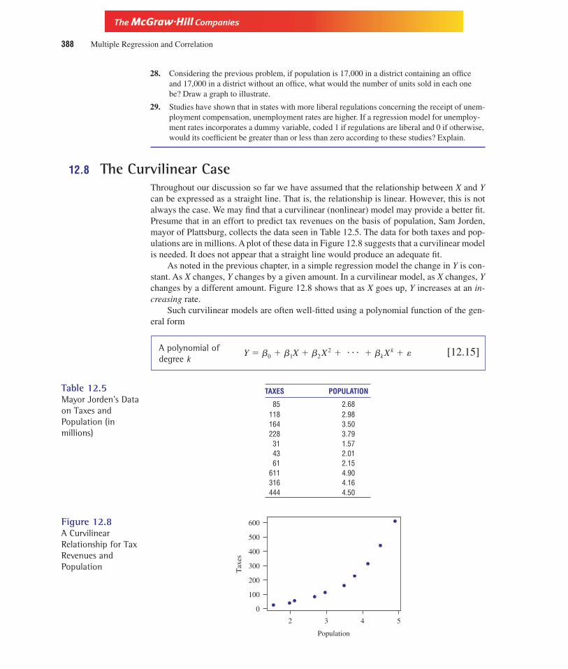
Version, Third Edition
28. Considering the previous problem, if population is 17,000 in a district containing an officeand 17,000 in a district without an office, what would the number of units sold in each onebe? Draw a graph to illustrate.
29. Studies have shown that in states with more liberal regulations concerning the receipt of unem-ployment compensation, unemployment rates are higher. If a regression model for unemploy-ment rates incorporates a dummy variable, coded 1 if regulations are liberal and 0 if otherwise,would its coefficient be greater than or less than zero according to these studies? Explain.
12.8 The Curvilinear CaseThroughout our discussion so far we have assumed that the relationship between X and Ycan be expressed as a straight line. That is, the relationship is linear. However, this is notalways the case. We may find that a curvilinear (nonlinear) model may provide a better fit.Presume that in an effort to predict tax revenues on the basis of population, Sam Jorden,mayor of Plattsburg, collects the data seen in Table 12.5. The data for both taxes and pop-ulations are in millions. A plot of these data in Figure 12.8 suggests that a curvilinear modelis needed. It does not appear that a straight line would produce an adequate fit.
As noted in the previous chapter, in a simple regression model the change in Y is con-stant. As X changes, Y changes by a given amount. In a curvilinear model, as X changes, Ychanges by a different amount. Figure 12.8 shows that as X goes up, Y increases at an in-creasing rate.
Such curvilinear models are often well-fitted using a polynomial function of the gen-eral form
A polynomial of degree k
[12.15]Y � b0 � b1X � b2X 2 � ≥ � bkXk � �
388 Multiple Regression and Correlation
Table 12.5Mayor Jorden’s Dataon Taxes andPopulation (inmillions)
TAXES POPULATION
85 2.68118 2.98164 3.50228 3.7931 1.5743 2.0161 2.15
611 4.90316 4.16444 4.50
Figure 12.8A CurvilinearRelationship for TaxRevenues andPopulation
600
500
400
2 3 4 5
300
200
100
0
Population
Tax
es

Version, Third Edition
Formula (12.15) is said to be a polynomial of degree k since that is the highest power of anyexplanatory variables. Mayor Jorden’s model might best be fitted using a polynomial of de-gree 2, or a second-order polynomial, such as
The quadratic formof the polynomial
[12.16]
which is the quadratic form of the model in which the second explanatory variable ismerely the square of the first. In the mayor’s case, it becomes
where T is taxes and POP is population.Let us compare the results of this model to those obtained if a simple linear model is es-
timated. The Minitab printout for the simple model in which taxes are regressed on popula-tion is shown in Display 12.7. Notice that the R2 value is a respectable 86.1 percent withof 84.3 percent and a standard error of 76.38. The entire model is
Display 12.7 A Linear ModelRegression Analysis
The regression equation isTAXES = -302 + 159 POP
Predictor Coef Stdev t-ratio pConstant -302.39 76.75 -3.94 0.004POP 158.96 22.60 7.04 0.000
s = 76.38 R-sq = 86.1% R-sq(adj) = 84.3%
If the quadratic model is used, as seen in the Minitab printout in Display 12.8, both the and the standard error improve to 98.7 percent and 22.20 respectively. The model becomes
Obviously, the quadratic model provides the better fit.
Display 12.8 A Quadratic FitRegression Analysis
The regression equation isTAXES = 325 - 278 POP + 67.7 POPSQ
Predictor Coef Stdev t-ratio pConstant 325.36 70.63 4.61 0.000POP -277.98 47.10 -5.90 0.000POPSQ 67.692 7.226 9.37 0.000
s = 22.20 R-sq = 99.0% R-sq(adj) = 98.7%
An alternative approach to curvilinear models can be achieved by transforming thedata in some manner. A common method of transformation involves the use of logarithms.This logarithmic transformation may make the data linear in the log. Table 12.6 showsMayor Jorden’s original data in the first two columns and their natural logarithms in the lasttwo columns. The mayor then simply regresses the log of taxes on the log of population, as
T � 325.36 � 277.98POP � 67.692(POP)2
R 2
T � �302.39 � 158.96POP
R 2
T � b0 � b1POP � b2(POP)2
Y � b0 � b1X � b2X 2
Chapter Twelve 389

Version, Third Edition
seen in the Minitab printout in Display 12.9. Note the further improvement in the standarderror and the of only 0.1680 and 97.2 percent, respectively. The model is
Display 12.9 A Logarithmic TransformationRegression Analysis
The regression equation isLOGTX = 2.03 + 2.61 LOGPOP
Predictor Coef Stdev t-ratio pConstant 2.0302 0.1724 11.78 0.000LOGPOP 2.6147 0.1478 17.69 0.000
s = 0.1680 R-sq = 97.5% R-sq(adj) = 82.2%
Then, if population is 3.2, log POP � 1.163 and
Taking the antilog of 5.071 yields 159.33; or, since the data were originally in millions, themayor’s tax receipts would be estimated at $159,330,000.
It may be necessary to experiment with different functional forms in order to deter-mine which provides the best fit. In search of the optimal model, the results from differentlogarithmic models may be compared with those obtained using polynomial functions. Theuse of computers makes this comparison practical.
The results of such comparisons may, however, prove inconsistent. One model mayreport a higher coefficient of determination than another (that’s good) while carrying ahigher standard error of the estimate (that’s bad). The question then becomes, whichmodel do you use?
The answer depends, at least in part, on the purpose for which the model is intended.If you wish to use the model to explain present values of Y and to understand why it be-haves as it does, use the model with the higher coefficient of determination. That is, if theintent is to explain, then the model with the higher explanatory value should be used.
If, on the other hand, the purpose of the model is to predict future values of Y, use themodel with the lower standard error of the estimate. If you want to predict, you will enjoygreater success with the model that generates the lower prediction error.
However, such experimentation should be kept to a minimum. It is considered ques-tionable, even unethical, to experiment wildly with first one model and then another. Youshould know from the outset, given the nature of your research study, what procedure should
� 5.071logTX � 2.0302 � 2.6147(1.163)
LOGTX � 2.0302 � 2.6147(LOGPOP)
R 2
390 Multiple Regression and Correlation
Table 12.6LogrithmicTransformation
Taxes POP LOGTX LOGPOP
85 2.68 4.44265 0.98582118 2.98 4.77068 1.09192164 3.50 5.09987 1.25276228 3.79 5.42935 1.3323731 1.57 3.43399 0.4510843 2.01 3.76120 0.6981361 2.15 4.11087 0.76547
611 4.90 6.41510 1.58924316 4.16 5.75574 1.42552444 4.50 6.09582 1.50408

Version, Third Edition
be followed. The analogy is often made that to search blindly for the best model is similar toshooting the arrow at the target and then drawing the bull’s-eye at the spot where the arrowlanded.
30. Plot the data below. Compare a linear model to the quadratic form and provide a comparativeevaluation of each. Using the better model, predict Y if X � 22.
Y X Y X
2170 31 731 182312 32 730 182877 36 815 197641 48 1408 252929 36 2768 35
1297 24
31. Using the data from Exercise 30, perform a logarithmic transformation and test the regressionresults. What are your observations?
32. Mayor Jorden wants to estimate tax revenues on the basis of new business formations. Hecollects the data displayed below from 22 cities he feels are similar to his.
a. Plot the scatter diagramb. Compare a linear model to a quadratic form. Which seems to give the best fit?c. Predict tax revenues if there are 68 new businesses.
City New Business Tax Revenues City New Business Tax Revenues
1 47 $10,154,589 12 68 $26,272,8982 51 18,215,568 13 47 6,074,6153 57 27,171,076 14 58 18,215,5684 68 26,272,898 15 51 13,546,4485 57 6,074,615 16 48 17,500,5446 45 5,693,092 17 65 14,801,0297 85 43,918,912 18 68 18,215,5688 87 46,334,860 19 85 43,918,9129 48 11,781,520 20 68 42,738,224
10 57 17,500,544 21 86 45,117,74811 68 26,272,898 22 58 25,391,750
33. Using the data from Exercise 32, compute the logarithmic regression model. How does itcompare to the one developed in the previous problem? Estimate taxes if there are 68 newbusinesses formed.
List of Formulas[12.1] The multiple regression model
[12.4] Standard error of the estimate
[12.5]Coefficient of multipledetermination
[12.8]Adjusted coefficient of multiple determination
[12.12] t-test for significance of bit �bi � bi
sbi
R 2 � 1 � (1 � R2)n � 1
n � k � 1
R2 �SSR
SST
Se � ��(Yi � Yi)2
n � k � 1
Y � b0 � b1X1 � b2X2 � ≥ � bkXk � �
Chapter Twelve 391
Section Exercises

Version, Third Edition
[12.13] Variance inflation factor for Xi
[12.14]The beta or standardized coef-ficient for Xi
[12.15] A polynomial of degree k
[12.16] The quadratic form of thepolynomial
Chapter ExercisesNote: Most of these problems require a computer.
34. A management director is attempting to develop a system designed to identify what personalattributes are essential for managerial advancement. Fifteen employees who have recentlybeen promoted are given a series of tests to determine their communication skills (X1), abilityto relate to others (X2), and decision-making ability (X3). Each employee’s job rating (Y ) is re-gressed on these three variables. The original raw data are as follows:
Y X1 X2 X3 Y X1 X2 X3
80 50 72 18 69 39 73 1975 51 74 19 68 40 71 2084 42 79 22 87 55 80 3062 42 71 17 92 48 83 3392 59 85 25 82 45 80 2075 45 73 17 74 45 75 1863 48 75 16 80 61 75 20
62 59 70 15
a. Develop the regression model. Evaluate it by determining whether it shows a significantrelationship among the dependent variable and the three independent variables.
b. What can be said about the significance of each Xi?
35. To what cause might you attribute the insignificance of X1 and X3 in Exercise 34? Obtain the cor-relation matrix for these variables and test each pair for multicollinearity. Set a � 5 percent.
36. Compare your results in Exercise 35 to those obtained based on VIF.
37. Should the management director in Exercise 36 use this model to identify characteristics thatmade an employee eligible for advancement?
38. As a class project, a team of marketing students devises a model that explains rent for studenthousing near their university. Rent is in dollars, SQFT is the square footage of the apartmentor house, and DIST is distance in miles from house to campus.
Rent SQFT DIST Rent SQFT DIST
220 900 3.2 400 1,290 1.5250 1,100 2.2 450 1,370 0.5310 1,250 1.0 500 1,400 0.5420 1,300 0.5 550 1,550 0.3350 1,275 1.5 450 1,200 0.5510 1,500 0.5 320 1,275 1.5
a. Devise the model. Is it significant at the 1 percent level?b. Evaluate the significance of both coefficients.c. Are the signs appropriate? Explain.
39. Evaluate the model from the previous problems. Does it appear useful in predicting rent? Explain.
Y � b0 � b1 X � b2 X 2
Y � b0 � b1 X � b2 X 2 � ≥ � bk X k � �
Beta �bi
sY�sXi
VIF(Xi) �1
1 � R2i
392 Multiple Regression and Correlation

Version, Third Edition
Chapter Twelve 393
40. Is there evidence of multicollinearity in the model from the previous problem? Does it invali-date the model for predicting rent? Why or why not?
41. From the model developed above for student rents, can you conclude distance from campus isa stronger determinant of rent than is square footage? Why or why not?
42. If two apartments have the same space, but one is 2 miles closer to campus, how will its rentdiffer from that of the more distant dwelling?
43. In order to expand their model on students’ rents, the marketing majors from the problems abovedevise a luxury index in which students rate the amenities of an apartment based on availablecomforts, such as swimming pools, tennis courts, maid service, and other luxuries to which stu-dents are traditionally accustomed. For the 12 observations above, this index measured 22, 23,35, 40, 32, 55, 36, 41, 51, 50, 48, and 29. Incorporate the variable in your model to explain rents.Analyze and explain why you got these results. Is your model better with this additional vari-able? What problem are you likely encountering, and what change would you make to correct it?
44. Make the change you suggested in the previous problem and discuss your results.
45. In the past, many economists have studied the spending patterns of consumers in the economy.A famous study by Milton Friedman concludes that consumption is a function of permanentincome, which is defined as the average level of income the consumer expects to receive wellinto the future. The habit-persistence theory of T. M. Brown argues that consumption is shapedby a consumer’s most recent peak income—the highest income received in the recent past.
To combine these two theories, an economist collected data on consumption (CONS),permanent income (PERM), and peak income (PEAK), and performed OLS to devise a model.Given these data, what did that model look like? (All values are in thousands of dollars.)
CONS PERM PEAK CONS PERM PEAK
12 15 17 14 17 2022 28 31 20 25 2915 19 21 17 21 2517 19 24 15 19 2219 24 27 16 20 26
a. Evaluate the model.b. Would multicollinearity explain the insignificance of PEAK? How can you tell?
46. The data shown here were collected to explain salary levels for workers at a local plant.
Salary ($1,000’s) Years of Education Sex
42.2 8 M58.9 12 M98.8 16 M23.5 6 F12.5 5 M67.8 12 M51.9 10 F81.6 14 F61.0 12 F
a. Compute the regression model, using a computer.b. Is there evidence of sex discrimination in salary levels?c. Is education useful in explaining salary?d. Are autocorrelation and heteroscedasticity problems?
47. You have just run a model regressing employee retention (in years) on age at hiring and gen-der, encoding the dummy variable for gender as 1 if male and 0 if female. The results were
Y � 3.2 � 0.65AGE � 1.3GENDER

Version, Third Edition
394 Multiple Regression and Correlation
a. What is the formula for male? For female?b. You then realize that you meant to encode 1 if female and 0 if male. What will the equa-
tion become?c. Now what is the formula for male? For female?d. Using the formula seen above, what is the estimate of years of retention if a male is hired
at age 23? What is it using your revised formula?
Computer ExerciseStudies in finance have shown that the price of a share of stock is directly related to the issuing com-pany’s level of debt and to the dividend rate, but is inversely related to the number of shares out-standing. Access the computer file STOCK from your data disk. PRICE and the dividend rate, DI-VRATE, are in dollars, DEBT is in millions of dollars and the number of shares outstanding,OUTSTD, is in millions of shares. Using PRICE as the dependent variable, evaluate the model. Pro-vide all relevant statistical interpretations and conclusions. Prepare your final statistical report as de-scribed in Appendix I.
C U R T A I N C A L LYour assignment as an intern for GriffenAssociates, described in Setting theStage at the opening of the chapter,
briefly illustrated the need to analyze the performance ofseveral competitive mutual funds. You are to developmodels that will examine three-year returns and comparethem to the one-year returns of these funds, using as ex-planatory variables the turnover rates (the percentage ofthe funds bought and sold over each time period in ques-tion), initial total assets in billions of dollars at the time thefund was opened, and whether the fund carries a sales
load. This last variable is encoded as 1 if it has a load, andno-load funds are encoded as 0.
Your supervisor at Griffen wants you to prepare afull report, including all statistical analysis presented inthis chapter. You must specify the models for both one-year and three-year returns for both load and no-loadfunds. Tests for multicollinearity must be conducted alongwith all relevant statistical analysis. Using the data pro-vided here, prepare your statistical report as described inAppendix I.
Three-year One-year Three-year One-yearReturn Return Load Turnover Turnover Assets
5.6 0.1 0 112 58 220.004.7 1.9 1 95 62 158.004.5 2.6 1 241 65 227.254.8 2.0 1 87 61 242.405.7 3.5 0 98 57 287.854.1 �4.3 1 102 66 207.054.7 3.2 1 72 63 237.354.1 �4.1 1 96 65 207.055.2 2.2 0 78 59 262.603.7 2.1 1 118 87 186.856.2 5.3 0 98 47 313.106.6 11.0 0 87 41 333.305.2 0.3 0 117 61 262.605.5 �2.1 0 87 46 277.755.6 4.7 0 85 35 282.80

Version, Third Edition
Chapter Twelve 395
From the Stage to Real LifeIn the Chapter 3 From the Stage to Real Life exercise, we became familiar with some mu-tual funds investor information sites and with the Vanguard Group of Funds in particular.Here we will look at more detailed information that is routinely reported about the fundsand their performance. This chapter’s Curtain Call analysis required information aboutloads (fees), assets, and 1- and 3-year returns. Is this information available at mutual fundscompany web sites? Let’s look at three major mutual funds companies.
At the Vanguard Group (www.vanguard.com) Home Page, select the “mutual funds”icon. Next, clock on “Funds by Category.” In the Growth funds, select the “U.S. GrowthPortfolio.” Click through the tabs on the folders and make notes on where to obtain data onloads, assets, and 1- and 3-year returns.
Do the same for Fidelity Funds (www.fidelity.com). At the Home Page, go to “Fund In-formation.” In the search area, type in “Emerging Growth” and click the “go.” Note theavailable data.
Repeat this again for the Dreyfus Funds (www.dreyfus.com). At the Home Page, select“Mutual Funds” under the Products heading, and then click on “Growth” funds. Look atthe Emerging Leaders Fund information for the availability of this same data.

Version, Third Edition
396
C H A P T E R13Time Seriesand Index Numbers

Version, Third Edition
397
Laspeyresindex
Paascheindex
Time-Series Analysis
Four componentsof a time-series
Trendanalysis
Decomposition ofa time-series
Time-series data
Simple indexnumber
A compositeprice index
Weightedcomposite
indexes
Index numbers
Moving averages
Exponentialsmoothing
Smoothing techniques
Chapter BlueprintThis chapter examines the use of time-series data and their application to common business situa-tions. The manner in which index numbers are used to make time series data more comparable overtime is also demonstrated.

Version, Third Edition
13.1 IntroductionThe importance of being able to forecast the future with some degree of accuracy cannotbe overstated. Imagine the results if you could gaze into a crystal ball and predict the fu-ture on the first Saturday in May when the Kentucky Derby is held, or just before kickofffor the next Super Bowl. Your success rate in predicting winners would no doubt sky-rocket!
Such is the case in the business world. The ability to forecast and predict future eventsand trends greatly enhances the likelihood of success. It is therefore no wonder that busi-nesses spend a good deal of time and effort in the pursuit of accurate forecasts of futurebusiness trends and developments.
Numerous quantitative tools can be used to develop useful forecasts. By relying onthese tools, you can build your own crystal ball and use it to peer into the future. This
398 Time Series and Index Numbers
S E T T I N G T H E S T A G EOver the past few yearsDickson Industries has en-joyed considerable growth
in sales revenues and profits. Much of thissuccess is due to hard work by JeremyDickson, owner and chief executive officerof the business, as well as that of his closeand trusted staff. Mr. Dickson has alwaysrelied heavily on careful planning based ona thorough analysis of market conditions.
This analysis is often designed to detectfuture movements in business activity and todetermine whether the present trend will con-tinue. Mr. Dickson also insists that his staffexamine any cyclical activity in businessfluctuations over the course of several years.
Furthermore, Mr. Dickson observesany detectable patterns regularly occurringat specific times within the year or duringcertain seasons in planning his operations.He has noticed that his business is quite sea-sonal, in that his profits are usually higher atcertain times of the year.
However, Mr. Dickson realizes that theupward trend in sales he has experienced isnot as favorable as it may seem. Changes inthe economic climate over time affect thevalues of his profits and sales revenues. Hetherefore recognizes the need to index thesemeasures of business performance to get amore accurate impression of just how wellhis business is doing.
30
0 5 10 15
20
10
Time
Linear Trend ModelYt = 8.375 + 1.43382*t
Sales Revenues for Dickson Industries
Sale
s
ActualFitsActualFits
MAPE: 7.31643MAD: 1.49449MSD: 4.18428

Version, Third Edition
chapter examines ways in which time-series data can be used to make forecasts, and howthose forecasts can be used to make informed decisions.
13.2 Time Series and Their ComponentsThe process of developing a forecast starts with the collection of past data for several timeperiods. The resulting data set is called a time series because it contains observations forsome variable over time. The time periods can vary in length. They can be yearly, quar-terly, monthly, or even daily. Time periods of only one hour may be used for highlyvolatile variables such as the price of a heavily traded stock on one of the organizedexchanges.
Time Series A collection of data for some variable or set of variables over severaltime periods.
Table 13.1 contains quarterly sales data for Rampart Industries in millions of dollars where,for example, 1998-III is the third quarter of the year 1998.
Chapter Thirteen 399
Sales SalesTime period (in millions) Time period (in millions)
1995-IV 31.1 1997-II 61.81996-I 35.6 III 75.9
II 42.8 IV 74.1III 50.3 1998-I 88.7IV 49.2 II 79.1
1997-I 62.0 III 92.5
Table 13.1Quarterly SalesFigures for RampartIndustries
The purpose of time-series analysis is to predict or forecast future values of the vari-able from past observations. One direct approach is the naive method of forecasting,which presumes that the best predictor of the value of the variable in the next time periodis its value in the current time period. In its simplest form it can be expressed as
The naive forecasting model [13.1]
where is the estimate of the value of the time series in the next time period t � 1 andYt is the actual value in the current time period t. This approach is often used when the dataexhibit a random walk. Random walk movements exhibit no trend upward or downwardand typically shift direction suddenly. Such movements are analogous to an individual outfor a evening stroll to nowhere in particular. When he comes to an intersection he randomlydecides, perhaps by flipping a coin, which way to turn. Such randomness cannot be pre-dicted, and the best we can do is use the most recent observation as our prediction for thenext value. This method of forecasting is most successful for data that are collected forshort time intervals such as on a daily or a weekly basis.
However, most time series are more complex than that. All times series contain at leastone of the following four components: (1) secular trend; (2) seasonal variation; (3) cyclical
Yt�1
Yt�1 � Yt

Version, Third Edition
variation; or (4) irregular, or random, variation. The remainder of this section examineseach of these time-series components.
A. Secular TrendThe secular trend, or merely the trend, is the long-run behavior of the variable over an ex-tended length of time. It reflects the general direction of the time series as upward or down-ward. Examples include the rising number of foreign cars sold in the United States, the in-crease in the volume of credit transactions over the past few years, and the downwardmovement in the number of people living in rural areas in the last two decades.
Secular Trend The continuous long-term movement in a variable over an extendedperiod of time.
Figure 13.1 shows the trend in output for Rampart Industries for the past decade. Al-though the data show considerable variation above and below the trend line drawn throughthe middle of the data, the secular trend is unmistakably upward.
400 Time Series and Index Numbers
130
1989 1990 1991 1992 1993 1994 1995 199819971996
120
110
Year
Out
put Trend
line
Actualdata
Figure 13.1Trend Line forRampart Industries(annual output)
B. The Seasonal ComponentA lot of business activity is influenced by changing seasons of the year. For example, salesof certain seasonal goods such as Honda snowmobiles, Jantzen swimwear, and HallmarkValentine cards would likely display a strong seasonal component. Seasonal fluctuationsare patterns that tend to reoccur regularly during the time period. Although we often thinkof seasonal variations as occurring regularly each year, such as the annual sales of Christ-mas hams, the time period in question can be much shorter. The daily influx of customersat the lunch counter each noon is an example. If the seasonal variation does occur on ayearly basis, annual data will not capture or reflect these changes. The data must be col-lected on a quarterly, monthly, or even weekly basis.
Seasonal Fluctuations Movements in the time series that reoccur each year aboutthe same time.
Figure 13.2 shows that each year the unemployment rate tends to go up in May whenhigh school students enter the summer job market, and that it goes down in Novemberwhen retail stores hire temporary help to handle the Christmas rush. Notice that no appar-ent trend exists in the unemployment rate.

Version, Third Edition
C. Cyclical VariationsMany variables exhibit a tendency to fluctuate above and below the long-term trend over along period of time. These fluctuations are called cyclical fluctuations or business cycles.They cover much longer time periods than do seasonal variations, often encompassingthree or more years in duration.
Cyclical Fluctuations Wavelike variations in the general level of business activityover a relatively long time period.
A cycle contains four phases: (1) the upswing or expansion, during which the level ofbusiness activity is accelerated, unemployment is low, and production is brisk; (2) the peak,at which point the rate of economic activity has “topped out”; (3) the downturn, or con-traction, when unemployment rises and activity wanes; and (4) the trough, where activityis at the lowest point. A cycle runs from one phase to the next like phase and, as shown inFigure 13.3, fluctuates above and below the long-term trend in a wavelike manner.
Chapter Thirteen 401
1985 19951980 199019701965 1975
Num
ber
of a
utos Trend line
Figure 13.3Cyclical Fluctuationsof Foreign AutoImports
DecJulyJuly JanJan DecJulyJan Dec
Perc
ent o
f la
bor
forc
e un
empl
oyed
Figure 13.2SeasonalFluctuations inUnemployment
D. Irregular FluctuationsTime series also contain irregular, or random, fluctuations caused by unusual occur-rences producing movements that have no discernible pattern. These movements are, likefingerprints and snowflakes, unique, and unlikely to reoccur in similar fashion. They canbe caused by events such as wars, floods, earthquakes, political elections, or oil embargoes.

Version, Third Edition
13.3 Time-Series ModelsA time-series model can be expressed as some combination of these four components. Themodel is simply a mathematical statement of the relationship among the four components.Two types of models are commonly associated with time series: (1) the additive model and(2) the multiplicative model. The additive model is expressed as
where Yt is the value of the time series for time period t, and the right-hand side values arethe trend, the seasonal variation, the cyclical variation, and the random or irregular varia-tion, respectively, for the same time period. In the additive model, all values are expressedin original units, and S, C, and I are deviations around T. If we were to develop a time-series model for sales in dollars for a local retail store, we might find that T � $500,S � $100, C � �$25, and I � �$10. Sales would be
Notice that the positive value for S indicates that existing seasonal influences have had apositive impact on sales. The negative cyclical value suggests that the business cycle iscurrently in a downswing. There was apparently some random event that had a negativeimpact on sales.
The additive model suffers from the somewhat unrealistic assumption that the compo-nents are independent of each other. This is seldom the case in the real world. In most in-stances, movements in one component will have an impact on other components, therebynegating the assumption of independence. Or, perhaps even more commonly, we often findthat certain forces at work in the economy simultaneously affect two or more components.Again, the assumption of independence is violated.
As a result, the multiplicative model is often preferred. It assumes that the componentsinteract with each other and do not move independently. The multiplicative model is ex-pressed as
In the multiplicative model, only T is expressed in the original units, and S, C, and I arestated in terms of percentages. For example, values for bad debts at a commercial bankmight be recorded as T � $10 million, S � 1.7, C � 0.91 and I � 0.87. Bad debts couldthen be computed as
Since seasonal fluctuations occur within time periods of less than one year, they wouldnot be reflected in annual data. A time series for annual data would be expressed as
13.4 Smoothing TechniquesThe general behavior of the variable can often be best discussed by examining its long-term trend. However, if the time series contains too many random fluctuations or short-term seasonal changes, the trend may be somewhat obscured and difficult to observe. It ispossible to eliminate many of these confounding factors by averaging the data over severaltime periods. This is accomplished by using certain smoothing techniques that removerandom fluctuations in the series, thereby providing a less obstructed view of the true
Yt � Tt � Ct � It
Y � (10)(1.7)(0.91)(0.87) � $13.46 million
Yt � Tt � St � Ct � It
� $565
Y � $500 � $100 � $25 � $10
Yt � Tt � St � Ct � It
402 Time Series and Index Numbers

Version, Third Edition
behavior of the series. We examine two common methods of smoothing time-series data: amoving average and exponential smoothing.
A. Moving AveragesA moving average (MA) will have the effect of “smoothing out” the data, producing amovement with fewer peaks and valleys. It is computed by averaging the values in the timeseries over a set number of time periods. The same number of time periods is retained foreach average by dropping the oldest observation and picking up the newest. Assume thatthe closing prices for a stock on the New York Stock Exchange for Monday throughWednesday were $20, $22, and $18, respectively. We can compute a three-period (day)moving average as
(20 � 22 � 18)�3 � 20
This value of 20 then serves as our forecast or estimate of what the closing price might beat any time in the future. If the closing on Thursday is, say, 19, the next moving average iscalculated by dropping Monday’s value of 20 and using Thursday’s closing price of 19.Thus, the forecast becomes
The estimate figured in this manner is seen as the long-run average of the series. It istaken as the forecast for the closing price on any given day in the future.
Moving Average (MA) A series of arithmetic averages over a given number of timeperiods; the estimate of the long-run average of the variable.
Consider the sales for Arthur Momitor’s Snowmobiles, Inc., over the past 12 monthsas shown in Table 13.2. Both a three-month MA and a five-month MA are calculated. Weobtain the first entry in the three-month MA by averaging the sales of snowmobiles inJanuary, February, and March. The resulting value of (52 � 81 � 47)�3 � 60 is centeredon the middle time period of February. We determine the next entry by averaging February,March, and April, and centering the value of 64.33 in the middle of those three periods,which is March. The remaining entries are determined similarly.
The first entry in the five-month MA series uses values for months January throughMay. The average of (52 � 81 � 47 � 65 � 50)�5 � 59 is centered in the middle ofthose five time periods at March.
(22 � 18 � 19)�3 � 19.67
Chapter Thirteen 403
Table 13.2Snowmobile Salesfor Arthur Momitor
Month Sales ($100) Three-Month MA Five-Month MA
January 52February 81 60.00March 47 64.33 59.00April 65 54.00 63.20May 50 62.67 56.00June 73 56.00 58.60July 45 59.33 55.60August 60 51.67 61.40September 50 63.00 55.80October 79 58.00 59.20November 45 62.00December 62

Version, Third Edition
Moving averages have the effect of smoothing out large variations in the data. Thissmoothing effect occurs because unusually large or unusually small observations are aver-aged in with other values, and their impact is thereby restrained. The larger the number oftime periods in a moving average, the more pronounced the smoothing effect will be. No-tice that the range of values in the three-month MA is less than that in the original data andgreater than the range found in the five-month MA. Figure 13.4 illustrates this tendency forthe smoothing effect to increase with the number of time periods in the moving average.
Notice that when an odd number of time periods is used in the moving average, the re-sults can be automatically centered at the middle time period. When Arthur Momitor cal-culated his three-period moving average for snowmobiles, the first value, for example,could be readily centered at the middle time period of February.
404 Time Series and Index Numbers
Figure 13.4Comparing MovingAverages
Seriesvalues
Time
Original data
3–term moving average
5–term moving average
However, if there is an even number of time periods in the moving average, an ad-justment must be made because there is no middle observation at which the value isautomatically centered. Consider the quarterly sales data for Sun Shine Greetings Cards inTable 13.3. The data run from the first quarter of 1996 to the last quarter of 1998. If a four-period (quarter) moving average is to be calculated, the first entry of 42.50 is obtained byaveraging the data for all four quarters of 1996. This value, however, does not correspondto any specific time period in the original data series, but is set between the second and thirdquarters of 1996. The remaining entries are similarly off center.
It is necessary to center the moving average by taking the mean of each successivepair of moving averages. Thus, the average of the first and second values yields
(42.50 � 45.75)�2 � 44.13
Table 13.3Sales for Sun ShineCards ($1,000)
CenteredTime Period Sales Four-Quarter MA Four-Quarter MA
1996-I 40II 45III 38
42.5044.13
IV 4745.75
45.001997-I 53
44.2545.38
II 3946.50
44.63III 47
42.7542.50
IV 3242.25
43.001998-I 51
43.7542.50
II 4541.25
44.00III 37
46.75
IV 54

Version, Third Edition
which is then centered at the third quarter. The next entry of 45.00 is obtained by averag-ing the second and third values, yielding
which is centered at the fourth quarter of 1996. The remaining values are likewise centeredat their respective time periods.
Moving averages can be used to remove irregular and seasonal fluctuations. Eachentry in the moving average is derived from four observations of quarterly data—that is,one full year’s worth. Thus, the moving average “averages out” any seasonal variations thatmight occur within the year, effectively eliminating them and leaving only trend and cycli-cal variations.
In general, if the number of time periods in a moving average is sufficient to encompassa full year (12 if monthly data are used; 52 if weekly data are used), seasonal variations areaveraged out and removed from the series. The data are then said to be deseasonalized.
As noted, the use of a larger number of time periods results in a smoother averaged se-ries. Therefore, if the data are quite volatile, a small number of periods should be used inthe forecast to avoid placing the forecast too close to the long-run average. If the data donot vary greatly from the long-run mean, a larger number of time periods should be used informing the moving average.
Minitab Display 13.1 shows the Minitab printout for the Sun Shine cards illustration.Example 13.1 further demonstrates the moving average principle.
Minitab Display 13.1Four-Period Moving Average for Sun Shine Cards
Row Period C1 . MA Predict Error
1 1 40 * * *2 2 45 * * *3 3 38 44.125 * *4 4 47 45.000 * *5 5 53 45.375 * *6 6 39 44.625 44.125 -5.1257 7 47 42.500 45.000 2.0008 8 32 43.000 45.375 -13.3759 9 51 42.500 44.625 6.375
10 10 45 44.000 42.500 2.50011 11 37 * 43.000 -6.00012 12 54 * 42.500 11.500
(45.75 � 44.25)�2 � 45.00
Chapter Thirteen 405
60
50
40
0 42 1086 12 14
30
Time
Sale
s
ActualPredictedForecastActualPredictedForecast
MAPE: 16.3945MAD: 6.6964MSD: 60.6138
Moving AverageLength 4
0

Version, Third Edition
Example 13.1 TransAmerica Trucking has collected data for the last 10 months on the tonnage of ship-ments. Assist their research department by computing the three-term moving average.What is your forecast for shipments in the future?
Solution:Month Shipments Three-Period MA Month Shipments Three-Period MA
1 70 6 81 76.672 68 71.00 7 82 77.333 75 74.00 8 69 74.334 79 73.67 9 72 69.675 67 75.67 10 68
The first three values of 70, 68, and 75 average to 71. The values for periods two throughfour of 68, 75, and 79 average to 74. The process continues until the last observation is en-countered. The forecast for any future month is 69.67 tons.
Interpretation: Since the data do not exhibit any trend up or down, the moving average technique is suitedto forecast future shipments. The forecast of 69.67 will of course change when the ship-ment for the eleventh month is reported and the moving average for month 10 is computed.
B. Exponential SmoothingAs the name implies, exponential smoothing has the effect of smoothing out a series. It alsoprovides an effective means of prediction. First-order exponential smoothing is usedwhen the data do not exhibit any trend pattern. The model contains a self-correcting mech-anism that adjusts forecasts in the opposite direction of past errors. The equation is
Exponential smoothing [13.2]
where Ft�1 is the forecast for the next time periodAt is the actual, observed value for the current time periodFt is the forecast previously made for the current time period
The a is a “smoothing constant” which is given a value between 0 and 1. Since the data donot trend up or down but fluctuate around some long-run average, we take the value Ft�1 asthe forecast for any future time period.
Exponential Smoothing A forecasting tool in which the forecast is based on aweighted average of current and past values.
As an illustration, suppose it is currently the last business day of February. Sales forUncle Vito’s Used Cars for the month total $110 thousand. Uncle Vito has decided to fore-cast sales for March. According to Formula [13.2], the March forecast, Ft�1, requires
1. February’s actual sales, At.
2. The forecast for February, Ft.
Ft�1 � aAt � (1 � a)Ft
406 Time Series and Index Numbers

Version, Third Edition
However, since March is the first month in which Uncle Vito is developing his forecast,there was no forecast made for February and Ft is unknown. The general practice is to sim-ply use the actual value of the previous time period, January in this case, for the first fore-cast. Uncle Vito’s records show that January sales were $105 thousand. Assuming a valueof 0.3 for a, the forecast for March is
As Table 13.4 reveals, Uncle Vito can plan for sales of $106.5 thousand. If actual salesin March are $107 thousand, the error is computed as Ft � At � 106.5 � 107 � �0.5. Also,FApr � (0.3)(107) � (0.7)(106.5) � 106.65.
� $106.5 thousand as the forecast for sales in March
� (0.3)(110) � (0.7)(105)� aAFeb � (1 � a)FFeb
Ft�1 � aAt � (1 � a)Ft
Chapter Thirteen 407
Table 13.4Uncle Vito’s AutoSales ($1,000)
Month Forecast Actual Error (Ft � At)
January – 105February 105 110 �5.0March 106.5 107 �0.5April 106.65 112 �5.35
Assume sales in April prove to be $112 thousand. The error is then �$5.35 thousand.Uncle Vito can also predict sales for May:
Of course, the value selected for a is crucial. Since we desire to produce a forecastwith the smallest possible error, the a-value that minimizes the mean square error (MSE)is optimal. Trial and error often serves as the best method to determine the proper a-value.Table 13.5 contains Uncle Vito’s actual sales data for the first seven months. Errors arebased on forecasts calculated using a-values of 0.3 and 0.8. The MSE is
Mean square error [13.3]MSE ��(Ft � At)
2
n � 1
� $108.26 thousand
� (0.3)(112) � (0.7)(106.65)FMay � aAApr� (1 � a)FApr
Ft�1 � aAt � (1 � a)Ft
Table 13.5Sales Data for UncleVito
Forecast ForecastMonth Actual (a � 0.3) Error (a � 0.8) Error
January 105February 110 105.00 �5.00 105.00 �5.00March 107 106.50 �0.50 109.00 2.00April 112 106.65 �5.35 107.40 �4.60May 117 108.26 �8.74 111.08 �5.92June 109 110.88 1.88 115.82 6.82July 108 110.32 2.32 110.36 2.36August 109.62 108.47

Version, Third Edition
408 Time Series and Index Numbers
For � 0.3, the MSE is
An a of 0.8 yields
An a of 0.8 produces better forecasting results since it generates a smaller error factor.Other values of a may be tried to determine their impact on MSE and the accuracy of theresulting forecasts. Generally speaking, if the data are rather volatile, a lower a-value iscalled for. This is because smaller values for a assign less weight to more recent observa-tions. If the data show considerable movement, the last observation may not be representa-tive of the long-run average.
Remember, first-order exponential smoothing in the manner described here is appro-priate if the data show no trend, but move around some average value over the long run. Ifa downward or an upward trend can be detected by plotting the data, second-order expo-nential smoothing, the mechanics of which will not be examined here, should be used.
Example 13.2 Predicting Unemployment RatesMonthly unemployment rates for 1997 are shown here. As an analyst for the U.S. Depart-ment of Labor, you are to (1) smooth out the fluctuations using a moving average with fourtime periods, and (2) use an exponential smoothing model with a set at 0.4 to forecast un-employment for some future month. The data do not show any pronounced trend up ordown.
January 5.4 July 5.4February 5.1 August 5.5March 5.0 September 5.2April 5.2 October 5.5May 5.3 November 5.1June 5.3 December 5.4
Solution:Month Rate MA Centered MA Ft
1997 January 5.4February 5.1 5.4March 5.0
5.1755.163 5.28
April 5.25.150
5.175 5.17May 5.3
5.2005.250 5.18
June 5.35.300
5.338 5.23July 5.4
5.3755.363 5.26
August 5.55.350
5.375 5.31September 5.2
5.4005.363 5.39
October 5.55.325
5.313 5.31November 5.1
5.3005.39
December 5.4 5.271998 January 5.32
� 22.88
MSE �(�5)2 � (2)2 � (�4.6)2 � (�5.92)2 � (6.82)2 � (2.36)2
7 � 1
� 23.20
MSE �(�5)2 � (�0.5)2 � (�5.35)2 � (�8.74)2 � (1.88)2 � (2.32)2
7 � 1

Version, Third Edition
Chapter Thirteen 409
The table shows the first moving average of 5.175, calculated by averaging rates forJanuary through April. It is situated in the middle of those four months between Februaryand March. The second entry of 5.150 is the average of the months February throughMay and is placed between March and April. The remaining values for MA are figuredsimilarly. These values are then centered by averaging successive pairs of moving av-erages.
To forecast using exponential smoothing, you must compute all forecasted figures forFebruary through December in order to obtain FDec � 5.27, which you then use in theJanuary 1998 forecast:
Interpretation: The moving average method forecasts a rate of 5.313 percent. Exponential smoothing pro-vides a forecast of 5.32 percent. This value (of 5.313 percent or 5.32 percent) is the fore-cast for January, or for any future time period, since the data do not exhibit a trend but arethought to fluctuate around this long-term average.
Unlike moving averages, which use only a set number of time periods of data, expo-nential smoothing uses all past values of the time series. This is because Ft�1 depends on At
and Ft. Yet, Ft used At�1 and Ft�1 in its calculation, and Ft�1 used At�2 and Ft�2. Thus, eachforecast depends on previous actual values of At�n all the way back to where the forecastsfirst began. The further back in time you go, the less impact a value of A has on the currentforecast.
1. If the data in a time series have a large variance, should a moving average with a large numberof time periods or one with a small number of time periods be used? Why?
2. Why should a moving average be used only when the data exhibit no upward or downwardtrend?
3. The number of daily telephone calls coming into a switchboard at a busy office are shownbelow. Calculate the 3-period moving average.
Day 1 2 3 4 5 6 7 8 9 10 11Calls 40 37 45 32 42 47 39 47 41 36 38
4. The daily numbers of employees absent from their jobs at a large factory are shown here. Cal-culate the four-period moving average associated with these data. Center the averages.
Day 1 2 3 4 5 6 7 8 9 10 11 12Employees 45 54 63 39 42 31 48 54 64 36 41 52
5. Excess inventories for Mom’s Apple Pies, Inc., over the past 10 weeks have been 101, 122,109, 111, 120, 117, 115, 118, 112, and 117. Using exponential smoothing, set alpha at 0.20 andforecast inventories for the eleventh week.
6. Monthly loans at the local bank in thousands of dollars are 211, 234, 209, 217, 215, 232, 221,211 and 203. Use exponential smoothing to forecast loans for the next time period using analpha value of 0.10. Calculate the mean square error and compare it to the mean square error ifalpha is 0.80. Which alpha value provides the best forecast?
� 5.32%
� (0.4)(5.4) � (0.6)(5.27)FJan � a(ADec) � (1 � a)(FDec)
Section Exercises

Version, Third Edition
13.5 Trend AnalysisIf a time series has a long-term trend upward or downward (like Figure 13.1 for example),trend analysis can be useful in developing forecasts. That is, if a trend is present in that thedata do not fluctuate around some long-run average like those for Sun Shine Cards dis-cussed above, smoothing methods such as moving averages and exponential smoothing arenot appropriate. Instead, a trend line can be estimated using the techniques of simpleregression discussed in Chapter 11. The dependent variable is the time series we wish toforecast, and time is used as the independent variable. The model to be estimated is thensimply
Trend line using simple regression [13.4]
Consider the data for the number of housing starts (in hundreds) in Happy Valley, Califor-nia, seen in Table 13.6. Mayfield Construction wants to fit this time series using OLS to de-velop a model to predict future housing starts.
Yt � b0 � b1t
410 Time Series and Index Numbers
Table 13.6Housing Starts inHappy Valley(in 100’s)
HousingYear t (X) Starts (Y ) XY X 2
1983 1 7.0 7.0 11984 2 7.1 14.2 41985 3 7.9 23.7 91986 4 7.3 29.2 161987 5 8.2 41.0 251988 6 8.3 49.8 361989 7 8.1 56.7 491990 8 8.6 68.8 641991 9 8.8 79.2 811992 10 8.9 89.0 1001993 11 8.7 95.7 1211994 12 9.1 109.2 1441995 13 9.4 122.2 1691996 14 9.1 127.4 1961997 15 9.5 142.5 2251998 16 9.9 158.4 256
136 135.9 1,214.0 1,496.0
The values for t are obtained by coding each time period starting with 1 for the firsttime period, 2 for the second, and so on. As we learned in Chapter 11, the sums of squaresand cross-products, used to calculate the regression line, are
Sum of the squares of X [13.5]
� 340
� 1,496 �(136)2
16
SSx � �X 2 �(�X)2
n

Version, Third Edition
Sum of the squaresof cross-products
[13.6]
The formulas for b1 and b0 are
Slope of the trend line [13.7]
Intercept of trend line [13.8]
The equation for the trend line is
Figure 13.5 displays the raw data and the trend line they produce.
Yt � 7.02 � 0.173t
� 7.02
b0 � Y � b1X
� 0.173
�58.85
340
b1 �SSxy
SSx
� 58.85
� 1,214 �(136)(135.9)
16
SSxy � �XY �(�X)(�Y)
n
Chapter Thirteen 411
Figure 13.5
’98’84 ’85 ’86 ’87 ’88 ’89 ’91 ’92 ’93 ’94 ’95 ’96 ’9719901983
Hou
sing
sta
rts
(000
)
10.0
6.0
6.5
7.07.027.5
8.0
8.5
9.0
9.5
Given this equation, it is possible to predict the number of housing starts for futuretime periods merely by substituting the appropriate value for t. Suppose Mayfield Con-struction wants to forecast the housing starts for 1999. Since the value of t would be 17 in

Version, Third Edition
1999, the forecast becomes
or 9,960 starts, since the data were expressed in units of 1,000.Similarly, since 2001 would carry a t value of 19, the forecast for 2001 would be
It is estimated that there will be 1,031 housing starts in 2001.Of course, the further into the future a forecast is made, the less confidence you can
place in its precision. Additionally, its accuracy is based on the condition that the past pro-vides a representative picture of future trends.
Example 13.3 Larry’s Lawn Service advertises a new chemical to kill weeds. To determine the trend inthe number of customers, Larry consults company records and finds the data shown here.He wishes to forecast customers for future time periods.
Time Period t (X ) Customers (Y ) XY X 2
1997 January 1 41 41 1February 2 43 86 4March 3 39 117 9April 4 37 148 16May 5 42 210 25June 6 35 210 36July 7 30 210 49August 8 31 248 64September 9 32 288 81October 10 30 300 100November 11 28 308 121December 12 28 336 144
1998 January 13 29 377 169February 14 26 364 196
105 471 3,243 1,015
Solution:
The equation for the trend line is
Yt � 43.2 � 1.27t
� 43.2
� 33.64 � ( � 1.27)(7.5)b0 � Y � b1X
b1 � � 1.27
� � 289.5
SSxy � 3,243 �(105)(471)
14
� 227.5
SSx � 1,015 �(105)2
14
� 10.31
Y � 7.02 � 0.173(19)
� 9.96
Y � 7.02 � 0.173(17)
412 Time Series and Index Numbers

Version, Third Edition
If Larry wished to forecast the number of customers his firm might get in March 1998,which would be time period 15, he would have
The forecast for August is
Interpretation: The negative coefficient for t of �1.27 tells Larry that business is trending downward at therate of 1.27 customers each time period (month).
7. Below are annual national test scores for high school seniors applying to colleges. Develop atrend line and forecast the test score for 1998.
1989 1990 1991 1992 1993 1994 1995 1996 1997
Score 412 423 453 432 541 539 587 591 602
8. The research department for National Industries has recorded the level of output in thousandsof units produced over the past several months. Using the data shown here, develop a trendline and forecast output for November and December.
January February March April May June July August
Output 89 78 71 75 68 61 65 54
9. City Utilities has undergone rapid expansion over the past several years. This growth has re-quired additions to its labor force each year. Use trend analysis to predict the size of the laborforce (in hundreds) in the year 2000.
1990 1991 1992 1993 1994 1995 1996 1997 1998
Employees 3.5 4.8 5.2 4.9 5.6 5.2 6.5 7.8 8.5
13.6 Time-Series DecompositionIt often proves useful to decompose a time series by “breaking-out” each of its four com-ponents. Thus, we can examine each component individually. The historic trend can reflectpast patterns of behavior, allowing us to gain insight into the long-run movements of thevariables we wish to examine. This permits the development of trend models useful in pre-diction and forecasting, as we saw in the previous section dealing with trend analysis. Byexamining the seasonal factor we can determine whether business activity exhibits any sea-sonal variation that must be considered in formulating future plans. For example, if wemarket swimwear or some other seasonal product we may find that sales are much higherin the spring than in the fall or winter. In addition, the cyclical performance of our businessmay also influence the direction of business planning.
A. Isolating the Seasonal ComponentThe first step in decomposition is to obtain a seasonal index. Consider the data inTable 13.7 for Vinnie’s Video Village. A superficial examination reveals that profits seemto be higher during the summer months when school is out, and lower at other times of theyear. This suggests the presence of seasonal factors.
� 16.53 customers
YAug � 43.2 � 1.27(21)
� 24.15, or 24 customers
YMar � 43.2 � 1.27(15)
Chapter Thirteen 413
Section Exercises
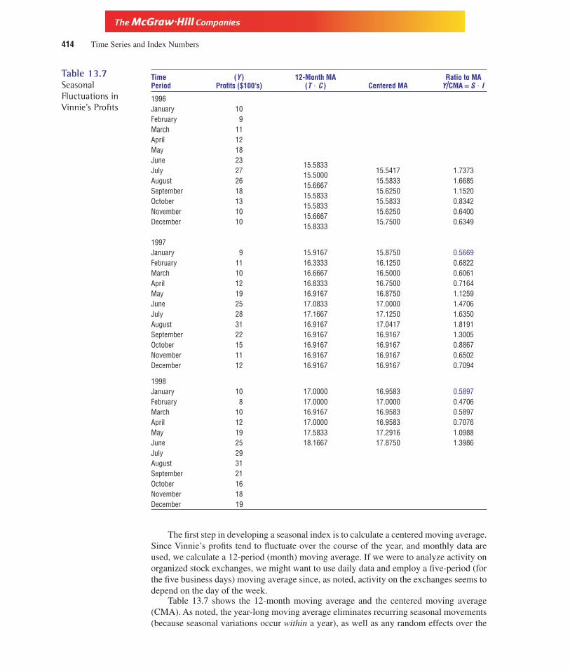
Version, Third Edition
The first step in developing a seasonal index is to calculate a centered moving average.Since Vinnie’s profits tend to fluctuate over the course of the year, and monthly data areused, we calculate a 12-period (month) moving average. If we were to analyze activity onorganized stock exchanges, we might want to use daily data and employ a five-period (forthe five business days) moving average since, as noted, activity on the exchanges seems todepend on the day of the week.
Table 13.7 shows the 12-month moving average and the centered moving average(CMA). As noted, the year-long moving average eliminates recurring seasonal movements(because seasonal variations occur within a year), as well as any random effects over the
414 Time Series and Index Numbers
Table 13.7SeasonalFluctuations inVinnie’s Profits
Time (Y ) 12-Month MA Ratio to MAPeriod Profits ($100’s) (T ? C ) Centered MA Y/CMA = S ? I
1996January 10February 9March 11April 12May 18June 23July 27
15.583315.5417 1.7373
August 2615.5000
15.5833 1.6685September 18
15.666715.6250 1.1520
October 1315.5833
15.5833 0.8342November 10
15.583315.6250 0.6400
December 1015.6667
15.7500 0.634915.8333
1997January 9 15.9167 15.8750 0.5669February 11 16.3333 16.1250 0.6822March 10 16.6667 16.5000 0.6061April 12 16.8333 16.7500 0.7164May 19 16.9167 16.8750 1.1259June 25 17.0833 17.0000 1.4706July 28 17.1667 17.1250 1.6350August 31 16.9167 17.0417 1.8191September 22 16.9167 16.9167 1.3005October 15 16.9167 16.9167 0.8867November 11 16.9167 16.9167 0.6502December 12 16.9167 16.9167 0.7094
1998January 10 17.0000 16.9583 0.5897February 8 17.0000 17.0000 0.4706March 10 16.9167 16.9583 0.5897April 12 17.0000 16.9583 0.7076May 19 17.5833 17.2916 1.0988June 25 18.1667 17.8750 1.3986July 29August 31September 21October 16November 18December 19

Version, Third Edition
course of the year. Thus, given a multiplicative model Y � T � C � S � I, the movingaverage eliminates S and I and contains only T and C. That is, MA � T � C.
It is now possible to calculate the ratio to moving average. To do this, divide the orig-inal series value Y by the moving average. The result produces the S and I components ofthe time series.
By dividing the time-series values by the moving average, we arrive at the ratio to movingaverage, which contains only S and I components. The I component will be removed shortly.
To summarize, we seek to isolate and analyze the seasonal component. Strangely, webegin by eliminating S (and I ) by calculating the moving average. We then restore the sea-sonal component by calculating the ratio to moving average. These values also appear inthe last column of Table 13.7.
Ratio to Moving Average By dividing the original time-series data by the moving av-erage, we obtain the ratio to moving average, which contains the S and I components.
We must now calculate a mean ratio to moving average for all twelve months. This isdone by averaging the ratio to moving average for each month as shown in Table 13.8. Forexample, notice from Table 13.7 that January has two ratios to moving average: 0.5669 for1997 and 0.5897 for 1998. Table 13.8 shows that these average to 0.5669 � 0.5897�2 �0.5783. The mean ratios for the remaining months are similarly calculated. These twelvemean ratios are then summed. Ideally, they would sum to 12. But due to rounding and aver-aging, this is rarely the case. As Table 13.8 shows, the sum is actually 11.8454.
Y
MA�
T � C � S � I
T � C� S � I Ratio to moving average
Chapter Thirteen 415
Table 13.8Seasonal Indexesfor Vinnie’s Profits
(5) (6)(1) (2) (3) (4) Mean Ratio Seasonal Index
Month 1996 1997 1998 to MA (Column 5 � 1.01305)
January 0.5669 0.5897 0.5783 0.5858February 0.6822 0.4706 0.5764 0.5839March 0.6061 0.5897 0.5979 0.6057April 0.7164 0.7076 0.7120 0.7213May 1.1259 1.0988 1.1124 1.1269June 1.4706 1.3986 1.4346 1.4533July 1.7373 1.6350 1.6861 1.7082August 1.6685 1.8191 1.7438 1.7665September 1.1520 1.3005 1.2262 1.2422October 0.8342 0.8867 0.8605 0.8717November 0.6400 0.6502 0.6451 0.6535December 0.6349 0.7094 0.6721 0.6809
11.8454 11.9999 � 12
We must therefore normalize these mean ratios to get a seasonal index. This is done bydividing 12 (since there are twelve-periods) by the sum of the mean ratios to moving aver-age 11.8454. The result of
12
11.8454� 1.01305

Version, Third Edition
is the normalization ratio. This normalization ratio is then multiplied by each of the meanratios to get the seasonal index for each time period as shown in Table 13.8. This normaliza-tion process has removed any remaining irregular activity leaving only the seasonal factor.
The uses of the seasonal index are as follows
1. After going to all the trouble to calculate these seasonal indexes, you will be glad tolearn that they can be put to vital use. For example, the seasonal index for a particu-lar month indicates how that month performs relative to the year as a whole. Theindex of 0.5858 for January tells Vinnie that profits in January are only 58.58 percentof the average for the full year. Profits are 41.42 percent (1.000 � 0.5858) below theyear’s monthly average.
2. Perhaps more important, the indexes can be used to deseasonalize data. This has theeffect of removing seasonal variation from a series to determine what the valueswould be in the absence of seasonal variations. It yields the average value per monththat would occur if there were no seasonal changes. The deseasonalized value isfound by dividing the actual value during the month by the seasonal index in thatmonth. For example, in January 1996, the deseasonalized value is
In other words, if Vannie’s business was not subject to seasonal variation, profits inJanuary 1996 would have been $1,707.
Deseasonalized values are also called seasonally adjusted because they tell uswhat the values would be if we adjusted for seasonal influences. The classic exampleinvolves unemployment rates. Since unemployment is usually higher in May than inmost other months due to school dismissals and the influx of many teenagers into thejob market, the seasonal index for May will be greater than 1. If actual unemploy-ment in May is 7.2 percent and the index is, say, 1.103, the deseasonalized, or sea-sonally adjusted, rate of unemployment is 7.2�1.103 � 6.53 percent. This is not tosay that unemployment was 6.53 percent. (It was actually 7.2 percent.) But when weadjust for seasonal forces, which typically inflate the rate of unemployment in May,the deseasonalized rate is lower. In this manner a measure or index of seasonal varia-tion can be used to determine whether the change in some series is more or less thanwhat might be expected given the typical seasonal behavior.
Deseasonalized Values Values obtained by dividing the actual values by theirrespective seasonal indexes. They reflect what the variable would be if we adjusted forseasonal influence.
3. The reverse is possible, in that the seasonal index can be used to seasonalize data toget a better picture of what any one month might generate in profits. Assume Vinniefelt that profits might total 190 during the year. Without any seasonalization it mightbe argued that each month would generate 190�12 � 15.83, or $1,583 in profits.However, Vinnie knows that monthly variations will occur. He could seasonalize thedata to determine the extent of that monthly variation by multiplying 15.83 by theseasonal index. He knows that in January profits tend to be 58.58 percent of theyearly total. His estimate of profits for January is (15.83)(0.5858) � 9.27, or $927.
Or perhaps Vinnie is working with the trend equation which, given the data, is
Yt � 13.85 � 0.167t
10
0.5858� 17.07
416 Time Series and Index Numbers

Version, Third Edition
The forecast for January 1999, the 37th time period, is
However, this does not account for the seasonal lows that occur in January. The value canbeseasonalizedbymultiplyingby theseasonal indexfor January,yielding(20.03)(0.5858) �11.73, which probably more accurately reflects profits during that month.
Minitab Display 13.2 shows the Minitab printout for Vinnie’s profits. The trend line(which we didn’t calculate here) is given along with the seasonal indexes. These differsomewhat from our hand calculations in Table 13.8 due to rounding. However, notice thatthe indexes are greater than 1 for periods May through September, just as they were in ourcalculations.
Minitab Display 13.2Time Series Decomposition for Vinnie’s Profits
Data profitsLength 36.0000NMissing 0
Trend Line Equation
Yt = 13.8540 + 0.167053*t
Seasonal Indices
Period Index1 0.5846352 0.5871893 0.6120004 0.7292465 1.137056 1.462597 1.709468 1.760519 1.23313
10 0.86248611 0.64624712 0.675462
� 20.03
Y � 13.85 � 0.167(37)
Chapter Thirteen 417
Minitab Display 13.3 plots the actual values for profits against the predicted valuesbased on the trend line. Finally, Minitab Display 13.4 provides several plots. The detrended
Minitab Display 13.3
30
0 10 20 30 40
20
10
Time
Decomposition Fit for Vinnie’s Profits
Prof
its
ActualPredictedActualPredicted

Version, Third Edition
data reflect the movements in profits if the trend is removed. Notice that profits seem tomove above and below a long-run average somewhere between 0.9 and 1.4. The seasonallyadjusted data are obtained when the actual data are divided by the seasonal indexes inMinitab Display 13.2 just as we discussed in this section.
Example 13.4 Marge Spaniel has owned and managed a successful breeding kennel for several years. Shewishes to determine seasonal indexes for the quarterly data on revenue shown here in thou-sands of dollars in the first two columns of the table.
Solution: Since quarterly data are used, a four-period moving average will remove the seasonal vari-ations.
Ratio to MAYear-Quarter Revenue MA Centered MA Y/CMA = S ? I
1996-I 24II 31III 21
29.5029.8750 0.7029
IV 4230.25
30.3750 1.38271997-I 27
30.5031.0000 0.8710
II 3231.50
31.3750 1.0199III 25
31.2530.3750 0.8230
IV 4129.50
28.8750 1.42001998-I 20
28.2527.3750 0.7306
II 2726.50
26.2500 1.0286III 18
26.00
IV 39
418 Time Series and Index Numbers
Minitab Display 13.4
30
0 10 20 4030
20
10
Original Data
1.9
0 10 20 4030
1.4
0.9
0.4
Detrended Data
29
24
0 10 20 4030
19
14
Seasonally Adjusted Data
654
0 10 20 4030
3210
–1–2–3–4
Seasonally Adj. and Detrended Data
Component Analysis for Vinnie’s Profits

Version, Third Edition
The sum of the mean ratio to moving averages is 3.9895 as seen in the next table. The nor-malization ratio is 4�3.9895 � 1.0026.
Ratios to Moving AverageMean Ratio
1996 1997 1998 to MA Seasonal Index
I 0.8710 0.7306 0.8008 0.8029II 1.0199 1.0286 1.0243 1.0270III 0.7029 0.8230 0.7630 0.7650IV 1.3827 1.4200 1.4014 1.4050
3.9895 3.99 � 4
Each seasonal index is then calculated by multiplying the mean ratio by the normalizationratio. For Quarter I it is 0.8008 � 1.0026 � 0.8029.
Interpretation: Sales in the fourth quarter, for example, are 40.5 percent greater than the yearly average.The deseasonalized value for the fourth quarter of 1996 is 42�1.4050 � 29.89.
B. Isolating the Cyclical VariationMany businesses are affected by swings in the business cycle. When the economy in gen-eral turns up, their business activity may accelerate, while an economic downturn brings ona drop in business. Some industries often exhibit movements in the opposite direction ofthe cycle. The entertainment industry, for example, has been known to experience counter-cyclical movements. Presumably, when economic conditions worsen, many people seekrelief from harsh reality by escaping to the movies.
The cyclical component can be identified by first obtaining the trend and seasonalcomponents as described earlier. The data from Example 13.4 for Ms. Spaniel will illus-trate. The trend line is
The original data of the time series, the values predicted on the basis of this trend model,and the seasonal indexes as determined in Example 13.4 are shown in columns (2), (3), and(4) in Table 13.9. For example, the trend value for the second time period, 1996-II, is
� 28.68
Y � 28.58 � 0.0524(2)
Yt � 28.58 � 0.0524t
Chapter Thirteen 419
Table 13.9Isolating theCyclical Component
(5) (6)(3) (4) Statistical Cyclical- (7)
(1) (2) Trend Seasonal Norm Irregular CyclicalTime Revenue Projection Index (3) � (4) [(2) ⁄ (5)](100) Component
1996-I 24 28.63 0.8029 22.99 104.39II 31 28.68 1.0270 29.45 105.26III 21 28.73 0.7650 21.98 95.54 103.78IV 42 28.79 1.4050 40.45 103.83 105.63
1997-I 27 28.84 0.8029 23.16 116.58 108.13II 32 28.89 1.0270 29.67 107.85 109.90III 25 28.94 0.7650 22.14 112.92 105.64IV 41 29.00 1.4050 40.75 100.61 99.60
1998-I 20 29.05 0.8029 23.32 85.76 93.38II 27 29.10 1.0270 29.89 90.33 88.65III 18 29.15 0.7650 22.30 80.72IV 39 29.21 1.4050 41.04 95.03

Version, Third Edition
The statistical norm is then calculated by multiplying the trend projection by the sea-sonal index. This is called the norm because it represents the values that would occur ifonly the trend and seasonal variations were present.
The cyclic and irregular components are obtained next by dividing the original data bythe statistical norm, which contains T and S. That is, since Y � T � S � C � I,
The results are then multiplied by 100 to express the answer in percentage form as shownin column (6) of Table 13.9. The values in column (6) contain both cyclical and irregularcomponents. The latter is eliminated by taking a four-period moving average, leaving onlythe cyclical factor. This is done in column (7). The final measures in column (7) representthe actual levels in Ms. Spaniel’s revenue in those time periods as a percentage of the trend.
Note that if annual data are used, they will, by definition, contain no seasonal varia-tions. The seasonal index (as found in column (4) of Table 13.9, for example) would beunnecessary. The values of the time series would consist only of
The components C and I could be found directly by dividing only by the trend values:
C. Irregular VariationHaving isolated the other three components of a time series, we need say little more aboutirregular variations. Suffice it to say that it is often possible to smooth out and effectivelyeliminate them by using a moving average as we did for column (7) of Table 13.9.
10. Quarterly exports of pipe fittings in thousands of dollars to Pacific Rim countries by Interna-tional Metals, Inc., are shown here. Calculate and interpret the seasonal indexes for eachquarter.
1995 1997
I 12 I 10II 15 II 15III 18 III 14IV 26 IV 25
1996 1998
I 15 I 12II 18 II 14III 21 III 15IV 36 IV 25
11. Quarterly data for the number of customers for Eastern Electronics are shown here. Computethe trend line and the indexes for each quarter.
1995 1996 1997 1998
I 215 I 366 I 587 I 621II 253 II 471 II 571 II 655III 351 III 451 III 569 III 687IV 398 IV 652 IV 588 IV 699
Y
T�
T � C � I
T� C � I
Y � T � C � I
Y
T � S�
T � S � C � I
T � S� C � I
420 Time Series and Index Numbers
Section Exercises
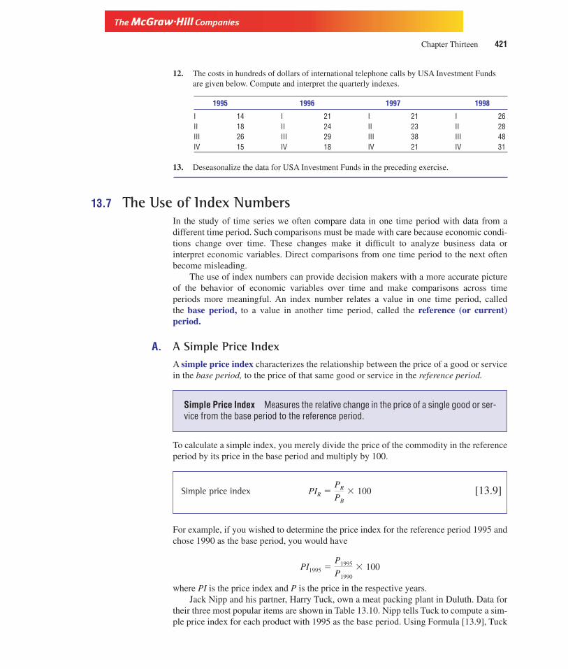
Version, Third Edition
12. The costs in hundreds of dollars of international telephone calls by USA Investment Fundsare given below. Compute and interpret the quarterly indexes.
1995 1996 1997 1998
I 14 I 21 I 21 I 26II 18 II 24 II 23 II 28III 26 III 29 III 38 III 48IV 15 IV 18 IV 21 IV 31
13. Deseasonalize the data for USA Investment Funds in the preceding exercise.
13.7 The Use of Index NumbersIn the study of time series we often compare data in one time period with data from adifferent time period. Such comparisons must be made with care because economic condi-tions change over time. These changes make it difficult to analyze business data orinterpret economic variables. Direct comparisons from one time period to the next oftenbecome misleading.
The use of index numbers can provide decision makers with a more accurate pictureof the behavior of economic variables over time and make comparisons across timeperiods more meaningful. An index number relates a value in one time period, calledthe base period, to a value in another time period, called the reference (or current)period.
A. A Simple Price IndexA simple price index characterizes the relationship between the price of a good or servicein the base period, to the price of that same good or service in the reference period.
Simple Price Index Measures the relative change in the price of a single good or ser-vice from the base period to the reference period.
To calculate a simple index, you merely divide the price of the commodity in the referenceperiod by its price in the base period and multiply by 100.
Simple price index [13.9]
For example, if you wished to determine the price index for the reference period 1995 andchose 1990 as the base period, you would have
where PI is the price index and P is the price in the respective years.Jack Nipp and his partner, Harry Tuck, own a meat packing plant in Duluth. Data for
their three most popular items are shown in Table 13.10. Nipp tells Tuck to compute a sim-ple price index for each product with 1995 as the base period. Using Formula [13.9], Tuck
PI1995 �P1995
P1990
� 100
PIR �PR
PB
� 100
Chapter Thirteen 421

Version, Third Edition
finds that the price indexes for beef in each of the three years are
From the base year of 1995 to 1996, the price index rose from 100 to 110. Tuck cantherefore conclude that the price of beef increased by 10 percent. This is calculated as thedifference between the two index numbers divided by the base number. That is,
Similarly, it can be concluded that a 50 percent increase occurred from 1995 to 1997:
You might want to conclude that a 40 percent increase in price occurred from 1996 to1997 since the price index increased by 40. However, this is not the case. The percentageincrease from 1996 to 1997 is
The 40 percent difference between the index numbers in 1996 and 1997 is called the per-centage point increase, not the percentage increase.
Notice that the price index in the base year is always 100. This will always be the casesince the price in the base year is, of course, 100 percent of itself.
The indexes for pork and veal are calculated in similar fashion and are shown inTable 13.11. Notice that the 1997 index for veal is less than 100. This reflects the fact thatveal prices in 1997 were lower than they were in the base year of 1995. Specifically, pricesfor veal went down by (100 � 91)�100 � 9 percent from 1995 to 1997.
� 36.4%
PI1997 � PI1996
PI1996
�150 � 110
100
� 50%
�PI199
P7
I
�
199
P
5
I1995� � �
150
1
�
00
100�
� 10%
�PI199
P6
I
�
199
P
5
I1995� � �
110
1
�
00
100�
� 150
PI1997 �P1997
P1995
� 100 �3.00
3.00� 100
� 110
PI1996 �P1996
P1995
� 100 �3.00
3.00� 100
� 100
PI1995 �P1995
P1995
� 100 �3.00
3.00� 100
422 Time Series and Index Numbers
Table 13.10Data for Nipp andTuck, Inc.
Price/Unit
Item Unit 1995 1996 1997
Beef 1 pound 3.00 3.30 4.50Pork 1 pound 2.00 2.20 2.10Veal 1 pound 4.00 4.50 3.64

Version, Third Edition
Example 13.5 Monthly prices for a gallon of gasoline are shown here. Using March as the base period,calculate the price indexes. What were the percentage increases, from March to May, andfrom May to June? What is the percentage point increase from May to June?
Jan Feb Mar Apr May June July
1.79 1.82 1.96 2.01 2.10 2.25 2.15
Solution:Price Indexes (March = 100)
Month Index Month Index
Jan (100) � 91.3 May (100) � 107.1
Feb (100) � 92.9 June (100) � 114.8
March (100) � 100 July (100) � 109.7
Apr (100) � 102.6
The percentage increase from March to May is
From May to June, the percentage increase is
and the percentage point increase is 114.8 � 107.1 � 7.7%
Interpretation: The base period will always report an index of 100. Periods in which the values are lessthan the base year will have an index less than 100, and periods with values in excess ofthat in the base year will have an index above 100.
B. Composite Price IndexesOften we want to calculate a price index for several goods. This is called a compositeprice index. Firms that produce two or more products are usually interested in a compos-ite index. So are many government agencies that chart consumer behavior. The U.S.
114.8 � 107.1
107.1� 7.2%
107.1 � 100.0
100.0� 7.1%
2.01�1.96
2.15�1.96
1.96�1.96
2.25�1.96
1.82�1.96
2.10�1.96
1.79�1.96
Chapter Thirteen 423
Table 13.11Price Indexes forNipp and Tuck, Inc.(1995 � 100)
Item 1995 1996 1997
Beef � 100 � 100 � 100 � 110 � 100 � 150
Pork � 100 � 100 � 100 � 110 � 100 � 105
Veal � 100 � 100 � 100 � 112 � 100 � 913.64�4.00
4.50�4.00
4.00�4.00
2.10�2.00
2.20�2.00
2.00�2.00
4.50�3.00
3.30�3.00
3.00�3.00

Version, Third Edition
Department of Labor compiles the Consumer Price Index, which measures relative pricesfor a typcal “market basket” of goods and services consumed by the general public.
The composite index is computed by adding the price of the individual commoditiesin the reference year and dividing by the summation of those prices in the base year. Theresult is then multiplied by 100.
Composite price index [13.10]
Using the data for Nipp and Tuck, we find that the 1995 composite index for all three prod-ucts, retaining 1995 as the base period, is
The index for 1996 is
PI1996 � (100) � 111.1
And 1997 produces
This means that in 1997 it would take $113.80 to buy what $100 would buy in 1995.
C. Weighted Composite Price IndexesAt least two problems arise with the use of composite price indexes. The first concerns thearbitrary way in which the units are expressed. Had Nipp and Tuck priced beef at $1.50 perhalf-pound instead of $3.00 per pound, the price index would have been entirely different.Second, the composite indexes as computed do not take into account the fact that somegoods sell in larger quantities than do other, less popular, products. No consideration isgiven to the respective amounts of each product that are sold.
For example, the composite index calculated for Nipp and Tuck gives the same im-portance, or weight, to beef as to pork, even though twice as much of the former may havebeen purchased by the consumers. It is for these reasons that we may want to compute aweighted price index. Such a calculation assigns different weights to individual prices.These weights are established so as to measure the amounts sold of each product. Thisprovides a more accurate reflection of the true cost of the consumer’s market basket ofgoods.
The quantities selected as weights can be taken from the number of units sold in (1) thebase period or (2) the reference period. Two common indexes are the Laspeyres index andthe Paasche index. The Laspeyres index uses quantities sold in the base year as weights; thePaasche index relies on quantities sold in the reference year as weights. Each procedure hasits own advantages and disadvantages.
The Laspeyres index uses base period weights (quantities) in its calculation. Therationale is that these quantities will not change from one calculation to the next, therebypermitting more meaningful comparisons over time.
PI1997 �4.50 � 2.10 � 3.64
3.00 � 2.00 � 4.00(100) � 113.8
3.30 � 2.20 � 4.50���3.00 � 2.00 � 4.00
PI1995 �3.00 � 2.00 � 4.00
3.00 � 2.00 � 4.00(100) � 100.0
PIR ��PR
�PB
� 100
424 Time Series and Index Numbers

Version, Third Edition
Laspeyres Index A weighted composite price index that uses quantities sold in thebase period as the weight factor.
To illustrate, consider the data for Nipp and Tuck in Table 13.12, which also includesthe amounts sold for each product. The Laspeyres index is
Laspeyres index [13.11]
where PR is the price in the reference period, and PB and QB are the price and quantities soldin the period selected as the base period.
L ��(PR � QB)�(PB � QB)
� 100
Chapter Thirteen 425
Table 13.12Nipp and Tuck, Inc.
Price/Unit Quantity Sold (100’s lb)
Item Unit 1995 1996 1997 1995 1996 1997
Beef 1 pound 3.00 3.30 4.50 250 320 350Pork 1 pound 2.00 2.20 2.10 150 200 225Veal 1 pound 4.00 4.50 3.64 80 90 70
The numerator uses QB, the quantities of each item in the base year. Table 13.13 showsthe computations necessary for the Laspeyres index using 1995 as the base year. The nu-merator for L is figured by first multiplying each price by the quantities sold in the baseperiod of 1995. The denominator is then determined by multiplying the price in the base yearby the quantity in the base year. The index for 1995
The index for 1996 uses the prices in the reference year (1996) and the quantities in thebase year (1995) for the numerator:
� 110.58
�1,515
1,370(100)
L1996 ��(P1996 � Q1995)�(P1995 � Q1995)
(100)
�1,370
1,370(100) � 100
L1995 ��(P1995 � Q1995)�(P1995 � Q1995)
(100)
Table 13.13The Laspeyres Indexfor Nipp and Tuck(1995 � 100)
PriceQuantities
PR 3 QB
Item 1995 1996 1997 in 1995 P95Q95 P96Q95 P97Q95
Beef 3.00 3.30 4.50 250 750 825 1,125.0Pork 2.00 2.20 2.10 150 300 330 315.0Veal 4.00 4.50 3.64 80 320 360 291.2
1,370 1,515 1,731.2

Version, Third Edition
The numerator for 1997 uses prices in 1997 and quantities in 1995:
The interpretation of the Laspeyres index is like that for our earlier indexes. From 1995 to1997, the price of the market basket for these three meat items increased by 26.36 percent.It would take $126.36 in 1997 to buy what $100 did in 1995. Or, alternatively, it would re-quire $1.26 in 1997 to buy what $1.00 did in 1995.
Notice that the denominator is the same in all three years: the Laspeyres index alwaysuses quantities from the base period.
The Paasche index, on the other hand, uses as weights the quantities sold in each ofthe various reference years. This has the advantage of basing the index on current con-sumer behavior patterns. As consumers change their buying habits, these changes in con-sumer tastes are reflected by the index. Commodities that no longer attract consumers’ in-terest, such as buggy whips and top hats, do not receive as much consideration. However,using different quantity measures makes it impossible to attribute any differences in theindex to changes in prices alone.
Paasche Index A weighted composite price index that uses quantities sold in the ref-erence period as the weight factor.
Its calculation is a bit more involved than the Laspeyres:
Paasche index [13.12]
The quantities for the reference years appear in both the numerator and the denominator.Table 13.14 provides the computation necessary for the Paasche, using the Nipp and Tuckdata with 1995 as the base. We must first multiply prices and quantities for all three yearsto get PR � QR, which is used in the numerator. We also need the value for price in the baseyear, 1995, times the quantity for each reference year to get PB � QR, which is used in the
P ��(PR � QR)�(PB � QR)
� 100
� 126.36
�1,731.2
1,370(100)
L1997 ��(P1997 � Q1995)�(P1995 � Q1995)
(100)
426 Time Series and Index Numbers
Table 13.14Paasche Index forNipp and Tuck(1995 � 100)
1995 1996 1997
Item P Q P Q P Q
Beef 3.00 250 3.30 320 4.50 350Pork 2.00 150 2.20 200 2.10 225Veal 4.00 80 4.50 90 3.64 70
P95Q95 P96Q96 P97Q97 P95Q96 P95Q97
750 1,056 1,575.0 960 1,050300 440 472.5 400 450320 405 254.8 360 280
1,370 1,901 2,302.3 1,720 1,780

Version, Third Edition
denominator. The Paasche index for 1995 is
For 1996, it is
For 1997, it is
The usual interpretation applies.The Laspeyres index requires quantity data for only one year and is easier to compute.
Therefore, it is used more frequently than the Paasche. Since the base period quantities arealways used, more meaningful comparisons over time are permitted.
However, the Laspeyres tends to overweigh goods whose prices increase. This occursbecause the increase in price will decrease quantities sold, but the lower quantity will notbe reflected by the Laspeyres index because it uses quantities from the base year.
Example 13.6 The Dippy Doo Hair Salon is considering price adjustments in its services. Harriet Follicle,manager of Dippy Doo, wants to calculate Laspeyres and Paasche indexes, using these datafor prices and the number of services rendered. January is taken as the base period.
Price Quantity
Jan Feb Mar Jan Feb Mar
Shampoo $10 $12.00 $16.50 20 22 25Trim 8 10.50 9.50 25 20 25Style 12 13.50 14.00 30 31 33
Solution: The Laspeyres is based on the following table:
PriceQuantity
PR � QJan
Jan Feb Mar in Jan Jan Feb Mar
Shampoo $10 $12.00 $16.50 20 200 240.0 330.0Trim 8 10.50 9.50 25 200 262.5 237.5Style 12 13.50 14.00 30 360 405.0 420.0
760 907.5 987.5
� 100
�760
760(100)
LJan ��(PJan � QJan)�(PJan � QJan)
(100)
�2,302.3
1,780(100) � 129.3
P1995 ��(P97 � Q97)�(P95 � Q97)
(100)
�1,901
1,720(100) � 110.5
P1996 ��(P96 � Q96)�(P95 � Q96)
(100)
�1,370
1,370(100) � 100
P1995 ��(P95 � Q95)�(P95 � Q95)
(100)
Chapter Thirteen 427

Version, Third Edition
� 129.9
The Paasche index requires another set of calculations.
Jan Feb Mar
P Q P Q P Q
Shampoo 10 20 12.00 22 16.50 25
Trim 8 25 10.50 20 9.50 25Style 12 30 13.50 31 14.00 33
Price � Quantity
PJanQJan PFebQFeb PMarQMar PJanQFeb PJanQMar
200 264.0 412.5 220 250
200 210.0 237.5 160 200
360 418.5 462.0 372 396
760 892.5 1,112.0 752 846
� 118.7
Interpretation: The two indexes produce different results. They are based on different weighting systems.However, it is clear that an increase in prices by Dippy Doo is unwise. Prices have risen by29.9 percent according to the Laspeyres index and 31.4 percent according to the Paascheindex in only three months.
�1,112
846(100) � 131.4
PMar ��(PMar � QMar)�(PJan � QMar)
(100)
�892.5
752(100)
PFeb ��(PFeb � QFeb)�(PJan � QFeb)
(100)
� 100
�760
760(100)
PJan ��(PJan � QJan)�(PJan � QJan)
(100)
�987.5
760(100)
LMar ��(PMar � QJan)�(PJan � QJan)
(100)
� 119.4
�907.5
760(100)
LFeb ��(PFeb � QJan)�(PJan � QJan)
(100)
428 Time Series and Index Numbers

Version, Third Edition
As noted, the Laspeyres tends to overweigh goods whose prices rise, since this priceincrease is accompanied by a reduction in quantity that is not reflected in the Laspeyres,which uses fixed-base quantities as the weight. The Paasche, on the other hand, tends tooverweigh goods whose prices go down. In an effort to offset these shortcomings, Fisher’sideal index is sometimes suggested. This index combines the Laspeyres and the Paascheby finding the square root of their products:
The interpretation of the Fisher index is subject to some dispute. For this reason, it is notwidely used.
Table 13.15 provides a brief comparison of the advantages and disadvantages of theLaspeyres and Paasche indexes.
F � �L � P
Chapter Thirteen 429
Table 13.15Relative Advantagesand Disadvantagesof the Laspeyresand PaascheIndexes
Advantages Disadvantages
Laspeyres Requires quantity data for only one timeperiod. Thus: (1) data are obtained moreeasily, and (2) a more meaningfulcomparison over time can be made sinceany changes can be attributed to pricemovements.
Overweighs goods whose pricesincrease. Does not reflect changes inbuying patterns over time.
Paasche Reflects changes in buying habits since ituses quantity data for each referenceperiod.
Requires quantity data for each year;these data are often difficult to obtain.Since different quantities are used, it isimpossible to attribute differences inthe index to price changes alone.Overweighs goods whose prices decrease.
13.8 Specific IndexesNumerous government agencies as well as the Federal Reserve System (which is not partof the federal government) and private businesses compile different indexes for a variety ofpurposes. The use for a specific index depends on who is compiling it and what factors gointo its formulation. Perhaps the best-known index series is the consumer price index.
A. Consumer Price IndexThe consumer price index (CPI) is reported monthly by the Bureau of Labor Statistics(BLS) of the U.S. Department of Labor. It was first reported in 1914 as a means to deter-mine whether the wages of industrial workers were keeping pace with the inflation pres-sures brought on by World War I. Prior to 1978, there was only one CPI. This traditionalmeasure reflected changes in prices of a fixed market basket of about 400 goods and ser-vices commonly purchased by “typical” urban and clerical workers. It encompassed about40 percent of the nation’s total population.
In January 1978, the BLS began reporting a more comprehensive index, the consumerprice index for all urban consumers. It is called CPI-U, while the older index is CPI-W. Thenewer CPI-U covers about 80 percent of the population and includes around 3,000 con-sumer products ranging from basic necessities, such as food, clothing, and housing, toallowances for educational and entertainment expenses. In 1988 both CPI series wererebased from 1967 to 1982–1984.
Both the CPI-W and the CPI-U employ a weighting system for the types of goods andservices purchased by consumers. Food, for example, is assigned a weight, or measure ofrelative importance, of about 18, while housing is given a weight of about 43. Medical care

Version, Third Edition
and entertainment each receive a weight of 5. The total weights for all commodities sum to100. The weights on these products are adjusted about every 10 years. In this manner, theCPI-W and the CPI-U are similar to the Laspeyres index. Technically, the CPI differsslightly from a true Laspeyres because the weighting system used by the CPI is not revisedat the same time that the index is rebased. The CPI is therefore sometimes referred to as afixed-weight aggregate price index.
The CPI is highly useful in gauging inflation, measuring “real” changes in monetaryvalues by removing the impact of price changes, and to a limited extent, serving as a cost-of-living index. It is even instrumental in determining raises in Social Security benefits andnegotiated wage settlements in labor contracts. Its many uses will be more fully examinedin the next section.
B. Other IndexesThe producer price index (formerly, the wholesale price index) is also published monthlyby the BLS. It measures changes in the prices of goods in primary markets for raw materi-als used in manufacturing. It, too, is similar to the Laspeyres index and covers almost 3,000producer goods.
The industrial production index is reported by the Federal Reserve System. It is nota monetary measurement, but tracks changes in the volume of industrial output in the na-tion. The base period is currently 1977.
There are numerous stock market indexes. Perhaps the most well-known is the DowJones industrial average. This index covers 30 selected industrial stocks to represent thealmost 1,800 stocks traded in the New York Stock Exchange. Standard & Poor’s com-posite index of 500 industrial stocks is also highly watched.
13.9 Uses for the CPIMovements in the CPI have a major impact on many business conditions and economicconsiderations. As noted, the CPI is often viewed as a measure of inflation in the economy.Annual rates of inflation are measured by the percentage change in the CPI from one yearto the next. The inflation rate from year to year is
where CPIt is the CPI in time period t, and CPIt�1 is the CPI in the previous time period.
CPIt � CPIt�1
CPIt�1
� 100
430 Time Series and Index Numbers
Table 13.16CPI and InflationRates
Year CPI Inflation Rate (%) Year CPI Inflation Rate (%)
1986 109.6 1992 140.3 3.01987 113.6 3.6 1993 145.3 3.61988 118.3 4.1 1994 148.2 1.91989 124.3 5.1 1995 152.4 2.81990 127.2 2.3 1996 156.9 3.01991 136.2 7.1 1997 158.6 1.1
Table 13.16 shows the CPI for 1986 to 1997 using 1982–1984 as the base. The figureswere taken from the Federal Reserve Bulletin, published monthly by the Board of

Version, Third Edition
Governors of the Federal Reserve System. The inflation rate for 1987, for example, is
Changes in the CPI are also often taken as a measure of the cost of living. It is argued,however, that such a practice is questionable. The CPI does not reflect certain costs or ex-penditures such as taxes, nor does it account for changes in the quality of goods available.Further, the CPI fails to measure other valued items in our economic structure, such as in-creased leisure time by the average worker or improvements in the variety of commoditiesfrom which consumers can choose. Nevertheless, the CPI is often cited in the popular pressas a measure of the cost of living.
The CPI is often the basis for adjustments in wage rates, Social Security payments, andeven rental and lease agreements. Many labor contracts contain cost-of-living adjustments(COLAs) which stipulate that an increase in the CPI of an agreed-upon amount will auto-matically trigger a rise in the workers’ wage levels.
The CPI can also be used to deflate a time series. Deflating a series removes theeffect of price changes and expresses the series in constant dollars. Economists oftendistinguish between nominal (or current) dollars and real (or constant) dollars. If a timeseries, such as your annual income over several years, is expressed in terms of 1982 dol-lars, that income is said to be real income. Assume your money (nominal) income was asshown in Table 13.17. In 1994, for example, you actually earned $42,110. It would seemthat you are doing quite well financially. Your income increased from $42,110 to $53,500over that time period. However, prices have been going up also. To obtain a measure ofhow much your income has really increased, in real terms, you must deflate your incomestream. This is done by dividing your money income by the CPI and multiplying by 100.The result is your real income expressed in constant (real) dollars of a given base year.
113.6 � 109.6
109.6(100) � 3.6%
Chapter Thirteen 431
Table 13.17Money and RealIncomes forSelected Years
Money CPI RealYear Income (1982–84 = 100) Income
1994 $42,110 148.2 28,4141995 46,000 152.4 30,1831996 49,800 156.9 31,7391997 53,500 158.6 33,732
Real Income The purchasing power of money income.
You earned $42,110 in 1994, but, as seen in Table 13.17, it was worth only $28,414 in1982–1984 prices. That is, keeping prices constant at the 1982–1984 level, you are earningan equivalent of only $28,414.
Economists commonly deflate gross national product (GNP) to obtain a measurementof the increase in our nation’s real output. Gross national product is the monetary valueof all final goods and services produced in our economy. By deflating GNP over time, econ-omists eliminate any increase due to price inflation, and arrive at a measure of the actual in-crease in the production of goods and services available for consumption.
Real income �Money income
CPI� 100
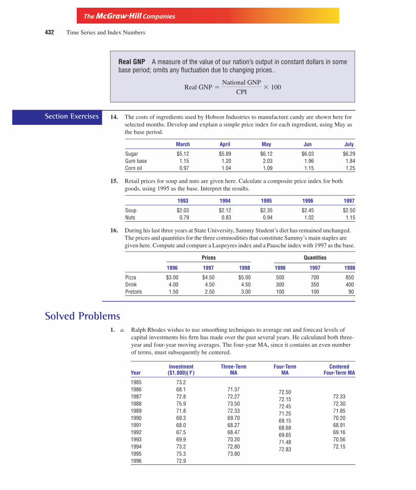
Version, Third Edition
Real GNP A measure of the value of our nation’s output in constant dollars in somebase period; omits any fluctuation due to changing prices..
14. The costs of ingredients used by Hobson Industries to manufacture candy are shown here forselected months. Develop and explain a simple price index for each ingredient, using May asthe base period.
March April May Jun July
Sugar $5.12 $5.89 $6.12 $6.03 $6.29Gum base 1.15 1.20 2.03 1.96 1.84Corn oil 0.97 1.04 1.09 1.15 1.25
15. Retail prices for soup and nuts are given here. Calculate a composite price index for bothgoods, using 1995 as the base. Interpret the results.
1993 1994 1995 1996 1997
Soup $2.03 $2.12 $2.35 $2.45 $2.50Nuts 0.79 0.83 0.94 1.02 1.15
16. During his last three years at State University, Sammy Student’s diet has remained unchanged.The prices and quantities for the three commodities that constitute Sammy’s main staples aregiven here. Compute and compare a Laspeyres index and a Paasche index with 1997 as the base.
Prices Quantities
1996 1997 1998 1996 1997 1998
Pizza $3.00 $4.50 $5.00 500 700 850Drink 4.00 4.50 4.50 300 350 400Pretzels 1.50 2.50 3.00 100 100 90
Solved Problems1. a. Ralph Rhodes wishes to use smoothing techniques to average out and forecast levels of
capital investments his firm has made over the past several years. He calculated both three-year and four-year moving averages. The four-year MA, since it contains an even numberof terms, must subsequently be centered.
Investment Three-Term Four-Term CenteredYear ($1,000)(Y ) MA MA Four-Term MA
1985 73.21986 68.1 71.37 72.501987 72.8 72.27 72.15 72.331988 75.9 73.50 72.45 72.301989 71.8 72.33 71.25 71.851990 69.3 69.70 69.15 70.201991 68.0 68.27 68.68 68.911992 67.5 68.47 69.65 69.161993 69.9 70.20 71.48 70.561994 73.2 72.80 72.83 72.151995 75.3 73.801996 72.9
Real GNP �National GNP
CPI� 100
432 Time Series and Index Numbers
Section Exercises

Version, Third Edition
Using the three-term MA, 73.8 is the estimate of the long-run average around which all ob-servations tend to fall and, as such, is the forecast for any future time period. The four-termMA produces an estimate of 72.15.
2. For the past several years, business conditions for Rainbow Enterprises have been rather black.The CEO has collected quarterly totals of the number of employees who have been laid offover the past four years.
a. The CEO would like to forecast the number of layoffs for the first and second quarters of1998, using linear trend analysis.
Time Layoffs (Y ) t (X ) XY X 2
1994-I 25 1 25 1II 27 2 54 4III 32 3 96 9IV 29 4 116 16
1995-I 28 5 140 25II 32 6 192 36III 34 7 238 49IV 38 8 304 64
1996-I 35 9 315 81II 37 10 370 100III 37 11 407 121IV 39 12 468 114
1997-I 38 13 494 169II 42 14 588 196III 44 15 660 225IV 45 16 720 256
562 136 5,187 1,496
� 35.13 � 1.206(8.5)
For the first quarter of 1998,
� 45.38
Yt � 24.88 � 1.206(17)
� 24.88
b0 � Y � b1X
� 1.206
b1 �410
340
� 410
� 5,187 �(136)(562)
16
SSxy � �XY �(�X)(�Y)
n
� 340
� 1,496 �(136)2
16
SSx � �X 2 �(�X)2
n
Chapter Thirteen 433

Version, Third Edition
for the second quarter of 1998,
b. The CEO now wants to develop the seasonal indexes for the number of layoffs.
Time Layoffs Centered MA Ratio to MA
1994-I 25II 27III 32 28.625 1.1179IV 29 29.625 0.9789
1995-I 28 30.500 0.9180II 32 31.875 1.0039III 34 33.875 1.0037IV 38 35.375 1.0742
1996-I 35 36.375 0.9622II 37 36.875 1.0034III 37 37.375 0.9900IV 39 38.375 1.0163
1997-I 38 39.875 0.9530II 42 41.500 1.0120III 44IV 45
The four-term (since quarterly data are used) MA is calculated and centered, followed bythe ratio to MA. The mean ratio to MA is then determined for each quarter. Since themeans sum to 4.0111, the normalization ratio is 4�4.011 � 0.999. The seasonal indexes areobtained by multiplying each mean ratio to MA by 0.997.
1994 1995 1996 1997 Mean Seasonal Indexes
I 0.9180 0.9622 0.9530 0.9444 0.9416II 1.0039 1.0034 1.0120 1.0064 1.0034III 1.1179 1.0037 0.9900 1.0372 1.0341IV 0.9789 1.0742 1.0163 1.0231 1.0200
4.0111 3.9991 � 4
c. The CEO for Rainbow wants to determine layoffs if the seasonal factors are eliminated.Deseasonalized levels of layoffs for 1994-I and 1994-II are, respectively,
and
d. Rainbow executives think that general movements in the business cycle influence theirneed to lay off employees. They decide to calculate the cyclical components for each timeperiod.
27
1.0034� 26.91 employees
25
0.9416� 26.55 employees
� 46.59
Yt � 24.88 � 1.206(18)
434 Time Series and Index Numbers

Version, Third Edition
(1) (3) (4) (5) (6) (7)Time (2) Trend Seasonal Statistical Cyclical- Cyclical
Period Layoffs Projection Index Norm Irregular Component
1994-I 25 26.08 0.9416 24.56 101.80II 27 27.29 1.0034 27.38 98.61III 32 28.49 1.0341 29.46 108.62 100.5IV 29 29.70 1.0200 30.29 95.73 99.61
1995-I 28 30.90 0.9416 29.10 96.24 98.73II 32 32.11 1.0034 32.22 99.32 99.01III 34 33.32 1.0341 34.46 98.68 101.51IV 38 34.52 1.0200 35.21 107.92 102.55
1996-I 35 35.73 0.9416 33.64 104.03 102.01II 37 36.93 1.0034 37.06 99.85 100.06III 37 38.14 1.0341 39.44 93.81 98.15IV 39 39.35 1.0200 40.14 97.17 97.64
1997-I 38 40.55 0.9416 38.18 99.52 98.34II 42 41.76 1.0034 41.90 100.23 99.33III 44 42.96 1.0341 44.42 99.04IV 45 44.17 1.0200 45.05 99.88
They take a four-term MA of the cyclical-irregular values to produce just the cyclical com-ponent in column (7). For 1994-III, the layoff of 32 employees represents 100.5 percent ofthe trend.
e. If layoffs in 1998-I are 46, what might Rainbow expect total layoffs for 1998 to be? Sincethe first quarter typically repreents a period in which layoffs are only 94.16 percent of theaverage for the full year, quarterly layoffs based on 46 for 1998-I would be
For the whole year, layoffs would total (48.85)(4) � 195 employees.f. In a final effort to control the number of necessary layoffs, Rainbow executives wish to ob-
tain deseasonalized figures for each time period. They obtain these by dividing the actualnumber of layoffs by the appropriate seasonal (quarterly) index. A partial listing of the re-sults is shown.
Seasonal DeseasonalizedYear-Quarter Layoffs Index Layoffs
1994-IV 25 0.9416 26.55II 27 1.0034 26.91III 32 1.0341 30.94IV 29 1.0200 28.43
1995-I 28 0.9416 29.74
3. The Laspeyres and Paasche Indexes Your firm manufactures three grades of lubricant. Theprices and quantities sold for each are as follows:
Prices Quantities
Grade Oct Nov Dec Oct Nov Dec
A $3.00 $3.30 $4.00 250 320 350B 2.00 2.10 2.10 150 200 225C 4.00 4.50 3.64 80 90 70
46
0.9416� 48.85
Chapter Thirteen 435
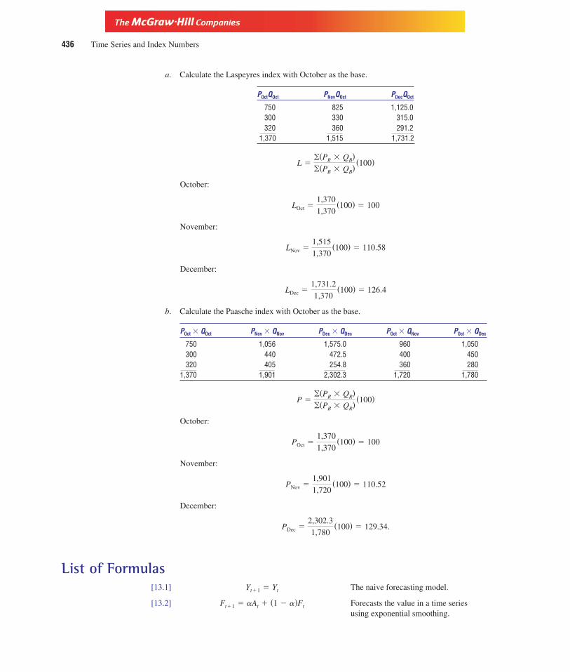
Version, Third Edition
a. Calculate the Laspeyres index with October as the base.
POctQOct PNovQOct PDecQOct
750 825 1,125.0300 330 315.0320 360 291.2
1,370 1,515 1,731.2
October:
November:
December:
b. Calculate the Paasche index with October as the base.
POct 3 QOct PNov 3 QNov PDec 3 QDec POct 3 QNov POct 3 QDec
750 1,056 1,575.0 960 1,050300 440 472.5 400 450320 405 254.8 360 280
1,370 1,901 2,302.3 1,720 1,780
October:
November:
December:
.
List of Formulas[13.1] The naive forecasting model.
[13.2] Forecasts the value in a time seriesusing exponential smoothing.
Ft�1 � aAt � (1 � a)Ft
Yt�1 � Yt
PDec �2,302.3
1,780(100) � 129.34
PNov �1,901
1,720(100) � 110.52
POct �1,370
1,370(100) � 100
P ��(PR � QR)�(PB � QR)
(100)
LDec �1,731.2
1,370(100) � 126.4
LNov �1,515
1,370(100) � 110.58
LOct �1,370
1,370(100) � 100
L ��(PR � QB)�(PB � QB)
(100)
436 Time Series and Index Numbers

Version, Third Edition
[13.3] Calculates the mean square error.
[13.4] Estimate for the trend line.
[13.5]Sums of squares of X used to computethe trend line.
[13.6]Sums of the cross-products of X and Yused to compute the trend line.
[13.7] Computes the slope of the trend line.
[13.8] Computes the intercept of the trend line.
[13.9]A simple price index; measures the rela-tive change in the price of a single goodor service from the base period to thereference period.
[13.10]A composite price index; calculates theindex for several goods or services.
[13.11]The Laspeyres index uses the quantitiesin the base year as weights.
[13.12]The Paasche index uses quantities in thereference year as weights.
Chapter Exercises17. Cars-R-Us has recorded sales (in $1,000s) over the last three years of
Month 1996 1997 1998 Month 1996 1997 1998
Jan 17.2 18.1 16.3 July 24.2 23.9 22.7Feb 18.7 19.2 17.3 Aug 25.7 26.2 25.0March 19.7 20.3 18.5 Sep 21.2 22.0 21.9April 20.2 21.5 20.3 Oct 19.3 18.0 17.3May 21.7 22.0 21.0 Nov 22.7 19.7 21.2June 23.1 24.7 25.0 Dec 19.3 17.3 16.2
a. Plot the data. Does there appear to be any trend in the data? Any cyclical or seasonalvariation?
b. Compute a 12-month moving average. Which component or components do these valuesreflect?
18. Calculate the seasonal indexes for each month using the data for Cars-R-Us from the previousexercise.
19. In Exercise 17, what are the seasonally adjusted sales figures for the last six months of 1998?How do you interpret them?
20. In Exercise 17, what are the deseasonalized values for the last six months of 1998? Howwould you interpret them?
P ��(PR � QR)�(PB � QR)
(100)
L ��(PR � QB)�(PB � QB)
(100)
PIR ��PR
�PB
(100)
PIR �PR
PB
� 100
b0 � Y � b1X
b1 �SSxy
SSx
SSxy � �XY �(�X)(�Y)
n
SSx � �X 2 �(�X)2
n
Yt � b0 � b1t
MSE ��(Ft � At)
2
n � 1
Chapter Thirteen 437

Version, Third Edition
21. Business Monthly recently reported the dollar value of “perks” received by business execu-tives over the past several years. These data do not include that portion of the executives’health care paid by the employer, and are adjusted for inflation. Use linear trend analysis topredict the value for the year 2000. How well does the model explain the trend in perklevels?
Year Perk Year Perk
1980 $3,200 1989 $4,2801981 3,640 1990 4,4501982 3,850 1991 4,5001983 3,700 1992 4,4901984 3,920 1993 4,5601985 3,880 1994 4,6801986 3,950 1995 4,7901987 4,1001988 4,150
22. Inventories for Bake-O-Donuts for the past two years were
Month 1995 1996 Month 1995 1996
Jan $ 87 $ 95 July $ 80 $83Feb 93 102 Aug 73 79March 102 112 Sep 93 84April 112 115 Oct 102 89May 93 99 Nov 115 92June 82 90 Dec 112 91
a. Use a 12-period moving average to remove seasonal variations.b. Calculate the seasonal indexes.c. What are the seasonally adjusted inventory levels?
23. Mopeds, Inc., is concerned about slumping sales. If monthly sales fall below $9,000 theNortheast regional office must be closed down. According to the figures shown here, is thatlikely to occur within the next five months? Figures are in thousands.
1996
J F M A M J J A S O N D
18 17.3 16.9 18.1 16.8 16.3 15.1 14.5 14 14.5 14 13.1
1997
13.9 13.1 12.8 12.4 11.8 11.9 11.7 11.5 11.1 11.2 11.2 11.1
24. Using the data from the previous exercise, calculate the seasonal indexes.
25. Using the data for Mopeds, Inc., what is the strength of the relationship between sales andtime? Plot the trend line against the actual data.
26. From the regression model you calculated in the exercise for Mopeds, Inc., what is the aver-age monthly change in sales?
27. John Wolf feels that exponential smoothing with an a-value of 0.8 can best forecast Septem-ber inventories of his medical supply firm. His brother and business partner thinks an a of 0.4should be used. What is the forecast in each case? Who is correct, based on the values shown
438 Time Series and Index Numbers

Version, Third Edition
below for inventories per month?
Inventories J F M A M J J A
($100) 41 48 37 32 45 43 49 38
28. Three Finger Louis, the town’s only butcher, is concerned about the volume of customers’ baddebt he must write off as uncollectable each month. Dollar amounts in hundreds are shownhere for the past three years.
1995
14.1 13.7 12.1 13.1 13.5 9.1 7.2 6.1 8.7 10.1 11.8 12.2
1996
15.2 14.1 13.2 13.9 14.0 9.5 7.2 6.5 9.1 11.5 12.2 13.4
1997
13.7 12.5 11.8 12.0 13.0 8.7 6.3 6.0 8.2 9.8 10.9 11.8
a. Plot the data. Does a seasonal factor seem to exist? (Consider a “season” to be onemonth.)
b. Use a 12-month moving average to smooth out the seasonal variation.c. Calculate seasonal indexes.d. Deseasonalize the data.e. Plot the original data and the deseasonalized data.
29. Packer Industries is concerned that sales may fall below $100,000 in December. Using thedata shown below in thousands of dollars, what is your projection? Plot the data first.
Jan Feb Mar Apr May June July Aug
42.7 57.3 68.3 76.8 84 88.1 90 90.1
30. U.S. News & World Report stated that projections by the U.S. Department of Commerce formedian earnings of full-time workers were
Year Earnings ($1,000) Year Earnings ($1,000)
1990 24.28 2020 90.941995 30.26 2025 113.332000 37.71 2030 171.232005 47.00 2035 176.002010 58.56 2040 219.332015 73.00
a. Plot the data.b. Compute the trend model.c. What is the projection for the year 2050?
31. Milles Products recorded the profits shown in the table.
a. Use exponential smoothing to forecast future profits. First, set a � 0.2,then 0.9.
b. Which a-value produces a more reliable estimate?
Chapter Thirteen 439

Version, Third Edition
c. How could you have known this beforehand?
Week 1 2 3 4 5 6 7Profits ($1,000) 10 25 3 15 2 27 5
32. Consumer data supplied by the U.S. Department of Commerce for the summer of 1998 revealed the following:
Prices
Unit 1996 1997 1998
Beef 1 pound $3.12 $3.89 $3.92Milk 1 gallon 2.10 2.42 2.51Chicken 1 pound 1.95 2.10 2.12Bread 1 loaf 0.99 0.89 1.12
Compute and interpret the simple index for each commodity using 1996 as the baseperiod.
33. Given the data from the previous problem, compute
a. The percentage increase in the price of each product for1996 to 1997.1996 to 1998.1997 to 1998.
b. The percentage point increase for each product for1996 to 1997.1996 to 1998.1997 to 1998.
34. Below are costs for a one-day stay in the hospital. Use 1993 as the base year and compute thesimple index. Interpret the index obtained for 1990.
1990 1991 1992 1993 1994 1995
$356 $408 $512 $589 $656 $689
35. Sammy Studd wants to purchase an entire new wardrobe of athletic wear for the summer. Hehas collected the data shown below and wonders how prices have changed over the past threeyears. Compute and interpret the composite price index for all four goods, using 1996 as thebase year.
1996 1997 1998
Shoes $89.90 $115.12 $125.00Sweats 52.50 65.50 75.50Shorts 25.75 35.95 45.90Socks 12.10 10.00 9.50
36. Prices for a new line of toy dolls by The Krazy Kid Kollection are shown below. Using1994–1995 as the base period, calculate a simple price index for all three toys.
1994 1995 1996
Killer Joe $17.90 $21.50 $25.00Pyro Phil 15.00 25.00 29.95Maniac Mark 10.00 11.00 12.00
440 Time Series and Index Numbers

Version, Third Edition
37. Bell electronic wishes to analyze price changes for three of its products over the past threeyears. The necessary data are given here.
Prices Quantities
Product 1996 1997 1998 1996 1997 1998
A $10.00 $15.50 $20.00 150 170 160B 3.00 5.00 7.50 55 68 120C 69.00 75.00 75.00 100 90 85
38. Compute and interpret the Laspeyres and Paasche indexes using 1996 as the base period.Using the data from the previous exercise, compute the Fisher index.
39. Pam McGuire, the director of operations for Columbia Records, compiled the following dataon recording costs and the number of times each item was used over the last three years forthree items commonly used in the recording business.
Cost per Usage Usage Frequency
1996 1997 1998 1996 1997 1998
Studio costs $120 $145 $165 30 35 37Recording equipment 420 530 620 40 43 46Backup singers 300 250 250 50 63 72
Sam O’Donnell, the director of statistical procedures, must calculate a Laspeyres index anda Paasche index, using 1996 as the base, and must then determine the rate at which costshave risen each year under both indexes, as well as the rate of inflation over all threeyears.
40. From Exercise 39, which index is probably a better measure of Columbia’s rise in costs?Why? Support your choice.
41. Just Pizza bought the amounts of ingredients at the prices shown in the table below. JanetJackson, manager of Just Pizza, is worried about rising prices. Develop Laspeyres andPaasche indexes for her, using January as the base.
Price/Pound Pounds Used (100’s)
Jan Feb Mar Apr Jan Feb Mar Apr
Cheese 2.10 2.15 2.20 2.25 10 12 15 12Pepperoni 1.18 1.20 1.25 1.31 8 10 8 10Sausage 1.25 1.31 1.35 1.42 7 6 7 7
42. Using Janet’s data from the previous exercise, does the Paasche index show that the rate atwhich prices are going up is increasing or decreasing?
Computer ExerciseSpark Industries has been suffering a noticeable drop in profits over the past several years. While theprice of its product has remained fairly stable, the number of employees necessary to maintain pro-duction has shown a pronounced upward trend, causing labor costs to rise dramatically.
To curb this undesirable trend, you have been charged with the responsibility of analyzingSpark’s price levels and number of employees. Access the file SPARK on your data disk. It contains
Chapter Thirteen 441

Version, Third Edition
50 observations of quarterly data for the retail price of their product (PRICE) and for the number ofemployees (EMPL).
You must use smoothing techniques to forecast future prices and provide a complete decompo-sition of the time series data for employees. Prepare your findings in a statistical report as describedin Appendix I.
442 Time Series and Index Numbers
C U R T A I N C A L LIn Setting the Stage at theopening of this chapter,we noted how Mr. Dickson
uses statistical analysis in making businessdecisions. As owner and chief executive of-ficer, he places considerable importance oncareful planning and the timing of his oper-ations.
Mr. Dickson has hired you as an out-side statistical consultant to provide himwith valuable information about his busi-ness that he feels will prove highly useful informulating future plans. Specifically, yourtask is to predict profits using a four-periodmoving average based on the data below.
Further, you are to compare this projectionto that obtained through exponential smooth-ing. Mr. Dickson has not specified an alphavalue for the smoothing constant and ex-pects you to determine what value is optimal.
Finally, the sales of the firm are also ofconcern to Mr. Dickson. Given the data pro-vided here, you must develop and interpret atrend line as well as decompose the time se-ries by breaking out each component indi-vidually. Present your final report to Mr.Dickson in the form of a statistical report asdescribed in Appendix I. Include all relevantresults as well as your interpretation.
Time Profits Revenues Time Profits RevenuesPeriod ($00) ($000) Period ($00) ($000)
1995-I 25 10 1997-I 32 25II 29 12 II 28 20III 24 15 III 33 26IV 28 14 IV 31 32
1996-I 31 17 1998-I 24 34II 27 19 II 35 38III 24 17 III 28 41IV 28 21 IV 25 45
From the Stage to Real LifeMr. Dickson, the industrial business owner of the Setting the Stage chapter opening, be-lieves that changes in the overall economic climate affect the values of his profits and salesrevenues. In fact, he would be able to investigate the extent that the general economy af-fects the value of his profits by adjusting them for changes in the overall price level, usingthe CPI (consumer price index) published by the U.S. Department of Labor. He also is ableto compare his sales levels to both the GDP (gross domestic product) and the final sales ofall U.S. finished goods, using indexes published by the U.S. Department of Commerce.
These indexes are available on the Internet. To locate the CPI data, go to the statisticslocation of the Department of Labor (http://stats.bls.gov:80/ ). Once there, choose the“Data” area. Then click on “Most Requested Series.” At the next page, click on “OverallMost Requested Series.” The following page allows you to select the index, the years cov-

Version, Third Edition
ered, and the data delivery format you desire. Scroll down to the heading “Price Indexes”and choose CPI for All Urban Consumers 1982–1984 � 100. Further down this page,choose the years for your analysis, say 1987–1997. Last, on this same page, select the Tableof your choice under the “Format” heading. This completes your request for data. Clickingon “Retrieve” produces the CPI data of interest to you.
GDP and Final sales of goods are found at the Department of Commerce site(http://www.doc.gov/ ). At the home page, click on “Commerce Web Sites (arranged by bu-reau).” Next, click on the “Bureau of Economic Analysis” (BEA). Then choose the BEAdata area. Click on “National.” Scroll down to the heading “Historical time series” andclick on “Tables.” Here you can choose to click on either “GDP and final sales, Annually”or “GDP and final sales, Quarterly” for the data of your interest.
Chapter Thirteen 443

Version, Third Edition
444
C H A P T E R14Chi-Square and OtherNonparametric Tests

Version, Third Edition
445
Chi-Square and Other Nonparametric Tests
A uniform distribution
A specific pattern
A normal distribution
Signs test
Runs test
Mann-Whitney test
Spearman rank correlation
Kruskal-Wallis test
Other nonparametric tests
Goodness-of-fit
A test for independence
Chi-square
Chapter BlueprintMany of the tests we performed in previous chapters required certain basic assumptions before thetest could be carried out. We assumed that the population was normally distributed or that variancesfit particular patterns. When those assumptions cannot be made, or essential knowledge about thepopulation is not attainable, we have to rely on the nonparametric tests contained in this chapter.
Version, Third Edition
14.1 IntroductionPrevious chapters presented many tests for hypotheses. We performed tests for both popu-lation means and population proportions. In some instances the sample size was greaterthan 30, whereas in others the sample was small. We examined tests for a single populationand tests comparing two or more populations.
However, all these test situations exhibited one common characteristic: they requiredcertain assumptions regarding the population. For example, t-tests and F-tests required theassumption that the population was normally distributed. Since such tests depend on pos-tulates about the population and its parameters, they are called parametric tests.
In practice, many situations arise in which it is simply not possible to safely make anyassumptions about the value of a parameter or the shape of the population distribution.Most of the tests described in earlier chapters would therefore not be applicable. We mustinstead use other tests that do not depend on a single type of distribution or specific para-metric values. These are called nonparametric (or distribution-free) tests. This chapterexamines several of these statistical tools.
446 Chi-Square and Other Nonparametric Tests
S E T T I N G T H E S T A G EFor many years Mama’sPizzeria has been a popu-lar hangout for students at
the nearby university. This year, however,Mama has faced vigorous competition fromDante’s, a new business that opened on theother side of the campus. Dante’s offers anextensive menu that attracts many studentseager to sample the new fare.
Mama has decided that she must ex-pand her selection or lose customers to theinterloper who has intruded into the marketthat before had been exclusively hers. Mamarecognizes this will require many delicatedecisions that can be made only after carefulconsideration of the consequences.
In order to make these decisions,Mama has hired you as her statistical assis-tant to analyze the market, evaluate the al-ternatives, and devise a plan to regain herprominence as the major provider of stu-dents’ staple needs. You realize this impor-tant assignment will require the full extentof your statistical expertise.
Mama has agreed to pay you in foodand drink for the rest of the semester if you
can help her. Spurred by this generous offer,you are determined to provide Mama withthe best possible advice.
After careful thought, you determinewhat data you must collect, how they mustbe organized, and precisely what tests youmust run to provide Mama with the infor-
mation she needs to make some pressing de-cisions. You are also aware that the assump-tions needed to carry out the statistical testsyou have studied so far are not valid and thatthis task will require you to rely on the non-parametric tests covered in this chapter.

Version, Third Edition
Nonparametric Tests Statistical procedures that can be used to test hypotheseswhen no assumptions regarding parameters or population distributions are possible.
14.2 Chi-Square Distribution (x2)One of the more useful nonparametric tools is the chi-square (x2) test. Like the t-distribu-tion, the chi-square distribution is an entire family of distributions. There is a different chi-square distribution for each degree of freedom. Figure 14.1 shows that as the number of de-grees of freedom increases, the chi-square distribution becomes less skewed. The two mostcommon applications of chi-square are (1) goodness-of-fit tests and (2) tests for indepen-dence. We will examine each in turn.
Chapter Fourteen 447
df = 1
df = 5
df = 10
f ( 2)χ
2χ
Figure 14.1The Chi-SquareDistribution
A. Goodness-of-Fit TestsBusiness decisions often require that we test some hypothesis about the unknown popula-tion distribution. We might, for instance, hypothesize that the population distribution isuniform and that all possible values have the same probability of occurring. The hypothe-ses that we would test are
H0: The population distribution is uniform.
HA: The population distribution is not uniform.
The goodness-of-fit test is then used to determine whether the distribution of values in thepopulation fits a particular hypothesized shape—in this case, a uniform distribution. Aswith all the statistical tests of this nature, sample data are taken from the population andthese form the foundation for our findings.
Goodness-of-Fit Tests Measures of how closely observed sample data fit a particu-lar hypothesized distribution. If the fit is reasonably close, it may be concluded that thehypothesized distribution exists.

Version, Third Edition
If there is a large difference between what is actually observed in the sample and whatyou would expect to observe if the null hypothesis were correct, then it is less likely thatthe null is true. That is, the null hypothesis must be rejected when the observations obtainedin the sample differ significantly from the pattern that is expected to occur if the hypothe-sized distribution does exist.
For example, if a fair die is rolled, it is reasonable to hypothesize a pattern in the out-comes such that each outcome (numbers 1 through 6) occurs approximately one-sixth ofthe time. However, if a significantly large or significantly small percentage of even num-bers occurs, it may be concluded that the die is not properly balanced and that the hypoth-esis is false. That is, if the difference between the pattern of events actually observed andthe pattern of events expected to occur if the null is correct proves too great to attribute tosampling error, it must be concluded that the population exhibits a distribution other thanthat specified in the null hypothesis.
To test the hypothesis regarding a population distribution, we must analyze the dif-ference between our expectations based on the hypothesized distribution and the actualdata occurring in the sample. This is precisely what the chi-square goodness-of-fit testdoes. It determines if the sample observations “fit” our expectations. The test takes theform
Chi-square test [14.1]
where Oi is the frequency of observed events in the sample dataEi is the frequency of expected events if the null is correctK is the number of categories or classes
The test carries K � m � 1 degrees of freedom, where m is the number of parametersto be estimated. The exact impact of m will become more apparent as our discussion pro-gresses.
Notice that the numerator of Formula [14.1] measures the difference between the fre-quencies of the observed events and the frequencies of the expected events. When thesedifferences are large, causing �2 to rise, the null should be rejected.
1. A test for a Uniform Fit Chris Columbus, marketing director for Seven Seas, Inc., has theresponsibility of controlling the inventory level for four types of sailboats sold by his firm.In the past he has ordered new boats on the premise that all four types are equally popularand the demand for each type is the same. Recently, however, inventories have becomemore difficult to control, and Chris feels that he should test his hypothesis regarding a uni-form demand. His hypotheses are
H0: Demand is uniform for all four types of boats.
HA: Demand is not uniform for all four types of boats.
By assuming uniformity in demand, the null hypothesis presumes that out of a randomsample of sailboats, weekend sailors would purchase an equal number of each type. To testthis hypothesis, Chris selects a sample of n � 48 boats sold over the past several months.If demand is uniform, he can expect that 48�4 � 12 boats of each type were sold. Table 14.1shows this expectation, along with the number of each type that actually was sold. Noticethat �(Oi) � �(Ei). Chris must now determine whether the numbers actually sold in each
x 2 � �K
i�1
(Oi � Ei)2
Ei
448 Chi-Square and Other Nonparametric Tests

Version, Third Edition
of the K � 4 categories are close enough to what he would expect if demand was uniform.Formula [14.1] gives
The value 1.17 is then compared with a critical x 2-value taken from Table H inAppendix III.Since there were no parameters that had to be estimated, m � 0 and there are K � 1 � 3degrees of freedom. If Chris wanted to test at the 5 percent level, he would find, as shownin Figure 14.2, that
Decision Rule Do not reject if x2 # 7.815. Reject if x2 . 7.815.
Since 1.17 , 7.815, the null hypothesis that demand is uniform is not rejected. The dif-ferences between what was actually observed, Oi, and what Chris would expect to ob-serve if demand was the same for all four types of sailboats, Ei, are not large enough torefute the null. The differences are not significant and can be attributed merely to sam-pling error.
Minitab can be used to perform the calculations. Merely input the data for the ob-served frequencies in the first column and the data for the expected frequencies in thesecond column. In the session window, type
MTB> LET K1 = SUM((C1 - C2)**2/C2)MTB> PRINT K1.
The first line tells Minitab to calculate Formula [14.1]. The second line tells Minitab toreport back the chi-square statistic. Using the data for Chris’ boats, the value of 1.16667 isreturned.
x 20.05,3 � 7.815.
� 1.17
x 2 �(15 � 12)2
12�
(11 � 12)2
12�
(10 � 12)2
12�
(12 � 12)2
12
Chapter Fourteen 449
Table 14.1Seven Seas SalesRecord
Type Observed Sales Expected Salesof Boat (Oi) (Ei)
Pirates’ Revenge 15 12Jolly Roger 11 12Bluebeard’s Treasure 10 12Ahab’s Quest 12 12
48 48
f ( 2)χ
1.17 7.815
0.05
2χ
Figure 14.2A Chi-Square Testfor Seven Seas

Version, Third Edition
The p-value for the test is the area to the right of our sample findings of 1.17 as seen inFigure 14.2. We can see only that it is greater than 5 percent. Minitab will also compute thep-value by
MTB> CDF K1 K2;SUBC> CHISQUARE 1.MTB> LET K3 = 1 - K2MTB> PRINT K3.
Minitab will return the p-value of 0.280087.
2. A Test for a Fit to a Specific Pattern In our example regarding the sailboats, Chris assumedthat the demand for all four types of sailboats was the same. The values for the expectedfrequencies were therefore all the same. However, many instances arise in which frequen-cies are tested against a certain pattern in which expected frequencies are not all the same.Instead, they must be determined as
Expected frequencies [14.2]
where n is the sample sizepi is the probability of each category as specified in the null hypothesis
Example 14.1 demonstrates.
Example 14.1 The John Dillinger First National Bank in New York City tries to follow a policy of ex-tending 60 percent of its loans to business firms, 10 percent to individuals, and 30 percentto foreign borrowers.
To determine whether this policy is being followed, Jay Hoover, vice-president ofmarketing, randomly selects 85 loans that were recently approved. He finds that 62 of thoseloans were extended to businesses, 10 to individuals, and 13 to foreign borrowers. At the10 percent level, does it appear the bank’s desired portfolio pattern is being preserved? Testthe hypothesis that
H0: The desired pattern is maintained: 60 percent are business loans, 10 percentare individual loans, and 30 percent are foreign loans.
HA: The desired pattern is not maintained.
Solution: If the null hypothesis is correct, Mr. Hoover would expect 60 percent of the 85 loans in thesample to be business loans. So, for the first category, Ei � npi � (85)(0.60) � 51 loans tobusinesses. In addition, he would expect that (85)(0.10) � 8.5 of the loans would be toindividuals, and (85)(0.30) � 25.5 loans to foreign customers. The data are summarizedin the table.
Type of Observed Frequencies Expected FrequenciesLoan (Oi) (Ei)
Business 62 51.0Private 10 8.5Foreign 13 25.5
85 85.0
Ei � npi
450 Chi-Square and Other Nonparametric Tests

Version, Third Edition
The x2-value is
Again, no parameters were estimated and m � 0. With a set at 10 percent and K � 3 cate-gories of loans (business, private, and foreign), there are K � m � 1 or 3 � 0 � 1 � 2degrees of freedom. Mr. Hoover finds from Table H in Appendix III that the critical
Decision Rule Do not reject the null if x2 # 4.605. Reject the null if x2 . 4.605.
As shown by the figure, the null should be rejected since 8.76 . 4.605.
x20.10,2 � 4.605.
� 8.76
x2 �(62 � 51)2
51�
(10 � 8.5)2
8.5�
(13 � 25.5)2
25.5
Chapter Fourteen 451
DNR
4.605
0.10
8.76
f ( 2)χ
2χ
Interpretation: The differences between what Mr. Hoover observed and what he would expect to observeif the desired loan pattern was achieved is too great to occur by chance. There is only a10 percent probability that a sample of 85 randomly selected loans could produce the ob-served frequencies shown here if the desired pattern in the bank’s loan portfolio wasbeing maintained.
3. A Test for Normality Specifications for the production of air tanks used in scuba divingrequire that the tanks be filled to a mean pressure of 600 pounds per square inch (psi). Astandard deviation of 10 psi is allowed. Safety allowances permit a normal distribution infill levels. You have just been hired by Aqua Lung, a major manufacturer of scuba equip-ment. Your first assignment is to determine whether fill levels fit a normal distribution.Aqua Lung is certain that the mean of 600 psi and the standard deviation of 10 psi prevail.Only the nature of the distribution remains to be tested. In this effort, you measure n �1,000 tanks and find the distribution shown in Table 14.2. Your hypotheses are
H0: Fill levels are normally distributed.
HA: Fill levels are not normally distributed.
As before, the test requires that you compare these actual observations with those youwould expect to find if normality prevailed. To determine these expected frequencies, youmust calculate the probabilities that tanks selected at random would have fill levels in theintervals shown in Table 14.2. The probability that a tank would fall in the first interval is
0

Version, Third Edition
P(0 � X � 580). The problem facing you is depicted in Figure 14.3(a). You must deter-mine the shaded area under the curve. Thus,
Then
There is slightly more than a 2 percent chance that any tank selected at random would havea fill level less than 580 psi if the mean fills are 600 psi with a standard deviation of 10 psiand are distributed normally. For the second interval, the probability that a tank selected atrandom would have a fill level between 580 and 590 is P(580 � X � 590), and is shownin Figure 14.3(b).
Then
P(580 � X � 590) � 0.4772 � 0.3413 � 0.1359
� �1, or an area of 0.3413
Z2 �590 � 600
10
� �2, or an area of 0.4772
Z1 �580 � 600
10
P(0 � X � 580) � 0.5000 � 0.4772 � 0.0228
� �2, or an area of 0.4772
Z �580 � 600
10
Z �X � m
s
452 Chi-Square and Other Nonparametric Tests
Table 14.2Fill Levels for ScubaTanks
ActualPSI Frequency
0 and under 580 20580 and under 590 142590 and under 600 310600 and under 610 370610 and under 620 128620 and above 30
1,000
0.4772
600
(a)
580 psi 580
0.34130.13
59
600
(b)
590
0.4772
psi0.0228
0.0228 0.4772
Figure 14.3 Probabilities of Tank Fills

Version, Third Edition
The probabilities for the remaining intervals are calculated in like fashion and are shown inTable 14.3, along with the expected frequencies. The expected frequencies, as before, areEi � npi. For the first interval this becomes (1,000)(0.0228) � 22.8. You wish to test the hy-pothesis at the 5 percent level. Since both the population mean and the standard deviationwere given and do not have to be estimated, m � 0. There are K � 6 classes in the frequencytable, so the degrees of freedom are K � 1 � 5.You find the critical x 2 to be x2
0.05,5 � 11.07.
Chapter Fourteen 453
Table 14.3Probabilities of FillLevels
Actual Probabilities ExpectedPSI Frequency (Oi) (pi) Frequency (Ei)
0 and under 580 20 0.0228 22.8580 and under 590 142 0.1359 135.9590 and under 600 310 0.3413 341.3600 and under 610 370 0.3413 341.3610 and under 620 128 0.1359 135.9620 and above 30 0.0228 22.8
1,000 1.0000 1000.0
Decision Rule Do not reject the null if x2 is less than 11.07. Reject the null if x2
is greater than 11.07.
Using Formula [14.1], you find
As shown in Figure 14.4, the null should not be rejected. The differences between whatwere observed and what you would expect to observe if the fills were normally distributedwith a mean of 600 and a standard deviation of 10 can be attributed to sampling error.
Had the population mean and standard deviation not been known, we would have hadto estimate them from the sample data in Table 14.2. Then m would be 2, and the degreesof freedom would be K � 2 � 1 or 6 � 2 � 1 � 3.
Caution: The chi-square test for goodness-of-fit is reliable only if all Ei are at least 5.If a class has an Ei � 5, it must be combined with adjacent classes to ensure that all Ei �5. Had you selected a sample of only n � 100 instead of 1,000 scuba tanks, the Ei for thefirst class would have been Ei � npi � (100)(0.0228) � 2.28 instead of 22.8. This firstclass would be combined with the second class so that Ei � 5. Similarly, class 6 would
� 8.63
x2 �(20 � 22.8)2
21.5�
(142 � 135.9)2
135.9� ≥ �
(30 � 22.8)2
21.5
2
f ( 2)
11.07
0.05
8.63
DNR
χ
χ
Figure 14.4Chi-Square Test forNormality

Version, Third Edition
have an Ei � 2.28 and would be combined with class 5. Of course, the degrees of freedomare reduced accordingly.
What would happen if you set the first class at “570 and under 580” and the last one at“620 and under 630” to keep all intervals equal? Very little. The P(Xi) would not quite equal1, and �(Ei) would not quite equal �(Oi). However, it would be entirely possible to do so.
Again, Minitab will produce the desired results. Minitab Display 14.1 contains theinput commands and the resulting output. The p-value is 0.00329876 � 0.05, leading tothe rejection of the null.
Minitab Display 14.1
MTB > let k1 = sum((c1 - c2)**2/c2) [Calculates the chi-square value]MTB > print k1
Data Display
K1 8.63444 [The chi-square value]MTB > cdf k1 k2;SUBC> chisquare 1. )Calculates the p-value*MTB > let k3 = 1 - k2 MTB > print k3
Data Display
K3 0.00329876 [The p-value]MTB >
B. Contingency Tables—A Test for IndependenceNotice that in all the problems so far, there was one and only one factor that captured ourinterest. However, chi-square will also permit the comparison of two attributes to deter-mine whether there is a relationship between them. A retailer may want to discover whetherthere is a connection between consumers’ income levels and their preference for his prod-uct. Production managers are always concerned about any relationship that might exist be-tween the productivity of their employees and the type or degree of training they received.
Wilma Keeto is the director of product research at Dow Chemical. In her current pro-ject Ms. Keeto must determine whether there is any relationship between the effectivenessrating consumers assign to a new insecticide and the location (urban or rural) in which it isused. Of the 100 consumers surveyed, 75 lived in urban areas and 25 in rural areas. Table 14.4summarizes the ratings by each consumer in a contingency table like those discussed inChapter 4.
The table has r � 3 rows and c � 2 columns. There are rc � 6 cells in the table. No-tice, for example, that 31 customers rated the product “above average”; 20 of those were inurban areas.
454 Chi-Square and Other Nonparametric Tests
Table 14.4Contingency Tablefor Dow Chemical
Attribute B—Location
Attribute A—Rating Urban Rural Total
Above average 20 11 31Average 40 8 48Below average 15 6 21
Total 75 25 100

Version, Third Edition
Ms. Keeto wants to compare attribute B (location) to attribute A (the product’s rating).Her hypotheses are
H0: Rating and location are independent.
HA: Rating and location are not independent.
If location has no impact on effectiveness rating, then the percentage of urban resi-dents who rated the product “above average” should equal the percentage of rural residentswho rated the product “above average.” This percentage in turn should equal that of allusers who rated the product “above average.”
As shown in Table 14.4 above, 31 percent of all 100 users rated the product “above av-erage.” Then 31 percent of the 75 urban residents and 31 percent of the 25 rural residentsshould also give this rating if rating and location are independent. These values of(75)(0.31) � 23.3 and (25)(0.31) � 7.75 give the expected frequencies Ei for each cell, asshown in Table 14.5.
Chapter Fourteen 455
Table 14.5Rating Frequencies
Attribute B
Attribute A Urban Rural Totals
Oi � 20 Oi � 11 31Above average Ei � 23.3 Ei � 7.75
Oi � 40 Oi � 8 48Average Ei � 36 Ei � 12
Oi � 15 Oi � 6 21Below average Ei � 15.8 Ei � 5.25
Total 75 25 100
The remaining Ei are calculated in similar fashion and displayed in Table 14.5. For ex-ample, 48 percent of the 100 users rated the product as “average.” Therefore, if the null iscorrect, 48 percent of the 75 urban customers should also rate the product “average,” and48 percent of the 25 rural consumers should record a rating of “average.” The Ei are calcu-lated as (75)(0.48) � 36 and (25)(0.48) � 12. Similarly, since 21 of the 100 users, or 21 per-cent, rated the product “below average,” then 21 percent of the 75 people living in urbancenters (Ei � 15.8) and 21 percent of the 25 living in rural areas (Ei � 5.25) should providea “below average” rating.
Testing the hypothesis requires a comparison of Oi and Ei over the rc � 6 cells, usingthe equation
Chi-square test [14.3]
For the current problem, Wilma finds
� 3.76
�(8 � 12)2
12�
(15 � 15.8)2
15.8�
(6 � 5.25)2
5.25
x 2 �(20 � 23.3)2
23.3�
(11 � 7.75)2
7.75�
(40 � 36)2
36
x 2 � �rc
i�1
(Oi � Ei)2
Ei

Version, Third Edition
The test carries (r � 1)(c � 1) � (3 � 1)(2 � 1) � 2 degrees of freedom. If Wilmaset a � 10 percent, As Figure 14.5 shows, the null is not rejected accord-ing to the decision rule:
Decision Rule Do not reject the null if x2 # 4.605. Reject if x2 . 4.605.
Minitab Display 14.2 is obtained by placing the data for urban customers in column 1and those for rural residents in column 2 and then clicking on STAT > TABLES >CHISQUARE TEST.
Minitab Display 14.2Chi-Square Test
Expected counts are printed below observed counts
C1 C2 Total1 20 11 A 31 The top number in each cell is Oi.
23.25 7.75 A The bottom number is Ei.
2 40 8 4836.00 12.00
3 15 6 2115.75 5.25
Total 75 25 100
Chisq = 0.454 + 1.363 +0.444 + 1.333 +0.036 + 0.107 = 3.738
df = 2, p = 0.155
Notice that the chi-square value of 3.738 and the p-value of 0.155 are reported.Example 14.2 provides further illustration.
Example 14.2 Hedonistic Auto Sales sets out to determine whether there is any relationship betweenincome of customers and the importance they attach to the price of luxury automobiles.The company’s managers want to test the hypotheses that
H0: Income and importance of price are independent.
HA: Income and importance of price are not independent.
x20.10,2 � 4.605.
456 Chi-Square and Other Nonparametric Tests
2
f ( 2)
DNR
4.6053.76
0.10
χ
χ
Figure 14.5Chi-Square Test ofIndependence

Version, Third Edition
Solution: Customers are grouped into three income levels and asked to assign a level of significanceto price in the purchase decision. Results are shown in the contingency table. Since 182�538� 33.83 percent of all respondents attach a “great” level of importance to price, then, if in-come and price are not related, we would expect 33.83 percent of those in each incomebracket to respond that price was of “great” importance. Thus, the Ei for a “low” level of im-portance are (198) (0.3383) � 66.98, (191)(0.3383) � 64.62, and (149)(0.3383) � 50.41.
Attribute A:Attribute B: Income
Importance Level Low Medium High Total
Great Oi � 83 Oi � 62 Oi � 37 182Ei � 66.98 Ei � 64.62 Ei � 50.41
Moderate Oi � 52 Oi � 71 Oi � 49 172Ei � 63.32 Ei � 61.06 Ei � 47.64
Little Oi � 63 Oi � 58 Oi � 63 184Ei � 67.72 Ei � 65.32 Ei � 50.96
Totals 198 191 149 538
In like fashion, 172�538 � 31.97 of all respondents rated price moderately important.Thus, the Ei for the “moderate” category are 198(0.3197) � 63.32, 191(0.3197) � 61.06,and 149(0.3197) � 47.64.
For the “little” category, the data show 184�538 � 34.20 percent of all customersattached little limportance to the price. Therefore, the Ei are (198)(0.342) � 67.72, (191)(0.342) � 65.32, and (149)(0.342) � 50.96.
The chi-square is
If a is set at 1 percent, and with (r � 1)(c � 1) � (3 � 1)(3 � 1) � 4 degrees offreedom. As seen in the figure, the decision rule is
Decision Rule Do not reject the null if x2 # 13.277. Reject if x2 . 13.277.
x20.01,4 � 13.277.
� 15.17
≥ �(63 � 50.96)2
50.96
x 2 �(83 � 66.98)2
66.98�
(62 � 64.62)2
64.62�
(37 � 50.41)2
50.41�
(52 � 63.32)2
63.32�
Chapter Fourteen 457
2
f ( 2)
DNR
13.277 15.17
0.01
χ
χ
Interpretation: The null hypothesis is rejected. There is only a 1 percent chance that if there were no rela-tionship between income and price significance, the differences between Qi and Ei wouldbe great enough to produce a chi-square larger than 13.277. There is evidence of a
1
Version, Third Edition
relationship between customers’ income and the importance attached to the price of a lux-ury automobile.
The remainder of the chapter is devoted to different nonparametric tests. Several testsare examined to illustrate (1) when the test should be used, (2) the primary purpose and ap-plication of the test, and (3) the interpretation of the test. We explore the
Sign test.
Runs test.
Mann-Whitney U test.
Spearman rank correlation test.
Kruskal-Wallis test.
We begin with the sign test.
1. The vice-president of operations at First National Bank argues that the three types of loans—auto loans, student loans, and general-purpose loans—are granted to customers in the sameproportions. To test his hypothesis, you collect data on 200 recent loans and find 55 were autoloans, 47 were student loans, and the rest were for general purposes. At the 5 percent level,what do you tell the vice-president?
2. Given the results of the previous exercise, you attest that the loans extended to customers fit apattern such that one-half are for general purposes and the rest are evenly divided between thetwo remaining types. Using the sample for the previous problem, what do you conclude at the5 percent level?
3. Shoppers at the local mall are asked to rate a new product on a continuous scale starting atzero. Based on the grouped data below, can you conclude at the 5 percent level that the dataare normally distributed, with a mean of 100 and a standard deviation of 25?
Rating Frequency
Less than 50 150–70 5170–90 11290–110 151
110–130 119130–150 43150–170 21Over 170 2
4. Analysts at Federated Stores hypothesize that the incomes of their customers are normally dis-tributed. Based on the data provided here, what conclusion do you reach at the 1 percent level?
Income ($1,000) Frequency
Less than 35 135–40 440–45 2645–50 9750–55 9655–60 6560–65 865–70 2
Above 70 1
458 Chi-Square and Other Nonparametric Tests
Section Exercises

Version, Third Edition
5. TransWorld AirWays wants to determine whether there is any relationship between the numberof flights people take and their income. What conclusion do you reach at the 1 percent levelbased on the data for 100 travelers in the contingency table?
Frequency of Flights
Income Never Seldom Often
Less than $30,000 20 15 2$30,000–50,000 8 5 1$50,000–70,000 7 8 12
Over $70,000 2 5 15
14.3 Sign TestA nonparametric test commonly used to make business decisions is the sign test. It is mostoften used to test the hypothesis comparing two population distributions, and often in-volves the use of matched pairs. Suppose we have before-and-after data for a sample andwish to compare these matched sets of data. We do it by subtracting the paired observationsin one data set from those in the second, and noting the algebraic sign that results. We haveno interest in the magnitude of the difference, only whether a plus sign or a minus signresults.
The sign test is the nonparametric counterpart to the t-test for matched pairs. The t-testrequired the assumption that the populations were normally distributed. In many instances,this assumption is not possible. The sign test is useful in these cases.
The null hypothesis states that there is no difference in the data sets. If this is true, thena plus sign and a minus sign are equally likely. The probability that either would occur is0.50. A two-tailed test is
where m and p are the numbers of minus signs and plus signs, respectively. A one-tailedtest is
or
Sign Test A test designed to test the hypothesis comparing the distributions of twopopulations.
Since there are only two possible outcomes, a minus sign and a plus sign, and the prob-ability of each remains constant from trial to trial, we can use the binomial distribution.
Assume you are working as a market analyst and wish to measure the effectivenessof a promotional game on your firm’s product. Prior to the promotional game, you select12 retail outlets and record sales for the month, rounded to the nearest $100. During the
HA: m � p
H0: m � p
HA: m p
H0: m p
HA: m � p
H0: m � p
Chapter Fourteen 459

Version, Third Edition
second month, the promotional game is implemented and you again record sales. Table 14.6displays these sales levels, along with the algebraic sign that results when sales in the sec-ond month are subtracted from those in the first month. A plus sign recorded in the last col-umn means that sales went down during the second month.
Assume further that you want to test at the 5 percent level the hypothesis that the pro-motion increased sales. If sales went up in the second month when the promotion was in ef-fect, then subtracting those sales from sales in the first month would produce minus signs.You would then expect the number of minus signs, m, to exceed the number of plus signs,p. That is, m . p. This statement does not contain an equal sign and is, therefore, the al-ternative hypothesis, producing a right-tailed test:
You must now ask, “What would cause the null to be rejected?” Since the null states thatm # p, then either (1) a significantly large number of minus signs or (2) a significantlysmall number of plus signs would result in the rejection of the null. That is, the null is re-jected if m is too large or if p is too small.
Table 14.6 shows 6 minus signs and 4 plus signs for a total of n � 10 signs. Values re-sulting in a zero difference are ignored. Observations 3 and 9 are therefore dropped fromconsideration. You must then determine the probability of six or more minus signs or fouror fewer plus signs if the probabilities of both are p � 0.50. If this probability is less thanthe chosen a-value, the sample results are significant and the null hypothesis is rejected.However, if the probability of the sample results is greater then a, the results can be attrib-uted to sampling error; do not reject the null. That is, if the sample results actually observedare likely to occur, they are not interpreted as being a significant finding and the null can-not be rejected.
From Table C in Appendix III, the probability of six or more minus signs is
Of course, if you obtained six or more minus signs, you must have obtained four or fewerplus signs. Therefore, the probability of four or fewer plus signs is also 0.3770:
P(p 4}n � 10, p � 0.5) � 0.3770
� 0.3770
� 1 � 0.6230
P(m � 6}n � 10, p � 0.5) � 1 � P(X 5)
HA: m p
H0: m p
460 Chi-Square and Other Nonparametric Tests
Table 14.6Sales for TwelveRetail Stores
Before DuringStore the Game the Game Sign
1 $42 $40 �
2 57 60 �
3 38 38 04 49 47 �
5 63 65 �
6 36 39 �
7 48 49 �
8 58 50 �
9 47 47 010 51 52 �
11 83 72 �
12 27 33 �

Version, Third Edition
This value of 0.3770 is the probability of obtaining six or more minus signs (or fouror fewer plus signs) if p, the probability of the occurrence of either sign on any trial, is0.50. We noted that if the number of minus signs was unusually large, it would refute thenull. However, 6 is not an unusually large number. The probability of getting six or moresigns is quite high at 37.7 percent. Since the probability of their occurrence is greater thanan a of 5 percent, the event of six minus signs is not considered large, and the null thatH0: m $ p is not rejected.
If the promotion were effective, there would be a large number of minus signs, and thenull that m # p would be rejected. But as we have seen, six minus signs is not an unusu-ally large number, and you cannot consider the promotion successful.
If a test were based on the left-tailed test, the hypothesis would be
If m is unusually small, or p is unusually large, the null would be rejected. Assume thatan experiment with n � 12 trials yields five minus signs and seven plus signs. You wouldthen find the probability of obtaining five or less minus signs, or the probability of seven ormore plus signs. If this probability is less than the chosen a, reject the null.
Example 14.3 illustrates a two-tailed test. The only adjustment is that a must be di-vided by 2. The hypotheses are
The hypotheses are tested by comparing a�2 to either (1) the probability that the sign thatoccurred less often could occur that many times or less, or (2) the probability that the signthat occurred more often could occur that many times or more.
Example 14.3 Honda tested the wear resistance of two types of tire tread on its Nighthawk motorbike. Tenbikes were randomly chosen. Mechanics mounted tires with one type of tread on the front,and the other tread on the rear. After driving the bikes a specified number of miles under setconditions, they gave a wear rating between 0 and 40 to each tire. A higher rating indicateda better tire. The results are shown here. Honda’s research analysts want to test the hypoth-esis that there is no difference in wear ratings at the 10 percent level. The hypotheses are
Wear Rating
Tires Tread Type I Tread Type II Sign
1 32 37 �
2 27 25 �
3 21 21 04 13 17 �
5 25 29 �
6 38 39 �
7 17 23 �
8 29 33 �
9 32 34 �
10 34 37 �
HA: m � p
H0: m � p
HA: m � p
H0: m � p
HA: m � p
H0: m � p
Chapter Fourteen 461

Version, Third Edition
Solution: Observation 3 is ignored because the difference is zero. There is one plus sign and eightminus signs. Honda can calculate the probability that one or fewer plus signs could occuror the probability that eight or more minus signs could occur. Focusing on the number ofplus signs, we have, from Table C (Appendix III),
Of course, we get the same answer if we use the number of minus signs is the test:
Since a�2 � 0.10�2 � 0.05 0.0195, the null is rejected.
Interpretation: If the null is true, and m � p, there is only a 1.95 percent chance of getting one or fewerplus signs (or eight or more minus signs). There is a less than a�2 � 0.05 percent chancethat the null is true. We can conclude that there is a difference in wear ratings. Tread type IIis superior since there was a significant number of minus signs.
If n $ 30, it is permissible to use the normal approximation to the binomial. Assumethat in the preceding example, Honda had sampled 40 motorbikes and obtained 8 plussigns, 28 minus signs, and 4 zero differences. The company would have n � 36 useful ob-servations.
As we learned in Chapter 8, if the test is two-tailed with a � 0.10, the critical Z-valueis 1.65.
Decision Rule Do not reject if �1.65 Ztest 1.65. Reject if Ztest � �1.65 orZtest 1.65.
The value for Ztest is
Z-value for largesample sign test [14.4]
where k is the appropriate number of plus or minus signs and n is the sample size. Ifk � n�2, k � 0.5 is used. If k n�2, k � 0.5 is used. It is necessary to adjust k by 0.5because the binomial distribution represents discrete data, while the normal distributionapplies to continuous data.
Since the Honda example is a two-tailed test, we can test either the number of plussigns or the number of minus signs. Testing the number of plus signs, we have
Testing the number of minus signs, we find
� 3.17
Ztest �28 � 0.5 � (0.5)(36)
0.5�36
� �3.17
Ztest �8 � 0.5 � (0.5)(36)
0.5�36
Ztest �k � 0.5 � 0.5n
0.5�n
P(m � 8}n � 9, p � 0.5) � 1 � P(m 7) � 1 � 0.9805 � 0.0195
P(p 1}n � 9, p � 0.5) � 0.0195
462 Chi-Square and Other Nonparametric Tests
Version, Third Edition
Since �3.17 � �1.65, or 3.17 1.65, the null is rejected. There is a difference in the twotypes of tires. Trend type II is superior.
6. Two advertisements for computers are rated by 15 potential customers to determine whether apreference exists. The results are shown here. At the 10 percent level, what are the results?
Consumer 1 2 3 4 5 6 7 8 9 10 11 12 13 14 15
Ad 1 8 9 5 7 9 4 3 8 9 5 7 8 8 7 9Ad 2 7 3 2 8 5 5 7 2 1 3 7 2 2 3 8
7. The manufacturer of 10 snack foods hypothesizes that the sales of each product with a highfat content will be less than those of the same product with reduced fat. Sales in thousands ofunits are given below. At the 10 percent level, what is your conclusion?
Food 1 2 3 4 5 6 7 8 9 10
With fat 10 12 14 18 17 18 5 21 6 8Without fat 15 13 12 9 17 19 3 27 12 14
8. The brilliance of glassware is measured on a scale from 1 to 100. Twenty glasses are tested be-fore and after being treated by a new process. If subtracting the brilliance factor after treatmentfrom that before treatment results in 5 plus signs and 3 negative signs, is there any differenceat the 5 percent level? How do you interpret the results of the test?
9. Fifty employees who have received special training are matched with 50 others who are simi-lar in every aspect but did not receive the training. The productivity of those who were trainedis subtracted from that of those who were not trained, resulting in 15 plus signs and 17 nega-tive signs. At the 5 percent level, did the training make a difference?
14.4 Runs TestThe importance of randomness in the sampling process has been repeatedly stressed. In theabsence of randomness, many of the statistical tools upon which we rely are of little or nouse. It is therefore often necessary to test for randomness in our samples. We can accom-plish this using a runs test.
Runs Test A nonparametric test for randomness in the sampling process.
To complete a runs test, we assign all observations in the sample one of two symbols.A run consists of a sequence of one or more like symbols. If the observations are groupedinto categories of, say, A and B, we might find the following sequences:
AA BBB A BB AAA B
1 2 3 4 5 6
There are six runs, each consisting of one or more like observations.
Run An unbroken series of one or more like symbols.
Chapter Fourteen 463
Section Exercises

Version, Third Edition
Suppose employees are selected for a training program. If selection does not dependon whether the employee is male (m) or female (f), we would expect gender to be a randomevent. However, if some pattern in gender is detected, we might assume randomness is ab-sent and selection was made at least in part on the basis of a worker’s gender. If there is anunusually large or an unusually small number of runs, a pattern is suggested.
Assume that the gender of each employee is recorded in order of selection and provesto be
mmm ffffff mmm
1 2 3
Three runs occur in this sample. There are three males, followed by six females, and thenthree males. It would seem that the selections are not sufficiently mixed, causing a system-atic pattern which implies an absence of randomness. Assume instead that the order ofselection is
m f m f m f m f m f m f
1 2 3 4 5 6 7 8 9 10 11 12
Again, there appears to be a pattern producing an unusually large number of 12 separateruns.
Detection of a Pattern If too few or too many runs occur, randomness may beabsent.
The set of hypotheses to be tested is
H0: Randomness exists in the sample.
HA: Randomness does not exist in the sample.
To test the hypothesis, we must determine whether the number of runs (r) is either too largeor too small. Table M1 and M2 (Appendix III), show critical values for the number of runsif a is 5 percent. Since on the surface both of our examples appear nonrandom, let’s take aless obvious set of selections. Suppose the selections were
m fff mmm ff mmm
1 2 3 4 5
The selections seem more random than the other two examples in that no pattern is obvi-ous. Notice that n1 � 7 is the number of males and n2 � 5 is the number of females.
Table M1 shows the minimum critical number of runs for an a-value of 5 percent. Ifthe number of runs is equal to or less than the value shown in Table M1, it suggests that,at the 5 percent level, there are too few runs to support the null hypothesis of random-ness. Given that n1 � 7 and n2 � 5, we find the critically low value to be 3. Since thenumber of runs exceeds this minimum, there is not a significantly low number of runs towarrant rejection of the null. Table M2 provides critically high values for r. If the num-ber of runs in a sample is equal to or greater than those values, we may conclude thatthere is an extremely large number of runs, suggesting the absence of randomness. For
464 Chi-Square and Other Nonparametric Tests

Version, Third Edition
n1 � 7 and n2 � 5, Table M2 reveals that the maximum number of runs is 11. If the num-ber of runs exceeds 11, there are too many to support the hypothesis of randomness.Since the number of runs is less than 11, it is not significantly high and the null is notrejected at the 5 percent level. It would seem that our sample selection is the result ofrandomness.
When the sample data do not naturally fall into one of two possible categories, it ispossible to use the median as a measure to bifurcate the data. Assume levels of daily out-put at a coal mine selected for a statistical study are, in order of selection, 31, 57, 52, 22,24, 59, 25, 29, 27, 44, 43, 32, 40, 37, 60 tons. The median of 37 can be used as a bench-mark value. Observations fall either above (A) or below (B) 37, yielding eight runs of
31 57 52 22 24 59 25 29 27 44 43 32 40 60
B AA BB A BBB AA B AA
1 2 3 4 5 6 7 8
With n1 � 7 for B and n2 � 7 for A, Table M reveals critical values of 3 and 13 runs. Sincethere were eight runs, randomness is assumed and the null is not rejected.
Another application of the runs test is found in a test of randomness in the ordinaryleast squares (OLS) method of regression analysis. A basic property of the OLS regressionmodel is that the errors are random. No pattern should exist in the signs of these errors.Example 14.4, illustrates how the runs test can be used to test this condition.
Example 14.4 A marketing research firm developed a model to predict monthly sales for a new product.After 17 months, the errors were calculated and proved to have the following signs:
� � � � � � �
1 2 3 4
At the 5 percent level, does there appear to be randomness in the error terms?
Solution: There are n1 � 10 plus signs, n2 � 7 minus signs, and r � 4 runs. Tables M1 and M2 re-veal the critical minimum and maximum numbers of runs, respectively, to be 5 and 14. Thehypotheses are
H0: Randomness prevails.
HA: Randomness does not prevail.
Decision Rule Do not reject the null if 5 � r � 14. Reject if r 5 or r � 14.
Since r � 4, the null should be rejected at the 5 percent level.
Interpretation: The number of runs is significantly small. There are too few runs to support the hypothesisof randomness. The validity of the regression model is questionable, and the firm shouldexamine alternatives. The low number of runs results from the fact that errors of one signare followed by errors of like signs, an indication of positive autocorrelation.
Chapter Fourteen 465

Version, Third Edition
If both n1 and n2 are greater than 20, the sampling distribution for r approximates nor-mality. The distribution has a mean of
Mean of the samplingdistribution of the number [14.5]of runs
and a standard deviation of
Standard deviationfor runs test [14.6]
Standardizing the distribution of runs can be accomplished by using the normal deviate:
Normal deviate fordistribution of runs [14.7]
A sales presentation made to a group of 52 potential buyers resulted in 27 sales, 25 no-sales, and 18 runs. At the 1 percent level of significance, is the sample random?
H0: The sample is random.
HA: The sample is not random.
At 1 percent, the critical Z for the two-tailed test is 2.58. As shown in Figure 14.6, the de-cision rule is
Z �r � mr
sr
sr � � 2n1n2(2n1n2 � n1 � n2)(n1 � n2)
2(n1 � n2 � 1)
mr �2n1n2
n1 � n2
� 1
466 Chi-Square and Other Nonparametric Tests
–2.58 0 Z2.58–2.52
0.005 0.005
DNR
Figure 14.6Testing forRandomness inSales
Decision Rule Do not reject the null if �2.58 Z 2.58. Reject the null ifZ � �2.58 or Z 2.58.
Then, by Formula [14.5],
� 26.96
�2(27)(25)27 � 25
� 1
mr �2n1n2
n1 � n2
� 1

Version, Third Edition
and, by Formula [14.6],
The normal deviate is
There is insufficient evidence to reject the null. It would appear that the sample is random.There is a 99 percent probability that a random sampling process with 27 and 25 observa-tions in the two categories, and with 18 runs, would lead to a Z between �2.58.
Example 14.4 can be used to illustrate how Minitab can perform a runs test. In column1 of the data window, enter six 1’s for the 6 plus signs, five 2’s for the 5 minus signs, four1’s for the next four plus signs, and then two 2’s for the last two minus signs. Click onSTAT > NONPARAMETRICS > RUNS TEST. Select Above and Below and enter 1.5.Click OK. The printout is shown as Minitab Display 14.3. The p-value tells us that the nullis rejected at any alpha value above 0.0068.
Minitab Display 14.3Runs Test
C1
K = 1.5000
The observed no. of runs = 4The expected no. of runs = 9.23537 Observations above K 10 below
* N Small -- Following approx. may be invalidThe test is significant at 0.0068
14.5 Mann-Whitney U TestThe Mann-Whitney U test (or simply the U test) tests the equality of two population dis-tributions. It is based on the assumption that two random samples are independently drawnfrom continuous variables. In its broadest sense, the null hypothesis states that the distrib-utions of two populations are identical. However, the test can be tailored to examine theequality of two population means or medians. To test the equality of means, we must as-sume that the populations are symmetrical and have the same variance. Under these condi-tions the Mann-Whitney U test serves as the nonparametric alternative to the t-test, except
� �2.52
�18 � 26.96
3.56
Z �r � mr
sr
� 3.56
� �[2(27)(25)][2(27)(25) � 27 � 25](27 � 25)2(27 � 25 � 1)
sr � � 2n1n2(2n1n2 � n1 � n2)(n1 � n2)
2(n1 � n2 � 1)
Chapter Fourteen 467

Version, Third Edition
it does not require the assumption of normality. If the assumption of symmetry is dropped,the median replaces the mean as the test statistic.
Mann-Whitney U Test The nonparametric counterpart to the t-test for independentsamples. It does not require the assumption that the differences between the two sam-ples are normally distributed.
The data are ordered or ranked from lowest to highest. There is no effort to matchpairs, as we have often done when two samples were taken. (Note that the Mann-WhitneyU test is the same as the Wilcoxon rank sum test, but differs from the Wilcoxon signed-ranktest. The similarity in names can be confusing.)
To illustrate the U test, suppose a pottery factory wants to compare the time it takes forclay pieces to cool after being “fired” in the oven by two different firing methods.
Potters fire 12 pieces using method 1, and 10 using method 2. The number of minutesrequired for each piece to cool is as follows:
Method 1: 27* 31 28 29 39 40 35 33 32 36 37 43Method 2: 34 24* 38 28 30 34 37 42 41 44
The observations are then ordered and ranked from lowest to highest as shown in Table 14.7.The value 24 in method 2 is the lowest of all 22 observations and is given the rank of 1, and27 in method 1 has a rank of 2. Ties, such as 28, are averaged over the appropriate ranks.The value 28 is the third lowest observation, and both values of 28 receive a ranking of 3.5.There is no rank of 4, since two observations have the rank of 3.5. The rankings are thensummed, yielding �R1 and �R2.
468 Chi-Square and Other Nonparametric Tests
Table 14.7Ranking CoolingTimes
Method 1 Rank Method 2 Rank
24 127 228 3.5 28 3.529 5
30 631 732 833 9
34 10.534 10.5
35 1236 1337 14.5 37 14.5
38 1639 1740 18
41 1942 20
43 2144 22
∑R1 � 130 ∑R2 � 123

Version, Third Edition
We calculate the Mann-Whitney U-statistic for each sample from the equations as
Mann-Whitney U-statisticfor first sample [14.8]
and
Mann-Whitney U-statisticfor second sample [14.9]
The data in Table 14.7 yield
and
Notice that U1 � U2 � n1n2 provides a quick check of your arithmetic.If n1 and n2 are both at least 10, the mean and standard deviation of the sampling
distribution for the U-statistic are
Mean of the samplingdistribution for Mann-Whitney U test
[14.10]
and
Standard deviation of thesampling distribution forthe Mann-Whitney U test
[14.11]
In the present case, we find
and
� 15.17
su � �(12)(10)(12 � 10 � 1)12
� 60
mu �(12)(10)
2
su � �n1n2(n1 � n2 � 1)12
mu �n1n2
2
� 52
U2 � (12)(10) �10(10 � 1)
2� 123
� 68
U1 � (12)(10) �12(12 � 1)
2� 130
U2 � n1n2 �n2(n2 � 1)
2� �R2
U1 � n1n2 �n1(n1 � 1)
2� �R1
Chapter Fourteen 469

Version, Third Edition
The distribution of the U-statistic can then be normalized by the formula
Z-value to normalizethe Mann-Whitney U test [14.12]
where Ui is the appropriate U-value, either U1 or U2, depending on the nature of the test.Let’s now determine which U-value is appropriate.
A. Two-Tailed TestIn our example of the firing ovens, the pottery factory may want to test the hypothesis thatthe mean cooling times of method 1 and method 2 are the same. This requires a two-tailedtest with hypotheses
In a two-tailed test, either U1 or U2 can be used in Formula [14.12]. Thus, arbitrarily usingU2, we find
If a � 10 percent, the decision rule, as reflected in Figure 14.7, is
� �0.53
Z �52 � 60
15.17
HA: m1 � m2
H0: m1 � m2
Z �Ui � mu
su
470 Chi-Square and Other Nonparametric Tests
–1.65 0 1.65–0.53
0.05 0.05
Z
DNR
Figure 14.7A Two-Tailed Testof Mean CoolingTimes
Decision Rule Do not reject if �1.65 Z 1.65. Reject if Z � �1.65 orZ 1.65.
Since Z � �0.53 is in the DNR region, the pottery factory can conclude at the 10 percentlevel of significance that the mean cooling times are the same for both firing methods.
B. One-Tailed TestSuppose the factory felt that method 1 would result in a longer mean cooling time: 1 2. Then the hypotheses
HA: m1 m2
H0: m1 m2

Version, Third Edition
call for a right-tailed test. If a right-tailed test is to be conducted, then the U-value in For-mula [14.12] must be the higher of the two U-values. Since U1 � 68 U2 � 52, U1 isused to calculate the Z-value. If this were a left-tailed test, the lower U-value would be usedto compute Z.
Given our right-tailed test, we have
If a = 0.10 is retained for this one-tailed test, the decision rule, as shown in Figure 14.8, is
� 0.53
Z �68 � 60
15.17
Chapter Fourteen 471
Decision Rule Do not reject if Z 1.28. Reject if Z 1.28.
The Z-value of 0.53 is clearly in the DNR region. The pottery factory does not rejectthe null hypothesis that m1 m2 and cannot conclude that method 2 leads to faster coolingtimes.
Minitab Display 14.4 shows the results of the test for the pottery factory discussedabove. Point and interval estimates for the difference in population medians are given. Thevalue of W � 130.0 is the sum of the ranks of the variable stored in the first column andcan be used to calculate U1 and U2. The p-value of 0.4057 is greater than our selected alphavalue of 10 percent and therefore tells us that we cannot reject the null.
Minitab Display 14.4Mann-Whitney Confidence Interval and Test
C1 N = 12 Median = 34.00C2 N = 11 Median = 37.00Point estimate for ETA1-ETA2 is -2.0090.9 Percent C.I. for ETA1-ETA2 is (-7.00,3.00)W = 130.0Test of ETA1 = ETA2 vs. ETA1 ~= ETA2 is significant at 0.4060The test is significant at 0.4057 (adjusted for ties)
10. The proprietor of a local pub popular with students at a nearby university was overheard tosay that female customers tended to spend less than males. Challenged to support his claimby the statistics professor occupying his usual space at the end of the bar, the pub keeper
DNR
0 0.53 1.28 Z
0.10
Figure 14.8A One-Tailed Testfor Mean CoolingTimes
Section Exercises
Version, Third Edition
recorded the expenditures of 10 female and 10 male customers. The results in dollars are pro-vided here. Is his claim supported at the 10 percent level?
Females 5.12 3.15 8.17 3.42 3.02 4.42 3.72 2.12 5.72 4.87Males 5.83 6.49 4.45 5.12 9.02 9.73 5.42 6.43 8.79 8.89
11. Rapid Roy tested two types of fuel in his classic roadster, noting the top speed each fuel per-mitted. Based on the results shown here in miles per hour, is there a difference in the meanspeed of each fuel at the 1 percent level?
Fuel 1 45 67 54 41 38 59 48 31 59 31Fuel 2 79 82 69 84 76 77 81 65 73 70 69
12. Housing costs of 42 residents in Topeka, Kansas, were compared to those of 35 residents inErie, Pennsylvania. The observations were ranked, yielding �RT � 1,833.5 and �RE �1,169.5. At the 5 percent level, does there appear to be a difference in mean housing costs inthe two cities?
13. Petroleum Transport ships crude oil via two shipping lines, FreightWays and OverSeas.Lately, it has become obvious that some of the shipments are arriving with less oil than islisted on the manifest. Shortages measured in thousands of barrels are discovered for 50 ship-ments from FreightWays and 45 shipments from OverSeas. The results are ranked yielding�RF � 1,434.5 and �RO � 1,258.5. Is there evidence to suggest that FreightWays has a largershortage? Set alpha at 10 percent.
14.6 Spearman Rank CorrelationOur earlier discussion of regression and correlation provided us with a means to measurethe relationship between two variables. We learned how to calculate and interpret the Pear-sonian correlation coefficient and thereby measure the strength of the relationship betweentwo variables.
However, this approach required precise numerical values and the assumption of nor-mality in the distribution of those values. In many instances, such numerical measurementmay not be possible, and there may be no support for the assumption of normality. In suchcases, the Pearsonian method cannot be used.
Nevertheless, we may still be able to systematically rank or order the observations.This ordinal ranking permits us to measure the degrees of correlation between two vari-ables by using the Spearman rank correlation coefficient.
Spearman Rank Correlation A measure of the relationship between two variablesthat have been ordinally ranked from lowest to highest (or highest to lowest).
Last year, Amco Tech, a U.S. manufacturer of computer microchips, hired seven com-puter technicians. The technicians were given a test designed to measure their basic knowl-edge. After a year of service, their supervisor was asked to rank each technician’s job per-formance. Test scores and performance rankings for all seven employees are shown inTable 14.8.
Notice that although the test score is a quantitative measure of the technician’sknowledge, the performance ranking is merely an ordered list by the supervisor of which
472 Chi-Square and Other Nonparametric Tests

Version, Third Edition
technicians he feels are doing a better job. The director of management operations there-fore decides to use the Spearman rank correlation to determine whether there is any rela-tionship between test scores and job performance. The director must first develop the rank-ing for test scores. These rankings, along with some necessary calculations, are displayedin Table 14.9.
The director may then calculate the Spearman rank correlation coefficient, rS, usingFormula [14.13].
Spearman rank correlationcoefficient
[14.13]
where di is the difference between the rankings for each observationn is the sample size
Then
Recalling that a correlation coefficient falls between �1 and 1, our sample suggests arather strong, positive relationship between a technician’s test score and his or her job per-formance rating.
We often want to test the hypothesis that the population correlation coefficient, rs,is zero. That is, we want to determine the likelihood that, despite our sample findingssuggesting a relationship between score and rating, there actually is no such relationshipand rs � 0.
� 0.857
rS � 1 �(6)(8)
7(72 � 1)
rS � 1 �6�d2
i
n(n2 � 1)
Chapter Fourteen 473
Table 14.8Data on Amco TechTechnicians
Technician Test Score Performance Ranking
J. Smith 82 4A. Jones 73 7D. Boone 60 6M. Lewis 80 3G. Clark 67 5A. Lincoln 94 1G. Washington 89 2
Table 14.9Rankings of AmcoTech Technicians
Test Test PerformanceTechnician Score Rank (X ) Rank (Y ) X � Y � di (X � Y )2 � d 2
i
J. Smith 82 3 4 �1 1A. Jones 73 5 7 �2 4D. Boone 60 7 6 1 1M. Lewis 80 4 3 1 1G. Clark 67 6 5 1 1A. Lincoln 94 1 1 0 0G. Washington 89 2 2 0 0
8 � ∑d 2i
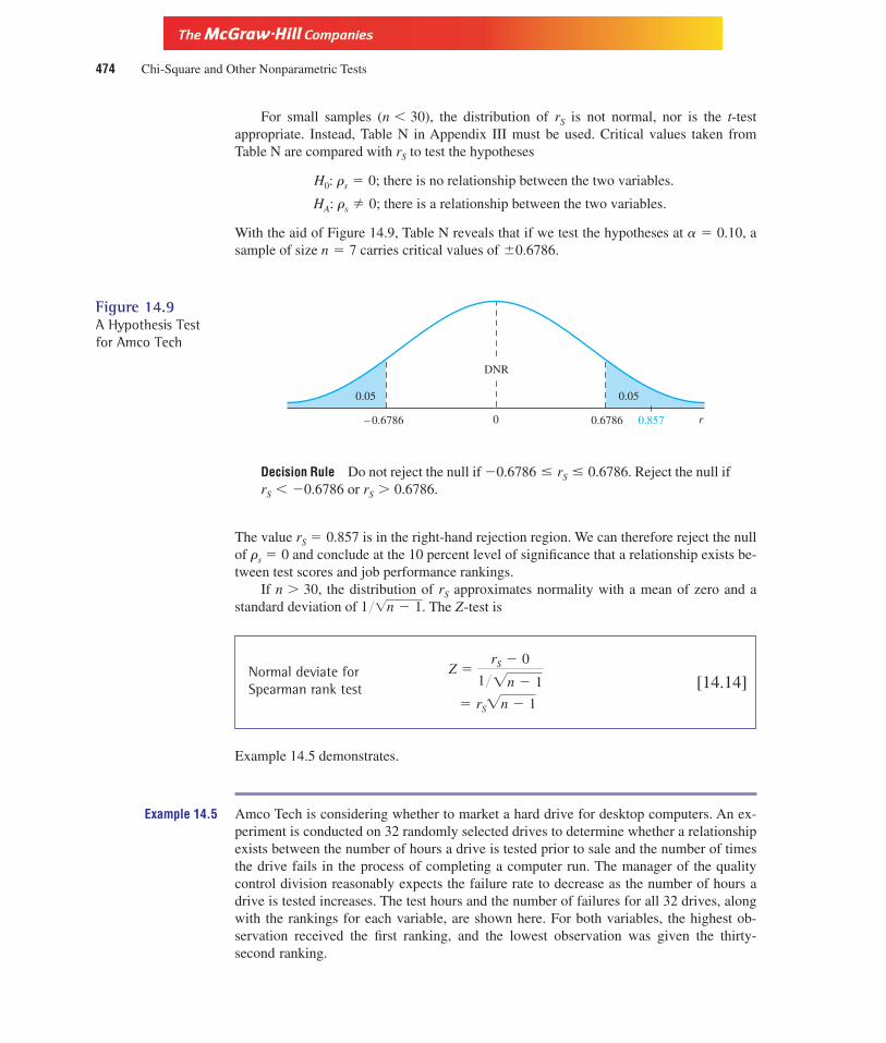
Version, Third Edition
For small samples (n � 30), the distribution of rS is not normal, nor is the t-testappropriate. Instead, Table N in Appendix III must be used. Critical values taken fromTable N are compared with rS to test the hypotheses
With the aid of Figure 14.9, Table N reveals that if we test the hypotheses at a � 0.10, asample of size n � 7 carries critical values of �0.6786.
HA: rs � 0; there is a relationship between the two variables.
H0: rs � 0; there is no relationship between the two variables.
474 Chi-Square and Other Nonparametric Tests
0 r– 0.6786
0.05 0.05
0.6786 0.857
DNR
Figure 14.9A Hypothesis Testfor Amco Tech
Decision Rule Do not reject the null if �0.6786 rS 0.6786. Reject the null ifrS � �0.6786 or rS 0.6786.
The value rS � 0.857 is in the right-hand rejection region. We can therefore reject the nullof rs � 0 and conclude at the 10 percent level of significance that a relationship exists be-tween test scores and job performance rankings.
If n 30, the distribution of rS approximates normality with a mean of zero and astandard deviation of The Z-test is
Normal deviate for[14.14]Spearman rank test
Example 14.5 demonstrates.
Example 14.5 Amco Tech is considering whether to market a hard drive for desktop computers. An ex-periment is conducted on 32 randomly selected drives to determine whether a relationshipexists between the number of hours a drive is tested prior to sale and the number of timesthe drive fails in the process of completing a computer run. The manager of the qualitycontrol division reasonably expects the failure rate to decrease as the number of hours adrive is tested increases. The test hours and the number of failures for all 32 drives, alongwith the rankings for each variable, are shown here. For both variables, the highest ob-servation received the first ranking, and the lowest observation was given the thirty-second ranking.
� rS�n � 1
Z �rS � 0
1��n � 1
1��n � 1.

Version, Third Edition
Hours FailuresDrive Hours Ranking (X ) Failures Ranking (Y ) X � Y (X � Y )2
1 100 1.0 2 32.0 �31.0 961.002 99 2.5 3 30.5 �28.0 784.003 99 2.5 3 30.5 �28.0 784.004 97 4.0 4 28.5 �24.5 600.255 96 5.5 4 28.5 �23.0 529.006 96 5.5 5 27.0 �21.5 462.257 95 7.0 8 21.5 �14.5 210.258 91 8.0 6 25.5 �17.5 306.259 89 9.0 7 23.5 �14.5 210.25
10 88 10.5 10 17.5 �7.0 49.0011 88 10.5 8 21.5 �11.0 121.0012 80 12.0 9 19.5 �7.5 56.2513 79 13.0 9 19.5 �6.5 42.2514 78 14.5 10 17.5 �3.0 9.0015 78 14.5 11 15.5 �1.0 1.0016 77 16.0 7 23.5 �7.5 56.2517 75 17.5 12 13.5 4.0 16.0018 75 17.5 13 12.0 5.5 30.2519 71 19.0 11 15.5 3.5 12.2520 70 20.5 14 11.0 9.5 90.2521 70 20.5 12 13.5 7.0 49.0022 68 22.5 6 25.5 �3.0 9.0023 68 22.5 16 7.5 15.0 225.0024 65 24.0 15 9.5 14.5 210.2525 64 25.0 15 9.5 15.5 240.2526 60 26.5 16 7.5 19.0 361.0027 60 26.5 18 3.5 23.0 529.0028 58 28.0 19 2.0 26.0 676.0029 56 29.0 17 5.5 23.5 552.2530 55 30.5 20 1.0 29.5 870.2531 55 30.5 18 3.5 27.0 729.0032 50 32.0 17 5.5 26.5 702.25
10,484.00
Solution:
Set a � 0.01. A test of the hypothesis regarding the population correlation coefficientfollows:
The critical Z-value is �2.58. Then
� �5.14
Z � (�0.922)�32 � 1
HA: rs � 0
H0: rs � 0
� �0.922
rS � 1 �6(10,484)
32(322 � 1)
Chapter Fourteen 475

Version, Third Edition
Interpretation: The rS-value of �0.922 indicates a strong negative relationship between hours and failures.The longer a drive is tested before it is used, the fewer failures it experiences in complet-ing the run.
To use Minitab, enter the data for each variable in separate columns. Rank each withMANIP > Rank. Then click on STAT > BASIC STATISTICS > CORRELATION.Minitab will report rS.
14. Economists at the Mid-West Research Institute are conducting a study to analyze the relation-ship between people’s incomes and their consumption levels. Eleven consumers report thefigures below in thousands of dollars. At the 5 percent level of significance, does theSpearman rank correlation coefficient suggest a relationship?
Income 97 58 69 47 58 38 91 67 68 47 48Consumption 55 63 54 37 45 38 71 52 53 37 37
15. At the 10 percent level, is there a relationship between study time in hours and grades on atest, according to these data?
Time 21 18 15 17 18 25 18 4 6 5Grade 67 58 59 54 58 80 14 15 19 21
16. The rankings of the rates of return on 50 stocks are compared to the rankings on their price-earnings ratio yielding At the 5 percent level, what can you conclude about arelationship between the two stock variables?
17. Eighty-five men and 85 women rate a product yielding At the 1 percentlevel of significance, is there any correlation between the ratings based on gender?
14.7 Kruskal-Wallis TestThe Mann-Whitney U test serves as the nonparametric counterpart to the t-test for two in-dependent samples; we use it to compare two populations. If we need to compare morethan two populations, the Kruskal-Wallis test then applies as a logical extension of theMann-Whitney test, and we use it to test hypotheses regarding the distribution of three or
�d2i � 10,010.25.
�d2i � 19,412.5.
476 Chi-Square and Other Nonparametric Tests
Section Exercises
0 Z– 2.58
0.005 0.005
2.58– 5.14
As shown in the figure, the null should be rejected.1
1

Version, Third Edition
more populations. In this capacity, the Kruskal-Wallis test functions as the nonparametriccounterpart to the completely randomized design used in ANOVA tests. While the ANOVAtests depend on the assumption that all populations under comparison are normally distrib-uted, the Kruskal-Wallis test places no such restriction on the comparison.
Kruskal-Wallis Test A test that compares three or more populations to determinewhether a difference exists in the distribution of the populations. It is the analogue tothe F-test used in ANOVA tests.
The null hypothesis states that no difference exists in the distribution of the k popula-tions under comparison. The hypotheses are thus
H0: All k populations have the same distribution.
HA: Not all k populations have the same distribution.
The test requires that the observations be ranked, just as in the Mann-Whitney test.To illustrate, assume that, as the new accounts manager for Pox Skin Ointment, you
must compare the time it takes for three customers to pay for shipments of No-Flaw FaceCream, a new product offered by Pox. You randomly select several purchases for eachcustomer, along with the number of days each took to settle its account. The results areshown in Table 14.10. Notice that number of observations in all samples do not have tobe equal.
Chapter Fourteen 477
Table 14.10Number of Days toPay Pox for Delivery
Customer
Purchase 1 2 3
1 28 26 372 19 20 283 13 11 264 28 14 355 29 22 316 22 217 21
Each observation must then be ranked from lowest to highest. As with the Mann-Whitney, ties are assigned a rank equal to the mean ranking for those observations. Therankings are then summed for all k � 3 samples. Table 14.11 contains the results. TheKruskal-Wallis statistic is
Kruskal-Wallis test [14.15]
where ni is the number of observations in the ith samplen is the total number of observations in all samplesRi is the sum of the ranks of the ith sample
K �12
n(n � 1) ��R2
i
ni� � 3(n � 1)
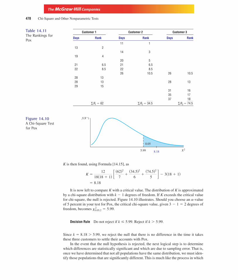
Version, Third Edition
K is then found, using Formula [14.15], as
It is now left to compare K with a critical value. The distribution of K is approximatedby a chi-square distribution with k � 1 degrees of freedom. If K exceeds the critical valuefor chi-square, the null is rejected. Figure 14.10 illustrates. Should you choose an a-valueof 5 percent in your test for Pox, the critical chi-square value, given 3 � 1 � 2 degrees offreedom, becomes
Decision Rule Do not reject if k 5.99. Reject if k 5.99.
Since k � 8.18 5.99, we reject the null that there is no difference in the time it takesthese three customers to settle their accounts with Pox.
In the event that the null hypothesis is rejected, the next logical step is to determinewhich differences are statistically significant and which are due to sampling error. That is,once we have determined that not all populations have the same distribution, we must iden-tify those populations that are significantly different. This is much like the process in which
x 20.05,2 � 5.99.
� 8.18
K �12
18(18 � 1) �(62)2
7�
(34.5)2
6�
(74.5)2
5 � � 3(18 � 1)
478 Chi-Square and Other Nonparametric Tests
Table 14.11The Rankings forPox
Customer 1 Customer 2 Customer 3
Days Rank Days Rank Days Rank
11 113 2
14 319 4
20 521 6.5 21 6.522 8.5 22 8.5
26 10.5 26 10.528 1328 13 28 1329 15
31 1635 1737 18
∑R1 � 62 ∑R2 � 34.5 ∑R3 � 74.5
5.99 8.18
0.05
X2
f (X2)Figure 14.10A Chi-Square Testfor Pox

Version, Third Edition
we used the Tukey methods to detect significant differences in our study of ANOVA. Aswith the Tukey approach, this involves a pair-wise comparison of all possible pairs.
We must first compute the average rank for each sample by dividing the sum of thesample’s rank by the number of observations in that sample. For the first sample this is
Similarly, and . The absolute differences are found as
These absolute values are then compared to a critical value to determine whether they dif-fer significantly. This critical value Ck is calculated as
Critical value for theKruskal-Wallis test [14.16]
where is the chi-square value used to test the original hypothesis, 5.99 inthis case
ni and nj are the sizes of the two samples under comparison
If the actual difference between the average ranks of the two samples is greater than thecritical difference, it is considered a significant difference and the two populations arefound to be different.
If we have a balanced design with equal size samples, Ck will be the same for all pair-wise comparisons. If the design is unbalanced as in this case, a different value for Ck mustbe computed for each comparison. To compare customer 1 and customer 2 for Pox, Ck is
Since is less than 7.27, populations 1 and 2 do notdiffer. In a similar manner, Ck for populations 1 and 3 is 7.65. Since the observed absolutedifference between 1 and 3 is 6.04 � 7.65, these two populations are not different. Finally,Ck for populations 2 and 3 is 7.91. The actual difference between 2 and 3 is 9.15 7.91,and populations 2 and 3 are said to be different.
Common underscoring can be used to summarize based on the average ranks.
R�2 R�1 R�3
5.75 8.86 14.9
Minitab Display 14.5 provides the results for the Pox test. The H � 8.18 is the k-valuewe calculated above. The p-value of 0.017 is also given.
}R1 � R2} � }8.86 � 5.75} � 3.11
� 7.27
Ck � �5.99� (18)(19)12 �� 1
7�
1
6 �
x 2a, k�1
Ck � �x 2a,k�1 �n(n � 1)
12 �� 1
ni
�1
nj�
}R2 � R3} � }5.75 � 14.9} � 9.15
}R1 � R3} � }8.86 � 14.9} � 6.04
}R1 � R2} � }8.86 � 5.75} � 3.11
R3 �74.5
5� 14.9R2 �
34.5
6� 5.75
R1 �62
7� 8.86
Ri
Chapter Fourteen 479

Version, Third Edition
Minitab Display 14.5Kruskal-Wallis Test
LEVEL NOBS MEDIAN AVE. RANK Z VALUE1 7 22.00 8.9 -0.412 6 20.50 5.7 -2.113 5 31.00 14.9 2.66
OVERALL 18 9.5
H = 8.18 d.f. = 2 P = 0.017H = 8.24 d.f. = 2 p = 0.017 (adjusted for ties)
It should be apparent by now that it is possible to substitute certain nonparametric testswhen essential assumptions required for those statistical procedures studied in earlier chap-ters may not hold. In the absence of specific conditions such as a normally distributed pop-ulation, these nonparametric tests may be the only appropriate course of action.
Table 14.12 compares nonparametric tests with their parametric counterparts. Whereappropriate, the parametric analogue for each nonparametric test is shown. The table alsoindicates the assumptions required by the parametric tests that are not necessary to conductthe nonparametric counterpart.
480 Chi-Square and Other Nonparametric Tests
Table 14.12A Comparison ofParametric andNonparametric Tests
Nonparametric Assumption Not ParametricTest Purpose Required Counterpart
Sign Test for location of Normal distribution t-test for matchedpopulation distribution of populations pairs
Runs Test for randomness None
Mann-Whitney Compare two Difference between t-test forU independent samples samples is normal independent samples
Kruskal-Wallis Compare three or Sample means normally F-test with ANOVAmore samples distributed
Spearman rank Test for relationship between Distribution of both Pearsonian correlationtwo ordinally ranked variables variables is normal coefficient
18. Recently, Bytec, Inc., has had a problem with employee absenteeism at its three productionplants. Based on the data below, taken over a six-day period for the number of employeeswho are absent, does it seem at the 5 percent level of significance that there is a difference inthe number of employees who fail to show for work? If you reject the null, perform a pair-wise comparison complete with common underscoring.
Number of Absent Employees
Plant 1 25, 36, 38, 31, 29, 33Plant 2 31, 28, 39, 41, 21, 20Plant 3 29, 28, 22, 26, 24, 20
19. To test a new pet food, Puppy Love feeds four groups of 10-week old puppies different mealmixes. After three weeks the increase in weights are recorded. Is there a significant differencein the weight increases at the 5 percent level? If you reject the null, perform a pair-wisecomparison complete with common underscoring.
Section Exercises

Version, Third Edition
Increase in Weights(pounds)
Mix 1 3, 6, 9, 5, 6Mix 2 3, 4, 8, 9, 7Mix 3 10, 8, 9, 8, 7Mix 4 8, 10, 11, 8, 8
20. Security Investments uses three methods to select stocks for their portfolio. At the 5 percentlevel, is there a difference in the rates of return for each method based on these data? If youreject the null, perform a pair-wise comparison complete with common underscoring.
Rates of Return(percentages)
Portfolio 1 14, 12, 10, 15, 13Portfolio 2 9, 6, 8, 5, 5Portfolio 3 6, 8, 5, 9, 7
Solved Problems1. 2B or not 2B—A Quality Control Problem According to U.S. News & World Report, a
laboratory in Atlanta is processing snake venom for use in medical research. Five processingmethods are being tested to determine which is least likely to contaminate the processedvenom. If a venom solution is tested as contaminated, it is marked with the symbol “2B.”Each method produces 25 vials of venom each day. The vials from each processing methodare then boxed for shipment to medical research facilities.
Assume for our purposes that scientists in the laboratory feel that the contamination isuniformly distributed, but others argue that it is binomially distributed. A statistical consultantis retained to examine defect patterns.
a. Is Contamination Uniform? Output over a 100-day period is selected for each process-ing method, and notation is made as to which method produced the fewer contaminatedvials that day. If contamination rates were uniform, the scientists would expect eachmethod to produce the fewest contaminated vials on an equal number of days. Thus,
Both observed and expected frequencies are shown in theaccompanying table. For example, on 34 of the 100 days, method 1 produced thefewest contaminated vials of snake venom. The hypotheses are
Processing Method Ei Oi (Oi � Ei)2 (Oi � Ei)
2/Ei
1 20 34 196 9.802 20 17 9 0.453 20 14 36 1.804 20 12 64 3.205 20 23 49 0.45
100 100 15.70
With K � 1 � 4 degrees of freedom, Table H (Appendix III) shows that a 1 percenttest reveals a critical x 2-value of As shown in the figure, the decisionrule is
x 20.01,4 � 13.277.
HA: Contamination rates are not uniform.
H0: Contamination rates are uniform.
� 100�5 � 20.Ei � n�k
Chapter Fourteen 481

Version, Third Edition
Decision Rule Do not reject if Reject if
Since 15.7 13.277, we reject the null. The contamination rates do not appear to beuniform.
� 15.7
x 2 � � (Oi � Ei)2
Ei
x 2 13.277.x 2 13.277.
482 Chi-Square and Other Nonparametric Tests
f (X2)
X215.7
0.01
13.277
b. Is Contamination Binomial? Those scientists in the laboratory who support the idea of abinomial contamination pattern argue that 5 percent of the vials produced are contami-nated. Given the 5 percent rate, the statistical consultant is to test the following hypo-theses:
The test is first applied to method 1. Each box contains n � 25 vials. If a binomial distribu-tion exists in contamination rates with as the scientists argued, the probabilitythat any box contains a given number of contaminated vials, X, is found in the binomialtable. For example, if n � 25 and , the probability that a box contains zero conta-minated vials can be found from Table C (Appendix III) as� 0.2744. The probability that only 1 of the 25 vials is contaminated can be found fromTable C as P(X 1) � P(X 0) � 0.6424 � 0.2740 � 0.3650, and so on. Thus, theexpected number of boxes out of the 100 samples that contain zero contaminated vials isnPi � (100)(0.2774) � 27.74 boxes. Notice that for purposes of determining the P(x)from the binomial table, n � 25 because there are 25 vials in each box. For determining thenumber of boxes with x contaminated vials, n � 100 because there are 100 boxes.
The values of Ei and Oi are shown in the tables below. The first table shows that 31 ofthe 100 boxes from method 1 had zero contaminated vials.
Number ofContaminated Vials Oi P(X ) Ei
0 31 0.2774 27.741 32 0.3650 36.502 24 0.2305 23.053 10 0.0930 9.304 2 0.0269 2.69
5 or more 1 0.0072 0.72100
However, some of the values for Ei are less than 5. The last three classes must be com-bined to correct for this. The second table is the result.
P(X � 0}n � 25, p � 0.05)p � 0.05
p � 0.05
HA: Contamination rates are not binomial.
H0: Contamination rates are binomial.
1

Version, Third Edition
Number ofContaminated Vials Oi P(X ) Ei (Oi � Ei)
2/Ei
0 31 0.2774 27.74 0.38311 32 0.3650 36.50 0.55482 24 0.2350 23.50 0.0106
3 or more 13 0.1226 12.26 0.0447100 0.9932
If
Decision Rule Do not reject if Reject if x 2 7.815.
Since x 2 � 0.9932, we do not reject the null. Contamination rates appear to be binomi-ally distributed.
2. The Sign Test—A Case of Quality Control In an effort to improve its product, a firm sell-ing bakery products asks 15 taste testers to rate its whole wheat bread between 0 and 10 be-fore and after a slight change in the ingredients. The results are partially shown in the table.
Tester Rating Before Rating After Sign
1 7 8 �
2 6 6 03 9 8 �
4 5 7 �. . . .. . . .. . . .
15 8 7 �
In total, eight plus signs, five minus signs, and two zero differences were recorded. Thefirm wants to test at the 5 percent level whether there is any difference. Thus,
Then
The probability of getting at most five minus signs given m � p is greater than 0.05�2 �0.025. The firm does not reject the null.
If the sample size had exceeded 30, the Z-test Formula [14.4] would have been used.
3. A Mann-Whitney U Test of Means Two advertising displays are used to aid the sales of aproduct. The first display resulted in daily sales of 110, 117, 82, 95, 123, 79, 92, 102, 108, and113. The second display produced sales of 111, 85, 97, 117, 111, 89, 118, 121, and 109.Would it appear that at the 5 percent level, m1 � m2?
Display 1 Rank Display 2 Rank
79 1 85 382 2 89 492 5 97 795 6 109 10
102 8 111 12.5108 9 111 12.5110 11 117 15.5113 14 118 17117 15.5 121 18123 19
90.5 � R1 99.5 � R2��
P(m 5}n � 13, p � 0.50) � 0.2905
HA: m � p
H0: m � p
x 2 7.815.
a � 0.05, x 20.05,3 � 7.815.
Chapter Fourteen 483

Version, Third Edition
If a is set at 5 percent, the critical Z-value is �1.96.
484 Chi-Square and Other Nonparametric Tests
0 Z–1.96
0.025 0.025
1.960.7757
The sample suggests that the null is not to be rejected, and that both displays have the sameeffect on sales.
4. Spearman Rank Correlation A financial consultant is asked to evaluate the investmentqualities of eight stocks. She uses the stock’s dividend rate as reported in The Wall StreetJournal and an index potential for growth assigned to each stock by a New York investmentfirm. The data are shown here and are used to determine whether a relationship might existbetween dividends and growth potential.
� 0.7757
�54.5 � 45
12.247
Z �Ui � mu
su
� 12.247
su � �n1n2(n1 � n2 � 1)12
� 45
mu �n1n2
2
� 35.5
� (10)(9) �9(9 � 1)
2� 99.5
�n2(n2 � 1)
2� �R2U2 � n1n2
� 54.5
� (10)(9) �10(10 � 1)
2� 90.5
�n1(n1 � 1)
2� �R1U1 � n1n2
HA: m1 � m2
H0: m1 � m2
1

Version, Third Edition
Dividend Dividend GrowthStock Rate (%) Ranking (X ) Index Growth Ranking (Y ) X � Y (X � Y )2
1 4.20 7 40 6 1 12 8.12 2 20 8 �6 363 7.20 5 60 4 1 14 3.20 8 35 7 1 15 8.00 3 85 1 2 46 12.73 1 70 2 �1 17 7.90 4 50 5 �1 18 6.20 6 65 3 3 9
54
If a � 0.10, test
Table N (Appendix III) reveals a critical value of 0.6190. Therefore, do not reject the null.
List of Formulas
[14.1]The chi-square is used to compareobserved frequencies with those frequen-cies we would expect if the null is correct.
[14.2] The expected frequencies are those wewould expect to happen if the null is cor-rect.
[14.4] Z-value for a large-sample sign test.
[14.5]Mean of the sampling distribution of thenumber of runs.
[14.6] Standard deviation for the runs test.
[14.7] Normal deviate for the distribution of runs.
[14.8]The Mann-Whitney U statistic tests theequality of two populations.
[14.10]Mean of the sampling distribution of theMann-Whitney U statistic.
[14.11]Standard deviation of the Mann-WhitneyU statistic.
[14.12]Normalization of the Mann-Whitney U statistic.Z �
Ui � mu
su
su � �n1n2(n1 � n2 � 1)12
mu �n1n2
2
U1 � n1n2 �n1(n1 � 1)
2� �R1
Z �r � mr
sr
sr � � 2n1n2(2n1n2 � n1 � n2)(n1 � n2)
2(n1 � n2 � 1)
mr �2n1n2
n1 � n2
� 1
Ztest �k � 0.5 � 0.5n
0.5�n
Ei � npi
x 2 � �K
i�1
(Oi � Ei)2
Ei
HA: PS � 0H0: PS � 0
� 0.357
� 1 �6(54)
8(82 � 1)
rS � 1 �6�d 2
i
n(n2 � 1)
Chapter Fourteen 485

Version, Third Edition
[14.13]The Spearman rank correlation coefficienttests for any relationship between ordi-nally ranked variables.
[14.14] Normal deviate for the Spearman rank testwith large samples.
[14.15]The Kruskal-Wallis test is used tocompare three or more populations.
[14.16]Determines the critical value in a Kruskal-Wallis Test for pair-wise comparisons.
Chapter Exercises21. You have been asked by your supervisor to determine whether there is a relationship between
the type of capital budgeting technique a firm uses and its net income after taxes. The datayou collect relate three techniques—net present value, internal rate of return, and profitabilityindex—to four income levels: 0 to $3 million, $3 million to $6 million, $6 million to $9 mil-lion, and above $9 million. The number of firms falling in the joint categories has been tabu-lated. What statistical tool would you use to detect any relationship?
22. You are to compare the mean spending levels of three groups of consumers, but you cannotassume that the populations are normally distributed or that their variances are equal. Whattool should you use?
23. As regional manager for a retail firm, you want to determine whether people’s income levelsand their consumption patterns are related. What tool should you use?
24. An economist for an international bank holding company collected data on the consumptionlevels of 25 people before and after the federal government announced a large tax increase.What tool will allow the economist to determine whether the tax affected mean consumption?
25. You are to select a sample of your firm’s customers based on gender. How can you determinewhether the sampling procedure is random?
26. Your statistical assistant has obtained data on two independent samples taken to comparepeople’s ages. If it cannot be assumed that the populations are normal, what test should he use?
27. Why do we use nonparametric tests? Why not always rely on parametric tests, since they arestronger?
28. What is being measured by a sign test?
29. What is measured by a runs test?
30. Cite your own example in which the Spearman test would be required, and describe exactlywhat it is you are measuring in this example.
31. A bank in Des Moines wants to determine whether the distribution of customers is uniformthroughout the week. A survey finds that the numbers of customers Monday through Fridayare 150, 179, 209, 79, and 252. At the 5 percent level, does it appear that a uniform distribu-tion exists?
a. State the hypotheses.b. State the decision rule.c. Conduct the test and make your determination.
32. Professor Showers argues that his grade distribution is 5 percent A’s, 20 percent B’s, 30 percentC’s, 40 percent D’s, and the rest F’s. If this is the case, his dean has promised him a 15 percent
Ck � �x2a,k�1
n(n � 1)12 � 1
ni
�1
nj�
K �12
n(n � 1) ��R2
i
ni� � 3(n � 1)
Z � rs�n � 1
rS � 1 �6�d 2
i
n(n2 � 1)
486 Chi-Square and Other Nonparametric Tests

Version, Third Edition
raise. At the 1 percent level, does the kind professor get his raise if 100 randomly selectedgrades provide this breakdown: 7 A’s, 20 B’s, 27 C’s, 36 D’s, and 10 F’s?
33. Creative Floorings has decided to order its supplies in bulk if the size of carpet placed inhomes is normally distributed. Help the company managers make this decision based on thefollowing sample data. Set alpha at 1 percent.
Square Yards Number of Houses(100’s) of This Size
Up to 5 975 to 10 137
10 to 15 24515 to 20 25620 to 25 15425 and above 111
34. The frequency table shown records daily sales for 200 days. At a � 0.05, do sales appear tobe normally distributed?
Sales Frequency
40 up to 60 760 up to 80 2280 up to 100 46
100 up to 120 42120 up to 140 42140 up to 160 18160 up to 180 11180 up to 200 12
35. Citizens for a Nonviolent Media provided data that were subsequently published in a recentissue of U.S. News & World Report on the number of acts of violence seen in types to televi-sion programs. The organization claimed that such acts occur with equal frequency across allprogram types. Test this claim at the 10 percent level.
Type of Program Acts of Violence
Drama 42Old movies 57Cartoons 83Police/detective 92Comedy 38News 81
36. Greenpeace, the worldwide conservation group, recently called for a United Nations sanctionon the killing of baby harp seals in what it called “high mortality months.” Finland, which stillpermits these “harvests,” stated that the activity was consistent throughout the year and didnot vary by month. Given the data for 1997 provided by Greenpeace, what conclusion canyou reach? Set alpha at 1 percent.
Month Number of Kills
January 112February 89March 156April 104May 165
Chapter Fourteen 487

Version, Third Edition
37. The production manager of AAA, Inc., must ensure that his product mix fits a particular quotasystem. He is instructed to adjust to a pattern that produces 30 percent silk goods, 20 percentwool, 10 percent cotton, and 40 percent leather. Of the last 200 units produced, 65 were silk,45 were wool, 25 were cotton, and 65 were leather. At the 5 percent level, should he adjust thecurrent production pattern? State the hypotheses.
38. A retail chain has six outlets. It has been spending heavily to produce similar sales levels at allsix stores. The advertising firm handling the promotional efforts claims that now each storeshould report equal sales. If sales are not the same, the retail chain has decided to discontinueits association with the ad agency. What decision should be made based on the data shownhere? State your hypotheses. Set a � 0.01.
Store Sales ($100’s)
1 422 373 534 515 456 47
39. Macy’s department store in New York recently did a study to determine whether there wasany relationship between a customer’s marital status and his or her dollar volume of pur-chases. The results are shown in the table. What is your conclusion at the 5 percent level ofsignificance?
Dollar Volume
,10 10–19 20–29 30–39 40–49
Married 32 23 15 12 14Divorced 51 17 10 15 13Single 21 19 29 35 39Widowed 18 15 19 10 9
40. The U.S. Treasury Department has estimated that the “increase in the typical taxpayer’s feenecessary to balance the budget is uniformly distributed across states.” The February 28,1994, issue of U.S. News & World Report published the following statistics:
Average Taxpayer’s HikeState (Top 10 States)
Connecticut $1,100New Jersey 952New York 877Massachusetts 852DC 851Maryland 840Nevada 828Illinois 822Washington 809California 789
At the 5 percent level, can the Treasury Department be supported?
41. The General Store will determine sales dates based on the distribution of revenues. Given thedata below, does it appear at the 5 percent level that revenues are normal? The mean is knownto be 25.6, and s is 10.1.
488 Chi-Square and Other Nonparametric Tests

Version, Third Edition
Revenue/Month ($100’s) Number of Months
Up to 10 1010 to 20 2320 to 30 3030 to 40 2540 and above 12
42. Consider the data below for job completion times, which were taken from a population with amean of 18 and a standard deviation of 4.
Times (Hours) Number of Jobs
Up to 10 1010 to 15 10115 to 20 22320 to 25 14625 and above 20
a. At the 5 percent level, can it be concluded that times are normally distributed?b. How do the results differ if the first inteval is “5 to 10” and the last is “25 to 30”?
43. The chief economist at the state revenue office is debating with his supervisor who argues thattax payments are normally distributed. Data on 2,000 taxpayers provided the results seen here.At the 1 percent level, is the supervisor correct?
Tax Payment ($10’s) Taxpayers
Up to 15 24815 to 30 23230 to 45 48945 to 60 51260 to 75 26375 and above 256
44. Runner’s World reported that a survey by Converse of people who regularly run for exercise re-sulted in the data shown here. The intent of the survey was to determine whether the distanceswere independent of runners’preference for a gel-like product built into the heels of their jog-ging shoes. At the 1 percent level, does there appear to be any relationship? State the hypotheses.
Distance/Week(miles) Prefer Gel Do Not Prefer Gel No Opinion
�3 14 5 273–6 18 5 177–10 12 8 8
10–13 17 12 513 19 8 2
45. Data on years of experience and efficiency ratings for 431 employees at XYZ, Inc. are shown inthe table. Can you conclude that these attributes are independent of each other? Set a � 5 percent.
Efficiency
Experience in Years Poor Good Excellent Superior
�5 14 18 12 175–10 18 13 27 42
11–16 16 32 24 3717–22 24 28 21 3222 17 15 14 10
Chapter Fourteen 489

Version, Third Edition
46. The results of a study by the American Marketing Association to determine the relationshipbetween the importance store owners attach to advertising and the size of store they own areshown in the table. Would it seem that all store owners place the same emphasis on advertis-ing? Set a � 0.10. State the hypotheses.
Advertising
Size Important Not Important No Opinion
Small 20 52 32Medium 53 47 28Large 67 32 25
47. A bottling company in Atlanta is interested in the effects of three methods used to sanitize glasscontainers. It grades containers to determine whether sanitation is independent of the method.At the 10 percent level of significance, what is your conclusion based on the data in the table?
Sanitation Grade
Method Acceptable Marginal Unacceptable
A 140 132 63B 89 74 44C 104 98 50
48. Eight test subjects are asked to rate a product before and after viewing a commercial for it. Theratings are shown in the table, where a rating of 10 is best. Set a � 0.10 and use a sign test forthe hypothesis that the commercial improved the product’s rating. State the hypotheses.
Ratings
Test Subject Before Commercial After Commercial
1 8 92 7 63 5 64 5 55 5 46 7 87 6 78 6 8
49. A chemical compound is added to an oil base solution in hopes of increasing its lubricatingqualities. Twenty solutions, 10 with the compound and 10 without, are compared with respectto their ability to lubricate machinery. Each is graded on a scale from 0 to 10, with 10 beingthe best. Based on the data in the table, does it appear that addition of the compound increaseslubrication? Set a � 0.10. State the hypotheses. What is your conclusion regarding the valueof the chemical compound?
Lubrication Grade
Solution Without Compound With Compound
1 8 42 7 83 5 24 6 95 9 56 4 47 9 28 8 69 7 6
10 6 7
490 Chi-Square and Other Nonparametric Tests

Version, Third Edition
50. Shytel, Inc. offers communication services anywhere in the world with two satellites, theFalcon and the Eagle. Shytel’s CEO thinks that the Eagle results in longer delays in transmis-sion. Transmission times are shown in minutes in the table. At the 5 percent level, does it ap-pear that the CEO is correct? State your hypotheses.
Transmission Times (minutes)
Falcon Eagle Sign
5.2 4.7 �
8.6 7.9 �
9.0 9.7 �
4.3 8.4 �
6.2 3.7 �
7.9 7.3 �
51. Clyde Bloomquist has proposed a change in corporate policy concerning collection ofaccounts receivable. He feels it will speed the time required to obtain outstanding debts fromcreditors. Company records show that eight creditors took the number of days shown in thetable before and after the policy change to remit funds due. Is Clyde correct? Should the pol-icy change be retained? Set a � 0.10. State the hypotheses.
Creditor Before After
1 18 122 27 223 32 314 23 245 31 286 36 247 18 168 35 25
52. Shoppers in a large mall in Dayton were randomly asked which of two brands of yogurt theypreferred. Forty-two said Swedish Heaven, 31 chose Merry Melody, and 12 expressed nopreference. If the local yogurt shop is to carry only one brand, which should it be? Seta � 0.10. State the hypotheses.
53. A manufacturer uses parts from either supplier A or supplier B to make his product. A checkof yesterday’s output reveals that the order in which these suppliers’ parts were used was
AA BBB AAA B A BB AA BB
Does it appear that the parts are being used randomly? Set a � 0.05. State your hypothesesand conclusion.
54. Smile Bright sells toothpaste in 17-ounce containers. Management expects overfills and under-fills to be random. If they are not, management assumes something is wrong with the fill system,and shuts down the production line. Should the line be shut down if containers measure 16.8,18.2, 17.3, 17.5, 16.3, 17.4, 16.1, 16.9, 17, 18.1, 17.3, 16.2, 17.3, and 16.8 ounces? Let a � 0.05
55. Sales receipts are recorded for the past 37 days. You denote those values below the medianwith a “B” and those above it with an “A.” Counting the results, you find 18 A’s and 19 B’swith 10 runs. Your policy is to increase advertising if receipts are not randomly distributed.Should you increase advertising? State the hypotheses. Let a � 0.05.
56. Acme Plumbing bids on construction jobs for city buildings. If contracts are granted by thecity without regard to political consideration, Acme should witness no pattern in whether itsbid is accepted or rejected. For the last 63 bids, Acme has had 32 accepted and the rest re-jected, with 27 runs. At the 5 percent level, would it appear that bids are let on the basis ofpolitics? State the hypotheses, the decision rule, and your conclusion.
Chapter Fourteen 491

Version, Third Edition
57. Gladys Glucose offers vanilla- and chocolate-flavored ice cream to visitors in the park. Thelast 73 sales consisted of 40 vanilla and 33 chocolate, with 16 runs. If sales are not random,Gladys will move her ice cream truck to the local zoo. Where should she set up business? Leta � 0.05.
58. A large company hired 52 men and 41 women, resulting in 32 runs. If absence of randomnessin the hiring process indicates discrimination, can it be alleged that the company practices sexdiscrimination in its hiring practices? Set a � 0.10.
59. Over a 12-day period, Gladys Glucose sold 4, 11, 5, 7, 10, 13, 12, 5, 9, 6, 2, and 1 gallons ofvanilla, and 19, 4, 6, 8, 18, 17, 17, 15, 3, 16, 14, and 0 gallons of chocolate. Using the Mann-Whitney U test, can she conclude that she sells the same amount of both flavors on the aver-age? Set a � 0.01.
60. The marketing director for Software, Inc., treated 15 computer disks with a solution designedto reduce wear. A second solution was used to treat 15 other disks, and all were graded on thebasis of wear. Those treated with the first solution showed improved wear, measured in hoursof use of 65, 73, 82, 52, 47, 51, 85, 92, 69, 77, 84, 68, 75, 74, and 89 hours. Those subjectedto the second solution reported increased wear times of 73, 84, 91, 87, 90, 71, 72, 93, 99, 98,89, 88, 79, 88, and 98 hours. At the 10 percent level, can the director conclude that there isany difference in the improved wear factors?
61. The quality control manager for a large plant in Denver gives two operations manuals to twogroups of employees. Each group is then tested on operations procedures. The scores areshown in the table. The manager has always felt that manual 1 provides a better base ofknowledge for new employees. Compare the mean test scores of the employees shown hereand report your conclusion. State the hypotheses. Set a � 0.05.
Employee Test Scores
Manual 1 87 97 82 97 92 90 81 89 90 88 87 89 93Manual 2 92 79 80 73 84 93 86 88 91 82 81 84 72 74
62. Two manufacturing processes are used to make I-beams for construction of large buildings.Each I-beam is tested, and its tensile strength is recorded. Twenty-three beams made with thefirst process result in and 27 beams made via the second process produce
A construction engineer argues that the first process results in beams that have atleast the tensile strength demonstrated by beams made by the second process. At the 5 percentlevel, is she right?
63. An agricultural economist treats 50 acres of land with the chemical docide to increase cropyield. Fifty other acres are treated with mildolmine, and yields are measured. and
The economist tells farmers that docide, which is a cheaper chemical, will pro-duce a yield higher than mildolmine. At the 10 percent level, is he correct? State the hypotheses.
64. Personnel Management carried an article describing efforts by a manufacturing firm in Toledoto evaluate its supervisors. Employees were asked to rate their supervisors on a scale of 10 to100. A subset of the results is shown here for three of the work areas. Determine whether adifference exists in the ratings received by the supervisors. State the hypotheses, the decisionrule, and your conclusion. Set a at 5 percent.
Shop Office Loading Dock
40 63 5052 59 5263 55 6381 61 5572 48 7172 53 45
49
�RM � 2,925.�RD � 2,125
�R2 � 585.�R1 � 690,
492 Chi-Square and Other Nonparametric Tests

Version, Third Edition
65. A total of 48 service calls are sampled by a local plumbing contractor to determine which offour types of plumbing fixtures produce the most problems. The results are shown here.
Fixture Model Number of Failures
1 152 113 104 12
At the 1 percent level of significance, does the failure of the fixtures appear to be uniformlydistributed? State your hypotheses, decision rule, and conclusion.
66. Four methods of treating steel rods are analyzed to determine whether there is any differencein analyzed the pressure the rods can bear before breaking. The results of tests measuring thepressure in pounds before the rods bent are shown. Conduct the test, complete with the hy-potheses, decision rule, and conclusion. Set a � 1 percent.
Method 1 Method 2 Method 3 Method 4
50 10 72 5462 12 63 5973 10 73 6448 14 82 8263 10 79 79
67. The World’s-Second-Best-Yogurt asks 60 people which of four new yogurt flavors they pre-ferred. Twenty-one chose coconut-pickle, 13 chose prune with ketchup topping, 10 selectedmustard á la peanut butter, and 16 expressed a partiality for essence of tuna. Does there appearto be a preference among the flavors by the customers? Set a at 10 percent. State the hypo-theses and your conclusion.
68. For extra credit in her statistics course, Barbara must determine whether there is a differencein the average number of hours spent studying by freshmen, sophomores, juniors, and seniorsat her university. Her research revealed the following:
Freshmen Sophomores Juniors Seniors
20 18 22 2929 9 19 3110 12 21 2717 15 31 2215 14 42 1823 22 22 3127
Help Barbara earn her extra credit in statistics by stating her hypotheses and conclusion. Seta � 10 percent.
69. As product manager of Sports Wear, Inc., Beverlee Hills must ensure that the sizes of itsnew line of active wear are produced according to a certain predetermined pattern. The mar-ket research indicates that customers prefer 20 percent extra large, 30 percent large, 25 per-cent medium, and 25 percent small. A random sample of 145 garments reveals 32 extralarge, 40 large, 41 medium, and 32 small. At the 5 percent level, does it appear that thedesired proportion of sizes is being observed?
70. Ms. Hills, from the previous exercise, must determine whether the spending habits of variousdemographic groups are the same. She examines the size of typical purchases, measured indollars, of four groups: married males (MM), married females (MF), single males (SM), andsingle females (SF). She finds the following information.
Chapter Fourteen 493

Version, Third Edition
MM MF SM SF
$50 $20 $19 $8717 23 32 2023 82 66 9548 46 72 3463 13 41 11
At the 1 percent level of significance, does it appear that a difference exists in spending habitsof these four groups?
71. Seven corporate bond issues are ranked as to their investment worth by two financial analysts.The results are shown here. Using these rankings as a sample, calculate the Spearman rankcorrelation test to determine whether there is any correlation between the rating practices ofthese two analysts at the 10 percent level.
Rating of Rating ofCorporation First Analyst Second Analyst
1 4 32 3 43 1 24 2 55 7 66 6 17 5 7
72. Six truck models are rated on a scale of 1 to 10 by two companies that purchase entire fleets oftrucks for industrial use. Calculate the Spearman rank coefficient to determine at the 1 percentlevel whether the rankings are independent.
Rating by Rating byModel First Company Second Company
1 8 92 7 63 5 84 7 55 3 76 2 8
73. All 50 states are ranked by two travel agencies as to their desirability as a vacation spots. Theresults reveal Test for independence in ratings at the 10 percent level.
74. The top 10 firms on Fortune’s 500 list were ranked by the AFL-CIO and by a managementgroup on the basis of the quality of the health care system each company provides its employ-ees. Using the results shown here, determine at the 5 percent level whether there is any corre-lation in the rating practices of unions and management.
Union Management Union Management Firm Ranking Ranking Firm Ranking Ranking
1 5 6 6 6 42 8 10 7 1 83 2 3 8 9 14 7 9 9 3 25 4 7 10 10 5
75. Seventy-three employees are ranked by two managers on the basis of their productivity levels.Calculate the Spearman rank coefficient to determine whether the rankings are independent atthe 1 percent level of �d 2 � 78,815.
�d 2 � 22,712.
494 Chi-Square and Other Nonparametric Tests

Version, Third Edition
Chapter Fourteen 495
C U R T A I N C A L LIn order to help Mama resolve her prob-lems with Dante’s, as described in Set-ting the Stage, you must first determine
students’ preferences for pizza toppings. Surveying 135students, you find that 47 prefer pepperoni, 63 sausage, and21 cheese, whereas 4 want veggie pizza. Mama feels thesepreferences are uniformly distributed, while you think theyare more likely to fit a pattern described as 35 percent,45 percent, 15 percent, and 5 percent, respectively.
You try to fit a normal distribution to students’ ex-penditures based on your survey, which yielded the pat-tern described in the following frequency table. What areyour findings?
Expenditure Frequency
$0 and under $5 4$5 and under $10 11
$10 and under $15 45$15 and under $20 47$20 and under $25 25$25 and above 3
You also want to determine whether there is any re-lationship between the students’ preferences for large (L),medium (M), and small (S) pizzas and their status as
either graduate students (G) or undergraduates students(U). Your data show the following outcome:
L M S
U 51 19 9G 22 15 19
Mama is interested in whether there is a difference inthe mean number of times per week undergraduates eatout as compared to graduate students. Taking a subset of10 graduates and 10 undergraduates from your sample of135 students, you find these numbers to be
Student 1 2 3 4 5 6 7 8 9 10
Undergraduate 6 9 11 8 6 12 15 5 7 9Graduate 3 0 8 4 2 2 5 4 1 0
What do you report to Mama?Finally, you are to determine whether there is any re-
lationship for undergraduates between the number oftimes per week a student eats at Mama’s and his or her in-come. The ten undergraduates report incomes per week of$50, $60, $80, $55, $45, $90, $100, $50, $55, and $60respectively.
Prepare your report to Mama in the form of a statis-tical report, as described in Appendix I.
From the Stage to Real LifeAs the market analyst in the Setting the Stage chapter opener, you will likely want to gathermenu information from franchise companies such as Pizza Hut and Dominos. Their offer-ings in your own area or in similar college towns in other parts of the county can providenew ideas for you to test as well as to gain collaboration the results of your survey.
You can check out Pizza Hut menus at (http://www.pizzahut.com.hk). At the homepage, click on the animated pizza box. Then click on “Full Menu.” Here you can link to dif-ferent areas to see the variety of their pizza offerings as well as their pasta and appetizerand beverage menus. Explore these areas. Do you see any pizza combination specials ofpotential interest in your local market? Have you already included those in the survey youare doing for Mama’s Pizzeria? Are some of the appetizers appealing in your local marketas well as reasonable for offering within Mama’s operation? How might an extended menuhelp the business?
You can check out Domino’s offerings at (http://www.dominos.com). At the homepage, click on “Explore.” At the next page, click on “Pizza Fest.” Scroll down to the “To10!” link and click on it. After viewing this information, scroll to the bottom of the pageand click on “Pizza Oven.” The left column provides more extensive menu informationthan the Top 10! location. Answer the same questions that were posed for Pizza Hut.
Which of these sites is more helpful to you and why?

Version, Third Edition
496
C H A P T E R15Quality ControlTechniques

Version, Third Edition
497
Quality Control Techniques
R-chart
Associated risks
Role of theacceptance number
Sampling plans
Acceptance sampling
For variables
Control charts
X-chart–
c-charts
For attributes
p-charts
Chapter BlueprintAs competition for consumer dollars intensifies worldwide, the importance that a firm attaches to im-proving the quality of its product grows proportionately. This chapter explores the tests that a firmmay conduct to implement a quality control program designed to promote reliability and expand itscompetitive position in the market.

Version, Third Edition
S E T T I N G T H E S T A G E
498 Quality Control Techniques
Last year Minot Indus-tries, a major manufac-turer of glassware, was
forced to modernize its plant in Toledo tostay current with the level of technologymany of its competitors had adopted earlier.Since the plant was redesigned, Minot hasexperienced numerous problems with costoverruns, defective production, employeemorale, and other troublesome develop-ments.
Recently, Ray Murdock was appointedas the new chief executive officer (CEO) bythe major stockholders in Minot. The focusof Murdock’s rejuvenation efforts is to bringall production processes into compliancewith the quality standards for which Minotwas once revered in the industry.
Mr. Murdock realizes this will requirean extraordinary team effort on the part of
all his executive officers, as well as the linepersonnel who in the past have been faith-fully committed to the goals and aspirationsof Minot Industries.
In the past, Minot was able to main-tain its production standards with little ef-fort and with little concern for quality. Theraw materials used by its capable laborforce ensured that Minot would produce asuperior product. However, with increasedcompetition from both domestic and for-eign sources, maintaining product stan-dards at a reasonable cost has proved to bea more elusive goal.
Reestablishing Minot as an industryleader can be accomplished only throughthe application of precise methods of qualitycontrol. This is the challenge facing thoseloyal employees, who are willing to carryout their professional duties.
10
11
1 2 3 54
7
8
9
5
6
4
Sample Number
Sam
ple
Mea
n
LCL = 4.475
UCL = 9.665
X-Chart for Minot–
X = 7.070=
10
1 2 3 54
5
0
Sample Number
Sam
ple
Ran
ge
LCL = 0.4679
UCL = 11.91
R-Chart for Minot
R = 6.189–

Version, Third Edition
15.1 IntroductionOver the past several years the level of domestic and foreign competition has intensifiedconsiderably. This increased level of rivalry among business firms has created an ever-pressing need to monitor and maintain the quality of products. As competition stiffens, itbecomes increasingly difficult to acquire and retain a share of the market sufficient to per-mit economic survival. Without careful measures to ensure that its product meets certainminimum specifications, a business is even less likely to survive the harsh competitive con-ditions of today’s marketplace.
This chapter examines the numerous statistical tools that firms can use to administeran effective program to regulate the overall quality of their products, thereby making themmore competitive. A quality control program of this nature usually relies quite heavily ontechniques such as:
● Control charts for variables:-charts.
R-charts.
● Control charts for attributes:p-charts.c-charts.
● Operating characteristic curves.
● Acceptance sampling.
15.2 A Brief History of the World Development of Quality Control
Prior to the Industrial Revolution, production was carried out primarily by skilled artisans.So strong was the pride they took in their work that they often signed each finished piece.With the advent of the Industrial Revolution and the growth of the factory system, produc-tion became fragmented, with sole culpability for the product resting on no one in particu-lar. All too often, this shift in production methods minimized the worker’s identificationwith the product, and the care he or she took in completing a job. Production quality andcare for consumer needs dwindled as a result.
In the mid-1920s, Walter Shewhart, a researcher at Bell Laboratories, made an earlyand significant breakthrough in the area of product improvement. He recognized that, al-though variation in manufactured products was inevitable, this variation could be monitoredand controlled using certain statistical processes. He developed a simple graphical tool,called a control chart, to determine when this variation exceeded acceptable limits.
During World War II, the nation’s need for large quantities of high-quality war materi-als spurred further interest in control charts and related statistical tools, and promoted ageneral concern for quality control. However, it was not until the late 1970s, when U.S.manufacturers faced relentless competition from a flood of superior Japanese imports, thatU.S. interest in quality control became widespread.
W. Edwards Deming studied with Shewhart, and then took a position with the Depart-ment of Agriculture and later with the Census Bureau. Although he is now recognizedworldwide as one of the leading pioneers in the field of quality control, early on, only theJapanese studied his ideas seriously. Deming developed an entire philosophy of qualitymanagement based on his “14 points,” which state, among other things, that with theproper organizational climate, statistical methods of process improvement can reduce the
X
Chapter Fifteen 499

Version, Third Edition
variation referred to by Shewhart, decrease cost dramatically, and improve an organization’simage as well as its financial position. Deming argued that quality development was an on-going and never-ending process that required close and continual monitoring of the pro-duction process.
In 1951, Deming was invited to speak before the Japanese Union of Scientists andEngineers. The Japanese were concerned about the reputation they had developed for pro-ducing and exporting inferior, cheaply made products. In a lengthy series of lectures andmeetings with Japanese leaders in both industry and government, Deming convinced theJapanese that, by listening to the consumer and by applying statistical methods of qualitycontrol, they could expand their production and export products of high quality throughoutthe world. Deming’s ideas and teachings were instrumental in placing the Japanese in theenviable position they now enjoy as a world economic power. In his honor, the Japaneseestablished the Deming prize, which is given to companies recognized for outstandingquality improvement.
500 Quality Control Techniques
Table 15.1The MalcolmBaldrige NationalQuality AwardCriteria
Examination Categories/Items Point Values
1 Leadership 1101.1 Leadership System 801.2 Company Responsibility and Citizenship 30
2 Strategic Planning 802.1 Strategy Development Process 402.2 Company Strategy 40
3 Customer and Market Focus 803.1 Customer and Market Knowledge 403.2 Customer Satisfaction and Relationship
Enhancement 40
4 Information and Analysis 804.1 Selection and Use of Information and Data 254.2 Selection and Use of Comparative Information
and Data 154.3 Analysis and Review of Company Performance 40
5 Human Resource Development and Management 1005.1 Work Systems 405.2 Employee Education, Training, and Development 305.3 Employee Well-Being and Satisfaction 30
6 Process Management 1006.1 Management of Product and Service Processes 606.2 Management of Support Processes 206.3 Management of Supplier and Partnering
Processes 20
7 Business Results 4507.1 Customer Satisfaction Results 1307.2 Financial and Market Results 1307.3 Human Resource Results 357.4 Supplier and Partner Results 257.5 Company Specific Results 130
TOTAL POINTS 1,000
Source: 1997 Award Criteria, The Malcolm Baldrige National Quality Award, United StatesDepartment of Commerce.

Version, Third Edition
Joseph Juran was noted for preaching the benefits of quality control to the Japanese.As did Deming, Juran argued that a commitment by top management to quality controlwas essential. He stated that quality was the responsibility of managers, and that theyshould attend to it as they would to any other functional area such as finance or marketing.
Many awards have been developed to recognize achievement in American industry.Perhaps most notable is the Malcolm Baldrige National Quality Award. Established in1988 and named after the U.S. Secretary of Commerce from 1981 until his death in 1987,this award is designed to recognize those firms that exhibit a commitment to product ex-cellence. Past winners include Motorola (1988): Xerox (1989); and IBM, Federal Express,and Cadillac (1990). Table 15.1 shows the specific criteria used to determine the winners.Based on these criteria, the winners of the award in 1997 were 3M Dental Products Divi-sion; Merrill Lynch Credit Corporation; Xerox Business Services; and Solectron Corpora-tion, a designer and manufacturer of high-tech equipment.
In the rest of this chapter we will examine many of the tools useful to quality manage-ment. We begin with the control charts first developed by Walter Shewhart.
15.3 Control Charts for VariablesControl charts are commonly used to monitor the quality of a product in an ongoing man-ufacturing process. They allow the quality control expert to closely observe any variationin the process, and alert the manufacturer to changes in the nature of the product. This aidsin the assurance that the product meets certain manufacturing specifications and qualitystandards.
Almost all manufacturing firms pursue quality control programs. The purpose is to de-tect as soon as possible any variation in an important characteristic of a product, such as itssize, weight, color tone, or, in the case of containers, fill level. Such variation has twosources: (1) chance (or common) variation, and (2) assignable cause variation. Chancevariation occurs simply because, like snowflakes, no two items are identical. Natural dif-ferences are to be expected, and cause no real problems in terms of controlling a product’squality level. Every product contains some slight inherent variation.
Chance Variation Small variations in the product or production process are to beexpected, due to the inherent dissimilarity in productive inputs used in the productionprocess.
An assignable cause variation, however, is a variation in excess of any natural difference.It is due to some specific cause that can (and must) be identified and corrected. An assign-able cause variation results in defective products and suggests that the production processis “out of control.” It is caused by human error, a faulty mechanical device used in the pro-duction process, or other improper procedure.
Assignable Cause Variation Assignable cause variation in the product or productionprocess signals that the process is out of control and corrective efforts are required.
In collecting data for a quality control study, it is common to take a series of samplesover time during the production process. It is suggested that the number of samples collected,
Chapter Fifteen 501

Version, Third Edition
k, should be at least 20, and the size of each sample, n, should be between 5 and 15. Eachsample is called a subgroup.
In selecting each sample it is often necessary to observe rational subgrouping. Thisrequires that each sample be selected in such a way as to ensure that the force causing vari-ation occurs between samples, not within samples. Thus, none of the observations in thesample prior to the onset of the causal force are affected, while all the observations in thesample taken after onset are subject to the variation caused by the force.
For example, FCI Telemarketing uses a “hot room” to market its clients’ products andservices. A hot room contains a large telephone bank from which operators call as many po-tential customers as possible, and deliver a sales pitch hoping to get an order. Operators aregraded in part on the speed with which they complete calls. To avoid boredom, the opera-tors work for only one hour at a time; then a new shift of workers is rotated through. To de-tect any differences in operator performance, samples should be selected within a givenhour. No sample should span across two or more shifts of workers. Thus, any differencesin means beyond chance variation can be assigned to the suspected force—in this case, achange in personnel.
Eastman-Kodak manufactures a shutter release for its cameras which must meet pre-cise production specifications. The device must measure 0.94 centimeters (cm), with anallowable tolerance of 0.03 cm. That is, its acceptable range is from 0.91 to 0.97 cm. Mea-surements are taken periodically and the results are recorded in a control chart. In thismanner it can be quickly determined whether the release mechanism is meeting productionspecifications.
502 Quality Control Techniques
Figure 15.1Result of a Changein the Mean
0.94 0.97 cm
(a)σ = 0.01
0.91
99.7%
μ 0.97 cm
(b)σ = 0.01
μ cm
(c)σ = 0.01
0.91
Assume for the moment that the process is in perfect control, producing a mean of0.94 cm with a standard deviation of 0.01 cm. Figure 15.1(a) illustrates this condition. We
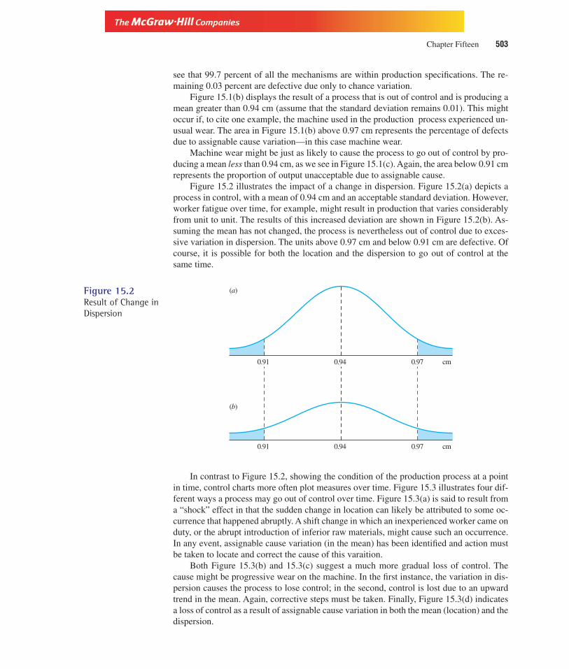
Version, Third Edition
see that 99.7 percent of all the mechanisms are within production specifications. The re-maining 0.03 percent are defective due only to chance variation.
Figure 15.1(b) displays the result of a process that is out of control and is producing amean greater than 0.94 cm (assume that the standard deviation remains 0.01). This mightoccur if, to cite one example, the machine used in the production process experienced un-usual wear. The area in Figure 15.1(b) above 0.97 cm represents the percentage of defectsdue to assignable cause variation—in this case machine wear.
Machine wear might be just as likely to cause the process to go out of control by pro-ducing a mean less than 0.94 cm, as we see in Figure 15.1(c). Again, the area below 0.91 cmrepresents the proportion of output unacceptable due to assignable cause.
Figure 15.2 illustrates the impact of a change in dispersion. Figure 15.2(a) depicts aprocess in control, with a mean of 0.94 cm and an acceptable standard deviation. However,worker fatigue over time, for example, might result in production that varies considerablyfrom unit to unit. The results of this increased deviation are shown in Figure 15.2(b). As-suming the mean has not changed, the process is nevertheless out of control due to exces-sive variation in dispersion. The units above 0.97 cm and below 0.91 cm are defective. Ofcourse, it is possible for both the location and the dispersion to go out of control at thesame time.
Chapter Fifteen 503
Figure 15.2Result of Change inDispersion
0.94 0.97 cm
(a)
0.91
0.94 0.97 cm
(b)
0.91
In contrast to Figure 15.2, showing the condition of the production process at a pointin time, control charts more often plot measures over time. Figure 15.3 illustrates four dif-ferent ways a process may go out of control over time. Figure 15.3(a) is said to result froma “shock” effect in that the sudden change in location can likely be attributed to some oc-currence that happened abruptly. A shift change in which an inexperienced worker came onduty, or the abrupt introduction of inferior raw materials, might cause such an occurrence.In any event, assignable cause variation (in the mean) has been identified and action mustbe taken to locate and correct the cause of this varaition.
Both Figure 15.3(b) and 15.3(c) suggest a much more gradual loss of control. Thecause might be progressive wear on the machine. In the first instance, the variation in dis-persion causes the process to lose control; in the second, control is lost due to an upwardtrend in the mean. Again, corrective steps must be taken. Finally, Figure 15.3(d) indicatesa loss of control as a result of assignable cause variation in both the mean (location) and thedispersion.

Version, Third Edition
15.4 Control Charts for the Mean and DispersionControl charts aid in the detection of assignable cause variation. Different types of controlcharts are formed for at least two variables. The first type, often called an -chart, is de-signed to measure the variation in sample means. The second type measures variation in therange of samples. Logically, it is called an R-chart. A discussion of both types follows.
A. The X�-ChartThe typical -chart is used to measure the variation of sample means around some generallyaccepted level. As Figure 15.4 shows, an upper control limit (UCLX�) and a lower control
X
X
504 Quality Control Techniques
Figure 15.3 Patterns in Means and Dispersion Indicating Loss of Control
(a)Shock effect
cm
Time1 2 3 4 5
(b) cm
Time1 2 3 4 5
(d ) cm
Time1 2 3 4 5
(c) cm
Time1 2 3 4 5

Version, Third Edition
limit (LCLX�) are established around an acceptable measure, which is determined as the grandmean, , of several sample means. The value serves as our estimate of m.
If the sample means fall within the acceptable range, as shown in Figure 15.4, onlychance variation is said to occur. However, if the sample means exceed the UCLX� or fallbelow the LCLX�, the quality control process has detected an assignable cause variation, andthe production process is out of control. The cause for this excessive variation must bedetermined and corrected.
It is customary in quality control procedures to set the UCLX� and the LCLX� three stan-dard errors above and below . This custom results from the empirical rule stating that99.7 percent of all observations in a normal distribution will be within that range.
Thus,
Upper control limit for means
[15.1]
and
Lower control limit for means
[15.2]
However, in practice, is estimated as where is the range of several samplesmeans, and A2 is a constant based on the sample size. Values for A2 can be found inAppendix III, Table O. Using instead of produces similar results and is consider-ably easier to compute. We then find
Upper control limit for means
[15.3]
and
Lower control limit for means
[15.4]
Consider the problem faced by Janet Lugg, director of quality control measures forAT&T. Her plant produces frames for desktop computers which must meet certain size spec-ifications. To ensure these standards are met, Janet collects K � 24 samples (subgroups),each of size n � 6, and measures their width. The results are reported in Table 15.2.
LCLX � X5
� A2R
UCLX � X5
� A2R
3sXA2R
RA2R,3sX
LCLX � X5
� 3sx
UCLX � X5
� 3sx
X5
X5
X5
Chapter Fifteen 505
Figure 15.4An X
–-Chart
1 2 3 4 5 6 7 8 9 10 11
UCLX–
–LCLX
X=
Sam
ple
mea
ns (
X)–
Acceptable rangefor sample means
Samples

Version, Third Edition
506 Quality Control Techniques
Table 15.2Measurements inCentimeters ofAT&T DesktopComputers (K � 24,n � 6)
Sample Sample Measurements X–
R
1 15.2 14.5 15.4 16.5 15.9 16.2 15.6170 2.02 16.2 15.4 15.9 15.2 15.2 14.5 15.4000 1.73 15.6 16.5 15.9 16.2 15.9 16.2 16.0500 0.94 18.5 14.8 15.7 15.2 16.8 14.2 15.8667 4.35 17.5 15.7 14.5 14.2 14.5 15.2 15.2667 3.36 14.3 15.9 16.5 14.8 15.4 14.8 15.2833 2.27 15.4 15.2 15.4 15.8 14.2 15.7 15.2833 1.68 18.0 14.5 14.4 16.2 14.8 16.8 15.7833 3.69 14.2 15.6 14.5 16.1 15.7 15.9 15.3333 1.9
10 15.7 16.5 14.5 14.8 16.8 16.1 15.7333 2.311 14.8 14.5 16.5 14.9 15.8 16.3 15.4667 2.012 16.8 15.8 15.2 15.8 15.7 16.2 15.9167 1.613 15.2 15.9 14.5 15.1 15.9 14.7 15.2167 1.414 15.4 15.7 16.8 15.3 14.8 14.9 15.4833 2.015 18.4 15.7 15.9 14.8 15.5 14.8 15.8500 3.616 16.5 16.8 15.0 15.7 16.9 14.7 15.9333 2.217 15.2 16.9 16.8 17.0 17.1 15.4 16.4000 1.918 16.8 17.2 18.9 18.5 18.5 18.9 18.1333 2.119 13.5 17.6 18.7 21.1 17.2 16.0 17.3500 7.620 19.8 14.5 20.8 19.2 19.2 18.7 18.7000 6.321 18.7 17.9 18.7 20.8 18.4 17.5 18.6667 3.322 17.5 18.0 18.2 20.2 14.2 17.8 17.6500 6.023 14.9 18.9 20.0 16.8 16.2 18.5 17.5500 5.124 18.7 17.9 17.4 18.7 17.2 16.5 17.7333 2.2
� 2.9625
R ��R
K�
2.0 � 1.7 �≥ �2.2
24
� 16.3194
X5
��X
K�
15.6170 � 15.4000 �≥ �17.7333
24
The mean and range for each sample are shown in the last two columns of the table.The grand mean and the mean range are computed. With this information, the UCL andLCL for can be determined. Since each sample size is n � 6, Table O in Appendix IIIreveals A2 to be 0.483. Then
Figure 15.5, which was produced by Minitab, is the control chart for Janet Lugg. No-tice that the means for subgroups 18, 20, and 21 reveal that the process is out of control:The means have increased to levels exceeding the UCL, indicating the presence of as-signable cause variation. Perhaps over time the machines producing the computer partshave suffered unusual wear, resulting in improper performance. Or the variation mighthave been caused by the introduction of inferior raw materials obtained from a new
� 14.89
LCLX � X5
� A2R
� 17.75
� 16.3194 � (0.483)(2.9625)
UCLX � X5
� A2R
X

Version, Third Edition
supplier around the time sample 18 was taken. In any event. Ms. Lugg must locate andcorrect the cause for the unacceptable variation.
B. The R-ChartIn addition to monitoring changes in the mean, it is useful to closely scrutinize variation inthe process. Although the standard deviation is a dependable measure of dispersion, qual-ity control techniques usually rely on the range as an indication in the variability of theprocess. The range is easier to compute, and more readily understood by those without asufficient statistical background.
A lower control limit (LCLR) and upper control limit (UCLR) for the range are calcu-lated; like those for the -chart, they are three standard errors above and below the mean.In principle, they are determined as follows:
Upper control limitfor the range
[15.5]
and
Lower control limitfor the range
[15.6]
where sR is the standard deviation in the sample ranges. However, in practice, it is simplerto use
Upper control limitfor the range
[15.7]
and
Lower control limitfor the range
[15.8]LCLR � D3R
UCLR � D4R
LCLR � R � 3sR
UCLR � R � 3sR
X
Chapter Fifteen 507
Figure 15.5X–-Chart for Janet
Lugg19
0 105 15 2520
18
15
16
17
Sample Number
Sam
ple
Mea
n
LCL = 14.81
UCL = 17.83
X Chart for AT&T Computers
X = 16.32=
–

Version, Third Edition
Values for D4 and D3 are taken from Appendix III, Table O.Using Lugg’s data from Table 15.2, we find
The R-chart shown in Figure 15.6 was generated using Minitab. Notice again that the latersamples indicate the process is out of control: The R-values for samples 19, 20, and 22 ex-ceed the UCL. Action must be taken to identify and correct the source of the assignablecause variation.
LCLR � (0)(2.9625) � 0
UCLR � (2.004)(2.9625) � 5.936
508 Quality Control Techniques
Figure 15.6R-Chart for JanetLugg 8
0 105 15 2520
6
012345
7
Sample Number
Sam
ple
Ran
ge
LCL = 0.000
UCL = 5.93
R Chart for AT&T Computers
R = 2.96–
By examining the - and R-charts, Ms. Lugg determines that the process is out of con-trol. It is common to use both charts jointly in the effort to detect control problems. Aprocess may exhibit a stable mean that stays within statistical control, but the variationaround that mean, as measured by the standard deviation or the range, is so large that mostunits are defective. For example, a process may be designed to produce units 10 feet inlength. If one-half of them are 5 feet and the other one-half are 15 feet, the desired mean of10 feet is maintained, but none of the units are acceptable—they are all either too long ortoo short. Processes should operate so as to produce both a stable mean and a stable varia-tion. Thus, R-charts and -charts are best used in conjunction.
In fact, it is often suggested that the R-chart should be constructed and interpreted first.Recall that the -chart depends on the range (see Formulas [15.3] and [15.4]). Therefore,if the process variation in dispersion is out of control, the control limits on the -chart havelittle meaning. If the R-chart indicates the process variation is in control, only then does itmake sense to construct and interpret the means chart. Example 15.1 illustrates thispractice.
Example 15.1 In December 1997, GTW Electronics, a small manufacturing firm in New Jersey, an-nounced its intention to compete directly with General Electric in the manufacturing ofcertain electrical components. The CEO for GTW called for quality control checks de-signed to measure the variation in the weight of one of the components. Samples of sizen � 6 were taken each hour for K � 5 hours. The results, in ounces, are tabulated here. Ifthe control study suggests unacceptable variation, the CEO has issued a standing order thatthe production process be interrupted until the assignable cause is identified and corrected.
XX
X
X

Version, Third Edition
Hour (A.M.) 1 2 3 4 5 6 R
8:00 4.9 4.8 4.8 5.1 6.6 5.2 5.23 1.89:00 6.8 5.1 5.2 7.1 5.3 5.2 5.78 2.010:00 7.1 6.9 5.9 6.2 6.9 6.9 6.65 1.211:00 6.8 6.2 6.5 7.1 7.6 6.8 6.83 1.412:00 6.0 4.6 4.5 4.5 4.3 5.2 4.85 1.7
29.34 8.1� 5.87
R� � 1.61
Although K � 5 is likely insufficient (recall, it is suggested that K � 20), its use willsimplify the arithmetic in the illustration.
Solution:
Thus, the R-chart appears as� 0
� (0)(1.62)LCLR � D3R
� 3.25
� (2.004)(1.62)UCLR � D4R
X5
X
Chapter Fifteen 509
1 2 3 4 5
UCLR–
R–
1.62
3.25
1 2 3 4 5
UCLX–
–LCLX
X=
5.86
5.08
6.64
Since the R-chart suggests the variation in R is in control, the -chart can be con-structed to test for variation in means.
The -chart becomesX
� 5.09
LCLX � X5
� A2R
� 6.65
� 5.87 � (0.483)(1.62)UCLX � X
5� A2R
X
Sam
ples

Version, Third Edition
Interpretation: It can be seen that the process is out of control. The means for samples 3 and 4 exceed theUCL. The production process should be interrupted and the assignable cause identified andcorrected.
1. Seven samples of size 5 each were taken for the pounds per square inch contained inpressurized containers. Does it appear that the system is out of control based on -charts and R-charts?
Sample
1 2 3 4 5 6 7
25.00 35.00 22.00 24.00 27.00 21.00 31.0029.00 31.00 29.00 30.00 19.00 23.00 30.0027.00 29.00 27.00 31.00 18.00 22.00 21.0031.00 27.00 24.00 21.00 27.00 25.00 22.0027.00 25.00 20.00 26.00 20.00 35.00 31.00
2. The tensile strength for wire is measured in pounds by taking 10 samples of size 4 each. Testfor statistical control using an -chart and an R-chart.
Sample
1 2 3 4 5 6 7 8 9 10
10 19 14 18 8 15 23 18 21 192 18 12 19 9 17 15 17 18 21
15 21 10 14 6 18 14 15 15 2213 23 9 15 6 14 16 15 14 14
3. Five samples of size 7 are chosen, yielding
and
Determine the upper and lower limits for an -chart and an R-chart. Is the process in control?
4. Rector Public Accounting concluded that completion times for audits should be fairly standard.Ten audits are selected for all five of Rector’s storefront offices. Based on the results shownhere, construct and interpret the appropriate control charts to determine whether completiontimes are in control.
Sample
1 2 3 4 5
4.10 10.50 9.70 7.80 15.703.20 15.00 11.90 9.50 8.903.60 6.00 12.00 6.90 7.805.60 9.00 5.80 5.80 7.606.30 8.00 6.90 4.80 6.805.20 5.60 14.80 7.20 5.906.70 3.90 21.80 15.30 3.609.90 7.20 10.90 14.20 5.808.70 5.50 10.80 15.90 4.108.80 6.80 12.80 13.60 5.60
X
R1 � 1.5 R2 � 1.7 R3 � 1.9 R4 � 1.2 R5 � 1.1
X1 � 6.2 X2 � 7.3 X3 � 8.1 X4 � 7.2 X5 � 6.3
X
X
510 Quality Control Techniques
Section Exercises

Version, Third Edition
15.5 Control Charts for AttributesThe control charts for and R are designed to monitor quantitative data in a process. Inmany cases it is necessary or desirable to measure the quality of a process, or the output ofthat process, based on the attribute of acceptability. This statistical procedure determineswhether a process is acceptable based on the proportion and number of defects. Two com-mon types of control charts focus on acceptability: p-charts measure the proportion ofdefects, and c-charts record the number of defects per item.
A. p-ChartsIn constructing p-charts, we simply take note of the proportion of defective items in a sam-ple. This proportion, p, is
As with control charts for variables, we take several samples, yielding several values for p.The mean proportion of defects for these several samples, , is then calculated as
The value serves as our estimate of p, the population proportion of defects, in the eventp is unknown.
The standard deviation of the proportion of defects is
Standard deviation for proportion of defects [15.9]
In the likely event that p is unknown, sp is estimated by sp, where
Standard deviation for proportion of defects when s is unknown
[15.10]
Recall from our discussion of the binomial distribution that the detection of defects isbased on the Bernoulli processes.
Upper control limits (UCLp) and lower control limits (LCLp) are formed three stan-dard deviations above and below the population of defects. If p is known,
Upper control limitfor proportions [15.11]
� p � 3�p(1 � p)n
UCLp � p � 3sp
sp � �p(1 � p)n
sp � �p(1 � p)n
p
p �Total number of defects in all samples
Total number of all items inspected
p
p �Number of defects in a sample
Sample size
X
Chapter Fifteen 511

Version, Third Edition
and
Lower control limitfor proportions [15.12]
If p is unknown,
Upper control limitfor proportions [15.13]
and
Lower control limitfor proportions [15.14]
Opus, Inc. makes electric guitars and other musical instruments. A quality control pro-cedure to detect defects in the company’sAuditory Annihilator model 1000 guitar entailedthe selection of K � 15 different samples of size n � 40. The number of defects in eachsample is shown in Table 15.3. A total of (15)(40) � 600 guitars is inspected.
� p � 3�p(1 � p )n
LCLp � p � 3sp
� p � 3�p(1 � p )n
UCLp � p � 3sp
� p � 3�p(1 � p)n
LCLp � p � 3sp
512 Quality Control Techniques
Table 15.3Defects in K � 15Samples of Size n � 40
Number of Number ofSample Defects p Sample Defects p
1 10 0.250 9 13 0.3252 12 0.300 10 15 0.3753 9 0.225 11 17 0.4254 15 0.375 12 3 0.0755 27 0.675 13 25 0.6256 8 0.200 14 18 0.4507 11 0.275 15 17 0.4258 11 0.275
211
With these data, a quality control specialist for Opus finds
� 0.3517
p �211
600

Version, Third Edition
Then
A preliminary control chart is formed from these findings, as in Figure 15.7, whichwas produced using Minitab.
� 0.1252
LCLp � p � 3�p(1 � p)n
� 0.5782
� 0.3517 � 3�(0.3517)(0.6483)40
UCLp � p � 3�p(1 � p)n
Chapter Fifteen 513
Figure 15.7p-Chart for Opus,Inc.
0 105 15
0.6
0.1
0.0
0.2
0.3
0.4
0.5
0.7
Sample Number
Prop
ortio
n
LCL = 0.1252
UCL = 0.5782
P-Chart for Opus, Inc.
P = 0.3517
Samples 5 ( p � 0.675), 12 ( p � 0.075), and 13 ( p � 0.625) are clearly out ofcontrol. The search for the assignable causes revealed that sample 5 was taken during atime when certain key personnel were on vacation, and less skilled employees wereforced to fill in. The unusually low proportion of defects for sample 12 resulted from aone-time use of superior raw materials when the regular supplier was unable to provideOpus with the usual materials. Sample 13 was taken when new construction at the planttemporarily interrupted electric power, thus disallowing the use of computerized produc-tion methods.
The assignable cause has been identified for each anomaly. If desired, action can betaken to prevent their reoccurrence. Opus may, for example, ensure that in the future keypersonnel stagger their vacations to prevent a repeat of sample 5.
You might presume that an LCLp would not be a concern, since low rates of defects aredesirable. However, unusually low values for p might aid in identifying ways in which de-fects can be minimized. For example, Opus may want to consider regular use of the supe-rior raw materials obtained in sample 12 if they are not cost-prohibitive. Perhaps a studyshould be done to compare the effect on profits of using the higher-grade raw materials.Furthermore, exceptionally low p-values can indicate a problem in that the quality controlprogram is simply not effectively detecting defects.

Version, Third Edition
Example 15.2 The Home Mortgage Company processes home loans for central Illinois residents.Mr. Mooney, president of the company, has been alerted by a new loan officer that severalmistakes in loan applications have not been detected by the employees who must providefinal approval of the loan. Since such carelesness could prove very costly, Mr. Mooney se-lects 25 samples of appplications that have received approval. Each sample has 50 appli-cations. Upon personally reviewing each application, Mr. Mooney finds that each samplecontains applications that should not have been accepted. He records the number of theseapplications for each sample. Based on his findings, Mr. Mooney asks you to construct ap-chart and to comment on the results.
Number of Applications Number of ApplicationsSample with Errors Proportion Sample with Errors Proportion
1 8 0.16 14 5 0.102 12 0.24 15 6 0.123 2 0.04 16 8 0.164 5 0.10 17 7 0.145 6 0.12 18 7 0.146 6 0.12 19 6 0.127 15 0.30 20 9 0.188 8 0.16 21 8 0.169 7 0.14 22 15 0.30
10 7 0.14 23 6 0.1211 5 0.10 24 6 0.1212 21 0.42 25 8 0.1613 23 0.46 216
Solution: The total number of applications that were in error is 216, and the total number of applica-tions that were reviewed is 25 � 50 � 1,250. Therefore, . Theupper limit is found as
The lower limit is
This is shown in the accompanying p-chart
� 0.0124
LCLp � 0.1728 � 3�(0.1728)(0.8272)50
� 0.3332
UCLp � 0.1728 � 3�(0.1728)(0.8272)50
p � 216�1,250 � 0.1728
514 Quality Control Techniques
0 105 15 20 25
0.1
0.0
0.2
0.3
0.4
0.5
Sample Number
Prop
ortio
n
LCL = 0.0124
UCL = 0.3332
P = 0.1728
Version, Third Edition
Any of the samples with more than 33.32 percent of the applications or less than 1.24 per-cent of the applications in error indicate that the approval process is out of control.
Interpretation: Samples 12 and 13 reveal that the process is out of control. Mr. Mooney should consideractions to improve the way in which loans are reviewed for approval.
B. c-ChartsA second type of attribute control chart is the c-chart, designed to detect the number ofdefects in a single unit. In developing a p-chart, an entire unit was deemed either defectiveor not defective. In many instances, however, the presence of one or more defects may notrender the unit unacceptable. A manufacturer of furniture may find several minor defects ina sofa and yet not consider it unacceptable. If the defects per 100 square yards of floorcovering were few and minor, the manufacturer may decide to sell it despite the flaws. Ac-chart is used to analyze the number of flaws per unit of output.
The c-chart is concerned with the number of occurrences (defects) per unit (per sofa orper 100 square yards). This consideration fits a Poisson distribution.
Control limits are established around the number of defects in the population, c. In thelikely event c is unknown, it is estimated by , the mean number of defects in the units.
A unit may consist of a single item, such as a sofa or a 100-square-yard piece of car-pet, or it might contain, for example, a shipment of 50 printed pages in which typos are de-tected. The unit must be consistent in size, number, or area. Earlier we defined the standarddeviation of the number of occurrences as the square root of the mean number of occur-rences. Thus,
Standard deviation forthe number of defects
[15.15]
The control limits are three standard deviations above and below
Upper control limit forthe number of defects
[15.16]
and
Lower control limit forthe number of defects
[15.17]
International Paper inspected 20 sheets of a new type of gift wrap for defects. Theresults are shown in Table 15.4. A c-chart is to be constructed.
� 2.757
sc � �7.6
� 7.6
c �152
20
LCLc � c � 3sc
UCLc � c � 3sc
c.
sc � �c
c
Chapter Fifteen 515
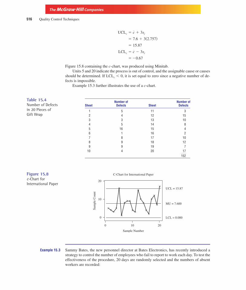
Version, Third Edition
516 Quality Control Techniques
Figure 15.8 containing the c-chart, was produced using Minitab.Units 5 and 20 indicate the process is out of control, and the assignable cause or causes
should be determined. If LCLc � 0, it is set equal to zero since a negative number of de-fects is impossible.
Example 15.3 further illustrates the use of a c-chart.
� �0.67
LCLc � c � 3sc
� 15.87
� 7.6 � 3(2.757)
UCLc � c � 3sc
Table 15.4Number of Defectsin 20 Pieces of Gift Wrap
Number of Number ofSheet Defects Sheet Defects
1 5 11 32 4 12 153 3 13 104 5 14 85 16 15 46 1 16 27 8 17 108 9 18 129 9 19 7
10 4 20 17152
Figure 15.8c-Chart forInternational Paper
0 10 20
10
0
20
Sample Number
Sam
ple
Cou
nt
LCL = 0.000
UCL = 15.87
C-Chart for International Paper
MU = 7.600
Example 15.3 Sammy Bates, the new personnel director at Bates Electronics, has recently introduced astrategy to control the number of employees who fail to report to work each day. To test theeffectiveness of the procedure, 20 days are randomly selected and the numbers of absentworkers are recorded:

Version, Third Edition
Day Number of Absences Day Number of Absences
1 6 11 52 3 12 63 3 13 54 5 14 85 2 15 76 0 16 57 5 17 68 12 18 39 0 19 5
10 0 20 692
Mr. Bates must construct a c-chart to evaluate the new system.
Solution: Since a total of 92 employees were absent over the 20-day period,Then,
and
Since the number of employees who fail to report cannot be a negative value, the UCLc be-comes 0. The occurrence of any days with more than 4 employees absent indicates the sys-tem is out of control. The c-chart shown here summarizes the results of the test.
� � 2.01
LCLc � 1.02 � 3�1.02
� 4.05
UCLc � 1.02 � 3�1.02
c � 92�90 � 1.02.
Chapter Fifteen 517
0 10 20
10
5
0
Sample Number
Sam
ple
Cou
nt
LCL = 0.000
UCL = 4.055
MU = 1.022
Interpretation: On 13 of the 20 days the number of absent employees was excessive. Action must be taken.
5. A manufacturer takes 16 samples of size 25 each and finds the number of defects to be 5, 8, 9,6, 5, 4, 7, 5, 8, 2, 5, 8, 9, 8, 7, and 5. Construct a p-chart and comment on whether the produc-tion process is out of control.
6. MedTec produces aspirin and other over-the-counter drugs. The company’s bottling require-ments certify that between 98 and 104 aspirin tablets must be in each bottle. Twelve samples
Section Exercises
Version, Third Edition
of 200 bottles each are selected. The number of bottles in each sample that do not meet pro-duction specifications is given below. Is MedTec’s bottling process in control?
Number of bottles in each sample that does not contain the proper number of pills:
35, 36, 21, 10, 49, 52, 36, 36, 25, 24, 26, 15
7. The sample proportions of cellular telephones produced by ComWorld that do not meet gov-ernment regulations were found to be, in percentages, 44, 24, 30, 40, 38, 36, 26, 34, 30, 18,24, 34, and 36. Each sample contained 50 cell phones. Construct and interpret the proper con-trol chart. Should ComWorld take action to place its production process back in control?
8. Moroccan Export in Casablanca selects 25 Persian rugs and finds the number of defects perrug shown below. Construct the proper control chart and comment.
Number of Defects per Rug
2 6 3 5 810 3 6 6 45 8 6 9 45 2 5 6 66 5 9 4 5
9. Green Leaf Nurseries sells trees to suburbanites who like to rake leaves out of their lawnsevery fall. After spraying a chemical treatment to kill parasites, Green Leaf selects 20 treesand finds the following number of bugs and other undesirable critters on each tree. Based onthe proper control chart, is the spraying process out of control? Comment.
Number of Parasites per Tree
23 10 9 5 8 9 2514 10 9 6 8 9 1520 6 5 8 6 12
10. Ole Town Press publishes a small newpaper every week in upstate Maine. The editor of thepaper, Kent Clark, is concerned about what he fears is a growing number of typographical er-rors. Mr. Clark randomly selects 15 newspapers over the last several months and finds thenumber of “typos” per paper to be:
2 6 3 5 91 0 5 6 83 2 4 5 6
Does Mr. Clark have to worry that the printing process is out of control?
15.6 Interpreting Control ChartsHow can control charts be used to monitor a process? How can we tell if a system is not incompliance with production specifications? Does the occurrence of only one or two pointsoutside the upper or the lower control limit suggest the process is out of control? Severalfactors must be considered in answering these questions.
Of course, the first and most basic consideration in reading a control chart is whetherany data points fall outside the upper or lower control limits. If even a single point falls out-side the limits, there is statistical evidence that the process is out of control. However, thisis not necessarily cause for great alarm. This one occurrence may simply be due to chancevariation. As much information as possible should be gathered about the possible cause or
518 Quality Control Techniques

Version, Third Edition
causes of this anomaly, and a determination should be made whether a problem really doesexist in that an assignable cause variation can be identified.
In addition, even if all points are within the control limits, the detection of certain pat-terns may signal a serious problem. If, for example, a large number of points are on onlyone side of the center line, the analyst should consider the cause for such a configuration.If the shift to one particular side of the center line appears to have happened abruptly, thecause might be assigned to a sudden change in the use of raw materials or to the introduc-tion of a new training system for incoming employees. If the shift seems to be occurringgradually, evidencing a trend over time, this might indicate that the machinery used in theproduction process is becoming continuously worn and not performing to specifications. Ifan assignable cause can be identified, corrective action can be taken. In general, even if allpoints are within the control limits, there should still be a random fluctuation above andbelow the center line.
Keep in mind that the control limits are established at three standard deviations aboveand below the center line. According to the empirical rule, 99.7 percent of all the observa-tions should be within these limits. Thus, less than 0.5 percent should fall outside the UCLand the LCL by mere chance. If the system is in control, very few, if any, of the pointsshould be out of the established limits.
Furthermore, the empirical rule points out that 95.5 percent of all the observationsshould be within two standard deviations of the center line. That is, 95.5 percent of the datapoints should fall within the first two-thirds of the area around the center line. Only about4.5 percent should deviate from the center line by more than two standard deviations. Thus,even if all the data points are within the control limits of three deviations, but an inordinatenumber are more than two standard deviations from the centerline, action should be takento explain this departure from what the empirical rule states.
This is shown in Figure 15.9. The UCL and the LCL are within 3s of the centerline.This area should contain 99.7 percent of the data points. The first two-thirds of that areaabove and below the center line is within 2s of the center line and should encompass 95.5percent of the data points. In Figure 15.9, for example, although no data points fall outsidethe control limits, a problem may still exist, since so many points are in the area beyondtwo standard deviations from the center line.
Chapter Fifteen 519
Figure 15.9A Control ChartEvidencing Lack ofCompliance
LCL
center line
UCL
3σ
3σ2σ
2σ

Version, Third Edition
15.7 Acceptance SamplingDecisions must often be made regarding the acceptability of an entire lot or shipment ofgoods. A firm may purchase raw materials from its supplier without complete knowledgeof the quality of those materials. It must then test the shipment to determine whether thematerials meet certain minimum specifications. Rarely does a firm examine every item ina shipment. Such a process would be too time-consuming and costly. Instead, a sample isselected to determine whether the entire shipment should be accepted or returned to thesupplier.
During production a manufacturing firm often inspects several unfinished units to de-termine whether production should continue, or whether the semifinished units should bescrapped and procedures reviewed to determine the cause for excessive defects. This deci-sion also involves the use of samples in deciding whether minimum standards are beingmet. This practice is called acceptance sampling.
Acceptance Sampling A sample of a shipment or production lot is examined to de-termine whether it meets certain minimum quality specifications and is thereforeacceptable.
Acceptance sampling is an important and integral part of quality control measures.Decisions regarding the acceptability of materials have a significant bearing on the firm’srevenue and cost structure.
Ensuring that a part fits production standards is crucial to the overall manufacturingprocess. Whether the manufacturing firm produces the part or obtains it from a supplier,specific production standards must be met. If a manufacturer of compact disk systems usesa part that is too small, the entire system may not function properly. If an aircraft assem-blage company relies on a metal that is too heavy or unable to withstand minimum stress,a serious consequence is likely. Obviously, quality control decisions concerning productionspecifications are critical.
Consider a firm making cellular telephones. It obtains a critical part for each phonefrom a supplier in Chicago. The parts are shipped in lots of several hundred. The firm can-not test each part received, so acceptance sampling is necessary. The firm is willing to ac-cept a maximum of 5 percent defective parts in each shipment. This number is called theacceptance quality level (AQL). The firm also limits to 1 percent those shipments thatmeet the AQL but are mistakenly rejected. This has the effect of constraining the numberof nondefective shipments that are discarded.
In common practice, decisions regarding these percentages are most often determinedon the basis of company policy, often in agreement with the supplier. If a less judgmentalapproach is desired in arriving at proper percentages, the Military Standard Sampling Pro-cedures and Tables for Inspection by Attributes (MIL-STD-105D) can be used. These ta-bles specify the proper sample size and number of defects necessary to reject the shipment.
Since sampling is involved, it is possible to make an error in deciding whether to ac-cept or reject a shipment. A shipment that meets the minimum specifications might be re-jected. This is a Type I error, and is called producer risk, because producers run the risk ofhaving a good shipment returned to them.
Producer Risk The probability that sampling error will cause a buyer to mistakenlyreject a shipment and return it to the seller is a producer risk. This is called a Type I error.
520 Quality Control Techniques

Version, Third Edition
A Type II error occurs when a bad shipment is accepted. Accepting a bad shipment iscalled consumer risk, since the buyer would unknowingly retain a shipment with an ex-cessive number of defects.
Consumer Risk The probability that sampling error will lead the buyer to retain ashipment that contains a disproportionate number of defects is a consumer risk. Thisis called a Type II error.
A Type I error is called the a-level, and the probability of a Type II error is called b.Consider again the cellular phone company. It was stated that a shipment containing
more than 5 percent defects should be rejected (AQL � 5 percent), and only 1 percent ofthe good shipments would be erroneously returned (a � 1 percent). This 1 percent is thevalue of the producer’s risk. Its purpose is to protect the firm’s suppliers from unwarrantedrejection of a good lot or shipment.
Recall from our earlier discussion of probability distributions that a hypergeometricdistribution could be used to determine the probability that a certain number of defectswould be found in a shipment. In practice, the binomial distribution, due to its simplicity,is more often used to provide an accurate approximation.
Assume that from several hundred parts received by the cellular phone company, asample of n � 50 is taken. Given that the firm agrees to an AQL of 5 percent, p is set at0.05. It is then necessary to determine what number of defects ensure that no more than 1percent of the good shipments are rejected. That is, what number of defects will ensure thatat least 99 percent of the good shipments containing 95 percent (1.00 � AQL) nondefectsare accepted? This number of defects which determines whether to accept the shipment iscalled the acceptance number.
Acceptance Number The acceptance number is the maximum number of defectsout of a sample that can occur without rejection of the shipment. It ensures that theAQL is maintained without rejecting more than some prescribed percentage of goodshipments.
The maximum number of defects, C, can then be found in the extension to Table C(Appendix III). For n � 50, move down the column headed by p � 0.05 until you find thefirst value that exceeds 1.00 � producer’s risk, here 1.00 � 0.01 � 0.99. This value is0.9968, which is associated with C � 7. The closest probability not exceeding 1 percentdefects is 1.00 � 0.9968 � 0.0032 � 0.01. If there are more than C � 7 defects out of asample of n � 50, the entire lot should be returned.
Example 15.4 Claude and Carol’s DilemmaClaude Vaughan is director of quality control at the PepsiCo bottling plant in Cincinnati.Data on production levels show that an inordinate number of bottles are underfilled. Fear-ing that shipment of the bottles could drive away customers, Claude proposes an accep-tance sampling plan to minimize underfill shipments without causing too many bottles thatare properly filled to be discarded.
He agrees with the production supervisor, Carol Henning, that they can ship a maxi-mum of 1 percent underfills. This represents the acceptable level of defects, soAQL � 1 per-cent. Carol insists that not more than 10 percent of the acceptable production lots should be
Chapter Fifteen 521

Version, Third Edition
rejected. That is, the producer’s risk should be limited to 10 precent. If samples of 100 aretaken from a production run, what is the acceptance number of underfills Claude and Carolcan tolerate before the entire run must be rejected?
Solution: Using the extension of the cumulative binomial table, p is set equal to the AQL of 1 per-cent. Claude and Carol must find the number of underfills that would not result in the re-jection of more than 10 percent of the good production runs. They select a sample of 100bottles from the most recent run. Given p � 0.01, the number of underfills that ensuresthat no more than 10 percent of the good runs are rejected is that value of C with a proba-bility that exceeds 1.00 � producer’s risk, or 1.00 � 0.10 � 0.90. In the table under n �100, find the column headed p � 0.01. Travel down the column until you find a probabil-ity in excess of 0.90. This value is 0.9206, which carries an acceptance number of C � 2.
Interpretation: By rejecting all production runs from which samples of n � 100 were taken that containmore than two underfills, Claude and Carol will ensure that, over the long run, productionruns will not contain more than 1 percent underfills and that runs with less than 1 percentunderfills will be rejected no more than 10 percent of the time.
A. Different Sampling PlansAcceptance sampling assumes that only one sample is taken. This, logically, is referred toas a single-sample plan. However, two or more samples can be taken. Such plans aretermed multiple, or sequential, sampling plans.
A double-sampling plan involves selection of a primary sample. On the basis of theresults of this first sample, the plan then calls for one of three actions: (1) the lot may be re-jected: (2) the lot may be accepted: or (3) a second sample may be taken. Two values of Care specified, where C1 is the acceptance number for the first sample, and C2 is the accep-tance number for both samples.
To illustrate, assume a double-sampling plan stipulates n1 � 100, n2 � 100, C1 � 3,C2 � 8. A preliminary sample of 100 is selected. If three or fewer defects are found, the lotis accepted. If 3 � 8 � 11 or more are found, the lot is rejected. If the first sample contains4 to 10 defects, a second sample of n2 � 100 is taken. If the total defects in both samplesexceed 11, the lot is rejected.
Sequential plans tend to be more efficient than single-sampling plans in that fewer ob-servations are needed to ensure the same degree of accuracy. Sequential plans are oftenused when testing requires the destruction of each unit.
As competition stiffens in the world market, a firm must ensure that its product or ser-vice meets minimum standards if it expects to stay in business. Hence, quality controlmesures are vital.
B. Operating Characteristic CurvesThose involved with quality control plans often find it convenient to construct operatingcharacteristic (OC) curves. These curves display the probability of acceptance under a va-riety of conditions. Specifically, an OC curve can allow the quality control specialist to as-certain, given different values for the proportion of defects p, the likelihood of accepting alot given (1) the size of the sample n, and (2) the maximum number of allowable defects, C.
To illustrate, a sampling plan may be devised in which n � 10 units are routinely cho-sen from each shipment on a random basis. It is determined that if C � 3 or fewer units, theentire lot will be accepted. Under this scheme, it is possible to calculate the probability of
522 Quality Control Techniques

Version, Third Edition
acceptance for different values of p. For example, if, typically, p � 5 percent of the unitsare defective, what is the probability that a given lot will be accepted? This question can, ofcourse, be answered with the use of the cumulative binomial distribution. From the cumu-lative binomial table, it can be seen that the probability of acceptance
If, on the other hand, the proportion of defects in the past has provedto be 10 percent, the probability of acceptance becomes 0.9872. Notice, logically, that the higher the value for p, the less likely it is that the ship-ment will be accepted. If other possible values for p are selected, the relationship betweenp and the probability of acceptance can be determined and depicted by an OC curve asshown in Figure 15.10.
P(C 3}n � 10, p � 0.10) �p � 0.05) � 0.9990.
� P(C 3}n � 10,
Chapter Fifteen 523
Figure 15.10An OperatingCharacteristic Curvefor n � 10, C � 3
Prob
abili
ty o
f ac
cept
ance
π0.0 0.2 0.4 0.6 0.8 1.0
1.0
0.8
0.6
0.4
0.2
0.0
The shape of the OC is determined by the p-value, but other factors also affect it. If,for example, C is increased, the probability of acceptance goes up for any value of p. Thus,the entire OC curve would shift upward.
If the sample size n were increased, the entire curve would shift downward. We have, and . The
likelihood that a larger sample will result in acceptance, given values for C and p, issmaller than that for a smaller sample with corresponding values for C and p. In this man-ner an OC curve can be used to tailor a quality control plan to the specific needs of anybusiness operation.
Solved Problems1. Finding the Fault for Defaults Business Week described the problem a major bank in
Chicago had with load defaults. Assume that samples of size 5 for seven officials were selected,and the results tabulated. Develop an -chart and an R-chart for the bank.
Loan Amount (in $1,000’s)
Official 1 2 3 4 5 X� R
1 14.2 9.2 7.1 6.8 6.0 8.7 8.22 45.5 65.5 45.2 55.2 55.1 53.3 20.33 23.4 31.2 36.3 31.5 32.6 31.0 12.94 32.3 31.2 29.1 27.8 28.1 29.7 4.55 56.7 65.3 45.2 55.5 58.2 56.2 20.16 89.7 90.2 84.2 85.5 89.2 87.8 6.07 112.0 99.2 115.3 98.5 153.2 115.6 54.7
� 54.6 382.3 126.7
R–
� 18.1X5
X
P(C 3}n � 15, p � 0.10) � 0.9444P(C 3}n � 10, p � 0.10) � 0.9872

Version, Third Edition
Solution:
� 44.16
LCLX � X5
� A2R
� 65.04
� 54.6 � (0.577)(18.1)
UCLX � X5
� A2R
524 Quality Control Techniques
1 2 3 4 5 6 7
UCL = 65.04
LCL = 44.16
X = 54.6=
Sam
ple
mea
ns
Samples
There is apparent inconsistency in the size of loans granted by the seven bank officers.Perhaps some effort should be made to find an explanation for the disparity in the officers’practices. The first, third, and fourth officers are granting unusually small loans, and the lastofficer seems to extend exceedingly large loans.
The R-chart is found as
� 0
� (0)(18.1)
LCLR � D3R
� 38.3
� (2.115)(18.1)
UCLR � D4R
1 2 3 4 5 6 7
UCL = 38.3
LCL = 0
R = 18.1–
Samples
Only one officer seems to violate the control limits for the range. Again, the pattern ofthe seventh officer stands out from the rest, suggesting that his or her practices should bereviewed.

Version, Third Edition
2. A Comparison of the Officers Considering the disparity in the officers’ performances, itmight be wise to use a p-chart to compare each officer. Samples of 10 loans by each officer areselected, and the proportion of loan defaults for each is recorded.
Number of Defects ProportionOfficer (defaults), c of Defects, p
1 4 0.42 3 0.33 3 0.34 2 0.25 0 0.06 3 0.37 8 0.8
23
p– � � 0.33
Solution:
We find that 0.498 and 0.162 are the preliminary limits for p and are shown on the p-chart. Thelast officer is again differentiated from the rest. His or her rate of default is excessive. Further,the fact that the fifth officer had no defaults might also indicate a trouble spot. He or she is per-haps being too conservative in extending loans, and a greater degree of aggressiveness mightbe called for.
By eliminating the fifth and seventh samples, we can determine final limits. These areUCLp � 0.495 and LCLp � 0.105.
� 0.162
LCLp � p � 3�p(1 � p )n
� 0.498
� 0.33 � 3(0.056)
UCLp � p � 3�p(1 � p)n
23�70
Chapter Fifteen 525
1 2 3 4 5 6 7
UCL = 0.498
UCL = 0.495
LCL = 0.105LCL = 0.162
LCL = 0
p = 0.33–
Samples
Prop
ortio
ns
A further examination of the loan process might involve the use of c-charts to control forthe number of errors (defects) made in each loan application (unit). In this effort, n � 12 loansare randomly selected, and the number of violations of bank policy for each loan application istallied.

Version, Third Edition
Violations ViolationsLoan (defects), c Loan (defects), c
1 3 7 22 4 8 03 2 9 34 3 10 45 10 11 26 1 12 3
37
In 37 instances bank policy was not followed in extending the 12 loans. Thus,
Then
Only the fifth loan in the sample suggests a problem. Management should determine whoapproved that loan: action can then be taken to reduce the number of loan defaults.
� �2.3, and is set equal to 0
LCLc � c � 3sc
� 8.33
UCLc � c � 3sc
� 1.75
sc � �3.08
c �37
12� 3.08
526 Quality Control Techniques
1 2 3 4 5 6 7 8 9 121110
UCL = 8.33
LCL = 0
c = 3.08–Def
ects
3. These Scoops or You’re Out Crisp-O Raisin Bran, a major cereal manufacturer, promisesthree scoops of raisins in every box. A box with fewer raisins is considered defective. A cus-tomer of Crisp-O will accept a maximum of only 1 percent defective boxes. Crisp-O agrees tothis quality check, but insists on limiting its producer’s risk to 5 percent. That is, no more than5 percent of the shipments that meet this restriction of containing at least 99 percent of boxeswith three scoops must be rejected. Thus, at least 95 percent of the good shipments must be ac-cepted. From a sample of 100 boxes selected from a large shipment, what is the acceptancenumber of defects that will result in rejection of that shipment?
Since the customer will accept no more than 1 percent defects, the AQL is set at 1 per-cent. From the extension to the binomial table, we must find a number C that will not cause therejection of more than 5 percent of the good shipments. (A good shipment is one that containsat least 99 percent of the boxes with three scoops.) The value of p is set equal to 1 percent.Moving down the column headed by p � 0.01 with n � 100, we find the first number to

Version, Third Edition
exceed 1.00 � producer’s risk, or 1.00 � 0.05 � 0.95, is 0.9816, which is associated withC � 3. Thus, if a sample of n � 100 is taken from a large shipment, and more than threeboxes out of the 100 examined contain less than three scoops, the entire shipment should bereturned to Crisp-O.
List of Formulas[15.3] The upper control limit is the maximum value
a sample mean can take without indicating theprocess is out of control.
[15.4] The lower control limit is the minimum valuea sample mean can take without indicating theprocess is out of control.
[15.7] The upper control limit is the maximum valuea sample range can take without indicating theprocess is out of control.
[15.8] The lower control limit is the minimum valuea sample range can take without indicating theprocess is out of control.
[15.10]The standard deviation of the number ofdefects.
[15.13]The upper control limit is the maximum valuea sample proportion can take without indicat-ing the process is out of control.
[15.14]The lower control limit is the minimum valuea sample proportion can take without indicat-ing the process is out of control.
[15.15] The standard deviation of the number ofdefects in a c-chart.
[15.16] The upper control limit is the maximum num-ber of defects that can occur without indicat-ing the process is out of control.
[15.17] The lower control limit is the minimum num-ber of defects that can occur without indicat-ing the process is out of control.
Chapter Exercises11. The director of your division at your firm happens by your desk and notices that you are
working with something called a control chart. Since he got his job because he is the boss’sson-in-law, and he knows nothing about control charts or quality control, he wants you to de-scribe what you are doing and why you are doing it. Describe in your own words the purposeand function of -, R-, c-, and p-control charts.
12. Define the acceptance number and the acceptance quality level as used in acceptance sam-pling. If AQL is 5 percent and producer’s risk is 1 percent, how would you describe the accep-tance number in terms of these two percentages?
X
LCLc � c � 3sc
UCLc � c � 3sc
sc � �c
LCLp � p � 3�p(1 � p )n
UCLp � p � 3�p(1 � p )n
sp � �p(1 � p )n
LCLR � D3R
UCLR � D4R
LCLX � X5
� A2R
UCL X � X5
� A2 R
Chapter Fifteen 527

Version, Third Edition
13. Acme Salt Mine, where you work as a gofer trainee, has asked you to record the number ofmiles the sales staff drives in making sales calls. Using these data, samples are taken over fiveconsecutive days. From the results shown, construct - and R-charts. Does the system appearout of control?
Miles Driven
Sample
1 112 132 145 117 125 1892 214 252 274 189 236 2033 198 205 185 214 236 1994 236 250 245 210 210 2595 109 111 125 132 145 152
14. Over a period of several days, Tolbart Manufacturing collects seven samples of size 5 on theweight of a new product. Construct an R-chart to determine whether the production process isin control. The weights in ounces are shown here.
Observations
Samples
1 42 48 28 43 522 52 57 24 41 213 48 65 54 35 454 59 35 53 63 565 68 65 62 35 566 57 54 42 32 357 51 51 51 34 35
15. What does an -chart reveal about the process in the previous problem?
16. A producer of snowmobiles samples daily output by taking 10 samples, each of five days’output. The data are shown here. Construct an R-chart and draw a conclusion regarding thecontrol of the process.
Observations
Samples
1 5 3 5 5 52 2 6 1 3 13 6 9 5 6 24 4 8 8 5 125 2 5 9 8 106 5 7 6 9 117 6 4 5 5 168 8 5 4 4 89 9 9 7 7 9
10 5 6 8 8 8
17. Using the data from Exercise 16, construct and interpret an -chart.
18. The lengths of rope measured in feet that are produced by a new technology are shown here.Construct an R-chart and form a conclusion regarding the benefit of this new method ofproduction.
X
X
X
528 Quality Control Techniques

Version, Third Edition
Observations
Sample
1 12.5 14.8 21.5 15.8 23.6 12.52 13.6 15.9 23.6 14.6 25.4 21.53 15.8 26.0 15.6 21.5 21.5 14.24 15.6 8.0 25.7 23.5 19.2 15.65 12.5 26.0 32.8 15.4 19.7 15.56 14.8 15.8 32.5 18.2 18.2 12.57 22.5 16.9 12.8 14.7 14.5 18.28 32.6 14.5 14.9 12.0 15.6 14.59 15.5 14.2 15.8 14.5 21.5 12.2
19. Using the data from Exercise 18, construct and interpret an -chart.
20. Twenty samples of size 7 for the weights (in ounces) of filled cola cans produced the resultsshown here. Must the producer search for assignable causes based on an R-chart or on an -chart?
Sample Mean Range Sample Mean Range
1 27 6 11 32 72 32 8 12 45 93 21 4 13 34 54 24 8 14 23 75 43 6 15 32 86 31 7 16 21 47 23 5 17 34 48 12 6 18 21 79 21 5 19 27 5
10 32 9 20 34 6
21. The results of ten samples of size 6 each for the length (in inches) of electrical cord are shownhere. As measured by an R-chart and an -chart, is the system out of control?
Sample Mean Range Sample Mean Range
1 20 7 6 34 42 18 9 7 21 33 17 8 8 12 24 23 2 9 18 65 19 5 10 13 5
22. The AllRight Insurance Company of Buffalo, New York, collects five samples of size 12 eachof claims filed against them for auto damage. The means and ranges are given here. Construct
- and R-charts, and comment.
Sample Mean Range
Jan $812 $54Feb 234 23Mar 321 27Apr 250 29May 276 20
23. In Exercise 22, what would a heavy snowstorm in January constitute?
X
X
X
X
Chapter Fifteen 529

Version, Third Edition
24. A large auto parts store in Little Rock refuses to accept a shipment of distributor caps if morethan 5 percent are defective. The store managers agree, to protect their suppliers, that in sam-pling shipments they will not return more than 20 percent of all shipments that meet the 5 per-cent requirement. If samples of 50 are taken, what is the acceptance number?
25. For Exercise 24, what is the acceptance number if samples of 20 are taken?
26. In Exercise 24, if the actual percentage of defective caps is 10 percent, what is the probabilitya shipment will be accepted if a sample of 50 caps is taken?
27. From Exercises 24 and 26, if the true percentage of defects is 1 percent, what is the probabil-ity that the shipment will be accepted? Comment on the difference in your answers in thisproblem and in Exercise 26.
28. Kmart sells radar detector units used by motorists. Company policy is to accept a maximumof 5 percent defective units. Only 10 percent of those shipments that contain fewer than 5 per-cent defects will be sent back to the supplier. What is the maximum number of defectivedetectors that can occur in a sample of 50?
29. If producer risk is reduced to 1 percent in Exercise 28, what is the acceptance number? Com-ment on the difference in your answer from Exercise 28.
30. A recent graduate of the MBA program at a small private university is now in business forhimself. He wishes to test his production method by taking 10 samples of size 8 each. Hefinds and . Determine his control limits for both R-charts and -charts.
31. To further test his product, the graduate from Exercise 30 takes 15 samples of size 100, andfinds the number of defects in each sample to be
Sample Defects Sample Defects
1 4 8 82 8 9 73 8 10 94 3 11 35 8 12 96 5 13 67 6 14 8
15 7
If his p-chart reveals his production process to be in control, he plans to “go global” with hisproduct. Should he do so?
32. TCBY Yogurt tested the stability of its franchise operation by taking samples of 25 each in sixstates. The numbers of failed franchises were 4, 7, 2, 6, 8, and 12. Develop a p-chart to helpTCBY monitor its outlets.
33. Bradley University uses two word processing packages: Professional Write and WordPerfect.In a comparison of their relative merits, samples of size 18 are taken for the time required forfaculty and staff to master each package. The results are shown here. Prepare - and R-chartsfor use in evaluating each package. What are your conclusions?
Professional Write v.2.0
Mean RangeSample (hours) (hours)
1 3.2 1.22 3.9 0.93 3.9 1.54 3.7 1.5
X
XR � 17X5
� 42
530 Quality Control Techniques
(Continued )

Version, Third Edition
Professional Write v.2.0
Mean RangeSample (hours) (hours)
5 3.6 1.16 3.3 1.97 2.5 1.88 3.6 1.7
WordPerfect v.5.1
Mean RangeSample (hours) (hours)
1 78.5 10.22 79.5 8.73 55.6 6.84 78.6 7.85 58.9 11.36 72.8 10.67 86.9 12.3
34. In a continued review (see Exercise 33) of the word processing packages, personnel atBradley University took four samples (actually, the number of samples was much greater) of50 pages each typed by WordPerfect and found
10 pages with a total of 12 errors.12 pages with a total of 18 errors.8 pages with a total of 15 errors.
17 pages with a total of 13 errors.
Four samples of 50 pages each typed by Professional Write revealed
2 pages with a total of 2 errors.0 pages with errors.1 page with a total of 1 error.3 pages with a total of 3 errors.
Prepare a p-chart and a c-chart for these data.
35. Up Your Cash Flow (Granville Publications), by Harvey Goldstein, CPA, discusses variouscomputer spreadsheets and the speed with which they can forecast budgets. Lilly Paper Prod-ucts applied some of the principles found in the book. They discovered that 10 samples of size15 of the number of days it took local offices to prepare their quarterly budgets yielded meansand ranges of
Sample Mean Range Sample Mean Range
1 32.4 23.4 6 45.7 34.62 68.7 45.3 7 56.7 17.53 45.6 18.6 8 13.2 12.24 67.6 45.6 9 34.5 29.85 23.8 18.3 10 76.7 67.9
Construct - and R-charts. What can you conclude?
36. Nation’s Business reported that Harvey Mackay’s book, Beware the Naked Man Who OffersYou His Shirt (Morrow), tells business executives, among other things, how to select a lawyer.A large law firm chooses one sample of size 30 each month over the last 15 months of thenumber of legal cases it handled. Recorded are the numbers of those cases that the firm
X
Chapter Fifteen 531

Version, Third Edition
lost: 5, 4, 12, 0, 19, 21, 4, 23, 8, 12, 19, 12, 23, 6, and 10. Construct a p-chart to determinewhether the process is in control.
37. Kador, the world’s most evil scientist, makes amulets to cast evil spells. To control quality,Kador’s assistant, Meldok, selects 30 amulets and inspects each for defects. The purpose ofthe inspection is to determine whether a given amulet contains too many defects to use. Thenumber of defects in each amulet is shown here. Construct the proper quality control tool, anddetermine whether the process is out of control.
Number Number NumberAmulet of Defects Amulet of Defects Amulet of Defects
1 3 11 4 21 82 2 12 2 22 23 4 13 0 23 74 1 14 0 24 35 0 15 5 25 16 1 16 2 26 97 3 17 3 27 78 4 18 4 28 09 0 19 5 29 0
10 3 20 7 30 1
38. A firm that prepares tax returns tries to double-check all forms it completes. However, fromJanuary to April 15, this is often impossible. The firm’s policy is to allow a maximum of 1 per-cent of the returns to contain errors. If more errors are suspected, the entire batch must beredone. However, the firm does not want to redo a batch of returns if fewer than 1 percentcontain errors, if this can be avoided. It decides to set a limit on recalculating a good batch toonly 5 percent of the time. A sample of 20 taken from a large batch reveals five returns havemistakes. Should the entire batch be reworked?
39. Mother’s Best sells doughnut holes retail. From a truckload, a sample of 100 is selected, and 8holes are found to be defective. If Mother’s Best is willing to accept a maximum of 10 percentdefects, and its suppliers want to restrict their risk to 20 percent, should this shipment be sentback?
40. Yakov Smirnoff, a Russian-American comedian, advertises that Best Western has economi-cal rooms for travelers. The cost of a night’s lodging for 15 nights (n � 15) was averaged20 times (k � 20 samples). The mean of those 20 sample means proved to be $45.12, with amean range of $12.34. What are the values for - and R-charts?
41. Budget Rental, a nationwide car rental firm, practices a policy in which each car is putthrough a checklist before it is given to a customer. A recent assessment of 20 cars found thefollowing number of checkpoints had been neglected: 3, 5, 7, 2, 6, 8, 10, 4, 9, 12, 7, 3, 6, 13,12, 4, 15, 4, 5, and 9. Does it appear the checklist system is in control?
42. Bids by a construction firm for a job are monitored to determine whether it might increasethe number of bids the firm wins over its competitors. Samples of size 40 bids are taken,yielding means and ranges shown here in thousands of dollars. Is the bidding process out ofcontrol?
Sample Mean Range
1 7.5 5.42 8.6 4.53 4.5 3.44 5.6 2.55 8.9 3.2
X
532 Quality Control Techniques

Version, Third Edition
43. Suspicious that My Mother’s Catch, a fishing boat in the Bering Sea, is using illegal means toaugment its daily catch, the U.S. Coast Guard takes samples of five boats’ hauls for six daysover the past month. Could unlawful tactics be a possible assignable cause?
Boat Mean Haul (tons) Range
My Mother’s Catch 39.4 12.2Neptune’s Spear 18.6 18.2Salty Dog 19.6 21.2Wind Ablow 38.8 22.5Deep 6 21.2 19.2
44. Fox Pictures distributes many films to its movie theaters throughout the country. It decides tosample batches of a particular film to determine whether copies were reproduced withoutflaws. If the sampling process suggests that no more than 5 percent of the copies have a flaw,the entire lot will be distributed to the movie houses. Officials wish to reject good lots nomore than 10 percent of the time. If they screen 20 copies of a film and find 7 with flaws,should the entire lot be destroyed?
45. In the 20 films Fox screened in Exercise 44, they find the following number of flaws in thefilms: 6, 7, 2, 12, 19, 10, 2, 2, 22, 21, 0, 1, 19, 0, 15, 3, 12, 21, 2, and 5. Does it appear that thereproduction process is out of control?
46. Labor, Inc., selects several samples of size 50 employees for whom it has recently found jobs,and finds that the number in each sample who still have the same job one year later is 10, 12,4, 17, 2, 21, 34, 32, 43, 12, 5, and 5. Is the placement system out of control?
47. Calculate the final control limits in Exercise 46.
48. The IBM 4019 laser printer produces almost 10 pages per minute, on the average. Of 1,200pages printed, 100 are selected at random and examined for errors. Twelve pages are found tohave an average of 2.3 errors. Should the entire 1,200 pages be reprinted if AQL � 5 percentand producer risk is set at 15 percent?
49. Determine the control limits for a c-chart in Exercise 48.
50. Temperatures in refrigeration boxes are monitored over a 10-day period, during which thetemperature is registered every hour for eight hours. The resulting means and ranges areshown. Does it appear that something should be done about the refrigeration process?
Sample Mean (F) Range Sample Mean (F) Range
1 32 29 6 23 212 45 21 7 57 343 12 45 8 13 454 54 34 9 31 125 17 24 10 47 2
51. Federal Express takes eight samples of size 25 for the number of hours it took to deliver pack-ages. The results of that survey are shown here. Need corrective action be taken?
Sample Mean Range Sample Mean Range
1 22.2 3.2 5 24.6 3.32 17.5 3.4 6 23.3 2.43 18.0 2.9 7 21.5 2.44 23.4 2.5 8 19.8 3.1
Chapter Fifteen 533

Version, Third Edition
From the Stage to Real LifeAs the director of product quality at Minot Industries, from the Curtain Call exercise, youare likely to be a member of the American Productivity and Quality Center (APQC). If so,you are able to obtain a wide variety of support from this organization in the conduct ofyour job. A visit to the APQC web site (http://www.apqc.org) will acquaint you with theavailable training seminars and publications that relate to your goals at Minot.
At the home page, click on BENCHMARKING, a way to develop quality standards.At the next page, look at the list of training seminars. Examine several of the offerings andmake a list of some that bear directly on the job ahead of you at Minot. Then go back to theBenchmarking page and scroll through their list of articles and publications. Make a list ofsome that bear directly on the situation at Minot.
Return to the APQC home page and click on the PRODUCTIVITY AND QUALITYarea. Again, think about APQC resources that will help you to succeed in your job at MinotIndustries.
534 Quality Control Techniques
C U R T A I N C A L LRay Murdock, the newCEO for Minot Industries,as mentioned in Setting
the Stage at the beginning of this chapter,has pledged to improve the production stan-dards at Minot. For many years the com-pany has produced glassware of varioustypes. Due to the introduction of more mod-ern production techniques, Minot has suf-fered certain “growing pains” that have re-sulted in an unacceptable reduction in thequality of its product.
To combat this trend, analysts at Minotcollected 5 samples of the weights measuredin grams of the lead that is used to producelarge crystal stemware. The data are recordedhere.
Sample
1 2 3 4 5
5.2 5.8 10.3 4.9 8.96.3 6.8 13.5 9.5 5.87.5 4.5 12.5 6.8 4.77.9 6.8 14.9 8.9 2.98.2 9.5 9.2 2.8 4.53.2 4.5 8.9 4.5 6.28.9 6.5 6.2 6.5 3.5
In addition, 10 samples of sizes 50each are examined and the number of defec-tive units in each sample is found to be 5, 6,10, 15, 2, 5, 19, 3, 0, and 15. Finally, 20 in-dividual glass canisters are randomly cho-sen. Each is inspected and defects for all 20are recorded:
Number of Number ofCanister Defects Canister Defects
1 3 11 52 5 12 63 0 13 34 8 14 25 10 15 86 5 16 87 2 17 78 8 18 59 1 19 2
10 5 20 8
As the director of product quality, it isyour job to construct the appropriate con-trol charts and report your findings in theform of a statistical report as described inAppendix I.

Version, Third Edition
535
A.1 IntroductionAs the business environment grows in its complexity, theimportance of skillful communication becomes essential inthe pursuit of institutional goals. In addition to the need todevelop adequate statistical skills, you will find it necessaryto effectively communicate to others the results of yourstatistical studies. It is of little use to formulate solutions tobusiness problems without transmitting this information toothers involved in the problem-solving process. The impor-tance of effectively communicating the results of yourstatistical study cannot be overemphasized.
Unfortunately, it seems that many business managerssuffer from inadequate communication skills. The Decem-ber 1990 issue of the Training and Development Journalreports that “Executives polled in a recent survey decry thelack of writing skills among job candidates.” A report in a1993 issue of Management Review notes the “liability im-posed on businesses by poor writing skills.” The reportstates that employers are beginning to place greater empha-sis on communication in hiring practices. Many employershave adopted policies requiring job candidates to submit abrief written report as part of the screening process. An Au-gust 1992 issue of Marketing News reveals that “Employersseek motivated communicators for entry-level marketingpositions.” Obviously, the pressing lack of adequate writingand communications skills in American businesses is welldocumented.
Therefore, the purpose of this appendix is to illustratesome of the major principles of business communication andthe preparation of business reports. We examine the generalpurpose and essential features of a report and stress the ben-efits of effective report writing. Emphasis is placed on thecustomary form a business report should take and the for-mat, content, and purpose of its component parts. We willstudy illustrations of practical reports and the problems willprovide the opportunity for students to develop and sharpentheir communication skills.
A.2 The Need to CommunicateMost business decisions involve the cooperation and inter-action of several individuals. Sometimes dozens of col-leagues and co-workers strive in unison to realize mutualgoals. Lines of communication must therefore be maintainedto facilitate these joint efforts. Without communicating ideas
and thoughts it would be impossible to identify commonobjectives and purposes necessary for successful operations.Without communication and the team effort it permits, thesuccessful completion of any important project can be jeop-ardized. Some aspects of the project would be unnecessarilyreplicated while other tasks would be left unattended. Fur-ther, in the absence of adequate communication, colleagueswould find themselves working at cross-purposes andperhaps pursuing opposing goals. What one team membermay have worked to assemble one day, a second team mem-ber may dismantle the next. Without communication thechances for a successful outcome of any business endeavorare significantly reduced.
A.3 The Characteristics of the Reader
Business reports are quite often intended for a wide varietyof different audiences. It is critical that you carefully identifythe intended audience for your report, otherwise it is likelythat your report will be misdirected and less effective. Youshould consider exactly what the readers of your reportalready know and what they need to know to make informeddecisions.
You should also consider the attitude the audience willadopt toward your report. If you fear that the readers maybe somewhat hostile toward your report, you may want tooffer more supporting evidence and documentation thanyou would if their reception was thought to be more favor-able. The educational background and work experience ofthe audience is also a key factor in the formulation of yourreport. A report written for top executives will differ con-siderably from that prepared for line supervisors in terms ofstyle, word usage, and complexity. Even age, gender, andother demographic characteristics might serve to shape thereport.
One thing is certain. Whether you earn your livelihoodas an accountant, a marketing manager, a production super-visor, or a sales representative, you will not work in avacuum. You will find it necessary to constantly commu-nicate with others in order to successfully complete your job.Generally speaking, the larger the institution in which youwork, the greater will be the need to prepare written reports.As the organization grows in complexity, so does therequired degree of formal communication.
A P P E N D I X I
Business Report Writing

Version, Third Edition
A.4 The Purpose ofStatistical Reports
Given the importance of communication, it should come asno surprise that the primary purpose of a report is to conveyinformation. In this effort, statistical reports are fairly conciseand follow a rather predetermined pattern. This familiarpattern permits easy recognition of the essential features andallows the reader to quickly comprehend the study. To com-plete a statistical report you must isolate the problem andcollect the necessary data. The population must be clearlyidentified and a sample carefully chosen. The researcher thenconducts the study and prepares to report the results.
As noted above, the procedure to be followed in com-piling a statistical report consists of rather precise and well-defined steps that may be modified only slightly.Immediately following the title page (which is illustrated inthe example provided later), the statistical report provides anaccount of its conclusions and recommendations. In a busi-ness setting this opening statement is usually referred to asan executive summary. The executive summary, along withthe other parts of a statistical report, are discussed in turn.
A. The Executive SummaryThe intent of the executive summary is to immediatelyprovide the time-constrained reader with the important factsand findings derived from the study. It summarizes thesefindings and conclusions, along with any recommendations,and places them at the beginning of the study. This place-ment provides easy access to the more important informa-tion relevant to any decision that a manager must make. Ifthe manager is interested in any further details, he or shemay consult the main body of the report.
The executive summary should be written in a nontech-nical manner. It is intended for upper-level managers whoseexpertise often lies in business management and not in tech-nical fields such as chemistry, physics, or even, in manycases, statistics. They generally have little concern for thetechnical aspect of the report. They only want to be assuredthat your have considered all relevant business factors andfollowed proper scientific procedures in the formulation ofthe report. If the reader then desires a more complete techni-cal explanation, he or she can read any additional portion ofthe report. The executive summary seldom exceeds one ortwo pages.
Although the executive summary precedes the main re-port when it is submitted in final form, the summary is writ-ten only after the study has been conducted and the rest ofthe report has been completed. The summary should includeno new information not presented in the report, and shouldnot offer conclusions based on data or information not con-tained in the report.
B. IntroductionThe second step is a brief introduction describing the natureand scope of the problem. Any relevant history or back-ground of the problem that is essential to a thorough under-standing and provides clarification for the rest of the studyshould also be included. A statement is made explaining whythe resolution of this issue is important and the critical needto formulate a course of action.
C. MethodologyThe third section of a statistical report is more technical thanthe rest of the study, as it explains the exact nature of the sta-tistical tests that you intend to conduct. It describes in detailthe precise quantitative tools and techniques to be used, andreveals the manner in which they will lead to the desired re-sults. It is also customary to briefly characterize the data setand the manner in which the sample was taken. This will be-come familiar to you as you gain an increased understandingof statistical analysis and its many applications.
The methodology that you use will depend largely onwhat you want to accomplish. This fact too will becomemore evident as you gain more insight into the process ofstatistical analysis as described in this text.
D. FindingsIt is here that the true statistical analysis is performed. Thefindings consist of the actual statistical computations thatprovide the information required to make decisions and rec-ommendations. These calculations may vary from simpledescriptive techniques to the more advanced inferentialanalysis. The computations are shown in sufficient detail toreveal and validate the statistical test without providingneedless information or becoming overly cumbersome.
In addition, comments regarding the computations areprovided to note the results and draw attention to their sig-nificance. That is, the results of the computations are merelycited or quoted. No effort is made to discuss or interpretthese computations. This is left for the next segment.
E. Discussion and InterpretationBased on the findings from the previous section, the re-searcher now offers a discussion and interpretation of the
536 Business Report Writing
Executive Summary A statement of conclu-sions and recommendations that is placed at thebeginning of a report

Version, Third Edition
report’s major implications. The researcher should providean interpretation of the findings in a meaningful and yet non-technical sense. This section has a considerable impact onthe formulation of the solution to the problem described inthe introduction, which motivated the report.
F. Conclusionsand Recommendations
This final segment often repeats some of the informationfound in the executive summary, yet allows the researcherto explain in greater detail how and why the conclusionswere reached. A more complete discussion of the recom-mendations may also be included. It is important that thissection be based on the results of the findings and not offerconclusions or recommendations not supported by theanalysis.
If reports are prepared in this organized form, they areinherently more useful and lend the researcher a sense ofcredibility and authority. The report will command respectfrom those who rely on it to make important decisions.
A.5 Illustrations andExamples
We can form a more complete picture of reports and ab-stracts by using examples from specific case problems. Wewill look first at a full statistical report designed to assist inthe consequential decision regarding location for plantexpansion. Such a decision would likely prompt an entirereport, as opposed to an abstract, due to the cost involvedand the long-term effect of plant location.
Realistically, such a decision would require statisticalanalysis beyond the mere descriptive tools presented here.However, we will approach the issue of plant expansion onlywith the simple descriptive analyses covered in the first twochapters of this text. With this limitation in mind, let usbegin our examination of the report we would submit in ourdecision regarding plant site.
You have just been hired as a management analyst byGlobal Motors, Inc., in Detroit, Michigan. Mr. Sumner, CEOfor GM, has requested that your management division pre-pare a statistical report on the feasibility of constructing anew assembly plant. Under consideration for the site are fourcities: Houston, Detroit, Pittsburgh, and Boston. How wouldyou respond?
After the title page, the report would present theexecutive summary. (Remember, the executive summary,summarizing all the main findings, conclusions, and recom-mendations, is drawn up only after the study has beencompleted.) The title page might appear as:
ALTERNATIVE PLANT SITES
FOR THE 1998 EXPANSION PLAN OF GLOBAL MOTORS
Submitted toSamuel Sumner
Chief Executive OfficerGlobal Motors International
Executive HeadquartersDetroit, MI
Prepared byJarrod Hirsch, Chief
Managerial Analysis DivisionDivisional Branch Headquarters
Global Motors InternationalChicago, IL
August 10, 1998
A. The Executive SummaryThe executive summary could appear as:
Upon careful consideration of all relevant issues, theManagerial Analysis Division recommends that Houstonbe chosen for the new plant expansion site for Global Mo-tors. After thorough review, the Division has found thatHouston offers more of the requisite facilities and ameni-ties for successful completion of the expansion project.
The Division considered factors such as an availablelabor supply with the necessary training or potential fortraining, as well as the prevailing wage rates. We analyzedgeographical access to raw materials. We concluded thatlocal transportation facilities were adequate to accommo-date the shipping volume required by the assembly oper-ations.
Cooperation with local and state governments in theHouston area seems assured. The state attorney general’soffice has offered certain tax incentives that exceed thoseforthcoming from the other potential sites. Further, thecity of Houston has agreed to delay Global Motors’ pay-ment of property and city sales taxes for a period of twoyears. In addition, Texas is a right-to-work state. This isnot the case in those states in which the other proposedsites are located.
Appendix I 537

Version, Third Edition
The Division made a thorough comparison of hous-ing facilities for both managerial and hourly workers. Ourfindings clearly indicate that the Houston market offerssuperior opportunities with reasonable mortgage rates.We also concluded after a complete comparative evalua-tion that the schools in Houston were at least comparableto those in the other potential sites.
It is hereby recommended that a transition team beselected to assist in the relocation of some of our keypersonnel who will temporarily staff the new facilities.An advance team may also be formed to maintain contactwith the proper officials in both public and private organi-zations to facilitate in the completion of the expansionproject.
Notice how the executive summary offers a set of con-clusions based on the findings, and recommendations thatlogically follow from the information contained in the study.Furthermore, effort is taken to ensure that all critical con-cerns have been addressed. Attention was given to factorsranging from business taxes to schooling for the employees’children.
B. IntroductionThe introduction is the next component of the statisticalbusiness report form. Recall that it addresses any relevanthistory and offers clarification as to why the issue needs res-olution.
Since 1990, the production facilities for Global Motorshave been inadequate to maintain pace with the requiredlevel of output. Demand is anticipated to increase in thenear future. Based on these historic and projectedevents, it is essential that a viable plant site be identifiedfor the purpose of expanding Global Motors’ productioncapability.
Unless production facilities can be adequately en-hanced, it is likely that Global Motors’ market share willerode and the firm will be placed at a competitive disad-vantage. Industry studies have shown that GM’s competi-tors have already expanded production capabilities orplan to do so in the near future.
C. MethodologyThe methodology section specifies the tools that will be usedto complete the study. As noted above, since we haveexamined only basic descriptive tools, we will restrict ouranalysis of plant site selection to only these tools. In reality,of course, many other types of tools would be used. This sec-tion also includes a brief description of the data set.
METHODOLOGY:
Various descriptive tools will be applied to the data col-lected for the purpose of conducting this study. Distribu-tion tables, contingency tables, and numerous pictorial
displays will be used to analytically determine theoptimum site for Global Motors’ plant expansion. Each ofthese tools will be applied to the data obtained for all fourcities. The intent will be to provide a basis of comparisonsufficient to permit a conclusive argument as to whichsite is preferable.
Data for several relevant variables have been ob-tained directly from local governments in proposed siteareas as well as from published sources. These sourcesinclude Survey of Current Business and Urban Econom-ics. These data will be used in a comparative analysis ofthe proposed sites.
Notice how this section enumerates and explains themethodology and how each tool will be employed to derivea conclusion.
D. FindingsThis section contains the actual statistical calculations. Itconsists of a presentation comparing all four sites using thevarious descriptive tools. The bar chart will show the tax in-centives in each city, the frequency tables depict the costs ofhouses in each local market, and the contingency tables re-flect the transportation facilities.
The relevant statistics displayed by the descriptiveanalysis are communicated in this section in a formal man-ner. Presume, for example, that the data analysis disclosesthe following:
Table A, which is a frequency table of housing costs for1,000 homes surveyed in Houston, reveals that averagehousing costs are lowest in that city. As shown in thetable, 56 percent of all houses are in the $100,000 to$120,000 range. Pittsburgh offers an average of$120,000.
538 Business Report Writing
Table AFrequency Table forHousing Costs inHouston (in $000’s)
Housing Costs Frequency
60 80 9280 100 115
100 120 560120 140 135140 160 98
1�,�0�0�0�
Chart 1 discloses that Houston offers access to 56percent of all needed raw materials within 24 hours, whilethe other potential sites threaten delays of 72 hours.
Chart 2 for transportation costs in all cities showsthat costs range from an average of $320 per month to$512 per month. The lowest is in Detroit.
Chart 3 for tax incentives shows that total tax sav-ings in Houston should reach $2,000,000. In Detroit,however, the savings were projected to be as low as$500,000.

Version, Third Edition
Notice that in this section no interpretation or signifi-cance is attached to the findings. That is left for the nextsection. In this section the numbers are quoted or cited; thereis only a description or accounting of the data.
E. Discussion and InterpretationThe discussion and interpretation section highlights therelevant findings and offers an explanation. Presume that
from the findings the following discussion and interpretationis possible:
The findings provided by the pie chart for access to mar-kets for raw materials reveals that Houston offers thegreatest accessibility to all necessary materials within24 hours. The other proposed sites average a muchlonger delay. This suggests that costs of transportationwould be higher. Further, production planning would bemore difficult. As shown in the frequency tables, the lower
Appendix I 539
Chart 2Average MonthlyTransportation Costsfor All Cities
Cos
ts (
dolla
rs)
550
500
400
350
300
Houston Detroit Pittsburgh Boston
450
City
Chart 3Tax Saving duringFirst Year ofOperations (inmillions of dollars)
Tax
savi
ngs
2.001.751.501.251.000.750.500.25
Houston Detroit Pittsburgh
City
Boston
24 hours
60 hours
48 hours36 hours
Number of HoursRequired to Receive Percentage of Degrees in
Raw Materials Raw Materials Pie Chart
24 56 360 � .56 � 201.636 24 360 � .24 � 86.448 11 360 � .11 � 39.660 9 360 � .09 � 32.4
3�6�0�.�0�
Chart 1Pie Chart for Accessto Raw Materials inHouston

Version, Third Edition
housing costs in the Houston area mean that wages couldbe kept at a lower level, minimizing labor costs.
Although Pittsburgh reports lower overall housingcosts, the real estate market in Pittsburgh has suffered adownturn recently. If this continues, it may be evidencethat the homes purchased by our employees might proveto be an unfortunate investment.
The stacked bar charts reflect considerable instabilityin city governments in several of the suggested sites. Thissuggests that serious political uncertainties may face anywho choose to locate business operations in these areas.
The contingency table reveals that wage levels andunemployment rates seem favorable for expansion activi-ties in both Houston and Detroit. It could be interpretedon the basis of projected rates in Detroit, however, thatthis trend will not continue.
Given the numerous descriptive tools examined in thistext, and the number of variables cited in the GM study, ad-ditional discussion and interpretation would be possible.However, this should be sufficient to illustrate that this sec-tion brings the most revealing findings to the attention of thereader and offers some meaningful interpretation. The num-bers have already been cited in the previous section on find-ings. Now it is essential to offer meaning and significance tothese numbers.
F. Conclusions and RecommendationsThe final section of the report is the conclusions and recom-mendations section. It may repeat some of the information inthe executive summary
After careful review of numerous measures of businessindexes and quality of life, the Managerial AnalysisDivision recommends that Houston be selected for theexpansion site. Houston displayed more of the desirabletraits of site selection than any other possible location.
The findings strongly suggest that Houston alonepromises at least potential success in all characteristicsexamined in the study. Furthermore, Houston posted ahigher average success factor when every variable wasconsidered.
In the studied opinion of the Division, Houston isthe premier site for expansion purposes. This conclusionis based on an objective and professional study, whichconsidered all pertinent factors.
Although this example of a statistical business reportcontains all the essential elements and demonstrates thebasic principles inherent in report writing, it should not betaken as a specific blueprint for all such reports. Each reportmust be custom tailored to the nature of the problem understudy, data availability, and the general character and per-sonality of those preparing the report. A series of other fac-tors that influence its character and fine-tune its dispositionwill alter the report’s final form. You should make every ef-fort to bring your own style and manner into the creation ofthe final product.
540 Business Report Writing

Version, Third Edition
541
Chapter 22. a. 9
b. 0.84; round to $1,000.c. Answers will vary.
Education
ManagementLevel 1 (10–12) 2 (13–15) 3(16+) Total
1 7 4 0 112 5 8 1 143 1 3 5 94 0 2 9 11
Total 13 17 15 45
A higher level of education seems associated with ahigher management level.
Stem Leaf
3 2, 6, 74 2, 6, 7, 7, 85 4, 5, 56 2, 7, 8, 9
10. CI � 120,000
Class Interval
0 � 120,000120,000 � 240,000240,000 � 360,000
Etc.
Stem Leaf
5 1, 5, 96 5, 87 0, 2, 38 3, 4, 5, 5, 7, 89 1, 1, 3, 8, 9
10 0, 2, 311 0, 5, 712 3, 713 2, 4, 714 2, 315 0, 2, 316 0, 3, 3, 717 0, 3, 5
RelativeClass Frequency M Frequency
5 and under 7 5 6 5/42 � 0.1197 and under 9 9 8 9/42 � 0.2149 and under 11 8 10 8/42 � 0.19011 and under 13 5 12 5/42 � 0.11913 and under 15 5 14 5/42 � 0.11915 and under 17 7 16 7/42 � 0.16717 and under 19 3 18 3/42 � 0.071
42 1.00
c. 2c 42; c � 6
CI � � 2.06 � 2.00
More Than Cumulative Frequency Distribution
Class Cumulative Frequency
5 or more 427 or more 379 or more 2811 or more 2013 or more 1515 or more 1017 or more 319 or more 0
Range
Status $0 to $5,000 to $10,000 to $15,000 Total4,999 9,999 14,999 and up
Due 10 15 11 5 41(0.083) (0.125) (0.092) (0.042) (0.342)
Overdue 5 10 10 7 32(0.042) (0.083) (0.083) (0.058) (0.267)
Delinquent 10 12 18 7 47(0.083) (0.10) (0.15) (0.058) (0.392)
Totals 25 37 39 19 120(0.208) (0.308) (0.325) (0.158) (1.00)
Chapter 32. X� � 15.24
Median � 19.8Mode � 21.6 and 22.3
4. Plan 1: 27.5%Plan 2: 5.7%
17.5 � 5.1��
6
A P P E N D I X I I
Answers to Selected Even-Numbered Problems
4.
6.
16. a.
18.

Version, Third Edition
8. Curly X� � 2383S � 1775
Moe X� � 638.4S � 217.7
Larry X� � 534S � D
Curly has the highest mean, but Larry is mostconsistent.
10. Current data yield:X� � 10.41Median � 10.17Mode � 10
12. a. P75 � P25 � 62.25 � 20.75 � 41.5b./c. p50 � Median � 38d. P70 � 56e. P30 � 27
14. a. 68.3%b. 95.5%c. 99.7%d. 0.15%e. 15.85%
16. CVage � 22.6CVincome � 18
18. a. X� � 45.304Median � 39.5Mode � 69.875
b. S2 � 312.02; S � 17.664c. IQR � 40.625d. P40 � 38.8
20. a. X� � 6.939b. 0.424c. s � 0.276
22. $1.90
24. $3.07 per foot
26. a. $6,925b. $28.265 per share
28. a. X� � 1077Median � 965Mode � 673.33
b. CVage � 9.98CVsalary � 61.04
32. s � $1.78; IQR � 3.62
34. a. 42b. 267.43c. 16.35d. 20.5e. 20.5f. 30.5
36. X�g � 14Median � 13.882Mode � 13.8
38. p � 0
40. a. X�A � 82.14 X�B � 71.5Median of A � 82 Median of B � 71.5
Mode of A � 75 Mode of B � noneb. sA � 12.034 sB � 15.35
42. a. X�A � 7.3367s � 1.5464
b. 22.5c. 29 i.e. wl: 2s
44. a. P60 � 23P25 � 14.29P50 � 20.5P75 � 26.25
b. P10 � 10P90 � 31.67
Chapter 44. Wrong. Flips are independent.
6. a. 27�52b. 16�52c. 9�52d. 36�52
10. (B � D) All females regardless of education or allnongraduates regardless of gender.
(B � D) All females without an education.
14. a. 0.332b. 0.083c. 0.083d. 0.167
16. a. 0.385 d. P(S � G) � 0.385b. P(S � A) � 0.385 P(E � G) � 0.615
P(S � G) � 0.385 P(C � G) � 0c. P(C � P) � 0.227
P(C � A) � 0.308
18. a. 0.80b. 0.42c. 0.40d. 0.40e. 0.78
20. a. 0.50b. 0.10c. 0.90d. 0.70
22. a. 0.2275b. No
24. P(S � M ) � 0.10 � 0.30; yes
26. 720
28. 24
542 Answers to Selected Even-Numbered Problems

Version, Third Edition
30. a. 37�75b. 2�75c. 21�75d. 18�75e. 56�75f. 61�75
32. a. 3�120b. 18�120c. 65�120d. 34�120e. 37�120f. 102�120
34. 0.15 ≠ 0
36. 0.0417
38. 17,576,000
40. 56.25%
42. 68.94%
Chapter 54. m � 2.82
s2 � 3.76s � 1.95
8. 1.8
10. a. 0.1209b. 0.1115c. 0.9452d. 0.3669e. 0.7779
12. 0.2403
14. 0.1231
16. 0.1833
18. a. 0.1353b. 0.8647c. 0.3067
20. 0.9896 0.30;stock T-shirts
22. 0.8647
24. 0.9975
26. 0.9907
28. a. 13.9 and 18.1b. 0.167
30. 61.7%
32. a. 0.2643b. 0.7357c. 0.7503d. 0.0292
34. a. 50%b. 16.11%c. 98.75%d. 38.50%
36. a. $27.80b. $19.82c. $27.80d. $22.87
38. 0.0002
40. a. 0.2270b. 0.1582c. 0.0834d. 0.9972
42. 0.0895
44. 0.9958
46. $920.50
50. a. 33.3 to 36.7b. 0.2941
52. 0.2138
58. 0.7764
60. 340.4 units
62. 99.18 days
64. 933.8 900; no
66. 0.8438
68. 0.9222
Chapter 62. X
�� 220
sx– � 31.22
4. 3.95
10. a. 0.9772b. 0.9772c. 0.9818
12. 0.1646
14. 0.0668
16. 0.1251
24. 0.0375
26. 0.0082
28. 0.0901
32. 87.28 units
34. a. 0.1587b. 0.0548
36. 0.3544
Appendix II 543

Version, Third Edition
38. 0.7704
40. 0.3936
42. There is only a 7.64% chance that if your computer had9% downtime the last 90 hours would be down 12hours.
44. a. sp � 0.044
b. P� � 0.45c. 0.2483
Chapter 74. 15.01 m 15.38
6. 6.00 m 6.40
8. 52.32 m 57.64
10. 15.95 m 17.25
12. n 30; s unknown: population is assumed to benormal.
14. 14.82 m 15.58
16. 58,760 m 73, 020
18. 1736 m 2994
20. 0.62 p 0.70; yes, 68% is in the interval.
22. 0.27 p 0.31
24. 0.79 p 0.85
26. 73
28. 51
30. 167
32. 1359
36. 0.4799 m 0.560
38. a. 693.8 m 696.2b. GP can be 90% confident that the stand will yield
an average between these two values.c. No
40. 1.73 m 1.85
42. 13.274 m 14.926
44. 14.9 m 15.7
46. 95%
48. 11.53 m 14.31
50. 44.05 m 50.55
52. 78.56 m 87.84
54. 0.823 p 0.937Although FOA has a higher interval, the overlapsuggests that there may be no difference in theproportion of satisfied customers.
56. 6.95 m 7.65
58. 12.25 m 12.75; do not raise price.
60. a. 0.623 p 0.757b. 0.647 p 0.733c. The smaller interval results in a lower level of
confidence. No, because you must accept a lowerlevel of confidence.
62. 112
64. 777
66. 0.5339 p 0.7661
68. 0.235 p 0.285No; 30% is not in the interval.
70. 154
72. 757
Chapter 810. H0: m � 2,100; Ztest � 1.49 is between �1.96; do not
reject.
12. H0: m � 58; Ztest � �1.24 is between �2.58; do notreject.
14. H0: m � 12; Ztest � �3.18 � �1.65; reject.
16. H0: m � 32,533; Ztest � 0.77 is between �2.58; do notreject.
18. The “equals” sign must appear in the null to providesome specific value to test at some specific alpha value.
20. H0: m 7,880; Ztest � 0.50 � 2.33; do not reject.
22. H0: m � 34.4; Ztest � �4.04 � �1.75; reject.
24. H0: m � 10,000; Ztest � �5.84 � �2.33; reject; yes.
26. H0: m � 325,500; Ztest � 0.25 �1.65; do notreject; yes.
28. H0: m � 800; Ztest � �1.20 is between �1.96; do notreject. p-value � 0.5000 � 0.3849 � 0.1151(2) �0.2302
30. H0: m 283; Ztest � 0.91 � 2.33; do not reject. p-value � 0.1814
32. H0: m 27,400; Ztest � 2.60 1.65; reject.p-value � 0.5000 � 0.4953 � 0.0047.
34. H0: m 5,775; ttest � 0.9395 � 2.624; do not reject;discontinue the program.
36. H0: m 5000; ttest � 0.31 � 1.711; do not reject.
38. H0: m � 25; ttest � �0.91 is between �2.797; do notreject.
40. H0: m � 500; ttest � 1.054 is between �1.761; do notreject.
42. H0: p 0.35; Ztest � 0.51 � 1.65; do not reject; no.p-value � 0.5000 � 0.1950 � 0.3050
44. H0: p � 0.21; Ztest � �2.60 � �1.96; reject.p-value � 0.5000 � 0.4953 � 0.0047(2) � 0.0094.
544 Answers to Selected Even-Numbered Problems

Version, Third Edition
46. H0: p � 0.70; Ztest � �1.69 �2.05; do not reject;yes, implement the program.
54. H0: m � 18; Ztest � 1.35 is between �1.96; do notreject. Do not adjust.p-value � 0.5000 � .4115 � .0885 � 2 � 0.177
56. H0: m � 115,000; Ztest � 0.272 is between �1.81; donot reject.p-value � 0.7868
58. H0: m � 3.1; ttest � �0.63 is between �3.106; do notreject.
60. H0: p � 0.25; Ztest � �2.64 � �1.65; reject;p-value � 0.0041.
62. H0: m � 0.30; ttest � �1.06 is between �3.707; donot reject; yes, Dean is happy.
64. H0: p � 0.50; Ztest � 1.41 is between �1.96; do notreject.
66. H0: m � 0.25; Ztest � �3.25; reject.
68. H0: m 52,500; Ztest � 1.58 between �1.65; do notreject; the new time is not better.
70. a. H0: m 57; Ztest � 2.34 2.33; reject; alterlength.
b. p-value � 0.0096
72. H0: p .53; Ztest � 1.45 � 1.75; do not reject; moneynot spent well.
Chapter 92. �5.77 (m1 � m2) 0.177
4. �0.037 (m1 � m2) 0.417
6. Populations are normal or near normal; small sample;s2 unknown.
8. �17.65 (m1 � m2) 8.05; no, interval containszero, suggesting no difference.
10. �27.39 (m1 � m2) 330.62
12. 0.99 (m1 � m2) 4.44
14. 0.072 (mF � mN) 5.27; play at Nugget.
16. �2.94 (m1 � m2) 0.59; since interval containszero, makes no difference which investment is chosen.
18. 1.425 (mS � mT) 5.058; since you get positivevalues by mS � mT , mS . mT .
20. �0.114 (�out � �in) �0.026; min . mout
22. H0: m1 � m2; Ztest � �2.91 � �2.33; reject.
24. H0: m1 � m2; ttest � �1.836 is between �2.921; donot reject.
26. H0: m1 m2; Ztest � 1.71 1.65; reject.
28. H0: m1 � m2; ttest � 10.46 2.064; reject.
30. H0: p1 p2; Ztest � 1.43 1.28; reject.
32. �0.048 (m1 � m2) 0.408
34. 1.343 (m1 � m2) 3.657
36. �9.474 (m1 � m2) �2.526
38. �22 (m1 � m2) 38.4
40. 4268 (m1 � m2) 12,932
42. �3.78 (m1 � m2) 16.383
44. a. 86 (m1 � m2) 136b. n � 182
46. �15.366 (m1 � m2) �7.634; you can be 95%confident that the mean life expectancy of alcoholics isbetween 7.634 years and 15.366 years shorter.
48. 0.6122 (m1 � m2) 0.6378; you can be 99% confi-dent that the mean price change is between 61¢ and64¢ more on Fridays.
50. �9.343 (m1 � m2) 51.143
52. �1.026 (m1 � m2) 0.134
54. 0.1841 (m1 � m2) 0.2759
56. 0.796 (m1 � m2) 6.204; keep the old machine.
58. H0:(mF � mC); ttest � 2.65 1.711; reject; conclude
mF � mC since X�F X�C.
60. a. �0.0074 (m1 � m2) 1.4074; since the inter-val contains zero, it appears there is no difference;Skinner is not supported.
b. n � 20
62. 12.31 (m1 � m2) 14.69; m1 is larger.
64. H0: p1 � p2; Ztest � 0.423 is between �1.96; do notreject.
66. �0.199 (p1 � p2) 0.099
68. a. �0.215 (p1 � p2) 0.315b. n � 1165
70. H0: pw pm; Ztest � �0.908 is between �1.65; donot reject.
72. H0: pc pI; Ztest � 3.37 1.28; reject.
74. H0: s21 � s2
2
F � 1.46 � F0.005,7,9 � 6.88; do not reject.
Chapter 102. F � 20.69 F0.05,3,24 � 3.01; reject.
4. F � 0.30 � 2.54; do not reject.
6. F � 22.315 4.02; reject.T � 5.53; W Th T M F
8. F � 4.84 F0.05,5,10 � 3.33; reject block.F � 9.37 F0.05,2,10 � 4.10; reject samples.T � 1.33; only 2 and 3 do not differ significantly.
Appendix II 545

Version, Third Edition
10. F � 10.10 9.78; reject block.F � 28.99 10.92; reject samples.Only 2 and 3 do not differ significantly.
12. F � 17.906 10.92; reject blocks.F � 0.17 � 9.78; do not reject samples.
14. F � 11 3.49; reject samples.
16. F � 0.200 � 99; do not reject.
24. F � 5.52 � 3.55; reject.
26. F � 1.26 � 2.70; do not reject.
28. F � 3.83 � 3.89; do not reject.
30. F � 184.71 6.93; reject.
32. F � 5.886 3.89; reject.
34. F � 199.85 5.29; reject.
36. F � 1.537 � 2.70; do not reject.
38. F � 3.94; T � 2.35; LSD � 1.75
40. LSD � 1.98; T � 2.41
42. F � 4.75 3.26; reject blocks.F � 0.19 � 3.49; do not reject samples.
44. F � 71.616 7.01; reject blocks.F � 1.025 � 8.65; do not reject samples.
46. F � 38.56 18; reject blocks.F � 0.52 � 18; do not reject samples.
Chapter 1110. b. C � 1.777 � 0.558I
c. $15,346.77
12. b. C � 3.72 � 0.1259Uc. $4,664
14. R � 0.138 � 0.598S; 4.324
20. Se � 2.251
22. Se � 0.617
30. H0: b1 � 0ttest � 7.376 t0.01,10 � 3.169; reject null; yes, is significant.
32. H0: b1 � 0ttest � 0.767 � t0.05,9 � 2.262; do not reject; not significant.
38. 0.666 YX 5.67
40. a. $8,095.68b. $584 YX $15,606
42. r2 � .916
44. 5.32 b1 8.82
46. �30.81 b1 �19.89
48. b1 � 1.6687; yes, b1 0.
50. H0: b1 � 0; t � �1.461 between �3.169; do notreject.H0: r � 0; t �1.461 between � 3.169; do not reject.
52. a. B� 68.114 � 0.532TR; no, there is a negative relationship between B and TR.
b. r2 � 0.8167c. Se � 0.4825
54. b1 � 3.39 0r � 0.896 0
56. a. H0: b1 � 0; t � 21.15 Z � 1.65; reject H0.b. H0: r � 0; same results.
58. 29.10 mY �X�10 30.57
Chapter 122. X1 has a low t-value; it is not significant; consider
removing it from the model.
4. It shows as P increases, people buy more. This isunlikely.
6. With a critical t of �1.96, I is significant but w is not.
8. a. 0:1 � 20.706 � 0.853T � 0.11287P �0.001929PR
b. Temp and Price are notc. The p-valuesd. Remove Price.e. R2 � 95.8%
10. The independent variable is not related to the depen-dent variable.
12. H0: bi � 0; DR; do not reject if t is between �2.052.Both are significant.
14. H0: bi � 0; do not reject if t is between �3.25; I issignificant, r is not.
22. If X2 � 1 when a strike occurred, b2 � 0.
24. Two dummy variables are needed since there are threecategories.
28. Y � 78.12 � 1.01(17) � 17.2(0) � 95.29 in adistrict with an office.
Y � 78.12 � 1.01(17) � 17.2(1) � 78.09 in adistrict without an office.
32. b. T � �31276206 � 874097NB (for linear model)r2 � 78.9%
T � � 9069460 � 172498NB � 5297NB2
R2 � 79.3%
34. Y � �39.6 � 0.144X1 � 1.25X2 � 0.683X3
(0.72) (2.53) (1.55)[0.487] [0.028] [0.149]
t-values are in ( ) and p-values are in [ ].
546 Answers to Selected Even-Numbered Problems

Version, Third Edition
36. VIF1 � 1.1; VIF2 � 2.7; VIF3 � 2.6
38. R � 89 � 0.289 SQFT � 57.2 DIST(1.86) (�1.87)[0.096] [0.094]
t-values are in ( ) and p-values are in [ ].
40.Rent Square Feet
Rent 1.000 0.885SQRT 0.885 1.050
VIF � 3.7
42. $114.40 more
44. Y � �111 � 0.193 SQFT � 6.69 LUXThis model is superior to the first based on R�2, Se; andboth variables are significant.
46. a. S � �22.3 � 7.31E � 0.81Sb. t � 0.26 � 2.447; do not reject bS � 0.c. t � 16.32 2.447; reject bE � 0.d. Test for AC is inconclusive.No evidence of heteroscadasticity.
Chapter 134.
Day 3 4 5 6 7 8 9 10
Absences 49.875 46.625 41.875 41.875 46.5 49.875 49.625 48.5
6. F10 � 214.152; MSE � 124.57 (with a � 0.1)F10 � 205.061; MSE � 171.16 (with a � 0.8)
8. O� 88.714 � 4.131t; ONov � 43.27; ODec � 39.14
10. I � 0.7203; II � 0.8344; III � 0.9443; IV � 1.5010
12. I � 0.9045; II � 0.9334; III � 1.3881; IV � 0.7740
14.March April May June July
Sugar 83.66 96.24 100 98.53 102.78Gum base 56.65 59.11 100 96.55 90.64Corn 0:1 88.99 95.41 100 105.50 114.68
16. L96 � 73.3 P96 � 74.03L97 � 100 P97 � 100L98 � 108.10 P98 � 103.42
18. Jan � 0.8176 Jul � 1.1383Feb � 0.8694 Aug � 1.2313Mar � 0.9244 Sep � 1.0278Apr � 0.9977 Oct � 0.8878May � 1.0299 Nov � 1.0090Jun � 1.1926 Dec � 0.8702
20. Jul 19.94 Oct 19.49Aug 20.30 Nov 21.01Sep 21.31 Dec 18.62
22. a.Centered
Inventories MA
1995 Jan 87.00Feb 93.00Mar 102.00Apr 112.00May 93.00Jun 82.00Jul 80.00 95.67Aug 73.00 96.38Sep 93.00 97.17Oct 102.00 97.71Nov 115.00 98.08Dec 112.00 98.67
1996 Jan 95.00 99.13Feb 102.00 99.50Mar 112.00 99.38Apr 115.00 98.46May 99.00 96.96Jun 90.00 95.13Jul 83.00Aug 79.00Sep 84.00Oct 89.00Nov 92.00Dec 91.00
b.Centered
Inventories MA
Jan 0.9467Feb 1.0126Mar 1.1133Apr 1.1538May 1.0086Jun 0.9346Jul 0.8260Aug 0.7482Sep 0.9455Oct 1.0312Nov 1.1582Dec 1.1213
c.Centered
Inventories MA
1995 Jan 91.90Feb 91.84
(Continued)
Appendix II 547

Version, Third Edition
CenteredInventories MA
Mar 91.62Apr 97.07May 92.21Jun 87.74Jul 96.85Aug 97.56Sep 98.37Oct 98.91Nov 99.29Dec 99.88
1996 Jan 100.35Feb 100.73Mar 100.60Apr 99.67May 98.15Jun 96.30Jul 100.48Aug 105.58Sep 88.85Oct 86.31Nov 79.43Dec 81.16
24.Jan 1.06 Jul 0.99Feb 1.02 Aug 0.97Mar 1.02 Sep 0.96Apr 1.01 Oct 1.02May 0.98 Nov 1.01Jun 1.00 Dec 0.98
26. A decrease of $320 each month
28. a. The data show seasonal variations.
b.Debt MA
1 14.12 13.73 12.14 13.15 13.56 9.17 7.2 11.02088 6.1 11.08339 8.7 11.1458
10 10.1 11.225011 11.8 11.279212 12.2 11.316713 15.2 11.333314 14.1 11.350015 13.2 11.383316 13.9 11.4583
Debt MA
17 14.0 11.533318 9.5 11.600019 7.2 11.587520 6.5 11.458321 9.1 11.333322 11.5 11.195823 12.2 11.075024 13.4 11.000025 13.7 10.929226 12.5 10.870827 11.8 10.812528 12.0 10.704229 13.0 10.579230 8.7 10.458331 6.332 6.033 8.234 9.835 10.936 11.8
c.Seasonal Index
Jan 1.2967Feb 1.1955Mar 1.1249Apr 1.1665May 1.2207Jun 0.8250Jul 0.6370Aug 0.5585Sep 0.7913Oct 0.9630Nov 1.0733Dec 1.1475
d.1995 Jan 10.8738
Feb 11.4599Mar 10.7566Apr 11.2304May 11.0590Jun 11.0303Jul 11.3028Aug 10.9213Sep 10.9939Oct 10.4883Nov 10.9938Dec 10.6315
1996 Jan 11.7221Feb 11.7945Mar 11.7345
(continued)
548 Answers to Selected Even-Numbered Problems

Version, Third Edition
Apr 11.9162May 11.4686Jun 11.5152Jul 11.3028Aug 11.6375Sep 11.4994Oct 11.9421Nov 11.3665Dec 11.6772
1997 Jan 10.5654Feb 10.4561Mar 10.4899Apr 10.2874May 10.6494Jun 10.5455Jul 9.8900Aug 10.7423Sep 10.3621Oct 10.1767Nov 10.1553Dec 10.2829
30. b. log Y � 1.29 � 0.0956t
c. log Y � 1.29 � 0.0956 (13) � 2.5328
Y � $341.04 thousands
32.1996 1997 1998
Beef 100 124.68 125.64Milk 100 115.24 119.52Chicken 100 107.69 108.72Bread 100 89.9 113.13
34. PI90 � 60.44 PI93 � 100
PI91 � 69.27 PI94 � 111.38
PI92 � 86.93 PI95 � 116.98
36.PI94 PI95 PI96
Killer 90.86 109.14 126.90Pyro 75 125 149.75Maniac 95.24 104.76 114.29
38. F � 151.1942. The increase from January to February is 2.6%.
The increase from February to March is 2.9%.The increase from March to April is 3.6%.
Chapter 142. x2 � 0.72 < x2
05.2 � 5.991; do not reject.
4. x2 � 5.98 < 11.348; do not reject.
6. H0: m � P; P(x 3) � 0.0287 � 0.05; reject.
8. H0: m � P; P(x $ 55�n � 8, p � 0.5) �0.3639 0.05; do not reject.
10. H0: mF � mm; Z � �2.91 � �1.28; reject.
12. H0: mT � mE; Z � �2.43 � �1.96; reject.
14. H0: �S � 0; rS � 0.809 0.6091; reject.
16. H0: �S � 0; Z � 0.475 � �1.96; reject.
18. K � 4.24 � 5.991; do not reject.
20. K � 9.455 5.991; reject; CK � 6.92; 2 and 3 are notsignificantly different.
32. H0: the specific pattern exists; x2 � 6.5 � 13.277; donot reject.
34. H0: distribution is normal; x2 � 8.33 � 9.488; do notreject.
36. H0: distribution is uniform; x2 � 35.677 13.277;reject.
38. H0: distribution is uniform; x2 � 3.77 � 15.086; donot reject.
40. x2 � 86.661 16.919; reject.
42. x2 � 1.602 � 9.488; do not reject.
44. H0: distance and preference are independent;x2 � 32.87 20.09; reject.
46. H0: size and importance are independent; x2 � 29.61 7.779; reject.
51. H0: P m; P(P � 7�n � 8, p � .5) � 0.0351 �0.05; reject.
53. H0: use occurs randomly; r � 8 runs is between 4 and14; do not reject.
55. H0: sales are random; 10 runs is not between 13 and 26;reject null and increase advertising.
57. H0: sales are random; z � �5.04 � �1.96; reject nulland move to 200.
59. H0: m1 � m2; Z � 1.01 is between �2.58; do not reject.
61. H0: m1 m2; Z � 2.40 1.65; reject null.
63. H0: mD mm; Z � 2.76 1.28; reject.
65. H0: failures are uniform; x2 � 1.17 � 11.345; do notreject.
67. H0: uniform distribution is preference; x2 � 4.40 �6.251; do not reject.
69. x2 � 1.71 � 7.815; do not reject.
71. H0: rS � 0; rS � 0.25 � 0.6786; do not reject.
73. H0: rankings are independent; z � 5.9 1.65; reject.
75. H0: rankings are independent; z � �1.83 �2.58; donot reject.
Appendix II 549

Version, Third Edition
Chapter 152.
UCLR � 14.148LCLR � 0
4.
UCLR � 20.26LCLR � 2.54
6. UCL � 0.2278LCL � 0.0756
8. UCL � 12.57LCL � �1.53 or 0
10. UCL � 10.58LCL � � 1.911 or 0
14. UCLR � 58.31LCLR � 0
16. UCLR � 12.056LCLR � 0
18. UCLR � 29.46LCLR � 0
20. UCLR � 9.99LCLR � 2.61
22.
UCLR � $52.52LCLR � $8.69
24. p � AQL � 0.05Producer risk � 0.20n � 50c � 4
26. The shipment will be accepted if the number of de-fects does not exceed 4.
28. p � AQL � 0.05Producer risk � 0.10n � 50c � 5
LCLX � $370.46UCLX � $386.74
LCLX � 27.32UCLX � 29.58
LCLX � 5.082UCLX � 12.11
LCLX � 10.533UCLX � 19.567
30.
UCLR � 31.69LCLR � 2.31
32. UCLp � 0.524LCLp � 0
34. For Word Perfect:UCLp � 0.48; LCLP � 0.098UCLc � 25.9; LCLc � 3.07For Professional Write:UCLp � 0.10LCLp � 0UCLc � 0.55LCLc � 0
36. UCLp � 0.66LCLp � 0.12
38. p � 0.01; producer risk � 0.05;n � 20; c � 1 � 5; yes, must rework entire batch
40.
UCLR � $20.39LCLR � $4.29
42.
UCLR � 5.9LCLR � 1.7
44. AQL � 0.05; a � 0.1; n � 20c � 7 2; destroy the batch.
46. UCLp � 0.53LCLp � 0.13
48. p � 0.05; producer risk � 0.15;n � 100; C � 7 � 12; reprint the lot.
50.
UCLR � 28.6LCLR � 3.63
LCLX � 23.1UCLX � 43.1
LCLX � 6.4UCLX � 7.6
LCLX � $42.37UCLX � $47.87
LCLX � 35.66UCLX � 48.341
550 Answers to Selected Even-Numbered Problems

Version, Third Edition
551
List of Statistical TablesA. Random Numbers 553
B. Binomial Distribution 554
C. Cumulative Binomial Distribution 559
D. Poisson Distribution 569
E. The Normal Distribution 575
F. The t-Distribution 576
G. The F-Distribution 577
H. Chi-Square Distribution 586
I. Common Logarithms 587
J. The Greek Alphabet 589
K. Durbin-Watson Statistic 590
L. Critical Values of the Studentized Range Distribution 592
M. Critical Values of r in the Runs Test 594
N. Spearman’s Rank Correlation, Combined Areas inBoth Tails 595
O. Critical Factors for Control Charts 596
P. Combinatorials 597
A P P E N D I X III
Statistical Tables
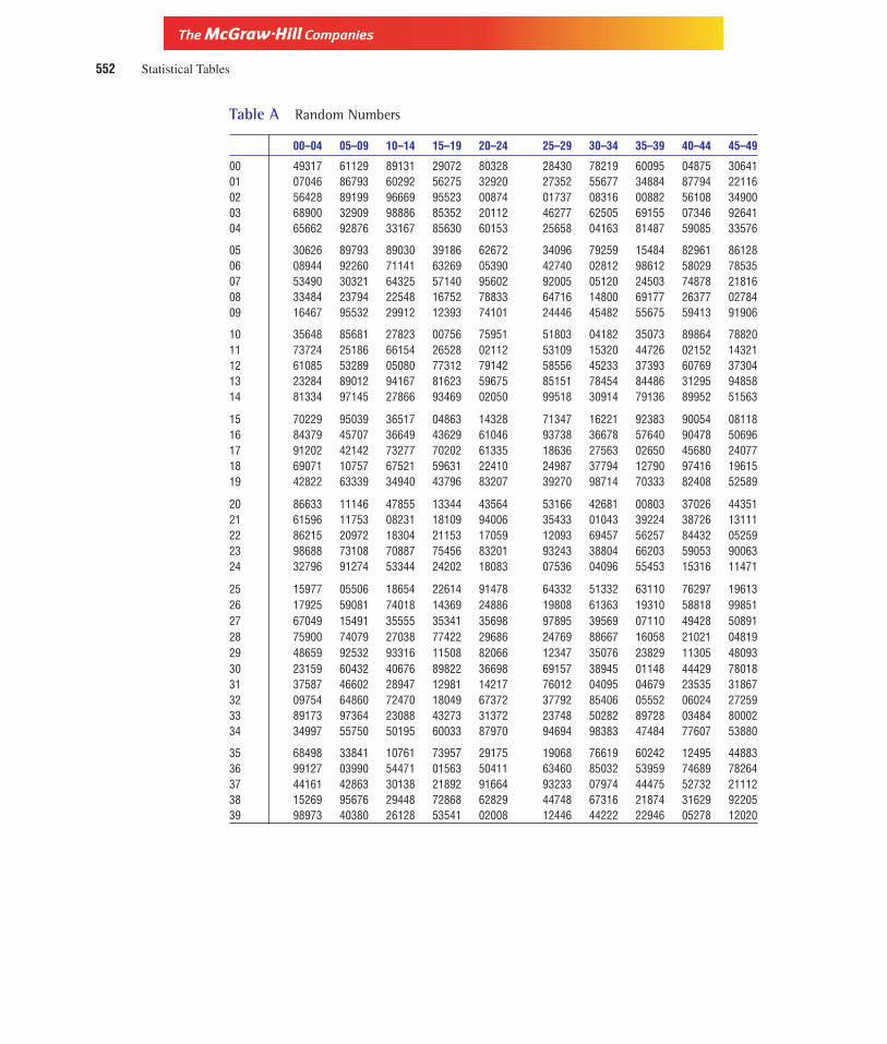
Version, Third Edition
552 Statistical Tables
Table A Random Numbers
00–04 05–09 10–14 15–19 20–24 25–29 30–34 35–39 40–44 45–49
00 49317 61129 89131 29072 80328 28430 78219 60095 04875 3064101 07046 86793 60292 56275 32920 27352 55677 34884 87794 2211602 56428 89199 96669 95523 00874 01737 08316 00882 56108 3490003 68900 32909 98886 85352 20112 46277 62505 69155 07346 9264104 65662 92876 33167 85630 60153 25658 04163 81487 59085 33576
05 30626 89793 89030 39186 62672 34096 79259 15484 82961 8612806 08944 92260 71141 63269 05390 42740 02812 98612 58029 7853507 53490 30321 64325 57140 95602 92005 05120 24503 74878 2181608 33484 23794 22548 16752 78833 64716 14800 69177 26377 0278409 16467 95532 29912 12393 74101 24446 45482 55675 59413 91906
10 35648 85681 27823 00756 75951 51803 04182 35073 89864 7882011 73724 25186 66154 26528 02112 53109 15320 44726 02152 1432112 61085 53289 05080 77312 79142 58556 45233 37393 60769 3730413 23284 89012 94167 81623 59675 85151 78454 84486 31295 9485814 81334 97145 27866 93469 02050 99518 30914 79136 89952 51563
15 70229 95039 36517 04863 14328 71347 16221 92383 90054 0811816 84379 45707 36649 43629 61046 93738 36678 57640 90478 5069617 91202 42142 73277 70202 61335 18636 27563 02650 45680 2407718 69071 10757 67521 59631 22410 24987 37794 12790 97416 1961519 42822 63339 34940 43796 83207 39270 98714 70333 82408 52589
20 86633 11146 47855 13344 43564 53166 42681 00803 37026 4435121 61596 11753 08231 18109 94006 35433 01043 39224 38726 1311122 86215 20972 18304 21153 17059 12093 69457 56257 84432 0525923 98688 73108 70887 75456 83201 93243 38804 66203 59053 9006324 32796 91274 53344 24202 18083 07536 04096 55453 15316 11471
25 15977 05506 18654 22614 91478 64332 51332 63110 76297 1961326 17925 59081 74018 14369 24886 19808 61363 19310 58818 9985127 67049 15491 35555 35341 35698 97895 39569 07110 49428 5089128 75900 74079 27038 77422 29686 24769 88667 16058 21021 0481929 48659 92532 93316 11508 82066 12347 35076 23829 11305 4809330 23159 60432 40676 89822 36698 69157 38945 01148 44429 7801831 37587 46602 28947 12981 14217 76012 04095 04679 23535 3186732 09754 64860 72470 18049 67372 37792 85406 05552 06024 2725933 89173 97364 23088 43273 31372 23748 50282 89728 03484 8000234 34997 55750 50195 60033 87970 94694 98383 47484 77607 53880
35 68498 33841 10761 73957 29175 19068 76619 60242 12495 4488336 99127 03990 54471 01563 50411 63460 85032 53959 74689 7826437 44161 42863 30138 21892 91664 93233 07974 44475 52732 2111238 15269 95676 29448 72868 62829 44748 67316 21874 31629 9220539 98973 40380 26128 53541 02008 12446 44222 22946 05278 12020

Version, Third Edition
Appendix III 553
Table A Random Numbers (continued )
50–54 55–59 60–64 65–69 70–74 75–79 80–84 85–89 90–94 95–99
00 03424 74864 11746 77342 24970 15430 76369 08232 05402 6608701 01677 84988 35246 15095 08838 31175 20982 30309 18096 8489902 57939 08859 48441 57896 84319 83283 14811 97076 89291 3591003 27552 57307 58843 38377 02136 59389 82338 26309 28637 6845204 97565 86873 98942 00360 64645 46932 71799 09485 09314 51819
05 84800 50323 33396 46177 09149 02865 00588 46994 99550 4050606 52914 13681 23381 38797 28428 48170 03086 32809 75236 0005807 54951 66790 09596 29427 05105 92584 45968 12386 07806 4065508 80362 43955 61191 47628 11426 99325 69607 28305 73922 8927109 62421 70476 37258 31697 61109 18333 91701 95563 46201 12514
10 33012 34971 29595 09899 95259 51098 16799 89517 09909 4835211 93937 10140 85341 57364 65055 85239 68144 72578 85758 2092612 47343 53008 64554 77142 54813 94272 13220 93276 12028 0584213 36728 89534 32162 58174 07438 49352 68648 65773 47769 7302614 54192 52552 94695 93188 69058 53322 86416 18973 95293 10967
15 73243 63347 17348 17122 59731 57994 34753 97620 20537 4276616 38748 95561 20099 98539 36899 30760 28145 60312 83863 9631217 95047 14426 44302 54731 18933 19080 72952 57627 56855 3485918 77174 73993 06339 33863 27247 70802 72386 35801 43204 0792319 75687 63671 09641 21688 19629 77186 34847 76911 77754 74082
20 65318 93663 57336 82518 72106 38375 45361 17294 32214 7732121 39689 65062 26294 06957 28051 32978 04044 19522 00154 0739922 86917 30252 02536 28503 08677 89051 37121 30540 24812 3325123 87081 02290 11567 64665 52242 44974 06450 82159 86458 3585724 20029 12125 22239 70058 66242 78416 53416 76656 37235 37497
25 41343 01619 68185 65843 30455 16122 43529 99837 08684 5694726 48802 86690 70360 61800 96292 54364 27178 39817 58175 6407527 00201 53674 62822 14069 80581 45643 92836 46278 82670 3751928 96157 13631 45042 85158 13973 67170 14192 72897 13882 6848729 66903 83523 64279 09547 78335 40315 74289 05578 98707 68894
30 77037 12096 69134 13504 00181 31991 79227 67942 70880 3787231 07666 49845 86053 94798 83079 50421 68467 76689 02028 5555532 60628 11373 54477 41349 96997 02999 16166 57749 13288 0535933 08193 10440 76553 44186 83076 05119 31491 82985 61346 0847334 64368 14947 82460 06619 79026 51058 65457 59765 09322 7187535 17654 34052 30839 63725 84414 76157 74516 53829 88846 77860
36 73333 12388 33682 35931 08861 84952 54744 06407 28523 2218337 71375 07499 20422 92949 04918 90317 23064 83117 82547 1758438 46163 11272 64918 50711 54539 23970 17133 55776 16550 9131339 49910 95947 81477 20980 47258 33546 64109 68526 73100 49610

Version, Third Edition
Table B Binomial Distribution
�
n X 0.05 0.10 0.15 0.20 0.25 0.30 0.35 0.40 0.45 0.50
1 0 0.9500 0.9000 0.8500 0.8000 0.7500 0.7000 0.6500 0.6000 0.5500 0.50001 0.0500 0.1000 0.1500 0.2000 0.2500 0.3000 0.3500 0.4000 0.4500 0.5000
2 0 0.9025 0.8100 0.7225 0.6400 0.5625 0.4900 0.4225 0.3600 0.3025 0.25001 0.0950 0.1800 0.2550 0.3200 0.3750 0.4200 0.4550 0.4800 0.4950 0.50002 0.0025 0.0100 0.0225 0.0400 0.0625 0.0900 0.1225 0.1600 0.2025 0.2500
3 0 0.8574 0.7290 0.6141 0.5120 0.4219 0.3430 0.2746 0.2160 0.1664 0.12501 0.1354 0.2430 0.3251 0.3840 0.4219 0.4410 0.4436 0.4320 0.4084 0.37502 0.0071 0.0270 0.0574 0.0960 0.1406 0.1890 0.2389 0.2880 0.3341 0.37503 0.0001 0.0010 0.0034 0.0080 0.0156 0.0270 0.0429 0.0640 0.0911 0.1250
4 0 0.8145 0.6561 0.5220 0.4096 0.3164 0.2401 0.1785 0.1296 0.0915 0.06251 0.1715 0.2916 0.3685 0.4096 0.4219 0.4116 0.3845 0.3456 0.2995 0.25002 0.0135 0.0486 0.0975 0.1536 0.2109 0.2646 0.3105 0.3456 0.3675 0.37503 0.0005 0.0036 0.0115 0.0256 0.0469 0.0756 0.1115 0.1536 0.2005 0.25004 0.0000 0.0001 0.0005 0.0016 0.0039 0.0081 0.0150 0.0256 0.0410 0.0625
5 0 0.7738 0.5905 0.4437 0.3277 0.2373 0.1681 0.1160 0.0778 0.0503 0.03131 0.2036 0.3281 0.3915 0.4096 0.3955 0.3602 0.3124 0.2592 0.2059 0.15632 0.0214 0.0729 0.1382 0.2048 0.2637 0.3087 0.3364 0.3456 0.3369 0.31253 0.0011 0.0081 0.0244 0.0512 0.0879 0.1323 0.1811 0.2304 0.2757 0.31254 0.0000 0.0005 0.0022 0.0064 0.0146 0.0284 0.0488 0.0768 0.1128 0.15635 0.0000 0.0000 0.0001 0.0003 0.0010 0.0024 0.0053 0.0102 0.0185 0.0313
6 0 0.7351 0.5314 0.3771 0.2621 0.1780 0.1176 0.0754 0.0467 0.0277 0.01561 0.2321 0.3543 0.3993 0.3932 0.3560 0.3025 0.2437 0.1866 0.1359 0.09382 0.0305 0.0984 0.1762 0.2458 0.2966 0.3241 0.3280 0.3110 0.2780 0.23443 0.0021 0.0146 0.0415 0.0819 0.1318 0.1852 0.2355 0.2765 0.3032 0.31254 0.0001 0.0012 0.0055 0.0154 0.0330 0.0595 0.0951 0.1382 0.1861 0.23445 0.0000 0.0001 0.0004 0.0015 0.0044 0.0102 0.0205 0.0369 0.0609 0.09386 0.0000 0.0000 0.0000 0.0001 0.0002 0.0007 0.0018 0.0041 0.0083 0.0156
7 0 0.6983 0.4783 0.3206 0.2097 0.1335 0.0824 0.0490 0.0280 0.0152 0.00781 0.2573 0.3720 0.3960 0.3670 0.3115 0.2471 0.1848 0.1306 0.0872 0.05472 0.0406 0.1240 0.2097 0.2753 0.3115 0.3177 0.2985 0.2613 0.2140 0.16413 0.0036 0.0230 0.0617 0.1147 0.1730 0.2269 0.2679 0.2903 0.2918 0.27344 0.0002 0.0026 0.0109 0.0287 0.0577 0.0972 0.1442 0.1935 0.2388 0.2734
5 0.0000 0.0002 0.0012 0.0043 0.0115 0.0250 0.0466 0.0774 0.1172 0.16416 0.0000 0.0000 0.0001 0.0004 0.0013 0.0036 0.0084 0.0172 0.0320 0.05477 0.0000 0.0000 0.0000 0.0000 0.0001 0.0002 0.0006 0.0016 0.0037 0.0078
8 0 0.6634 0.4305 0.2725 0.1678 0.1001 0.0576 0.0319 0.0168 0.0084 0.00391 0.2793 0.3826 0.3847 0.3355 0.2670 0.1977 0.1373 0.0896 0.0548 0.03132 0.0515 0.1488 0.2376 0.2936 0.3115 0.2965 0.2587 0.2090 0.1569 0.10943 0.0054 0.0331 0.0839 0.1468 0.2076 0.2541 0.2786 0.2787 0.2568 0.21884 0.0004 0.0046 0.0185 0.0459 0.0865 0.1361 0.1875 0.2322 0.2627 0.2734
5 0.0000 0.0004 0.0026 0.0092 0.0231 0.0467 0.0808 0.1239 0.1719 0.21886 0.0000 0.0000 0.0002 0.0011 0.0038 0.0100 0.0217 0.0413 0.0703 0.10947 0.0000 0.0000 0.0000 0.0001 0.0004 0.0012 0.0033 0.0079 0.0164 0.03138 0.0000 0.0000 0.0000 0.0000 0.0000 0.0001 0.0002 0.0007 0.0017 0.0039
9 0 0.6302 0.3874 0.2316 0.1342 0.0751 0.0404 0.0207 0.0101 0.0046 0.00201 0.2985 0.3874 0.3679 0.3020 0.2253 0.1556 0.1004 0.0605 0.0339 0.0176
554 Statistical Tables

Version, Third Edition
Table B Binomial Distribution (continued )
�
n X 0.05 0.10 0.15 0.20 0.25 0.30 0.35 0.40 0.45 0.50
2 0.0629 0.1722 0.2597 0.3020 0.3003 0.2668 0.2162 0.1612 0.1110 0.07033 0.0077 0.0446 0.1069 0.1762 0.2336 0.2668 0.2716 0.2508 0.2119 0.16414 0.0006 0.0074 0.0283 0.0661 0.1168 0.1715 0.2194 0.2508 0.2600 0.2461
5 0.0000 0.0008 0.0050 0.0165 0.0389 0.0735 0.1181 0.1672 0.2128 0.24616 0.0000 0.0001 0.0006 0.0028 0.0087 0.0210 0.0424 0.0743 0.1160 0.16417 0.0000 0.0000 0.0000 0.0003 0.0012 0.0039 0.0098 0.0212 0.0407 0.07038 0.0000 0.0000 0.0000 0.0000 0.0001 0.0004 0.0013 0.0035 0.0083 0.01769 0.0000 0.0000 0.0000 0.0000 0.0000 0.0000 0.0001 0.0003 0.0008 0.0020
10 0 0.5987 0.3487 0.1969 0.1074 0.0563 0.0282 0.0135 0.0060 0.0025 0.00101 0.3151 0.3874 0.3474 0.2684 0.1877 0.1211 0.0725 0.0403 0.0207 0.00982 0.0746 0.1937 0.2759 0.3020 0.2816 0.2335 0.1757 0.1209 0.0763 0.04393 0.0105 0.0574 0.1298 0.2013 0.2503 0.2668 0.2522 0.2150 0.1665 0.11724 0.0010 0.0112 0.0401 0.0881 0.1460 0.2001 0.2377 0.2508 0.2384 0.2051
5 0.0001 0.0015 0.0085 0.0264 0.0584 0.1029 0.1536 0.2007 0.2340 0.24616 0.0000 0.0001 0.0012 0.0055 0.0162 0.0368 0.0689 0.1115 0.1596 0.20517 0.0000 0.0000 0.0001 0.0008 0.0031 0.0090 0.0212 0.0425 0.0746 0.11728 0.0000 0.0000 0.0000 0.0001 0.0004 0.0014 0.0043 0.0106 0.0229 0.04399 0.0000 0.0000 0.0000 0.0000 0.0000 0.0001 0.0005 0.0016 0.0042 0.0098
10 0.0000 0.0000 0.0000 0.0000 0.0000 0.0000 0.0000 0.0001 0.0003 0.0010
11 0 0.5688 0.3138 0.1673 0.0859 0.0422 0.0198 0.0088 0.0036 0.0014 0.00051 0.3293 0.3835 0.3248 0.2362 0.1549 0.0932 0.0518 0.0266 0.0125 0.00542 0.0867 0.2131 0.2866 0.2953 0.2581 0.1998 0.1395 0.0887 0.0513 0.02693 0.0137 0.0710 0.1517 0.2215 0.2581 0.2568 0.2254 0.1774 0.1259 0.08064 0.0014 0.0158 0.0536 0.1107 0.1721 0.2201 0.2428 0.2365 0.2060 0.1611
5 0.0001 0.0025 0.0132 0.0388 0.0803 0.1321 0.1830 0.2207 0.2360 0.22566 0.0000 0.0003 0.0023 0.0097 0.0268 0.0566 0.0985 0.1471 0.1931 0.22567 0.0000 0.0000 0.0003 0.0017 0.0064 0.0173 0.0379 0.0701 0.1128 0.16118 0.0000 0.0000 0.0000 0.0002 0.0011 0.0037 0.0102 0.0234 0.0462 0.08069 0.0000 0.0000 0.0000 0.0000 0.0001 0.0005 0.0018 0.0052 0.0126 0.0269
10 0.0000 0.0000 0.0000 0.0000 0.0000 0.0000 0.0002 0.0007 0.0021 0.005411 0.0000 0.0000 0.0000 0.0000 0.0000 0.0000 0.0000 0.0000 0.0002 0.0005
12 0 0.5404 0.2824 0.1422 0.0687 0.0317 0.0138 0.0057 0.0022 0.0008 0.00021 0.3413 0.3766 0.3012 0.2062 0.1267 0.0712 0.0368 0.0174 0.0075 0.00292 0.0988 0.2301 0.2924 0.2835 0.2323 0.1678 0.1088 0.0639 0.0339 0.01613 0.0173 0.0852 0.1720 0.2362 0.2581 0.2397 0.1954 0.1419 0.0923 0.05374 0.0021 0.0213 0.0683 0.1329 0.1936 0.2311 0.2367 0.2128 0.1700 0.1208
5 0.0002 0.0038 0.0193 0.0532 0.1032 0.1585 0.2039 0.2270 0.2225 0.19346 0.0000 0.0005 0.0040 0.0155 0.0401 0.0792 0.1281 0.1766 0.2124 0.22567 0.0000 0.0000 0.0006 0.0033 0.0115 0.0291 0.0591 0.1009 0.1489 0.19348 0.0000 0.0000 0.0001 0.0005 0.0024 0.0078 0.0199 0.0420 0.0762 0.12089 0.0000 0.0000 0.0000 0.0001 0.0004 0.0015 0.0048 0.0125 0.0277 0.0537
10 0.0000 0.0000 0.0000 0.0000 0.0000 0.0002 0.0008 0.0025 0.0068 0.016111 0.0000 0.0000 0.0000 0.0000 0.0000 0.0000 0.0001 0.0003 0.0010 0.002912 0.0000 0.0000 0.0000 0.0000 0.0000 0.0000 0.0000 0.0000 0.0001 0.0002
13 0 0.5133 0.2542 0.1209 0.0550 0.0238 0.0097 0.0037 0.0013 0.0004 0.00011 0.3512 0.3672 0.2774 0.1787 0.1029 0.0540 0.0259 0.0113 0.0045 0.0016
Appendix III 555
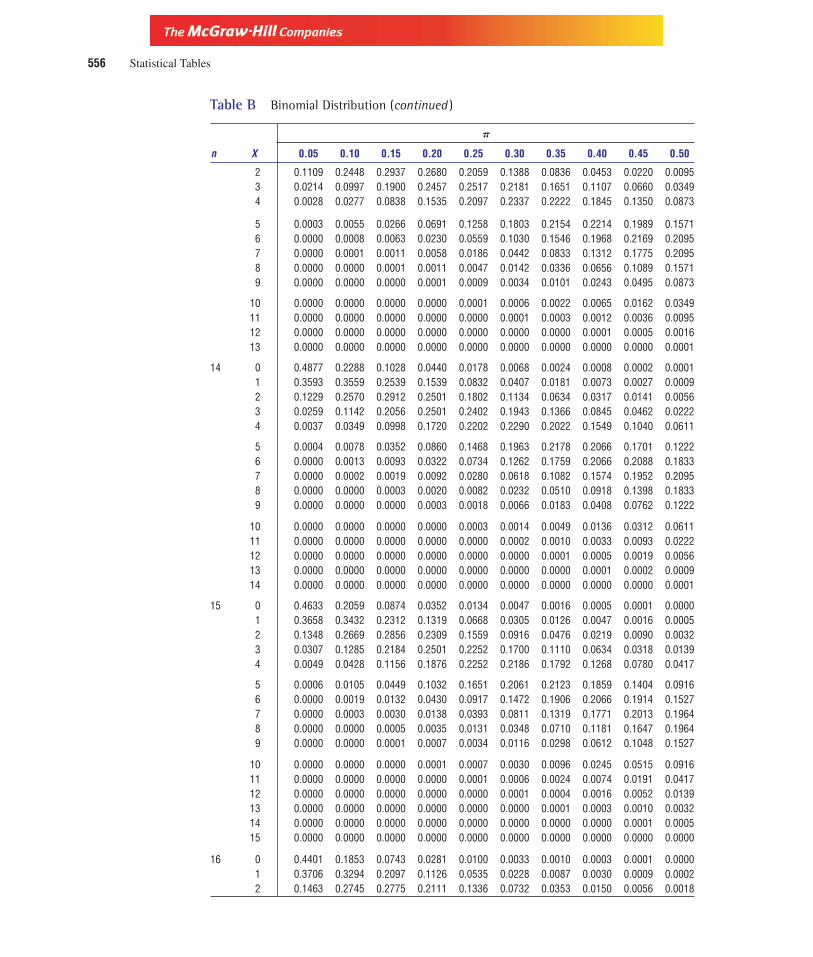
Version, Third Edition
556 Statistical Tables
Table B Binomial Distribution (continued )
�
n X 0.05 0.10 0.15 0.20 0.25 0.30 0.35 0.40 0.45 0.50
2 0.1109 0.2448 0.2937 0.2680 0.2059 0.1388 0.0836 0.0453 0.0220 0.00953 0.0214 0.0997 0.1900 0.2457 0.2517 0.2181 0.1651 0.1107 0.0660 0.03494 0.0028 0.0277 0.0838 0.1535 0.2097 0.2337 0.2222 0.1845 0.1350 0.0873
5 0.0003 0.0055 0.0266 0.0691 0.1258 0.1803 0.2154 0.2214 0.1989 0.15716 0.0000 0.0008 0.0063 0.0230 0.0559 0.1030 0.1546 0.1968 0.2169 0.20957 0.0000 0.0001 0.0011 0.0058 0.0186 0.0442 0.0833 0.1312 0.1775 0.20958 0.0000 0.0000 0.0001 0.0011 0.0047 0.0142 0.0336 0.0656 0.1089 0.15719 0.0000 0.0000 0.0000 0.0001 0.0009 0.0034 0.0101 0.0243 0.0495 0.0873
10 0.0000 0.0000 0.0000 0.0000 0.0001 0.0006 0.0022 0.0065 0.0162 0.034911 0.0000 0.0000 0.0000 0.0000 0.0000 0.0001 0.0003 0.0012 0.0036 0.009512 0.0000 0.0000 0.0000 0.0000 0.0000 0.0000 0.0000 0.0001 0.0005 0.001613 0.0000 0.0000 0.0000 0.0000 0.0000 0.0000 0.0000 0.0000 0.0000 0.0001
14 0 0.4877 0.2288 0.1028 0.0440 0.0178 0.0068 0.0024 0.0008 0.0002 0.00011 0.3593 0.3559 0.2539 0.1539 0.0832 0.0407 0.0181 0.0073 0.0027 0.00092 0.1229 0.2570 0.2912 0.2501 0.1802 0.1134 0.0634 0.0317 0.0141 0.00563 0.0259 0.1142 0.2056 0.2501 0.2402 0.1943 0.1366 0.0845 0.0462 0.02224 0.0037 0.0349 0.0998 0.1720 0.2202 0.2290 0.2022 0.1549 0.1040 0.0611
5 0.0004 0.0078 0.0352 0.0860 0.1468 0.1963 0.2178 0.2066 0.1701 0.12226 0.0000 0.0013 0.0093 0.0322 0.0734 0.1262 0.1759 0.2066 0.2088 0.18337 0.0000 0.0002 0.0019 0.0092 0.0280 0.0618 0.1082 0.1574 0.1952 0.20958 0.0000 0.0000 0.0003 0.0020 0.0082 0.0232 0.0510 0.0918 0.1398 0.18339 0.0000 0.0000 0.0000 0.0003 0.0018 0.0066 0.0183 0.0408 0.0762 0.1222
10 0.0000 0.0000 0.0000 0.0000 0.0003 0.0014 0.0049 0.0136 0.0312 0.061111 0.0000 0.0000 0.0000 0.0000 0.0000 0.0002 0.0010 0.0033 0.0093 0.022212 0.0000 0.0000 0.0000 0.0000 0.0000 0.0000 0.0001 0.0005 0.0019 0.005613 0.0000 0.0000 0.0000 0.0000 0.0000 0.0000 0.0000 0.0001 0.0002 0.000914 0.0000 0.0000 0.0000 0.0000 0.0000 0.0000 0.0000 0.0000 0.0000 0.0001
15 0 0.4633 0.2059 0.0874 0.0352 0.0134 0.0047 0.0016 0.0005 0.0001 0.00001 0.3658 0.3432 0.2312 0.1319 0.0668 0.0305 0.0126 0.0047 0.0016 0.00052 0.1348 0.2669 0.2856 0.2309 0.1559 0.0916 0.0476 0.0219 0.0090 0.00323 0.0307 0.1285 0.2184 0.2501 0.2252 0.1700 0.1110 0.0634 0.0318 0.01394 0.0049 0.0428 0.1156 0.1876 0.2252 0.2186 0.1792 0.1268 0.0780 0.0417
5 0.0006 0.0105 0.0449 0.1032 0.1651 0.2061 0.2123 0.1859 0.1404 0.09166 0.0000 0.0019 0.0132 0.0430 0.0917 0.1472 0.1906 0.2066 0.1914 0.15277 0.0000 0.0003 0.0030 0.0138 0.0393 0.0811 0.1319 0.1771 0.2013 0.19648 0.0000 0.0000 0.0005 0.0035 0.0131 0.0348 0.0710 0.1181 0.1647 0.19649 0.0000 0.0000 0.0001 0.0007 0.0034 0.0116 0.0298 0.0612 0.1048 0.1527
10 0.0000 0.0000 0.0000 0.0001 0.0007 0.0030 0.0096 0.0245 0.0515 0.091611 0.0000 0.0000 0.0000 0.0000 0.0001 0.0006 0.0024 0.0074 0.0191 0.041712 0.0000 0.0000 0.0000 0.0000 0.0000 0.0001 0.0004 0.0016 0.0052 0.013913 0.0000 0.0000 0.0000 0.0000 0.0000 0.0000 0.0001 0.0003 0.0010 0.003214 0.0000 0.0000 0.0000 0.0000 0.0000 0.0000 0.0000 0.0000 0.0001 0.000515 0.0000 0.0000 0.0000 0.0000 0.0000 0.0000 0.0000 0.0000 0.0000 0.0000
16 0 0.4401 0.1853 0.0743 0.0281 0.0100 0.0033 0.0010 0.0003 0.0001 0.00001 0.3706 0.3294 0.2097 0.1126 0.0535 0.0228 0.0087 0.0030 0.0009 0.00022 0.1463 0.2745 0.2775 0.2111 0.1336 0.0732 0.0353 0.0150 0.0056 0.0018

Version, Third Edition
Appendix III 557
Table B Binomial Distribution (continued )
�
n X 0.05 0.10 0.15 0.20 0.25 0.30 0.35 0.40 0.45 0.50
3 0.0359 0.1423 0.2285 0.2463 0.2079 0.1465 0.0888 0.0468 0.0215 0.00854 0.0061 0.0514 0.1311 0.2001 0.2252 0.2040 0.1553 0.1014 0.0572 0.0278
5 0.0008 0.0137 0.0555 0.1201 0.1802 0.2099 0.2008 0.1623 0.1123 0.06676 0.0001 0.0028 0.0180 0.0550 0.1101 0.1649 0.1982 0.1983 0.1684 0.12227 0.0000 0.0004 0.0045 0.0197 0.0524 0.1010 0.1524 0.1889 0.1969 0.17468 0.0000 0.0001 0.0009 0.0055 0.0197 0.0487 0.0923 0.1417 0.1812 0.19649 0.0000 0.0000 0.0001 0.0012 0.0058 0.0185 0.0442 0.0840 0.1318 0.1746
10 0.0000 0.0000 0.0000 0.0002 0.0014 0.0056 0.0167 0.0392 0.0755 0.122211 0.0000 0.0000 0.0000 0.0000 0.0002 0.0013 0.0049 0.0142 0.0337 0.066712 0.0000 0.0000 0.0000 0.0000 0.0000 0.0002 0.0011 0.0040 0.0115 0.027813 0.0000 0.0000 0.0000 0.0000 0.0000 0.0000 0.0002 0.0008 0.0029 0.008514 0.0000 0.0000 0.0000 0.0000 0.0000 0.0000 0.0000 0.0001 0.0005 0.0018
15 0.0000 0.0000 0.0000 0.0000 0.0000 0.0000 0.0000 0.0000 0.0001 0.000216 0.0000 0.0000 0.0000 0.0000 0.0000 0.0000 0.0000 0.0000 0.0000 0.0000
17 0 0.4181 0.1668 0.0631 0.0225 0.0075 0.0023 0.0007 0.0002 0.0000 0.00001 0.3741 0.3150 0.1893 0.0957 0.0426 0.0169 0.0060 0.0019 0.0005 0.00012 0.1575 0.2800 0.2673 0.1914 0.1136 0.0581 0.0260 0.0102 0.0035 0.00103 0.0415 0.1556 0.2359 0.2393 0.1893 0.1245 0.0701 0.0341 0.0144 0.00524 0.0076 0.0605 0.1457 0.2093 0.2209 0.1868 0.1320 0.0796 0.0411 0.0182
5 0.0010 0.0175 0.0668 0.1361 0.1914 0.2081 0.1849 0.1379 0.0875 0.04726 0.0001 0.0039 0.0236 0.0680 0.1276 0.1784 0.1991 0.1839 0.1432 0.09447 0.0000 0.0007 0.0065 0.0267 0.0668 0.1201 0.1685 0.1927 0.1841 0.14848 0.0000 0.0001 0.0014 0.0084 0.0279 0.0644 0.1134 0.1606 0.1883 0.18559 0.0000 0.0000 0.0003 0.0021 0.0093 0.0276 0.0611 0.1070 0.1540 0.1855
10 0.0000 0.0000 0.0000 0.0004 0.0025 0.0095 0.0263 0.0571 0.1008 0.148411 0.0000 0.0000 0.0000 0.0001 0.0005 0.0026 0.0090 0.0242 0.0525 0.094412 0.0000 0.0000 0.0000 0.0000 0.0001 0.0006 0.0024 0.0081 0.0215 0.047213 0.0000 0.0000 0.0000 0.0000 0.0000 0.0001 0.0005 0.0021 0.0068 0.018214 0.0000 0.0000 0.0000 0.0000 0.0000 0.0000 0.0001 0.0004 0.0016 0.0052
15 0.0000 0.0000 0.0000 0.0000 0.0000 0.0000 0.0000 0.0001 0.0003 0.001016 0.0000 0.0000 0.0000 0.0000 0.0000 0.0000 0.0000 0.0000 0.0000 0.000117 0.0000 0.0000 0.0000 0.0000 0.0000 0.0000 0.0000 0.0000 0.0000 0.0000
18 0 0.3972 0.1501 0.0536 0.0180 0.0056 0.0016 0.0004 0.0001 0.0000 0.00001 0.3763 0.3002 0.1704 0.0811 0.0338 0.0126 0.0042 0.0012 0.0003 0.00012 0.1683 0.2835 0.2556 0.1723 0.0958 0.0458 0.0190 0.0069 0.0022 0.00063 0.0473 0.1680 0.2406 0.2297 0.1704 0.1046 0.0547 0.0246 0.0095 0.00314 0.0093 0.0700 0.1592 0.2153 0.2130 0.1681 0.1104 0.0614 0.0291 0.0117
5 0.0014 0.0218 0.0787 0.1507 0.1988 0.2017 0.1664 0.1146 0.0666 0.03276 0.0002 0.0052 0.0301 0.0816 0.1436 0.1873 0.1941 0.1655 0.1181 0.07087 0.0000 0.0010 0.0091 0.0350 0.0820 0.1376 0.1792 0.1892 0.1657 0.12148 0.0000 0.0002 0.0022 0.0120 0.0376 0.0811 0.1327 0.1734 0.1864 0.16699 0.0000 0.0000 0.0004 0.0033 0.0139 0.0386 0.0794 0.1284 0.1694 0.1855
10 0.0000 0.0000 0.0001 0.0008 0.0042 0.0149 0.0385 0.0771 0.1248 0.166911 0.0000 0.0000 0.0000 0.0001 0.0010 0.0046 0.0151 0.0374 0.0742 0.121412 0.0000 0.0000 0.0000 0.0000 0.0002 0.0012 0.0047 0.0145 0.0354 0.070813 0.0000 0.0000 0.0000 0.0000 0.0000 0.0002 0.0012 0.0045 0.0134 0.0327

Version, Third Edition
Table B Binomial Distribution (continued )
�
n X 0.05 0.10 0.15 0.20 0.25 0.30 0.35 0.40 0.45 0.50
14 0.0000 0.0000 0.0000 0.0000 0.0000 0.0000 0.0002 0.0011 0.0039 0.0117
15 0.0000 0.0000 0.0000 0.0000 0.0000 0.0000 0.0000 0.0002 0.0009 0.003116 0.0000 0.0000 0.0000 0.0000 0.0000 0.0000 0.0000 0.0000 0.0001 0.000617 0.0000 0.0000 0.0000 0.0000 0.0000 0.0000 0.0000 0.0000 0.0000 0.000118 0.0000 0.0000 0.0000 0.0000 0.0000 0.0000 0.0000 0.0000 0.0000 0.0000
19 0 0.3774 0.1351 0.0456 0.0144 0.0042 0.0011 0.0003 0.0001 0.0000 0.00001 0.3774 0.2852 0.1529 0.0685 0.0268 0.0093 0.0029 0.0008 0.0002 0.00002 0.1787 0.2852 0.2428 0.1540 0.0803 0.0358 0.0138 0.0046 0.0013 0.00033 0.0533 0.1796 0.2428 0.2182 0.1517 0.0869 0.0422 0.0175 0.0062 0.00184 0.0112 0.0798 0.1714 0.2182 0.2023 0.1491 0.0909 0.0467 0.0203 0.0074
5 0.0018 0.0266 0.0907 0.1636 0.2023 0.1916 0.1468 0.0933 0.0497 0.02226 0.0002 0.0069 0.0374 0.0955 0.1574 0.1916 0.1844 0.1451 0.0949 0.05187 0.0000 0.0014 0.0122 0.0443 0.0974 0.1525 0.1844 0.1797 0.1443 0.09618 0.0000 0.0002 0.0032 0.0166 0.0487 0.0981 0.1489 0.1797 0.1771 0.14429 0.0000 0.0000 0.0007 0.0051 0.0198 0.0514 0.0980 0.1464 0.1771 0.1762
10 0.0000 0.0000 0.0001 0.0013 0.0066 0.0220 0.0528 0.0976 0.1449 0.176211 0.0000 0.0000 0.0000 0.0003 0.0018 0.0077 0.0233 0.0532 0.0970 0.144212 0.0000 0.0000 0.0000 0.0000 0.0004 0.0022 0.0083 0.0237 0.0529 0.096113 0.0000 0.0000 0.0000 0.0000 0.0001 0.0005 0.0024 0.0085 0.0233 0.051814 0.0000 0.0000 0.0000 0.0000 0.0000 0.0001 0.0006 0.0024 0.0082 0.0222
15 0.0000 0.0000 0.0000 0.0000 0.0000 0.0000 0.0001 0.0005 0.0022 0.007416 0.0000 0.0000 0.0000 0.0000 0.0000 0.0000 0.0000 0.0001 0.0005 0.001817 0.0000 0.0000 0.0000 0.0000 0.0000 0.0000 0.0000 0.0000 0.0001 0.000318 0.0000 0.0000 0.0000 0.0000 0.0000 0.0000 0.0000 0.0000 0.0000 0.000019 0.0000 0.0000 0.0000 0.0000 0.0000 0.0000 0.0000 0.0000 0.0000 0.0000
20 0 0.3585 0.1216 0.0388 0.0115 0.0032 0.0008 0.0002 0.0000 0.0000 0.00001 0.3774 0.2702 0.1368 0.0576 0.0211 0.0068 0.0020 0.0005 0.0001 0.00002 0.1887 0.2852 0.2293 0.1369 0.0669 0.0278 0.0100 0.0031 0.0008 0.00023 0.0596 0.1901 0.2428 0.2054 0.1339 0.0716 0.0323 0.0123 0.0040 0.00114 0.0133 0.0898 0.1821 0.2182 0.1897 0.1304 0.0738 0.0350 0.0139 0.0046
5 0.0022 0.0319 0.1028 0.1746 0.2023 0.1789 0.1272 0.0746 0.0365 0.01486 0.0003 0.0089 0.0454 0.1091 0.1686 0.1916 0.1712 0.1244 0.0746 0.03707 0.0000 0.0020 0.0160 0.0545 0.1124 0.1643 0.1844 0.1659 0.1221 0.07398 0.0000 0.0004 0.0046 0.0222 0.0609 0.1144 0.1614 0.1797 0.1623 0.12019 0.0000 0.0001 0.0011 0.0074 0.0271 0.0654 0.1158 0.1597 0.1771 0.1602
10 0.0000 0.0000 0.0002 0.0020 0.0099 0.0308 0.0686 0.1171 0.1593 0.176211 0.0000 0.0000 0.0000 0.0005 0.0030 0.0120 0.0336 0.0710 0.1185 0.160212 0.0000 0.0000 0.0000 0.0001 0.0008 0.0039 0.0136 0.0355 0.0727 0.120113 0.0000 0.0000 0.0000 0.0000 0.0002 0.0010 0.0045 0.0146 0.0366 0.073914 0.0000 0.0000 0.0000 0.0000 0.0000 0.0002 0.0012 0.0049 0.0150 0.0370
15 0.0000 0.0000 0.0000 0.0000 0.0000 0.0000 0.0003 0.0013 0.0049 0.014816 0.0000 0.0000 0.0000 0.0000 0.0000 0.0000 0.0000 0.0003 0.0013 0.004617 0.0000 0.0000 0.0000 0.0000 0.0000 0.0000 0.0000 0.0000 0.0002 0.001118 0.0000 0.0000 0.0000 0.0000 0.0000 0.0000 0.0000 0.0000 0.0000 0.000219 0.0000 0.0000 0.0000 0.0000 0.0000 0.0000 0.0000 0.0000 0.0000 0.0000
558 Statistical Tables

Version, Third Edition
Table C Cumulative Binomial Distribution
�
n X 0.01 0.05 0.10 0.15 0.20 0.25 0.30 0.35 0.40 0.45 0.50
2 0 0.9801 0.9025 0.8100 0.7225 0.6400 0.5625 0.4900 0.4225 0.3600 0.3025 0.25001 0.9999 0.9975 0.9900 0.9775 0.9600 0.9375 0.9100 0.8775 0.8400 0.7975 0.7500
3 0 0.9703 0.8574 0.7290 0.6141 0.5120 0.4219 0.3430 0.2746 0.2160 0.1664 0.12501 0.9997 0.9928 0.9720 0.9393 0.8960 0.8438 0.7840 0.7183 0.6480 0.5748 0.50002 1.0000 0.9999 0.9990 0.9966 0.9920 0.9844 0.9730 0.9571 0.9360 0.9089 0.8750
4 0 0.9606 0.8145 0.6561 0.5220 0.4096 0.3164 0.2401 0.1785 0.1296 0.0915 0.06251 0.9994 0.9860 0.9477 0.8905 0.8192 0.7383 0.6517 0.5630 0.4752 0.3910 0.31252 1.0000 0.9995 0.9963 0.9880 0.9728 0.9492 0.9163 0.8735 0.8208 0.7585 0.68753 1.0000 1.0000 0.9999 0.9995 0.9984 0.9961 0.9919 0.9850 0.9744 0.9590 0.9375
5 0 0.9510 0.7738 0.5905 0.4437 0.3277 0.2373 0.1681 0.1160 0.0778 0.0503 0.03131 0.9990 0.9774 0.9185 0.8352 0.7373 0.6328 0.5282 0.4284 0.3370 0.2562 0.18752 1.0000 0.9988 0.9914 0.9734 0.9421 0.8965 0.8369 0.7648 0.6826 0.5931 0.50003 1.0000 1.0000 0.9995 0.9978 0.9933 0.9844 0.9692 0.9460 0.9130 0.8688 0.81254 1.0000 1.0000 1.0000 0.9999 0.9997 0.9990 0.9976 0.9947 0.9898 0.9815 0.9688
6 0 0.9415 0.7351 0.5314 0.3771 0.2621 0.1780 0.1176 0.0754 0.0467 0.0277 0.01561 0.9985 0.9672 0.8857 0.7765 0.6554 0.5339 0.4202 0.3191 0.2333 0.1636 0.10942 1.0000 0.9978 0.9842 0.9527 0.9011 0.8306 0.7443 0.6471 0.5443 0.4415 0.34383 1.0000 0.9999 0.9987 0.9941 0.9830 0.9624 0.9295 0.8826 0.8208 0.7447 0.65634 1.0000 1.0000 0.9999 0.9996 0.9984 0.9954 0.9891 0.9777 0.9590 0.9308 0.8906
5 1.0000 1.0000 1.0000 1.0000 0.9999 0.9998 0.9993 0.9982 0.9959 0.9917 0.9844
7 0 0.9321 0.6983 0.4783 0.3206 0.2097 0.1335 0.0824 0.0490 0.0280 0.0152 0.00781 0.9980 0.9556 0.8503 0.7166 0.5767 0.4449 0.3294 0.2338 0.1586 0.1024 0.06252 1.0000 0.9962 0.9743 0.9262 0.8520 0.7564 0.6471 0.5323 0.4199 0.3164 0.22663 1.0000 0.9998 0.9973 0.9879 0.9667 0.9294 0.8740 0.8002 0.7102 0.6083 0.50004 1.0000 1.0000 0.9998 0.9988 0.9953 0.9871 0.9712 0.9444 0.9037 0.8471 0.7734
5 1.0000 1.0000 1.0000 0.9999 0.9996 0.9987 0.9962 0.9910 0.9812 0.9643 0.93756 1.0000 1.0000 1.0000 1.0000 1.0000 0.9999 0.9998 0.9994 0.9984 0.9963 0.9922
8 0 0.9227 0.6634 0.4305 0.2725 0.1678 0.1001 0.0576 0.0319 0.0168 0.0084 0.00391 0.9973 0.9428 0.8131 0.6572 0.5033 0.3671 0.2553 0.1691 0.1064 0.0632 0.03522 0.9999 0.9942 0.9619 0.8948 0.7969 0.6785 0.5518 0.4278 0.3154 0.2201 0.14453 1.0000 0.9996 0.9950 0.9786 0.9437 0.8862 0.8059 0.7064 0.5941 0.4770 0.36334 1.0000 1.0000 0.9996 0.9971 0.9896 0.9727 0.9420 0.8939 0.8263 0.7396 0.6367
5 1.0000 1.0000 1.0000 0.9998 0.9988 0.9958 0.9887 0.9747 0.9502 0.9115 0.85556 1.0000 1.0000 1.0000 1.0000 0.9999 0.9996 0.9987 0.9964 0.9915 0.9819 0.96487 1.0000 1.0000 1.0000 1.0000 1.0000 1.0000 0.9999 0.9998 0.9993 0.9983 0.9961
9 0 0.9135 0.6302 0.3874 0.2316 0.1342 0.0751 0.0404 0.0207 0.0101 0.0046 0.00201 0.9966 0.9288 0.7748 0.5995 0.4362 0.3003 0.1960 0.1211 0.0705 0.0385 0.01952 0.9999 0.9916 0.9470 0.8591 0.7382 0.6007 0.4628 0.3373 0.2318 0.1495 0.08983 1.0000 0.9944 0.9917 0.9661 0.9144 0.8343 0.7297 0.6089 0.4826 0.3614 0.25394 1.0000 1.0000 0.9991 0.9944 0.9804 0.9511 0.9012 0.8283 0.7334 0.6214 0.5000
5 1.0000 1.0000 0.9999 0.9994 0.9969 0.9900 0.9747 0.9464 0.9006 0.8342 0.74616 1.0000 1.0000 1.0000 1.0000 0.9997 0.9987 0.9957 0.9888 0.9750 0.9502 0.91027 1.0000 1.0000 1.0000 1.0000 1.0000 0.9999 0.9996 0.9986 0.9962 0.9909 0.98058 1.0000 1.0000 1.0000 1.0000 1.0000 1.0000 1.0000 0.9999 0.9997 0.9992 0.9980
10 0 0.9044 0.5987 0.3487 0.1969 0.1074 0.0563 0.0282 0.0135 0.0060 0.0025 0.0010
Appendix III 559

Version, Third Edition
Table C Cumulative Binomial Distribution (continued )
�
n X 0.01 0.05 0.10 0.15 0.20 0.25 0.30 0.35 0.40 0.45 0.50
10 1 0.9957 0.9139 0.7361 0.5443 0.3758 0.2440 0.1493 0.0860 0.0464 0.0233 0.01072 0.9999 0.9885 0.9298 0.8202 0.6778 0.5256 0.3828 0.2616 0.1673 0.0996 0.05473 1.0000 0.9990 0.9872 0.9500 0.8791 0.7759 0.6496 0.5138 0.3823 0.2660 0.17194 1.0000 0.9999 0.9984 0.9901 0.9672 0.9219 0.8497 0.7515 0.6331 0.5044 0.37705 1.0000 1.0000 0.9999 0.9986 0.9936 0.9803 0.9527 0.9051 0.8338 0.7384 0.6230
6 1.0000 1.0000 1.0000 0.9999 0.9991 0.9965 0.9894 0.9740 0.9452 0.8980 0.82817 1.0000 1.0000 1.0000 1.0000 0.9999 0.9996 0.9984 0.9952 0.9877 0.9726 0.94538 1.0000 1.0000 1.0000 1.0000 1.0000 1.0000 0.9999 0.9995 0.9983 0.9955 0.98939 1.0000 1.0000 1.0000 1.0000 1.0000 1.0000 1.0000 1.0000 0.9999 0.9997 0.9990
11 0 0.8953 0.5688 0.3138 0.1673 0.0859 0.0422 0.0198 0.0088 0.0036 0.0014 0.00051 0.9948 0.8981 0.6974 0.4922 0.3221 0.1971 0.1130 0.0606 0.0302 0.0139 0.00592 0.9998 0.9848 0.9104 0.7788 0.6174 0.4552 0.3127 0.2001 0.1189 0.0652 0.03273 1.0000 0.9984 0.9815 0.9306 0.8389 0.7133 0.5696 0.4256 0.2963 0.1911 0.11334 1.0000 0.9999 0.9972 0.9841 0.9496 0.8854 0.7897 0.6683 0.5328 0.3971 0.2744
5 1.0000 1.0000 0.9997 0.9973 0.9883 0.9657 0.9218 0.8513 0.7535 0.6331 0.50006 1.0000 1.0000 1.0000 0.9997 0.9980 0.9924 0.9784 0.9499 0.9006 0.8262 0.72567 1.0000 1.0000 1.0000 1.0000 0.9998 0.9988 0.9957 0.9878 0.9707 0.9390 0.88678 1.0000 1.0000 1.0000 1.0000 1.0000 0.9999 0.9994 0.9980 0.9941 0.9852 0.96739 1.0000 1.0000 1.0000 1.0000 1.0000 1.0000 1.0000 0.9998 0.9993 0.9978 0.9941
10 1.0000 1.0000 1.0000 1.0000 1.0000 1.0000 1.0000 1.0000 1.0000 0.9998 0.9995
12 0 0.8864 0.5404 0.2824 0.1422 0.0687 0.0317 0.0138 0.0057 0.0022 0.0008 0.00021 0.9938 0.8816 0.6590 0.4435 0.2749 0.1584 0.0850 0.0424 0.0196 0.0083 0.00322 0.9998 0.9804 0.8891 0.7358 0.5583 0.3907 0.2528 0.1513 0.0834 0.0421 0.01933 1.0000 0.9978 0.9744 0.9078 0.7946 0.6488 0.4925 0.3467 0.2253 0.1345 0.07304 1.0000 0.9998 0.9957 0.9761 0.9274 0.8424 0.7237 0.5833 0.4382 0.3044 0.1938
5 1.0000 1.0000 0.9995 0.9954 0.9806 0.9456 0.8822 0.7873 0.6652 0.5269 0.38726 1.0000 1.0000 0.9999 0.9993 0.9961 0.9857 0.9614 0.9154 0.8418 0.7393 0.61287 1.0000 1.0000 1.0000 0.9999 0.9994 0.9972 0.9905 0.9745 0.9427 0.8883 0.80628 1.0000 1.0000 1.0000 1.0000 0.9999 0.9996 0.9983 0.9944 0.9847 0.9644 0.92709 1.0000 1.0000 1.0000 1.0000 1.0000 1.0000 0.9998 0.9992 0.9972 0.9921 0.9807
10 1.0000 1.0000 1.0000 1.0000 1.0000 1.0000 1.0000 0.9999 0.9997 0.9989 0.996811 1.0000 1.0000 1.0000 1.0000 1.0000 1.0000 1.0000 1.0000 1.0000 0.9999 0.9998
13 0 0.8775 0.5133 0.2542 0.1209 0.0550 0.0238 0.0097 0.0037 0.0013 0.0004 0.00011 0.9928 0.8646 0.6213 0.3983 0.2336 0.1267 0.0637 0.0296 0.0126 0.0049 0.00172 0.9997 0.9755 0.8661 0.6920 0.5017 0.3326 0.2025 0.1132 0.0579 0.0269 0.01123 1.0000 0.9969 0.9658 0.8820 0.7473 0.5843 0.4206 0.2783 0.1686 0.0929 0.04614 1.0000 0.9997 0.9935 0.9658 0.9009 0.7940 0.6543 0.5005 0.3530 0.2279 0.1334
5 1.0000 1.0000 0.9991 0.9925 0.9700 0.9198 0.8346 0.7159 0.5744 0.4268 0.29056 1.0000 1.0000 0.9999 0.9987 0.9930 0.9757 0.9376 0.8705 0.7712 0.6437 0.50007 1.0000 1.0000 1.0000 0.9998 0.9988 0.9944 0.9818 0.9538 0.9023 0.8212 0.70958 1.0000 1.0000 1.0000 1.0000 0.9998 0.9990 0.9960 0.9874 0.9679 0.9302 0.86669 1.0000 1.0000 1.0000 1.0000 1.0000 0.9999 0.9993 0.9975 0.9922 0.9797 0.9539
10 1.0000 1.0000 1.0000 1.0000 1.0000 1.0000 0.9999 0.9997 0.9987 0.9959 0.988811 1.0000 1.0000 1.0000 1.0000 1.0000 1.0000 1.0000 1.0000 0.9999 0.9995 0.998312 1.0000 1.0000 1.0000 1.0000 1.0000 1.0000 1.0000 1.0000 1.0000 1.0000 0.9999
560 Statistical Tables

Version, Third Edition
Table C Cumulative Binomial Distribution (continued )
�
n X 0.01 0.05 0.10 0.15 0.20 0.25 0.30 0.35 0.40 0.45 0.50
14 0 0.8687 0.4877 0.2288 0.1028 0.0440 0.0178 0.0068 0.0024 0.0008 0.0002 0.00011 0.9916 0.8470 0.5846 0.3567 0.1979 0.1010 0.0475 0.0205 0.0081 0.0029 0.00092 0.9997 0.9699 0.8416 0.6479 0.4481 0.2811 0.1608 0.0839 0.0398 0.0170 0.00653 1.0000 0.9958 0.9559 0.8535 0.6982 0.5213 0.3552 0.2205 0.1243 0.0632 0.02874 1.0000 0.9996 0.9908 0.9533 0.8702 0.7415 0.5842 0.4227 0.2793 0.1672 0.0898
5 1.0000 1.0000 0.9985 0.9885 0.9561 0.8883 0.7805 0.6405 0.4859 0.3373 0.21206 1.0000 1.0000 0.9998 0.9978 0.9884 0.9617 0.9067 0.8164 0.6925 0.5461 0.39537 1.0000 1.0000 1.0000 0.9997 0.9976 0.9897 0.9685 0.9247 0.8499 0.7414 0.60478 1.0000 1.0000 1.0000 1.0000 0.9996 0.9978 0.9917 0.9757 0.9417 0.8811 0.78809 1.0000 1.0000 1.0000 1.0000 1.0000 0.9997 0.9983 0.9940 0.9825 0.9574 0.9102
10 1.0000 1.0000 1.0000 1.0000 1.0000 1.0000 0.9998 0.9989 0.9961 0.9886 0.971311 1.0000 1.0000 1.0000 1.0000 1.0000 1.0000 1.0000 0.9999 0.9994 0.9978 0.993512 1.0000 1.0000 1.0000 1.0000 1.0000 1.0000 1.0000 1.0000 0.9999 0.9997 0.999113 1.0000 1.0000 1.0000 1.0000 1.0000 1.0000 1.0000 1.0000 1.0000 1.0000 0.9999
15 0 0.8601 0.4633 0.2059 0.0874 0.0352 0.0134 0.0047 0.0016 0.0005 0.0001 0.00001 0.9904 0.8290 0.5490 0.3186 0.1671 0.0802 0.0353 0.0142 0.0052 0.0017 0.00052 0.9996 0.9638 0.8159 0.6042 0.3980 0.2361 0.1268 0.0617 0.0271 0.0107 0.00373 1.0000 0.9945 0.9444 0.8227 0.6482 0.4613 0.2969 0.1727 0.0905 0.0424 0.01764 1.0000 0.9994 0.9873 0.9383 0.8358 0.6865 0.5155 0.3519 0.2173 0.1204 0.0592
5 1.0000 0.9999 0.9978 0.9832 0.9389 0.8516 0.7216 0.5643 0.4032 0.2608 0.15096 1.0000 1.0000 0.9997 0.9964 0.9819 0.9434 0.8689 0.7548 0.6098 0.4522 0.30367 1.0000 1.0000 1.0000 0.9994 0.9958 0.9827 0.9500 0.8868 0.7869 0.6535 0.50008 1.0000 1.0000 1.0000 0.9999 0.9992 0.9958 0.9848 0.9578 0.9050 0.8182 0.69649 1.0000 1.0000 1.0000 1.0000 0.9999 0.9992 0.9963 0.9876 0.9662 0.9231 0.8491
10 1.0000 1.0000 1.0000 1.0000 1.0000 0.9999 0.9993 0.9972 0.9907 0.9745 0.940811 1.0000 1.0000 1.0000 1.0000 1.0000 1.0000 0.9999 0.9995 0.9981 0.9937 0.982412 1.0000 1.0000 1.0000 1.0000 1.0000 1.0000 1.0000 0.9999 0.9997 0.9989 0.996313 1.0000 1.0000 1.0000 1.0000 1.0000 1.0000 1.0000 1.0000 1.0000 0.9999 0.999514 1.0000 1.0000 1.0000 1.0000 1.0000 1.0000 1.0000 1.0000 1.0000 1.0000 1.0000
16 0 0.8515 0.4401 0.1853 0.0743 0.0281 0.0100 0.0033 0.0010 0.0003 0.0001 0.00001 0.9891 0.8108 0.5147 0.2839 0.1407 0.0635 0.0261 0.0098 0.0033 0.0010 0.00032 0.9995 0.9571 0.7892 0.5614 0.3518 0.1971 0.0994 0.0451 0.0183 0.0066 0.00213 1.0000 0.9930 0.9316 0.7899 0.5981 0.4050 0.2459 0.1339 0.0651 0.0281 0.01064 1.0000 0.9991 0.9830 0.9209 0.7982 0.6302 0.4499 0.2892 0.1666 0.0853 0.0384
5 1.0000 0.9999 0.9967 0.9765 0.9183 0.8103 0.6598 0.4900 0.3288 0.1976 0.10516 1.0000 1.0000 0.9995 0.9944 0.9733 0.9204 0.8247 0.6881 0.5272 0.3660 0.22727 1.0000 1.0000 0.9999 0.9989 0.9930 0.9729 0.9256 0.8406 0.7161 0.5629 0.40188 1.0000 1.0000 1.0000 0.9998 0.9985 0.9925 0.9743 0.9329 0.8577 0.7441 0.59829 1.0000 1.0000 1.0000 1.0000 0.9998 0.9984 0.9929 0.9771 0.9417 0.8759 0.7728
10 1.0000 1.0000 1.0000 1.0000 1.0000 0.9997 0.9984 0.9938 0.9809 0.9514 0.894911 1.0000 1.0000 1.0000 1.0000 1.0000 1.0000 0.9997 0.9987 0.9951 0.9851 0961612 1.0000 1.0000 1.0000 1.0000 1.0000 1.0000 1.0000 0.9998 0.9991 0.9965 0.989413 1.0000 1.0000 1.0000 1.0000 1.0000 1.0000 1.0000 1.0000 0.9999 0.9994 0.997914 1.0000 1.0000 1.0000 1.0000 1.0000 1.0000 1.0000 1.0000 1.0000 0.9999 0.9997
15 1.0000 1.0000 1.0000 1.0000 1.0000 1.0000 1.0000 1.0000 1.0000 1.0000 1.0000
Appendix III 561

Version, Third Edition
Table C Cumulative Binomial Distribution (continued )
�
n X 0.01 0.05 0.10 0.15 0.20 0.25 0.30 0.35 0.40 0.45 0.50
17 0 0.8429 0.4181 0.1668 0.0631 0.0225 0.0075 0.0023 0.0007 0.0002 0.0000 0.00001 0.9877 0.7922 0.4818 0.2525 0.1182 0.0501 0.0193 0.0067 0.0021 0.0006 0.00012 0.9994 0.9497 0.7618 0.5198 0.3096 0.1637 0.0774 0.0327 0.0123 0.0041 0.00123 1.0000 0.9912 0.9174 0.7556 0.5489 0.3530 0.2019 0.1028 0.0464 0.0184 0.00644 1.0000 0.9988 0.9779 0.9013 0.7582 0.5739 0.3887 0.2348 0.1260 0.0596 0.0245
5 1.0000 0.9999 0.9953 0.9681 0.8943 0.7653 0.5968 0.4197 0.2639 0.1471 0.07176 1.0000 1.0000 0.9992 0.9917 0.9623 0.8929 0.7752 0.6188 0.4478 0.2902 0.16627 1.0000 1.0000 0.9999 0.9983 0.9891 0.9598 0.8954 0.7872 0.6405 0.4743 0.31458 1.0000 1.0000 1.0000 0.9997 0.9974 0.9876 0.9597 0.9006 0.8011 0.6626 0.50009 1.0000 1.0000 1.0000 1.0000 0.9995 0.9969 0.9873 0.9617 0.9081 0.8166 0.6855
10 1.0000 1.0000 1.0000 1.0000 0.9999 0.9994 0.9968 0.9880 0.9652 0.9174 0.833811 1.0000 1.0000 1.0000 1.0000 1.0000 0.9999 0.9993 0.9970 0.9894 0.9699 0.928312 1.0000 1.0000 1.0000 1.0000 1.0000 1.0000 0.9999 0.9994 0.9975 0.9914 0.975513 1.0000 1.0000 1.0000 1.0000 1.0000 1.0000 1.0000 0.9999 0.9995 0.9981 0.993614 1.0000 1.0000 1.0000 1.0000 1.0000 1.0000 1.0000 1.0000 0.9999 0.9997 0.9988
15 1.0000 1.0000 1.0000 1.0000 1.0000 1.0000 1.0000 1.0000 1.0000 1.0000 0.999916 1.0000 1.0000 1.0000 1.0000 1.0000 1.0000 1.0000 1.0000 1.0000 1.0000 1.0000
18 0 0.8345 0.3972 0.1501 0.0536 0.0180 0.0056 0.0016 0.0004 0.0001 0.0000 0.00001 0.9862 0.7735 0.4503 0.2241 0.0991 0.0395 0.0142 0.0046 0.0013 0.0003 0.00012 0.9993 0.9419 0.7338 0.4797 0.2713 0.1353 0.0600 0.0236 0.0082 0.0025 0.00073 1.0000 0.9891 0.9018 0.7202 0.5010 0.3057 0.1646 0.0783 0.0328 0.0120 0.00384 1.0000 0.9985 0.9718 0.8794 0.7164 0.5187 0.3327 0.1886 0.0942 0.0411 0.0154
5 1.0000 0.9998 0.9936 0.9581 0.8671 0.7175 0.5344 0.3550 0.2088 0.1077 0.04816 1.0000 1.0000 0.9988 0.9882 0.9487 0.8610 0.7217 0.5491 0.3743 0.2258 0.11897 1.0000 1.0000 0.9998 0.9973 0.9837 0.9431 0.8593 0.7283 0.5634 0.3915 0.24038 1.0000 1.0000 1.0000 0.9995 0.9957 0.9807 0.9404 0.8609 0.7368 0.5778 0.40739 1.0000 1.0000 1.0000 0.9999 0.9991 0.9946 0.9790 0.9403 0.8653 0.7473 0.5927
10 1.0000 1.0000 1.0000 1.0000 0.9998 0.9988 0.9939 0.9788 0.9424 0.8720 0.759711 1.0000 1.0000 1.0000 1.0000 1.0000 0.9998 0.9986 0.9938 0.9797 0.9463 0.881112 1.0000 1.0000 1.0000 1.0000 1.0000 1.0000 0.9997 0.9986 0.9942 0.9817 0.951913 1.0000 1.0000 1.0000 1.0000 1.0000 1.0000 1.0000 0.9997 0.9987 0.9951 0.984614 1.0000 1.0000 1.0000 1.0000 1.0000 1.0000 1.0000 1.0000 0.9998 0.9990 0.9962
15 1.0000 1.0000 1.0000 1.0000 1.0000 1.0000 1.0000 1.0000 1.0000 0.9999 0.999316 1.0000 1.0000 1.0000 1.0000 1.0000 1.0000 1.0000 1.0000 1.0000 1.0000 0.999917 1.0000 1.0000 1.0000 1.0000 1.0000 1.0000 1.0000 1.0000 1.0000 1.0000 1.0000
19 0 0.8262 0.3774 0.1351 0.0456 0.0144 0.0042 0.0011 0.0003 0.0001 0.0000 0.00001 0.9847 0.7547 0.4203 0.1985 0.0829 0.0310 0.0104 0.0031 0.0008 0.0002 0.00002 0.9991 0.9335 0.7054 0.4413 0.2369 0.1113 0.0462 0.0170 0.0055 0.0015 0.00043 1.0000 0.9868 0.8850 0.6841 0.4551 0.2631 0.1332 0.0591 0.0230 0.0077 0.00224 1.0000 0.9980 0.9648 0.8556 0.6733 0.4654 0.2822 0.1500 0.0696 0.0280 0.0096
5 1.0000 0.9998 0.9914 0.9463 0.8369 0.6678 0.4739 0.2968 0.1629 0.0777 0.03186 1.0000 1.0000 0.9983 0.9837 0.9324 0.8251 0.6655 0.4812 0.3081 0.1727 0.08357 1.0000 1.0000 0.9997 0.9959 0.9767 0.9225 0.8180 0.6656 0.4878 0.3169 0.17968 1.0000 1.0000 1.0000 0.9992 0.9933 0.9713 0.9161 0.8145 0.6675 0.4940 0.32389 1.0000 1.0000 1.0000 0.9999 0.9984 0.9911 0.9674 0.9125 0.8139 0.6710 0.5000
562 Statistical Tables

Version, Third Edition
Table C Cumulative Binomial Distribution (continued )
�
n X 0.01 0.05 0.10 0.15 0.20 0.25 0.30 0.35 0.40 0.45 0.50
10 1.0000 1.0000 1.0000 1.0000 0.9997 0.9977 0.9895 0.9653 0.9115 0.8159 0.676211 1.0000 1.0000 1.0000 1.0000 1.0000 0.9995 0.9972 0.9886 0.9648 0.9129 0.820412 1.0000 1.0000 1.0000 1.0000 1.0000 0.9999 0.9994 0.9969 0.9884 0.9658 0.916513 1.0000 1.0000 1.0000 1.0000 1.0000 1.0000 0.9999 0.9993 0.9969 0.9891 0.968214 1.0000 1.0000 1.0000 1.0000 1.0000 1.0000 1.0000 0.9999 0.9994 0.9972 0.9904
15 1.0000 1.0000 1.0000 1.0000 1.0000 1.0000 1.0000 1.0000 0.9999 0.9995 0.997816 1.0000 1.0000 1.0000 1.0000 1.0000 1.0000 1.0000 1.0000 1.0000 0.9999 0.999617 1.0000 1.0000 1.0000 1.0000 1.0000 1.0000 1.0000 1.0000 1.0000 1.0000 1.0000
20 0 0.8179 0.3585 0.1216 0.0388 0.0115 0.0032 0.0008 0.0002 0.0000 0.0000 0.00001 0.9831 0.7358 0.3917 0.1756 0.0692 0.0243 0.0076 0.0021 0.0005 0.0001 0.00002 0.9990 0.9245 0.6769 0.4049 0.2061 0.0913 0.0355 0.0121 0.0036 0.0009 0.00023 1.0000 0.9841 0.8670 0.6477 0.4114 0.2252 0.1071 0.0444 0.0160 0.0049 0.00134 1.0000 0.9974 0.9568 0.8298 0.6296 0.4148 0.2375 0.1182 0.0510 0.0189 0.0059
5 1.0000 0.9997 0.9887 0.9327 0.8042 0.6172 0.4164 0.2454 0.1256 0.0553 0.02076 1.0000 1.0000 0.9976 0.9781 0.9133 0.7858 0.6080 0.4166 0.2500 0.1299 0.05777 1.0000 1.0000 0.9996 0.9941 0.9679 0.8982 0.7723 0.6010 0.4159 0.2520 0.13168 1.0000 1.0000 0.9999 0.9987 0.9900 0.9591 0.8867 0.7624 0.5956 0.4143 0.25179 1.0000 1.0000 1.0000 0.9998 0.9974 0.9861 0.9520 0.8782 0.7553 0.5914 0.4119
10 1.0000 1.0000 1.0000 1.0000 0.9994 0.9961 0.9829 0.9468 0.8725 0.7507 0.588111 1.0000 1.0000 1.0000 1.0000 0.9999 0.9991 0.9949 0.9804 0.9435 0.8692 0.748312 1.0000 1.0000 1.0000 1.0000 1.0000 0.9998 0.9987 0.9940 0.9790 0.9420 0.868413 1.0000 1.0000 1.0000 1.0000 1.0000 1.0000 0.9997 0.9985 0.9935 0.9786 0.942314 1.0000 1.0000 1.0000 1.0000 1.0000 1.0000 1.0000 0.9997 0.9984 0.9936 0.9793
15 1.0000 1.0000 1.0000 1.0000 1.0000 1.0000 1.0000 1.0000 0.9997 0.9985 0.994116 1.0000 1.0000 1.0000 1.0000 1.0000 1.0000 1.0000 1.0000 1.0000 0.9997 0.998717 1.0000 1.0000 1.0000 1.0000 1.0000 1.0000 1.0000 1.0000 1.0000 1.0000 0.999818 1.0000 1.0000 1.0000 1.0000 1.0000 1.0000 1.0000 1.0000 1.0000 1.0000 1.0000
21 0 0.8097 0.3406 0.1094 0.0329 0.0092 0.0024 0.0006 0.0001 0.0000 0.0000 0.00001 0.9815 0.7170 0.3647 0.1550 0.0576 0.0190 0.0056 0.0014 0.0003 0.0001 0.00002 0.9988 0.9151 0.6484 0.3705 0.1787 0.0745 0.0271 0.0086 0.0024 0.0006 0.00013 0.9999 0.9811 0.8480 0.6113 0.3704 0.1917 0.0856 0.0331 0.0110 0.0031 0.00074 1.0000 0.9968 0.9478 0.8025 0.5860 0.3674 0.1984 0.0924 0.0370 0.0126 0.0036
5 1.0000 0.9996 0.9856 0.9173 0.7693 0.5666 0.3627 0.2009 0.0957 0.0389 0.01336 1.0000 1.0000 0.9967 0.9713 0.8915 0.7436 0.5505 0.3567 0.2002 0.0964 0.03927 1.0000 1.0000 0.9994 0.9917 0.9569 0.8701 0.7230 0.5365 0.3495 0.1971 0.09468 1.0000 1.0000 0.9999 0.9980 0.9856 0.9439 0.8523 0.7059 0.5237 0.3413 0.19179 1.0000 1.0000 1.0000 0.9996 0.9959 0.9794 0.9324 0.8377 0.6914 0.5117 0.3318
10 1.0000 1.0000 1.0000 0.9999 0.9990 0.9936 0.9736 0.9228 0.8256 0.6790 0.500011 1.0000 1.0000 1.0000 1.0000 0.9998 0.9983 0.9913 0.9687 0.9151 0.8159 0.668212 1.0000 1.0000 1.0000 1.0000 1.0000 0.9996 0.9976 0.9892 0.9648 0.9092 0.808313 1.0000 1.0000 1.0000 1.0000 1.0000 0.9999 0.9994 0.9969 0.9877 0.9621 0.905414 1.0000 1.0000 1.0000 1.0000 1.0000 1.0000 0.9999 0.9993 0.9964 0.9868 0.9608
15 1.0000 1.0000 1.0000 1.0000 1.0000 1.0000 1.0000 0.9999 0.9992 0.9963 0.986716 1.0000 1.0000 1.0000 1.0000 1.0000 1.0000 1.0000 1.0000 0.9998 0.9992 0.996417 1.0000 1.0000 1.0000 1.0000 1.0000 1.0000 1.0000 1.0000 1.0000 0.9999 0.9993
Appendix III 563

Version, Third Edition
Table C Cumulative Binomial Distribution (continued )
�
n X 0.01 0.05 0.10 0.15 0.20 0.25 0.30 0.35 0.40 0.45 0.50
18 1.0000 1.0000 1.0000 1.0000 1.0000 1.0000 1.0000 1.0000 1.0000 1.0000 0.999919 1.0000 1.0000 1.0000 1.0000 1.0000 1.0000 1.0000 1.0000 1.0000 1.0000 1.0000
22 0 0.8016 0.3235 0.0985 0.0280 0.0074 0.0018 0.0004 0.0001 0.0000 0.0000 0.00001 0.9798 0.6982 0.3392 0.1367 0.0480 0.0149 0.0041 0.0010 0.0002 0.0000 0.00002 0.9987 0.9052 0.6200 0.3382 0.1545 0.0606 0.0207 0.0061 0.0016 0.0003 0.00013 0.9999 0.9778 0.8281 0.5752 0.3320 0.1624 0.0681 0.0245 0.0076 0.0020 0.00044 1.0000 0.9960 0.9379 0.7738 0.5429 0.3235 0.1645 0.0716 0.0266 0.0083 0.0022
5 1.0000 0.9994 0.9818 0.9001 0.7326 0.5168 0.3134 0.1629 0.0722 0.0271 0.00856 1.0000 0.9999 0.9956 0.9632 0.8670 0.6994 0.4942 0.3022 0.1584 0.0705 0.02627 1.0000 1.0000 0.9991 0.9886 0.9439 0.8385 0.6713 0.4736 0.2898 0.1518 0.06698 1.0000 1.0000 0.9999 0.9970 0.9799 0.9254 0.8135 0.6466 0.4540 0.2764 0.14319 1.0000 1.0000 1.0000 0.9993 0.9939 0.9705 0.9084 0.7916 0.6244 0.4350 0.2617
10 1.0000 1.0000 1.0000 0.9999 0.9984 0.9900 0.9613 0.8930 0.7720 0.6037 0.415911 1.0000 1.0000 1.0000 1.0000 0.9997 0.9971 0.9860 0.9526 0.8793 0.7543 0.584112 1.0000 1.0000 1.0000 1.0000 0.9999 0.9993 0.9957 0.9820 0.9449 0.8672 0.738313 1.0000 1.0000 1.0000 1.0000 1.0000 0.9999 0.9989 0.9942 0.9785 0.9383 0.856914 1.0000 1.0000 1.0000 1.0000 1.0000 1.0000 0.9998 0.9984 0.9930 0.9757 0.9331
15 1.0000 1.0000 1.0000 1.0000 1.0000 1.0000 1.0000 0.9997 0.9981 0.9920 0.973816 1.0000 1.0000 1.0000 1.0000 1.0000 1.0000 1.0000 0.9999 0.9996 0.9979 0.991517 1.0000 1.0000 1.0000 1.0000 1.0000 1.0000 1.0000 1.0000 0.9999 0.9995 0.997818 1.0000 1.0000 1.0000 1.0000 1.0000 1.0000 1.0000 1.0000 1.0000 0.9999 0.999619 1.0000 1.0000 1.0000 1.0000 1.0000 1.0000 1.0000 1.0000 1.0000 1.0000 0.9999
20 1.0000 1.0000 1.0000 1.0000 1.0000 1.0000 1.0000 1.0000 1.0000 1.0000 1.0000
23 0 0.7936 0.3074 0.0886 0.0238 0.0059 0.0013 0.0003 0.0000 0.0000 0.0000 0.00001 0.9780 0.6794 0.3151 0.1204 0.0398 0.0116 0.0030 0.0007 0.0001 0.0000 0.00002 0.9985 0.8948 0.5920 0.3080 0.1332 0.0492 0.0157 0.0043 0.0010 0.0002 0.00003 0.9999 0.9742 0.8073 0.5396 0.2965 0.1370 0.0538 0.0181 0.0052 0.0012 0.00024 1.0000 0.9951 0.9269 0.7440 0.5007 0.2832 0.1356 0.0551 0.0190 0.0055 0.0013
5 1.0000 0.9992 0.9774 0.8811 0.6947 0.4685 0.2688 0.1309 0.0540 0.0186 0.00536 1.0000 0.9999 0.9942 0.9537 0.8402 0.6537 0.4399 0.2534 0.1240 0.0510 0.01737 1.0000 1.0000 0.9988 0.9848 0.9285 0.8037 0.6181 0.4136 0.2373 0.1152 0.04668 1.0000 1.0000 0.9998 0.9958 0.9727 0.9037 0.7709 0.5860 0.3884 0.2203 0.10509 1.0000 1.0000 1.0000 0.9990 0.9911 0.9592 0.8799 0.7408 0.5562 0.3636 0.2024
10 1.0000 1.0000 1.0000 0.9998 0.9975 0.9851 0.9454 0.8575 0.7129 0.5278 0.338811 1.0000 1.0000 1.0000 1.0000 0.9994 0.9954 0.9786 0.9318 0.8364 0.6865 0.500012 1.0000 1.0000 1.0000 1.0000 0.9999 0.9988 0.9928 0.9717 0.9187 0.8164 0.661213 1.0000 1.0000 1.0000 1.0000 1.0000 0.9997 0.9979 0.9900 0.9651 0.9063 0.797614 1.0000 1.0000 1.0000 1.0000 1.0000 0.9999 0.9995 0.9970 0.9872 0.9589 0.8950
15 1.0000 1.0000 1.0000 1.0000 1.0000 1.0000 0.9999 0.9992 0.9960 0.9847 0.953416 1.0000 1.0000 1.0000 1.0000 1.0000 1.0000 1.0000 0.9998 0.9990 0.9952 0.982717 1.0000 1.0000 1.0000 1.0000 1.0000 1.0000 1.0000 1.0000 0.9998 0.9988 0.994718 1.0000 1.0000 1.0000 1.0000 1.0000 1.0000 1.0000 1.0000 1.0000 0.9998 0.998719 1.0000 1.0000 1.0000 1.0000 1.0000 1.0000 1.0000 1.0000 1.0000 1.0000 0.9998
20 1.0000 1.0000 1.0000 1.0000 1.0000 1.0000 1.0000 1.0000 1.0000 1.0000 1.0000
564 Statistical Tables

Version, Third Edition
Table C Cumulative Binomial Distribution (continued )
�
n X 0.01 0.05 0.10 0.15 0.20 0.25 0.30 0.35 0.40 0.45 0.50
24 0 0.7857 0.2920 0.0798 0.0202 0.0047 0.0010 0.0002 0.0000 0.0000 0.0000 0.00001 0.9761 0.6608 0.2925 0.1059 0.0331 0.0090 0.0022 0.0005 0.0001 0.0000 0.00002 0.9983 0.8841 0.5643 0.2798 0.1145 0.0398 0.0119 0.0030 0.0007 0.0001 0.00003 0.9999 0.9702 0.7857 0.5049 0.2639 0.1150 0.0424 0.0133 0.0035 0.0008 0.00014 1.0000 0.9940 0.9149 0.7134 0.4599 0.2466 0.1111 0.0422 0.0134 0.0036 0.0008
5 1.0000 0.9990 0.9723 0.8606 0.6559 0.4222 0.2288 0.1044 0.0400 0.0127 0.00336 1.0000 0.9999 0.9925 0.9428 0.8111 0.6074 0.3886 0.2106 0.0960 0.0364 0.01137 1.0000 1.0000 0.9983 0.9801 0.9108 0.7662 0.5647 0.3575 0.1919 0.0863 0.03208 1.0000 1.0000 0.9997 0.9941 0.9638 0.8787 0.7250 0.5257 0.3279 0.1730 0.07589 1.0000 1.0000 0.9999 0.9985 0.9874 0.9453 0.8472 0.6866 0.4891 0.2991 0.1537
10 1.0000 1.0000 1.0000 0.9997 0.9962 0.9787 0.9258 0.8167 0.6502 0.4539 0.270611 1.0000 1.0000 1.0000 0.9999 0.9990 0.9928 0.9686 0.9058 0.7870 0.6151 0.419412 1.0000 1.0000 1.0000 1.0000 0.9998 0.9979 0.9885 0.9577 0.8857 0.7580 0.580613 1.0000 1.0000 1.0000 1.0000 1.0000 0.9995 0.9964 0.9836 0.9465 0.8659 0.729414 1.0000 1.0000 1.0000 1.0000 1.0000 0.9999 0.9990 0.9945 0.9783 0.9352 0.8463
15 1.0000 1.0000 1.0000 1.0000 1.0000 1.0000 0.9998 0.9984 0.9925 0.9731 0.924216 1.0000 1.0000 1.0000 1.0000 1.0000 1.0000 1.0000 0.9996 0.9978 0.9905 0.968017 1.0000 1.0000 1.0000 1.0000 1.0000 1.0000 1.0000 0.9999 0.9995 0.9972 0.988718 1.0000 1.0000 1.0000 1.0000 1.0000 1.0000 1.0000 1.0000 0.9999 0.9993 0.996719 1.0000 1.0000 1.0000 1.0000 1.0000 1.0000 1.0000 1.0000 1.0000 0.9999 0.9992
20 1.0000 1.0000 1.0000 1.0000 1.0000 1.0000 1.0000 1.0000 1.0000 1.0000 0.999921 1.0000 1.0000 1.0000 1.0000 1.0000 1.0000 1.0000 1.0000 1.0000 1.0000 1.0000
25 0 0.7778 0.2774 0.0718 0.0172 0.0038 0.0008 0.0001 0.0000 0.0000 0.0000 0.00001 0.9742 0.6424 0.2712 0.0931 0.0274 0.0070 0.0016 0.0003 0.0001 0.0000 0.00002 0.9980 0.8729 0.5371 0.2537 0.0982 0.0321 0.0090 0.0021 0.0004 0.0001 0.00003 0.9999 0.9659 0.7636 0.4711 0.2340 0.0962 0.0332 0.0097 0.0024 0.0005 0.00014 1.0000 0.9928 0.9020 0.6821 0.4207 0.2137 0.0905 0.0320 0.0095 0.0023 0.0005
5 1.0000 0.9988 0.9666 0.8385 0.6167 0.3783 0.1935 0.0826 0.0294 0.0086 0.00206 1.0000 0.9998 0.9905 0.9305 0.7800 0.5611 0.3407 0.1734 0.0736 0.0258 0.00737 1.0000 1.0000 0.9977 0.9745 0.8909 0.7265 0.5118 0.3061 0.1536 0.0639 0.02168 1.0000 1.0000 0.9995 0.9920 0.9532 0.8506 0.6769 0.4668 0.2735 0.1340 0.05399 1.0000 1.0000 0.9999 0.9979 0.9827 0.9287 0.8106 0.6303 0.4246 0.2424 0.1148
10 1.0000 1.0000 1.0000 0.9995 0.9944 0.9703 0.9022 0.7712 0.5858 0.3843 0.212211 1.0000 1.0000 1.0000 0.9999 0.9985 0.9893 0.9558 0.8746 0.7323 0.5426 0.345012 1.0000 1.0000 1.0000 1.0000 0.9996 0.9966 0.9825 0.9396 0.8462 0.6937 0.500013 1.0000 1.0000 1.0000 1.0000 0.9999 0.9991 0.9940 0.9745 0.9222 0.8173 0.655014 1.0000 1.0000 1.0000 1.0000 1.0000 0.9998 0.9982 0.9907 0.9656 0.9040 0.7878
15 1.0000 1.0000 1.0000 1.0000 1.0000 1.0000 0.9995 0.9971 0.9868 0.9560 0.885216 1.0000 1.0000 1.0000 1.0000 1.0000 1.0000 0.9999 0.9992 0.9957 0.9826 0.946117 1.0000 1.0000 1.0000 1.0000 1.0000 1.0000 1.0000 0.9998 0.9988 0.9942 0.978418 1.0000 1.0000 1.0000 1.0000 1.0000 1.0000 1.0000 1.0000 0.9997 0.9984 0.992719 1.0000 1.0000 1.0000 1.0000 1.0000 1.0000 1.0000 1.0000 0.9999 0.9996 0.9980
20 1.0000 1.0000 1.0000 1.0000 1.0000 1.0000 1.0000 1.0000 1.0000 0.9999 0.999521 1.0000 1.0000 1.0000 1.0000 1.0000 1.0000 1.0000 1.0000 1.0000 1.0000 0.999922 1.0000 1.0000 1.0000 1.0000 1.0000 1.0000 1.0000 1.0000 1.0000 1.0000 1.0000
Appendix III 565

Version, Third Edition
Table C Cumulative Binomial Distribution (continued )
�
n X 0.01 0.05 0.10 0.15 0.20 0.25 0.30 0.35 0.40 0.45 0.50
50 0 0.6050 0.0769 0.0052 0.0003 0.0000 0.0000 0.0000 0.0000 0.0000 0.0000 0.00001 0.9106 0.2794 0.0338 0.0029 0.0002 0.0000 0.0000 0.0000 0.0000 0.0000 0.00002 0.9862 0.5405 0.1117 0.0142 0.0013 0.0001 0.0000 0.0000 0.0000 0.0000 0.00003 0.9984 0.7604 0.2503 0.0460 0.0057 0.0005 0.0000 0.0000 0.0000 0.0000 0.00004 0.9999 0.8964 0.4312 0.1121 0.0185 0.0021 0.0002 0.0000 0.0000 0.0000 0.0000
5 1.0000 0.9622 0.6161 0.2194 0.0480 0.0070 0.0007 0.0001 0.0000 0.0000 0.00006 1.0000 0.9882 0.7702 0.3613 0.1034 0.0194 0.0025 0.0002 0.0000 0.0000 0.00007 1.0000 0.9968 0.8779 0.5188 0.1904 0.0453 0.0073 0.0008 0.0001 0.0000 0.00008 1.0000 0.9992 0.9421 0.6681 0.3073 0.0916 0.0183 0.0025 0.0002 0.0000 0.00009 1.0000 0.9998 0.9755 0.7911 0.4437 0.1637 0.0402 0.0067 0.0008 0.0001 0.0000
10 1.0000 1.0000 0.9906 0.8801 0.5836 0.2622 0.0789 0.0160 0.0022 0.0002 0.000011 1.0000 1.0000 0.9968 0.9372 0.7107 0.3816 0.1390 0.0342 0.0057 0.0006 0.000012 1.0000 1.0000 0.9990 0.9699 0.8139 0.5110 0.2229 0.0661 0.0133 0.0018 0.000213 1.0000 1.0000 0.9997 0.9868 0.8894 0.6370 0.3279 0.1163 0.0280 0.0045 0.000514 1.0000 1.0000 0.9999 0.9947 0.9393 0.7481 0.4468 0.1878 0.0540 0.0104 0.0013
15 1.0000 1.0000 1.0000 0.9981 0.9692 0.8369 0.5692 0.2801 0.0955 0.0220 0.003316 1.0000 1.0000 1.0000 0.9993 0.9856 0.9017 0.6839 0.3889 0.1561 0.0427 0.007717 1.0000 1.0000 1.0000 0.9998 0.9937 0.9449 0.7822 0.5060 0.2369 0.0765 0.016418 1.0000 1.0000 1.0000 0.9999 0.9975 0.9713 0.8594 0.6216 0.3356 0.1273 0.032519 1.0000 1.0000 1.0000 1.0000 0.9991 0.9861 0.9152 0.7264 0.4465 0.1974 0.0595
20 1.0000 1.0000 1.0000 1.0000 0.9997 0.9937 0.9522 0.8139 0.5610 0.2862 0.101321 1.0000 1.0000 1.0000 1.0000 0.9999 0.9974 0.9749 0.8813 0.6701 0.3900 0.161122 1.0000 1.0000 1.0000 1.0000 1.0000 0.9990 0.9877 0.9290 0.7660 0.5019 0.239923 1.0000 1.0000 1.0000 1.0000 1.0000 0.9996 0.9944 0.9604 0.8348 0.6134 0.335924 1.0000 1.0000 1.0000 1.0000 1.0000 0.9999 0.9976 0.9793 0.9022 0.7160 0.4439
25 1.0000 1.0000 1.0000 1.0000 1.0000 1.0000 0.9991 0.9900 0.9427 0.8034 0.556126 1.0000 1.0000 1.0000 1.0000 1.0000 1.0000 0.9997 0.9955 0.9686 0.8721 0.664127 1.0000 1.0000 1.0000 1.0000 1.0000 1.0000 0.9999 0.9981 0.9840 0.9220 0.760128 1.0000 1.0000 1.0000 1.0000 1.0000 1.0000 1.0000 0.9993 0.9924 0.9556 0.838929 1.0000 1.0000 1.0000 1.0000 1.0000 1.0000 1.0000 0.9997 0.9966 0.9765 0.8987
30 1.0000 1.0000 1.0000 1.0000 1.0000 1.0000 1.0000 0.9999 0.9986 0.9884 0.940531 1.0000 1.0000 1.0000 1.0000 1.0000 1.0000 1.0000 1.0000 0.9995 0.9947 0.967532 1.0000 1.0000 1.0000 1.0000 1.0000 1.0000 1.0000 1.0000 0.9998 0.9978 0.983633 1.0000 1.0000 1.0000 1.0000 1.0000 1.0000 1.0000 1.0000 0.9999 0.9991 0.992334 1.0000 1.0000 1.0000 1.0000 1.0000 1.0000 1.0000 1.0000 1.0000 0.9997 0.9967
35 1.0000 1.0000 1.0000 1.0000 1.0000 1.0000 1.0000 1.0000 1.0000 0.9999 0.998736 1.0000 1.0000 1.0000 1.0000 1.0000 1.0000 1.0000 1.0000 1.0000 1.0000 0.999537 1.0000 1.0000 1.0000 1.0000 1.0000 1.0000 1.0000 1.0000 1.0000 1.0000 0.999838 1.0000 1.0000 1.0000 1.0000 1.0000 1.0000 1.0000 1.0000 1.0000 1.0000 1.0000
100 0 0.3660 0.0059 0.0000 0.0000 0.0000 0.0000 0.0000 0.0000 0.0000 0.0000 0.00001 0.7358 0.0371 0.0003 0.0000 0.0000 0.0000 0.0000 0.0000 0.0000 0.0000 0.00002 0.9206 0.1183 0.0019 0.0000 0.0000 0.0000 0.0000 0.0000 0.0000 0.0000 0.00003 0.9816 0.2578 0.0078 0.0001 0.0000 0.0000 0.0000 0.0000 0.0000 0.0000 0.00004 0.9966 0.4360 0.0237 0.0004 0.0000 0.0000 0.0000 0.0000 0.0000 0.0000 0.0000
5 0.9995 0.6160 0.0576 0.0016 0.0000 0.0000 0.0000 0.0000 0.0000 0.0000 0.0000
566 Statistical Tables

Version, Third Edition
Table C Cumulative Binomial Distribution (continued )
�
n X 0.01 0.05 0.10 0.15 0.20 0.25 0.30 0.35 0.40 0.45 0.50
100 6 0.9999 0.7660 0.1172 0.0047 0.0001 0.0000 0.0000 0.0000 0.0000 0.0000 0.00007 1.0000 0.8720 0.2061 0.0122 0.0003 0.0000 0.0000 0.0000 0.0000 0.0000 0.00008 1.0000 0.9369 0.3209 0.0275 0.0009 0.0000 0.0000 0.0000 0.0000 0.0000 0.00009 1.0000 0.9718 0.4513 0.0551 0.0023 0.0000 0.0000 0.0000 0.0000 0.0000 0.0000
10 1.0000 0.9885 0.5832 0.0994 0.0057 0.0001 0.0000 0.0000 0.0000 0.0000 0.000011 1.0000 0.9957 0.7030 0.1635 0.0126 0.0004 0.0000 0.0000 0.0000 0.0000 0.000012 1.0000 0.9985 0.8018 0.2473 0.0253 0.0010 0.0000 0.0000 0.0000 0.0000 0.000013 1.0000 0.9995 0.8761 0.3474 0.0469 0.0025 0.0001 0.0000 0.0000 0.0000 0.000014 1.0000 0.9999 0.9274 0.4572 0.0804 0.0054 0.0002 0.0000 0.0000 0.0000 0.0000
15 1.0000 1.0000 0.9601 0.5683 0.1285 0.0111 0.0004 0.0000 0.0000 0.0000 0.000016 1.0000 1.0000 0.9794 0.6725 0.1923 0.0211 0.0010 0.0000 0.0000 0.0000 0.000017 1.0000 1.0000 0.9900 0.7633 0.2712 0.0376 0.0022 0.0001 0.0000 0.0000 0.000018 1.0000 1.0000 0.9954 0.8372 0.3621 0.0630 0.0045 0.0001 0.0000 0.0000 0.000019 1.0000 1.0000 0.9980 0.8935 0.4602 0.0995 0.0089 0.0003 0.0000 0.0000 0.0000
20 1.0000 1.0000 0.9992 0.9337 0.5595 0.1488 0.0165 0.0008 0.0000 0.0000 0.000021 1.0000 1.0000 0.9997 0.9607 0.6540 0.2114 0.0288 0.0017 0.0000 0.0000 0.000022 1.0000 1.0000 0.9999 0.9779 0.7389 0.2864 0.0479 0.0034 0.0001 0.0000 0.000023 1.0000 1.0000 1.0000 0.9881 0.8109 0.3711 0.0755 0.0066 0.0003 0.0000 0.000024 1.0000 1.0000 1.0000 0.9939 0.8686 0.4617 0.1136 0.0121 0.0006 0.0000 0.0000
25 1.0000 1.0000 1.0000 0.9970 0.9125 0.5535 0.1631 0.0211 0.0012 0.0000 0.000026 1.0000 1.0000 1.0000 0.9986 0.9442 0.6417 0.2244 0.0351 0.0024 0.0001 0.000027 1.0000 1.0000 1.0000 0.9994 0.9658 0.7224 0.2964 0.0558 0.0046 0.0002 0.000028 1.0000 1.0000 1.0000 0.9997 0.9800 0.7925 0.3768 0.0848 0.0084 0.0004 0.000029 1.0000 1.0000 1.0000 0.9999 0.9888 0.8505 0.4623 0.1236 0.0148 0.0008 0.0000
30 1.0000 1.0000 1.0000 1.0000 0.9939 0.8962 0.5491 0.1730 0.0248 0.0015 0.000031 1.0000 1.0000 1.0000 1.0000 0.9969 0.9307 0.6331 0.2331 0.0398 0.0030 0.000132 1.0000 1.0000 1.0000 1.0000 0.9984 0.9554 0.7107 0.3029 0.0615 0.0055 0.000233 1.0000 1.0000 1.0000 1.0000 0.9993 0.9724 0.7793 0.3803 0.0913 0.0098 0.000434 1.0000 1.0000 1.0000 1.0000 0.9997 0.9836 0.8371 0.4624 0.1303 0.0166 0.0009
35 1.0000 1.0000 1.0000 1.0000 0.9999 0.9906 0.8839 0.5458 0.1795 0.0272 0.001836 1.0000 1.0000 1.0000 1.0000 0.9999 0.9948 0.9201 0.6269 0.2386 0.0429 0.003337 1.0000 1.0000 1.0000 1.0000 1.0000 0.9973 0.9470 0.7024 0.3068 0.0651 0.006038 1.0000 1.0000 1.0000 1.0000 1.0000 0.9986 0.9660 0.7699 0.3822 0.0951 0.010539 1.0000 1.0000 1.0000 1.0000 1.0000 0.9993 0.9790 0.8276 0.4621 0.1343 0.0176
40 1.0000 1.0000 1.0000 1.0000 1.0000 0.9997 0.9875 0.8750 0.5433 0.1831 0.028441 1.0000 1.0000 1.0000 1.0000 1.0000 0.9999 0.9928 0.9123 0.6225 0.2415 0.044342 1.0000 1.0000 1.0000 1.0000 1.0000 0.9999 0.9960 0.9406 0.6967 0.3087 0.066643 1.0000 1.0000 1.0000 1.0000 1.0000 1.0000 0.9979 0.9611 0.7635 0.3828 0.096744 1.0000 1.0000 1.0000 1.0000 1.0000 1.0000 0.9989 0.9754 0.8211 0.4613 0.1356
45 1.0000 1.0000 1.0000 1.0000 1.0000 1.0000 0.9995 0.9850 0.8689 0.5413 0.184146 1.0000 1.0000 1.0000 1.0000 1.0000 1.0000 0.9997 0.9912 0.9070 0.6196 0.242147 1.0000 1.0000 1.0000 1.0000 1.0000 1.0000 0.9999 0.9950 0.9362 0.6931 0.308648 1.0000 1.0000 1.0000 1.0000 1.0000 1.0000 0.9999 0.9973 0.9577 0.7596 0.382249 1.0000 1.0000 1.0000 1.0000 1.0000 1.0000 1.0000 0.9985 0.9729 0.8173 0.4602
50 1.0000 1.0000 1.0000 1.0000 1.0000 1.0000 1.0000 0.9993 0.9832 0.8654 0.5398
Appendix III 567

Version, Third Edition
Table C Cumulative Binomial Distribution (continued )
�
n X 0.01 0.05 0.10 0.15 0.20 0.25 0.30 0.35 0.40 0.45 0.50
51 1.0000 1.0000 1.0000 1.0000 1.0000 1.0000 1.0000 0.9996 0.9900 0.9040 0.617852 1.0000 1.0000 1.0000 1.0000 1.0000 1.0000 1.0000 0.9998 0.9942 0.9338 0.691453 1.0000 1.0000 1.0000 1.0000 1.0000 1.0000 1.0000 0.9999 0.9968 0.9559 0.757954 1.0000 1.0000 1.0000 1.0000 1.0000 1.0000 1.0000 1.0000 0.9983 0.9716 0.8159
55 1.0000 1.0000 1.0000 1.0000 1.0000 1.0000 1.0000 1.0000 0.9991 0.9824 0.864456 1.0000 1.0000 1.0000 1.0000 1.0000 1.0000 1.0000 1.0000 0.9996 0.9894 0.903357 1.0000 1.0000 1.0000 1.0000 1.0000 1.0000 1.0000 1.0000 0.9998 0.9939 0.933458 1.0000 1.0000 1.0000 1.0000 1.0000 1.0000 1.0000 1.0000 0.9999 0.9966 0.955759 1.0000 1.0000 1.0000 1.0000 1.0000 1.0000 1.0000 1.0000 1.0000 0.9982 0.9716
60 1.0000 1.0000 1.0000 1.0000 1.0000 1.0000 1.0000 1.0000 1.0000 0.9991 0.982461 1.0000 1.0000 1.0000 1.0000 1.0000 1.0000 1.0000 1.0000 1.0000 0.9995 0.989562 1.0000 1.0000 1.0000 1.0000 1.0000 1.0000 1.0000 1.0000 1.0000 0.9998 0.994063 1.0000 1.0000 1.0000 1.0000 1.0000 1.0000 1.0000 1.0000 1.0000 0.9999 0.996764 1.0000 1.0000 1.0000 1.0000 1.0000 1.0000 1.0000 1.0000 1.0000 1.0000 0.9982
65 1.0000 1.0000 1.0000 1.0000 1.0000 1.0000 1.0000 1.0000 1.0000 1.0000 0.999166 1.0000 1.0000 1.0000 1.0000 1.0000 1.0000 1.0000 1.0000 1.0000 1.0000 0.999667 1.0000 1.0000 1.0000 1.0000 1.0000 1.0000 1.0000 1.0000 1.0000 1.0000 0.999868 1.0000 1.0000 1.0000 1.0000 1.0000 1.0000 1.0000 1.0000 1.0000 1.0000 0.999969 1.0000 1.0000 1.0000 1.0000 1.0000 1.0000 1.0000 1.0000 1.0000 1.0000 1.0000
568 Statistical Tables

Version, Third Edition
Table D Poisson Distribution
�
x 0.1 0.2 0.3 0.4 0.5 0.6 0.7 0.8 0.9 1.0
0 0.9048 0.8187 0.7408 0.6703 0.6065 0.5488 0.4966 0.4493 0.4066 0.36791 0.0905 0.1637 0.2222 0.2681 0.3033 0.3293 0.3476 0.3595 0.3659 0.36792 0.0045 0.0164 0.0333 0.0536 0.0758 0.0988 0.1217 0.1438 0.1647 0.18393 0.0002 0.0011 0.0033 0.0072 0.0126 0.0198 0.0284 0.0383 0.0494 0.06134 0.0000 0.0001 0.0003 0.0007 0.0016 0.0030 0.0050 0.0077 0.0111 0.0153
5 0.0000 0.0000 0.0000 0.0001 0.0002 0.0004 0.0007 0.0012 0.0020 0.00316 0.0000 0.0000 0.0000 0.0000 0.0000 0.0000 0.0001 0.0002 0.0003 0.00057 0.0000 0.0000 0.0000 0.0000 0.0000 0.0000 0.0000 0.0000 0.0000 0.0001
�
x 1.1 1.2 1.3 1.4 1.5 1.6 1.7 1.8 1.9 2.0
0 0.3329 0.3012 0.2725 0.2466 0.2231 0.2019 0.1827 0.1653 0.1496 0.13531 0.3662 0.3614 0.3543 0.3452 0.3347 0.3230 0.3106 0.2975 0.2842 0.27072 0.2014 0.2169 0.2303 0.2417 0.2510 0.2584 0.2640 0.2678 0.2700 0.27073 0.0738 0.0867 0.0998 0.1128 0.1255 0.1378 0.1496 0.1607 0.1710 0.18044 0.0203 0.0260 0.0324 0.0395 0.0471 0.0551 0.0636 0.0723 0.0812 0.0902
5 0.0045 0.0062 0.0084 0.0111 0.0141 0.0176 0.0216 0.0260 0.0309 0.03616 0.0008 0.0012 0.0018 0.0026 0.0035 0.0047 0.0061 0.0078 0.0098 0.01207 0.0001 0.0002 0.0003 0.0005 0.0008 0.0011 0.0015 0.0020 0.0027 0.00348 0.0000 0.0000 0.0001 0.0001 0.0001 0.0002 0.0003 0.0005 0.0006 0.0009
�
x 2.1 2.2 2.3 2.4 2.5 2.6 2.7 2.8 2.9 3.0
0 0.1225 0.1108 0.1003 0.0907 0.0821 0.0743 0.0672 0.0608 0.0550 0.04981 0.2572 0.2438 0.2306 0.2177 0.2052 0.1931 0.1815 0.1703 0.1596 0.14942 0.2700 0.2681 0.2652 0.2613 0.2565 0.2510 0.2450 0.2384 0.2314 0.22403 0.1890 0.1966 0.2033 0.2090 0.2138 0.2176 0.2205 0.2225 0.2237 0.22404 0.0992 0.1082 0.1169 0.1254 0.1336 0.1414 0.1488 0.1557 0.1622 0.1680
5 0.0417 0.0476 0.0538 0.0602 0.0668 0.0735 0.0804 0.0872 0.0940 0.10086 0.0146 0.0174 0.0206 0.0241 0.0278 0.0319 0.0362 0.0407 0.0455 0.05047 0.0044 0.0055 0.0068 0.0083 0.0099 0.0118 0.0139 0.0163 0.0188 0.02168 0.0011 0.0015 0.0019 0.0025 0.0031 0.0038 0.0047 0.0057 0.0068 0.00819 0.0003 0.0004 0.0005 0.0007 0.0009 0.0011 0.0014 0.0018 0.0022 0.0027
10 0.0001 0.0001 0.0001 0.0002 0.0002 0.0003 0.0004 0.0005 0.0006 0.000811 0.0000 0.0000 0.0000 0.0000 0.0000 0.0001 0.0001 0.0001 0.0002 0.000212 0.0000 0.0000 0.0000 0.0000 0.0000 0.0000 0.0000 0.0000 0.0000 0.0001
�
x 3.1 3.2 3.3 3.4 3.5 3.6 3.7 3.8 3.9 4.0
0 0.0450 0.0408 0.0369 0.0334 0.0302 0.0273 0.0247 0.0224 0.0202 0.01831 0.1397 0.1304 0.1217 0.1135 0.1057 0.0984 0.0915 0.0850 0.0789 0.07332 0.2165 0.2087 0.2008 0.1929 0.1850 0.1771 0.1692 0.1615 0.1539 0.14653 0.2237 0.2226 0.2209 0.2186 0.2158 0.2125 0.2087 0.2046 0.2001 0.19544 0.1733 0.1781 0.1823 0.1858 0.1888 0.1912 0.1931 0.1944 0.1951 0.1954
5 0.1075 0.1140 0.1203 0.1264 0.1322 0.1377 0.1429 0.1477 0.1522 0.1563
Appendix III 569

Version, Third Edition
Table D Poisson Distribution (continued )
�
x 3.1 3.2 3.3 3.4 3.5 3.6 3.7 3.8 3.9 4.0
6 0.0555 0.0608 0.0662 0.0716 0.0771 0.0826 0.0881 0.0936 0.0989 0.10427 0.0246 0.0278 0.0312 0.0348 0.0385 0.0425 0.0466 0.0508 0.0551 0.05958 0.0095 0.0111 0.0129 0.0148 0.0169 0.0191 0.0215 0.0241 0.0269 0.02989 0.0033 0.0040 0.0047 0.0056 0.0066 0.0076 0.0089 0.0102 0.0116 0.0132
10 0.0010 0.0013 0.0016 0.0019 0.0023 0.0028 0.0033 0.0039 0.0045 0.005311 0.0003 0.0004 0.0005 0.0006 0.0007 0.0009 0.0011 0.0013 0.0016 0.001912 0.0001 0.0001 0.0001 0.0002 0.0002 0.0003 0.0003 0.0004 0.0005 0.000613 0.0000 0.0000 0.0000 0.0000 0.0001 0.0001 0.0001 0.0001 0.0002 0.000214 0.0000 0.0000 0.0000 0.0000 0.0000 0.0000 0.0000 0.0000 0.0000 0.0001
�
x 4.1 4.2 4.3 4.4 4.5 4.6 4.7 4.8 4.9 5.0
0 0.0166 0.0150 0.0136 0.0123 0.0111 0.0101 0.0091 0.0082 0.0074 0.00671 0.0679 0.0630 0.0583 0.0540 0.0500 0.0462 0.0427 0.0395 0.0365 0.03372 0.1393 0.1323 0.1254 0.1188 0.1125 0.1063 0.1005 0.0948 0.0894 0.08423 0.1904 0.1852 0.1798 0.1743 0.1687 0.1631 0.1574 0.1517 0.1460 0.14044 0.1951 0.1944 0.1933 0.1917 0.1898 0.1875 0.1849 0.1820 0.1789 0.1755
5 0.1600 0.1633 0.1662 0.1687 0.1708 0.1725 0.1738 0.1747 0.1753 0.17556 0.1093 0.1143 0.1191 0.1237 0.1281 0.1323 0.1362 0.1398 0.1432 0.14627 0.0640 0.0686 0.0732 0.0778 0.0824 0.0869 0.0914 0.0959 0.1002 0.10448 0.0328 0.0360 0.0393 0.0428 0.0463 0.0500 0.0537 0.0575 0.0614 0.06539 0.0150 0.0168 0.0188 0.0209 0.0232 0.0255 0.0281 0.0307 0.0334 0.0363
10 0.0061 0.0071 0.0081 0.0092 0.0104 0.0118 0.0132 0.0147 0.0164 0.018111 0.0023 0.0027 0.0032 0.0037 0.0043 0.0049 0.0056 0.0064 0.0073 0.008212 0.0008 0.0009 0.0011 0.0013 0.0016 0.0019 0.0022 0.0026 0.0030 0.003413 0.0002 0.0003 0.0004 0.0005 0.0006 0.0007 0.0008 0.0009 0.0011 0.001314 0.0001 0.0001 0.0001 0.0001 0.0002 0.0002 0.0003 0.0003 0.0004 0.0005
15 0.0000 0.0000 0.0000 0.0000 0.0001 0.0001 0.0001 0.0001 0.0001 0.0002
�
x 5.1 5.2 5.3 5.4 5.5 5.6 5.7 5.8 5.9 6.0
0 0.0061 0.0055 0.0050 0.0045 0.0041 0.0037 0.0033 0.0030 0.0027 0.00251 0.0311 0.0287 0.0265 0.0244 0.0225 0.0207 0.0191 0.0176 0.0162 0.01492 0.0793 0.0746 0.0701 0.0659 0.0618 0.0580 0.0544 0.0509 0.0477 0.04463 0.1348 0.1293 0.1239 0.1185 0.1133 0.1082 0.1033 0.0985 0.0938 0.08924 0.1719 0.1681 0.1641 0.1600 0.1558 0.1515 0.1472 0.1428 0.1383 0.1339
5 0.1753 0.1748 0.1740 0.1728 0.1714 0.1697 0.1678 0.1656 0.1632 0.16066 0.1490 0.1515 0.1537 0.1555 0.1571 0.1584 0.1594 0.1601 0.1605 0.16067 0.1086 0.1125 0.1163 0.1200 0.1234 0.1267 0.1298 0.1326 0.1353 0.13778 0.0692 0.0731 0.0771 0.0810 0.0849 0.0887 0.0925 0.0962 0.0998 0.10339 0.0392 0.0423 0.0454 0.0486 0.0519 0.0552 0.0586 0.0620 0.0654 0.0688
10 0.0200 0.0220 0.0241 0.0262 0.0285 0.0309 0.0334 0.0359 0.0386 0.041311 0.0093 0.0104 0.0116 0.0129 0.0143 0.0157 0.0173 0.0190 0.0207 0.022512 0.0039 0.0045 0.0051 0.0058 0.0065 0.0073 0.0082 0.0092 0.0102 0.011313 0.0015 0.0018 0.0021 0.0024 0.0028 0.0032 0.0036 0.0041 0.0046 0.0052
570 Statistical Tables

Version, Third Edition
Table D Poisson Distribution (continued )
�
x 5.1 5.2 5.3 5.4 5.5 5.6 5.7 5.8 5.9 6.0
14 0.0006 0.0007 0.0008 0.0009 0.0011 0.0013 0.0015 0.0017 0.0019 0.0022
15 0.0002 0.0002 0.0003 0.0003 0.0004 0.0005 0.0006 0.0007 0.0008 0.000916 0.0001 0.0001 0.0001 0.0001 0.0001 0.0002 0.0002 0.0002 0.0003 0.000317 0.0000 0.0000 0.0000 0.0000 0.0000 0.0001 0.0001 0.0001 0.0001 0.0001
�
x 6.1 6.2 6.3 6.4 6.5 6.6 6.7 6.8 6.9 7.0
0 0.0022 0.0020 0.0018 0.0017 0.0015 0.0014 0.0012 0.0011 0.0010 0.00091 0.0137 0.0126 0.0116 0.0106 0.0098 0.0090 0.0082 0.0076 0.0070 0.00642 0.0417 0.0390 0.0364 0.0340 0.0318 0.0296 0.0276 0.0258 0.0240 0.02233 0.0848 0.0806 0.0765 0.0726 0.0688 0.0652 0.0617 0.0584 0.0552 0.05214 0.1294 0.1249 0.1205 0.1162 0.1118 0.1076 0.1034 0.0992 0.0952 0.0912
5 0.1579 0.1549 0.1519 0.1487 0.1454 0.1420 0.1385 0.1349 0.1314 0.12776 0.1605 0.1601 0.1595 0.1586 0.1575 0.1562 0.1546 0.1529 0.1511 0.14907 0.1399 0.1418 0.1435 0.1450 0.1462 0.1472 0.1480 0.1486 0.1489 0.14908 0.1066 0.1099 0.1130 0.1160 0.1188 0.1215 0.1240 0.1263 0.1284 0.13049 0.0723 0.0757 0.0791 0.0825 0.0858 0.0891 0.0923 0.0954 0.0985 0.1014
10 0.0441 0.0469 0.0498 0.0528 0.0558 0.0588 0.0618 0.0649 0.0679 0.071011 0.0244 0.0265 0.0285 0.0307 0.0330 0.0353 0.0377 0.0401 0.0426 0.045212 0.0124 0.0137 0.0150 0.0164 0.0179 0.0194 0.0210 0.0227 0.0245 0.026313 0.0058 0.0065 0.0073 0.0081 0.0089 0.0099 0.0108 0.0119 0.0130 0.014214 0.0025 0.0029 0.0033 0.0037 0.0041 0.0046 0.0052 0.0058 0.0064 0.0071
15 0.0010 0.0012 0.0014 0.0016 0.0018 0.0020 0.0023 0.0026 0.0029 0.003316 0.0004 0.0005 0.0005 0.0006 0.0007 0.0008 0.0010 0.0011 0.0013 0.001417 0.0001 0.0002 0.0002 0.0002 0.0003 0.0003 0.0004 0.0004 0.0005 0.000618 0.0000 0.0001 0.0001 0.0001 0.0001 0.0001 0.0001 0.0002 0.0002 0.000219 0.0000 0.0000 0.0000 0.0000 0.0000 0.0000 0.0001 0.0001 0.0001 0.0001
�
x 7.1 7.2 7.3 7.4 7.5 7.6 7.7 7.8 7.9 8.0
0 0.0008 0.0007 0.0007 0.0006 0.0006 0.0005 0.0005 0.0004 0.0004 0.00031 0.0059 0.0054 0.0049 0.0045 0.0041 0.0038 0.0035 0.0032 0.0029 0.00272 0.0208 0.0194 0.0180 0.0167 0.0156 0.0145 0.0134 0.0125 0.0116 0.01073 0.0492 0.0464 0.0438 0.0413 0.0389 0.0366 0.0345 0.0324 0.0305 0.02864 0.0874 0.0836 0.0799 0.0764 0.0729 0.0696 0.0663 0.0632 0.0602 0.0573
5 0.1241 0.1204 0.1167 0.1130 0.1094 0.1057 0.1021 0.0986 0.0951 0.09166 0.1468 0.1445 0.1420 0.1394 0.1367 0.1339 0.1311 0.1282 0.1252 0.12217 0.1489 0.1486 0.1481 0.1474 0.1465 0.1454 0.1442 0.1428 0.1413 0.13968 0.1321 0.1337 0.1351 0.1363 0.1373 0.1381 0.1388 0.1392 0.1395 0.13969 0.1042 0.1070 0.1096 0.1121 0.1144 0.1167 0.1187 0.1207 0.1224 0.1241
10 0.0740 0.0770 0.0800 0.0829 0.0858 0.0887 0.0914 0.0941 0.0967 0.099311 0.0478 0.0504 0.0531 0.0558 0.0585 0.0613 0.0640 0.0667 0.0695 0.072212 0.0283 0.0303 0.0323 0.0344 0.0366 0.0388 0.0411 0.0434 0.0457 0.048113 0.0154 0.0168 0.0181 0.0196 0.0211 0.0227 0.0243 0.0260 0.0278 0.029614 0.0078 0.0086 0.0095 0.0104 0.0113 0.0123 0.0134 0.0145 0.0157 0.0169
Appendix III 571

Version, Third Edition
Table D Poisson Distribution (continued )
�
x 7.1 7.2 7.3 7.4 7.5 7.6 7.7 7.8 7.9 8.0
15 0.0037 0.0041 0.0046 0.0051 0.0057 0.0062 0.0069 0.0075 0.0083 0.009016 0.0016 0.0019 0.0021 0.0024 0.0026 0.0030 0.0033 0.0037 0.0041 0.004517 0.0007 0.0008 0.0009 0.0010 0.0012 0.0013 0.0015 0.0017 0.0019 0.002118 0.0003 0.0003 0.0004 0.0004 0.0005 0.0006 0.0006 0.0007 0.0008 0.000919 0.0001 0.0001 0.0001 0.0002 0.0002 0.0002 0.0003 0.0003 0.0003 0.0004
20 0.0000 0.0000 0.0001 0.0001 0.0001 0.0001 0.0001 0.0001 0.0001 0.000221 0.0000 0.0000 0.0000 0.0000 0.0000 0.0000 0.0000 0.0000 0.0001 0.0001
�
x 8.1 8.2 8.3 8.4 8.5 8.6 8.7 8.8 8.9 9.0
0 0.0003 0.0003 0.0002 0.0002 0.0002 0.0002 0.0002 0.0002 0.0001 0.00011 0.0025 0.0023 0.0021 0.0019 0.0017 0.0016 0.0014 0.0013 0.0012 0.00112 0.0100 0.0092 0.0086 0.0079 0.0074 0.0068 0.0063 0.0058 0.0054 0.00503 0.0269 0.0252 0.0237 0.0222 0.0208 0.0195 0.0183 0.0171 0.0160 0.01504 0.0544 0.0517 0.0491 0.0466 0.0443 0.0420 0.0398 0.0377 0.0357 0.0337
5 0.0882 0.0849 0.0816 0.0784 0.0752 0.0722 0.0692 0.0663 0.0635 0.06076 0.1191 0.1160 0.1128 0.1097 0.1066 0.1034 0.1003 0.0972 0.0941 0.09117 0.1378 0.1358 0.1338 0.1317 0.1294 0.1271 0.1247 0.1222 0.1197 0.11718 0.1395 0.1392 0.1388 0.1382 0.1375 0.1366 0.1356 0.1344 0.1332 0.13189 0.1256 0.1269 0.1280 0.1290 0.1299 0.1306 0.1311 0.1315 0.1317 0.1318
10 0.1017 0.1040 0.1063 0.1084 0.1104 0.1123 0.1140 0.1157 0.1172 0.118611 0.0749 0.0776 0.0802 0.0828 0.0853 0.0878 0.0902 0.0925 0.0948 0.097012 0.0505 0.0530 0.0555 0.0579 0.0604 0.0629 0.0654 0.0679 0.0703 0.072813 0.0315 0.0334 0.0354 0.0374 0.0395 0.0416 0.0438 0.0459 0.0481 0.050414 0.0182 0.0196 0.0210 0.0225 0.0240 0.0256 0.0272 0.0289 0.0306 0.0324
15 0.0098 0.0107 0.0116 0.0126 0.0136 0.0147 0.0158 0.0169 0.0182 0.019416 0.0050 0.0055 0.0060 0.0066 0.0072 0.0079 0.0086 0.0093 0.0101 0.010917 0.0024 0.0026 0.0029 0.0033 0.0036 0.0040 0.0044 0.0048 0.0053 0.005818 0.0011 0.0012 0.0014 0.0015 0.0017 0.0019 0.0021 0.0024 0.0026 0.002919 0.0005 0.0005 0.0006 0.0007 0.0008 0.0009 0.0010 0.0011 0.0012 0.0014
20 0.0002 0.0002 0.0002 0.0003 0.0003 0.0004 0.0004 0.0005 0.0005 0.000621 0.0001 0.0001 0.0001 0.0001 0.0001 0.0002 0.0002 0.0002 0.0002 0.000322 0.0000 0.0000 0.0000 0.0000 0.0001 0.0001 0.0001 0.0001 0.0001 0.0001
�
x 9.1 9.2 9.3 9.4 9.5 9.6 9.7 9.8 9.9 10.0
0 0.0001 0.0001 0.0001 0.0001 0.0001 0.0001 0.0001 0.0001 0.0001 0.00001 0.0010 0.0009 0.0009 0.0008 0.0007 0.0007 0.0006 0.0005 0.0005 0.00052 0.0046 0.0043 0.0040 0.0037 0.0034 0.0031 0.0029 0.0027 0.0025 0.00233 0.0140 0.0131 0.0123 0.0115 0.0107 0.0100 0.0093 0.0087 0.0081 0.00764 0.0319 0.0302 0.0285 0.0269 0.0254 0.0240 0.0226 0.0213 0.0201 0.0189
5 0.0581 0.0555 0.0530 0.0506 0.0483 0.0460 0.0439 0.0418 0.0398 0.03786 0.0881 0.0851 0.0822 0.0793 0.0764 0.0736 0.0709 0.0682 0.0656 0.06317 0.1145 0.1118 0.1091 0.1064 0.1037 0.1010 0.0982 0.0955 0.0928 0.0901
572 Statistical Tables
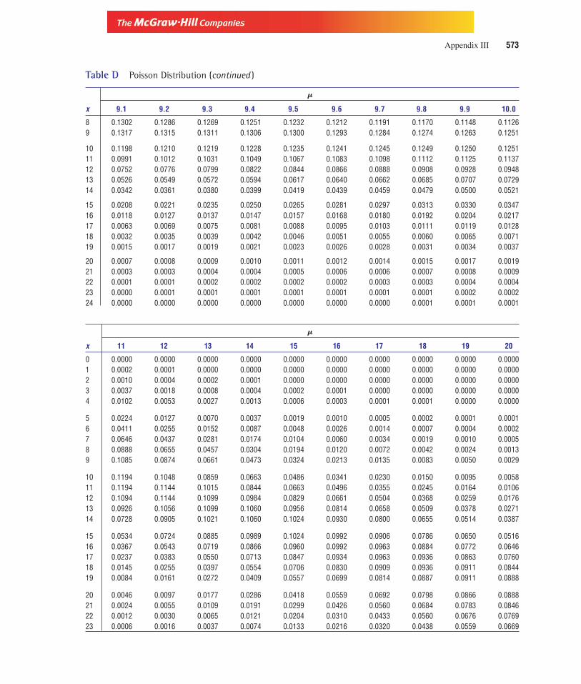
Version, Third Edition
Table D Poisson Distribution (continued )
�
x 9.1 9.2 9.3 9.4 9.5 9.6 9.7 9.8 9.9 10.0
8 0.1302 0.1286 0.1269 0.1251 0.1232 0.1212 0.1191 0.1170 0.1148 0.11269 0.1317 0.1315 0.1311 0.1306 0.1300 0.1293 0.1284 0.1274 0.1263 0.1251
10 0.1198 0.1210 0.1219 0.1228 0.1235 0.1241 0.1245 0.1249 0.1250 0.125111 0.0991 0.1012 0.1031 0.1049 0.1067 0.1083 0.1098 0.1112 0.1125 0.113712 0.0752 0.0776 0.0799 0.0822 0.0844 0.0866 0.0888 0.0908 0.0928 0.094813 0.0526 0.0549 0.0572 0.0594 0.0617 0.0640 0.0662 0.0685 0.0707 0.072914 0.0342 0.0361 0.0380 0.0399 0.0419 0.0439 0.0459 0.0479 0.0500 0.0521
15 0.0208 0.0221 0.0235 0.0250 0.0265 0.0281 0.0297 0.0313 0.0330 0.034716 0.0118 0.0127 0.0137 0.0147 0.0157 0.0168 0.0180 0.0192 0.0204 0.021717 0.0063 0.0069 0.0075 0.0081 0.0088 0.0095 0.0103 0.0111 0.0119 0.012818 0.0032 0.0035 0.0039 0.0042 0.0046 0.0051 0.0055 0.0060 0.0065 0.007119 0.0015 0.0017 0.0019 0.0021 0.0023 0.0026 0.0028 0.0031 0.0034 0.0037
20 0.0007 0.0008 0.0009 0.0010 0.0011 0.0012 0.0014 0.0015 0.0017 0.001921 0.0003 0.0003 0.0004 0.0004 0.0005 0.0006 0.0006 0.0007 0.0008 0.000922 0.0001 0.0001 0.0002 0.0002 0.0002 0.0002 0.0003 0.0003 0.0004 0.000423 0.0000 0.0001 0.0001 0.0001 0.0001 0.0001 0.0001 0.0001 0.0002 0.000224 0.0000 0.0000 0.0000 0.0000 0.0000 0.0000 0.0000 0.0001 0.0001 0.0001
�
x 11 12 13 14 15 16 17 18 19 20
0 0.0000 0.0000 0.0000 0.0000 0.0000 0.0000 0.0000 0.0000 0.0000 0.00001 0.0002 0.0001 0.0000 0.0000 0.0000 0.0000 0.0000 0.0000 0.0000 0.00002 0.0010 0.0004 0.0002 0.0001 0.0000 0.0000 0.0000 0.0000 0.0000 0.00003 0.0037 0.0018 0.0008 0.0004 0.0002 0.0001 0.0000 0.0000 0.0000 0.00004 0.0102 0.0053 0.0027 0.0013 0.0006 0.0003 0.0001 0.0001 0.0000 0.0000
5 0.0224 0.0127 0.0070 0.0037 0.0019 0.0010 0.0005 0.0002 0.0001 0.00016 0.0411 0.0255 0.0152 0.0087 0.0048 0.0026 0.0014 0.0007 0.0004 0.00027 0.0646 0.0437 0.0281 0.0174 0.0104 0.0060 0.0034 0.0019 0.0010 0.00058 0.0888 0.0655 0.0457 0.0304 0.0194 0.0120 0.0072 0.0042 0.0024 0.00139 0.1085 0.0874 0.0661 0.0473 0.0324 0.0213 0.0135 0.0083 0.0050 0.0029
10 0.1194 0.1048 0.0859 0.0663 0.0486 0.0341 0.0230 0.0150 0.0095 0.005811 0.1194 0.1144 0.1015 0.0844 0.0663 0.0496 0.0355 0.0245 0.0164 0.010612 0.1094 0.1144 0.1099 0.0984 0.0829 0.0661 0.0504 0.0368 0.0259 0.017613 0.0926 0.1056 0.1099 0.1060 0.0956 0.0814 0.0658 0.0509 0.0378 0.027114 0.0728 0.0905 0.1021 0.1060 0.1024 0.0930 0.0800 0.0655 0.0514 0.0387
15 0.0534 0.0724 0.0885 0.0989 0.1024 0.0992 0.0906 0.0786 0.0650 0.051616 0.0367 0.0543 0.0719 0.0866 0.0960 0.0992 0.0963 0.0884 0.0772 0.064617 0.0237 0.0383 0.0550 0.0713 0.0847 0.0934 0.0963 0.0936 0.0863 0.076018 0.0145 0.0255 0.0397 0.0554 0.0706 0.0830 0.0909 0.0936 0.0911 0.084419 0.0084 0.0161 0.0272 0.0409 0.0557 0.0699 0.0814 0.0887 0.0911 0.0888
20 0.0046 0.0097 0.0177 0.0286 0.0418 0.0559 0.0692 0.0798 0.0866 0.088821 0.0024 0.0055 0.0109 0.0191 0.0299 0.0426 0.0560 0.0684 0.0783 0.084622 0.0012 0.0030 0.0065 0.0121 0.0204 0.0310 0.0433 0.0560 0.0676 0.076923 0.0006 0.0016 0.0037 0.0074 0.0133 0.0216 0.0320 0.0438 0.0559 0.0669
Appendix III 573

Version, Third Edition
Table D Poisson Distribution (continued )
�
x 11 12 13 14 15 16 17 18 19 20
24 0.0003 0.0008 0.0020 0.0043 0.0083 0.0144 0.0226 0.0328 0.0442 0.0557
25 0.0001 0.0004 0.0010 0.0024 0.0050 0.0092 0.0154 0.0237 0.0336 0.044626 0.0000 0.0002 0.0005 0.0013 0.0029 0.0057 0.0101 0.0164 0.0246 0.034327 0.0000 0.0001 0.0002 0.0007 0.0016 0.0034 0.0063 0.0109 0.0173 0.025428 0.0000 0.0000 0.0001 0.0003 0.0009 0.0019 0.0038 0.0070 0.0117 0.018129 0.0000 0.0000 0.0001 0.0002 0.0004 0.0011 0.0023 0.0044 0.0077 0.0125
30 0.0000 0.0000 0.0000 0.0001 0.0002 0.0006 0.0013 0.0026 0.0049 0.008331 0.0000 0.0000 0.0000 0.0000 0.0001 0.0003 0.0007 0.0015 0.0030 0.005432 0.0000 0.0000 0.0000 0.0000 0.0001 0.0001 0.0004 0.0009 0.0018 0.003433 0.0000 0.0000 0.0000 0.0000 0.0000 0.0001 0.0002 0.0005 0.0010 0.002034 0.0000 0.0000 0.0000 0.0000 0.0000 0.0000 0.0001 0.0002 0.0006 0.0012
35 0.0000 0.0000 0.0000 0.0000 0.0000 0.0000 0.0000 0.0001 0.0003 0.000736 0.0000 0.0000 0.0000 0.0000 0.0000 0.0000 0.0000 0.0001 0.0002 0.000437 0.0000 0.0000 0.0000 0.0000 0.0000 0.0000 0.0000 0.0000 0.0001 0.000238 0.0000 0.0000 0.0000 0.0000 0.0000 0.0000 0.0000 0.0000 0.0000 0.000139 0.0000 0.0000 0.0000 0.0000 0.0000 0.0000 0.0000 0.0000 0.0000 0.0001
574 Statistical Tables

Version, Third Edition
Table E The Normal Distribution
Z 0.00 0.01 0.02 0.03 0.04 0.05 0.06 0.07 0.08 0.09
0.0 0.0000 0.0040 0.0080 0.0120 0.0160 0.0199 0.0239 0.0279 0.0319 0.03590.1 0.0398 0.0438 0.0478 0.0517 0.0557 0.0596 0.0636 0.0675 0.0714 0.07530.2 0.0793 0.0832 0.0871 0.0910 0.0948 0.0987 0.1026 0.1064 0.1103 0.11410.3 0.1179 0.1217 0.1255 0.1293 0.1331 0.1368 0.1406 0.1443 0.1480 0.15170.4 0.1554 0.1591 0.1628 0.1664 0.1700 0.1736 0.1772 0.1808 0.1844 0.1879
0.5 0.1915 0.1950 0.1985 0.2019 0.2054 0.2088 0.2123 0.2157 0.2190 0.22240.6 0.2257 0.2291 0.2324 0.2357 0.2389 0.2422 0.2454 0.2486 0.2517 0.25490.7 0.2580 0.2611 0.2642 0.2673 0.2704 0.2734 0.2764 0.2794 0.2823 0.28520.8 0.2881 0.2910 0.2939 0.2967 0.2995 0.3023 0.3051 0.3078 0.3106 0.31330.9 0.3159 0.3186 0.3212 0.3238 0.3264 0.3289 0.3315 0.3340 0.3365 0.3389
1.0 0.3413 0.3438 0.3461 0.3485 0.3508 0.3531 0.3554 0.3577 0.3599 0.36211.1 0.3643 0.3665 0.3686 0.3708 0.3729 0.3749 0.3770 0.3790 0.3810 0.38301.2 0.3849 0.3869 0.3888 0.3907 0.3925 0.3944 0.3962 0.3980 0.3997 0.40151.3 0.4032 0.4049 0.4066 0.4082 0.4099 0.4115 0.4131 0.4147 0.4162 0.41771.4 0.4192 0.4207 0.4222 0.4236 0.4251 0.4265 0.4279 0.4292 0.4306 0.4319
1.5 0.4332 0.4345 0.4357 0.4370 0.4382 0.4394 0.4406 0.4418 0.4429 0.44411.6 0.4452 0.4463 0.4474 0.4484 0.4495 0.4505 0.4515 0.4525 0.4535 0.45451.7 0.4554 0.4564 0.4573 0.4582 0.4591 0.4599 0.4608 0.4616 0.4625 0.46331.8 0.4641 0.4649 0.4656 0.4664 0.4671 0.4678 0.4686 0.4693 0.4699 0.47061.9 0.4713 0.4719 0.4726 0.4732 0.4738 0.4744 0.4750 0.4756 0.4761 0.4767
2.0 0.4772 0.4778 0.4783 0.4788 0.4793 0.4798 0.4803 0.4808 0.4812 0.48172.1 0.4821 0.4826 0.4830 0.4834 0.4838 0.4842 0.4846 0.4850 0.4854 0.48572.2 0.4861 0.4864 0.4868 0.4871 0.4875 0.4878 0.4881 0.4884 0.4887 0.48902.3 0.4893 0.4896 0.4898 0.4901 0.4904 0.4906 0.4909 0.4911 0.4913 0.49162.4 0.4918 0.4920 0.4922 0.4925 0.4927 0.4929 0.4931 0.4932 0.4934 0.4936
2.5 0.4938 0.4940 0.4941 0.4943 0.4945 0.4946 0.4948 0.4949 0.4951 0.49522.6 0.4953 0.4955 0.4956 0.4957 0.4959 0.4960 0.4961 0.4962 0.4963 0.49642.7 0.4965 0.4966 0.4967 0.4968 0.4969 0.4970 0.4971 0.4972 0.4973 0.49742.8 0.4974 0.4975 0.4976 0.4977 0.4977 0.4978 0.4979 0.4979 0.4980 0.49812.9 0.4981 0.4982 0.4982 0.4983 0.4984 0.4984 0.4985 0.4985 0.4986 0.4986
3.0 0.4987 0.4987 0.4987 0.4988 0.4988 0.4989 0.4989 0.4989 0.4990 0.49903.1 0.4990 0.4991 0.4991 0.4991 0.4992 0.4992 0.4992 0.4992 0.4993 0.49933.2 0.4993 0.4993 0.4994 0.4994 0.4994 0.4994 0.4994 0.4995 0.4995 0.49953.3 0.4995 0.4995 0.4995 0.4996 0.4996 0.4996 0.4996 0.4996 0.4996 0.49973.4 0.4997 0.4997 0.4997 0.4997 0.4997 0.4997 0.4997 0.4997 0.4997 0.4998
3.5 0.4998 0.4998 0.4998 0.4998 0.4998 0.4998 0.4998 0.4998 0.4998 0.44983.6 0.4998 0.4998 0.4999 0.4999 0.4999 0.4999 0.4999 0.4999 0.4999 0.49993.7 0.4999 0.4999 0.4999 0.4999 0.4999 0.4999 0.4999 0.4999 0.4999 0.49993.8 0.4999 0.4999 0.4999 0.4999 0.4999 0.4999 0.4999 0.4999 0.4999 0.49993.9 0.5000 0.5000 0.5000 0.5000 0.5000 0.5000 0.5000 0.5000 0.5000 0.5000
Appendix III 575
P(0 < Z < 1.96) = 0.4750
0.4750
1.96 Z

Version, Third Edition
Table F The t-Distribution
0.900 0.700 0.500 0.300 0.200 0.100 0.050 0.020 0.010 a value Two-0.100 0.300 0.500 0.700 0.800 0.900 0.950 0.980 0.990 CL tailed test
0.450 0.350 0.250 0.150 0.100 0.050 0.025 0.010 0.005 a value One-0.550 0.650 0.750 0.850 0.900 0.950 0.975 0.990 0.995 CL tailed test
d.f. Values of t
1 0.158 0.510 1.000 1.963 3.078 6.314 12.706 31.821 63.6572 0.142 0.445 0.816 1.386 1.886 2.920 4.303 6.965 9.9253 0.137 0.424 0.765 1.250 1.638 2.353 3.182 4.541 5.8414 0.134 0.414 0.741 1.190 1.533 2.132 2.776 3.747 4.6045 0.132 0.408 0.727 1.156 1.476 2.015 2.571 3.365 4.032
6 0.131 0.404 0.718 1.134 1.440 1.943 2.447 3.143 3.7077 0.130 0.402 0.711 1.119 1.415 1.895 2.365 2.998 3.4998 0.130 0.399 0.706 1.108 1.397 1.860 2.306 2.896 3.3559 0.129 0.398 0.703 1.100 1.383 1.833 2.262 2.821 3.25010 0.129 0.397 0.700 1.093 1.372 1.812 2.228 2.764 3.169
11 0.129 0.396 0.697 1.088 1.363 1.796 2.201 2.718 3.10612 0.128 0.395 0.695 1.083 1.356 1.782 2.179 2.681 3.05513 0.128 0.394 0.694 1.079 1.350 1.771 2.160 2.650 3.01214 0.128 0.393 0.692 1.076 1.345 1.761 2.145 2.624 2.97715 0.128 0.393 0.691 1.074 1.341 1.753 2.131 2.602 2.947
16 0.128 0.392 0.690 1.071 1.337 1.746 2.120 2.583 2.92117 0.128 0.392 0.689 1.069 1.333 1.740 2.110 2.567 2.89818 0.127 0.392 0.688 1.067 1.330 1.734 2.101 2.552 2.87819 0.127 0.391 0.688 1.066 1.328 1.729 2.093 2.539 2.86120 0.127 0.391 0.687 1.064 1.325 1.725 2.086 2.528 2.845
21 0.127 0.391 0.686 1.063 1.323 1.721 2.080 2.518 2.83122 0.127 0.390 0.686 1.061 1.321 1.717 2.074 2.508 2.81923 0.127 0.390 0.685 1.060 1.319 1.714 2.069 2.500 2.80724 0.127 0.390 0.685 1.059 1.318 1.711 2.064 2.492 2.79725 0.127 0.390 0.684 1.058 1.316 1.708 2.060 2.485 2.787
26 0.127 0.390 0.684 1.058 1.315 1.706 2.056 2.479 2.77927 0.127 0.389 0.684 1.057 1.314 1.703 2.052 2.473 2.77128 0.127 0.389 0.683 1.056 1.313 1.701 2.048 2.467 2.76329 0.127 0.389 0.683 1.055 1.311 1.699 2.045 2.462 2.75630 0.127 0.389 0.683 1.055 1.310 1.697 2.042 2.457 2.750
40 0.126 0.388 0.681 1.050 1.303 1.684 2.021 2.423 2.70460 0.126 0.387 0.679 1.045 1.296 1.671 2.000 2.390 2.660120 0.126 0.386 0.677 1.041 1.289 1.658 1.980 2.358 2.617� 0.126 0.385 0.674 1.036 1.282 1.645 1.960 2.326 2.576
576 Statistical Tables
Two-tailed test
0.025
0 t
0.025
–2.093 +2.093
t 0.05, 19 = ± 2.093 One-tailed test
0.05
0 1.729
t 0.05, 19 = 1.729
}}

Version, Third Edition
Table G The F-Distribution
F0.90; � 0.10
DenominatorDegrees of Numerator Degrees of FreedomFreedom 1 2 3 4 5 6 7 8 9
1 39.86 49.50 53.59 55.83 57.24 58.20 58.91 59.44 59.862 8.53 9.00 9.16 9.24 9.29 9.33 9.35 9.37 9.383 5.54 5.46 5.39 5.34 5.31 5.28 5.27 5.25 5.244 4.54 4.32 4.19 4.11 4.05 4.01 3.98 3.95 3.94
5 4.06 3.78 3.62 3.52 3.45 3.40 3.37 3.34 3.326 3.78 3.46 3.29 3.18 3.11 3.05 3.01 2.98 2.967 3.59 3.26 3.07 2.96 2.88 2.83 2.78 2.75 2.728 3.46 3.11 2.92 2.81 2.73 2.67 2.62 2.59 2.569 3.36 3.01 2.81 2.69 2.61 2.55 2.51 2.47 2.44
10 3.29 2.92 2.13 2.61 2.52 2.46 2.41 2.38 2.3511 3.23 2.86 2.66 2.54 2.45 2.39 2.34 2.30 2.2712 3.18 2.81 2.61 2.48 2.39 2.33 2.28 2.24 2.2113 3.14 2.76 2.56 2.43 2.35 2.28 2.23 2.20 2.1614 3.10 2.73 2.52 2.39 2.31 2.24 2.19 2.15 2.12
15 3.07 2.70 2.49 2.36 2.27 2.21 2.16 2.12 2.0916 3.05 2.67 2.46 2.33 2.24 2.18 2.13 2.09 2.0617 3.03 2.64 2.44 2.31 2.22 2.15 2.10 2.06 2.0318 3.01 2.62 2.42 2.29 2.20 2.13 2.08 2.04 2.0019 2.99 2.61 2.40 2.27 2.18 2.11 2.06 2.02 1.98
20 2.97 2.59 2.38 2.25 2.16 2.09 2.04 2.00 1.9621 2.96 2.57 2.36 2.23 2.14 2.08 2.02 1.98 1.9522 2.95 2.56 2.35 2.22 2.13 2.06 2.01 1.97 1.9323 2.94 2.55 2.34 2.21 2.11 2.05 1.99 1.95 1.9224 2.93 2.54 2.33 2.19 2.10 2.04 1.98 1.94 1.91
25 2.92 2.53 2.32 2.18 2.09 2.02 1.97 1.93 1.8926 2.91 2.52 2.31 2.17 2.08 2.01 1.96 1.92 1.8827 2.90 2.51 2.30 2.17 2.07 2.00 1.95 1.91 1.8728 2.89 2.50 2.29 2.16 2.06 2.00 1.94 1.90 1.8729 2.89 2.50 2.28 2.15 2.06 1.99 1.93 1.89 1.86
30 2.88 2.49 2.28 2.14 2.05 1.98 1.93 1.88 1.8540 2.84 2.44 2.23 2.09 2.00 1.93 1.87 1.83 1.7960 2.79 2.39 2.18 2.04 1.95 1.87 1.82 1.77 1.74120 2.75 2.35 2.13 1.99 1.90 1.82 1.77 1.72 1.68� 2.71 2.30 2.08 1.95 1.85 1.77 1.72 1.67 1.63
Appendix III 577
0.10
0 3.52P(F4,5 ≤ 3.52) = 0.90
f (F )
F

Version, Third Edition
Table G The F-Distribution (continued)
F0.90; � 0.10
DenominatorDegrees of Numerator Degrees of FreedomFreedom 10 12 15 20 24 30 40 60 120 �
1 60.19 60.71 61.22 61.74 62.00 62.26 62.53 62.79 63.06 63.332 9.39 9.41 9.42 9.44 9.45 9.46 9.47 9.47 9.48 9.493 5.23 5.22 5.20 5.18 5.18 5.17 5.16 5.15 5.14 5.134 3.92 3.90 3.87 3.84 3.83 3.82 3.80 3.79 3.78 3.76
5 3.30 3.27 3.24 3.21 3.19 3.17 3.16 3.14 3.12 3.116 2.94 2.90 2.87 2.84 2.82 2.80 2.78 2.76 2.74 2.727 2.70 2.67 2.63 2.59 2.58 2.56 2.54 2.51 2.49 2.478 2.54 2.50 2.46 2.42 2.40 2.38 2.36 2.34 2.32 2.299 2.42 2.38 2.34 2.30 2.28 2.25 2.23 2.21 2.18 2.16
10 2.32 2.28 2.24 2.20 2.18 2.16 2.13 2.11 2.08 2.0611 2.25 2.21 2.17 2.12 2.10 2.08 2.05 2.03 2.00 1.9712 2.19 2.15 2.10 2.06 2.04 2.01 1.99 1.96 1.93 1.9013 2.14 2.10 2.05 2.01 1.98 1.96 1.93 1.90 1.88 1.8514 2.10 2.05 2.01 1.96 1.94 1.91 1.89 1.86 1.83 1.80
15 2.06 2.02 1.97 1.92 1.90 1.87 1.85 1.82 1.79 1.7616 2.03 1.99 1.94 1.89 1.87 1.84 1.81 1.78 1.75 1.7217 2.00 1.96 1.91 1.86 1.84 1.81 1.78 1.75 1.72 1.6918 1.98 1.93 1.89 1.84 1.81 1.78 1.75 1.72 1.69 1.6619 1.96 1.91 1.86 1.81 1.79 1.76 1.73 1.70 1.67 1.63
20 1.94 1.89 1.84 1.79 1.77 1.74 1.71 1.68 1.64 1.6121 1.92 1.87 1.83 1.78 1.75 1.72 1.69 1.66 1.62 1.5922 1.90 1.86 1.81 1.76 1.73 1.70 1.67 1.64 1.60 1.5723 1.89 1.84 1.80 1.74 1.72 1.69 1.66 1.62 1.59 1.5524 1.88 1.83 1.78 1.73 1.70 1.67 1.64 1.61 1.57 1.53
25 1.87 1.82 1.77 1.72 1.69 1.66 1.63 1.59 1.56 1.5226 1.86 1.81 1.76 1.71 1.68 1.65 1.61 1.58 1.54 1..5027 1.85 1.80 1.75 1.70 1.67 1.64 1.60 1.57 1.53 1.4928 1.84 1.79 1.74 1.69 1.66 1.63 1.59 1.56 1.52 1.4829 1.83 1.78 1.73 1.68 1.65 1.62 1.58 1.55 1.51 1.47
30 1.82 1.77 1.72 1.67 1.64 1.61 1.57 1.54 1.50 1.4640 1.76 1.71 1.66 1.61 1.57 1.54 1.51 1.47 1.42 1.3860 1.71 1.66 1.60 1.54 1.51 1.48 1.44 1.40 1.35 1.29120 1.65 1.60 1.55 1.48 1.45 1.41 1.37 1.32 1.26 1.19� 1.60 1.55 1.49 1.42 1.38 1.34 1.30 1.24 1.17 1.00
F0.95; � 0.05
DenominatorDegrees of Numerator Degrees of FreedomFreedom 1 2 3 4 5 6 7 8 9
1 161.45 199.50 215.71 224.58 230.16 233.99 236.77 238.88 240.542 18.51 19.00 19.16 19.25 19.30 19.33 19.35 19.37 19.383 10.13 9.55 9.28 9.12 9.01 8.94 8.89 8.85 8.814 7.71 6.94 6.59 6.39 6.26 6.16 6.09 6.04 6.00
578 Statistical Tables

Version, Third Edition
Table G The F-Distribution (continued)
F0.95; � 0.05
DenominatorDegrees of Numerator Degrees of FreedomFreedom 1 2 3 4 5 6 7 8 9
5 6.61 5.79 5.41 5.19 5.05 4.95 4.88 4.82 4.776 5.99 5.14 4.76 4.53 4.39 4.28 4.21 4.15 4.107 5.59 4.74 4.35 4.12 3.97 3.87 3.79 3.73 3.688 5.32 4.46 4.07 3.84 3.69 3.58 3.50 3.44 3.399 5.12 4.26 3.86 3.63 3.48 3.37 3.29 3.23 3.18
10 4.96 4.10 3.71 3.48 3.33 3.22 3.14 3.07 3.0211 4.84 3.98 3.59 3.36 3.20 3.09 3.01 2.95 2.9012 4.75 3.89 3.49 3.26 3.11 3.00 2.91 2.85 2.8013 4.67 3.81 3.41 3.18 3.03 2.92 2.83 2.77 2.7114 4.60 3.74 3.34 3.11 2.96 2.85 2.76 2.70 2.65
15 4.54 3.68 3.29 3.06 2.90 2.79 2.71 2.64 2.5916 4.49 3.63 3.24 3.01 2.85 2.74 2.66 2.59 2.5417 4.45 3.59 3.20 2.96 2.81 2.70 2.61 2.55 2.4918 4.41 3.55 3.16 2.93 2.77 2.66 2.58 2.51 2.4619 4.38 3.52 3.13 2.90 2.74 2.63 2.54 2.48 2.42
20 4.35 3.49 3.10 2.87 2.71 2.60 2.51 2.45 2.3921 4.32 3.47 3.07 2.84 2.68 2.57 2.49 2.42 2.3722 4.30 3.44 3.05 2.82 2.66 2.55 2.46 2.40 2.3423 4.28 3.42 3.03 2.80 2.64 2.53 2.44 2.37 2.3224 4.26 3.40 3.01 2.78 2.62 2.51 2.42 2.36 2.30
25 4.24 3.39 2.99 2.76 2.60 2.49 2.40 2.34 2.2826 4.23 3.37 2.98 2.74 2.59 2.47 2.39 2.32 2.2727 4.21 3.35 2.96 2.73 2.57 2.46 2.37 2.31 2.2528 4.20 3.34 2.95 2.71 2.56 2.45 2.36 2.29 2.2429 4.18 3.33 2.93 2.70 2.55 2.43 2.35 2.28 2.22
30 4.17 3.32 2.92 2.69 2.53 2.42 2.33 2.27 2.2140 4.08 3.23 2.84 2.61 2.45 2.34 2.25 2.18 2.1260 4.00 3.15 2.76 2.53 2.37 2.25 2.17 2.10 2.04120 3.92 3.07 2.68 2.45 2.29 2.18 2.09 2.02 1.96� 3.84 3.00 2.61 2.37 2.21 2.10 2.01 1.94 1.88
F0.95; � 0.05
DenominatorDegrees of Numerator Degrees of FreedomFreedom 10 12 15 20 24 30 40 60 120 �
1 241.88 243.91 245.95 248.01 249.05 250.10 251.14 252.20 253.25 254.312 19.40 19.41 19.43 19.45 19.45 19.46 19.47 19.48 19.49 19.503 8.79 8.74 8.70 8.66 8.64 8.62 8.59 8.57 8.55 8..534 5.96 5.91 5.86 5.80 5.77 5.75 5.72 5.69 5.66 5.63
5 4.74 4.68 4.62 4.56 4.53 4.50 4.46 4.43 4.40 4.376 4.06 4.00 3.94 3.87 3.84 3.81 3.77 3.74 3.70 3.677 3.64 3.57 3.51 3.44 3.41 3.38 3.34 3.30 3.27 3.238 3.35 3.28 3.22 3.15 3.12 3.08 3.04 3.01 2.97 2.939 3.14 3.07 3.01 2.94 2.90 2.86 2.83 2.79 2.75 2.71
Appendix III 579

Version, Third Edition
Table G The F-Distribution (continued)
F0.95; � 0.05
DenominatorDegrees of Numerator Degrees of FreedomFreedom 10 12 15 20 24 30 40 60 120 �
10 2.98 2.91 2.85 2.77 2.74 2.70 2.66 2.62 2.58 2.5411 2.85 2.79 2.72 2.65 2.61 2.57 2.53 2.49 2.45 2.4012 2.75 2.69 2.62 2.54 2.51 2.47 2.43 2.38 2.34 2.3013 2.67 2.60 2.53 2.46 2.42 2.38 2.34 2.30 2.25 2.2114 2.60 2.53 2.46 2.39 2.35 2.31 2.27 2.22 2.18 2.13
15 2.54 2.48 2.40 2.33 2.29 2.25 2.20 2.16 2.11 2.0716 2.49 2.42 2.35 2.28 2.24 2.19 2.15 2.11 2.06 2.0117 2.45 2.38 2.31 2.23 2.19 2.15 2.10 2.06 2.01 1.9618 2.41 2.34 2.27 2.19 2.15 2.11 2.06 2.02 1.97 1.9219 2.38 2.31 2.23 2.16 2.11 2.07 2.03 1.98 1.93 1.88
20 2.35 2.28 2.20 2.12 2.08 2.04 1.99 1.95 1.90 1.8421 2.32 2.25 2.18 2.10 2.05 2.01 1.96 1.92 1.87 1.8122 2.30 2.23 2.15 2.07 2.03 1.98 1.94 1.89 1.84 1.7823 2.27 2.20 2.13 2.05 2.01 1.96 1.91 1.86 1.81 1.7624 2.25 2.18 2.11 2.03 1.98 1.94 1.89 1.84 1.79 1.73
25 2.24 2.16 2.09 2.01 1.96 1.92 1.87 1.82 1.77 1.7126 2.22 2.15 2.07 1.99 1.95 1.90 1.85 1.80 1.75 1.6927 2.20 2.13 2.06 1.97 1.93 1.88 1.84 1.79 1.73 1.6728 2.19 2.12 2.04 1.96 1.91 1.87 1.82 1.77 1.71 1.6529 2.18 2.10 2.03 1.94 1.90 1.85 1.81 1.75 1.70 1.64
30 2.16 2.09 2.01 1.93 1.89 1.84 1.79 1.74 1.68 1.6240 2.08 2.00 1.92 1.84 1.79 1.74 1.69 1.64 1.58 1.5160 1.99 1.92 1.84 1.75 1.70 1.65 1.59 1.53 1.47 1.39120 1.91 1.83 1.75 1.66 1.61 1.55 1.50 1.43 1.35 1.25� 1.83 1.75 1.67 1.57 1.52 1.46 1.39 1.32 1.22 1.00
F0.975; � 0.025
DenominatorDegrees of Numerator Degrees of FreedomFreedom 1 2 3 4 5 6 7 8 9
1 647.8 799.5 864.2 899.6 921.8 937.1 948.2 956.7 963.32 38.51 39.00 39.17 39.25 39.30 39.33 39.36 39.37 39.393 17.44 16.04 15.44 15.10 14.88 14.73 14.62 14.54 14.474 12.22 10.65 9.98 9.60 9.36 9.20 9.07 8.98 8.90
5 10.01 8.43 7.76 7.39 7.15 6.98 6.85 6.76 6.686 8.81 7.26 6.60 6.23 5.99 5.82 5.70 5.60 5.527 8.07 6.54 5.89 5.52 5.29 5.12 4.99 4.90 4.828 7.57 6.06 5.42 5.05 4.82 4.65 4.53 4.43 4.369 7.21 5.71 5.08 4.72 4.48 4.32 4.20 4.10 4.03
10 6.94 5.46 4.83 4.47 4.24 4.07 3.95 3.85 3.7811 6.72 5.26 4.63 4.28 4.04 3.88 3.76 3.66 3.5912 6.55 5.10 4.47 4.12 3.89 3.73 3.61 3.51 3.4413 6.41 4.97 4.35 4.00 3.77 3.60 3.48 3.39 3.31
580 Statistical Tables

Version, Third Edition
Table G The F-Distribution (continued)
F0.975; � 0.025
DenominatorDegrees of Numerator Degrees of FreedomFreedom 1 2 3 4 5 6 7 8 9
14 6.30 4.86 4.24 3.89 3.66 3.50 3.38 3.29 3.21
15 6.20 4.77 4.15 3.80 3.58 3.41 3.29 3.20 3.1216 6.12 4.69 4.08 3.73 3.50 3.34 3.22 3.12 3.0517 6.04 4.62 4.01 3.66 3.44 3.28 3.16 3.06 2.9818 5.98 4.56 3.95 3.61 3.38 3.22 3.10 3.01 2.9319 5.92 4.51 3.90 3.56 3.33 3.17 3.05 2.96 2.88
20 5.87 4.46 3.86 3.51 3.29 3.13 3.01 2.91 2.8421 5.83 4.42 3.82 3.48 3.25 3.09 2.97 2.87 2.8022 5.79 4.38 3.78 3.44 3.22 3.05 2.93 2.84 2.7623 5.75 4.35 3.75 3.41 3.18 3.02 2.90 2.81 2.7324 5.72 4.32 3.72 3.38 3.15 2.99 2.87 2.78 2.70
25 5.69 4.29 3.69 3.35 3.13 2.97 2.85 2.75 2.6826 5.66 4.27 3.67 3.33 3.10 2.94 2.82 2.73 2.6527 5.63 4.24 3.65 3.31 3.08 2.92 2.80 2.71 2.6328 5.61 4.22 3.63 3.29 3.06 2.90 2.78 2.69 2.6129 5.59 4.20 3.61 3.27 3.04 2.88 2.76 2.67 2.59
30 5.57 4.18 3.59 3.25 3.03 2.87 2.75 2.65 2.5740 5.42 4.05 3.46 3.13 2.90 2.74 2.62 2.53 2.4560 5.29 3.93 3.34 3.01 2.79 2.63 2.51 2.41 2.33120 5.15 3.80 3.23 2.89 2.67 2.52 2.39 2.30 2.22� 5.02 3.69 3.12 2.79 2.57 2.41 2.29 2.19 2.11
F0.975; � 0.025
DenominatorDegrees of Numerator Degrees of FreedomFreedom 10 12 15 20 24 30 40 60 120 �
1 968.6 976.7 984.9 993.1 997.2 1001.4 1005.6 1009.8 1014.0 1018.22 39.40 39.41 39.43 39.45 39.46 39.46 39.47 39.48 39.49 39.503 14.42 14.34 14.25 14.17 14.12 14.08 14.04 13.99 13.95 13.904 8.84 8.75 8.66 8.56 8.51 8.46 8.41 8.36 8.31 8.26
5 6.62 6.52 6.43 6.33 6.28 6.23 6.18 6.12 6.07 6.026 5.46 5.37 5.27 5.17 5.12 5.07 5.01 4.96 4.90 4.857 4.76 4.67 4.57 4.47 4.41 4.36 4.31 4.25 4.20 4.148 4.30 4.20 4.10 4.00 3.95 3.89 3.84 3.78 3.73 3.679 3.96 3.87 3.77 3.67 3.61 3.56 3.51 3.45 3.39 3.33
10 3.72 3.62 3.52 3.42 3.37 3.31 3.26 3.20 3.14 3.0811 3.53 3.43 3.33 3.23 3.17 3.12 3.06 3.00 2.94 2.8812 3.37 3.28 3.18 3.07 3.02 2.96 2.91 2.85 2.79 2.7313 3.25 3.15 3.05 2.95 2.89 2.84 2.78 2.72 2.66 2.6014 3.15 3.05 2.95 2.84 2.79 2.73 2.67 2.61 2.55 2.49
15 3.06 2.96 2.86 2.76 2.70 2.64 2.59 2.52 2.46 2.4016 2.99 2.89 2.79 2.68 2.63 2.57 2.51 2.45 2.38 2.32
Appendix III 581

Version, Third Edition
Table G The F-Distribution (continued)
F0.975; � 0.025
DenominatorDegrees of Numerator Degrees of FreedomFreedom 10 12 15 20 24 30 40 60 120 �
17 2.92 2.82 2.72 2.62 2.56 2.50 2.44 2.38 2.32 2.2518 2.87 2.77 2.67 2.56 2.50 2.44 2.38 2.32 2.26 2.1919 2.82 2.72 2.62 2.51 2.45 2.39 2.33 2.27 2.20 2.13
20 2.77 2.68 2.57 2.46 2.41 2.35 2.29 2.22 2.16 2.0921 2.73 2.64 2.53 2.42 2.37 2.31 2.25 2.18 2.11 2.0422 2.70 2.60 2.50 2.39 2.33 2.27 2.21 2.14 2.08 2.0023 2.67 2.57 2.47 2.36 2.30 2.24 2.18 2.11 2.04 1.9724 2.64 2.54 2.44 2.33 2.27 2.21 2.15 2.08 2.01 1.94
25 2.61 2.51 2.41 2.30 2.24 2.18 2.12 2.05 1.98 1.9126 2.59 2.49 2.39 2.28 2.22 2.16 2.09 2.03 1.95 1.8827 2.57 2.47 2.36 2.25 2.19 2.13 2.07 2.00 1.93 1.8528 2.55 2.45 2.34 2.23 2.17 2.11 2.05 1.98 1.91 1.8329 2.53 2.43 2.32 2.21 2.15 2.09 2.03 1.96 1.89 1.81
30 2.51 2.41 2.31 2.20 2.14 2.07 2.01 1.94 1.87 1.7940 2.39 2.29 2.18 2.07 2.01 1.94 1.88 1.80 1.72 1.6460 2.27 2.17 2.06 1.94 1.88 1.82 1.74 1.67 1.58 1.48120 2.16 2.05 1.94 1.82 1.76 1.69 1.61 1.53 1.43 1.31� 2.05 1.95 1.83 1.71 1.64 1.57 1.48 1.39 1.27 1.00
F0.99; � 0.01
DenominatorDegrees of Numerator Degrees of FreedomFreedom 1 2 3 4 5 6 7 8 9
1 4052.2 4999.5 5403.4 5624.6 5763.6 5859.0 5928.4 5981.1 6022.52 98.50 99.00 99.17 99.25 99.30 99.33 99.36 99.37 99.393 34.12 30.82 29.46 28.71 28.24 27.91 27.67 27.49 27.354 21.20 18.00 16.69 15.98 15.52 15.21 14.98 14.80 14.66
5 16.26 13.27 12.06 11.39 10.97 10.67 10.46 10.29 10.166 13.75 10.92 9.78 9.15 8.75 8.47 8.26 8.10 7.987 12.25 9.55 8.45 7.85 7.46 7.19 6.99 6.84 6.728 11.26 8.65 7.59 7.01 6.63 6.37 6.18 6.03 5.919 10.56 8.02 6.99 6.42 6.06 5.80 5.61 5.47 5.35
10 10.04 7.56 6.55 5.99 5.64 5.39 5.20 5.06 4.9411 9.65 7.21 6.22 5.67 5.32 5.07 4.89 4.74 4.6312 9.33 6.93 5.95 5.41 5.06 4.82 4.64 4.50 4.3913 9.07 6.70 5.74 5.21 4.86 4.62 4.44 4.30 4.1914 8.86 6.51 5.56 5.04 4.69 4.46 4.28 4.14 4.03
15 8.68 6.36 5.42 4.89 4.56 4.32 4.14 4.00 3.8916 8.53 6.23 5.29 4.77 4.44 4.20 4.03 3.89 3.7817 8.40 6.11 5.18 4.67 4.34 4.10 3.93 3.79 3.6818 8.29 6.01 5.09 4.58 4.25 4.01 3.84 3.71 3.6019 8.18 5.93 5.01 4.50 4.17 3.94 3.77 3.63 3.52
582 Statistical Tables

Version, Third Edition
Table G The F-Distribution (continued)
F0.99; � 0.01
DenominatorDegrees of Numerator Degrees of FreedomFreedom 1 2 3 4 5 6 7 8 9
20 8.10 5.85 4.94 4.43 4.10 3.87 3.70 3.56 3.4621 8.02 5.78 4.87 4.37 4.04 3.81 3.64 3.51 3.4022 7.95 5.72 4.82 4.31 3.99 3.76 3.59 3.45 3.3523 7.88 5.66 4.76 4.26 3.94 3.71 3.54 3.41 3.3024 7.82 5.61 4.72 4.22 3.90 3.67 3.50 3.36 3.26
25 7.77 5.57 4.68 4.18 3.85 3.63 3.46 3.32 3.2226 7.72 5.53 4.64 4.14 3.82 3.59 3.42 3.29 3.1827 7.68 5.49 4.60 4.11 3.78 3.56 3.39 3.26 3.1528 7.64 5.45 4.57 4.07 3.75 3.53 3.36 3.23 3.1229 7.60 5.42 4.54 4.04 3.73 3.50 3.33 3.20 3.09
30 7.56 5.39 4.51 4.02 3.70 3.47 3.30 3.17 3.0740 7.31 5.18 4.31 3.83 3.51 3.29 3.12 2.99 2.8960 7.08 4.98 4.13 3.65 3.34 3.12 2.95 2.82 2.72120 6.85 4.79 3.95 3.48 3.17 2.96 2.79 2.66 2.56� 6.64 4.61 3.78 3.32 3.02 2.80 2.64 2.51 2.41
F0.99; � 0.01
DenominatorDegrees of Numerator Degrees of FreedomFreedom 10 12 15 20 24 30 40 60 120 �
1 6055.8 6106.3 6157.3 6208.7 6234.6 6260.6 6286.8 6313.0 6339.4 6365.82 99.40 99.42 99.43 99.45 99.46 99.47 99.47 99.48 99.49 99.503 27.23 27.05 26.87 26.69 26.60 26.50 26.41 26.32 26.22 26.134 14.55 14.37 14.20 14.02 13.93 13.84 13.75 13.65 13.56 13.46
5 10.05 9.89 9.72 9.55 9.47 9.38 9.29 9.20 9.11 9.026 7.87 8.72 7.56 7.40 7.31 7.23 7.14 7.06 6.97 6.887 6.62 6.47 6.31 6.16 6.07 5.99 5.91 5.82 5.74 5.658 5.81 5.67 5.52 5.36 5.28 5.20 5.12 5.03 4.95 4.869 5.26 5.11 4.96 4.81 4.73 4.65 4.57 4.48 4.40 4.31
10 4.85 4.71 4.56 4.41 4.33 4.25 4.17 4.08 4.00 3.9111 4.54 4.40 4.25 4.10 4.02 3.94 3.86 3.78 3.69 3.6012 4.30 4.16 4.01 3.86 3.78 3.70 3.62 3.54 3.45 3.3613 4.10 3.96 3.82 3.66 3.59 3.51 3.43 3.34 3.25 3.1714 3.94 3.80 3.66 3.51 3.43 3.35 3.27 3.18 3.09 3.00
15 3.80 3.67 3.52 3.37 3.29 3.21 3.13 3.05 2.96 2.8716 3.69 3.55 3.41 3.26 3.18 3.10 3.02 2.93 2.84 2.7517 3.59 3.46 3.31 3.16 3.08 3.00 2.92 2.83 2.75 2.6518 3.51 3.37 3.23 3.08 3.00 2.92 2.84 2.75 2.66 2.5719 3.43 3.30 3.15 3.00 2.92 2.84 2.76 2.67 2.58 2.49
20 3.37 3.23 3.09 2.94 2.86 2.78 2.69 2.61 2.52 2.4221 3.31 3.17 3.03 2.88 2.80 2.72 2.64 2.55 2.46 2.3622 3.26 3.12 2.98 2.83 2.75 2.67 2.58 2.50 2.40 2.3123 3.21 3.07 2.93 2.78 2.70 2.62 2.54 2.45 2.35 2.2624 3.17 3.03 2.89 2.74 2.66 2.58 2.49 2.40 2.31 2.21
Appendix III 583

Version, Third Edition
Table G The F-Distribution (continued)
F0.99; � 0.01
DenominatorDegrees of Numerator Degrees of FreedomFreedom 10 12 15 20 24 30 40 60 120 �
25 3.13 2.99 2.85 2.70 2.62 2.54 2.45 2.36 2.27 2.1726 3.09 2.96 2.81 2.66 2.58 2.50 2.42 2.33 2.23 2.1327 3.06 2.93 2.78 2.63 2.55 2.47 2.38 2.29 2.20 2.1028 3.03 2.90 2.75 2.60 2.52 2.44 2.35 2.26 2.17 2.0629 3.00 2.87 2.73 2.57 2.49 2.41 2.33 2.23 2.14 2.03
30 2.98 2.84 2.70 2.55 2.47 2.39 2.30 2.21 2.11 2.0140 2.80 2.66 2.52 2.37 2.29 2.20 2.11 2.02 1.92 1.8160 2.63 2.50 2.35 2.20 2.12 2.03 1.94 1.84 1.73 1.60120 2.47 2.34 2.19 2.03 1.95 1.86 1.76 1.66 1.53 1.38� 2.32 2.19 2.04 1.88 1.79 1.70 1.59 1.47 1.33 1.00
F0.995; � 0.005
DenominatorDegrees of Numerator Degrees of FreedomFreedom 1 2 3 4 5 6 7 8 9
1 16211 20000 21615 22500 23056 23437 23715 23925 240912 198.50 199.00 199.17 199.25 199.30 199.33 199.36 199.37 199.393 55.55 49.80 47.47 46.19 45.39 44.84 44.43 44.13 43.884 31.33 26.28 24.26 23.15 22.46 21.97 21.62 21.35 21.14
5 22.78 18.31 16.53 15.56 14.94 14.51 14.20 13.96 13.776 18.63 14.54 12.92 12.03 11.46 11.07 10.79 10.57 10.397 16.24 12.40 10.88 10.05 9.52 9.16 8.89 8.68 8.518 14.69 11.04 9.60 8.81 8.30 7.95 7.69 7.50 7.349 13.61 10.11 8.72 7.96 7.47 7.13 6.88 6.69 6.54
10 12.83 9.43 8.08 7.34 6.87 6.54 6.30 6.12 5.9711 12.23 8.91 7.60 6.88 6.42 6.10 5.86 5.68 5.5412 11.75 8.51 7.23 6.52 6.07 5.76 5.52 5.35 5.2013 11.37 8.19 6.93 6.23 5.79 5.48 5.25 5.08 4.9414 11.06 7.92 6.68 6.00 5.56 5.26 5.03 4.86 4.72
15 10.80 7.70 6.48 5.80 5.37 5.07 4.85 4.67 4.5416 10.58 7.51 6.30 5.64 5.21 4.91 4.69 4.52 4.3817 10.38 7.35 6.16 5.50 5.07 4.78 4.56 4.39 4.2518 10.22 7.21 6.03 5.37 4.96 4.66 4.44 4.28 4.1419 10.07 7.09 5.92 5.27 4.85 4.56 4.34 4.18 4.04
20 9.94 6.99 5.82 5.17 4.76 4.47 4.26 4.09 3.9621 9.83 6.89 5.73 5.09 4.68 4.39 4.18 4.01 3.8822 9.73 6.81 5.65 5.02 4.61 4.32 4.11 3.94 3.8123 9.63 6.73 5.58 4.95 4.54 4.26 4.05 3.88 3.7524 9.55 6.66 5.52 4.89 4.49 4.20 3.99 3.83 3.69
25 9.48 6.60 5.46 4.84 4.43 4.15 3.94 3.78 3.6426 9.41 6.54 5.41 4.79 4.38 4.10 3.89 3.73 3.6027 9.34 6.49 5.36 4.74 4.34 4.06 3.85 3.69 3.5628 9.28 6.44 5.32 4.70 4.30 4.02 3.81 3.65 3.5229 9.23 6.40 5.28 4.66 4.26 3.98 3.77 3.61 3.48
584 Statistical Tables

Version, Third Edition
Table G The F-Distribution (concluded )
F0.995; � 0.005
DenominatorDegrees of Numerator Degrees of FreedomFreedom 1 2 3 4 5 6 7 8 9
30 9.18 6.35 5.24 4.62 4.23 3.95 3.74 3.58 3.4540 8.83 6.07 4.98 4.37 3.99 3.71 3.51 3.35 3.2260 8.49 5.79 4.73 4.14 3.76 3.49 3.29 3.13 3.01
120 8.18 5.54 4.50 3.92 3.55 3.28 3.09 2.93 2.81� 7.88 5.30 4.28 3.72 3.35 3.09 2.90 2.75 2.62
F0.995; � 0.005
DenominatorDegrees of Numerator Degrees of FreedomFreedom 10 12 15 20 24 30 40 60 120 �
1 24224 24426 24630 24836 24940 25044 25148 25253 25359 254642 199.40 199.42 199.43 199.45 199.46 199.47 199.47 199.48 199.49 199.503 43.69 43.39 43.08 42.78 42.62 42.47 42.31 42.15 41.99 41.834 20.97 20.70 20.44 20.17 20.03 19.89 19.75 19.61 19.47 19.33
5 13.62 13.38 13.15 12.90 12.78 12.66 12.53 12.40 12.27 12.146 10.25 10.03 9.81 9.59 9.47 9.36 9.24 9.12 9.00 8.887 8.38 8.18 7.97 7.75 7.64 7.53 7.42 7.31 7.19 7.088 7.21 7.01 6.81 6.61 6.50 6.40 6.29 6.18 6.06 5.959 6.42 6.23 6.03 5.83 5.73 5.62 5.52 5.41 5.30 5.19
10 5.85 5.66 5.47 5.27 5.17 5.07 4.97 4.86 4.75 4.6411 5.42 5.24 5.05 4.86 4.76 4.65 4.55 4.45 4.34 4.2312 5.09 4.91 4.72 4.53 4.43 4.33 4.23 4.12 4.01 3.9013 4.82 4.64 4.46 4.27 4.17 4.07 3.97 3.87 3.76 3.6514 4.60 4.43 4.25 4.06 3.96 3.86 3.76 3.66 3.55 3.44
15 4.42 4.25 4.07 3.88 3.79 3.69 3.58 3.48 3.37 3.2616 4.27 4.10 3.92 3.73 3.64 3.54 3.44 3.33 3.22 3.1117 4.14 3.97 3.79 3.61 3.51 3.41 3.31 3.21 3.10 2.9818 4.03 3.86 3.68 3.50 3.40 3.30 3.20 3.10 2.99 2.8719 3.93 3.76 3.59 3.40 3.31 3.21 3.11 3.00 2.89 2.78
20 3.85 3.68 3.50 3.32 3.22 3.12 3.02 2.92 2.81 2.6921 3.77 3.60 3.43 3.24 3.15 3.05 2.95 2.84 2.73 2.6122 3.70 3.54 3.36 3.18 3.08 2.98 2.88 2.77 2.66 2.5523 3.64 3.47 3.30 3.12 3.02 2.92 2.82 2.71 2.60 2.4824 3.59 3.42 3.25 3.06 2.97 2.87 2.77 2.66 2.55 2.43
25 3.54 3.37 3.20 3.01 2.92 2.82 2.72 2.61 2.50 2.3826 3.49 3.33 3.15 2.97 2.87 2.77 2.67 2.56 2.45 2.3327 3.45 3.28 3.11 2.93 2.83 2.73 2.63 2.52 2.41 2.2928 3.41 3.25 3.07 2.89 2.79 2.69 2.59 2.48 2.37 2.2529 3.38 3.21 3.04 2.86 2.76 2.66 2.56 2.45 2.33 2.21
30 3.34 3.18 3.01 2.82 2.73 2.63 2.52 2.42 2.30 2.1840 3.12 2.95 2.78 2.60 2.50 2.40 2.30 2.18 2.06 1.9360 2.90 2.74 2.57 2.39 2.29 2.19 2.08 1.96 1.83 1.69120 2.71 2.54 2.37 2.19 2.09 1.98 1.87 1.75 1.61 1.43� 2.52 2.36 2.19 2.00 1.90 1.79 1.67 1.53 1.36 1.00
Appendix III 585

Version, Third Edition
Table H Chi-Square Distribution
d.f. �20.995 �2
0.900 �20.975 �2
0.950 �20.900 �2
0.700 �20.500 �2
0.300 �20.200 �2
0.100 �20.050 �2
0.025 �20.020 �2
0.010 �20.005
1 0.000 0.000 0.001 0.004 0.016 0.148 0.455 1.074 1.642 2.706 3.841 5.024 5.412 6.635 7.8792 0.010 0.020 0.051 0.103 0.211 0.713 1.386 2.408 3.219 4.605 5.991 7.378 7.824 9.210 10.5973 0.072 0.115 0.216 0.352 0.584 1.424 2.366 3.665 4.642 6.251 7.815 9.348 9.837 11.345 12.8384 0.207 0.297 0.484 0.711 1.064 2.195 3.357 4.878 5.989 7.779 9.488 11.143 11.668 13.277 14.860
5 0.412 0.554 0.831 1.145 1.610 3.000 4.351 6.064 7.289 9.236 11.070 12.833 13.388 15.086 16.7506 0.676 0.872 1.237 1.635 2.204 3.828 5.348 7.231 8.558 10.645 12.592 14.449 15.033 16.812 18.5487 0.989 1.239 1.690 2.167 2.833 4.671 6.346 8.383 9.803 12.017 14.067 16.013 16.622 18.475 20.2788 1.344 1.646 2.180 2.733 3.490 5.527 7.344 9.524 11.030 13.362 15.507 17.535 18.168 20.090 21.9559 1.735 2.088 2.700 3.325 4.168 6.393 8.343 10.656 12.242 14.684 16.919 19.023 19.679 21.666 23.589
10 2.156 2.558 3.247 3.940 4.865 7.267 9.342 11.781 13.442 15.987 18.307 20.483 21.161 23.209 25.18811 2.603 3.053 3.816 4.575 5.578 8.148 10.341 12.899 14.631 17.275 19.675 21.920 22.618 24.725 26.75712 3.074 3.571 4.404 5.226 6.304 9.034 11.340 14.011 15.812 18.549 21.026 23.337 24.054 26.217 28.29913 3.565 4.107 5.009 5.892 7.042 9.926 12.340 15.119 16.985 19.812 22.362 24.736 25.472 27.688 29.81914 4.075 4.660 5.629 6.571 7.790 10.821 13.339 16.222 18.151 21.064 23.685 26.119 26.873 29.141 31.319
15 4.601 5.229 6.262 7.261 8.547 11.721 14.339 17.322 19.311 22.307 24.996 27.488 28.259 30.578 32.80116 5.142 5.812 6.908 7.962 9.312 12.624 15.338 18.418 20.465 23.542 26.296 28.845 29.633 32.000 34.26717 5.697 6.408 7.564 8.672 10.085 13.531 16.338 19.511 21.615 24.769 27.587 30.191 30.995 33.409 35.71818 6.265 7.015 8.231 9.390 10.865 14.440 17.338 20.601 22.760 25.989 28.869 31.526 32.346 34.805 37.15619 6.844 7.633 8.907 10.117 11.651 15.352 18.338 21.689 23.900 27.204 30.144 32.852 33.687 36.191 38.582
20 7.434 8.260 9.591 10.851 12.443 16.266 19.337 22.775 25.038 28.412 31.410 34.170 35.020 37.566 39.99721 8.034 8.897 10.283 11.591 13.240 17.182 20.337 23.858 26.171 29.615 32.671 35.479 36.343 38.932 41.40122 8.643 9.542 10.982 12.338 14.041 18.101 21.337 24.939 27.301 30.813 33.924 36.781 37.659 40.289 42.79623 9.260 10.196 11.689 13.091 14.848 19.021 22.337 26.018 28.429 32.007 35.172 38.076 38.968 41.638 44.18124 9.886 10.856 12.401 13.848 15.659 19.943 23.337 27.096 29.553 33.196 36.415 39.364 40.270 42.980 45.559
25 10.520 11.524 13.120 14.611 16.473 20.867 24.337 28.172 30.675 34.382 37.652 40.646 41.566 44.314 46.92826 11.160 12.198 13.844 15.379 17.292 21.792 25.336 29.246 31.795 35.563 38.885 41.923 42.856 45.642 48.29027 11.808 12.879 14.573 16.151 18.114 22.719 26.336 30.319 32.912 36.741 40.113 43.194 44.140 46.963 49.64528 12.461 13.565 15.308 16.928 18.939 23.647 27.336 31.391 34.027 37.916 41.337 44.461 45.419 48.278 50.99329 13.121 14.256 16.047 17.708 19.768 24.577 28.336 32.461 35.139 39.087 42.557 45.722 46.693 49.588 52.336
30 13.787 14.953 16.791 18.493 20.599 25.508 29.336 33.530 36.250 40.256 43.773 46.979 47.962 50.892 53.67240 20.707 22.164 24.433 26.509 29.051 34.872 39.335 44.165 47.269 51.805 55.758 59.342 60.436 63.691 66.76650 27.991 29.707 32.357 34.764 37.689 44.313 49.335 54.723 58.164 63.167 67.505 71.420 72.613 76.154 79.49060 35.534 37.485 40.482 43.188 46.459 53.809 59.335 65.227 68.972 74.397 79.082 83.298 84.580 88.379 91.95270 43.275 45.442 48.758 51.739 55.329 63.346 69.334 75.689 79.715 85.527 90.531 95.023 96.388 100.425 104.215
80 51.172 53.540 57.153 60.391 64.278 72.915 79.334 86.120 90.405 96.578 101.879 106.629 108.069 112.329 116.32190 59.196 61.754 65.647 69.126 73.291 82.511 89.334 96.524 101.054 107.565 113.145 118.136 119.648 124.116 128.299
100 67.328 70.065 74.222 77.929 82.358 92.129 99.334 106.906 111.667 118.498 124.342 129.561 131.142 135.807 140.169
586 Statistical Tables
0.100
10.6452 4 6 8 10 12 2χ
d.f. = 6P( 2 > 10.645) = 0.10χ

Version, Third Edition
Table I Common Logarithms
0.0 0.1 0.2 0.3 0.4 0.5 0.6 0.7 0.8 0.9
1 0.0000 0.0414 0.0792 0.1139 0.1461 0.1761 0.2041 0.2304 0.2553 0.27882 0.3010 0.3222 0.3424 0.3617 0.3802 0.3979 0.4150 0.4314 0.4472 0.46243 0.4771 0.4914 0.5051 0.5185 0.5315 0.5441 0.5563 0.5682 0.5798 0.59114 0.6021 0.6128 0.6232 0.6335 0.6435 0.6532 0.6628 0.6721 0.6812 0.69025 0.6990 0.7076 0.7160 0.7243 0.7324 0.7404 0.7482 0.7559 0.7634 0.7709
6 0.7782 0.7853 0.7924 0.7993 0.8062 0.8129 0.8195 0.8261 0.8325 0.83887 0.8451 0.8513 0.8573 0.8633 0.8692 0.8751 0.8808 0.8865 0.8921 0.89768 0.9031 0.9085 0.9138 0.9191 0.9243 0.9294 0.9345 0.9395 0.9445 0.94949 0.9542 0.9590 0.9638 0.9685 0.9731 0.9777 0.9823 0.9868 0.9912 0.9956
10 1.0000 1.0043 1.0086 1.0128 1.0170 1.0212 1.0253 1.0294 1.0334 1.0374
11 1.0414 1.0453 1.0492 1.0531 1.0569 1.0607 1.0645 1.0682 1.0719 1.075512 1.0792 1.0828 1.0864 1.0899 1.0934 1.0969 1.1004 1.1038 1.1072 1.110613 1.1139 1.1173 1.1206 1.1239 1.1271 1.1303 1.1335 1.1367 1.1399 1.143014 1.1461 1.1492 1.1523 1.1553 1.1584 1.1614 1.1644 1.1673 1.1703 1.173215 1.1761 1.1790 1.1818 1.1847 1.1875 1.1903 1.1931 1.1959 1.1987 1.2014
16 1.2041 1.2068 1.2095 1.2122 1.2148 1.2175 1.2201 1.2227 1.2253 1.227917 1.2304 1.2330 1.2355 1.2380 1.2405 1.2430 1.2455 1.2480 1.2504 1.252918 1.2553 1.2577 1.2601 1.2625 1.2648 1.2672 1.2695 1.2718 1.2742 1.276519 1.2788 1.2810 1.2833 1.2856 1.2878 1.2900 1.2923 1.2945 1.2967 1.298920 1.3010 1.3032 1.3054 1.3075 1.3096 1.3118 1.3139 1.3160 1.3181 1.3201
21 1.3222 1.3243 1.3263 1.3284 1.3304 1.3324 1.3345 1.3365 1.3385 1.340422 1.3424 1.3444 1.3464 1.3483 1.3502 1.3522 1.3541 1.3560 1.3579 1.359823 1.3617 1.3636 1.3655 1.3674 1.3692 1.3711 1.3729 1.3747 1.3766 1.378424 1.3802 1.3820 1.3838 1.3856 1.3874 1.3892 1.3909 1.3927 1.3945 1.396225 1.3979 1.3997 1.4014 1.4031 1.4048 1.4065 1.4082 1.4099 1.4116 1.4133
26 1.4150 1.4166 1.4183 1.4200 1.4216 1.4232 1.4249 1.4265 1.4281 1.429827 1.4314 1.4330 1.4346 1.4362 1.4378 1.4393 1.4409 1.4425 1.4440 1.445628 1.4472 1.4487 1.4502 1.4518 1.4533 1.4548 1.4564 1.4579 1.4594 1.460929 1.4624 1.4639 1.4654 1.4669 1.4683 1.4698 1.4713 1.4728 1.4742 1.475730 1.4771 1.4786 1.4800 1.4814 1.4829 1.4843 1.4857 1.4871 1.4886 1.4900
31 1.4914 1.4928 1.4942 1.4955 1.4969 1.4983 1.4997 1.5011 1.5024 1.503832 1.5051 1.5065 1.5079 1.5092 1.5105 1.5119 1.5132 1.5145 1.5159 1.517233 1.5185 1.5198 1.5211 1.5224 1.5237 1.5250 1.5263 1.5276 1.5289 1.530234 1.5315 1.5328 1.5340 1.5353 1.5366 1.5378 1.5391 1.5403 1.5416 1.542835 1.5441 1.5453 1.5465 1.5478 1.5490 1.5502 1.5514 1.5527 1.5539 1.5551
36 1.5563 1.5575 1.5587 1.5599 1.5611 1.5623 1.5635 1.5647 1.5658 1.567037 1.5682 1.5694 1.5705 1.5717 1.5729 1.5740 1.5752 1.5763 1.5775 1.578638 1.5798 1.5809 1.5821 1.5832 1.5843 1.5855 1.5866 1.5877 1.5888 1.589939 1.5911 1.5922 1.5933 1.5944 1.5955 1.5966 1.5977 1.5988 1.5999 1.601040 1.6021 1.6031 1.6042 1.6053 1.6064 1.6075 1.6085 1.6096 1.6107 1.6117
41 1.6128 1.6138 1.6149 1.6160 1.6170 1.6180 1.6191 1.6201 1.6212 1.622242 1.6232 1.6243 1.6253 1.6263 1.6274 1.6284 1.6294 1.6304 1.6314 1.632543 1.6335 1.6345 1.6355 1.6365 1.6375 1.6385 1.6395 1.6405 1.6415 1.642544 1.6435 1.6444 1.6454 1.6464 1.6474 1.6484 1.6493 1.6503 1.6513 1.652245 1.6532 1.6542 1.6551 1.6561 1.6571 1.6580 1.6590 1.6599 1.6609 1.6618
Appendix III 587

Version, Third Edition
Table I Common Logarithms (continued)
0.0 0.1 0.2 0.3 0.4 0.5 0.6 0.7 0.8 0.9
46 1.6628 1.6637 1.6646 1.6656 1,6665 1.6675 1.6684 1.6693 1.6702 1.671247 1.6721 1.6730 1.6739 1.6749 1.6758 1.6767 1.6776 1.6785 1.6794 1.680348 1.6812 1.6821 1.6830 1.6839 1.6848 1.6857 1.6866 1.6875 1.6884 1.689349 1.6902 1.6911 1.6920 1.6928 1.6937 1.6946 1.6955 1.6964 1.6972 1.698150 1.6990 1.6998 1.7007 1.7016 1.7024 1.7033 1.7042 1.7050 1.7059 1.7067
51 1.7076 1.7084 1.7093 1.7101 1.7110 1.7118 1.7126 1.7135 1.7143 1.715252 1.7160 1.7168 1.7177 1.7185 1.7193 1.7202 1.7210 1.7218 1.7226 1.723553 1.7243 1.7251 1.7259 1.7267 1.7275 1.7284 1.7292 1.7300 1.7308 1.731654 1.7324 1.7332 1.7340 1.7348 1.7356 1.7364 1.7372 1.7380 1.7388 1.739655 1.7404 1.7412 1.7419 1.7427 1.7435 1.7443 1.7451 1.7459 1.7466 1.7474
56 1.7482 1.7490 1.7497 1.7505 1.7513 1.7520 1.7528 1.7536 1.7543 1.755157 1.7559 1.7566 1.7574 1.7582 1.7589 1.7597 1.7604 1.7612 1.7619 1.762758 1.7634 1.7642 1.7649 1.7657 1.7664 1.7672 1.7679 1.7686 1.7694 1.770159 1.7709 1.7716 1.7723 1.7731 1.7738 1.7745 1.7752 1.7760 1.7767 1.777460 1.7782 1.7789 1.7796 1.7803 1.7810 1.7818 1.7825 1.7832 1.7839 1.7846
61 1.7853 1.7860 1.7868 1.7875 1.7882 1.7889 1.7896 1.7903 1.7910 1.791762 1.7924 1.7931 1.7938 1.7945 1.7952 1.7959 1.7966 1.7973 1.7980 1.798763 1.7993 1.8000 1.8007 1.8014 1.8021 1.8028 1.8035 1.8041 1.8048 1.805564 1.8062 1.8069 1.8075 1.8082 1.8089 1.8096 1.8102 1.8109 1.8116 1.812265 1.8129 1.8136 1.8142 1.8149 1.8156 1.8162 1.8169 1.8176 1.8182 1.8189
66 1.8195 1.8202 1.8209 1.8215 1.8222 1.8228 1.8235 1.8241 1.8248 1.825467 1.8261 1.8267 1.8274 1.8280 1.8287 1.8293 1.8299 1.8306 1.8312 1.831968 1.8325 1.8331 1.8338 1.8344 1.8351 1.8357 1.8363 1.8370 1.8376 1.838269 1.8388 1.8395 1.8401 1.8407 1.8414 1.8420 1.8426 1.8432 1.8439 1.844570 1.8451 1.8457 1.8463 1.8470 1.8476 1.8482 1.8488 1.8494 1.8500 1.8506
71 1.8513 1.8519 1.8525 1.8531 1.8537 1.8543 1.8549 1.8555 1.8561 1.856772 1.8573 1.8579 1.8585 1.8591 1.8597 1.8603 1.8609 1.8615 1.8621 1.862773 1.8633 1.8639 1.8645 1.8651 1.8657 1.8663 1.8669 1.8675 1.8681 1.868674 1.8692 1.8698 1.8704 1.8710 1.8716 1.8722 1.8727 1.8733 1.8739 1.874575 1.8751 1.8756 1.8762 1.8768 1.8774 1.8779 1.8785 1.8791 1.8797 1.8802
76 1.8808 1.8814 1.8820 1.8825 1.8831 1.8837 1.8842 1.8848 1.8854 1.885977 1.8865 1.8871 1.8876 1.8882 1.8887 1.8893 1.8899 1.8904 1.8910 1.891578 1.8921 1.8927 1.8932 1.8938 1.8943 1.8949 1.8954 1.8960 1.8965 1.897179 1.8976 1.8982 1.8987 1.8993 1.8998 1.9004 1.9009 1.9015 1.9020 1.902580 1.9031 1,9036 1.9042 1.9047 1.9053 1.9058 1.9063 1.9069 1.9074 1.9079
81 1.9085 1.9090 1.9096 1.9101 1.9106 1.9112 1.9117 1.9122 1.9128 1.913382 1.9138 1.9143 1.9149 1.9154 1.9159 1.9165 1.9170 1.9175 1.9180 1.918683 1.9191 1.9196 1.9201 1.9206 1.9212 1.9217 1.9222 1.9227 1.9232 1.923884 1.9243 1.9248 1.9253 1.9258 1.9263 1.9269 1.9274 1.9279 1.9284 1.928985 1.9294 1.9299 1.9304 1.9309 1.9315 1.9320 1.9325 1.9330 1.9335 1.9340
86 1.9345 1.9350 1.9355 1.9360 1.9365 1.9370 1.9375 1.9380 1.9385 1.939087 1.9395 1.9400 1.9405 1.9410 1.9415 1.9420 1.9425 1.9430 1.9435 1.944088 1.9445 1.9450 1.9455 1.9460 1.9465 1.9469 1.9474 1.9479 1.9484 1.948989 1.9494 1.9499 1.9504 1.9509 1.9513 1.9518 1.9523 1.9528 1.9533 1.953890 1.9542 1.9547 1.9552 1.9557 1.9562 1.9566 1.9571 1.9576 1.9581 1.9586
588 Statistical Tables

Version, Third Edition
Table I Common Logarithms (concluded)
0.0 0.1 0.2 0.3 0.4 0.5 0.6 0.7 0.8 0.9
91 1.9590 1.9595 1.9600 1.9605 1.9609 1.9614 1.9619 1.9624 1.9628 1.963392 1.9638 1.9643 1.9647 1.9652 1.9657 1.9661 1.9666 1.9671 1.9675 1.968093 1.9685 1.9689 1.9694 1.9699 1.9703 1.9708 1.9713 1.9717 1.9722 1.972794 1.9731 1.9736 1.9741 1.9745 1.9750 1.9754 1.9759 1.9763 1.9768 1.977395 1.9777 1.9782 1.9786 1.9791 1.9795 1.9800 1.9805 1.9809 1.9814 1.9818
96 1.9823 1.9827 1.9832 1.9836 1.9841 1.9845 1.9850 1.9854 1.9859 1.986397 1.9868 1.9872 1.9877 1.9881 1.9886 1.9890 1.9894 1.9899 1.9903 1.990898 1.9912 1.9917 1.9921 1.9926 1.9930 1.9934 1.9939 1.9943 1.9948 1.995299 1.9956 1.9961 1.9965 1.9969 1.9974 1.9978 1.9983 1.9987 1.9991 1.9996
Table J The Greek Alphabet
A a alpha N n nuB b beta J j xiG g gamma O o omicronD d delta P p piE e epsilon R r rhoZ z zeta S s sigmaH h eta T t tauU u theta Y y upsilonI i iota F f phiK k kappa X x chiL l lambda C c psiM m mu V v omega
Appendix III 589

Version, Third Edition
Table K Durbin-Watson Statistic (d ). Significance Points of dL and dU (1 percent)
k � 1 k � 2 k � 3 k � 4 k � 5
n dL dU dL dU dL dU dL dU dL dU
15 0.81 1.07 0.70 1.25 0.59 1.46 0.49 1.70 0.39 1.9616 0.84 1.09 0.74 1.25 0.63 1.44 0.53 1.66 0.44 1.9017 0.87 1.10 0.77 1.25 0.67 1.43 0.57 1.63 0.48 1.8518 0.90 1.12 0.80 1.26 0.71 1.42 0.61 1.60 0.52 1.8019 0.93 1.13 0.83 1.26 0.74 1.41 0.65 1.58 0.56 1.77
20 0.95 1.15 0.86 1.27 0.77 1.41 0.68 1.57 0.60 1.7421 0.97 1.16 0.89 1.27 0.80 1.41 0.72 1.55 0.63 1.7122 1.00 1.17 0.91 1.28 0.83 1.40 0.75 1.54 0.66 1.6923 1.02 1.19 0.94 1.29 0.86 1.40 0.77 1.53 0.70 1.6724 1.04 1.20 0.96 1.30 0.88 1.41 0.80 1.53 0.72 1.66
25 1.05 1.21 0.98 1.30 0.90 1.41 0.83 1.52 0.75 1.6526 1.07 1.22 1.00 1.31 0.93 1.41 0.85 1.52 0.78 1.6427 1.09 1.23 1.02 1.32 0.95 1.41 0.88 1.51 0.81 1.6328 1.10 1.24 1.04 1.32 0.97 1.41 0.90 1.51 0.83 1.6229 1.12 1.25 1.05 1.33 0.99 1.42 0.92 1.51 0.85 1.61
30 1.13 1.26 1.07 1.34 1.01 1.42 0.94 1.51 0.88 1.6131 1.15 1.27 1.08 1.34 1.02 1.42 0.96 1.51 0.90 1.6032 1.16 1.28 1.10 1.35 1.04 1.43 0.98 1.51 0.92 1.6033 1.17 1.29 1.11 1.36 1.05 1.43 1.00 1.51 0.94 1.5934 1.18 1.30 1.13 1.36 1.07 1.43 1.01 1.51 0.95 1.59
35 1.19 1.31 1.14 1.37 1.08 1.44 1.03 1.51 0.97 1.5936 1.21 1.32 1.15 1.38 1.10 1.44 1.04 1.51 0.99 1.5937 1.22 1.32 1.16 1.38 1.11 1.45 1.06 1.51 1.00 1.5938 1.23 1.33 1.18 1.39 1.12 1.45 1.07 1.52 1.02 1.5839 1.24 1.34 1.19 1.39 1.14 1.45 1.09 1.52 1.03 1.58
40 1.25 1.34 1.20 1.40 1.15 1.46 1.10 1.52 1.05 1.5845 1.29 1.38 1.24 1.42 1.20 1.48 1.16 1.53 1.11 1.5850 1.32 1.40 1.28 1.45 1.24 1.49 1.20 1.54 1.16 1.5955 1.36 1.43 1.32 1.47 1.28 1.51 1.25 1.55 1.21 1.5960 1.38 1.45 1.35 1.48 1.32 1.52 1.28 1.56 1.25 1.60
65 1.41 1.47 1.38 1.50 1.35 1.53 1.31 1.57 1.28 1.6170 1.43 1.49 1.40 1.52 1.37 1.55 1.34 1.58 1.31 1.6175 1.45 1.50 1.42 1.53 1.39 1.56 1.37 1.59 1.34 1.6280 1.47 1.52 1.44 1.54 1.42 1.57 1.39 1.60 1.36 1.6285 1.48 1.53 1.46 1.55 1.43 1.58 1.41 1.60 1.39 1.63
90 1.50 1.54 1.47 1.56 1.45 1.59 1.43 1.61 1.41 1.6495 1.51 1.55 1.49 1.57 1.47 1.60 1.45 1.62 1.42 1.64
100 1.52 1.56 1.50 1.58 1.48 1.60 1.46 1.63 1.44 1.65
n � number of observations.k � number of explanatory variables.This table is reproduced from Biometrika, vol. 41, 1951, p. 175, with the permission of the trustees.
590 Statistical Tables
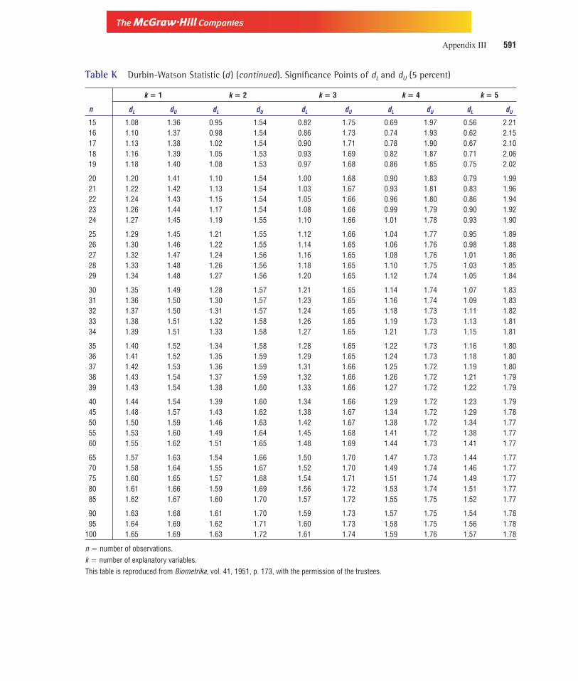
Version, Third Edition
Table K Durbin-Watson Statistic (d ) (continued). Significance Points of dL and dU (5 percent)
k � 1 k � 2 k � 3 k � 4 k � 5
n dL dU dL dU dL dU dL dU dL dU
15 1.08 1.36 0.95 1.54 0.82 1.75 0.69 1.97 0.56 2.2116 1.10 1.37 0.98 1.54 0.86 1.73 0.74 1.93 0.62 2.1517 1.13 1.38 1.02 1.54 0.90 1.71 0.78 1.90 0.67 2.1018 1.16 1.39 1.05 1.53 0.93 1.69 0.82 1.87 0.71 2.0619 1.18 1.40 1.08 1.53 0.97 1.68 0.86 1.85 0.75 2.02
20 1.20 1.41 1.10 1.54 1.00 1.68 0.90 1.83 0.79 1.9921 1.22 1.42 1.13 1.54 1.03 1.67 0.93 1.81 0.83 1.9622 1.24 1.43 1.15 1.54 1.05 1.66 0.96 1.80 0.86 1.9423 1.26 1.44 1.17 1.54 1.08 1.66 0.99 1.79 0.90 1.9224 1.27 1.45 1.19 1.55 1.10 1.66 1.01 1.78 0.93 1.90
25 1.29 1.45 1.21 1.55 1.12 1.66 1.04 1.77 0.95 1.8926 1.30 1.46 1.22 1.55 1.14 1.65 1.06 1.76 0.98 1.8827 1.32 1.47 1.24 1.56 1.16 1.65 1.08 1.76 1.01 1.8628 1.33 1.48 1.26 1.56 1.18 1.65 1.10 1.75 1.03 1.8529 1.34 1.48 1.27 1.56 1.20 1.65 1.12 1.74 1.05 1.84
30 1.35 1.49 1.28 1.57 1.21 1.65 1.14 1.74 1.07 1.8331 1.36 1.50 1.30 1.57 1.23 1.65 1.16 1.74 1.09 1.8332 1.37 1.50 1.31 1.57 1.24 1.65 1.18 1.73 1.11 1.8233 1.38 1.51 1.32 1.58 1.26 1.65 1.19 1.73 1.13 1.8134 1.39 1.51 1.33 1.58 1.27 1.65 1.21 1.73 1.15 1.81
35 1.40 1.52 1.34 1.58 1.28 1.65 1.22 1.73 1.16 1.8036 1.41 1.52 1.35 1.59 1.29 1.65 1.24 1.73 1.18 1.8037 1.42 1.53 1.36 1.59 1.31 1.66 1.25 1.72 1.19 1.8038 1.43 1.54 1.37 1.59 1.32 1.66 1.26 1.72 1.21 1.7939 1.43 1.54 1.38 1.60 1.33 1.66 1.27 1.72 1.22 1.79
40 1.44 1.54 1.39 1.60 1.34 1.66 1.29 1.72 1.23 1.7945 1.48 1.57 1.43 1.62 1.38 1.67 1.34 1.72 1.29 1.7850 1.50 1.59 1.46 1.63 1.42 1.67 1.38 1.72 1.34 1.7755 1.53 1.60 1.49 1.64 1.45 1.68 1.41 1.72 1.38 1.7760 1.55 1.62 1.51 1.65 1.48 1.69 1.44 1.73 1.41 1.77
65 1.57 1.63 1.54 1.66 1.50 1.70 1.47 1.73 1.44 1.7770 1.58 1.64 1.55 1.67 1.52 1.70 1.49 1.74 1.46 1.7775 1.60 1.65 1.57 1.68 1.54 1.71 1.51 1.74 1.49 1.7780 1.61 1.66 1.59 1.69 1.56 1.72 1.53 1.74 1.51 1.7785 1.62 1.67 1.60 1.70 1.57 1.72 1.55 1.75 1.52 1.77
90 1.63 1.68 1.61 1.70 1.59 1.73 1.57 1.75 1.54 1.7895 1.64 1.69 1.62 1.71 1.60 1.73 1.58 1.75 1.56 1.78
100 1.65 1.69 1.63 1.72 1.61 1.74 1.59 1.76 1.57 1.78
n � number of observations.k � number of explanatory variables.This table is reproduced from Biometrika, vol. 41, 1951, p. 173, with the permission of the trustees.
Appendix III 591

Version, Third Edition
Tabl
e L
Criti
cal V
alue
s of
the
Stu
dent
ized
Ran
ge D
istr
ibut
ion
for
a�
0.05 c
n�
c2
34
56
78
910
1112
1314
1516
1718
1920
118
.027
.032
.837
.140
.443
.145
.447
.449
.150
.652
.053
.254
.355
.456
.357
.258
.058
.859
.62
6.08
8.33
9.80
10.9
11.7
12.4
13.0
13.5
14.0
14.4
14.7
15.1
15.4
15.7
15.9
16.1
16.4
16.6
16.8
34.
505.
916.
827.
508.
048.
488.
859.
189.
469.
729.
9510
.210
.310
.510
.710
.811
.011
.111
.24
3.93
5.04
5.76
6.29
6.71
7.05
7.35
7.60
7.83
8.03
8.21
8.37
8.52
8.66
8.79
8.91
9.03
9.13
9.23
53.
644.
605.
225.
676.
036.
336.
586.
806.
997.
177.
327.
477.
607.
727.
837.
938.
038.
128.
216
3.46
4.34
4.90
5.30
5.63
5.90
6.12
6.32
6.49
6.65
6.79
6.92
7.03
7.14
7.24
7.34
7.43
7.51
7.59
73.
344.
164.
685.
065.
365.
615.
826.
006.
166.
306.
436.
556.
666.
766.
856.
947.
027.
107.
178
3.26
4.04
4.53
4.89
5.17
5.40
5.60
5.77
5.92
6.05
6.18
6.29
6.39
6.48
6.57
6.65
6.73
6.80
6.87
93.
203.
954.
414.
765.
025.
245.
435.
595.
745.
875.
986.
096.
196.
286.
366.
446.
516.
586.
64
103.
153.
884.
334.
654.
915.
125.
305.
465.
605.
725.
835.
936.
036.
116.
196.
276.
346.
406.
4711
3.11
3.82
4.26
4.57
4.82
5.03
5.20
5.35
5.49
5.61
5.71
5.81
5.90
5.98
6.06
6.13
6.20
6.27
6.33
123.
083.
774.
204.
514.
754.
955.
125.
275.
395.
515.
615.
715.
805.
885.
956.
026.
096.
156.
2113
3.06
3.73
4.15
4.45
4.69
4.88
5.05
5.19
5.32
5.43
5.53
5.63
5.71
5.79
5.86
5.93
5.99
6.05
6.11
143.
033.
704.
114.
414.
644.
834.
995.
135.
255.
365.
465.
555.
645.
715.
795.
855.
915.
976.
03
153.
013.
674.
084.
374.
594.
784.
945.
085.
205.
315.
405.
495.
575.
655.
725.
785.
855.
905.
9616
3.00
3.65
4.05
4.33
4.56
4.74
4.90
5.03
5.15
5.26
5.35
5.44
5.52
5.59
5.66
5.73
5.79
5.84
5.90
172.
983.
634.
024.
304.
524.
704.
864.
995.
115.
215.
315.
395.
475.
545.
615.
675.
735.
795.
8418
2.97
3.61
4.00
4.28
4.49
4.67
4.82
4.96
5.07
5.17
5.27
5.35
5.43
5.50
5.57
5.63
5.69
5.74
5.79
192.
963.
593.
984.
254.
474.
654.
794.
925.
045.
145.
235.
315.
395.
465.
535.
595.
655.
705.
75
202.
953.
583.
964.
234.
454.
624.
774.
905.
015.
115.
205.
285.
365.
435.
495.
555.
615.
665.
7124
2.92
3.53
3.90
4.17
4.37
4.54
4.68
4.81
4.92
5.01
5.10
5.18
5.25
5.32
5.38
5.44
5.49
5.55
5.59
302.
893.
493.
854.
104.
304.
464.
604.
724.
824.
925.
005.
085.
155.
215.
275.
335.
385.
435.
4740
2.86
3.44
3.79
4.04
4.23
4.39
4.52
4.63
4.73
4.82
4.90
4.98
5.04
5.11
5.16
5.22
5.27
5.31
5.36
602.
833.
403.
743.
984.
164.
314.
444.
554.
654.
734.
814.
884.
945.
005.
065.
115.
155.
205.
2412
02.
803.
363.
683.
924.
104.
244.
364.
474.
564.
644.
714.
784.
844.
904.
955.
005.
045.
095.
13a
2.77
3.31
3.63
3.86
4.03
4.17
4.29
4.39
4.47
4.55
4.62
4.68
4.74
4.80
4.85
4.89
4.93
4.97
5.01
Sour
ce: R
eprin
ted
by p
erm
issi
on o
f the
Bio
met
rika
trust
ees
from
E. S
. Pea
rson
and
H. O
. Har
tley,
eds
., Bi
omet
rika
Tabl
es fo
r Sta
tistic
ians
,vol
. 1, 3
rd e
d. (C
ambr
idge
Uni
vers
ity P
ress
, 196
6).
592

Version, Third Edition
Tabl
e L
Criti
cal V
alue
s of
the
Stu
dent
ized
Ran
ge D
istr
ibut
ion
for
a�
0.01
(con
clud
ed)
cn
�c
23
45
67
89
1011
1213
1415
1617
1819
20
190
.013
516
418
620
221
622
723
724
625
326
026
627
227
728
228
629
029
429
82
14.0
19.0
22.3
24.7
26.6
28.2
29.5
30.7
31.7
32.6
33.4
34.1
34.8
35.4
36.0
36.5
37.0
37.5
37.9
38.
2610
.612
.213
.314
.215
.015
.616
.216
.717
.117
.517
.918
.218
.518
.819
.119
.319
.519
.84
6.51
8.12
9.17
9.96
10.6
11.1
11.5
11.9
12.3
12.6
12.8
13.1
13.3
13.5
13.7
13.9
14.1
14.2
14.4
55.
706.
977.
808.
428.
919.
329.
679.
9710
.210
.510
.710
.911
.111
.211
.411
.611
.711
.811
.96
5.24
6.33
7.03
7.56
7.97
8.32
8.61
8.87
9.10
9.30
9.49
9.65
9.81
9.95
10.1
10.2
10.3
10.4
10.5
74.
955.
926.
547.
017.
377.
687.
948.
178.
378.
558.
718.
869.
009.
129.
249.
359.
469.
559.
658
4.74
5.63
6.20
6.63
6.96
7.24
7.47
7.68
7.87
8.03
8.18
8.31
8.44
8.55
8.66
8.76
8.85
8.94
9.03
94.
605.
435.
966.
356.
666.
917.
137.
327.
497.
657.
787.
918.
038.
138.
238.
328.
418.
498.
57
104.
485.
275.
776.
146.
436.
676.
877.
057.
217.
367.
487.
607.
717.
817.
917.
998.
078.
158.
2211
4.39
5.14
5.62
5.97
6.25
6.48
6.67
6.84
6.99
7.13
7.25
7.36
7.46
7.56
7.65
7.73
7.81
7.88
7.95
124.
325.
045.
505.
846.
106.
326.
516.
676.
816.
947.
067.
177.
267.
367.
447.
527.
597.
667.
73
134.
264.
965.
405.
735.
986.
196.
376.
536.
676.
796.
907.
017.
107.
197.
277.
347.
427.
487.
55
144.
214.
895.
325.
635.
886.
086.
266.
416.
546.
666.
776.
876.
967.
057.
127.
207.
277.
337.
39
154.
174.
835.
255.
565.
805.
996.
166.
316.
446.
556.
666.
766.
846.
937.
007.
077.
147.
207.
2616
4.13
4.78
5.19
5.49
5.72
5.92
6.08
6.22
6.35
6.46
6.56
6.66
6.74
6.82
6.90
6.97
7.03
7.09
7.15
174.
104.
745.
145.
435.
665.
856.
016.
156.
276.
386.
486.
576.
666.
736.
806.
876.
947.
007.
0518
4.07
4.70
5.09
5.38
5.60
5.79
5.94
6.08
6.20
6.31
6.41
6.50
6.58
6.65
6.72
6.79
6.85
6.91
6.96
194.
054.
675.
055.
335.
555.
735.
896.
026.
146.
256.
346.
436.
516.
586.
656.
726.
786.
846.
89
204.
024.
645.
025.
295.
515.
695.
845.
976.
096.
196.
296.
376.
456.
526.
596.
656.
716.
766.
8224
3.96
4.54
4.91
5.17
5.37
5.54
5.69
5.81
5.92
6.02
6.11
6.19
6.26
6.33
6.39
6.45
6.51
6.56
6.61
303.
894.
454.
805.
055.
245.
405.
545.
655.
765.
855.
936.
016.
086.
146.
206.
266.
316.
366.
4140
3.82
4.37
4.70
4.93
5.11
5.27
5.39
5.50
5.60
5.69
5.77
5.84
5.90
5.96
6.02
6.07
6.12
6.17
6.21
603.
764.
284.
604.
824.
995.
135.
255.
365.
455.
535.
605.
675.
735.
795.
845.
895.
935.
986.
0212
03.
704.
204.
504.
714.
875.
015.
125.
215.
305.
385.
445.
515.
565.
615.
665.
715.
755.
795.
83a
3.64
4.12
4.40
4.60
4.76
4.88
4.99
5.08
5.16
5.23
5.29
5.35
5.40
5.45
5.49
5.54
5.57
5.61
5.65
Sour
ce: R
eprin
ted
by p
erm
issi
on o
f the
Bio
met
rika
trust
ees
from
E. S
. Pea
rson
and
H. O
. Har
tley,
eds
., Bi
omet
rika
Tabl
es fo
r Sta
tistic
ians
,vol
. 1, 3
rd e
d. (C
ambr
idge
Uni
vers
ity P
ress
, 196
6).
593

Version, Third Edition
Table M Critical Values of r in the Runs Test
Table M1 and Table M2 contain various critical values of r for various values of n1 and n2. For the one-sample runstest, any value of r that is equal to or smaller than that shown in Table M1 or equal to or larger than that shown inTable M2 is significant at the 0.05 level.
Table M1
n22 3 4 5 6 7 8 9 10 11 12 13 14 15 16 17 18 19 20n1
2 2 2 2 2 2 2 2 2 23 2 2 2 2 2 2 2 2 2 3 3 3 3 3 34 2 2 2 3 3 3 3 3 3 3 3 4 4 4 4 45 2 2 3 3 3 3 3 4 4 4 4 4 4 4 5 5 56 2 2 3 3 3 3 4 4 4 4 5 5 5 5 5 5 6 67 2 2 3 3 3 4 4 5 5 5 5 5 6 6 6 6 6 68 2 3 3 3 4 4 5 5 5 6 6 6 6 6 7 7 7 79 2 3 3 4 4 5 5 5 6 6 6 7 7 7 7 8 8 810 2 3 3 4 5 5 5 6 6 7 7 7 7 8 8 8 8 911 2 3 4 4 5 5 6 6 7 7 7 8 8 8 9 9 9 912 2 2 3 4 4 5 6 6 7 7 7 8 8 8 9 9 9 10 1013 2 2 3 4 5 5 6 6 7 7 8 8 9 9 9 10 10 10 1014 2 2 3 4 5 5 6 7 7 8 8 9 9 9 10 10 10 11 1115 2 3 3 4 5 6 6 7 7 8 8 9 9 10 10 11 11 11 1216 2 3 4 4 5 6 6 7 8 8 9 9 10 10 11 11 11 12 1217 2 3 4 4 5 6 7 7 8 9 9 10 10 11 11 11 12 12 1318 2 3 4 5 5 6 7 8 8 9 9 10 10 11 11 12 12 13 1319 2 3 4 5 6 6 7 8 8 9 10 10 11 11 12 12 13 13 1320 2 3 4 5 6 6 7 8 9 9 10 10 11 12 12 13 13 13 14
Table M2
n22 3 4 5 6 7 8 9 10 11 12 13 14 15 16 17 18 19 20n1
234 9 95 9 10 10 11 11
6 9 10 11 12 12 13 13 13 137 11 12 13 13 14 14 14 14 15 15 158 11 12 13 14 14 15 15 16 16 16 16 17 17 17 17 179 13 14 14 15 16 16 16 17 17 18 18 18 18 18 18
10 13 14 15 16 16 17 17 18 18 18 19 19 19 20 2011 13 14 15 16 17 17 18 19 19 19 20 20 20 21 2112 13 14 16 16 17 18 19 19 20 20 21 21 21 22 2213 15 16 17 18 19 19 20 20 21 21 22 22 23 2314 15 16 17 18 19 20 20 21 22 22 23 23 23 24
15 15 16 18 18 19 20 21 22 22 23 23 24 24 2516 17 18 19 20 21 21 22 23 23 24 25 25 2517 17 18 19 20 21 22 23 23 24 25 25 26 2618 17 18 19 20 21 22 23 24 25 25 26 26 2719 17 18 20 21 22 23 23 24 25 26 26 27 2720 17 18 20 21 22 23 24 25 25 26 27 27 28
Source: Adapted from Frieda S. Swed and C. Eisenhart, “Tables for Testing Randomness of Grouping in a Sequenceof Alternatives,” Annals of Mathematical Statistics 14, 1943, pp. 66–87. Used by permission.
594 Statistical Tables

Version, Third Edition
Table N Spearman’s Rank Correlation, Combined Areas in Both Tails
Example: For a two-tailed test of significance at the 0.20 level, with n � 10, the appropriate value for r can be foundby looking under the 0.20 column and proceeding down to the 10; there we find the appropriate rs value to be 0.4424.
n 0.20 0.10 0.05 0.02 0.01 0.002
4 0.8000 0.80005 0.7000 0.8000 0.9000 0.9000
6 0.6000 0.7714 0.8286 0.8857 0.94297 0.5357 0.6786 0.7450 0.8571 0.8929 0.96438 0.5000 0.6190 0.7143 0.8095 0.8571 0.92869 0.4667 0.5833 0.6833 0.7667 0.8167 0.900010 0.4424 0.5515 0.6364 0.7333 0.7818 0.8667
11 0.4182 0.5273 0.6091 0.7000 0.7455 0.836412 0.3986 0.4965 0.5804 0.6713 0.7273 0.818213 0.3791 0.4780 0.5549 0.6429 0.6978 0.791214 0.3626 0.4593 0.5341 0.6220 0.6747 0.767015 0.3500 0.4429 0.5179 0.6000 0.6536 0.7464
16 0.3382 0.4265 0.5000 0.5824 0.6324 0.726517 0.3260 0.4118 0.4853 0.5637 0.6152 0.708318 0.3148 0.3994 0.4716 0.5480 0.5975 0.690419 0.3070 0.3895 0.4579 0.5333 0.5825 0.673720 0.2977 0.3789 0.4451 0.5203 0.5684 0.6586
21 0.2909 0.3688 0.4351 0.5078 0.5545 0.645522 0.2829 0.3597 0.4241 0.4963 0.5426 0.631823 0.2767 0.3518 0.4150 0.4852 0.5306 0.618624 0.2704 0.3435 0.4061 0.4748 0.5200 0.607025 0.2646 0.3362 0.3977 0.4654 0.5100 0.5962
26 0.2588 0.3299 0.3894 0.4564 0.5002 0.585627 0.2540 0.3236 0.3822 0.4481 0.4915 0.575728 0.2490 0.3175 0.3749 0.4401 0.4828 0.566029 0.2443 0.3113 0.3685 0.4320 0.4744 0.556730 0.2400 0.3059 0.3620 0.4251 0.4665 0.5479
Source: Adapted from Glasser and Winter, Biometrika, 1961, with the permission of the Biometrika trustees.
Appendix III 595
– 0.4424
0.10 of area
0.4424
0.10 of area
(n = sample size = 10)

Version, Third Edition
Table O Critical Factors for Control Charts
Chart for Averages Chart for Ranges
Factor for Factor for Factors forControl Limit Central Line Control Limits
n A2 d2 D3 D4 d3
2 1.880 1.128 0 3.267 0.85253 1.023 1.693 0 2.575 0.88844 0.729 2.059 0 2.282 0.87985 0.577 2.326 0 2.115 0.8641
6 0.483 2.534 0 2.004 0.84807 0.419 2.704 0.076 1.924 0.8338 0.373 2.847 0.136 1.864 0.8209 0.337 2.970 0.184 1.816 0.80810 0.308 3.078 0.223 1.777 0.797
11 0.285 3.173 0.256 1.744 0.78712 0.266 3.258 0.284 1.716 0.77813 0.249 3.336 0.308 1.692 0.77014 0.235 3.407 0.329 1.671 0.76215 0.223 3.472 0.348 1.652 0.755
16 0.212 3.532 0.364 1.636 0.74917 0.203 3.588 0.379 1.621 0.74318 0.194 3.640 0.392 1.608 0.73819 0.187 3.689 0.404 1.596 0.73320 0.180 3.735 0.414 1.586 0.729
21 0.173 3.778 0.425 1.575 0.72422 0.167 3.819 0.434 1.566 0.72023 0.162 3.858 0.443 1.557 0.71624 0.157 3.895 0.452 1.548 0.71225 0.153 3.931 0.459 1.541 0.709
Source: Values of d2 and d3 are from E. S. Pearson, “The Percentage Limits for the Distribution of Range in Samplesfrom a Normal Population,” Biometrika 24, 1932, p. 416. Used by permission of the Biometrika trustees.A2 � 3�(d2 �n�), D3 � 1 � 3(d3�d2), D4 � 1 � 3(d3�d2).
596 Statistical Tables

Version, Third Edition
Table P Combinatorials
n nC0 nC1 nC2 nC3 nC4 nC5 nC6 nC7 nC8 nC9 nC10
0 11 1 12 1 2 13 1 3 3 14 1 4 6 4 1
5 1 5 10 10 5 16 1 6 15 20 15 6 17 1 7 21 35 35 21 7 18 1 8 28 56 70 56 28 8 19 1 9 36 84 126 126 84 36 9 1
10 1 10 45 120 210 252 210 120 45 10 111 1 11 55 165 330 462 462 330 165 55 1112 1 12 66 220 495 792 924 792 495 220 6613 1 13 78 286 715 1287 1716 1716 1287 715 28614 1 14 91 364 1001 2002 3003 3432 3003 2002 1001
15 1 15 105 455 1365 3003 5005 6435 6435 5005 300316 1 16 120 560 1820 4368 8008 11440 12870 11440 800817 1 17 136 680 2380 6188 12376 19448 24310 24310 1944818 1 18 153 816 3060 8568 18564 31824 43758 48620 4375819 1 19 171 969 3876 11628 27132 50388 75582 92378 92378
20 1 20 190 1140 4845 15504 38760 77520 125970 167960 184756
Appendix III 597

Version, Third Edition
AAcceptance number, 521Acceptance quality level (AQL), 8, 520Acceptance sampling, 8, 520–523Accuracy, 10–11Addition rule of probability, 87–89Adjusted coefficient of determination, 370Alpha-value, 171–172, 196, 197, 249Alternative hypothesis, 195; see also Null hypothesisAnalysis of variance (ANOVA), 266–268; see also
One-way ANOVA; Two-way ANOVAF-ratio, 270multiple regression model, 371–372for regression model, 348–349table, 274–277test for balanced design, 277–280test for unbalanced design, 280–283
Arithmetic mean, 41; see also MeanAssignable cause variation, 501Attribute control charts
c-charts, 515–518p-charts, 511–515
Autocorrelation, 330–331Averages, 40–41
BBalanced designs, tests for; see also Unbalanced designs
least significant difference approach, 278–280Tukey’s criterion, 278
Bayes, Rev. Thomas, 89Bayes Theorem, 89–92Bell-shaped symmetrical curve, 60Bernoulli, Jacob, 106Bernoulli process, 106Beta coefficients; see Standardized regression coefficientsBetween-sample variation, 269Bias, sampling, 11, 158Bimodal data set, 42Binomial distributions, 132
calculating, 107–108cumulative, 109–110defined, 106mean, 108normal approximation to, 130–131, 135properties of, 106using computer for, 110–111variance, 109
Bivariate regression; see Simple regressionBlocking, 283–286Blocking design, 293Business report writing, 535–540
CC. I.; see Confidence interval (C. I.)Causation, 339C-charts, 515–518Cells, 25Central Limit Theorem, 148–149Central tendency; see Measures of central tendencyChance variation, 501Chebyshev, P. L., 59Chebyshev’s Theorem, 59Chi-square (X2) distribution
goodness-of-fit tests, 447–454tests for independence, 454–459
Class(es), c, 21–24boundaries, 22determining number of, 22interval, 22–23midpoint, M, 22rule for determining number of, 22
Classical approach to probability, 78Cluster sampling, 160Coefficient of determination, 338–339Coefficient of multiple determination, 369–370Coefficient of skewness, 62Coefficient of variation (CV), 63Collective exhaustive events, 81Combinations, 92–93Complementary events, 82Completely randomized design, 293; see also One-way
ANOVAComposite price index, 423–424Computers; see Excel; MinitabConditional mean, 343–345Conditional probability, 84–85, 90–91Confidence coefficient, 169, 170Confidence interval (C. I.), 168–169
of the conditional mean, 344controlling width of, 179–180for difference between two proportions, 238–240interpretation, 171–172of population mean
large samples, 170–174small sample, 174–177
for population proportions, 177–178for the predictive interval, 346principle of, 169–170when population standard deviation is known, 172–173
Consistent estimator, 185Constraints, 51Consumer Price Index (CPI), 429–432Consumer risk, 521
598
I n d e x

Version, Third Edition
Index 599
Contingency tables, 24–25, 454–459for probability of events, 82–86
Continuity correction factor, 131Continuous random variable, 103Continuous variable, 10Control charts, 499
for attributesc-charts, 515–518p-charts, 511–515
interpreting, 518–519for variables, 501–504
R-chart, 507–510X�-chart, 504–507
Conversion formula; see Z formulaCorrelation, causation and, 339–340Correlation analysis, 336–339Correlation coefficient (r), 336–338Counting techniques, 92–94Critical values, for Z and rejection regions, 196–197Cumulative binomial distributions, 109–110Curvilinear regression
defined, 317–318logarithmic models, 389–391polynomial models, 388–389
Cyclical fluctuations, 401Cyclical variation, 419–420
DData, methods of organizing, 20–21; see also Grouped dataDeasonalized values, 416Deciles, 57–58Decision rule, 197Deflating, a time series, 431Degrees of freedom, 51
for unequal population variances, 232–233Deming, W. Edward, 499–501Dependent events, probability of, 86Dependent variable, 316–317Depths, 29Descriptive statistics, 10Deterministic relationships, 319Deviation, measures of, 337–338Discrete distributions, 104–106Discrete random variable, 103Discrete variable, 10Dispersion; see Measures of dispersionDistribution
binomial, 106–111discrete, 104–106exponential, 116–118hypergeometric, 111–113normal, 121–131Poisson, 113–116sampling, 143–148
Distribution—Cont.uniform, 118–121
Distribution-free tests; see Nonparametric testsDow Jones industrial average, 430Dummy variables, 383–387Durbin-Watson test, 331
EEconomic analysts, 6Education Industry Report, 4Efficient estimator, 18580/20 rule, 7Empirical Rule, 60–62, 121–123, 169, 334Error
level of significance and, 197tolerable, 180Type I, 197Type II, 197
Error mean square (MSE), 273Error sum of squares (SSE), 271–272Estimates, 168–169
defined, 183–184Estimators
defined, 183–184properties of good, 184–186
Events, 80–82Excel
for binomial distributions, 110–111exponential distribution, 117–118for hypergeometric distributions, 113Poisson distribution, 115–116
Executive summary, 536, 537–538Expected frequencies, 450–451Expected value E(X), for probability distribution, 104Experiment, defined, 77Experimental units, 267Explained deviation, 337Exponential distribution, 116–117, 133
using the computer, 117–118Exponential smoothing, 406–409
FFactorial analysis, 292–296Failure, probability of (1 � �), 106F-distribution, 248–250Financial analysts, 6Finite population correction factor (fpc), 147Fisher, Sir Ronald A., 248Fixed-effects model, 267Fluctuations, 400–401F-ratio, 249
as used in ANOVA, 270Frequency distribution, 21–24
less-than cumulative, 23–24

Version, Third Edition
Index 600
Frequency distribution—Cont.more-than cumulative, 23relative, 23–24
GGalton, Sir Francis, 317Geometric mean, 44–46Goodness-of-fit; see also Standard error of the estimate
for chi-square (X2), 447–454coefficient of multiple determination, 369–370
Grand mean, 144–145, 269Gross national product (GNP), 431Grouped data
mean, 53–54median, 54mode, 54–55variance and standard deviation for, 55–56
Gusset, William S., 174
HHeteroscedasticity, 329High-low close chart, 28–29Histogram, 27–28Homoscedasticity, 328–329Hypergeometric distribution, 111–113, 132Hyperplane, 366Hypothesis
alternative, 195null, 195
Hypothesis testingprinciple of, 195–197probability of error in, 197rejection regions in, 196–197steps in, 198
Hypothesis testsfor differences in proportions, 247–248with paired data, 245–246two means with independent sampling
large samples, 241–244small sample estimation, 244–245
IIndependent events, 81–82
joint probability of, 85–86Independent samples, for two-population tests, 227Independent sampling
large sample estimation, 227–230small sample estimation, 230–234
Independent variable, 316–317Index number
composite price, 423–424simple price, 421–423weighted composite price
Laspeyres, 424–429Paasche, 426–429
Industrial production index, 430Inferential statistics, 10, 142–143Interaction, 294–295Internet, career information on, 16–17Intersection, 80Interval
factors influencing width of, 347–348Interval estimation, 168–169confidence interval for differences between two propor-
tions, 238–240independent sampling
large sample, 227–230small sample, 230–234
paired sampling, 234–238in regression analysis, 343–348
Interval measurements, 13, 14Irregular fluctuations, 401Irregular variation, 420–421
JJoint events, 80
determining probability of, 85–87Joint probabilities, 83Juran, Joseph, 501
KKruskal-Wallis test, 476–480
LLaspeyres index, 424–429Latin square design, 296–298LCL; see Lower confidence limit (LCL)Leaf unit, 29Least significant difference (LSD)
for balanced designs, 277–280for unbalanced designs, 280–283
Less-than cumulative frequency distribution, 23–24Level of significance, 196
probability error and, 197Linear regression
assumptions of, 328–332defined, 317–318determining model, 318–320ordinary least squares (OLS) model, 320–323standard error of the estimate, 332–336
Line of best fit, 322Logarithmic models of curvilinear regression, 389–391Lower confidence limit (LCL), 169
MMain-effects test, 293Malcolm Baldrige National Quality Award, 500–501

Version, Third Edition
Index 601
Mann-Whitney U-Test, 467–472, 480Marginal probabilities, 83Mean; see also Population mean; Sample mean
binomial distributions, 108compared to median and mode, 46–47confidence interval of population, 170–173geometric, 44–46grouped, 53–54one-tailed test for, 201–203of probability distribution, 104of the sample means, 144–145sample size for, 181selecting proper test statistic for, 176small sample intervals for, 174–176small-sample tests for, 209–211two-tailed test for, 198–199weighted, 43–44
Mean ratio to moving average, 415Mean square error (MSE), 273Mean square treatment (MSTR), 273Mean sums of squares, 272–274Measurement, levels of
interval, 13nominal, 12–13ordinal, 13ratio, 14
Measures of central tendency, 40–41comparing, 46–47geometric mean, 44–46for grouped data, 53–55mean, 41media, 42mode, 42–43weighted mean, 43
Measures of dispersion, 41, 47–48, 57–58defined, 46–47for grouped data, 55–57range, 48relative, 63standard deviation, 48–50variance, 48–50
Median, 42compared to mean and mode, 46–47for grouped data, 54
Minitabfor binomial distributions, 110–111confidence intervals, 172–173Poisson distribution, 115–116p-value, 207two-tailed test for mu, 199uniform distribution, 120–121
Mode, 42–43compared to median and mean, 46–47for grouped data, 54–55
More-than cumulative frequency distribution, 23Moving average (MA), 403–406Multicollinearity, 365, 377–381Multiple-choice counting method, 94Multiple regression, 317
adjusted coefficient of determination, 370coefficient of multiple determination, 369–370model, 365–366standard error of the estimate, 367–369tests of significance, 371–374
Multiple sampling plans, 522Multiplication rule of probability, 85–87Mutual Fund Investor’s Center, 73Mutually exclusive events, 81
NNegative autocorrelation, 330–331Net regression coefficients, 365Nominal measurements, 12–13Nonparametric tests, 446–447
chi-square distribution, 447–459compared to parametric tests, 480Kruskal-Wallis test, 476–480Mann-Whitney U Test, 467–472runs test, 463–467sign test, 459–463Spearman rank correlation, 472–476
Normal approximation, to binomial distribution, 130–131,135
Normal deviate, 123–124, 181calculating probabilities with, 124–128for sampling distribution for proportions, 156
Normal distribution, 59–62, 121–124, 133–134Normalization ratio, 415–416Normal populations
comparing the variance of two, 248–250Null hypothesis, 195
OOne-tailed test
Mann-Whitney U Test, 470–471for mu ( ), 201–203
One-way ANOVAdefined, 268–269principles, 269–270
Operating characteristic (OC) curves, 522–523Ordered array, 21, 29Ordinal measurements, 13Ordinary least squares (OLS), 320–323
runs test application, 465–467Outcome, 77Outliers, 46

Version, Third Edition
Index 602
PPaasche index, 426–429Pair comparison
least significant difference (LSD), 277–280Tukey’s criterion, 277–278
Paired samples, 234–238hypotheses tests with, 245–246for two-population tests, 227
Parameter, 9Parametric tests, 446
compared to nonparametric tests, 480Pareto, Vilfrado, 7Pareto chart, 7Partial regression coefficients, 365
testing individual, 372–374Patterns, detection of, 464P-charts, 511–515Pearson, Karl, 336Pearsonian coefficient of skewness, 62Pearsonian product-moment correlation coefficient,
336Percentage point increase, 422Percentiles, 57–58Permutations, 92–93Pictorial displays; see specific methodPie charts, 28Point estimate, 168–169Poisson, Simeon, 113Poisson distribution, 113–116, 133
using computer for, 115–116Polynomial models of curvilinear regression, 388–389Pooled estimate, 230Population, 142; see also Mean
defined, 8–9standard deviation, 48–50variance, 48–50
Population correlation coefficient, tests for, 342–343Population mean, 41Population parameters, tests for, 340–343Population proportion, 177–178
tests for, 212–214Positional average; see MedianPositive autocorrelation, 330–331Predictive interval, 343
for a single value of Y, 345–348Probability, 76–77
addition rule for, 87–89classical approach, 78–79conditional, 84–85multiplication rule for, 85–87relative frequency approach, 77–78subjective approach, 78
Probability distribution, 103–104mean of, 104
Probability distribution—Cont.standard deviation of, 105variance of, 104–105
Probability of failure, 106Probability of success, 106Probability tables, for events, 82–83Produce price index, 430Producer risk, 520Product improvement; see Quality control (QC)p-value
defined, 206–207two-tailed tests and, 207–208
QQualitative variable, 10, 384Quality control (QC), 7
history of, 499–501Quality control (QC) circles, 7Quality function deployment (QFD), 7Quantitative variable, 10Quartiles, 57–58
RRandom-effects model, 267Random fluctuation, 401Randomized block design, 283–292Randomness, 463–465Random variable, 102–103
continuous, 103discrete, 103
Random walk exhibits, 399Range, 48Ratio measurements, 14Rational subgrouping, 502Ratio to moving average, 415R-chart, 507–510Real gross national product (GNP), 432Real income, 431Regression analysis, 317–318; see also Multiple regression
interval estimation in, 343–348limitations of, 339–350ordinary least squares (OLS), 320–323simple linear model, 318–320standard error of the estimate, 332–335
Regression coefficient, 322–323comparing, 381–382
Regression plane, 366Relative frequency, 77–78Relative frequency distribution, 23–24Report writing, 535–540Rules of probability
addition, 87–89multiplication, 85–87
Run, 463Runs test, 463–467, 480

Version, Third Edition
Index 603
SSample, 10, 142
defined, 9standard deviation s, 50–52variance, 50–52
Sample mean (X-bar), 41Sample size
determining proper, 180–182increasing, 180for population estimate (π), 182selecting proper, 240–241
Sample space (SS), 77Sample standard deviation, for grouped data, 55–56Sample variance, 271
for grouped data, 55–56Sampling
cluster, 160with replacement, 147simple random sample, 158–159stratified, 159systematic, 159
Sampling bias, 11, 158Sampling distribution, 150–151, 169
defined, 143–144for proportions, 155–158
expect value, 155–156standard error, 156
for sample means, 144–145applications, 150–154Central Limit Theorem, 148–149mean, 144–145standard error, 145–147variance, 145–147
Sampling error, 143causes of, 11defined, 11sources, 158
Sampling methods, 158–161cluster, 160simple random, 158–159stratified, 159systematic, 159
Sampling plans, 522Scatter diagrams, 317–318Seasonal fluctuations, 400Seasonal variation, 413–419Secular trend, 400Sequential sampling plans, 522Set, 80Shewhart, Walter, 501Sign test, 459–463, 480Simple price index, 420–423Simple random sample, 158–159Simple regression, 317Skewness, 62
Small-sample tests, mean and, 209–211Smoothing techniques
exponential, 406–409moving average, 403–406
Spearman rank correlation, 472–476, 480Specification bias, 381Spurious correlation, 340Standard deviation
common uses for, 59–64confidence intervals and, 172–173population, 48–50of probability distributions, 105sample s, 50–52
Standard errorof the conditional mean, 344for difference in two sample proportions, 238–239of the forecast, 346impact of sample size on, 147for sample means, 145–147using finite population correction factor (fpc), 147
Standard error of the estimate (Se), 332–336for multiple regression, 367–369
Standardized regression coefficients, 382Standard normal distribution, 123Standard & Poor’s composite index, 430Statistical literacy, need for, 8Statistically insignificant difference, 195–196Statistical norm, in cyclical variation, 419–420Statistical quality control (SQC), 7, 8Statistics
career opportunities in, 6–8defined, 9descriptive, 10function of, 11–12importance of, 4–5inferential, 10universal application of, 6
Stem-and-leaf design, 29Stepwise regression, 383Stochastic relationships, 319Stratified sampling, 159Student’s t distribution, 174–176Subgroup, 501–503Subjective approach to probability, 78Success, probability of (π), 106Sufficient estimator, 185–186Sum of squared errors, 321–322Sum of the squares of the row block (SSRB), 297–298Sums of squares, 270–272Systematic sampling, 159
Tt-distribution, 230–234, 244–245; see also Student’s
t-distribution

Version, Third Edition
Index 604
Ticks and tabs, 29Time series
components, 399–401decomposition of
irregular variation, 420–421isolating cyclical variation, 419–420isolating seasonal component, 413–419
models, 402smoothing techniques, 402–409trend analysis, 410–413
Tolerable error, 180Total deviation, 337Total mean squares (MST), 272–273Total quality management (TQM), 7–8Total variation, 269, 270Tradeline Mutual Fund Center, 73Treatment, 266–267, 293Treatment effect, 270Treatment sum of squares, 271Tree diagram, 90Trend analysis, 410–413Tukey, J., 29Tukey’s criterion (T), 277–278Two populations, 226–227Two-population tests
independent samples, 227–233paired samples, 227, 234–238
Two-tailed tests, 198–199Mann-Whitney U Test, 470p-value for, 207–208
Two-way (ANOVA); see also Analysis of variance(ANOVA)
randomized block design, 283–292Type I error, 197
acceptance sampling, 520Type II error, 197
acceptance sampling, 521
UUCL; see Upper confidence limit (UCL)Unbalanced designs; see also Balanced designs, tests for
alternate LSD approach, 280–283Unbiased estimator (theta), 184Unequal population variances, degrees of freedom for,
232–233Unexplained deviation, 337–338Uniform distribution, 133Uniform probability distribution, 118–121
using computer for, 120–121Union events, 80–81Universe; see PopulationUpper confidence limit (UCL), 169U Test; See Mann-Whitney U-Test
VVariable
continuous, 10defined, 9–10discrete, 10interval, 13nominal, 12–13ordinal, 13qualitative, 10quantitative, 10random, 102–103ratio, 14
Variable control chartsR-charts, 507–510X�, 504–507
Variancebinomial distributions, 109comparing, of two normal populations, 248–250population, 48–50of probability distribution, 104–105problems, 49sample, 50–52for sample means, 145–147
Variance inflation factor (VIF), 379Variation, 269Venn, John, 80Venn diagram, 80VIF; See Variance inflation factor (VIF)
WWalter Shewhart, 499Weighted composite price index
Laspeyres, 424–429Paasche, 426–429
Weighted mean, 43–44Within-sample variation, 269
X
X�-chart, 504–507X-values
calculating, from a known probability, 128–130
ZZ-distribution, 174Z-formula, 123–124, 150Z (test), 212–214Z-test statistic
for large samples, 241–242Z-value, 123–124, 169, 196–197
calculating X-values from known, 128–130

Version, Third Edition
Table E The Normal Distribution
Z 0.00 0.01 0.02 0.03 0.04 0.05 0.06 0.07 0.08 0.09
0.0 0.0000 0.0040 0.0080 0.0120 0.0160 0.0199 0.0239 0.0279 0.0319 0.03590.1 0.0398 0.0438 0.0478 0.0517 0.0557 0.0596 0.0636 0.0675 0.0714 0.07530.2 0.0793 0.0832 0.0871 0.0910 0.0948 0.0987 0.1026 0.1064 0.1103 0.11410.3 0.1179 0.1217 0.1255 0.1293 0.1331 0.1368 0.1406 0.1443 0.1480 0.15170.4 0.1554 0.1591 0.1628 0.1664 0.1700 0.1736 0.1772 0.1808 0.1844 0.1879
0.5 0.1915 0.1950 0.1985 0.2019 0.2054 0.2088 0.2123 0.2157 0.2190 0.22240.6 0.2257 0.2291 0.2324 0.2357 0.2389 0.2422 0.2454 0.2486 0.2517 0.25490.7 0.2580 0.2611 0.2642 0.2673 0.2704 0.2734 0.2764 0.2794 0.2823 0.28520.8 0.2881 0.2910 0.2939 0.2967 0.2995 0.3023 0.3051 0.3078 0.3106 0.31330.9 0.3159 0.3186 0.3212 0.3238 0.3264 0.3289 0.3315 0.3340 0.3365 0.3389
1.0 0.3413 0.3438 0.3461 0.3485 0.3508 0.3531 0.3554 0.3577 0.3599 0.36211.1 0.3643 0.3665 0.3686 0.3708 0.3729 0.3749 0.3770 0.3790 0.3810 0.38301.2 0.3849 0.3869 0.3888 0.3907 0.3925 0.3944 0.3962 0.3980 0.3997 0.40151.3 0.4032 0.4049 0.4066 0.4082 0.4099 0.4115 0.4131 0.4147 0.4162 0.41771.4 0.4192 0.4207 0.4222 0.4236 0.4251 0.4265 0.4279 0.4292 0.4306 0.4319
1.5 0.4332 0.4345 0.4357 0.4370 0.4382 0.4394 0.4406 0.4418 0.4429 0.44411.6 0.4452 0.4463 0.4474 0.4484 0.4495 0.4505 0.4515 0.4525 0.4535 0.45451.7 0.4554 0.4564 0.4573 0.4582 0.4591 0.4599 0.4608 0.4616 0.4625 0.46331.8 0.4641 0.4649 0.4656 0.4664 0.4671 0.4678 0.4686 0.4693 0.4699 0.47061.9 0.4713 0.4719 0.4726 0.4732 0.4738 0.4744 0.4750 0.4756 0.4761 0.4767
2.0 0.4772 0.4778 0.4783 0.4788 0.4793 0.4798 0.4803 0.4808 0.4812 0.48172.1 0.4821 0.4826 0.4830 0.4834 0.4838 0.4842 0.4846 0.4850 0.4854 0.48572.2 0.4861 0.4864 0.4868 0.4871 0.4875 0.4878 0.4881 0.4884 0.4887 0.48902.3 0.4893 0.4896 0.4898 0.4901 0.4904 0.4906 0.4909 0.4911 0.4913 0.49162.4 0.4918 0.4920 0.4922 0.4925 0.4927 0.4929 0.4931 0.4932 0.4934 0.4936
2.5 0.4938 0.4940 0.4941 0.4943 0.4945 0.4946 0.4948 0.4949 0.4951 0.49522.6 0.4953 0.4955 0.4956 0.4957 0.4959 0.4960 0.4961 0.4962 0.4963 0.49642.7 0.4965 0.4966 0.4967 0.4968 0.4969 0.4970 0.4971 0.4972 0.4973 0.49742.8 0.4974 0.4975 0.4976 0.4977 0.4977 0.4978 0.4979 0.4979 0.4980 0.49812.9 0.4981 0.4982 0.4982 0.4983 0.4984 0.4984 0.4985 0.4985 0.4986 0.4986
3.0 0.4987 0.4987 0.4987 0.4988 0.4988 0.4989 0.4989 0.4989 0.4990 0.49903.1 0.4990 0.4991 0.4991 0.4991 0.4992 0.4992 0.4992 0.4992 0.4993 0.49933.2 0.4993 0.4993 0.4994 0.4994 0.4994 0.4994 0.4994 0.4995 0.4995 0.49953.3 0.4995 0.4995 0.4995 0.4996 0.4996 0.4996 0.4996 0.4996 0.4996 0.49973.4 0.4997 0.4997 0.4997 0.4997 0.4997 0.4997 0.4997 0.4997 0.4997 0.4998
3.5 0.4998 0.4998 0.4998 0.4998 0.4998 0.4998 0.4998 0.4998 0.4998 0.44983.6 0.4998 0.4998 0.4999 0.4999 0.4999 0.4999 0.4999 0.4999 0.4999 0.49993.7 0.4999 0.4999 0.4999 0.4999 0.4999 0.4999 0.4999 0.4999 0.4999 0.49993.8 0.4999 0.4999 0.4999 0.4999 0.4999 0.4999 0.4999 0.4999 0.4999 0.49993.9 0.5000 0.5000 0.5000 0.5000 0.5000 0.5000 0.5000 0.5000 0.5000 0.5000
P(0 < Z < 1.96) = 0.4750
0.4750
1.96 Z
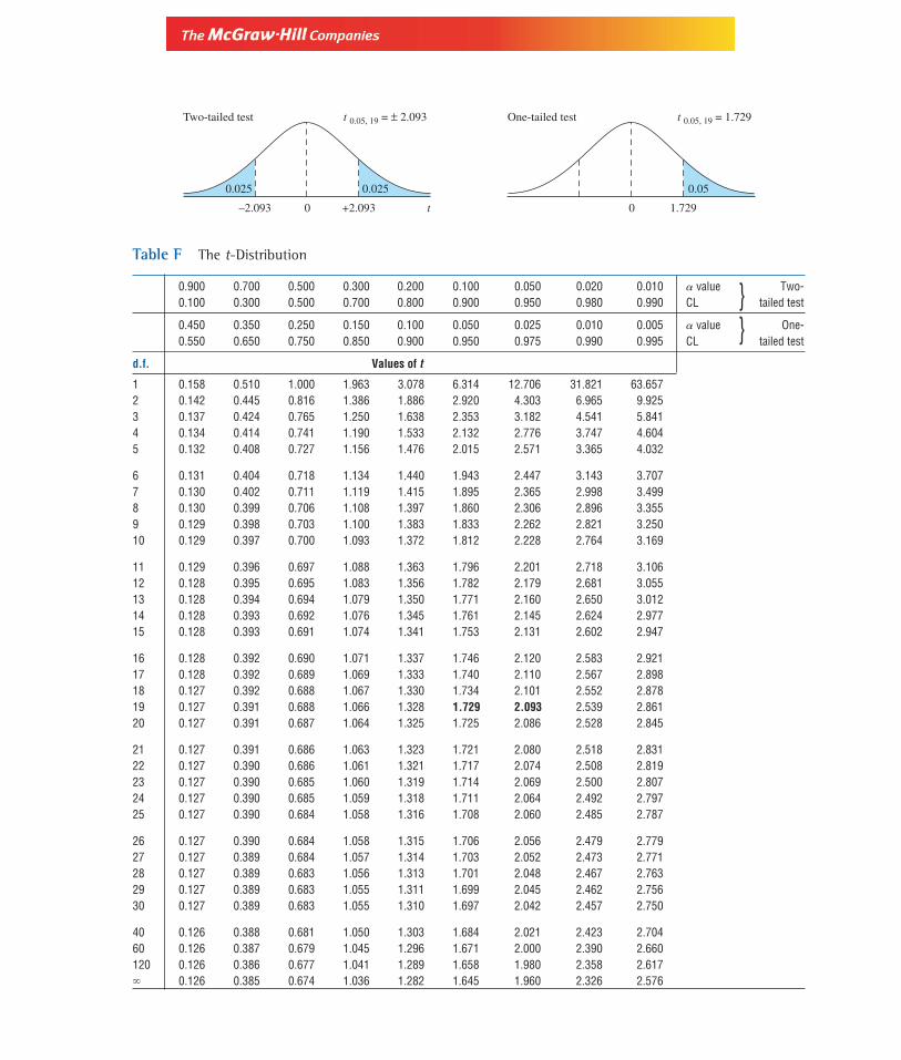
Version, Third Edition
Table F The t-Distribution
0.900 0.700 0.500 0.300 0.200 0.100 0.050 0.020 0.010 a value Two-0.100 0.300 0.500 0.700 0.800 0.900 0.950 0.980 0.990 CL tailed test
0.450 0.350 0.250 0.150 0.100 0.050 0.025 0.010 0.005 a value One-0.550 0.650 0.750 0.850 0.900 0.950 0.975 0.990 0.995 CL tailed test
d.f. Values of t
1 0.158 0.510 1.000 1.963 3.078 6.314 12.706 31.821 63.6572 0.142 0.445 0.816 1.386 1.886 2.920 4.303 6.965 9.9253 0.137 0.424 0.765 1.250 1.638 2.353 3.182 4.541 5.8414 0.134 0.414 0.741 1.190 1.533 2.132 2.776 3.747 4.6045 0.132 0.408 0.727 1.156 1.476 2.015 2.571 3.365 4.032
6 0.131 0.404 0.718 1.134 1.440 1.943 2.447 3.143 3.7077 0.130 0.402 0.711 1.119 1.415 1.895 2.365 2.998 3.4998 0.130 0.399 0.706 1.108 1.397 1.860 2.306 2.896 3.3559 0.129 0.398 0.703 1.100 1.383 1.833 2.262 2.821 3.25010 0.129 0.397 0.700 1.093 1.372 1.812 2.228 2.764 3.169
11 0.129 0.396 0.697 1.088 1.363 1.796 2.201 2.718 3.10612 0.128 0.395 0.695 1.083 1.356 1.782 2.179 2.681 3.05513 0.128 0.394 0.694 1.079 1.350 1.771 2.160 2.650 3.01214 0.128 0.393 0.692 1.076 1.345 1.761 2.145 2.624 2.97715 0.128 0.393 0.691 1.074 1.341 1.753 2.131 2.602 2.947
16 0.128 0.392 0.690 1.071 1.337 1.746 2.120 2.583 2.92117 0.128 0.392 0.689 1.069 1.333 1.740 2.110 2.567 2.89818 0.127 0.392 0.688 1.067 1.330 1.734 2.101 2.552 2.87819 0.127 0.391 0.688 1.066 1.328 1.729 2.093 2.539 2.86120 0.127 0.391 0.687 1.064 1.325 1.725 2.086 2.528 2.845
21 0.127 0.391 0.686 1.063 1.323 1.721 2.080 2.518 2.83122 0.127 0.390 0.686 1.061 1.321 1.717 2.074 2.508 2.81923 0.127 0.390 0.685 1.060 1.319 1.714 2.069 2.500 2.80724 0.127 0.390 0.685 1.059 1.318 1.711 2.064 2.492 2.79725 0.127 0.390 0.684 1.058 1.316 1.708 2.060 2.485 2.787
26 0.127 0.390 0.684 1.058 1.315 1.706 2.056 2.479 2.77927 0.127 0.389 0.684 1.057 1.314 1.703 2.052 2.473 2.77128 0.127 0.389 0.683 1.056 1.313 1.701 2.048 2.467 2.76329 0.127 0.389 0.683 1.055 1.311 1.699 2.045 2.462 2.75630 0.127 0.389 0.683 1.055 1.310 1.697 2.042 2.457 2.750
40 0.126 0.388 0.681 1.050 1.303 1.684 2.021 2.423 2.70460 0.126 0.387 0.679 1.045 1.296 1.671 2.000 2.390 2.660120 0.126 0.386 0.677 1.041 1.289 1.658 1.980 2.358 2.617� 0.126 0.385 0.674 1.036 1.282 1.645 1.960 2.326 2.576
Two-tailed test
0.025
0 t
0.025
–2.093 +2.093
t 0.05, 19 = ± 2.093 One-tailed test
0.05
0 1.729
t 0.05, 19 = 1.729
}}