Applied Mathematics 225

Unit 2: Advanced numerical linear algebra

Lecturer: Chris H. Rycroft

Prologue: linking to objects and libraries in C++

As C++ programs grow in length, it becomes less desirable tocompile a single monolithic .cc file each time.

We aim to structure our program around C++ classes,self-contained functions, etc. that we want to re-use withoutrecompiling each time. C++ provides us with a mechanism fordoing this.

When compiling a C++ program, the final stage is linking, wherethe compiler searches for precompiled code to link into the currentexecutable

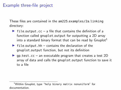
Example three-file project

These files are contained in the am225 examples/2a linkingdirectory:

I file output.cc – a file that contains the definition of afunction called gnuplot output for outputting a 2D arrayinto a standard binary format that can be read by Gnuplot1

I file output.hh – contains the declaration of thegnuplot output function, but not its definition

I gp test.cc – an executable program that creates a test 2Darray of data and calls the gnuplot output function to save itto a file

1Within Gnuplot, type “help binary matrix nonuniform” fordocumentation.

Structure of gp test.cc

#include <cmath>

#include "file_output.hh"

int main() {

// Code ...

gnuplot_output("test_out.gnu",fld,m,n,ax,bx,ay,by);

// Code ...}

The program includes file output.hh, so the compiler knowsabout the existence of the gnuplot output function.

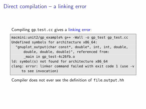
Direct compilation – a linking error

Compiling gp test.cc gives a linking error:

macmini:unit2/gp_example% g++ -Wall -o gp_test gp_test.ccUndefined symbols for architecture x86_64:"gnuplot_output(char const*, double*, int, int, double,

double, double, double)", referenced from:_main in gp_test-4c26fb.o

ld: symbol(s) not found for architecture x86_64clang: error: linker command failed with exit code 1 (use -v

to see invocation)

Compiler does not ever see the definition of file output.hh

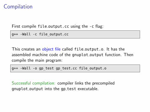
Compilation

First compile file output.cc using the -c flag:

g++ -Wall -c file_output.cc

This creates an object file called file output.o. It has theassembled machine code of the gnuplot output function. Thencompile the main program:

g++ -Wall -o gp_test gp_test.cc file_output.o

Successful compilation: compiler links the precompiledgnuplot output into the gp test executable.

Build system

A project could consist of multiple object files and multipleexecutables.

Object files need to be built prior to linking to executables. Someobject files might depend on others.

To simplify compilation we need a build system. We demonstratethe use of GNU Make2 although there are many others.

A file called “Makefile” contains the dependencies betweenprograms. Typing “make” on the command line recompiles onlythe files whose date stamps indicate they are out of date.

2https://www.gnu.org/software/make/

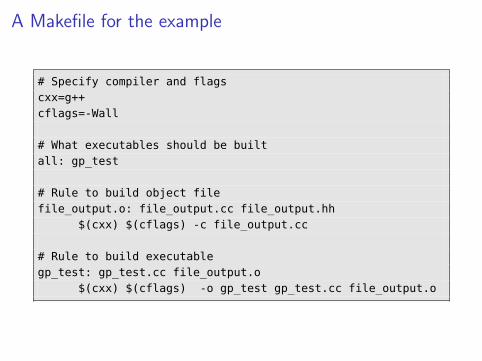
A Makefile for the example

# Specify compiler and flagscxx=g++cflags=-Wall

# What executables should be builtall: gp_test

# Rule to build object filefile_output.o: file_output.cc file_output.hh

$(cxx) $(cflags) -c file_output.cc

# Rule to build executablegp_test: gp_test.cc file_output.o

$(cxx) $(cflags) -o gp_test gp_test.cc file_output.o

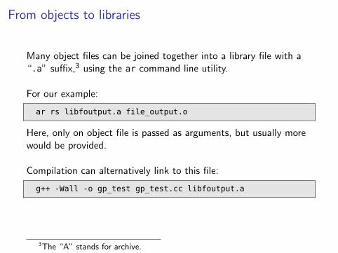
From objects to libraries

Many object files can be joined together into a library file with a“.a” suffix,3 using the ar command line utility.

For our example:

ar rs libfoutput.a file_output.o

Here, only on object file is passed as arguments, but usually morewould be provided.

Compilation can alternatively link to this file:

g++ -Wall -o gp_test gp_test.cc libfoutput.a

3The “A” stands for archive.

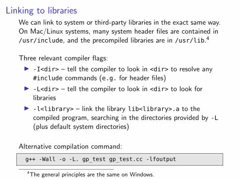
Linking to librariesWe can link to system or third-party libraries in the exact same way.On Mac/Linux systems, many system header files are contained in/usr/include, and the precompiled libraries are in /usr/lib.4

Three relevant compiler flags:

I -I<dir> – tell the compiler to look in <dir> to resolve any#include commands (e.g. for header files)

I -L<dir> – tell the compiler to look in <dir> to look forlibraries

I -l<library> – link the library lib<library>.a to thecompiled program, searching in the directories provided by -L(plus default system directories)

Alternative compilation command:

g++ -Wall -o -L. gp_test gp_test.cc -lfoutput

4The general principles are the same on Windows.

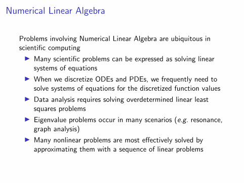
Numerical Linear Algebra

Problems involving Numerical Linear Algebra are ubiquitous inscientific computing

I Many scientific problems can be expressed as solving linearsystems of equations

I When we discretize ODEs and PDEs, we frequently need tosolve systems of equations for the discretized function values

I Data analysis requires solving overdetermined linear leastsquares problems

I Eigenvalue problems occur in many scenarios (e.g. resonance,graph analysis)

I Many nonlinear problems are most effectively solved byapproximating them with a sequence of linear problems

Topics covered in AM2055

I The LU factorization

I The QR decomposition

I Singular Value Decomposition

I Eigenvalue algorithms (power method, Rayleigh quotient,Krylov methods)

I Multigrid method

5See AM205 units 2 and 5.

Topics we will cover

We will examine the design of two widely-used and powerfullibraries, BLAS and LAPACK, for numerical linear algebra.

We will look at Krylov methods for the solution of linear algebraproblems, and the associated issue of preconditioning.

We will look at the Fast Fourier Transform, which can be viewedas a solution method for many matrix problems of interest.

We will look at domain decomposition for parallelizing numericallinear algebra routines.

Book

We will make use of the following textbook, and follow itsnotation:

I James W. Demmel, Applied Numerical Linear Algebra, SIAM,1997.

Numerical linear algebra is an active area of research, with muchinterest in efficient parallel methods for supercomputingapplications.

One issue is fault tolerance. When running on 105 CPUs,probability of failure on one of CPU is high. Aim for algorithmsthat can deal with this failure.

Some history

Since linear algebra often reduces to model problems (i.e. solveAx = b, find the eigenvalues of A) it is well-suited to being solvedby libraries.

An early library was LINPACK,6 used on supercomputers in the1970s and 1980s. The LINPACK benchmark is still used to test thespeed of supercomputers in the TOP5007 list.

LINPACK was designed before modern memory hierarchies becameimportant for optimal performance. Is has largely been supersededby BLAS (Basic Linear Algebra Subroutines) and LAPACK (LinearAlgebra PACKage), which take memory hierarchies into account.

6http://www.netlib.org/linpack/7https://www.top500.org

Example

Define tarith as the time to do a floating point operation and tmem

as the time to move memory between hierarchy levels. Assumetarith � tmem on modern systems.

Consider adding two n × n matrices together. We can’t do anybetter than the following procedure on each matrix entry:

I Read the two numbers from memory (2tmem)

I Add the two numbers (tarith)

I Store the result in memory (tmem)

Total time is n2(3tmem + tarith).

A measure of memory efficiency

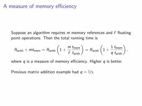
Suppose an algorithm requires m memory references and f floatingpoint operations. Then the total running time is

ftarith + mtmem = ftarith

(1 +

m

f

tmem

tarith

)= ftarith

(1 +

1

q

tmem

tarith

),

where q is a measure of memory efficiency. Higher q is better.

Previous matrix addition example had q = 1/3.

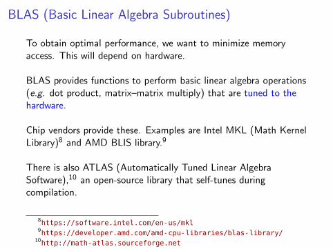
BLAS (Basic Linear Algebra Subroutines)

To obtain optimal performance, we want to minimize memoryaccess. This will depend on hardware.

BLAS provides functions to perform basic linear algebra operations(e.g. dot product, matrix–matrix multiply) that are tuned to thehardware.

Chip vendors provide these. Examples are Intel MKL (Math KernelLibrary)8 and AMD BLIS library.9

There is also ATLAS (Automatically Tuned Linear AlgebraSoftware),10 an open-source library that self-tunes duringcompilation.

8https://software.intel.com/en-us/mkl9https://developer.amd.com/amd-cpu-libraries/blas-library/

10http://math-atlas.sourceforge.net

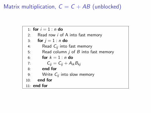
Matrix multiplication, C = C + AB (unblocked)

1: for i = 1 : n do2: Read row i of A into fast memory3: for j = 1 : n do4: Read Cij into fast memory5: Read column j of B into fast memory6: for k = 1 : n do7: Cij = Cij + AikBkj

8: end for9: Write Cij into slow memory

10: end for11: end for

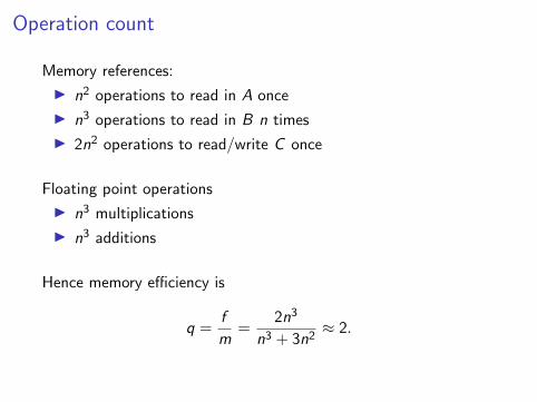
Operation count

Memory references:

I n2 operations to read in A once

I n3 operations to read in B n times

I 2n2 operations to read/write C once

Floating point operations

I n3 multiplications

I n3 additions

Hence memory efficiency is

q =f

m=

2n3

n3 + 3n2≈ 2.

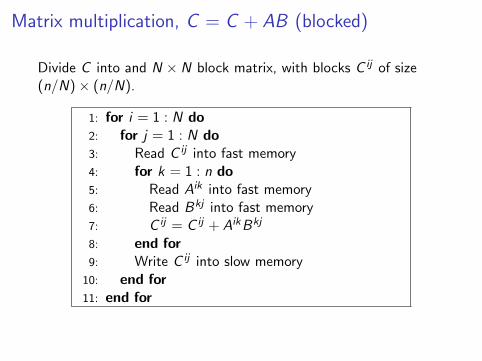
Matrix multiplication, C = C + AB (blocked)

Divide C into and N × N block matrix, with blocks C ij of size(n/N)× (n/N).

1: for i = 1 : N do2: for j = 1 : N do3: Read C ij into fast memory4: for k = 1 : n do5: Read Aik into fast memory6: Read Bkj into fast memory7: C ij = C ij + AikBkj

8: end for9: Write C ij into slow memory

10: end for11: end for

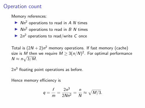
Operation count

Memory references:

I Nn2 operations to read in A N times

I Nn2 operations to read in B N times

I 2n2 operations to read/write C once

Total is (2N + 2)n2 memory operations. If fast memory (cache)size is M then we require M ≥ 3(n/N)2. For optimal performanceN ≈ n

√3/M.

2n3 floating point operations as before.

Hence memory efficiency is

q =f

m=

2n3

2Nn2=

n

N≈√

M/3.

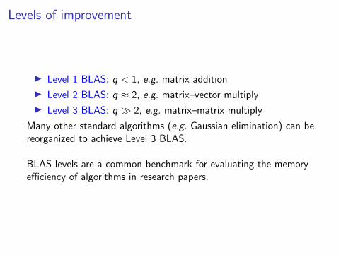
Levels of improvement

I Level 1 BLAS: q < 1, e.g. matrix addition

I Level 2 BLAS: q ≈ 2, e.g. matrix–vector multiply

I Level 3 BLAS: q � 2, e.g. matrix–matrix multiply

Many other standard algorithms (e.g. Gaussian elimination) can bereorganized to achieve Level 3 BLAS.

BLAS levels are a common benchmark for evaluating the memoryefficiency of algorithms in research papers.

BLAS matrix–matrix multiply example

Computer demo: timing comparison using BLAS routine.

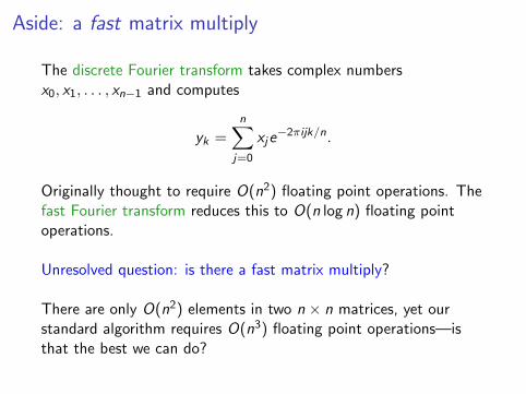
Aside: a fast matrix multiply

The discrete Fourier transform takes complex numbersx0, x1, . . . , xn−1 and computes

yk =n∑

j=0

xje−2πijk/n.

Originally thought to require O(n2) floating point operations. Thefast Fourier transform reduces this to O(n log n) floating pointoperations.

Unresolved question: is there a fast matrix multiply?

There are only O(n2) elements in two n × n matrices, yet ourstandard algorithm requires O(n3) floating point operations—isthat the best we can do?

Aside: a fast matrix multiply

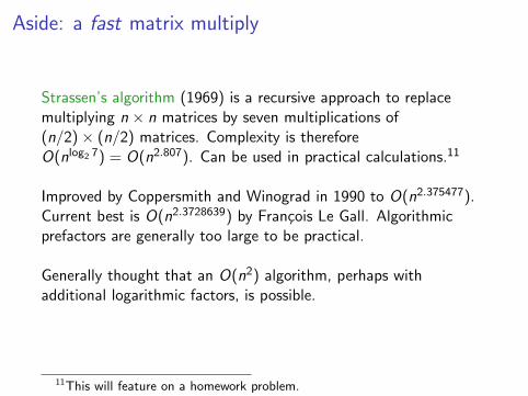
Strassen’s algorithm (1969) is a recursive approach to replacemultiplying n × n matrices by seven multiplications of(n/2)× (n/2) matrices. Complexity is thereforeO(nlog2 7) = O(n2.807). Can be used in practical calculations.11

Improved by Coppersmith and Winograd in 1990 to O(n2.375477).Current best is O(n2.3728639) by Francois Le Gall. Algorithmicprefactors are generally too large to be practical.

Generally thought that an O(n2) algorithm, perhaps withadditional logarithmic factors, is possible.

11This will feature on a homework problem.

LAPACK

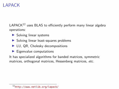
LAPACK12 uses BLAS to efficiently perform many linear algebraoperations:

I Solving linear systems

I Solving linear least-squares problems

I LU, QR, Cholesky decompositions

I Eigenvalue computations

It has specialized algorithms for banded matrices, symmetricmatrices, orthogonal matrices, Hessenberg matrices, etc.

12http://www.netlib.org/lapack/

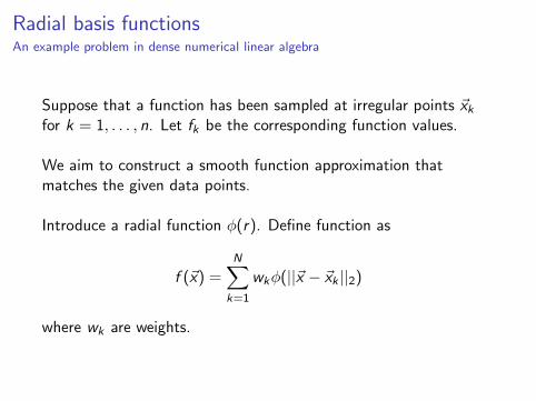
Radial basis functionsAn example problem in dense numerical linear algebra

Suppose that a function has been sampled at irregular points ~xkfor k = 1, . . . , n. Let fk be the corresponding function values.

We aim to construct a smooth function approximation thatmatches the given data points.

Introduce a radial function φ(r). Define function as

f (~x) =N∑

k=1

wkφ(||~x − ~xk ||2)

where wk are weights.

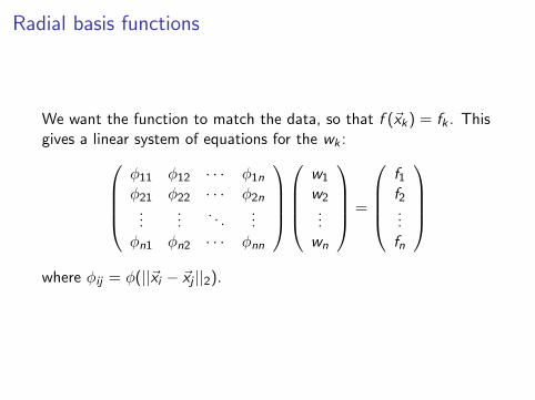
Radial basis functions

We want the function to match the data, so that f (~xk) = fk . Thisgives a linear system of equations for the wk :

φ11 φ12 · · · φ1nφ21 φ22 · · · φ2n

......

. . ....

φn1 φn2 · · · φnn

w1

w2...wn

=

f1f2...fn

where φij = φ(||~xi − ~xj ||2).

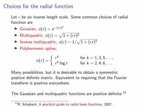
Choices for the radial function

Let ε be an inverse length scale. Some common choices of radialfunction are

I Gaussian, φ(r) = e−(εr)2

I Multiquadric, φ(r) =√

1 + (εr)2

I Inverse multiquadric, φ(r) = 1/√

1 + (εr)2

I Polyharmonic spline,

φ(r) =

{rk for k = 1, 3, 5, . . .,rk log r for k = 2, 4, 6, . . .

Many possibilities, but it is desirable to obtain a symmetricpositive definite matrix. Equivalent to requiring that the Fouriertransform is positive everywhere.

The Gaussian and multiquadric functions are positive definite.13

13R. Schaback, A practical guide to radial basis functions, 2007.

Using LAPACK to solve dense linear systems

Computer demo: using LAPACK to compute radial basis functioninterpolations

Krylov methods revisited14

Given a matrix A and vector b, a Krylov sequence is the set ofvectors

{b,Ab,A2b,A3b, . . .}

The corresponding Krylov subspaces are the spaces spanned bysuccessive groups of these vectors

Km(A, b) ≡ span{b,Ab,A2b, . . . ,Am−1b}

An important advantage: Krylov methods do not deal directly withA, but rather with matrix–vector products involving A

This is particularly helpful when A is large and sparse, sincematrix–vector multiplications are relatively cheap

14This is a quick review of material from AM205 unit 5.

Arnoldi Iteration

We define a matrix as being in Hessenberg form in the followingway:

I A is called upper-Hessenberg if aij = 0 for all i > j + 1

I A is called lower-Hessenberg if aij = 0 for all j > i + 1

The Arnoldi iteration is a Krylov subspace iterative method thatreduces A to upper-Hessenberg form

Arnoldi Iteration

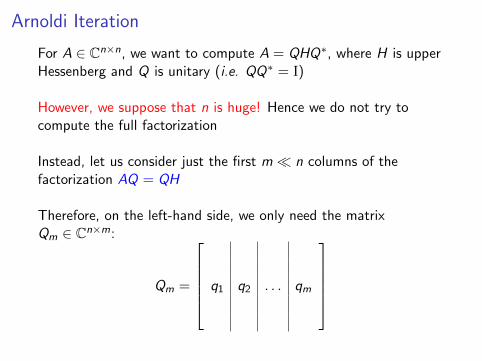
For A ∈ Cn×n, we want to compute A = QHQ∗, where H is upperHessenberg and Q is unitary (i.e. QQ∗ = I)

However, we suppose that n is huge! Hence we do not try tocompute the full factorization

Instead, let us consider just the first m� n columns of thefactorization AQ = QH

Therefore, on the left-hand side, we only need the matrixQm ∈ Cn×m:

Qm =

q1 q2 . . . qm

Arnoldi Iteration

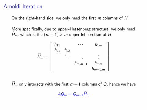
On the right-hand side, we only need the first m columns of H

More specifically, due to upper-Hessenberg structure, we only needHm, which is the (m + 1)×m upper-left section of H:

Hm =

h11 · · · h1mh21 h22

. . .. . .

...hm,m−1 hmm

hm+1,m

Hm only interacts with the first m+ 1 columns of Q, hence we have

AQm = Qm+1Hm

Arnoldi Iteration

A

q1 . . . qm

=

q1 . . . qm+1

h11 · · · h1mh21 · · · h2m

. . ....

hm+1,m

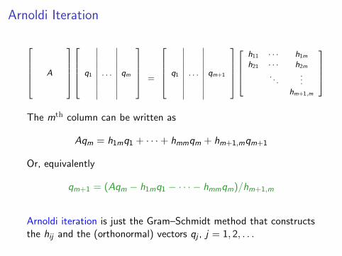
The mth column can be written as

Aqm = h1mq1 + · · ·+ hmmqm + hm+1,mqm+1

Or, equivalently

qm+1 = (Aqm − h1mq1 − · · · − hmmqm)/hm+1,m

Arnoldi iteration is just the Gram–Schmidt method that constructsthe hij and the (orthonormal) vectors qj , j = 1, 2, . . .

Arnoldi Iteration

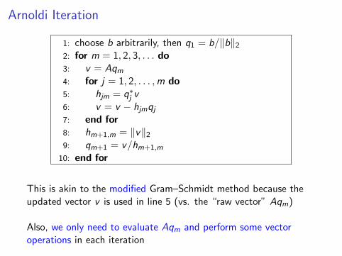
1: choose b arbitrarily, then q1 = b/‖b‖22: for m = 1, 2, 3, . . . do3: v = Aqm4: for j = 1, 2, . . . ,m do5: hjm = q∗j v6: v = v − hjmqj7: end for8: hm+1,m = ‖v‖29: qm+1 = v/hm+1,m

10: end for

This is akin to the modified Gram–Schmidt method because theupdated vector v is used in line 5 (vs. the “raw vector” Aqm)

Also, we only need to evaluate Aqm and perform some vectoroperations in each iteration

Lanczos Iteration

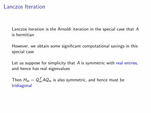
Lanczos iteration is the Arnoldi iteration in the special case that Ais hermitian

However, we obtain some significant computational savings in thisspecial case

Let us suppose for simplicity that A is symmetric with real entries,and hence has real eigenvalues

Then Hm = QTmAQm is also symmetric, and hence must be

tridiagonal

Lanczos Iteration

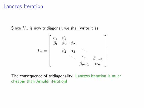
Since Hm is now tridiagonal, we shall write it as

Tm =

α1 β1β1 α2 β2

β2 α3. . .

. . .. . . βm−1βm−1 αm

The consequence of tridiagonality: Lanczos iteration is muchcheaper than Arnoldi iteration!

Lanczos Iteration

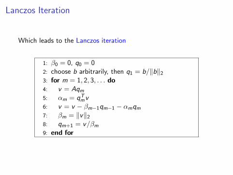
Which leads to the Lanczos iteration

1: β0 = 0, q0 = 02: choose b arbitrarily, then q1 = b/‖b‖23: for m = 1, 2, 3, . . . do4: v = Aqm5: αm = qTmv6: v = v − βm−1qm−1 − αmqm7: βm = ‖v‖28: qm+1 = v/βm9: end for

Solving linear systems with Krylov methods

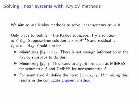
We aim to use Krylov methods to solve linear systems Ax = b

Only place to look is in the Krylov subspace. Try a solutionxk ∈ Kk . Suppose true solution is x = A−1b and residual isrk = b − Axk . Could aim for

I Minimizing ‖xk − x‖2. There is not enough information in theKrylov subspace to do this.

I Minimizing ‖rk‖2. This leads to algorithms such as MINRESfor symmetric A and GMRES for nonsymmetric A.

I For symmetric A, define the norm ‖x − xk‖A. Minimizing thisresults in the conjugate gradient method.

Conjugate Gradient Method

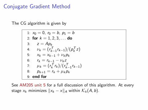
The CG algorithm is given by

1: x0 = 0, r0 = b, p1 = b2: for k = 1, 2, 3, . . . do3: z = Apk4: νk = (rTk−1rk−1)/(pTk z)5: xk = xk−1 + νkpk6: rk = rk−1 − νkz7: µk = (rTk rk)/(rTk−1rk−1)8: pk+1 = rk + µkpk9: end for

See AM205 unit 5 for a full discussion of this algorithm. At everystage xk minimizes ‖xk − x‖A within Kk(A, b).

Basic conjugate gradient example

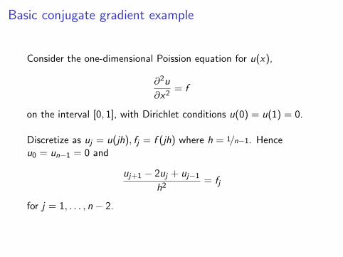
Consider the one-dimensional Poission equation for u(x),

∂2u

∂x2= f

on the interval [0, 1], with Dirichlet conditions u(0) = u(1) = 0.

Discretize as uj = u(jh), fj = f (jh) where h = 1/n−1. Henceu0 = un−1 = 0 and

uj+1 − 2uj + uj−1h2

= fj

for j = 1, . . . , n − 2.

Basic conjugate gradient example

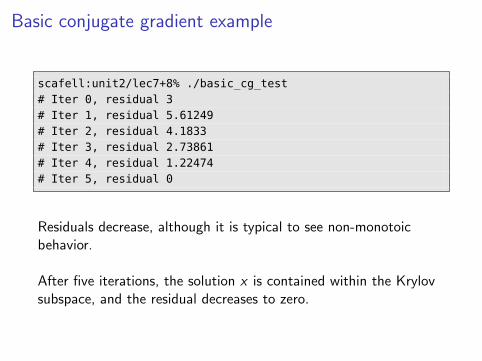
scafell:unit2/lec7+8% ./basic_cg_test# Iter 0, residual 3# Iter 1, residual 5.61249# Iter 2, residual 4.1833# Iter 3, residual 2.73861# Iter 4, residual 1.22474# Iter 5, residual 0

Residuals decrease, although it is typical to see non-monotoicbehavior.

After five iterations, the solution x is contained within the Krylovsubspace, and the residual decreases to zero.

Compactly supported radial basis functions

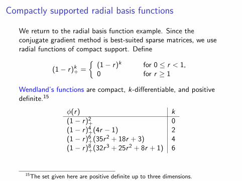
We return to the radial basis function example. Since theconjugate gradient method is best-suited sparse matrices, we useradial functions of compact support. Define

(1− r)k+ =

{(1− r)k for 0 ≤ r < 1,0 for r ≥ 1

Wendland’s functions are compact, k-differentiable, and positivedefinite.15

φ(r) k

(1− r)2+ 0(1− r)4+(4r − 1) 2(1− r)6+(35r2 + 18r + 3) 4(1− r)8+(32r3 + 25r2 + 8r + 1) 6

15The set given here are positive definite up to three dimensions.

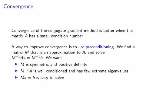
Convergence

Convergence of the conjugate gradient method is better when thematrix A has a small condition number

A way to improve convergence is to use preconditioning. We find amatrix M that is an approximation to A, and solveM−1Ax = M−1b. We want

I M is symmetric and positive definite

I M−1A is well conditioned and has few extreme eigenvalues

I Mx = b is easy to solve

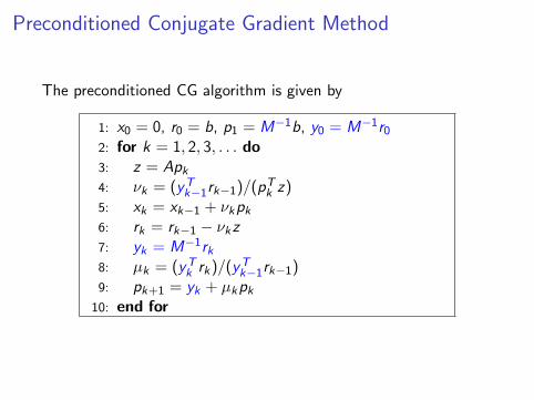
Preconditioned Conjugate Gradient Method

The preconditioned CG algorithm is given by

1: x0 = 0, r0 = b, p1 = M−1b, y0 = M−1r02: for k = 1, 2, 3, . . . do3: z = Apk4: νk = (yTk−1rk−1)/(pTk z)5: xk = xk−1 + νkpk6: rk = rk−1 − νkz7: yk = M−1rk8: µk = (yTk rk)/(yTk−1rk−1)9: pk+1 = yk + µkpk

10: end for

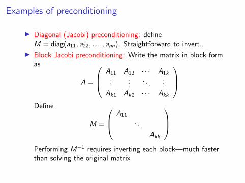
Examples of preconditioning

I Diagonal (Jacobi) preconditioning: defineM = diag(a11, a22, . . . , ann). Straightforward to invert.

I Block Jacobi preconditioning: Write the matrix in block formas

A =

A11 A12 · · · A1k...

.... . .

...Ak1 Ak2 · · · Akk

Define

M =

A11

. . .

Akk

Performing M−1 requires inverting each block—much fasterthan solving the original matrix

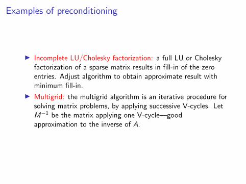
Examples of preconditioning

I Incomplete LU/Cholesky factorization: a full LU or Choleskyfactorization of a sparse matrix results in fill-in of the zeroentries. Adjust algorithm to obtain approximate result withminimum fill-in.

I Multigrid: the multigrid algorithm is an iterative procedure forsolving matrix problems, by applying successive V-cycles. LetM−1 be the matrix applying one V-cycle—goodapproximation to the inverse of A.

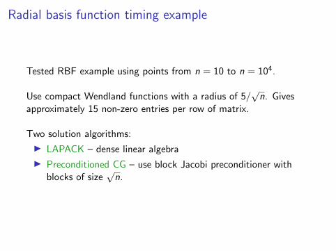
Radial basis function timing example

Tested RBF example using points from n = 10 to n = 104.

Use compact Wendland functions with a radius of 5/√n. Gives

approximately 15 non-zero entries per row of matrix.

Two solution algorithms:

I LAPACK – dense linear algebra

I Preconditioned CG – use block Jacobi preconditioner withblocks of size

√n.

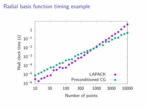
Radial basis function timing example

10−6

10−5

10−4

10−3

10−2

10−1

1

10 30 100 300 1000 3000 10000

Wal

lcl

ock

tim

e(s

)

Number of points

LAPACKPreconditioned CG

Radial basis function timing example

For small systems with n < 800, dense linear algebra is faster.

For large systems with n ≥ 800, the O(n3) scaling of LAPACKmakes it inefficient.

Preconditioned CG has O(n2.37) scaling in this example, andtherefore becomes the best choice for large numbers of points.

This timing comparison is heavily dependent on the matrixstructure and sparsity. LAPACK does better for denser matrices.

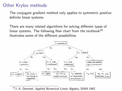
Other Krylov methods

The conjugate gradient method only applies to symmetric positivedefinite linear systems.

There are many related algorithms for solving different types oflinear systems. The following flow chart from the textbook16

illustrates some of the different possibilities.

16J. A. Demmel, Applied Numerical Linear Algebra, SIAM 1997.

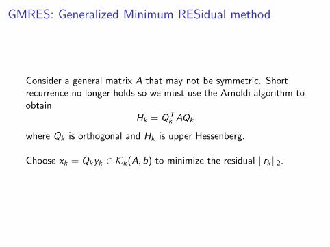
GMRES: Generalized Minimum RESidual method

Consider a general matrix A that may not be symmetric. Shortrecurrence no longer holds so we must use the Arnoldi algorithm toobtain

Hk = QTk AQk

where Qk is orthogonal and Hk is upper Hessenberg.

Choose xk = Qkyk ∈ Kk(A, b) to minimize the residual ‖rk‖2.

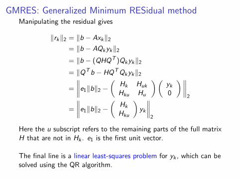
GMRES: Generalized Minimum RESidual methodManipulating the residual gives

‖rk‖2 = ‖b − Axk‖2= ‖b − AQkyk‖2= ‖b − (QHQT )Qkyk‖2= ‖QTb − HQTQkyk‖2

=

∥∥∥∥e1‖b‖2 − ( Hk Huk

Hku Hu

)(yk0

)∥∥∥∥2

=

∥∥∥∥e1‖b‖2 − ( Hk

Hku

)yk

∥∥∥∥2

Here the u subscript refers to the remaining parts of the full matrixH that are not in Hk . e1 is the first unit vector.

The final line is a linear least-squares problem for yk , which can besolved using the QR algorithm.

GMRES: solving the least-squares problem

Normally, performing a QR factorization would require O(k3)iterations.

But here, we require the QR factorization of the (k + 1)× kHessenberg matrix. We can perform the QR factorization byperforming k Givens rotations to rotate out the terms below thediagonal.

GMRES requires O(kn) memory to store the vectors Qk . A variantto minimize the growth of computation and storage is to stop afterk steps, and restart by solving Ad = rk = b − Axk , after which thesolution is given by d + xk .

This is called GMRES(k). It is still more expensive than conjugategradient.

The Fast Fourier Transform

Consider a one-dimensional Poisson problem

−d2v

dx2= f (x)

for a function v(x) on [0, 1] with boundary conditionsv(0) = v(1) = 0.

Discretize with N + 2 evenly spaced points with grid spacingh = 1/(N + 1), so that xi = hi .

Second-order centered finite difference gives

−vi−1 + 2vi − vi+1 = h2fi

for i = 1, . . .N.

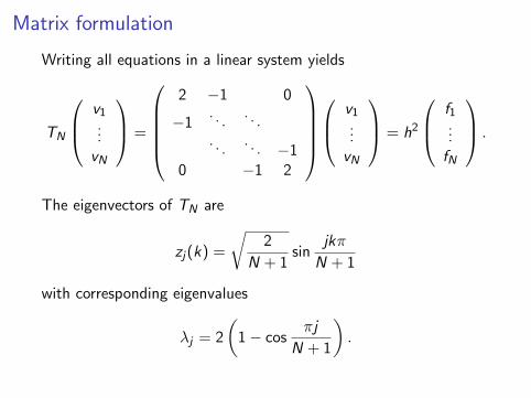
Matrix formulation

Writing all equations in a linear system yields

TN

v1...vN

=

2 −1 0

−1. . .

. . .. . .

. . . −10 −1 2

v1

...vN

= h2

f1...fN

.

The eigenvectors of TN are

zj(k) =

√2

N + 1sin

jkπ

N + 1

with corresponding eigenvalues

λj = 2

(1− cos

πj

N + 1

).

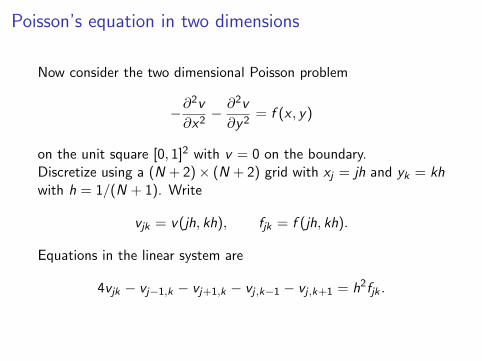
Poisson’s equation in two dimensions

Now consider the two dimensional Poisson problem

−∂2v

∂x2− ∂2v

∂y2= f (x , y)

on the unit square [0, 1]2 with v = 0 on the boundary.Discretize using a (N + 2)× (N + 2) grid with xj = jh and yk = khwith h = 1/(N + 1). Write

vjk = v(jh, kh), fjk = f (jh, kh).

Equations in the linear system are

4vjk − vj−1,k − vj+1,k − vj ,k−1 − vj ,k+1 = h2fjk .

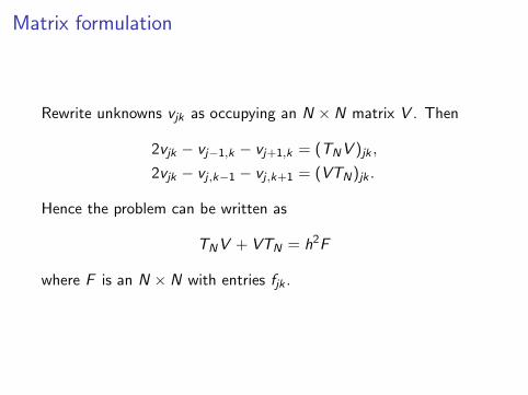
Matrix formulation

Rewrite unknowns vjk as occupying an N × N matrix V . Then

2vjk − vj−1,k − vj+1,k = (TNV )jk ,

2vjk − vj ,k−1 − vj ,k+1 = (VTN)jk .

Hence the problem can be written as

TNV + VTN = h2F

where F is an N × N with entries fjk .

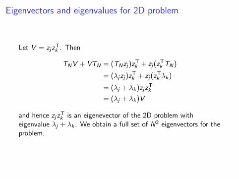
Eigenvectors and eigenvalues for 2D problem

Let V = zjzTk . Then

TNV + VTN = (TNzj)zTk + zj(z

Tk TN)

= (λjzj)zTk + zj(z

Tk λk)

= (λj + λk)zjzTk

= (λj + λk)V

and hence zjzTk is an eigenevector of the 2D problem with

eigenvalue λj + λk . We obtain a full set of N2 eigenvectors for theproblem.

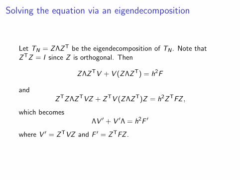
Solving the equation via an eigendecomposition

Let TN = ZΛZT be the eigendecomposition of TN . Note thatZTZ = I since Z is orthogonal. Then

ZΛZTV + V (ZΛZT) = h2F

andZTZΛZTVZ + ZTV (ZΛZT)Z = h2ZTFZ ,

which becomesΛV ′ + V ′Λ = h2F ′

where V ′ = ZTVZ and F ′ = ZTFZ .

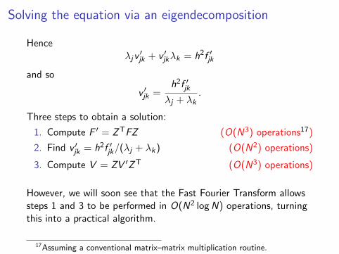
Solving the equation via an eigendecomposition

Henceλjv′jk + v ′jkλk = h2f ′jk

and so

v ′jk =h2f ′jkλj + λk

.

Three steps to obtain a solution:

1. Compute F ′ = ZTFZ (O(N3) operations17)

2. Find v ′jk = h2f ′jk/(λj + λk) (O(N2) operations)

3. Compute V = ZV ′ZT (O(N3) operations)

However, we will soon see that the Fast Fourier Transform allowssteps 1 and 3 to be performed in O(N2 logN) operations, turningthis into a practical algorithm.

17Assuming a conventional matrix–matrix multiplication routine.

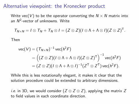
Alternative viewpoint: the Kronecker product

Write vec(V ) to be the operator converting the N × N matrix intoan N2-vector of unknowns. Write

TN×N = I ⊗ TN + TN ⊗ I = (Z ⊗ Z )(I ⊗ Λ + Λ⊗ I )(Z ⊗ Z )T.

Then

vec(V ) = (TN×N)−1 vec(h2F )

=(

(Z ⊗ Z )(I ⊗ Λ + Λ⊗ I )(Z ⊗ Z )T)−1

vec(h2F )

= (Z ⊗ Z )(I ⊗ Λ + Λ⊗ I )−1(ZT ⊗ ZT) vec(h2F ).

While this is less notationally elegant, it makes it clear that thesolution procedure could be extended to arbitrary dimensions.

i.e. in 3D, we would consider (Z ⊗ Z ⊗ Z ), applying the matrix Zto field values in each coordinate direction.

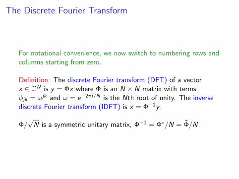
The Discrete Fourier Transform

For notational convenience, we now switch to numbering rows andcolumns starting from zero.

Definition: The discrete Fourier transform (DFT) of a vectorx ∈ CN is y = Φx where Φ is an N × N matrix with termsφjk = ωjk and ω = e−2πi/N is the Nth root of unity. The inversediscrete Fourier transform (IDFT) is x = Φ−1y .

Φ/√N is a symmetric unitary matrix, Φ−1 = Φ∗/N = Φ/N.

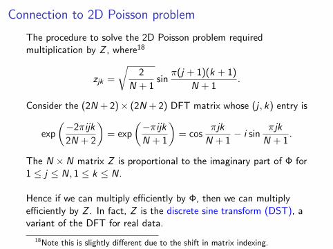
Connection to 2D Poisson problem

The procedure to solve the 2D Poisson problem requiredmultiplication by Z , where18

zjk =

√2

N + 1sin

π(j + 1)(k + 1)

N + 1.

Consider the (2N + 2)× (2N + 2) DFT matrix whose (j , k) entry is

exp

(−2πijk

2N + 2

)= exp

(−πijkN + 1

)= cos

πjk

N + 1− i sin

πjk

N + 1.

The N × N matrix Z is proportional to the imaginary part of Φ for1 ≤ j ≤ N, 1 ≤ k ≤ N.

Hence if we can multiply efficiently by Φ, then we can multiplyefficiently by Z . In fact, Z is the discrete sine transform (DST), avariant of the DFT for real data.

18Note this is slightly different due to the shift in matrix indexing.

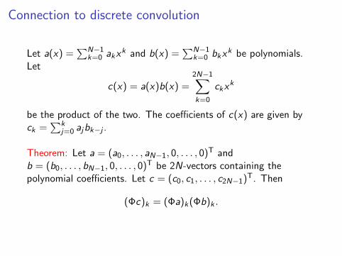
Connection to discrete convolution

Let a(x) =∑N−1

k=0 akxk and b(x) =

∑N−1k=0 bkx

k be polynomials.Let

c(x) = a(x)b(x) =2N−1∑k=0

ckxk

be the product of the two. The coefficients of c(x) are given byck =

∑kj=0 ajbk−j .

Theorem: Let a = (a0, . . . , aN−1, 0, . . . , 0)T andb = (b0, . . . , bN−1, 0, . . . , 0)T be 2N-vectors containing thepolynomial coefficients. Let c = (c0, c1, . . . , c2N−1)T. Then

(Φc)k = (Φa)k(Φb)k .

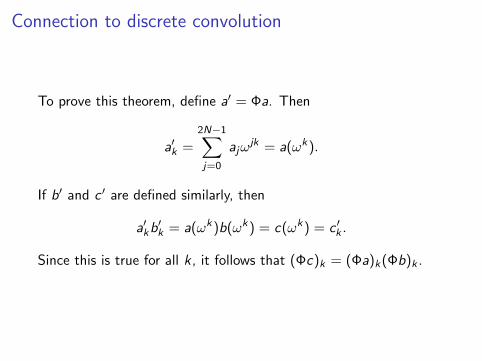
Connection to discrete convolution

To prove this theorem, define a′ = Φa. Then

a′k =2N−1∑j=0

ajωjk = a(ωk).

If b′ and c ′ are defined similarly, then

a′kb′k = a(ωk)b(ωk) = c(ωk) = c ′k .

Since this is true for all k , it follows that (Φc)k = (Φa)k(Φb)k .

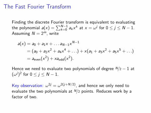
The Fast Fourier Transform

Finding the discrete Fourier transform is equivalent to evaluatingthe polynomial a(x) =

∑N−1k=0 akx

k at x = ωj for 0 ≤ j ≤ N − 1.Assuming N = 2m, write

a(x) = a0 + a1x + . . . aN−1xN−1

= (a0 + a2x2 + a4x

4 + . . .) + x(a1 + a3x2 + a5x

5 + . . .)

= aeven(x2) + xaodd(x2).

Hence we need to evaluate two polynomials of degree N/2− 1 at(ωj)2 for 0 ≤ j ≤ N − 1.

Key observation: ω2j = ω2(j+N/2), and hence we only need toevaluate the two polynomials at N/2 points. Reduces work by afactor of two.

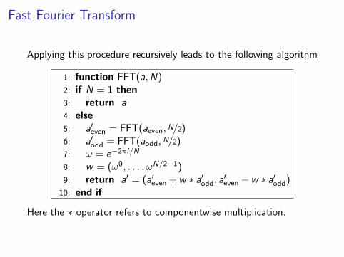
Fast Fourier Transform

Applying this procedure recursively leads to the following algorithm

1: function FFT(a,N)2: if N = 1 then3: return a4: else5: a′even = FFT(aeven, N/2)6: a′odd = FFT(aodd, N/2)7: ω = e−2πi/N

8: w = (ω0, . . . , ωN/2−1)9: return a′ = (a′even +w ∗ a′odd, a′even−w ∗ a′odd)

10: end if

Here the ∗ operator refers to componentwise multiplication.

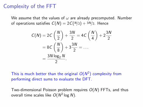
Complexity of the FFT

We assume that the values of ω are already precomputed. Numberof operations satisfies C (N) = 2C (N/2) + 3N/2. Hence

C (N) = 2C

(N

2

)+

3N

2= 4C

(N

4

)+ 2

3N

2

= 8C

(N

8

)+ 3

3N

2= . . .

=3N log2N

2.

This is much better than the original O(N2) complexity fromperforming direct sums to evaluate the DFT.

Two-dimensional Poisson problem requires O(N) FFTs, and thusoverall time scales like O(N2 logN).

Fast Fourier transform libraries

Chip vendors such as Intel provide tuned libraries for the FFT. TheIntel MKL contains FFT routines.

FFTW19 (www.fftw.org) is a widely-used open source library.

FFTW follows some similar design principles to BLAS, organizingcomputation in a cache-friendly manner, and exploiting vectorizedinstructions where possible.

FFTW provides very good performance across a wide range ofplatforms. While best perfomance is achieved for grid sizes N thatare powers of two, FFTW achieves O(N logN) performance forany grid size. Multithreaded and parallel routines available.

19Stands for “The Fastest Fourier Transform in the West”. Developed byMatteo Frigo and Steven Johnson at MIT.

Frequency analysis of music samples

Consider the following four music samples of length 0.1 s:

I Vocal sample from You Couldn’t Be Cuter by Sylvia McNair.This is a jazz standard, but McNair is primarily an operasinger.

I Vocal sample from Marry Me by St. Vincent.

I Vocal sample from It’s Alright, Ma (I’m Only Bleeding) byBob Dylan.

I Drum sample from Guess They Never Told You by TheAmerican Symphony of Soul. (Drums played by AM225 TFDan Fortunato.)

Samples were prepared using Audacity, which exports the soundsignal as single-precision floats. Contains stereo information (leftand right channels).

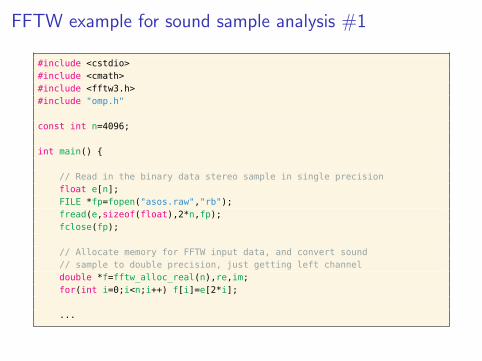
FFTW example for sound sample analysis #1

#include <cstdio>#include <cmath>#include <fftw3.h>#include "omp.h"

const int n=4096;

int main() {

// Read in the binary data stereo sample in single precisionfloat e[n];FILE *fp=fopen("asos.raw","rb");fread(e,sizeof(float),2*n,fp);fclose(fp);

// Allocate memory for FFTW input data, and convert sound// sample to double precision, just getting left channeldouble *f=fftw_alloc_real(n),re,im;for(int i=0;i<n;i++) f[i]=e[2*i];

...

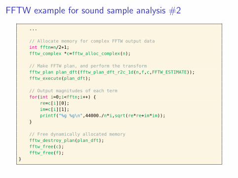
FFTW example for sound sample analysis #2

...

// Allocate memory for complex FFTW output dataint fftn=n/2+1;fftw_complex *c=fftw_alloc_complex(n);

// Make FFTW plan, and perform the transformfftw_plan plan_dft(fftw_plan_dft_r2c_1d(n,f,c,FFTW_ESTIMATE));fftw_execute(plan_dft);

// Output magnitudes of each termfor(int i=0;i<fftn;i++) {

re=c[i][0];im=c[i][1];printf("%g %g\n",44000./n*i,sqrt(re*re+im*im));

}

// Free dynamically allocated memoryfftw_destroy_plan(plan_dft);fftw_free(c);fftw_free(f);

}

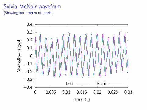
Sylvia McNair waveform(Showing both stereo channels)

−0.4

−0.3

−0.2

−0.1

0

0.1

0.2

0.3

0.4

0 0.005 0.01 0.015 0.02 0.025 0.03

Nor

mal

ized

sign

al

Time (s)

Left Right

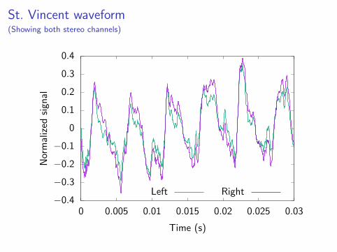
St. Vincent waveform(Showing both stereo channels)

−0.4

−0.3

−0.2

−0.1

0

0.1

0.2

0.3

0.4

0 0.005 0.01 0.015 0.02 0.025 0.03

Nor

mal

ized

sign

al

Time (s)

Left Right

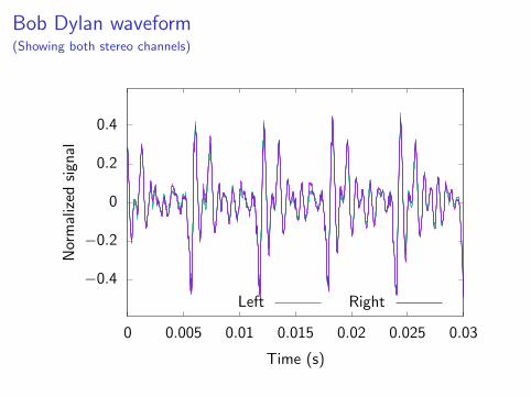
Bob Dylan waveform(Showing both stereo channels)

−0.4

−0.2

0

0.2

0.4

0 0.005 0.01 0.015 0.02 0.025 0.03

Nor

mal

ized

sign

al

Time (s)

Left Right

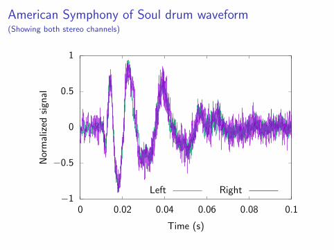
American Symphony of Soul drum waveform(Showing both stereo channels)

−1

−0.5

0

0.5

1

0 0.02 0.04 0.06 0.08 0.1

Nor

mal

ized

sign

al

Time (s)

Left Right

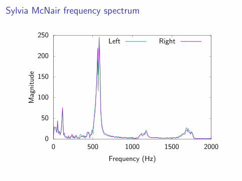
Sylvia McNair frequency spectrum

0

50

100

150

200

250

0 500 1000 1500 2000

Mag

nit

ud

e

Frequency (Hz)

Left Right

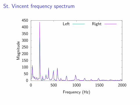
St. Vincent frequency spectrum

0

50

100

150

200

250

300

350

400

450

0 500 1000 1500 2000

Mag

nit

ud

e

Frequency (Hz)

Left Right

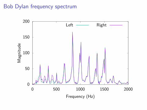
Bob Dylan frequency spectrum

0

50

100

150

200

0 500 1000 1500 2000

Mag

nit

ud

e

Frequency (Hz)

Left Right

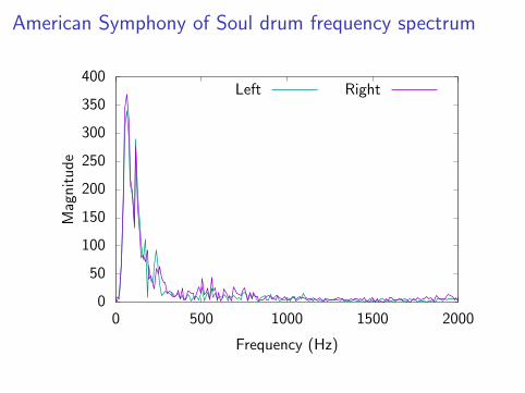
American Symphony of Soul drum frequency spectrum

0

50

100

150

200

250

300

350

400

0 500 1000 1500 2000

Mag

nit

ud

e

Frequency (Hz)

Left Right

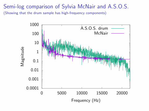
Semi-log comparison of Sylvia McNair and A.S.O.S.(Showing that the drum sample has high-frequency components)

0.0001

0.001

0.01

0.1

1

10

100

1000

0 5000 10000 15000 20000

Mag

nit

ud

e

Frequency (Hz)

A.S.O.S. drumMcNair

FFTW performance tuning and execution

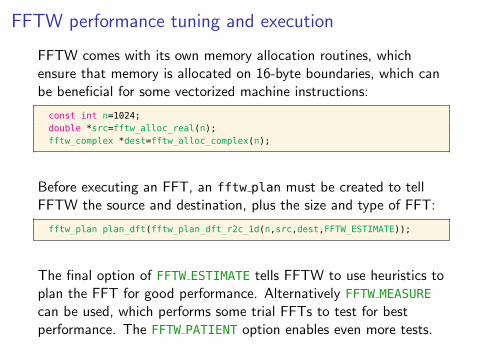
FFTW comes with its own memory allocation routines, whichensure that memory is allocated on 16-byte boundaries, which canbe beneficial for some vectorized machine instructions:

const int n=1024;double *src=fftw_alloc_real(n);fftw_complex *dest=fftw_alloc_complex(n);

Before executing an FFT, an fftw plan must be created to tellFFTW the source and destination, plus the size and type of FFT:

fftw_plan plan_dft(fftw_plan_dft_r2c_1d(n,src,dest,FFTW_ESTIMATE));

The final option of FFTW ESTIMATE tells FFTW to use heuristics toplan the FFT for good performance. Alternatively FFTW MEASUREcan be used, which performs some trial FFTs to test for bestperformance. The FFTW PATIENT option enables even more tests.

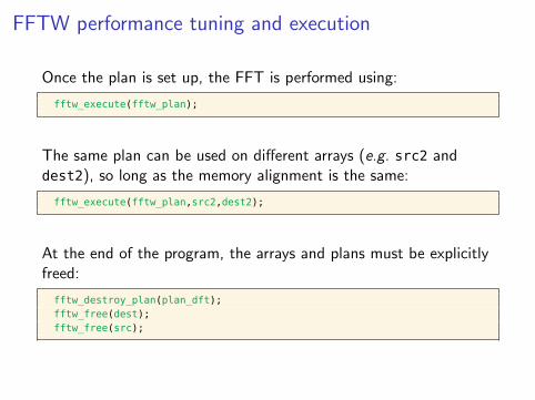
FFTW performance tuning and execution

Once the plan is set up, the FFT is performed using:

fftw_execute(fftw_plan);

The same plan can be used on different arrays (e.g. src2 anddest2), so long as the memory alignment is the same:

fftw_execute(fftw_plan,src2,dest2);

At the end of the program, the arrays and plans must be explicitlyfreed:

fftw_destroy_plan(plan_dft);fftw_free(dest);fftw_free(src);

Return to the 2D Poisson problem

In the last lecture we introduced a model 2D Poisson problem

−∂2v

∂x2− ∂2v

∂y2= f (x , y)

on the unit square [0, 1]2 with v = 0 on the boundary. Discretizedusing a (N + 2)× (N + 2) grid with xj = jh and yk = kh withh = 1/(N + 1).

Problem was rewritten as

TNV + VTN = h2F

where TN is a triangular matrix, V is a matrix containing thesolution, and F is a matrix containing the source term.

FFT solution method

Let TN = ZΛZT be the eigendecomposition of TN . Then asolution method is

1. Compute F ′ = ZTFZ

2. Find v ′jk = h2f ′jk/(λj + λk)

3. Compute V = ZV ′ZT

Multiplication be Z is equivalent to the one-dimensional discretesine transform, and thus can be solved efficiently with FFTW.

Computer demo: solution to the 2D Poisson equation using FFTW.

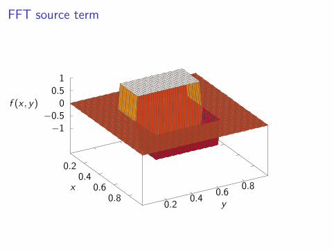
FFT source term

0.20.4

0.60.8

0.20.4

0.60.8

−1−0.5

00.5

1

x

y

f (x , y)

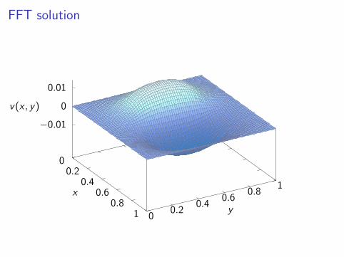
FFT solution

00.2

0.40.6

0.81 0

0.20.4

0.60.8

1

−0.01

0

0.01

x

y

v(x , y)

Testing convergence

The solution method to Poisson problem is based on asecond-order finite-difference stencil. We would like to test theactual convergence properties of the solution.

For a general equation and source term, it is difficult to write downan analytical solution.

An approach for cases like this is to use the method ofmanufactured solutions, by writing down the solution v , andfinding the source term that will give it.

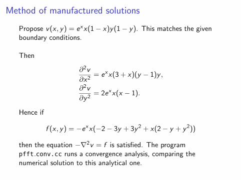
Method of manufactured solutions

Propose v(x , y) = exx(1− x)y(1− y). This matches the givenboundary conditions.

Then

∂2v

∂x2= exx(3 + x)(y − 1)y ,

∂2v

∂y2= 2exx(x − 1).

Hence if

f (x , y) = −exx(−2− 3y + 3y2 + x(2− y + y2))

then the equation −∇2v = f is satisfied. The programpfft conv.cc runs a convergence analysis, comparing thenumerical solution to this analytical one.

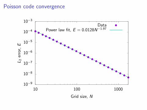
Poisson code convergence

10−9

10−8

10−7

10−6

10−5

10−4

10−3

10 100 1000

L2

erro

r,E

Grid size, N

DataPower law fit, E = 0.0128N−1.97

Comments on convergence

O(h2) convergence is achieved—this is expected since the solutionis based on a second-order stencil.

While the choice of f (x , y) is arbitrary, it is helpful to choosesomething that does not align with simple functions, or knowneigenfunctions of the system, to provide a better indication of thetypical behavior.

If the solution aligned with an eigenfunction, then the convergenceproperties may be atypical.

Spectral methods

The fast Fourier transform is also useful in the context of spectralmethods, a class of numerical methods for very accurately solvingproblems that feature smooth solutions.

We will not discuss spectral methods in detail, but we will give afew examples.

We aim to approximate a solution u(x) on some domain by a finitesum v(x) =

∑Nk=0 akφk(x) for some set of functions φk .

Spectral methods

A spectral method is characterized20 by the following threecharacteristics:

1. The approximations∑N

k=0 akφk(x) should converge rapidlyfor smooth functions.

2. Given coefficients ak it should be easy to determine bk suchthat

d

dx

(N∑

k=0

akφk(x)

)=

N∑k=0

bkφk(x)

3. It should be fast to convert between coefficients ak(k = 0, . . . ,N) and the values for the sum v(xj) at a set ofnodes xj (j = 0, . . . ,N)

20B. Fornberg, A Practical Guide to Pseudopsectral Methods, CambridgeUniversity Press, 1998.

Spectral methods

Consider the periodic interval [0, 2π). Then the complexexponentials φk(x) = e ikx satisfy all three properties.

For a smooth function, the Fourier expansion v(x) =∑N

k=0 akeikx

converges exponentially.

The derivative ∂xv has coefficients bk = ikak .

The fast Fourier transform allows us to convert between nodevalues v(xj) and coefficients ak efficiently in O(N logN) time.

Spectral derivative

Computer demo: calculating the spectral derivative off (x) = exp(cos x)

Only 32 points are required to achieve machine epsilon in doubleprecision!

This is far better than typical finite-difference stencils, although itrequires smooth periodic functions. If the functions lose regularity,the exponential convergence is lost.

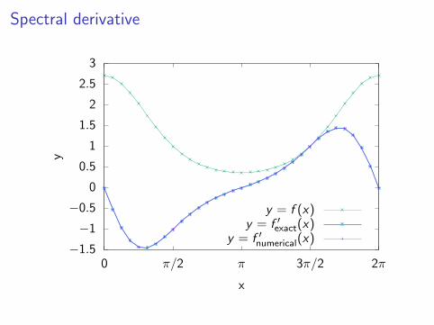
Spectral derivative

−1.5

−1

−0.5

0

0.5

1

1.5

2

2.5

3

0 π/2 π 3π/2 2π

y

x

y = f (x)y = f ′exact(x)

y = f ′numerical(x)

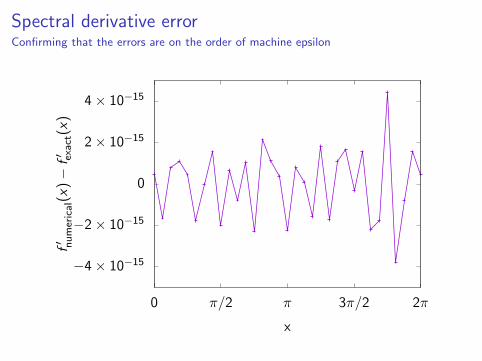
Spectral derivative errorConfirming that the errors are on the order of machine epsilon

−4× 10−15

−2× 10−15

0

2× 10−15

4× 10−15

0 π/2 π 3π/2 2π

f′ numerical(x

)−

f′ exact

(x)

x

Solving PDEs with spectral methods

Spectral methods an attractive choice for problems on periodicintervals where smooth solutions are expected. Many nonlinearwave equations have this form.

An example is the Kortweg–de Vries (KdV) equation to modelwaves on shallow water surfaces. For a function u(t, x) the KdVequation is

ut + uux + a2uxxx = 0,

where a is a constant.21

21The prefactors in front of the terms are not important, since they can bechanged by rescaling t, u, or x .

KdV equation

Computer demo: The program kdv test.cc solves the KdVequation.

It uses fourth-order Runge–Kutta method for timestepping, andspectral methods to evaluate the spatial derivatives. This giveshighly accurate solutions.

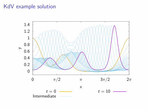
KdV example solution

0

0.2

0.4

0.6

0.8

1

1.2

1.4

0 π/2 π 3π/2 2π

y

xt = 0

Intermediatet = 10

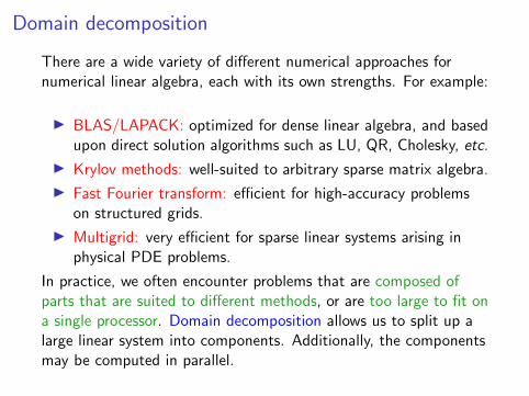
Domain decomposition

There are a wide variety of different numerical approaches fornumerical linear algebra, each with its own strengths. For example:

I BLAS/LAPACK: optimized for dense linear algebra, and basedupon direct solution algorithms such as LU, QR, Cholesky, etc.

I Krylov methods: well-suited to arbitrary sparse matrix algebra.

I Fast Fourier transform: efficient for high-accuracy problemson structured grids.

I Multigrid: very efficient for sparse linear systems arising inphysical PDE problems.

In practice, we often encounter problems that are composed ofparts that are suited to different methods, or are too large to fit ona single processor. Domain decomposition allows us to split up alarge linear system into components. Additionally, the componentsmay be computed in parallel.

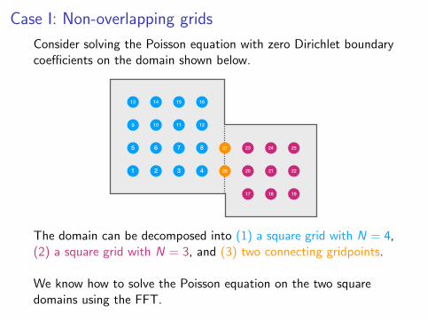
Case I: Non-overlapping grids

Consider solving the Poisson equation with zero Dirichlet boundarycoefficients on the domain shown below.

1 2 3 4

5 6 7 8

9 10 11 12

13 14 15 16

17 18 19

20 21 22

23 24 25

26

27

The domain can be decomposed into (1) a square grid with N = 4,(2) a square grid with N = 3, and (3) two connecting gridpoints.

We know how to solve the Poisson equation on the two squaredomains using the FFT.

Case I: Non-overlapping grids

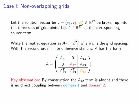
Let the solution vector be v = (v1, v2, v3) ∈ R27 be broken up intothe three sets of gridpoints. Let f ∈ R27 be the correspondingsource term.

Write the matrix equation as Av = h2f where h is the grid spacing.With the second-order finite difference stencils, A has the form

A =

A11 0 A13

0 A22 A23

AT13 AT

23 A33

.

Key observation: By construction the A12 term is absent and thereis no direct coupling between domain 1 and domain 2.

Schur complement

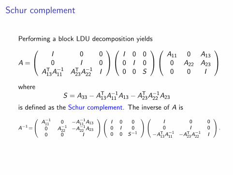
Performing a block LDU decomposition yields

A =

I 0 00 I 0

AT13A−111 AT

23A−122 I

I 0 00 I 00 0 S

A11 0 A13

0 A22 A23

0 0 I

where

S = A33 − AT13A−111 A13 − AT

23A−122 A23

is defined as the Schur complement. The inverse of A is

A−1=

A−111 0 −A−1

11 A13

0 A−122 −A−1

22 A23

0 0 I

I 0 00 I 00 0 S−1

I 0 00 I 0

−AT13A

−111 −AT

23A−122 I

.

Schur complement

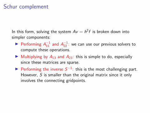
In this form, solving the system Av = h2f is broken down intosimpler components:

I Performing A−111 and A−122 : we can use our previous solvers tocompute these operations.

I Multiplying by A13 and A23: this is simple to do, especiallysince these matrices are sparse.

I Performing the inverse S−1: this is the most challenging part.However, S is smaller than the original matrix since it onlyinvolves the connecting gridpoints.

Options for inverting the Schur complement

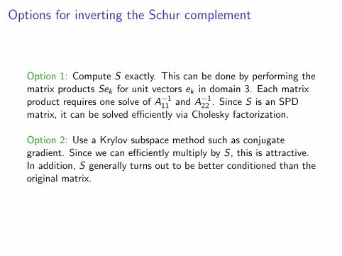
Option 1: Compute S exactly. This can be done by performing thematrix products Sek for unit vectors ek in domain 3. Each matrixproduct requires one solve of A−111 and A−122 . Since S is an SPDmatrix, it can be solved efficiently via Cholesky factorization.

Option 2: Use a Krylov subspace method such as conjugategradient. Since we can efficiently multiply by S , this is attractive.In addition, S generally turns out to be better conditioned than theoriginal matrix.

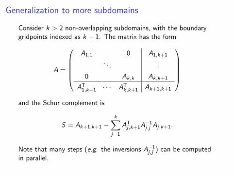
Generalization to more subdomains

Consider k > 2 non-overlapping subdomains, with the boundarygridpoints indexed as k + 1. The matrix has the form

A =

A1,1 0 A1,k+1

. . ....

0 Ak,k Ak,k+1

AT1,k+1 · · · AT

k,k+1 Ak+1,k+1

and the Schur complement is

S = Ak+1,k+1 −k∑

j=1

ATj ,k+1A

−1j ,j Aj ,k+1.

Note that many steps (e.g. the inversions A−1j ,j ) can be computedin parallel.

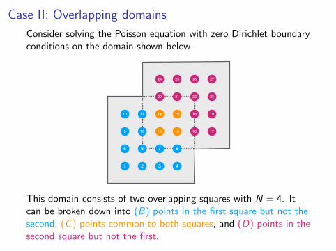
Case II: Overlapping domains

Consider solving the Poisson equation with zero Dirichlet boundaryconditions on the domain shown below.

1 2 3 4

5

9

10 19

23

25 26 27

12

14

13

15

16 17

24

6 7 8

10

11 18

21 2220

This domain consists of two overlapping squares with N = 4. Itcan be broken down into (B) points in the first square but not thesecond, (C ) points common to both squares, and (D) points in thesecond square but not the first.

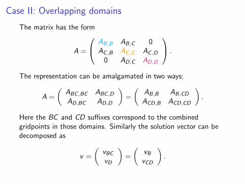
Case II: Overlapping domains

The matrix has the form

A =

AB,B AB,C 0AC ,B AC ,C AC ,D

0 AD,C AD,D

.

The representation can be amalgamated in two ways:

A =

(ABC ,BC ABC ,D

AD,BC AD,D

)=

(AB,B AB,CD

ACD,B ACD,CD

).

Here the BC and CD suffixes correspond to the combinedgridpoints in those domains. Similarly the solution vector can bedecomposed as

v =

(vBCvD

)=

(vBvCD

).

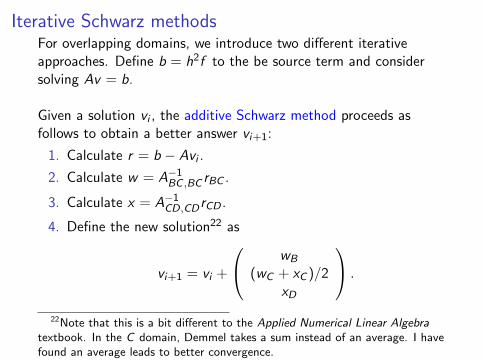
Iterative Schwarz methodsFor overlapping domains, we introduce two different iterativeapproaches. Define b = h2f to the be source term and considersolving Av = b.

Given a solution vi , the additive Schwarz method proceeds asfollows to obtain a better answer vi+1:

1. Calculate r = b − Avi .

2. Calculate w = A−1BC ,BC rBC .

3. Calculate x = A−1CD,CDrCD .

4. Define the new solution22 as

vi+1 = vi +

wB

(wC + xC )/2xD

.

22Note that this is a bit different to the Applied Numerical Linear Algebratextbook. In the C domain, Demmel takes a sum instead of an average. I havefound an average leads to better convergence.

Comments on the additive Schwarz method

Note that steps 2 and 3 can be calculated efficiently using the fastsolvers on the square grids. Steps 2 and 3 can also be done inparallel.

In step 3 of the additive Schwarz method, we use the originalresidual r from step 1, even though we have new information fromdoing the solve on the BC in step 2. This suggests a modifiedapproach.

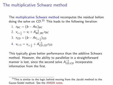
The multiplicative Schwarz method

The multiplicative Schwarz method recomputes the residual beforedoing the solve on CD.23 This leads to the following iteration:

1. rBC = (b − Avi )BC

2. vi+ 12

= vi + A−1BC ,BC rBC

3. rCD = (b − Avi+ 12)CD

4. vi+1 = vi+ 12

+ A−1CD,CDrCD

This typically gives better performance than the additive Schwarzmethod. However, the ability to parallelize in a straightforwardmanner is lost, since the second solve A−1CD,CD incorporatesinformation from the first.

23This is similar to the logic behind moving from the Jacobi method to theGauss–Seidel method. See the AM205 notes.