Embed Size (px)
Citation preview

Applied Mathematics 205
Unit IV: Nonlinear Equations and Optimization
Lecturer: Dr. David Knezevic

Unit IV: Nonlinear Equationsand Optimization
Chapter IV.3: Conditions for Optimality
2 / 41
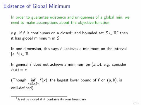
Existence of Global Minimum
In order to guarantee existence and uniqueness of a global min. weneed to make assumptions about the objective function
e.g. if f is continuous on a closed1 and bounded set S ⊂ Rn thenit has global minimum in S
In one dimension, this says f achieves a minimum on the interval[a, b] ⊂ R
In general f does not achieve a minimum on (a, b), e.g. considerf (x) = x
(Though infx∈(a,b)
f (x), the largest lower bound of f on (a, b), is
well-defined)
1A set is closed if it contains its own boundary3 / 41

Existence of Global Minimum
Another helpful concept for existence of global min. is coercivity
A continuous function f on an unbounded set S ⊂ Rn is coercive if
lim‖x‖→∞
f (x) = +∞
That is, f (x) must be large whenever ‖x‖ is large
4 / 41

Existence of Global Minimum
If f is coercive on a closed, unbounded2 set S , then f has a globalminimum in S
Proof: From the definition of coercivity, for any M ∈ R, ∃r > 0such that f (x) ≥ M for all x ∈ S where ‖x‖ ≥ r
Suppose that 0 ∈ S , and set M = f (0)
Let Y ≡ {x ∈ S : ‖x‖ ≥ r}, so that f (x) ≥ f (0) for all x ∈ Y
And we already know that f achieves a minimum (which is at mostf (0)) on the closed, bounded set {x ∈ S : ‖x‖ ≤ r}
Hence f achieves a minimum on S �
2e.g. S could be all of Rn, or a “closed strip” in Rn
5 / 41

Existence of Global Minimum
For example:
I f (x , y) = x2 + y2 is coercive on R2 (global min. at (0, 0))
I f (x) = x3 is not coercive on R (f → −∞ for x → −∞)
I f (x) = ex is not coercive on R (f → 0 for x → −∞)
Question: What about uniqueness?
6 / 41
Convexity
An important concept for uniqueness is convexity
A set S ⊂ Rn is convex if it contains the line segment between anytwo of its points
That is, S is convex if for any x , y ∈ S , we have
{θx + (1− θ)y : θ ∈ [0, 1]} ⊂ S
7 / 41
Convexity
Similarly, we define convexity of a function f : S ⊂ Rn → R
f is convex if its graph along any line segment in S is on or belowthe chord connecting the function values
i.e. f is convex if for any x , y ∈ S and any θ ∈ [0, 1], we have
f (θx + (1− θ)y) ≤ θf (x) + (1− θ)f (y)
Also, iff (θx + (1− θ)y) < θf (x) + (1− θ)f (y)
then f is strictly convex
8 / 41
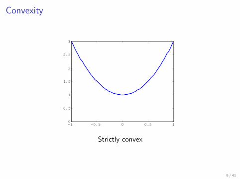
Convexity
−1 −0.5 0 0.5 10
0.5
1
1.5
2
2.5
3
Strictly convex
9 / 41

Convexity
0 0.2 0.4 0.6 0.8 1−0.1
−0.05
0
0.05
0.1
0.15
0.2
0.25
0.3
0.35
Non-convex
10 / 41

Convexity
0 0.2 0.4 0.6 0.8 10.1
0.15
0.2
0.25
0.3
0.35
0.4
0.45
0.5
Convex (not strictly convex)
11 / 41
Convexity
If f is a convex function on a convex set S , then any localminimum of f must be a global minimum
Proof: Suppose x is a local minimum, i.e. f (x) ≤ f (y) fory ∈ B(x , ε) (where B(x , ε) ≡ {y ∈ S : ‖y − x‖ ≤ ε})
Suppose that x is not a global minimum, i.e. that there existsw ∈ S such that f (w) < f (x)
(Then we will show that this gives a contradiction)
12 / 41

Convexity
Proof (continued...):
For θ ∈ [0, 1] we have f (θw + (1− θ)x) ≤ θf (w) + (1− θ)f (x)
Let σ ∈ (0, 1] be sufficiently small so that
z ≡ σw + (1− σ) x ∈ B(x , ε)
Then
f (z) ≤ σf (w) + (1− σ) f (x) < σf (x) + (1− σ) f (x) = f (x),
i.e. f (z) < f (x), which contradicts that f (x) is a local minimum!
Hence we cannot have w ∈ S such that f (w) < f (x) �
13 / 41
Convexity
Note that convexity does not guarantee uniqueness of globalminimum
e.g. a convex function can clearly have a “horizontal” section (seeearlier plot)
If f is a strictly convex function on a convex set S , then a localminimum of f is the unique global minimum
Optimization of convex functions over convex sets is called convexoptimization, which is an important subfield of optimization
14 / 41

Optimality Conditions
We have discussed existence and uniqueness of minima, buthaven’t considered how to find a minimum
The familiar optimization idea from calculus in one dimension is:set derivative to zero, check the sign of the second derivative
This can be generalized to Rn
15 / 41

Optimality Conditions
If f : Rn → R is differentiable, then the gradient vector∇f : Rn → Rn is
∇f (x) ≡
∂f (x)∂x1∂f (x)∂x2...
∂f (x)∂xn
The importance of the gradient is that ∇f points “uphill,” i.e.towards points with larger values than f (x)
And similarly −∇f points “downhill”
16 / 41
Optimality Conditions
This follows from Taylor’s theorem for f : Rn → R
Recall that
f (x + δ) = f (x) +∇f (x)T δ + H.O.T.
Let δ ≡ −ε∇f (x) for ε > 0 and suppose that ∇f (x) 6= 0, then:
f (x − ε∇f (x)) ≈ f (x)− ε∇f (x)T∇f (x) < f (x)
Also, we see from Cauchy-Schwarz that −∇f (x) is the steepestdescent direction
17 / 41

Optimality Conditions
Similarly, we see that a necessary condition for a local minimum atx∗ ∈ S is that ∇f (x∗) = 0
In this case there is no “downhill direction” at x∗
The condition ∇f (x∗) = 0 is called a first-order necessarycondition for optimality, since it only involves first derivatives
18 / 41
Optimality Conditions
x∗ ∈ S that satisfies the first-order optimality condition is called acritical point of f
But of course a critical point can be a local min., local max., orsaddle point
(Recall that a saddle point is where some directions are “downhill”and others are “uphill”, e.g. (x , y) = (0, 0) for f (x , y) = x2 − y2)
19 / 41
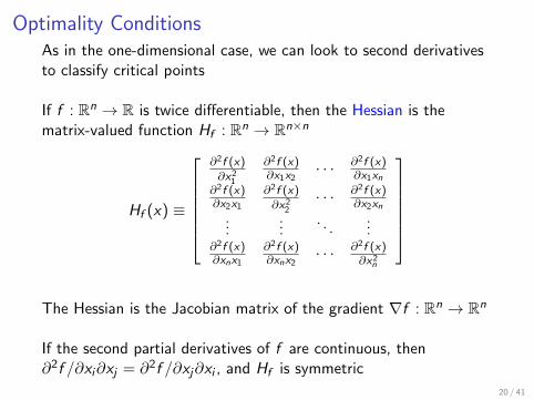
Optimality ConditionsAs in the one-dimensional case, we can look to second derivativesto classify critical points
If f : Rn → R is twice differentiable, then the Hessian is thematrix-valued function Hf : Rn → Rn×n
Hf (x) ≡
∂2f (x)∂x21
∂2f (x)∂x1x2
· · · ∂2f (x)∂x1xn
∂2f (x)∂x2x1
∂2f (x)∂x22
· · · ∂2f (x)∂x2xn
......
. . ....
∂2f (x)∂xnx1
∂2f (x)∂xnx2
· · · ∂2f (x)∂x2n
The Hessian is the Jacobian matrix of the gradient ∇f : Rn → Rn
If the second partial derivatives of f are continuous, then∂2f /∂xi∂xj = ∂2f /∂xj∂xi , and Hf is symmetric
20 / 41
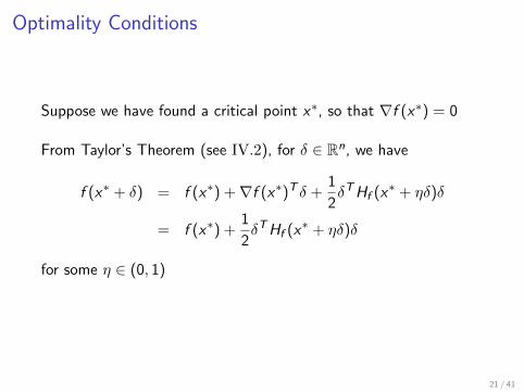
Optimality Conditions
Suppose we have found a critical point x∗, so that ∇f (x∗) = 0
From Taylor’s Theorem (see IV.2), for δ ∈ Rn, we have
f (x∗ + δ) = f (x∗) +∇f (x∗)T δ +1
2δTHf (x∗ + ηδ)δ
= f (x∗) +1
2δTHf (x∗ + ηδ)δ
for some η ∈ (0, 1)
21 / 41

Optimality Conditions
Recall positive definiteness: A is positive definite if xTAx > 0
Suppose Hf (x∗) is positive definite
Then (by continuity) Hf (x∗ + ηδ) is also positive definite for ‖δ‖sufficiently small, so that: δTHf (x∗ + ηδ)δ > 0
Hence, we have f (x∗ + δ) > f (x) for ‖δ‖ sufficiently small, i.e.f (x∗) is a local minimum
Hence, in general, positive definiteness of Hf at a critical point x∗
is a second-order sufficient condition for a local minimum
22 / 41

Optimality Conditions
A matrix can also be negative definite: xTAx < 0 for all x 6= 0
Or indefinite: There exists x , y such that xTAx < 0 < yTAy
Then we can classify critical points as follows:
I Hf (x∗) positive definite =⇒ x∗ is a local minimum
I Hf (x∗) negative definite =⇒ x∗ is a local maximum
I Hf (x∗) indefinite =⇒ x∗ is a saddle point
23 / 41

Optimality Conditions
Also, positive definiteness of the Hessian is closely related toconvexity of f
If Hf (x) is positive definite, then f is convex on some convexneighborhood of x
If Hf (x) is positive definite for all x ∈ S , where S is a convex set,then f is convex on S
Question: How do we test for positive definiteness?
24 / 41

Optimality Conditions
Answer: A is positive (resp. negative) definite if and only if alleigenvalues of A are positive (resp. negative)3
Also, a matrix with positive and negative eigenvalues is indefinite
Hence we can compute all the eigenvalues of A and check theirsigns
3This is related to the Rayleigh quotient, see Unit V25 / 41
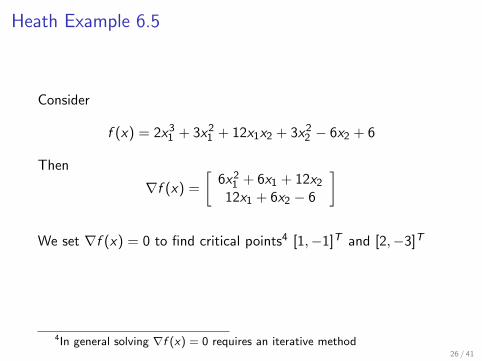
Heath Example 6.5
Consider
f (x) = 2x31 + 3x21 + 12x1x2 + 3x22 − 6x2 + 6
Then
∇f (x) =
[6x21 + 6x1 + 12x2
12x1 + 6x2 − 6
]
We set ∇f (x) = 0 to find critical points4 [1,−1]T and [2,−3]T
4In general solving ∇f (x) = 0 requires an iterative method26 / 41

Heath Example 6.5, continued...
The Hessian is
Hf (x) =
[12x1 + 6 12
12 6
]and hence
Hf (1,−1) =
[18 1212 6
], which has eigenvalues 25.4,−1.4
Hf (2,−3) =
[30 1212 6
], which has eigenvalues 35.0, 1.0
Hence [2,−3]T is a local min. whereas [1,−1]T is a saddle point
27 / 41

Optimality Conditions: Equality Constrained Case
So far we have ignored constraints
Let us now consider equality constrained optimization
minx∈Rn
f (x) subject to g(x) = 0,
where f : Rn → R and g : Rn → Rm, with m ≤ n
Since g maps to Rm, we have m constraints
This situation is treated with Lagrange mutlipliers
28 / 41

Optimality Conditions: Equality Constrained Case
We illustrate the concept of Lagrange multipliers for f , g : R2 → R
Let f (x , y) = x + y and g(x , y) = 2x2 + y2 − 5
−3 −2 −1 0 1 2 3
−2
−1.5
−1
−0.5
0
0.5
1
1.5
2
At any x ∈ S we must move in direction (∇g(x))⊥ to remain in S ,hence (∇g(x))⊥ is tangent direction5 (and ∇g(x) is normal to S)
5This follows from Taylor’s Theorem: g(x + δ) ≈ g(x) +∇g(x)T δ29 / 41

Optimality Conditions: Equality Constrained Case
Also, change in f due to infinitesimal step in direction (∇g(x))⊥ is
f (x ± ε(∇g(x))⊥) = f (x)± ε∇f (x)T (∇g(x))⊥ + H.O.T.
Hence stationary point x∗ ∈ S if ∇f (x∗)T (∇g(x∗))⊥ = 0, or
∇f (x∗) = λ∗∇g(x∗), for some λ∗ ∈ R
−3 −2 −1 0 1 2 3
−2
−1.5
−1
−0.5
0
0.5
1
1.5
2
30 / 41

Optimality Conditions: Equality Constrained Case
This shows that for a stationary point with one constraint, ∇fmust be orthogonal to the “tangent direction” of S
Now, consider the case with m > 1 equality constraints
Then g : Rn → Rm and we now have a set of constraint gradientvectors, ∇gi , i = 1, . . . ,m
Then we have S = {x ∈ Rn : gi (x) = 0, i = 1, . . . ,m}
Any “tangent direction” at x ∈ S must be orthogonal to allgradient vectors {∇gi (x), i = 1, . . . ,m} to remain in S
31 / 41

Optimality Conditions: Equality Constrained Case
Let T (x) ≡ {v ∈ Rn : ∇gi (x)T v = 0, i = 1, 2, . . . ,m} denote theorthogonal complement of span{∇gi (x), i = 1, . . . ,m}
Then, for δ ∈ T (x) and ε ∈ R>0, εδ is a step in a “tangentdirection” of S at x
Since we have
f (x∗ + εδ) = f (x∗) + ε∇f (x∗)T δ + H.O.T.
it follows that for a stationary point we need ∇f (x∗)T δ = 0 for allδ ∈ T (x∗)
Hence at a stationary point x∗ ∈ S , ∇f (x∗) must be in theorthogonal complement of T (x∗)!
32 / 41
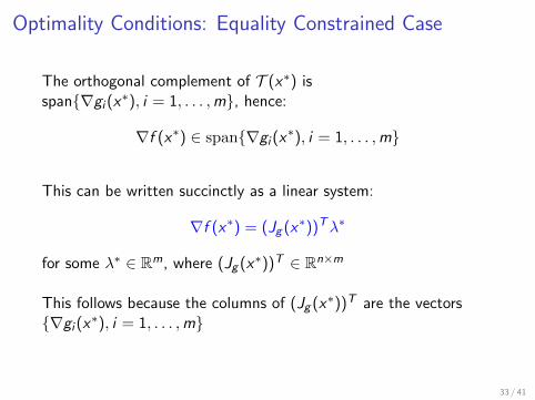
Optimality Conditions: Equality Constrained Case
The orthogonal complement of T (x∗) isspan{∇gi (x∗), i = 1, . . . ,m}, hence:
∇f (x∗) ∈ span{∇gi (x∗), i = 1, . . . ,m}
This can be written succinctly as a linear system:
∇f (x∗) = (Jg (x∗))Tλ∗
for some λ∗ ∈ Rm, where (Jg (x∗))T ∈ Rn×m
This follows because the columns of (Jg (x∗))T are the vectors{∇gi (x∗), i = 1, . . . ,m}
33 / 41

Optimality Conditions: Equality Constrained Case
We can write equality constrained optimization problems moresuccinctly by introducing the Lagrangian function, L : Rn+m → R,
L(x , λ) ≡ f (x) + λTg(x)
= f (x) + λ1g1(x) + · · ·+ λmgm(x)
Then we have,
∂L(x ,λ)∂xi
= ∂f (x)∂xi
+ λ1∂g1(x)∂xi
+ · · ·+ λn∂gn(x)∂xi
, i = 1, . . . , n
∂L(x ,λ)∂λi
= gi (x), i = 1, . . . ,m
34 / 41

Optimality Conditions: Equality Constrained Case
Hence
∇L(x , λ) =
[∇xL(x , λ)∇λL(x , λ)
]=
[∇f (x) + Jg (x)Tλ
g(x)
],
so that the first order necessary condition for optimality for theconstrained problem can be written as a nonlinear system:6
∇L(x , λ) =
[∇f (x) + Jg (x)Tλ
g(x)
]= 0
(As before, stationary points can be classified by considering theHessian, though we will not consider this here...)
6n +m variables, n +m equations35 / 41

Optimality Conditions: Equality Constrained Case
See Lecture: Constrained optimization of cylinder surface area
36 / 41

Optimality Conditions: Equality Constrained Case
As another example of equality constrained optimization, recall ourunderdetermined linear least squares problem from I.3
minb∈Rn
f (b) subject to g(b) = 0,
where f (b) ≡ bTb, g(b) ≡ Ab − y and A ∈ Rm×n with m < n
37 / 41
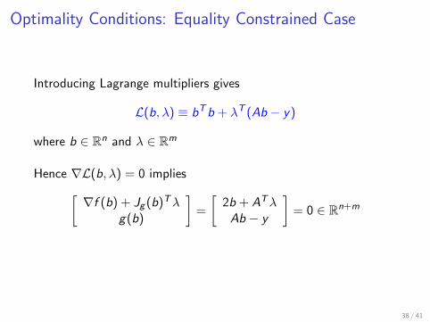
Optimality Conditions: Equality Constrained Case
Introducing Lagrange multipliers gives
L(b, λ) ≡ bTb + λT (Ab − y)
where b ∈ Rn and λ ∈ Rm
Hence ∇L(b, λ) = 0 implies[∇f (b) + Jg (b)Tλ
g(b)
]=
[2b + ATλAb − y
]= 0 ∈ Rn+m
38 / 41

Optimality Conditions: Equality Constrained Case
Hence, we obtain the (n + m)× (n + m) square linear system[2I AT
A 0
] [bλ
]=
[0y
]
We can solve this system analytically for
[bλ
]∈ Rn+m
39 / 41

Optimality Conditions: Equality Constrained Case
We have b = −12A
Tλ from the first “block row”
Subsituting into Ab = y (the second “block row”) yieldsλ = −2(AAT )−1y
And hence
b = −1
2ATλ = AT (AAT )−1y
which was the solution we introduced (but didn’t derive) in I.3
40 / 41

Optimality Conditions: Inequality Constrained Case
Similar Lagrange multiplier methods can be developed for the moredifficult case of inequality constrained optimization
However, this is outside the scope of AM205...
...though we will use Matlab’s functions for inequality constrainedoptimization
41 / 41


![Nonlinear Panel Models with Interactive Effects · 2018-09-21 · arXiv:1412.5647v1 [stat.ME] 17 Dec 2014 Nonlinear Panel Models with Interactive Effects∗ Mingli Chen ‡Iv´an](https://img.pdfslide.us/doc/110x75/5ec93352fabef3665e12c01c/nonlinear-panel-models-with-interactive-eiects-2018-09-21-arxiv14125647v1.jpg)