Embed Size (px)
Citation preview
Applied Mathematical Modelling 40 (2016) 542–564
Contents lists available at ScienceDirect
Applied Mathematical Modelling
journal homepage: www.elsevier .com/locate /apm
Simulation of three-dimensional cavitation behind a disk usingvarious turbulence and mass transfer models
http://dx.doi.org/10.1016/j.apm.2015.06.0020307-904X/� 2015 Elsevier Inc. All rights reserved.
⇑ Corresponding author. Tel.: +98 (51) 38805136; fax: +98 (511) 8763304.E-mail address: [email protected] (E. Roohi).
Ehsan Roohi ⇑, Mohammad-Reza Pendar, Amin RahimiHigh Performance Computing (HPC) Laboratory, Department of Mechanical Engineering, Faculty of Engineering, Ferdowsi University of Mashhad, P.O.Box 91775-1111, Mashhad, Iran
a r t i c l e i n f o
Article history:Received 29 March 2014Received in revised form 9 June 2015Accepted 23 June 2015Available online 2 July 2015
Keywords:Disk cavitatorLES turbulence modelMass transfer modelOpenFOAMVolume of fluid (VOF)Zwart model
a b s t r a c t
In this study, we performed numerical investigations of the cavitating and supercavitatingflow behind a three-dimensional disk with a particular emphasis on detailed comparisonsof various turbulence and mass transfer models. Simulations were performed using theOpenFOAM package and flows at three different cavitation numbers, (r = 0.2, 0.1, and0.05) were considered. Large eddy simulation (LES) and k—x shear stress transport turbu-lence approaches were coupled with various mass transfer model types (e.g., Kunz,Schnerr–Sauer, and Zwart models). The Zwart mass transfer model was added to the stan-dard OpenFOAM package. A compressive volume of fluid method was used to track theinterface between the liquid and vapor phases. Our numerical results in terms of the cavitylength, diameter, and drag coefficient compared fairly well with experimental data and abroad set of analytical relations. Moreover, this study provides a better understanding ofthe cavitation dynamics behind disk cavitators. Our results indicate that the most accuratesolutions will be obtained by applying an LES turbulence approach combined with theKunz mass transfer model.
� 2015 Elsevier Inc. All rights reserved.
1. Introduction
Cavitation is a multi-phase and complex physical phenomenon, which occurs when the local liquid pressure becomeslower than its saturated vapor pressure [1]. This phenomenon appears often over marine vehicle applications such as sub-marines and marine propeller blades. To increase the performance of submarines by reducing viscous drag, underwater vehi-cles usually operate in cavitating conditions [2].
Cavitation is an unsteady, three-dimensional (3-D), and discontinuous or periodic phenomenon, which occurs during theformation, growth, and rapid collapse of bubbles [3]. A dimensionless number characterizes this process, i.e.,r ¼ ðP1 � P#Þ=0:5qU2
1, which is called the cavitation number [1]. If the moving body is accelerated to high speeds, supercav-itation will occur, which refers to a long cavity that extends more than the body length and that closes in the liquid. There is aconstant movement of a re-entrant liquid jet in the cavity closure section.
Studying the cavitating flow behind a 3-D disk cavitator has been an interest of the scientific community in this field formany years. Challenging issues that need to be considered during the numerical simulation of a 3-D cavitation are: the
Nomenclature
Ae, Al parameters in near wall length scalesB unresolved transport term in LESCe, CK LES empirical constant coefficientsCd drag coefficientCl parameter in near wall length scalesCDKx positive portion of the cross-diffusionCdest, Cprod Kunz mass transfer model constantsCd0 constant in the drag coefficient for a disk cavitatorCc constant between 0 and 1Co courant number (C = U � dt/dx)D cavity diameterd cavitator diameterD rate of strain tensor~DD eddy diffusivity tensorE constant coefficientFe, Fc Zwart two empirical coefficientsF1 turbulence Function (given by Eq. (15))G filter functionI unit tensorI turbulent intensityk kinetic energyL cavity lengthl liquidll, le near wall length scalesL characteristic length (disk diameter)d turbulence length scale_m mass transfer rate between the phases
n0 initial number of bubblesp pressureRe Reynolds numberRb radius of bubblesRB radius of a nucleation siternuc nucleation site volume fractionS viscous stress tensorS strain rateus friction velocitymSGS subgrid scale viscosityt1 mean flow timeU velocity magnitudeuþ non-dimensional velocityXj components of the Cartesian coordinatey distance between surfacesyw wall distanceyþ non-dimensional wall distancer cavitation number1 free stream value/ volumetric fluxj Von Karman Constantv velocity vector# vaporq densitys wall shear stressx specific dissipation ratel viscosityD filter widthc volume fractionsij shear stress tensor
E. Roohi et al. / Applied Mathematical Modelling 40 (2016) 542–564 543
lk viscosity of the vortexb�; rx2; a; b; cl constant coefficients for the k–x SST turbulence modellog logarithmic regionvis viscous regionw wall– averaging
544 E. Roohi et al. / Applied Mathematical Modelling 40 (2016) 542–564
selection of an appropriate mass transfer model, a technique for solving the advection equation of the free surface, and theapplication of an appropriate turbulence model.
Kunz et al. [4], Singhal et al. [5], and Merkle et al. [6] proposed semi-analytical mass transfer models for cavitation. Sauer[7] and Yuan et al. [8] suggested a cavitation mass transfer model with some changes and improvements based on the clas-sical Rayleigh equation. Zwart et al. [9] derived a mass transfer model based on the simplified Rayleigh-Plesset equation,which was divided into two parts: one for the liquid phase condensation and another for the vapor phase production.Senocak and Shyy [10] suggested an analytical model based on the balance of mass–momentum around the cavity interface.Chen et al. [11] applied a computer code including several homogenous-equilibrium cavitation models and a local linear k–eturbulence model to consider cavitation around a disk cavitator. The cavity shape and profiles were found to agree well withthe analytical solutions and an experimental relation over a broad range of cavitation numbers. Typically, the volume of fluid(VOF) technique is utilized to solve the advection equation of the liquid volume fraction and to predict the cavity interfaceaccurately. The VOF technique has been shown to be an appropriate tool for the numerical simulation of free-surface flows[12]. VOF can capture the cavity shape and track the cavity interface in an accurate manner. A review of the literature showsthat VOF has been employed extensively for treating this class of problems [13–17]. Shang [13], Passandideh-Fard and Roohi[14], Frobenius and Schilling [15], Wiesche [16], and Bouziad et al. [17] all used the VOF method to simulate cavitation overvarious geometries.
Cavitating flows occur under highly unsteady conditions at large Reynolds number. Thus, the selection of an appropriateturbulence model is one of the essential issues that must be addressed to achieve an accurate treatment of cavitation.Various approaches such as the large eddy simulation (LES) and k–x shear stress transport (SST) turbulence model have beenutilized to incorporate turbulence effects in cavitating flows [3,18–21]. Compared with other turbulence models, LES canestimate the details of small-scale flow structures in cavitating flows with better fidelity.
Kunz et al. [22] developed a cavitation model based on multiphase computational fluid dynamics and they examined thevalidity of the model for the flow around submerged axisymmetric objects with steady and transient natural cavitation.Numerical predictions showed that the pressure distribution, drag coefficient, and cavity shape agreed well with experimen-tal data. Passandideh-Fard and Roohi [14] performed transient two-dimensional (2-D)/axisymmetric simulations of the cav-itating flows behind disk and cone cavitators. Nouri et al. [23] used the finite volume technique to simulate the developingcavitation behind a disk with the Kunz cavitation model and by considering LES as the turbulence model. They comparedtheir computational results with experimental data and the accuracy of their results demonstrated the capacity of combinedcavitation and turbulence models for predicting cavity characteristics. Baradaran-Fard and Nikseresht [24] simulated theunsteady 3-D cavitating flows around a circular disk and a cone cavitator. Reynolds Averaged Navier–Stokes (RANS) equa-tions and an additional transport equation for the liquid volume fraction were solved using the finite volume approachtogether with the Semi-Implicit Method for Pressure Linked Equations (SIMPLE) algorithm. A k–x SST model was usedfor modeling turbulent flows and the results agreed well with experimental data and analytical relations. In contrast to[23,24], the present study uses 3-D simulations with a much more accurate numerical model, i.e., the VOF algorithm, as wellas various sets for cavitation and advanced turbulence models. Guo et al. [25] simulated the cavitating flow around an under-water projectile with natural and ventilated cavitation based on the homogeneous equilibrium flow model, a mixture modelfor the transport equation, and a local linear low-Reynolds number k–e turbulence model. They showed that the morphologyof the ventilated cavity was similar to that of the natural cavity at the same cavitation number, except at the tail of the cavity.Shang et al. [26] validated numerical simulations of the cavitating flow over a sphere based on experimental data. Roohi et al.[27] used the LES turbulence approach to investigate the cavitating flows over hydrofoils at various cavitation numbers usingthe OpenFOAM package. Morgut et al. [28] compared the Kunz, Zwart, and Full Cavitation Model mass transfer models usingRANS turbulence equations over a hydrofoil. Shang [13] simulated cavitation around cylindrical objects such as a submarinewithin wide ranges of cavitation numbers from 0.2 to 1.0, where the k–x SST turbulence model, VOF method, and Sauermass transfer model were employed to capture the cavitation mechanisms. Ji et al. [29–31] used the LES turbulenceapproach and Sauer mass transfer model to investigate the flow characteristics over various types of hydrofoils.
In this study, we validated the ability of the open source package OpenFOAM to simulate the cavitation and supercavi-tation flow behind a disk cavitator, for which experimental and analytical data are widely available [2]. The VOF techniqueis employed to track the interface between the liquid and vapor phases. The VOF model implemented in OpenFOAM consid-ers the effect of the surface tension force over the free surface. Both the LES and k–x SST turbulence model are used to sim-ulate the cavitating flows behind the disk. Furthermore, we compare our results with those obtained using the Kunz, Sauer,and Zwart mass transfer models. In contrast to previous studies that focused on cavitation behind a disk, no 3-D simulations
E. Roohi et al. / Applied Mathematical Modelling 40 (2016) 542–564 545
have been reported for disk cavitation simulations based on the combination of accurate surface reconstruction by VOF,highly accurate turbulence models such as k–x SST and LES, and a comprehensive set of cavitation models, i.e., Kunz,Sauer, and Zwart. In addition, we provide detailed comparisons of the results obtained using the aforementioned turbulenceand mass transfer models, which have not been reported in previous studies.
2. Mathematical model
2.1. Governing equations
The governing continuity and momentum equations for a homogeneous mixture multiphase flow are given as:
@tðqvÞ þ r � ðqv � vÞ ¼ �rpþr � s;@tqþr � ðqvÞ ¼ 0:
ð1Þ
The rate-of-strain tensor is expressed as:
D ¼ 12ðrv þrvTÞ: ð2Þ
A phase change from liquid to vapor occurs under cavitation, so multiphase flow modeling should be employed todescribe the flow. In this study, we consider a ‘‘two-phase mixture’’ method, which uses a local vapor volume frac-tion transport equation and source terms for the mass transfer rate between the two phases due to cavitation, asfollows:
@tc# þr � ðc#mÞ ¼ _m; ð3Þ
where _m is the mass transfer rate between the phases. The mixture density q and the viscosity l are defined asfollows:
l ¼ clll þ ð1� clÞl#; ð4Þ
q ¼ qlcl þ ð1� clÞq#; ð5Þ
where the subscripts l and # indicate the liquid and vapor phases, respectively.
2.2. Mass transfer modeling
We utilized three different mass transfer models in the current study, i.e., Kunz, Schnerr–Sauer, and Zwart. Thesemi-analytical cavitation model proposed by Kunz et al. [4] is implemented in the standard OpenFOAM package [32]. In thismodel, there are two different source terms for vaporization and condensation (i.e., bubble growth and collapse) during cav-itation as follows:
@c#@tþ ~r � ðc#�vÞ ¼ Cprodq#MinðP � P#;0Þc#
qlð0:5qlu21Þt1
� Cdestð1� c#Þc2#
qlt1
MaxðP � P#;0ÞjP � P#j
: ð6Þ
The Kunz model assumes a moderate rate of constant condensation to reconstruct cavitation with a suitable accuracy.Cdest and Cprod are two empirical coefficients, the values of which were set to 1000 and 75, respectively, to ensure the bestoverall agreement with the experimental data obtained from various geometries [27]. The characteristic time (mean flowtime) is defined as t1 = Dcavitator/U1, where Dcavitator is the diameter of the cavitator and U1 is the free-stream velocity. Pl
and P# are the liquid pressure and vapor pressure, respectively. The Kunz model predicts the cavity region quite accurately,especially in the closure area, where this is a continuous flow of the re-entrant liquid jet and detachment of small vaporstructures from the cavity cloud [27].
A mass transfer model was derived by Schnerr–Sauer, as follows [33].
@c#@tþ ~r � ðc#�vÞ ¼ q#ql
qð1� c#Þc#
3Rb
ffiffiffiffiffiffiffiffiffiffiffiffiffiffiffiffiffiffiffiffiffi23jp# � pj
ql
s: ð7Þ
This model is a function of the bubble diameter and bubble numbers per volume unit. In Eq. (7), Rb is the radius of thebubbles and it is assumed to be a function of the vapor volume fraction, which can be expressed as follows:
Rb ¼3
4pn0
c#1� c#
� �13
: ð8Þ
546 E. Roohi et al. / Applied Mathematical Modelling 40 (2016) 542–564
The Schnerr–Sauer model is based on the Rayleigh–Plesset equation and it requires the estimation of the initial number ofbubbles (n0), the value of which was set to 1.6 � 109 [32]. Our literature review showed that there is not a unique value for n0
(see [8,15]). In fact, this parameter is adjusted by comparing the numerical results with experimental data or analytical solu-tions of cavitating flows. In this study, we used the default value in the OpenFOAM package for n0. Schnerr–Sauer solutionsagree well with analytical solutions for cavity parameters using this default value (see Section 4.3). According to Eq. (8), thebubble radius is a function of the local vapor volume fraction at each location. This model ignores bubble interactions,non-spherical bubble geometries, and local mass–momentum transfer.
The cavitation model suggested by Zwart et al. is governed by the following mass transfer equation [9]:
_m ¼�Fe 3rnucð1�c#Þq#
RB
ffiffiffiffiffiffiffiffiffiffiffiffi2ðP#�PÞ
3ql
qP < P#;
Fc 3c#q#RB
ffiffiffiffiffiffiffiffiffiffiffiffi2ðP�P#Þ
3ql
qP > P#;
8><>: ð9Þ
where rnuc is the nucleation site volume fraction, RB is the radius of a nucleation site, and Fe and Fc are two empirical coef-ficients for the evaporation and condensation processes, respectively. According to [9], by default, the aforementioned coef-ficients are set as: rnuc = 5.0 � 10�4, RB = 1.0 � 10�6, Fe = 50, Fc = 0.01. This model is based on the simplified Rayleigh–Plessetequation for bubble dynamics [28]. In the above equation, the expressions for condensation and evaporation terms are notsymmetric, and thus for evaporation, c# is replaced by rnucð1� c#Þ, which indicates that the nucleation site density decreasesas the vapor volume fraction increases.
2.3. The k–x SST turbulence model
We used the k–x SST model as one of the turbulence models. Menter [34] developed the k—x SST model to efficientlyblend the accurate formulation of the k—x model in the near-wall region and the k—e model at the far field. In this model,the turbulence kinetic energy and specific dissipation rate, respectively, are given as follows:
@
@tðqkÞ þ @
@xjðqkujÞ ¼
@
@xjlþ lt
rk3
� �@k@xj
� �þ sij
@ui
@xj� b�qkx; ð10Þ
@ðqxÞ@t
þ @ðqujxÞ@xj
¼ @
@xjlþ lt
rx3
� �@x@xj
� �þx
ka3sij
@ui
@xj
� �� b3qx2 þ ð1� F1Þ2q
1xrx2
@k@xj
@x@xj
: ð11Þ
The model coefficients ða3; b3;rk3;rx3Þ are linear combinations of the corresponding coefficients of k—x and modifiedk—e turbulence models, which are calculated as follows:
w ¼ F1wkx þ ð1� F1Þwke; a3 ¼ F1a1 þ ð1� F1Þa2; ð12Þ
k—x : a1 ¼ 5=9; b1 ¼ 3=40; rk1 ¼ 2; rx1 ¼ 2; b� ¼ 9=100k—e : a2 ¼ 0:44; b2 ¼ 0:0828; rk2 ¼ 1; rx2 ¼ 1=0:856; Cl ¼ 0:09
sij ¼ lt 2sij �23@uk
@xkdij
� �� 2
3qkdij ð13Þ
S ¼ffiffiffiffiffiffiffiffiffiffiffi2sijsij
q; sij ¼
12
@ui
@xjþ @uj
@xi
� �; ð14Þ
where S denotes the magnitude of the strain rate and sij is the strain rate tensor.
F1 ¼ tanhðC4Þ; ð15Þ
C ¼min max
ffiffiffikp
b�xy;500mxy2
!;4qrx2kCDKxy2
!; ð16Þ
where y is the distance to the next surface and CDKx is the positive portion of the cross-diffusion term of Eq. (11):
CDKx ¼max 2qrx21x
@k@xj
@x@xj
;10�20� �
: ð17Þ
This model benefits from the Wilcox k—x and the superiority of the Launder–Spalding k—e model, but it cannot predictthe starting point and the amount of flow separation from smooth surfaces due to the over-prediction of the eddy-viscosity,i.e., the transport of the turbulence shear stress is not considered properly. By adding a limiter to the formulation of theeddy-viscosity, an appropriate transport behavior can be obtained:
E. Roohi et al. / Applied Mathematical Modelling 40 (2016) 542–564 547
lt ¼ qk
maxðx; SF2Þ; ð18Þ
where S is an invariant measure of the strain rate and F2 is a blending function, as follows:
F2 ¼ tanhðC22Þ; ð19Þ
with the function C2 as:
C2 ¼max2ffiffiffikp
b�xy;500mxy2
!: ð20Þ
If the underlying assumptions do not hold for the free shear flow, F2 restricts the limiter to the wall boundary layer.Following Menter et al. [35], OpenFOAM uses a blending function that depends on y+ for the near-wall treatment. The
solutions for x in the linear and the logarithmic near-wall region are as follows:
xlog ¼1
0:3jus
y; xVis ¼
6m0:075y2 : ð21Þ
The equations above are rewritten in terms of y+ to obtain a smooth blending function.
x1ðyþÞ ¼ffiffiffiffiffiffiffiffiffiffiffiffiffiffiffiffiffiffiffiffiffiffiffiffiffiffiffiffiffiffiffiffiffiffiffiffiffiffiffiffiffix2
VisðyþÞ þx2logðyþÞ
q: ð22Þ
A similar formulation is used for the velocity near the wall.
uViss ¼
U1
yþ; ulog
s ¼U1
1j lnðyþÞ þ c
; ð23Þ
us ¼ffiffiffiffiffiffiffiffiffiffiffiffiffiffiffiffiffiffiffiffiffiffiffiffiffiffiffiffiffiffiffiffiffiffiffiuVis
s� �4 þ ulog
s
� �44
r: ð24Þ
This formulation expresses the relation between the velocity near the wall and the wall shear stress. A zero flux boundarycondition is applied for the k-equation, which is correct for both the low-Re and the logarithmic limit. This model exploitsthe robust near wall formulation of the underlying k–x model and switches automatically from a low-Reynolds number for-mulation to a wall function treatment based on the grid density [35].
2.4. Large eddy simulation
The LES turbulence approach is based on computing the large, energy-containing structures that are resolved on the com-putational grid while the smaller sub-grid eddies are modeled. RANS models are based on solving an ensemble average of theflow properties, but LES typically allows for medium to small scale, transient flow structures. The cavitating flows areunsteady, so this feature of the LES is an important property that helps to capture the mechanisms that govern the dynamicsof the formation and shedding of the cavity [36–38]. The LES equations are theoretically derived from Eq. (1) [39]. In the
ordinary LES, all of the variables, i.e., f, are split into grid scale (GS) and subgrid scale (SGS) components, i.e., f ¼ f þ f 0, where�f ¼ G � f is the GS component, G = G(X, D) is the filter function, and D = D(x) is the filter width [40].
OpenFOAM utilizes the top-hat filter as follows [41]:
Gðx;DÞ ¼1D : if x 6 D
2
� �;
0 : otherwise:
(ð25Þ
In OpenFOAM, the filter width D is set as equal to the grid spacing [41]. The top-hat (box) filter is an implicit filter thatdepends on the grid spacing, which in turn determines that the smallest scales are retained. All of the scales are modeledbelow the filter width D, the SGS. In this study, we used ‘‘smooth’’ delta, as described below.
After the fluid moves from a coarse mesh area into a fine mesh area, or vice versa, an unphysical non-equilibriumstate will exist for finite levels of resolved and unresolved turbulence [41]. Eddies that move from a coarse mesh toa finer mesh will be resolved more accurately on the finer grid, but the SGS turbulent length scale is directly relatedto the cell size, which is the same as the filter size, so there will be an abrupt decrease in the SGS viscosity.OpenFOAM applies smoothing to the distribution of the SGS turbulent length scale (or filter width D) near the gridrefinement boundaries to alleviate this problem, i.e., D is smoothed using a biased wave scheme [41]. This schemesmoothes the distribution by increasing the SGS length scale for cells that neighbor larger cells, so the value of D cannotbe smaller than the cell-derived value (see Fig. 1). The gradient of the smoothed distribution is fixed by an adaptablecoefficient, CDs, as follows:
D ¼maxðDP ;DN=CDSÞ; ð26Þ
Fig. 1. Schematic showing the distribution of a smoothed filter width on a typical one-dimensional mesh [41].
548 E. Roohi et al. / Applied Mathematical Modelling 40 (2016) 542–564
where P and N denote the current cell and the neighbor cell, respectively. In practice, the value of CDS � 1.15 is set so theequilibrium is obtained over 4–5 cells from the refinement boundary [42].
The LES equations, which are obtained after convolving the continuity and momentum equations, by the G = G(x, D) fil-tering, can be expressed as:
@tðqvÞ þ r:ðqv � vÞ ¼ �rpþr:ðs� BÞ;@tqþr:ðqvÞ ¼ 0;
ð27Þ
where the rate-of-strain tensor is expressed as D ¼ 12 ðrv þrvTÞ. B is the unresolved transport term, which can be decom-
posed exactly as [43]:
B ¼ q � v � v � v � v þ ~B� �
; ð28Þ
where ~B needs to be modeled. The most common subgrid modeling approaches utilize an eddy or subgrid viscosity, mSGS,where mSGS can be computed with a wide variety of methods. In eddy-viscosity models,
B ¼ 23
�qkI � 2lk~DD; ð29Þ
where k is the SGS kinetic energy, l is the SGS eddy viscosity, and ~DD is the SGS eddy diffusivity. In the current study, SGSterms are modeled using the one equation eddy-viscosity model (OEEVM). In order to obtain k, the OEEVM uses the follow-ing equation:
@ð�qkÞ@tþr:ð�qk~vÞ ¼ �B:~Dþr:ðlrkÞ þ �qe; ð30Þ
e ¼ cek3=2=D; ð31Þ
lk ¼ ck �qDffiffiffikp
; ð32Þ
where Ce and Ck are both empirical constant coefficients, which are set as 1.048 and 0.094, respectively, in the OpenFOAMpackage.
In low-Reynolds number regions near walls, OpenFOAM applies Wolfshtein’s wall damping model to these equations toensure the correct near-wall treatment [41]. This model employs Eqs. (31) and (32), but it replaces the length scale:
e ¼ cek3=2=le; ð33Þ
lk ¼ ck �qllffiffiffikp
; ð34Þ
where the length scales le and ll include the necessary damping effects in the near-wall region in terms of viscous wall units,as follows:
le ¼ Cl yw 1� e�yþ=Aeh i
; ð35Þ
ll ¼ Cl yw 1� e�yþ=Alh i
; ð36Þ
where Cl ¼ jC3=4l , Al = 20–30, Ae = 2Cl [41].
It should be noted after we compared the computational costs of OEEVM with the most popular SGS model, i.e.,Smagorinsky, we found that the computational costs decreased by up to 30%. However, it should also be noted that because
E. Roohi et al. / Applied Mathematical Modelling 40 (2016) 542–564 549
there are no experimental pictures of the cavity shape to compare the vapor shedding, fluctuating cavity behavior, or reen-trant jet with the numerical solutions obtained from the OEEVM or Smagorinsky SGS models, then it is appropriate to use amore accurate SGC approach, although it incurs higher computational costs. By contrast, if the aim of computation is to com-pare the general properties of the cavity cloud such as the length, diameter, and pressure drag coefficient, then the simula-tion should be performed with less expensive SGS models because these parameters are insensitive to the SGS modelemployed.
A blending function is employed in OpenFOAM’s LES to manage different values of y+ for the first grid cell and its influenceon the near-wall function selection [41,44]. The blending function is given by Spalding Law as follows [41]:
yþ ¼ uþ1E
ejuþ � 1� juþ � 12ðjuþÞ2 � 1
6ðjuþÞ3
; ð37Þ
where j = 0.4187, E = 9, yþ ¼ yus=m, and uþ ¼ u=us. The main advantage of using this unified wall function is that the firstoff-the-wall grid point can be located in the buffer or viscous regions (y+ < 30) without the loss of accuracy that is inherentin the logarithmic profiles, which limit validity [41].
2.5. Volume of fluid model
In this study, the VOF method [45] is adapted to capture the interface between the liquid and vapor phases. c1 is the vol-ume fraction of fluid 1 defined by the following for:
c1 ¼1 fluid 10 fluid 20 < c1 < 1 at the interface
8><>: ð38Þ
Assuming that the two fluids are incompressible, the transport equations of each volume fraction c1 and c2 are given asfollows:
@ci
@tþ ~r � ðv iciÞ ¼ 0; i ¼ 1; 2: ð39Þ
It is sufficient to only consider the transport equation for the volume fraction c1:
@c1
@tþ ~r � ðv1c1Þ ¼ 0: ð40Þ
The velocity v1 is needed to solve this transport equation. In the original VOF method used by Hirt and Nichols [45], thevelocity was assumed to be equal to the mixed velocity v.
@c1
@tþ ~r � ðvc1Þ ¼ 0; ð41Þ
v ¼ c1v1 þ c2v2 ¼ c1v1 þ ð1� c1Þv2: ð42Þ
Weller [46] first developed and implemented a conservative form of Eq. (41) in the OpenFOAM package, where he defineda compression velocity vc as follows:
~vc ¼min Ccj�v j; max ðj�vjÞ� � rc
jrcj : ð43Þ
Using the definition of the relative velocities vr between phases c1 and c2, and the definition of mixed velocity (Eq. (42)),we can obtain:
c1v1 ¼ c1v þ c1ð1� c1Þv r : ð44Þ
As a result, the compressive velocity formulation of the transport equation of c1 is obtained by inserting Eq. (44) into Eq.(40):
@c@tþr � ðc~vÞ þ r � ½~vccð1� cÞ� ¼ 0: ð45Þ
where the explicitly fixed relative velocity (vr) appears in Eq. (44) in terms of the compression velocity vc given by Eq. (43).The last term in the equation above is known as artificial compression.
550 E. Roohi et al. / Applied Mathematical Modelling 40 (2016) 542–564
3. Numerical method
3.1. OpenFOAM validation
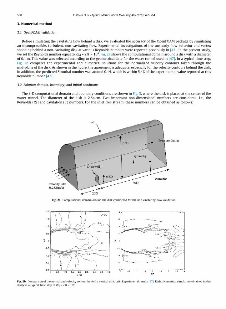
Before simulating the cavitating flow behind a disk, we evaluated the accuracy of the OpenFOAM package by simulatingan incompressible, turbulent, non-cavitating flow. Experimental investigations of the unsteady flow behavior and vortexshedding behind a non-cavitating disk at various Reynolds numbers were reported previously in [47]. In the present study,we set the Reynolds number equal to Red = 2.8 � 104. Fig. 2a shows the computational domain around a disk with a diameterof 0.1 m. This value was selected according to the geometrical data for the water tunnel used in [47]. In a typical time step,Fig. 2b compares the experimental and numerical solutions for the normalized velocity contours taken through themid-plane of the disk. As shown in the figure, the agreement is adequate, especially for the velocity contours behind the disk.In addition, the predicted Strouhal number was around 0.14, which is within 5.4% of the experimental value reported at thisReynolds number [47].
3.2. Solution domain, boundary, and initial conditions
The 3-D computational domain and boundary conditions are shown in Fig. 3, where the disk is placed at the center of thewater tunnel. The diameter of the disk is 2.54 cm. Two important non-dimensional numbers are considered, i.e., theReynolds (Re) and cavitation (r) numbers. For the inlet free stream, these numbers can be obtained as follows:
Fig. 2b.study a
Fig. 2a. Computational domain around the disk considered for the non-cavitating flow validation.
Comparison of the normalized velocity contour behind a vertical disk. Left: Experimental results [47]. Right: Numerical simulation obtained in thist a typical time step of Red = 2.8 � 104.
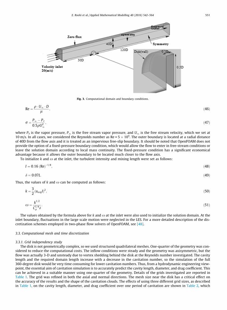
Fig. 3. Computational domain and boundary conditions.
E. Roohi et al. / Applied Mathematical Modelling 40 (2016) 542–564 551
Re ¼ q � U1 � Dl
; ð46Þ
r ¼ P1 � P#0:5qU2
1; ð47Þ
where P0 is the vapor pressure, P1 is the free stream vapor pressure, and U1 is the free stream velocity, which we set at10 m/s. In all cases, we considered the Reynolds number as Re = 5 � 105. The outer boundary is located at a radial distanceof 40D from the flow axis and it is treated as an impervious free-slip boundary. It should be noted that OpenFOAM does notprovide the option of a fixed-pressure boundary condition, which would allow the flow to enter in free-stream conditions orleave the solution domain according to local mass continuity. The fixed-pressure condition has a significant economicaladvantage because it allows the outer boundary to be located much closer to the flow axis.
To initialize k and x at the inlet, the turbulent intensity and mixing length were set as follows:
I ¼ 0:16 ðReÞ�1=8; ð48Þ
d ¼ 0:07L: ð49Þ
Thus, the values of k and x can be computed as follows:
k ¼ 32ðuavgIÞ2; ð50Þ
x ¼ k1=2
C1=4l d
: ð51Þ
The values obtained by the formula above for k and x at the inlet were also used to initialize the solution domain. At theinlet boundary, fluctuations in the large scale motion were neglected in the LES. For a more detailed description of the dis-cretization schemes employed in two-phase flow solvers of OpenFOAM, see [48].
3.3. Computational mesh and time discretization
3.3.1. Grid independency studyThe disk is not geometrically complex, so we used structured quadrilateral meshes. One-quarter of the geometry was con-
sidered to reduce the computational costs. The inflow conditions were steady and the geometry was axisymmetric, but theflow was actually 3-D and unsteady due to vortex shedding behind the disk at the Reynolds number investigated. The cavitylength and the required domain length increase with a decrease in the cavitation number, so the simulation of the full360-degree disk would be very time consuming for lower cavitation numbers. Thus, from a hydrodynamic engineering view-point, the essential aim of cavitation simulation is to accurately predict the cavity length, diameter, and drag coefficient. Thiscan be achieved in a suitable manner using one-quarter of the geometry. Details of the grids investigated are reported inTable 1. The grid was refined in both the axial and normal directions. The mesh size near the disk has a critical effect onthe accuracy of the results and the shape of the cavitation clouds. The effects of using three different grid sizes, as describedin Table 1, on the cavity length, diameter, and drag coefficient over one period of cavitation are shown in Table 2, which
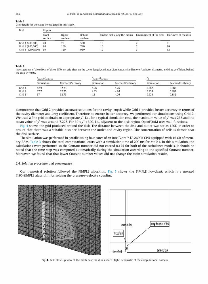
Table 1Grid details for the cases investigated in this study.
Grid Region
Frontsurface
Uppersurface
Behindsurface
On the disk along the radius Environment of the disk Thickness of the disk
Grid 1 (400,000) 70 70 500 10 2 8Grid 2 (900,000) 90 100 740 10 2 10Grid 3 (1,500,000) 90 120 930 10 3 12
Table 2Investigations of the effects of three different grid sizes on the cavity length/cavitator diameter, cavity diameter/cavitator diameter, and drag coefficient behindthe disk, r = 0.05.
Lcavity/dcavitator Dcavity/dcavitator CD
Simulation Reichardt’s theory Simulation Reichardt’s theory Simulation Reichardt’s theory
Grid 1 42.9 32.73 4.26 4.26 0.882 0.882Grid 2 37.7 32.73 4.33 4.26 0.938 0.882Grid 3 37 32.73 4.3 4.26 0.924 0.882
552 E. Roohi et al. / Applied Mathematical Modelling 40 (2016) 542–564
demonstrate that Grid 2 provided accurate solutions for the cavity length while Grid 1 provided better accuracy in terms ofthe cavity diameter and drag coefficient. Therefore, to ensure better accuracy, we performed our simulations using Grid 2.We used a fine grid to obtain an appropriate y+, i.e., for a typical simulation case, the maximum value of y+ was 236 and themean value of y+ was around 7.225. For 30 < y+ < 300, i.e., adjacent to the disk region, OpenFOAM uses wall functions.
Fig. 4 shows the grid produced around the disk. The distance between the disk and outlet was set as 120D in order toensure that there was a suitable distance between the outlet and cavity region. The concentration of cells is denser nearthe disk surface.
The simulation was performed in parallel using four cores of an Intel�Core™ i7-2600K CPU equipped with 16 GB of mem-
ory RAM. Table 3 shows the total computational costs with a simulation time of 200 ms for r = 0.1. In this simulation, thecalculations were performed so the Courant number did not exceed 0.175 for both of the turbulence models. It should benoted that the time step was computed automatically during the simulation according to the specified Courant number.Moreover, we found that that lower Courant number values did not change the main simulation results.
3.4. Solution procedure and convergence
Our numerical solution followed the PIMPLE algorithm. Fig. 5 shows the PIMPLE flowchart, which is a mergedPISO-SIMPLE algorithm for solving the pressure–velocity coupling.
Fig. 4. Left: close-up view of the mesh near the disk surface. Right: schematic of the computational domain.
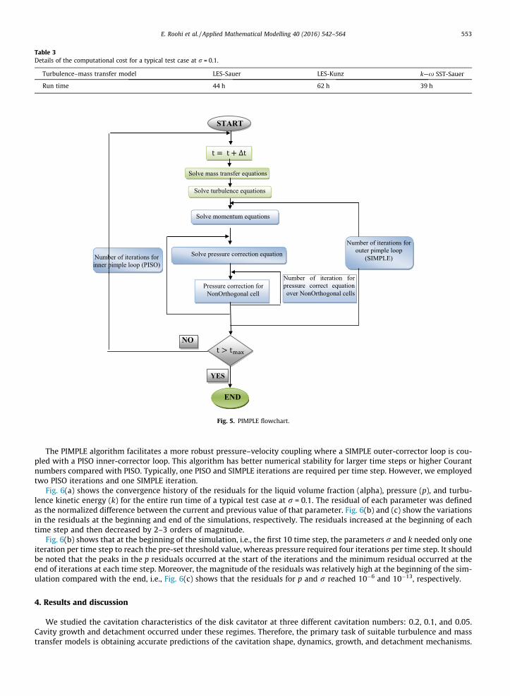
Table 3Details of the computational cost for a typical test case at r = 0.1.
Turbulence–mass transfer model LES-Sauer LES-Kunz k—x SST-Sauer
Run time 44 h 62 h 39 h
START
Solve mass transfer equations
END
Number of iterations for inner pimple loop (PISO)
Solve momentum equations
Number of iteration for pressure correct equation over NonOrthogonal cells
Solve turbulence equations
Pressure correction for NonOrthogonal cell
Number of iterations for outer pimple loop
(SIMPLE)Solve pressure correction equation
NO
YES
Fig. 5. PIMPLE flowchart.
E. Roohi et al. / Applied Mathematical Modelling 40 (2016) 542–564 553
The PIMPLE algorithm facilitates a more robust pressure–velocity coupling where a SIMPLE outer-corrector loop is cou-pled with a PISO inner-corrector loop. This algorithm has better numerical stability for larger time steps or higher Courantnumbers compared with PISO. Typically, one PISO and SIMPLE iterations are required per time step. However, we employedtwo PISO iterations and one SIMPLE iteration.
Fig. 6(a) shows the convergence history of the residuals for the liquid volume fraction (alpha), pressure (p), and turbu-lence kinetic energy (k) for the entire run time of a typical test case at r = 0.1. The residual of each parameter was definedas the normalized difference between the current and previous value of that parameter. Fig. 6(b) and (c) show the variationsin the residuals at the beginning and end of the simulations, respectively. The residuals increased at the beginning of eachtime step and then decreased by 2–3 orders of magnitude.
Fig. 6(b) shows that at the beginning of the simulation, i.e., the first 10 time step, the parameters r and k needed only oneiteration per time step to reach the pre-set threshold value, whereas pressure required four iterations per time step. It shouldbe noted that the peaks in the p residuals occurred at the start of the iterations and the minimum residual occurred at theend of iterations at each time step. Moreover, the magnitude of the residuals was relatively high at the beginning of the sim-ulation compared with the end, i.e., Fig. 6(c) shows that the residuals for p and r reached 10�6 and 10�13, respectively.
4. Results and discussion
We studied the cavitation characteristics of the disk cavitator at three different cavitation numbers: 0.2, 0.1, and 0.05.Cavity growth and detachment occurred under these regimes. Therefore, the primary task of suitable turbulence and masstransfer models is obtaining accurate predictions of the cavitation shape, dynamics, growth, and detachment mechanisms.
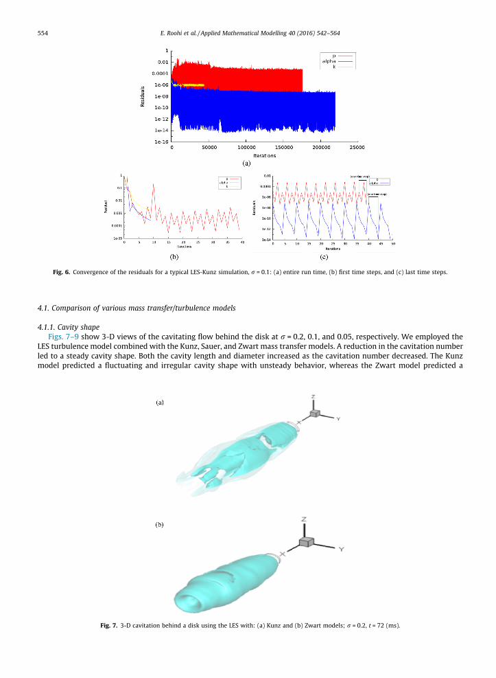
Fig. 6. Convergence of the residuals for a typical LES-Kunz simulation, r = 0.1: (a) entire run time, (b) first time steps, and (c) last time steps.
554 E. Roohi et al. / Applied Mathematical Modelling 40 (2016) 542–564
4.1. Comparison of various mass transfer/turbulence models
4.1.1. Cavity shapeFigs. 7–9 show 3-D views of the cavitating flow behind the disk at r = 0.2, 0.1, and 0.05, respectively. We employed the
LES turbulence model combined with the Kunz, Sauer, and Zwart mass transfer models. A reduction in the cavitation numberled to a steady cavity shape. Both the cavity length and diameter increased as the cavitation number decreased. The Kunzmodel predicted a fluctuating and irregular cavity shape with unsteady behavior, whereas the Zwart model predicted a
Fig. 7. 3-D cavitation behind a disk using the LES with: (a) Kunz and (b) Zwart models; r = 0.2, t = 72 (ms).
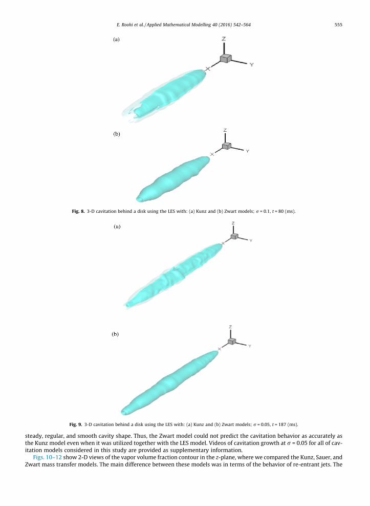
Fig. 8. 3-D cavitation behind a disk using the LES with: (a) Kunz and (b) Zwart models; r = 0.1, t = 80 (ms).
Fig. 9. 3-D cavitation behind a disk using the LES with: (a) Kunz and (b) Zwart models; r = 0.05, t = 187 (ms).
E. Roohi et al. / Applied Mathematical Modelling 40 (2016) 542–564 555
steady, regular, and smooth cavity shape. Thus, the Zwart model could not predict the cavitation behavior as accurately asthe Kunz model even when it was utilized together with the LES model. Videos of cavitation growth at r = 0.05 for all of cav-itation models considered in this study are provided as supplementary information.
Figs. 10–12 show 2-D views of the vapor volume fraction contour in the z-plane, where we compared the Kunz, Sauer, andZwart mass transfer models. The main difference between these models was in terms of the behavior of re-entrant jets. The
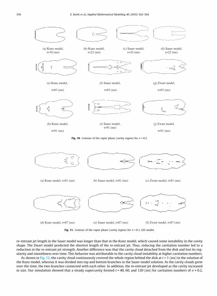
(a) Kunz model, t=10 (ms)
(b) Kunz model, t=22 (ms)
(c) Sauer model, t=10 (ms)
(d) Sauer model, t=22 (ms)
(e) Kunz model,
t=83 (ms)
(f) Sauer model,
t=83 (ms)
(g) Zwart model,
t=83 (ms)
(h) Kunz model,
t=91 (ms)
(i) Sauer model, t=91 (ms)
(j) Zwart model,
t=91 (ms)
Fig. 10. Contour of the vapor phase (cavity region) for r = 0.2.
(a) Kunz model, t=81 (ms) )sm(18=t,ledomtrawZ)c()sm(18=t,ledomreuaS)b(
(d) Kunz model, t=87 (ms) (e) Sauer model, t=87 (ms) (f) Zwart model, t=87 (ms)
Fig. 11. Contour of the vapor phase (cavity region) for r = 0.1, LES model.
556 E. Roohi et al. / Applied Mathematical Modelling 40 (2016) 542–564
re-entrant jet length in the Sauer model was longer than that in the Kunz model, which caused some instability in the cavityshape. The Zwart model predicted the shortest length of the re-entrant jet. Thus, reducing the cavitation number led to areduction in the re-entrant jet strength. Another difference was that the cavity cloud detached from the disk and lost its reg-ularity and smoothness over time. This behavior was attributable to the cavity cloud instability at higher cavitation numbers.
As shown in Fig. 12, the cavity cloud continuously covered the whole region behind the disk at t = 1 (ms) in the solution ofthe Kunz model, whereas it was divided into top and bottom branches in the Sauer model solution. As the cavity clouds grewover the time, the two branches connected with each other. In addition, the re-entrant jet developed as the cavity increasedin size. Our simulation showed that a steady supercavity formed t = 40, 60, and 120 (ms) for cavitation numbers of r = 0.2,
(a) Kunz model, t=1 (ms) (b) Sauer model, t=1 (ms) (c) Zwart model, t=1 (ms)
(d) Kunz model, t=112 (ms) (e) Sauer model, t=112 (ms) (f) Zwart model, t=139 (ms)
(g) Kunz model, t=196 (ms) (h) Sauer model, t=196 (ms) (i) Zwart model, t=187 (ms)
Fig. 12. Contour of vapor phase (cavity region) for r = 0.05, LES model.
E. Roohi et al. / Applied Mathematical Modelling 40 (2016) 542–564 557
0.1, and 0.05, respectively. Two behaviors were observed as the steady supercavity formed: (a) inward movement of thereentrant jet and (b) separation of the subtle vapor bubbles into the main flow due to re-entrant jet movement.
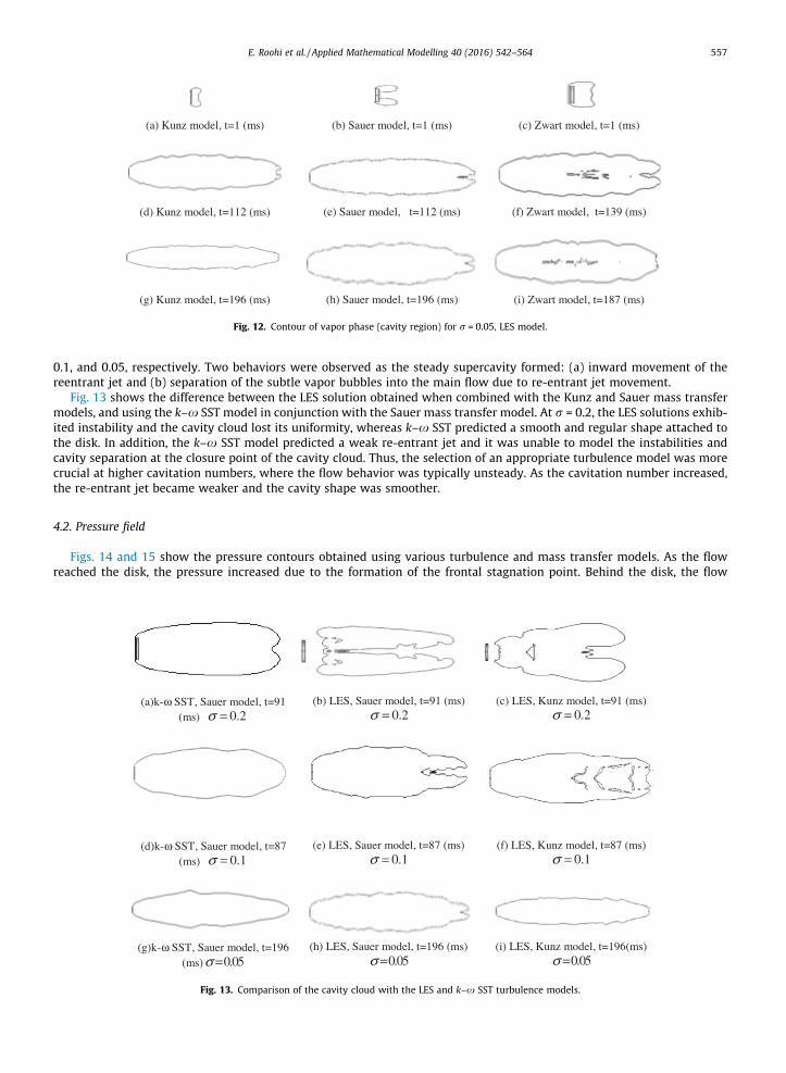
Fig. 13 shows the difference between the LES solution obtained when combined with the Kunz and Sauer mass transfermodels, and using the k–x SST model in conjunction with the Sauer mass transfer model. At r = 0.2, the LES solutions exhib-ited instability and the cavity cloud lost its uniformity, whereas k–x SST predicted a smooth and regular shape attached tothe disk. In addition, the k–x SST model predicted a weak re-entrant jet and it was unable to model the instabilities andcavity separation at the closure point of the cavity cloud. Thus, the selection of an appropriate turbulence model was morecrucial at higher cavitation numbers, where the flow behavior was typically unsteady. As the cavitation number increased,the re-entrant jet became weaker and the cavity shape was smoother.
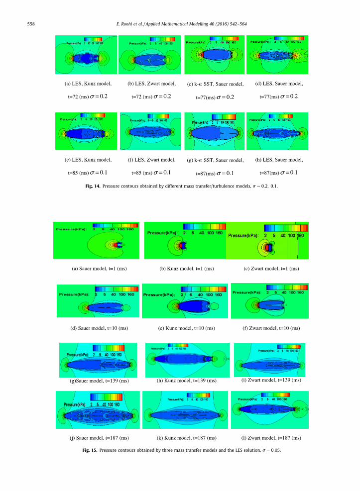
4.2. Pressure field
Figs. 14 and 15 show the pressure contours obtained using various turbulence and mass transfer models. As the flowreached the disk, the pressure increased due to the formation of the frontal stagnation point. Behind the disk, the flow
(a)k-ω SST, Sauer model, t=91 (ms) 0.2σ =
(b) LES, Sauer model, t=91 (ms)0.2σ =
(c) LES, Kunz model, t=91 (ms)0.2σ =
(d)k-ω SST, Sauer model, t=87 (ms) 0.1σ =
(e) LES, Sauer model, t=87 (ms)0.1σ =
(f) LES, Kunz model, t=87 (ms)0.1σ =
(g)k-ω SST, Sauer model, t=196 (ms) 0.05σ =
(h) LES, Sauer model, t=196 (ms)0.05σ =
(i) LES, Kunz model, t=196(ms)0.05σ =
Fig. 13. Comparison of the cavity cloud with the LES and k–x SST turbulence models.
(a) LES, Kunz model,
t=72 (ms) 0.2σ =
(b) LES, Zwart model,
t=72 (ms) 0.2σ =
(c) k-ω SST, Sauer model,
t=77(ms) 0.2σ =
(d) LES, Sauer model,
t=77(ms) 0.2σ =
(e) LES, Kunz model,
t=85 (ms) 0.1σ =
(f) LES, Zwart model,
t=85 (ms) 0.1σ =
(g) k-ω SST, Sauer model,
t=87(ms) 0.1σ =
(h) LES, Sauer model,
t=87(ms) 0.1σ =
Fig. 14. Pressure contours obtained by different mass transfer/turbulence models, r ¼ 0:2; 0:1.
(a) Sauer model, t=1 (ms) (b) Kunz model, t=1 (ms) (c) Zwart model, t=1 (ms)
(d) Sauer model, t=10 (ms) (e) Kunz model, t=10 (ms) (f) Zwart model, t=10 (ms)
(g)Sauer model, t=139 (ms) (h) Kunz model, t=139 (ms) (i) Zwart model, t=139 (ms)
(j) Sauer model, t=187 (ms) (k) Kunz model, t=187 (ms) (l) Zwart model, t=187 (ms)
Fig. 15. Pressure contours obtained by three mass transfer models and the LES solution, r ¼ 0:05.
558 E. Roohi et al. / Applied Mathematical Modelling 40 (2016) 542–564
E. Roohi et al. / Applied Mathematical Modelling 40 (2016) 542–564 559
separated at the sharp edges and the resulting drop in pressure created a vaporous cavity area. A pressure gradient was cre-ated at the interface between the vapor phase and liquid phase, which was due to the pressure difference between the twophases and it was normal to the interface. In addition, cavity shedding and the condensation of cavity bubbles cause ahigh-pressure difference at the closure point of the cavity region. A sharp interface was visible around the cavity domain,which was attributable to the application of the VOF model. The pressure levels were similar with the Sauer and Zwartmodels.
Fig. 14 shows that the Zwart model predicted a lower pressure at the closure point of the cavity cloud compared with theKunz model. This behavior was a result of the lower rate of vapor condensation in this model. Moreover, the region with aconstant vapor pressure expanded to a greater extent in the solution of the Zwart model compared with the Kunz modelsolution, whereas the pressure distribution was almost non-uniform in the Sauer/LES model solutions.
Fig. 15 shows the pressure contours obtained by various mass transfer models at three time steps. At the starting point ofcavity formation, the solutions of the Kunz and Zwart models were similar whereas the Sauer model predicted a dissimilarpressure contour because of the formation of two cavity cloud pieces (Fig. 12(b)). At t = 10 ms, the pressure contours of theZwart model had a stronger re-entrant jet compared with the other models and the cavity length was shorter in this model.At t = 187 ms, the Sauer model exhibited more instability inside the cavity and the Zwart model had the smoothest pressurecontour. A high-pressure region was observed at the closure point of the cavity, which was stronger than that in the Zwartmodel solution.
4.3. Cavity characteristics
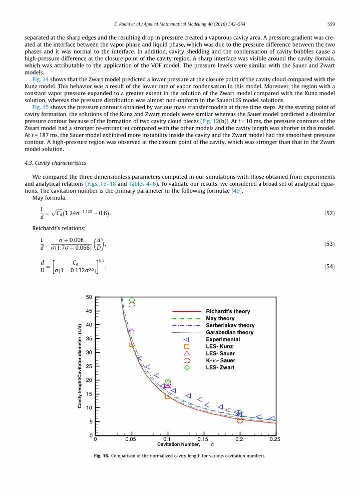
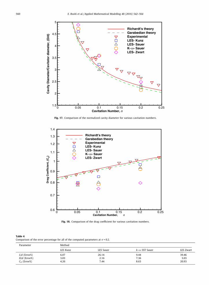
We compared the three dimensionless parameters computed in our simulations with those obtained from experimentsand analytical relations (Figs. 16–18 and Tables 4–6). To validate our results, we considered a broad set of analytical equa-tions. The cavitation number is the primary parameter in the following formulae [49].
May formula:
Ld¼
ffiffiffiffiffiffiCd
p1:24r�1:123 � 0:6� �
: ð52Þ
Reichardt’s relations:
Ld¼ rþ 0:008
rð1:7rþ 0:066ÞdD
� �; ð53Þ
dD¼ Cd
rð1� 0:132r0:5Þ
0:5
; ð54Þ
Cavitation Number, σ
Cav
ity
len
gh
t/C
avit
ato
r d
iam
eter
, (L
/d)
0 0.05 0.1 0.15 0.2 0.250
5
10
15
20
25
30
35
40
45
50
Richardt’s theoryMay theorySerberiakav theoryGarabedian theoryExperimentalLES- KunzLES- SauerK- ω- SauerLES- Zwart
Fig. 16. Comparison of the normalized cavity length for various cavitation numbers.
Cavitation Number, σ
Cav
ity
Dia
met
er/C
avit
ato
r d
iam
eter
, (D
/d)
0 0.05 0.1 0.15 0.2 0.251.5
2
2.5
3
3.5
4
4.5
5
Richardt’s theoryGarabedian theoryExperimentalLES- KunzLES- SauerK- ω- SauerLES- Zwart
Fig. 17. Comparison of the normalized cavity diameter for various cavitation numbers.
Cavitation Number, σ
Dra
g C
oef
fici
ent,
(C
D)
0 0.05 0.1 0.15 0.2 0.250.6
0.7
0.8
0.9
1
1.1
1.2
1.3
1.4
Richardt’s theoryGarabedian theoryExperimentalLES- KunzLES- SauerK- ω- SauerLES- Zwart
Fig. 18. Comparison of the drag coefficient for various cavitation numbers.
Table 4Comparison of the error percentage for all of the computed parameters at r = 0.2.
Parameter Method
LES Kunz LES Sauer k–x SST Sauer LES Zwart
L/d (Error%) 6.07 26.14 9.44 39.46D/d (Error%) 3.03 2.16 7.36 3.03CD (Error%) 4.26 7.44 8.63 20.93
560 E. Roohi et al. / Applied Mathematical Modelling 40 (2016) 542–564
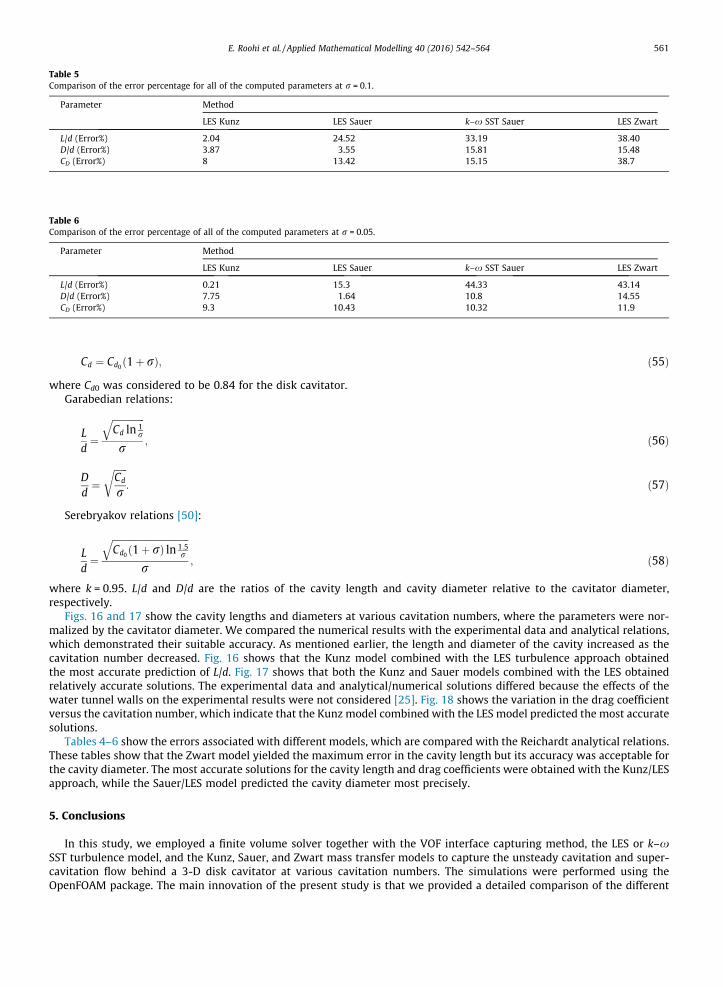
Table 5Comparison of the error percentage for all of the computed parameters at r = 0.1.
Parameter Method
LES Kunz LES Sauer k–x SST Sauer LES Zwart
L/d (Error%) 2.04 24.52 33.19 38.40D/d (Error%) 3.87 3.55 15.81 15.48CD (Error%) 8 13.42 15.15 38.7
Table 6Comparison of the error percentage of all of the computed parameters at r = 0.05.
Parameter Method
LES Kunz LES Sauer k–x SST Sauer LES Zwart
L/d (Error%) 0.21 15.3 44.33 43.14D/d (Error%) 7.75 1.64 10.8 14.55CD (Error%) 9.3 10.43 10.32 11.9
E. Roohi et al. / Applied Mathematical Modelling 40 (2016) 542–564 561
Cd ¼ Cd0ð1þ rÞ; ð55Þ
where Cd0 was considered to be 0.84 for the disk cavitator.Garabedian relations:
Ld¼
ffiffiffiffiffiffiffiffiffiffiffiffiffiffiCd ln 1
r
qr
; ð56Þ
Dd¼
ffiffiffiffiffiffiCd
r
r: ð57Þ
Serebryakov relations [50]:
Ld¼
ffiffiffiffiffiffiffiffiffiffiffiffiffiffiffiffiffiffiffiffiffiffiffiffiffiffiffiffiffiffiffiffiffiCd0 ð1þ rÞ ln 1:5
r
qr
; ð58Þ
where k = 0.95. L/d and D/d are the ratios of the cavity length and cavity diameter relative to the cavitator diameter,respectively.
Figs. 16 and 17 show the cavity lengths and diameters at various cavitation numbers, where the parameters were nor-malized by the cavitator diameter. We compared the numerical results with the experimental data and analytical relations,which demonstrated their suitable accuracy. As mentioned earlier, the length and diameter of the cavity increased as thecavitation number decreased. Fig. 16 shows that the Kunz model combined with the LES turbulence approach obtainedthe most accurate prediction of L/d. Fig. 17 shows that both the Kunz and Sauer models combined with the LES obtainedrelatively accurate solutions. The experimental data and analytical/numerical solutions differed because the effects of thewater tunnel walls on the experimental results were not considered [25]. Fig. 18 shows the variation in the drag coefficientversus the cavitation number, which indicate that the Kunz model combined with the LES model predicted the most accuratesolutions.
Tables 4–6 show the errors associated with different models, which are compared with the Reichardt analytical relations.These tables show that the Zwart model yielded the maximum error in the cavity length but its accuracy was acceptable forthe cavity diameter. The most accurate solutions for the cavity length and drag coefficients were obtained with the Kunz/LESapproach, while the Sauer/LES model predicted the cavity diameter most precisely.
5. Conclusions
In this study, we employed a finite volume solver together with the VOF interface capturing method, the LES or k–xSST turbulence model, and the Kunz, Sauer, and Zwart mass transfer models to capture the unsteady cavitation and super-cavitation flow behind a 3-D disk cavitator at various cavitation numbers. The simulations were performed using theOpenFOAM package. The main innovation of the present study is that we provided a detailed comparison of the different
562 E. Roohi et al. / Applied Mathematical Modelling 40 (2016) 542–564
sets of turbulence and mass transfer models. In addition, the Zwart mass transfer model was added to the OpenFOAMframework. We studied the unsteady growth of the cavity while considering the pressure behavior. We validated ournumerical results using experimental data and analytical relations for the cavity length, diameter, and drag coefficient,which demonstrated their suitable accuracy. We found that the most accurate solutions for the cavity length and dragcoefficient were obtained by applying the LES turbulence model together with the Kunz mass transfer model. TheSauer model combined with the LES turbulence model obtained the most accurate predictions of the cavity diameterresults.
Acknowledgements
The authors acknowledge financial support from the Ferdowsi University of Mashhad under grant No. 30000. The authorsalso acknowledge Dr Eugene de Villiers from ENGYS, UK, and Dr Santiago Marquez Damian, from CIMEC-CONICET, Argentinafor very helpful discussions about turbulence modeling in OpenFOAM. We also acknowledge Mr. Omid Ejtehadi, PhDResearcher at Gyeongsang National University (GNU), and Dr. Craig White, from Glasgow University, UK, for reading andimproving the language of the paper. We also acknowledge the anonymous reviewers of this paper for very helpful sugges-tions, which improved the quality of the manuscript.
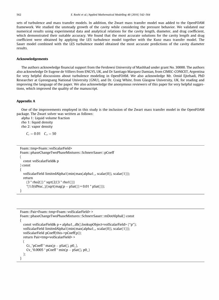
Appendix A
One of the improvements employed in this study is the inclusion of the Zwart mass transfer model in the OpenFOAMpackage. The Zwart solver was written as follows:
alpha 1: Liquid volume fractionrho 1: liquid densityrho 2: vapor density
Cc ¼ 0:01 Cv ¼ 50
Foam::tmp<Foam::volScalarField>Foam::phaseChangeTwoPhaseMixtures::SchnerrSauer::pCoeff(
const volScalarField& p) const{
volScalarField limitedAlpha1(min(max(alpha1_, scalar(0)), scalar(1)));return
(3 * rho2()) * sqrt(2/(3 * rho1()))*(1.0/dNuc_)/(sqrt(mag(p � pSat()) + 0.01 * pSat()));
}
Foam::Pair<Foam::tmp<Foam::volScalarField> >Foam::phaseChangeTwoPhaseMixtures::SchnerrSauer::mDotAlphal() const{
const volScalarField& p = alpha1_.db().lookupObject<volScalarField> (‘‘p’’);volScalarField limitedAlpha1(min(max(alpha1_, scalar(0)), scalar(1)));volScalarField pCoeff(this->pCoeff(p));return Pair<tmp<volScalarField> >(
Cc_⁄pCoeff ⁄max(p � pSat(), p0_),Cv_⁄0.0005 ⁄ pCoeff ⁄min(p � pSat(), p0_)
);}
E. Roohi et al. / Applied Mathematical Modelling 40 (2016) 542–564 563
Appendix A. Supplementary data
Supplementary data associated with this article can be found, in the online version, at http://dx.doi.org/10.1016/j.apm.2015.06.002.
References
[1] C.E. Brennen, Cavitation and Bubble Dynamics, Oxford University Press, Oxford, UK, 1995.[2] M. Self, J.F. Ripken, Steady state cavity studies in free-jet water tunnel, St. Anthony Falls Hydrodynamic Laboratory Report No. 47, 1955.[3] G. Wang, S.M. Ostoja, Large eddy simulation of a sheet/cloud cavitation on a NACA0015 hydrofoil, Appl. Math. Model. 31 (2007) 417–447.[4] R.F. Kunz, D.A. Boger, D.R. Stinebring, T.S. Chyczewski, J.W. Lindau, H.J. Gibeling, A preconditioned Navier–Stokes method for two-phase flows with
application to cavitation, Comput. Fluids 29 (2000) 849–875.[5] N.H. Singhal, A.K. Athavale, M. Li, Y. Jiang, Mathematical basis and validation of the full cavitation model, J. Fluids Eng. 124 (2002) 1–8.[6] C.L. Merkle, J. Feng, P.E.O. Buelow, Computational modelling of the dynamics of sheet cavitation, in: Proceedings of the Third International Symposium
on Cavitation, (CAV1998), Grenoble, France, 1998.[7] J. Sauer, Instationaren kaviterende Stromung – Ein neues Modell, baserend auf Front Capturing (VoF) and Blasendynamik (PhD thesis), Universitat
Karlsruhe, 2000.[8] W. Yuan, J. Sauer, G.H. Schnerr, Modelling and computation of unsteady cavitation flows in injection nozzles, J. Mech. Ind. Eng. 2 (2001) 383–394.[9] P. Zwart, A.G. Gerber, T. Belamri, A two-phase model for predicting cavitation dynamics, in: ICMF 2004 International Conference on Multiphase Flow,
Yokohama, Japan, 2004.[10] I. Senocak, W. Shyy, Evaluation of cavitation models for Navier–Stokes computations, in: Proceeding of FEDSM 02, ASME Fluid Engineering Division
Summer Meeting, Montreal, Canada, 2002.[11] Y. Chen, C.J. Lu, L.P. Xue, Validation of HEM-based cavitation for cavitation flows around disk, in: New Trends in Fluid Mechanics Research, Proceedings
of the 5th International Conference on Fluid Mechanics, Shanghai, China, 2007.[12] M. Passandideh-Fard, E. Roohi, Coalescence collision of two droplets: bubble entrapment and the effects of important parameters, in: Proceeding of the
14th Annual (International) Mechanical Engineering Conference, Isfahan, Iran, 2006.[13] Z. Shang, Numerical investigations of supercavitation around blunt bodies of submarine shape, Appl. Math. Model. 37 (20) (2013) 8836–8845.[14] M. Passandideh-Fard, E. Roohi, Transient simulations of cavitating flows using a modified volume-of-fluid (VOF) technique, Int. J. Comput. Fluid Dyn.
22 (2008) 97–114.[15] M. Frobenius, R. Schilling, R. Bachert, B. Stoffel, G. Ludwig, Three-dimensional unsteady cavitating effects on a single hydrofoil and in a radial pump-
measurement and numerical simulation, in: Proceedings of the 5th International Symposium on Cavitation, Cav03-GS-9-005, Osaka, 2003.[16] S. Wiesche, Numerical simulation of cavitation effects behind obstacles and in an automotive fuel jet pump, Heat Mass Transfer 41 (2005) 615–624.[17] A. Bouziad, M. Farhat, F. Gunning, K. Miyagawa, Physical modelling and simulation of leading edge cavitation, application to an industrial inducer, in:
Proceedings of the 5th International Symposium on Cavitation, Cav03-OS-6-014, Osaka, Japan, 2003.[18] D. Li, M. Grekula, P. Lindell, A modified k–x SST turbulence model to predict the steady and unsteady sheet cavitation on 2D and 3D hydrofoils, in:
Proceedings of the 7th International Symposium on Cavitation, CAV2009, 2009.[19] T. Huuva, Large Eddy Simulation of Cavitating and Non-cavitating Flow (PhD thesis), Chalmers University of Technology, Sweden, 2008.[20] D. Liu, S. Liu, Y. Wu, H. Xu, LES numerical simulation of cavitation bubble shedding on ALE 25 and ALE 15 hydrofoils, J. Hydrodyn. 21 (6) (2009) 807–
813.[21] N.X. Lu, R.E. Bensow, G. Bark, LES of unsteady cavitation on the delft twisted foil, J. Hydrodyn., Ser. B 22 (5) (2010) 784–791.[22] R.F. Kunz, T. Chyczewski, D. Boger, D. Stinebring, H. Gibeling, T.R. Govindan, Multi-phase CFD analysis of natural and ventilated cavitation about
submerged bodies, in: Proceedings of FEDSM 99, 3rd ASME/JSME Joint Fluids Engineering Conference, 1999.[23] N.M. Nouri, M. Moghimi, S.M.H. Mirsaeedi, Numerical simulation of unsteady cavitating flow over a disk, Proc. Inst. Mech. Eng., Part C: J. Mech. Eng. Sci.
224 (2010) 1245–1253.[24] M. Baradaran Fard, A.H. Nikseresht, Numerical simulation of unsteady 3D cavitating flows over axisymmetric cavitators, Sci. Iran. Trans. B: Mech. Eng.
19 (2012) 1258–1264.[25] J. Guo, C. Lu, Y. Chen, Characteristics of flow field around an underwater projectile with natural and ventilated cavitation, J. Shanghai Jiaotong
University (Science) 16 (2) (2011) 236–241.[26] Z. Shang, D.R. Emerson, G.U. Xiaojun, Numerical investigations of cavitation around a high speed submarine using OpenFOAM with LES, Int. J. Comput.
Methods 9 (2012) 1250040–1250054.[27] E. Roohi, A.P. Zahiri, M. Passandideh-Fard, Numerical simulation of cavitation around a two-dimensional hydrofoil using VOF method and LES
turbulence model, Appl. Math. Model. 37 (2013) 6469–6488.[28] M. Morgut, E. Nobile, Numerical predictions of cavitating flow around model scale propellers by CFD and advanced model calibration, J. Rotating Mach.
2012 (2012) 618180.[29] B. Ji, X.W. Luo, R.E.A. Arndt, X.X. Peng, Y.L. Wu, Large eddy simulation and theoretical investigations of the transient cavitating vortical flow structure
around a NACA66 hydrofoil, Int. J. Multiph. Flow 68 (2015) 121–134.[30] B. Ji, X.W. Luo, R.E.A. Arndt, Y.L. Wu, Numerical simulation of three dimensional cavitation shedding dynamics with special emphasis on cavitation
vortex interaction, Ocean Eng. 87 (2014) 64–77.[31] B. Ji, X.W. Luo, Y.L. Wu, X.X. Peng, Y.L. Duan, Numerical analysis of unsteady cavitating turbulent flow and shedding horse-shoe vortex structure around
a twisted hydrofoil, Int. J. Multiph. Flow 51 (2015) 33–43.[32] OpenFOAM, <http://www.openfoam.com>.[33] G.H. Schnerr, J. Sauer, Physical and numerical modeling of unsteady cavitation dynamics, in: Proceedings of 4th International Conference on
Multiphase Flow, New Orleans, USA, 2001.[34] F.R. Menter, Two-equation eddy-viscosity turbulence models for engineering applications, AIAA J. 32 (8) (1994) 1598–1605.[35] F. Menter, J. Carregal Ferreira, T. Esch, B. Konno, The SST turbulence model with improved wall treatment for heat transfer predictions in gas turbines,
in: Proceedings of the International Gas Turbine Congress, Tokyo, Japan, IGTC2003-TS-059, 2003, pp. 2–7.[36] R.E. Bensow, G. Bark, Simulating cavitating flows with LES in OpenFOAM, in: J.C.F. Pereira, A. Sequeira (Eds.), Lisbon European Conference on
Computational Fluid Dynamics, ECCOMAS CFD, Portugal, 2010.[37] N.X. Lu, Large Eddy Simulation of Cavitating Flow on Hydrofoil (Licentiate of Engineering thesis), Department of Shipping and Marine Technology,
Chalmers University of Technology, Göteborg, Sweden, 2010.[38] P. Sagaut, Large Eddy Simulation for Incompressible Flows, third ed., Springer, New York, 2006.[39] C. Fureby, F. Grinstein, Large eddy simulation of high-Reynolds number free and wall-bounded flows, J. Comput. Phys. 181 (2002) 68–97.[40] S. Ghosal, An analysis of numerical errors in large-eddy simulations of turbulence, J. Comput. Phys. 125 (1996) 187–206.[41] E. De Villiers, The Potential of Large Eddy Simulation for the Modelling of Wall Bounded Flows (PhD thesis), Department of Mechanical Engineering,
Imperial College, London, UK, 2006.[42] A.G. Kravchenko, P. Moin, R. Moser, Zonal embedded grids for numerical simulations of wall-bounded turbulent flows, J. Comput. Phys. 127 (1996)
412–423.

564 E. Roohi et al. / Applied Mathematical Modelling 40 (2016) 542–564
[43] R.E. Bensow, C. Fureby, On the justification and extension of mixed methods in LES, J. Turbul. 8 (2007) N54.[44] S.M. Damiána, M.N. Nigro, Comparison of single phase laminar and large eddy simulation (LES) solvers using the OpenFOAM suite, in: Eduardo
Dvorkin, Marcela Goldschmit, Mario Storti (Eds.), Computacional, vol. XXIX, Buenos Aires, Argentina, 2010, pp. 3721–3740.[45] F.H. Hirt, B.D. Nichols, Volume of fluid (VOF) method for the dynamics of free boundaries, J. Comput. Phys. 39 (1981) 201–225.[46] H.G. Weller, A new approach to VOF-based interface capturing methods for incompressible and compressible flow, Technical Report, OpenCFD Ltd,
2008.[47] J.J. Miau, T.S. Leu, T.W. Liu, J.H. Chou, On vortex shedding behind a circular disk, Exp. Fluids 23 (1997) 225–233.[48] J. Klostermann, K. Schaake, R. Schwarze, Numerical simulation of a single rising bubble by VOF with surface compression, Int. J. Numer. Meth. Fluids 71
(8) (2013) 960–982.[49] A. May, Water entry and the cavity-running behavior of missiles, Final Technical Report NAVSEA Hydroballistics Advisory Committee, Silver Spring,
MD, 1975.[50] V. Serebryakov, Supercavitation flows with gas injection prediction and drag redaction problems, in: Fifth International Symposium on Cavitation
(CAV2003), Osaka, Japan, CAV 03-OS-7-003, 2003.


![home [profdoc.um.ac.ir]profdoc.um.ac.ir/articles/a/1030669.pdf · home For Authors Editorial Board current issue All Issues Next issue contact Research for Quality Management:: Asian](https://img.pdfslide.us/doc/110x75/5e0ff97724e9b57ee72fd105/home-home-for-authors-editorial-board-current-issue-all-issues-next-issue-contact.jpg)