applied mathematical methods for partial differential ...eaton.math.rpi.edu/CSUMS/Papers/Waves/Chapter3.pdfapplied mathematical methods for partial differential equations Isom H. Herron

applied mathematical methods forpartial differential equations

Isom H. Herron & Michael R. Foster

Department of Mathematical Sciences

Rensselaer Polytechnic Institute

Troy, NY 12180-3590

January 16, 2007

Chapter 3

Eigenvalue Problems

OUTLINE

3.1. Preamble3.2. Synge�s setup for Rayleigh�s criterion3.2.1 Exercises

3.3. Sturm-Liouville problems3.3.1 Exercises3.3.2 Prüfer�s method3.3.3 Orthogonality of eigenfunctions3.3.4 Expansions in eigenfunctions

3.4 Worked Examples3.4.1 Heat conduction in a non-uniform rod3.4.2 Waves on shallow water3.4.3 Exercises

3.5. Synge�s proof of Rayleigh�s criterion3.5.1 Exercises

3.6. Non-standard eigenvalue problems3.6.1 L� = �M�

3.6.2 Exercises3.6.3 Sturm-Liouville problems with weight changing sign (counter-rotating

cylinders)3.6.4 Singular Sturm-Liouville problems3.6.5 Orthogonality of Bessel Functions3.6.6 Continuous Spectra3.6.7 Exercises

1

2 CHAPTER 3 EIGENVALUE PROBLEMS

3.1 Preamble

In the twentieth century there were a number of innovations in applied math-ematical technique. Some had their origins in the years before. Rayleighseems to have begun many of these innovations taken up by others in thelast century. There is a criterion, due to Rayleigh, for establishing instabilityof a rotating �uid. Based on elementary physical arguments, he was ableto conclude (loosely) that the �ow con�guration is stable when the squareof the circulation increases outwards. In the early years of the last centurywork was done to put many of these physical arguments on a stronger math-ematical footing. One of the techniques which has proven to be useful is thestudy of eigenvalue problems for di¤erential equations. These relate particu-larly to the method of normal modes of vibration of a physical system. Thegeneral mathematical ideas were �rst developed by Sturm and Liouville, butFourier had laid much of the groundwork in his theory of heat conduction.This �continuous�treatment, by means of di¤erential equations, has discreteanalogs as well, in the theories of matrices and of particle systems.

3.2 Synge�s setup for Rayleigh�s Criterion

In his study of the stability of a rotating heterogeneous liquid J. L. Syngeused the following approach [15]. Cylindrical coordinates (r; �; z) are em-ployed to analyze the rotating motion of an inviscid �uid about the z�axis,with velocity having components (u; v; w); the momentum equations may bereduced to

@u

@t+ u

@u

@r+ w

@u

@z� v2

r= �1

�

@p

@r; (3.1)

@

@t(rv) + u

@

@r(rv) + w

@

@z(rv) = 0; (Circumferential)

@w

@t+ u

@w

@r+ w

@w

@z= �1

�

@p

@z: (Axial)

Though the density may not be constant, the �uid is assumed to beincompressible so that

@�

@t+ u

@�

@r+ w

@�

@z= 0: (3.2)

3.2 SYNGE�S SETUP FOR RAYLEIGH�S CRITERION 3

The mass-conservation equation then reduces to

@

@r(ru) +

@

@z(rw) = 0; (3.3)

so that the velocity �eld is solenoidal. When the density � is assumed to bea function of r only, a solution to the equations of motion may thus be foundwhere

u = 0; v = v(r); w = 0; � = �(r); p = p(r): (3.4)

The only stipulation on the equations of motion is a balance between thecentrifugal force and the pressure gradient:

v2

r=1

�

dp

dr: (3.5)

Small perturbations are imposed on the motion (3.4) of the form

(u; v; w) = (u0; v + v0; w0); � = ��+ �0; p = p+ p0: (3.6)

These are substituted into the equations of motion (3.1)-(3.3) and the non-linear terms neglected:

@u0

@t� 2vv

0

r= �1

�

@p0

@r+�0

�2dp

dr; (3.7)

@

@t(rv0) + u0

d

dr(rv) = 0;

@w0

@t= �1

�

@p0

@z;

@�0

@t+ u0

d�

dr= 0:

It is then possible to eliminate p0; �0; and v0; and using the centrifugal balance(3.5) obtain a single partial di¤erential equation for u0 and w0 :

�@3u0

@z@t2� @

@r

��@2w0

@t2

�+ F (r)

@u0

@z= 0;

where

F (r) =1

r3d

dr(�r2v2): (3.8)


However, since the velocity �eld is axisymmetric there exists a stream func-tion such that

ru0 = �@ @z; rw0 =

@

@r;

and continuity (3.3) is identically satis�ed. Thus a single equation results for

@

@r

��

r

@3

@r@t2

�+�

r

@4

@z2@t2+F

r

@2

@z2= 0: (3.9)

A normal mode solution is sought for traveling waves of the from

= �(r)eik(z�ct); (3.10)

where k is a wave number, c is the wave speed. The wave number is takento be real, thereby localizing the disturbance. The wave speed is allowed tobe complex. The �ow is said to be temporally stable if all disturbances ofthe form (3.10) decay in time, i.e. ci < 0: Likewise, the �ow is said to betemporally unstable, if there is a disturbance of the form (3.10) which growsin time, i.e. ci > 0:The resulting ordinary di¤erential equation for � is found by substituting

(3.10) into (3.9) to be

d

dr

��

r

d�

dr

�+

�c�2

F

r� k2

�

r

�� = 0: (3.11)

Typical boundary conditions for a wall-bounded �ow at r = r1 and r = r2are @ =@z = 0 for r = r1 and r = r2 and therefore

� (r1) = � (r2) = 0: (3.12)

This is an example of an eigenvalue problem in which a solution � is obtainedfor certain values c�2 when the wave number and the coe¢ cients are giventhrough the basic �ow.

Example 1 : Suppose that the �uid has the density distribution �� = �0r; �0constant, and performs solid body rotation such that �v = !0r; !0 constant.Then from (3.8), the function

F (r) =1

r3d

dr

��0!

20r5�= 5�0!

20r: (3.13)

The resulting form of the equation for � is, from (3.11)

�00+ (5!20c

�2 � k2)� = 0: (3.14)

3.3 STURM-LIOUVILLE PROBLEMS 5

3.2.1 Exercises

Exercise 1 Determine the function F (r) (3.8) for the case of solid bodyrotation when � = �0, constant. What is the resulting form of the equationfor �?

3.3 Sturm-Liouville Problems

The standard form for a Sturm-Liouville problem is a second order di¤erentialequation of the form

d

dx

�P (x)

dy

dx

�+ (�R(x)�Q(x)) y = 0; (3.15)

de�ned on a �nite interval a < x < b; with separated boundary conditions

�0y(a) + �1y0 (a) = 0; (3.16)

�0y (b) + �1y0 (b) = 0:

The real constants �0; �1; �0; and �1 are assumed to be �xed, but no twocorresponding to one end-point are both zero. There are well developedtheories of the existence of solutions to the equation. For our purposes,we need only have that P (x), R(x) and Q(x) are continuous real-valuedfunctions and P (x) > 0 on a � x � b: The di¤erential equation and theboundary conditions together de�ne a regular Sturm-Liouville problem. Itshould be noted that there is no loss of generality in the factored form of thedi¤erential equation. An equation in the form

P2(x)d2y

dx2+ P1 (x)

dy

dx+ P0(x)y = 0;

may be put in factored form by multiplying through the equation by theintegrating factor

�(x) =1

P2(x)eR P1(x)P2(x)

dx

There are properties of the solutions of the Sturm-Liouville problem(3.15)-(3.16) that are easy to obtain. Others require a deeper analysis. Wewill derive the properties as needed for the solution of the stability problem.


Property (i) : If throughout the interval (a; b); R(x) is of one sign, thenall of the eigenvalues � are real.

Property (i ): If throughout the interval (a; b); Q(x) � 0; and �0�1 � 0;and �0�1 � 0; then all eigenvalues are real. Note: P (x) > 0; but R(x)may change sign on (a; b):

Property (ii): If throughout the interval (a; b); R(x) is of one sign,Q(x) > 0; �0�1 � 0; and �0�1 � 0; then all the eigenvalues � have thesign of R(x):

Property (ii ): If all the conditions of Property (ii) hold except that R(x)changes sign in (a; b); then there are both positive and negative eigen-values �:

To demonstrate Property (i), suppose that � is complex. Then write

� = �1 + i�2;

in terms of its real and imaginary parts. As would be the case for the eigenvec-tor of a problem involving matrices, we must suppose that the eigenfunctiony(x) is also complex. Write

y(x) = y1(x) + iy2(x);

in terms of the real and imaginary parts. Multiply the Sturm-Liouville equa-tion (3.15) by y(x) = y1(x)� iy2(x) and integrate from x = a to x = b: Afterintegration by parts, the result is

[P (x)y0(x)y(x)]x=bx=a�

Z b

a

P (x) jy0(x)j2 dx+Z b

a

(�R(x)�Q(x)) jy(x)j2 dx = 0;(3.17)

where jy(x)j2 = (y1(x))2 + (y2(x))2 ; with a similar meaning for the modulusof the derivative y0(x): Since the boundary conditions are real, �y(x) satis�esthem as does y(x): Thus, evaluating the boundary contributions

[P (x)y0(x)y(x)]ba = �P (b)

�0�1jy(b)j2 + P (a)

�0�1jy(a)j2 ;

when neither �1 = 0 nor �1 = 0: If either of these constants is 0; the boundarycontribution at the corresponding endpoint is clearly seen to be 0; since y(x)vanishes at that endpoint.


The important observation now is that the boundary contributions arereal. Taking the imaginary part of (3.17) gives

�2

Z b

a

R(x) jy(x)j2 dx = 0: (3.18)

Since R(x) does not change sign on (a; b); �2 = 0:Property (ii) is established by considering the real part of (3.17). It

follows that

�1

Z b

a

R(x) jy(x)j2 dx =Z b

a

P (x) jy0(x)j2 dx+Z b

a

Q(x) jy(x)j2 dx+

+P (b)�0�1jy(b)j2 � P (a)

�0�1jy(a)j2 : (3.19)

By the same reasoning as for the imaginary part (3.18), and the demonstra-tion of Property (i), the boundary contributions are nonnegative under theassumptions P (x) > 0; �0�1 � 0; and �0�1 � 0: Given P (x) > 0; Q(x) > 0;then �1 > 0 if R(x) > 0 on (a; b) or �1 < 0; if R(x) < 0 on (a; b); since theintegral term multiplying �1 in (3.19) has the sign of R(x):Property (ii) gives su¢ cient conditions for no eigenvalue to be negative,

when R(x) > 0; while Property (ii ) gives su¢ cient conditions for both posi-tive and negative eigenvalues, if R(x) changes sign. However, if Q(x) changessign on (a; b) (which violates Property (ii)), while R(x) has one sign, it ispossible for there to be only a �nite number of negative eigenvalues. Prop-erty (ii ) however, allows as it turns out, an in�nite number of eigenvalues ofboth signs, This will be shown most easily after the introduction of Prüfer�smethod to follow.

Example 2 : For the case of solid body rotation, where � = �0r (Example1), we can assert, on the basis of Property (i), that all eigenvalues c�2 arereal, since P (r) = 1; R(r) = 5!20 > 0; and since Q(r) = k2 > 0; theeigenvalues will be positive for conditions like (3.12), where in the notationof (3.16), �1 = �1 = 0:

3.3.1 Exercises

Exercise 2 Prove Property (i ).


Exercise 3 Show, on the basis of Property (i) that the eigenvalues c�2 ofExercise 1 are all real.

Exercise 4 The following Sturm-Liouville problem occurs in the energystability theory of �ow between rotating cylinders [9]:

(r�0(r))0+�

r�(r) = 0; 0 < a < r < b;

� = 0; at r = a; b:

Show that the eigenfunctions are

�n = sin[p�n ln(r=b)];

with eigenvalues

�n =n2�2

[ln(a=b)]2; n = 1; 2; � � �

Exercise 5 Analyze the Sturm-Liouville problem

y00+ (�+ 2 sech 2x)y = 0; �a < x < a;

y(�a) = y(a) = 0:

Method: If � = �k2; show that one solution of the di¤erential equation isekx(tanh x�k); and �nd another by replacing k by �k; show that the two areusually linearly independent and investigate the exceptional cases. Find thegeneral solution if � = +�2: Then apply the boundary conditions and describequalitatively the nature of the eigenvalues and eigenfunctions.

Exercise 6 Consider the Sturm-Liouville problem

y00+

�� 2

(1 + x)2

�y = 0; 0 < x < 1;

y(0) = y(1) = 0:

(a) Show that the eigenvalues are all positive, based on Property (ii).(b) If � = k2; the general solution is

y = c1

�cos kx

1 + x+ k sin kx

�+ c2

�sin kx

1 + x� k cos kx

�:

Apply the boundary conditions, and derive a transcendental equation to de-termine the eigenvalues. Find an accurate approximation to the smallesteigenvalue. Describe qualitatively the nature of the eigenfunctions. For asolution see section 3.4.


Exercise 7 (a) Show that the di¤erential equation

x4y00 + �y = 0; a < x < b;

may be solved exactly in terms of Bessel functions, and �nally in the elemen-tary form

y = x

�c1 cos

�k

x

�+ c2 sin

�k

x

��; k =

p�:

(b) Apply the boundary conditions y(a) = y(b) = 0; and show that theeigenvalues are

�n = n2�2�ab

L

�2;

where L = b� a; with eigenfunctions

yn(x) = x sin

�n�b

L

�1� a

x

��:

Exercise 8 Consider the boundary value problem

y00 + �xy = 0; �1 < x < 1;

y(�1) = y(1) = 0:

(a) On the basis of Property (i), conclude that all of the eigenvalues are real.(b) Show implicitly, that if � is an eigenvalue, so is ��:(c) The equation may be solved explicitly in terms of Airy functions (). Showthat the general solution may be written as y = c1Ai(kx) + c2Bi(kx); for asuitable k: Find the eigenvalue relation, and show that it also gives the sameresult as part (b). Indicate the locations of the eigenvalues. By use of Maple,or some computer algebra system, determine the locations of the �rst feweigenvalues of smaller magnitudes.


y00 + � sgn(x)y = 0; �1 < x < �; (3.20)

y(�1) = y(�) = 0;

where sgn(x) =

8<: 1; if x > 0

�1; if x < 0: The coe¢ cient R(x) = sgn(x) is discon-

tinuous, but continuously di¤erentiable solutions may be found by requiring


y(0+) = y(0�); and y0(0+) = y0(0�): With this proviso, show that (3.20)has all real eigenvalues, but an in�nite number of both positive and negativeeigenvalues. Find an explicit formula for the corresponding eigenfunctions.Obtain a numerical approximation to the eigenvalue of smallest magnitude.

Unusual phenomena may happen if the boundary conditions are not sep-arated. It is then possible that there may be more than one eigenfunctioncorresponding to an eigenvalue, but clearly not more, since the equation isof second order. This, and other possibilities are illustrated in the followingexercises.


y00 + �y = 0; �� < x < �;

with periodic boundary conditions

y(��) = y(�);

y0(��) = y0(�):

Show that the eigenvalues are �n = n2; n = 0; 1; : : : ; with eigenfunctionsy0 = 1; yn = fcos(nx); sin(nx)g:Exercise 11 Consider the boundary value problem

y00 + �y = 0; 0 < x < 1;

with

y(0)� y(1) = 0;

y0(0) + y0(1) = 0:

Show that every value of � is an eigenvalue and determine a correspondingeigenfunction.

Exercise 12 Show that the boundary value problem

y00 + �y = 0; 0 < x < 1;

2y(0) + y(1) = 0; 2y0(0) + y0(1) = 0;

has no real eigenvalues. Determine its (complex) eigenvalues and its eigen-functions.


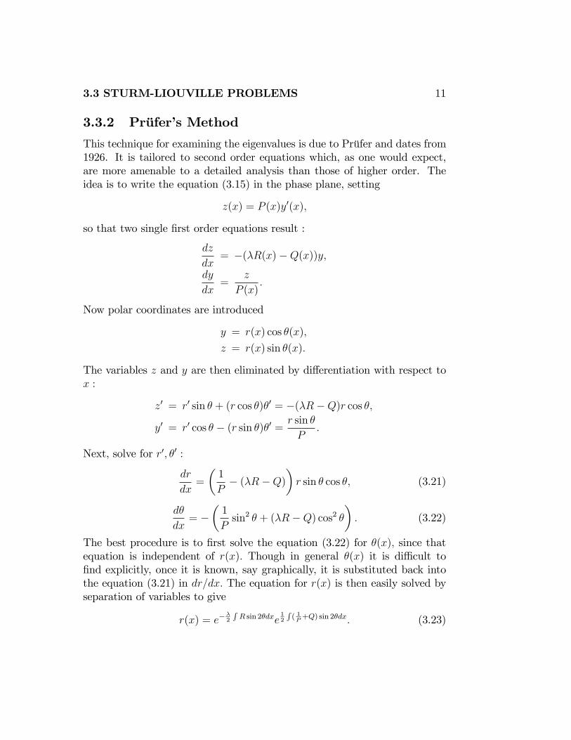
3.3.2 Prüfer�s Method

This technique for examining the eigenvalues is due to Prüfer and dates from1926. It is tailored to second order equations which, as one would expect,are more amenable to a detailed analysis than those of higher order. Theidea is to write the equation (3.15) in the phase plane, setting

z(x) = P (x)y0(x);

so that two single �rst order equations result :

dz

dx= �(�R(x)�Q(x))y;

dy

dx=

z

P (x):

Now polar coordinates are introduced

y = r(x) cos �(x);

z = r(x) sin �(x):

The variables z and y are then eliminated by di¤erentiation with respect tox :

z0 = r0 sin � + (r cos �)�0 = �(�R�Q)r cos �;

y0 = r0 cos � � (r sin �)�0 = r sin �

P:

Next, solve for r0; �0 :

dr

dx=

�1

P� (�R�Q)

�r sin � cos �; (3.21)

d�

dx= �

�1

Psin2 � + (�R�Q) cos2 �

�: (3.22)

The best procedure is to �rst solve the equation (3.22) for �(x); since thatequation is independent of r(x): Though in general �(x) it is di¢ cult to�nd explicitly, once it is known, say graphically, it is substituted back intothe equation (3.21) in dr=dx: The equation for r(x) is then easily solved byseparation of variables to give

r(x) = e��2

RR sin 2�dxe

12

R( 1P+Q) sin 2�dx: (3.23)


Remark 1 : There is a periodicity associated with the function �(x): Thatis, if �(x) is a solution, so is �(x) + n�; for every integer n: This followsmost easily from the de�nition of y(x). Since y(x) = r cos �(x);

r cos[�(x) + n�] = r cos �(x) cos(n�) = (�1)nr cos �(x) = (�1)ny(x)

andr sin[�(x) + n�] = r sin �(x) cos(n�) = (�1)nPy0(x):

For even values of n, the same solution is obtained,while for odd values of n;the negative of the solution is obtained, which is also a solution. A solutiony(x) of (3.15) has a zero at x = x1; if and only if, �(x1) = �

2+n�: The zeros

are simple, that is if y(x1) = 0; then y0(x1) 6= 0: This latter condition followsfrom the fact that cos �(x1) and sin �(x1) will not both vanish.

Remark 2 : Notice from the equation (3.22) in d�=dx; for R(x) > 0; �(x;�)is a decreasing function of �; and if �(xn;�) = (n� 1

2)�; for integer n; then

�(x;�) < (n� 12)� for x > xn: This follows since

d�(xn;�)

dx=

�1P (xn)

< 0:

Boundary Conditions. The previous boundary conditions (3.16) are used.Since

tan � =z

y=Py0

y;

take �(a;�) = ; where is the smallest possible number, ��2� < �

2; such

that tan = ��0P (a)=�1 (If �1 = 0; take = ��2); that is

�(a;�) = tan�1�P (a)y0(a)

y(a)

�= :

Similarly, take ��2< � � �

2so that tan � = ��0P (b)=�1: (If �1 = 0; then

take � = �2:) Then the boundary conditions on � are therefore

�(a) = ; (3.24a)

�(b) = �: (3.24b)

The boundary conditions are only important for �(x). Once � is determinedr(x) follows from (3.23).


Remark 3 : A solution y(x) of (3.15) is an eigenfunction of the Sturm-Liouville problem (3.15-3.16) if

�(a;�) = ; (3.24c)

�(b;�) = � � n�; n = 0; 1; 2; : : : : (3.24d)

Suppose �(x;�) satis�es �(a;�) = : Owing to the fact that � (b;�) is adecreasing function of �, it is possible to show, using the conditions of Remark2, that �(b;�) is unbounded as � ! �1: Thus, it must be that � ! �1:On the other hand, it turns out that as � increases from �1; there is a �rstvalue � for which the second of the boundary conditions (3.24d) is satis�ed.For this eigenvalue, �(b;�0) = �: As � increases, there is an in�nite sequence�n for which the second boundary condition is satis�ed, namely those forwhich �(b;�) = � � n�; by Remark 1. For each of these

yn(x) = rn(x) cos �(x;�n):

Furthermore, the eigenfunction belonging to �n has exactly n zeros in theinterval a < x < b: This follows from counting the zeros of yn(x) as describedin Remark 1.It is now possible to establish Property (ii ), using some of the previous

results. The formulation (3.15)-(3.16) remains the same. Remark 1 is stillvalid. However, Remark 2 is not, since R(x) changes sign. It is true though,that on a subinterval [a0; b0] on which R(x) > R0 > 0; P (x) < P0; andQ(x) < Q0; �(x;�) is a decreasing function of �; and �(x;�) ! �1; as� ! 1: This is readily established by comparing �(x;�) with the solution!0(x;�) satisfying an equation like (3.22) with constant coe¢ cients P0; Q0;and R0 :

d!0dx

= � 1

P0sin2 !0 � (�R0 �Q0) cos

2 !0:

The successive zeros of !0(x;�) have spacing �[P0=(�R0�Q0)]12 ; which tends

to zero as � ! 1: Hence !0 ! �1 as � ! 1: A standard comparisonargument [4] gives that �(x;�) ! �1 as � ! 1: Likewise, on an interval[a1; b1] on which R(x) < R1 < 0; P (x) < P1; and Q(x) < Q1; a comparisonis made with the solution !1(x;�) satisfying an equation like (3.22) withconstant coe¢ cients P1; Q1; and R1 :

d!1dx

= � 1

P1sin2 !1 � (�R1 �Q1) cos

2 !1:


In this case �(x;�) ! �1 as � ! �1: Thus, in any case, �(b;�) ! �1as � ! �1: This shows that there are an in�nite number of positive andnegative eigenvalues.

3.3.3 Orthogonality of Eigenfunctions

The simple Sturm-Liouville problem

y00 + �y = 0; 0 < x < �;

y(0) = 0; y(�) = 0;

has eigenfunctions yn = sinnx, where n = 1; 2; ::: These form the basis ofthe Fourier sine series. The construction of the series is based on the notionthat the functions sinnx are orthogonal on the interval [0; �] :Z �

0

sinnx sinmxdx = 0; m 6= n:

A similar relation holds for the eigenfunctions of a regular Sturm-Liouvilleproblem, with one important generalization, the introduction of a weightfunction.

Property (iii): When the conditions of Property (i) hold, then the eigen-functions of the regular Sturm-Liouville system (3.15), (3.16) havingdi¤erent eigenvalues are orthogonal with weight function R(x): Thatis, given eigenvalues �n; �m (�n 6= �m) and corresponding eigenfunc-tions yn; ym Z b

a

R(x)yn(x)ym(x)dx = 0; m 6= n: (3.25)

Property (iv): When the conditions of Property (i) hold, where withoutloss of generality it is assumed that R(x) > 0; then the eigenfunctionsof the regular Sturm-Liouville system (3.15-3.16 ) may be normalizedwith weight function R(x); so thatZ b

a

R(x)y2n(x)dx = 1:


Property (iv ): When the conditions of Property (ii) hold, and if theeigenfunctions corresponding to positive and negative eigenvalues aredenoted by y+n and y�n respectively, then the eigenfunctions may benormalized as Z b

a

R(x)�y+n�2dx = 1;

and Z b

a

R(x)�y�n�2dx = �1:

3.3.4 Expansions in Eigenfunctions

A very important question about a sequence of eigenfunctions yn of a Sturm-Liouville problem, orthogonal and square integrable with respect to a weightfunction R(x); is the following: Can every square-integrable function f beexpanded into an in�nite series f =

Pcnyn of the yn? With a suitable

meaning attached to sense of convergence of the series, the answer to thisquestion is a¢ rmative, and the sequence of eigenfunctions yn is said to becomplete.The expansion coe¢ cients for an expansion in the eigenfunctions of the

typical problem (3.15)-(3.16) are found by assuming for a suitable functionf(x)

f =X

cnyn: (3.26)

Then by (3.25)Z b

a

f(x)R(x)ym(x)dx =X

cn

Z b

a

R(x)yn(x)ym(x)dx

= cm

Z b

a

R(x)y2m(x)dx:

The detailed proof of the convergence of (3.26) will not be presented (See[1]). However, what makes the proof particularly a¤ecting is that it dependson the asymptotic behavior of the eigenfunctions of the Sturm-Liouville prob-lem. Suppose that the equation is written in �Liouville Normal Form�

u00(t) + (�� q(t))u(t) = 0; (3.27)


which is obtained by setting

y(x) =u(t)

4pP (x)R(x)

; t =

R xa

pR(x)=P (x)dxR b

a

pR(x)=P (x)dx

(3.28)

in (3.15). Thus, for large n; it may be shown that if in (3.16), �1�1 6= 0; then

un(t) vp2 cos(n�t) + O

�1

n

�as n!1: (3.29)

If the condition �1�1 = 0 holds in (3.16), then cos(n�t) is replaced by sin(n�t)in (3.29).

The nonhomogeneous problem

Consider the inhomogeneous boundary value problem

d

dx

�P (x)

dy

dx

�+(�R(x)�Q(x)) y := Ly+�Ry = f(x); a < x < b (3.30)

B1y = �0y(a) + �1y0 (a) = 0; (3.31)

B2y = �0y (b) + �1y0 (b) = 0:

Here � is a given �xed constant and f is known. The boundary conditions arethe same as (3.16) but � may or may not be an eigenvalue of (3.15)-(3.16).We examine conditions for (3.30)-(3.31) to have a solution.Multiply (3.30) by some eigenfunction '(x) of (3.15)-(3.16) and integrate

from x = a to x = b to obtainZ b

a

(Ly + �Ry)'dx =

Z b

a

f'dx:

Employing integration by parts and the boundary conditions (3.31) the leftside becomes Z b

a

y(L'+ �R')dx

and using the fact that ' is an eigenfunction with eigenvalue � the result isZ b

a

y(��R'+ �R')dx =

Z b

a

f'dx:

3.4 WORKED EXAMPLES 17

Thus if � is the eigenvalue �, a solution for y depends on whether or notR baf'dx = 0:Suppose that (3.30)-(3.31) has a solution. Using the eigenfunction ex-

pansions based on (3.15)-(3.16), set

f =1Xn=1

An'n(x); y =1Xn=1

Bn'n(x):

Since f is known, so are the coe¢ cients An; however the values Bn have tobe determined. Substituting into (3.30) leads to

1Xn=1

Bn(��n + �)R'n(x) =

1Xn=1

An'n(x):

This reinforces the previous result. If � 6= �n for all n; a solution may befound since the eigenfunctions are orthogonal with weight R(x): The coe¢ -cients are given by

Bn =AnR ba('n(x))

2 dx

(�� n)R ba('n(x))

2R(x)dx; n = 1; 2; : : :

However, if � = �n0 for some n0; the problem has no solution unless An0 = 0for that n0: In this case, the solution is given by

y =1Xn=1

Bn'n(x);

where the coe¢ cient Bn0 is arbitrary. In e¤ect, there are �in�nitely many�solutions.

3.4 Worked Examples

3.4.1 Heat conduction in a non-uniform rod

Consider heat conduction governed by the parabolic di¤erential equation

�c@u

@t=

@

@x

��(x)

@u

@x

�; 0 < x < L; t > 0 (3.32)


u(0; t) = u(L; t) = 0:

Here �(x) is the density, c(x) the speci�c heat and �(x) the conductivity [11,Sec. 4.1]. Solving by separation of variables let u(x; t) = '(x)e��t in (3.32)to �nd

(�(x)'0)0+ ��c' = 0;

'(0) = '(L) = 0:

To be speci�c, we study the model problem where L = 1 and

�(x) =1

(1 + x)2= �(x)c(x):

The resulting Sturm-Liouville problem looks like�'0

(1 + x)2

�0+

�

(1 + x)2' = 0:

In order to have the equation look like (3.27), use the substitution (3.28) andset

w(x) ='(x)

(1 + x);

giving

w00 +

�� 2

(1 + x)2

�w = 0; (3.33)

w(0) = w(1) = 0: (3.34)

Using MAPLE or some other CAS �nd that the general solution is

w = a

�cos kx

1 + x+ k sin kx

�+ b

�sin kx

1 + x� k cos kx

�; (3.35)

where k =p�: Applying the left boundary condition

w(0) = a� bk = 0: (3.36)

The right boundary condition gives

w(1) = a

�cos k

2+ k sin k

�+ b

�sin k

2� k cos k

�= 0: (3.37)


0 2 4 6 8 10 12-1

-0.8

-0.6

-0.4

-0.2

0

0.2

0.4

0.6

0.8

1

k

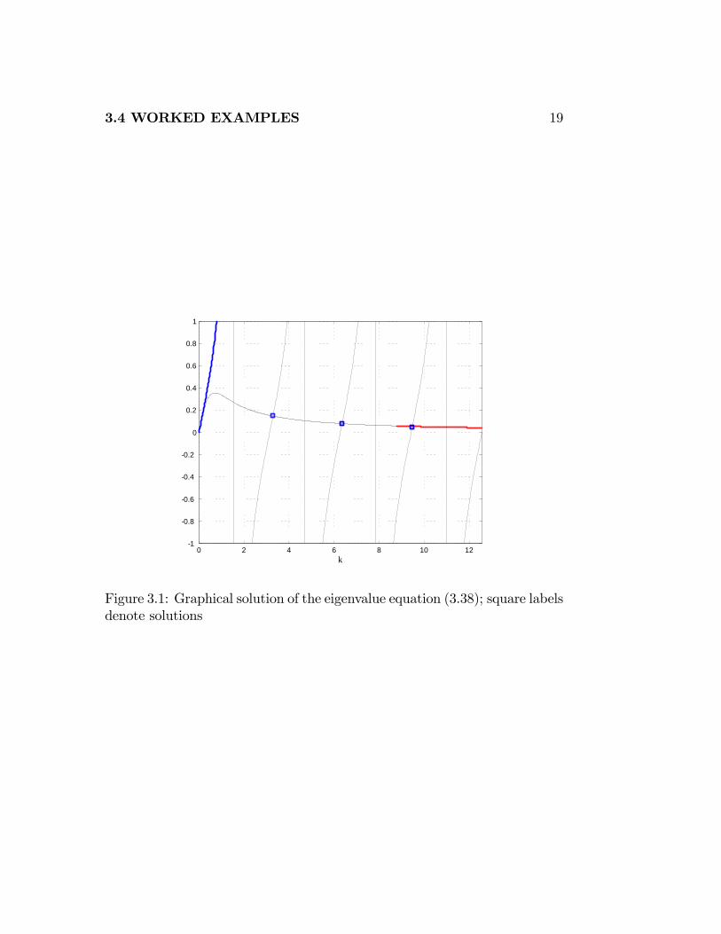
Figure 3.1: Graphical solution of the eigenvalue equation (3.38); square labelsdenote solutions


The simultaneous solution of (3.36) and (3.37) leads to�� 1 �k12cos k + k sin k 1

2sin k � k sin k

�� = 0:The characteristic equation which determines the eigenvalues is therefore

tan k =k

1 + 2k2: (3.38)

As expected from the earlier work, there are an in�nite number of eigenvalues�n = k2n; n = 1; 2 : : : ; determined from the solutions of the transcendentalequation shown graphically.The lowest eigenvalue is �1

:= 10:8: One �nds that � = 0 is not an

eigenvalue since the general solution of (3.33) would be w = a(1+x)�1+b(1+x)2; and satisfying (3.34) gives a = b = 0: We also observe that tan kn � 0as n ! 1: Hence �n � n2�2: Furthermore, from (3.35) and (3.36) we havethat normalized wn(x) �

p2 sin(n�x); all in keeping with the remarks below

(3.29).

3.4.2 Waves on shallow water

A channel of varying width and bottom topography supports water waves.The governing equation is given by

@2u

@t2=g

b

@

@x

�bh@u

@x

�;

for the displacement u(x; t); where b(x) is the breadth and h(x) is depthof the channel, and g is the acceleration due to gravity [3, Sec. 2.1]. Weexamine the special case where the channel is measured from x = 0 to x =1; h (x) = (1 + x)2; b(x) = 1 + x: By separation of variables we obtain theform

u(x; t) = y(x)ei!t;

which gives an equation for the spatial mode shapes�(1 + x)3y0

�0+ �(1 + x)y = 0; (3.39)


where � = !2=g: We take the channel to be closed at both ends so we havethe boundary conditions

y(0) = y(1) = 0: (3.40)

Together (3.39) and (3.40) form a Sturm-Liouville problem, so we know thatits eigenvalues are real and are non-negative by properties (i) and (ii) ofsection 3.3. Further, the eigenvalue � = 0 is excluded since the generalsolution of (3.39) would be

y = c1 + c2(1 + x)�2;

with which (3.40) would give

c1 + c2 = 0;

c1 +1

4c2 = 0:

For all� (3.39) is an Euler-Cauchy type equation so it has solutions of theform

y = (1 + x)s;

and substituting in we �nd

s(s+ 2) + � = 0:

Solving, obtains = �1�

p1� �:

To satisfy y(0) = 0; set

y = (1 + x)�1+p1�� (1 + x)�1�

p1��:

The condition y(1) = 0 gives

2p1�� = 1:

If � < 1 so thatp1� � is real, this equation clearly has no solution. If

� = 1; the two solutions are no longer linearly independent. In particularfor � = 1; two independent solutions are (1 + x)�1 and (1 + x)�1 ln(1 + x):The condition at x = 0 is satis�ed by the latter, but not it does not vanishat x = 1: Thus � = 1 is not an eigenvalue.


For � > 1; the square root becomes imaginary. We can still obtain twosolutions by the method of setting

(1 + x)�1+ip��1 = (1 + x)�1ei

p��1 ln(1+x)

= (1 + x)�1hcos�p

�� 1 ln(1 + x)�+ i sin

�p�� 1 ln(1 + x)

�i:

Two independent solutions of (3.39) are given by the real and imaginaryparts of this expression; that is, by

(1 + x)�1 cos�p

�� 1 ln(1 + x)�and (1 + x)�1 sin

�p�� 1 ln(1 + x)

�:

To make y(0) = 0 we put

y(x) = (1 + x)�1 sin�p

�� 1 ln(1 + x)�:

The condition y(1) = 0 gives

sin�p

�� 1 ln(2)�= 0:

Thus,p�� 1 ln 2 must be an integral multiple of � :

p�� 1 ln 2 = n�; or

�n =n2�2

(ln 2)2+ 1; n = 1; 2; 3; :::

These then, are the eigenvalues. The corresponding eigenfunctions are

yn(x) = (1 + x)�1 sin

�n�ln(1 + x)

ln 2

�:

We turn next to the expansion problem. By the results on Sturm-Liouvilleproblems ([1]), these eigenfunctions are complete. We have the generalizedFourier series

f(x) s1Xn=1

cnyn(x);

where with the weight function R(x) = (1 + x)�1 from (3.39). Conditionson f(x) that ensure the convergence of the generalized Fourier series andthe series solution to the related initial value problem follow directly [18].For instance, we might want to solve the partial di¤erential equation givenu(x; 0) = f(x); ut(x; 0) = 0:


3.4.3 Exercises

Exercise 13 Consider the problem of expanding a function f(x) de�ned on[��; �] in terms of the eigenfunctions of Exercise 10. Assume that

f(x) =1Xn=0

cnyn:

Show that the desired expansion becomes

f(x) =a02+

1Xn=0

[an cos(nx) + bn sin(nx)] ;

wherea02= c0 =

1

2�

Z �

��f(x)dx;

an =1

�

Z �

��f(x) cos(nx)dx;

bn =1

�

Z �

��f(x) sin(nx)dx:

This is called the full-range Fourier series expansion of f(x):


y00 +2

(x+ 1)y0 + �y = 0; 0 < x < 1; (y)

y0(0) = 0; y(1) = 0:

(a) Put the equation in the standard form (3.15).(b) Show that the substitution u(x) = (1+x)y(x) in (y) leads to the di¤erentialequation

u00 + �u = 0 (0 < x < 1):

What are the corresponding boundary conditions on u?(c) Determine the eigenfunctions un, while �nding a transcendental relationgiving the eigenvalues �n and hence show that

yn = cnsin(

p�n(1� x))

1 + x; n = 1; 2; : : : :

(d) Write down suitable expressions for the coe¢ cients cn so the eigenfunc-tions are normalized.



y00 + 2y0 + (1 + �)y = 0; 0 < x < 1; (yy)

y0(0) = 0; y0(1) = 0

(a) Show that �n = n2�2 is the nth eigenvalue for (yy) ( n = 1; 2; � � � ); andgive a corresponding eigenfunction yn: Is there an eigenvalue �0?(b) Find R(x) such that

(yn; ym) =

Z 1

0

R(x)yn(x)ym(x)dx = 0;

where m 6= n:

(c) Determine cn such that e�x =1Pn=0

cnyn(x):

Exercise 16 (a) Show that the substitution u(x) = exy(x) in (yy) leads tothe di¤erential equation

u00 + �u = 0 (0 < x < 1):

What are the corresponding boundary conditions on u?(b) Normalize the eigenfunctions un as 'n = un= kunk and hence show that

'n sp2 cos(n�x) as n!1:


y00 + �y = 0; 0 < x < 1;

with the boundary conditions

y(0) = 0; y0(1) = ��y(1) � constant:

(a) Show that the eigenfunctions are of the form

yn = sin knx; (3.41)

when � > 0; where kn; n = 1; 2;, are the roots of the equation

tan k = �k�; (3.42)


and the eigenvalues �n = k2n: Consider separately the cases � > 0; � = 0; � <0: Note: If � < 0; there is the possibility of a non-positive eigenvalue, sinceall of the conditions of Property (ii) of Section 3.3 are not met. Determinethe corresponding eigenfunction in this special case and the transcendentalequation for the eigenvalue.(b) Show that the eigenfunctions are orthogonal by making use of (3.42), andnormalize them as 'n = yn= kynk : Hence show that the normalizing constantsdepend on n if � 6= 0:


y00 + �y = 0; 0 < x < 1;

y0(0) = 0; y(1) + y0(1) = 0:

(a) Determine the eigenfunctions and a transcendental equation which givesthe eigenvalues. Find a numerical approximation to �1; the smallest eigen-value, and show that �n v n2�2 as n!1:(b) Show that the eigenfunctions are orthogonal by making use of the charac-teristic equation found in part (a). Normalize them as 'n = yn= kynk ; henceverifying that the normalizing constants depend on n: Show that

'n sp2 cos(n�x) as n!1


y00 � 2y0 + (1 + �)y = 0; 0 < x < 1

y(0) = 0; y(1) + y0(1) = 0:

(a) If �n is the nth eigenvalue for the problem (n = 1; 2; � � � ) ; obtain a tran-scendental equation determining �n and give a corresponding eigenfunctionyn:(b) Find R(x) such that

(yn; ym) =

Z 1

0

R(x)yn(x)ym(x)dx = 0;

where m 6= n:

(c) Determine cn such that ex =1Pn=0

cnyn(x):


Exercise 20 Consider the eigenvalue problem given in Exercise ?? whena < 1 and _b = 1:(a) If f(r) is de�ned on [a; 1] show that

f(r) =

1Xn=1

cn sin

�n� ln r

ln a

�;

where

cn =

R 1af(r) sin

�n� ln rln a

�drrR 1

asin2

�n� ln rln a

�drr

:

Introduce an appropriate change of variables and show that this reduces to

cn = 2

Z 1

0

f(at) sin(n�t)dt:

(b) Evaluate cn when f(r) = 1 and when f(r) = r:

Exercise 21 Suppose the nonhomogeneous problem of interest is

d

dx

�P (x)

dy

dx

�+ (�R(x)�Q(x)) y := Ly + �Ry = 0; a < x < b (3.43)

B1y : = �0y(a) + �1y0 (a) = 1; (3.44)

B2y : = �0y (b) + �1y0 (b) = 2:

Here 1 and 2 are nonzero constants.Derive analogous conditions to those in section 3.3.4.for the existence

of a solution. Consider the alternatives if � is or is not an eigenvalue of(3.15)-(3.16). (i) Argue why if � is an eigenvalue then if 1 2 6= 0; there isa solution only under special conditions. Show this by multiplying (3.43) byan eigenfunction ' of (3.15)-(3.16) and integrating from x = a to b: Notehowever, that the solution is not unique since any eigenfunction may addedto give another solution. Hence there are �in�nitely many� solutions (ii) If� is not an eigenvalue argue why if 1 2 6= 0; there is a unique solution.Hint: Examine the general solution y = c1'1+ c2'1 to (3.43) where the basicsolutions '1 and '2 are chosen so that B1'1 = 0 and B2'2 = 0:This permits the analysis of the more general boundary value problem of

(3.30) and (3.44) by writing the solution by superposition as the sum of eachof the two types.

3.5 SYNGE�S PROOF OF RAYLEIGH�S CRITERION 27

Exercise 22 As an illustration of the results of Exercise 21, consider theproblem of �nding the steady-state temperature distribution T (r) in a longcylindrical annulus a � r � b as the solution to the boundary value problem

d

dr(rdT

dr) = 0;

�0T (a) + �1dT

dr(a) = 1; �0T (b) + �1

dT

dr(b) = 2:

The boundary conditions indicate that the heat exchange is prescribed on thewalls, and that they may not be perfectly insulated.(i) Suppose �1 = �1 = 0: Show that the homogeneous problem has only thetrivial solution. Hence �nd the unique solution to the nonhomogeneous prob-lem.(ii) Suppose �0 = �0 = 0: Show that the homogeneous problem has the so-lution T = T0; constant. This corresponds to an eigenvalue � = 0; as aSturm-Liouville problem. Integrate the di¤erential equation to �nd condi-tions on the �uxes in order that a solution exists.

3.5 Synge�s Proof of Rayleigh�s Criterion

We turn our attention again to (3.11) now recognizable as a typical Sturm-Liouville problem, in the form (3.15). Synge recognized this and made thefollowing observations.

Since��

r> 0; and

k2��

r> 0;

by Property (i ), the eigenvalues c�2 are real. Furthermore, if

F > 0 on (r1; r2);

then by Property (ii), all values of c�2 are positive. Hence c is real andthe oscillation (3.10) is stable. On the other hand, if

F < 0 on (r1; r2);

then, also by Property (ii), c�2 is negative. The value of c with positiveimaginary part give instability. If F changes sign on (r1; r2); then by


Property (ii), c�2 takes both positive and negative values, and hencethere is instability. Thus from (3.8), a necessary and su¢ cient conditionfor stability is

d

dr(��r2�v2) > 0;

which is Rayleigh�s Criterion.

Example 3 The case treated in Examples 1 and 2, where �� = �0r with solidbody rotation (3.14), may be solved explicitly under the boundary conditions(3.12). Since the equation has constant coe¢ cients, the eigenfunctions willbe expressible as

�n = sin[q5!20c

�2n � k2(r � r1)];

and the eigenvalues are found to be

c�2n =1

5!20

�n2�2

(r2 � r1)2+ k2

�; n = 1; 2; : : :

3.5.1 Exercises

Exercise 23 Consider the stability equation (Exercise 1) for solid body ro-tation �v = !0r (!0 const) in a cylinder where 0 � r � b:(a) Solve explicitly and show that the eigenfunctions are expressible in termsof a Bessel function of integer order, and determine the eigenvalues.(b) Find an algebraic expression for the smallest eigenvalue �1 = 1=c2 interms of !0; kand b: Thus verify that the �ow is stable.

3.6 Non-Standard Eigenvalue Problems

The theory of Sturm-Liouville problems has been shown to be useful. Nev-ertheless, there are many other eigenvalue problems that arise, not of thatparticular type. For instance, the order of the equation may be higher thantwo, and the eigenvalue may occur multiplying a di¤erential operator. Thistype of generalized eigenvalue problem was �rst treated systematically byKamke. Some authors therefore refer to these as Kamke Problems. It is tothese types of problems we turn next. Rather than elaborate the completetheory, it will be illustrated by several applied problems.

3.6 NON-STANDARD EIGENVALUE PROBLEMS 29

3.6.1 L�=�M�

Example 4 : The study of Rossby waves in a closed ocean illustrates atype of non-standard eigenvalue problem. A simple example is given by theeigenvalue problem for Rossby normal modes governed by

r2 = ��@ @x

in R;

= 0 on @R;

in a closed rectangular basin de�ned by R = (0; �) � (0; Y ); where is thequasi-geostrophic stream function, (x; y) are the (eastward, northward) coor-dinates and @R is the boundary of R: This is reduced to a one-dimensionalproblem using separation of variables by setting

(x; y) = �(x) sin ky:

Hence, k = m�=Y; m = 1; 2; ::: The resulting ordinary di¤erential equationis

d2�

dx2� k2� = �i�d�

dx;

with boundary conditions � (0) = � (�) = 0: The resulting eigenvalues andeigenfunctions are

�2n = 4(n2 + k2);

�n(x) = e�i�nx=2 sinnx; n = 1; 2; :::

In a notation similar to the heading of this subsection, write L� = �M�where the operators are de�ned as

L =d2

dx2� k2;

M = �i ddx:

This notation for the operatorM; though less common in Fluid Mechanics, isvery prevalent in Quantum Physics. The completeness and expansion theoryfor a class of problems of this type was carried out by Masuda [12]. (See alsoMishoe [14], who did not have the geophysical application in mind.)


Example 5 When the stability of �ow between rotating cylinders is studiedin the viscous regime, the earlier derivation of the stability equations must beextended. This was carried out by G. I. Taylor in 1923. By an ingenious blendof experiment and theory, he was able to conclude that when the cylindersrotate in the same direction, an instability, observed in the form of vortices,could be described quite accurately mathematically. A companion result, onegeneralizing Rayleigh�s Criterion, was later derived by Synge [16], [2]. Heproved stability if

!2r22 > !1r

21;

where !1 and r1 are angular velocity and radius respectively, of the innercylinder, and !2 and r2 are the corresponding quantities for the outer cylin-der. The linearized disturbances he treated were also assumed to be axisym-metric and periodic in the axial direction. The resulting system of ordinarydi¤erential equations is

M�Mu+ T�2�1

r2� �

�v = ��Mu; (3.45a)

u+M0v = ��v; (3.45b)

u = u0 = v = 0; at r = �; 1;

where

Mw =

�� d2

dr2� 1r

d

dr+1

r2+ �2

�w; � < r < 1:

The parameters occurring in the system are the Taylor number T , wave num-ber �; � = r1=r2; � = !2=!1; and 0 < � = (1 � �=�2)=(1 � �) < 1. Theoperators M� and M0 operate in the same way as M; but they all have dif-ferent domains by virtue of the boundary conditions. The important numberis �; which is the temporal growth rate. If Re (�) < 0; the �ow is stable.Synge recognized that by multiplying the �rst equation (3.45a) by r�u; andintegrating from r = � to r = 1; certain positive de�nite integrals result.However, one term remains which involves both u and v: For that reason, thesecond equation (3.45b) must be multiplied by some positive weight functionW (r) and v; and the result integrated. When the two expressions are addedthe result is

hM�Mu; ui+ T�2��

1

r2� �

�v; u

�+ hu;Wvi+ hM0v;Wvi =


= �� (hMu; ui+ hWv; vi) (3.46)

where

hf; gi :=Z 1

�

rf(r)�g(r)dr:

A logical choice for W (r) is �T�2(1=r2 � �) since on � � r � 1;T (1=r2 � �) < 0; for the �ows under consideration. By taking the real partof (3.46), it is possible to determine Re(�): The result is

hMu;Mui+Re (hM0v;Wvi) = �Re(�)(hMu; ui+ hWv; vi): (3.47)

The second term on the left of (3.47) reduces as

Re(hM0v;Wvi) = Re

�Z 1

�

�� d

dr

�rd

dr

�+1

r+ �2r

�vW (r)�vdr

�=

Z 1

�

W (r)

r

��dvdr��2 + jvj2r + �2r jvj2

!dr +Re

�Z 1

�

rdv

dr�vW 0(r)dr

�

=

Z 1

�

rW (r)

��dvdr � v

r

��2 + �2 jvj2!dr > 0:

The last step is determined by the fact that since W 0(r) = 2T�2=r3;

Re

�Z 1

�

rW 0(r)dv

dr�vdr

�=1

2

Z 1

�

W 0(r)rd

drjvj2 dr = �

Z 1

�

W (r)d

drjvj2 dr:

Consequently, from (3.47), Re(�) < 0; and the stability result holds.

The structure of the formulation (3.45a), (3.45b) is seen to be of thegeneral form of a matrix operator equation L� = �M�; where

L =

0@M�M T�2�1r2� ��

1 M0

1A ;

� =

0@ u

v

1A ;

M =

0@M 0

0 1

1A ;


and � = ��: The completeness and expansion theory for this problem was�rst carried out by DiPrima and Habetler [5].

Example 6 Another important problem of hydrodynamic stability that canbe cast in this form occurs in the study of the problem of Rayleigh-Bénard con-vection. In its most basic form, assuming a Boussinesq �uid, the linearizedstability equations for the vertical velocity and temperature perturbations maybe reduced to a system with constant coe¢ cients [9]

(D2 � a2)2w � a2Ra� =�sPr(�D2 + a2)w; (3.48)

(�D2 + a2)� � w = �s�; (3.49)

where D = d=dz: Here Ra is the Rayleigh number and Pr is the Prandtlnumber The boundary conditions are taken to be rigid and conducting at thetop and bottom:

w = Dw = � = 0 at z = 0; 1:

The general formulation makes it clear why the principle of exchange of sta-bilities holds for this problem. That is, if Ra < 0; then Re(s) < 0; so the �owis stable, and if Ra > 0; then Im(s) = 0: To see this simply set w = �1 and�2 = a2Ra�: Then the system becomes0@M�M �1

�1 1a2Ra

M0

1A0@ �1�2

1A = �s

0@ 1PrM 0

0 1a2Ra

1A0@ �1�2

1A :

Since M�M and M0 are both positive de�nite on their domains, if Ra > 0;the operator equation

L� = �sM�;has the property that L = L�; M =M� and hM�;�i > 0 in a suitable innerproduct, so the eigenvalues s are all real. However if Ra < 0; then M isno longer a de�nite operator, though it is symmetric. In that case complexeigenvalues s = �+ i! may occur. However, it is possible to show that � < 0:Form the inner product

hL�;i = �s hM�;i ;

where

=

0@ �1

��2

1A :


Then, sincehL�;i =

R 10

�j(�D2 + a2)�1j2 � �2 ��1 + �1 ��2 � 1

a2R(jD�2j2 + a2j�2j2)

�dz;

and Ra < 0; Re hL�;i > 0: On the other handhM�;i = 1

Pr

R 10

hjD�2j2 + a2j�2j2 � 1

a2Raj�2j2

idz; which is positive.

Consequently Re(s) < 0:

3.6.2 Exercises

Exercise 24 Consider the buckling of a column with constant sti¤ness EI:Suppose that the column is of length L and is cantilevered at its base, that isy0(0) = 0; where y (x) is the de�ected shape. For a uniform column, Eulerbeam theory says that

EIy00 = P [y(l)� y(x)] ; 0 < x < L;

y(0) = 0; y0(0) = 0:

Di¤erentiating to get rid of y(L); obtain the eigenvalue problem

y000 + �y0 = 0; 0 < x < L;

y(0) = y0(0) = y00(L) = 0;

where � = P=EI:Show that all of the eigenvalues are real and positive without solving com-pletely for all the eigenfunctions.Find the eigenvalues and corresponding eigenfunctions or �buckling modes�.In particular, show that the critical (minimum) buckling load is

Pcr =�2EI

4L2:

Sketch the critical buckling mode.

Exercise 25 Solve the system (3.48)-(3.49) with stress-free conducting bound-ary conditions

w = D2w = � = 0; at z = 0; 1:

Show that the system may be reduced to

(D2 � a2)(D2 � a2 � s=Pr)(D2 � a2 � s)w = �a2Raw:


Hence show that the eigenfunctions are wn(z) = sin(n�z); n = 1; 2; : : : witheigenvalues sn = �1

2(1+Pr)(n2�2+a2)�

�14(Pr�1)2(n2�2 + a2)2 + a2Ra Pr =(n

2�2 + a2)�1=2

:Notice that if Ra < 0 complex eigenvalues may indeed occur.

Exercise 26 Find the eigenvalues and eigenfunctions of the boundary valueproblem

y0000 + �y00 = 0; 0 < x < 1;

y(0) = y0(0) = y(1) = y00(1) = 0:

3.6.3 Sturm-Liouville problems with weight changingsign (counter-rotating cylinders)

The consequences of Rayleigh�s Criterion being violated are usually describedsimply as an instability; in�nitesimal disturbances are predicted to grow intime. This is often evidenced by the emergence of a secondary state. Whenthe cylinders of the problem analyzed by Synge rotate in opposite directions,the growth of the disturbances are known to be di¤erent. Even if viscosity isignored, aspects of this behavior are still evident. Mathematically this maywritten as example of a Sturm-Liouville problem of the type

Mg = �wg;

with a self-adjoint operator positive de�nite di¤erential operator M; wherethe weight function w changes sign. When w is not of one sign, then there areboth positive and negative eigenvalues. This is a non-standard problem sincethe metric in a space with inner product hw�; �i is inde�nite. However, thisis not completely nonphysical since it corresponds to the case of cylindersrotating in the opposite direction.In the mathematical counterpart, Ince [8, Sec. 10.6.1, 10.7.1] proves Prop-

erty (iv)0 above, that for the Sturm-Liouville problem there are in�nitelymany positive and negative eigenvalues �n such that

�+1 ; �+1 ; � � � ; �+m ! +1;

��1 ; ��1 ; � � � ; ��m ! �1:

The corresponding eigenfunctions are

g+1 ; g+2 ; � � � ; g+m; � � � ;

g�1 ; g�2 ; � � � ; g�m; � � � ;


with normalizations wg+i ; g

+i

�= �ij;

wg�i ; g�i

�= ��ij:

Exercises 8 and 9 illustrate these phenomena.

3.6.4 Singular Sturm-Liouville problems

An eigenvalue problem is called singular if the interval (a; b) on which (3:15)is de�ned is in�nite or if one or more of the coe¢ cients of the equation havesingular behavior at x = a or x = b: For instance, in

d

dx

�P (x)

dy

dx

�+ (�R(x)�Q(x)) y = 0; (3.50)

if P (x) ! 0 as x ! a or x ! b; the problem is in general singular. Thiswould happen for the Bessel di¤erential equation

(xy0)0 + (�x� n2

x)y = 0; 0 < x < b

at x = 0: Here the coe¢ cient P (x) = x and Q(x) = �n2=x are both singularat x = 0: Another example of this situation occurs in Exercise 23.The issues which arise for singular problems are (i) What are the cor-

rect boundary conditions to apply at a singular point? (ii) What happensto the spectrum? That is, when will there still be an in�nite sequence ofeigenfunctions and eigenvalues? If the nature of the spectrum is di¤erent itis necessary to characterize the change. In the case of self-adjoint problems,the other possible spectral points are said to be continuous as opposed todiscrete.

Boundary Conditions

In general the boundary conditions at the singular point x = a; say, dependon the behavior of

limx#aP (x) [u0(x)v(x)� u(x)v0(x)] :

If the di¤erential operator with the boundary conditions is to be self-adjoint,this limit must vanish [7, p.198]. It is helpful to know from simply appealing


to the coe¢ cients, whether this is the case. The simplest such conditions arethose derived by Kaper, Kwong and Zettl [10]. Consider (3.50); they supposethat (i) on (a; b), P (x) > 0; but P (x) # 0 as x # a so thatZ b

x

d�

P (�)= O

�(x� a)�

�; as x # a; 2

�0;1

2

�:

(ii) Q(x) is bounded on (a; b):With these assumptions the authors prove that there are many equivalentboundary conditions at x = a which lead to a self-adjoint operator. Wemention two of these(B1) lim

x#ay(x) exists and is �nite, or

(B2) limx#a(Py0)(x) = 0:

Example 7 (Pipe �ow) The following eigenvalue problem occurs in thestability theory of axial �ow in a circular pipe.�

� d2

dr2+1

r

d

dr+ �2

�' = �'; 0 < r < 1;

'(1) = 0; � const.

The appropriate boundary condition at r = 0 is found by putting the DE infactored form:

� d

dr

�1

r

d'

dr

�+�2

r' =

�

r':

We expect that limr#0' is �nite, based on (B1). However, from physical con-

siderations, since 'ris proportional to the radial component of the velocity,

one would like to apply limr#0

'r�nite: By the equivalence of (B2) it must also

be true that limr#0

'0

r= 0: For this to be true, one must have lim

r#0'r�nite.

Example 8 Sometimes a singular problem may be transformed into a regu-lar one, by a suitable transformation. An interesting example is given bythe consideration of Rayleigh�s equation for the instability of an inviscidplane parallel �ow U(z)k to perturbations with a stream function of the form�(z)ei�(x�ct) :

(U � c)(�00 � �2�)� U 00� = 0; z1 < z < z2 (3.51)


�(z) = 0; at z = z1; z2:

In this classic problem, like that considered in section 3.2, c is the wavespeed and is the eigenvalue sought to determine the temporal growth rate ofa linearized disturbance. In this case, the equation is singular because it ispossible that U(z) = c: In a creative insight into the problem, von Mises andFriedrichs [13, p.294] noticed that if c = U; such a wave speed is real, andtherefore wrote the equation as

�00 +K(z)�+ �� = 0; (3.52)

where

K(z) =�U 00(z)

U(z)� U(zs);

given that U 00(zs) = 0: This substitution renders K(z) as a regular function,which is assumed positive for the purpose of the investigation. The recon-sidered problem is a regular Sturm-Liouville problem, which has an in�nitesequence of eigenvalues �1; �2; : : : �n; : : :!1: The conclusion is that there isa smallest value �1 = ��2s; for which there is a neutral mode with c = U(zs):

3.6.5 Orthogonality of Bessel functions

As developed in Chapter 2, the Bessel function J�(x) satis�es the di¤erentialequation

x2y00 + xy0 + (x2 � �2)y = 0: (3.53)

In solving partial di¤erential equations in curvilinear coordinates, these func-tions are likely to arise. A typical variant to (3.53) is

x2y00 + xy0 + (�x2 � �2)y = 0;

or in Sturm-Liouville form

(xy0)0 +

��x� �2

x

�y = 0; 0 < x < 1; (3.54)

whose basic solution is y = J�(p�x): We have taken the interval to be [0; 1]

after any necessary re-scaling. It is desirable to investigate conditions underwhich one can be sure thatZ 1

0

J�(p�kx)J�(

p�jx)xdx = 0: (3.55)


For simplicity, we assume that � is real and that � > �1 in order that theintegral will converge. Relevant boundary conditions are

�0y (1) + �1y0 (1) = 0; (3.56)

while at x = 0 we allow a condition such as (B1) or (B2) of section 3.6.4.Write (3.54) as

Ly + �xy = 0

and suppose that (z(x); �) is another eigenfunction-eigenvalue pair, satisfyingthe same boundary conditions as (y(x); �): EvaluateZ 1

0+[z(Ly + �xy)� y(Lz + �xz)] dx = 0;

which after integration reduces to

x(y0z � z0y)jx=1 � limx#0[x(y0z � z0y)] + (�� )

Z 1

0+xyzdx = 0: (3.57)

By either of the assumed forms:(B1) lim

x#0y(x); lim

x#0z(x) exist and are �nite, or

(B2) limx#0(xy0)(x) = lim

x#0(xz0)(x) = 0;

it follows quite readily that the limits in (3.57) are 0 as x # 0: The condi-tions at x = 1 are symmetric and consequently since besides (3.56) we have�0z (1)+�1z

0 (1) = 0; no boundary terms remain. The desired relation (3.55)follows as long as � 6= �:It is important to examine the case where � = � for it leads to desirable

expressions for normalizing constants in �Fourier-Bessel� expansions. Oneway to accomplish this is relax the boundary condition at x = 1; temporarily.We will allow � and � to be di¤erent and consider the limit as �! �; where� > 0: In (3.57) we put y = J�(

p�x) and z = J�(

p�x): The calculations are

simpler if we setp� = s and

p� = t: We then obtainZ 1

0+xJ�(sx)J�(tx)dx =

sJ 0�(s)J�(t)� tJ 0�(t)J�(s)

t2 � s2:

In the limit as s! t; employ l�Hospital�s rule and the result isZ 1

0+x (J�(tx))

2 dx =tJ 00� (t)J�(t) + J 0�(t)J�(t)� tJ 0�(t)J

0�(t)

�2t :


Owing to the change of variable we have

t2f 00 + tf 0 + (t2 � �2)f = 0;

for f = J�(t): Consequently,

tJ 00� (t)J�(t) + J 0�(t)J�(t) =(�2 � t2)

t(J� (t))

2

and the normalizing condition becomesZ 1

0+x (J�(tx))

2 dx =1

2

�(J 0� (t))

2+

�1� �2

t2

�(J� (t))

2

�:

In the original notation it readsZ 1

0+x (J�(

p�x))2 dx =

1

2

�(J 0� (

p�))

2+

�1� �2

�

�(J� (

p�))2

�: (3.58)

The result (3.58) might be further simpli�ed, since by (3.56) the valuesJ 0��p

��and J�

�p��are related. This same technique is also useful in

computing normalizing constants for regular Sturm-Liouville problems.

3.6.6 Continuous Spectra

It was recognized long ago that if a function f(x) was expanded in a Fourierseries on the interval [0; L]; and L ! 1; the nature of expansion changesdramatically. For instance if f(0) = f(L) = 0; the appropriate eigenfunctionexpansion is

f(x) =

1Xn=1

bn sin�n�xL

�;

where

bn =2

L

Z L

0

f(�) sin

�n��

L

�d�:

It is easily shown heuristically how the series goes over to an integral ifL!1: Put the integral in the series so that

f(x) =1Xn=1

2

L

Z L

0

f(�) sin

�n��

L

�sin�n�xL

�d�:


Set n�=L = �n; so that �=L = �n+1 � �n = ��: The process L ! 1 givesthe formal result

f(x) =2

�

Z 1

0

d�

Z L

0

f(�) sin(�x) sin(��)d�: (3.59)

By expanding the notion of integration this can be made rigorous. Howeverwhat is not always emphasized is that the expansion functions which aresquare integrable on the interval [0; L] lose this property when L = 1 andthat this is exactly how to identify the occurrence of a continuous spectrum.In particular, the following criterion was enunciated by Rota: �For nth orderconstant coe¢ cient di¤erential problems; M' = �'; de�ned on the semi-�nite interval [0;1); the continuous spectrum is identi�ed by the set of values� such that '(x;�) is not square integrable in x; where ' = ei!x; ! real.�Thus for example, the problem

'00 + �' = 0

'(0) = 0;

has the continuous spectrum � = !2: When in the di¤erential equation thecoe¢ cients are not constant, there are cases where a continuous spectrumwill not occur, that is, the spectrum is discrete. Such cases are typi�ed bythe following result.

Remark 4 [17, Chapter V]. Consider the boundary value problem

u00 + (�� q(x))u = 0; 0 < x <1; (3.60)

u(0) = 0; ju(1)j < K:

If the following condition on q(x) is satis�ed,

limx!1

q(x) = +1;

then the spectrum of the problem is all discrete, �1 � �2 � � � � and �n !1;as n!1: The eigenfunction associated with �n has n zeros.

If limx!1

q(x) <1, there are other results, and depending on the boundarycondition at x = 0; the spectrum may be both discrete and continuous:Nevertheless, Rota�s criterion is always helpful in the identi�cation of thecontinuous spectrum. So, depending on lim

x!1q(x) ! q1; some �nite value,

the spectrum can be identi�ed from the limiting problem.


Example 9 Consider the boundary value problem

(cosh2 xy0)0 + (�� 2� �2 cosh2 x)y = 0; 0 < x <1;

y0(0) = 0; y ! 0 as x!1where � is a real constant. To put this problem in the form for which thespectral results may be easily found, set u(x) = coshxy(x): Then the problembecomes

u00 + (�� 1� �2 + 2 sech 2x)u = 0; 0 < x <1; (3.61)

u0(0) = 0; ju(1)j < K (3.62)

Here q(x) = 1+�2� 2 sech2x and limx!1

q(x) = 1+�2: Identify the continuous

spectrum in the limiting equation

u00 + (�� 1� �2)u = 0;

by setting u = ei!x; which gives � = 1 + �2 + !2; ! real. The continuousspectrum consists of all real numbers � � 1 + �2: For the problem (3.61-3.62) one notes that there is also one eigenvalue �d = �2, corresponding tothe discrete spectrum, with eigenfunction ud = sech2x: This eigenfunction issquare integrable on [0;1):

Also of interest are eigenvalue problems like (3.60) de�ned on (�1;1):The conditions for the existence of an all discrete spectrum are similar. Forthe boundary value problem

u00 + (�� q(x))u = 0; �1 < x <1; (3.63)

if the following conditions on q(x) are satis�ed,

limjxj!1

q(x) =1;

then the spectrum is discrete [17, Chapter V].

Example 10 An eigenvalue problem which occurs in several areas of math-ematical physics is to solve

y00 + xy0 + �y = 0; �1 < x <1;

y ! 0 as jxj ! 1:


Set in Liouville normal form the equation is�e12x2y0�0+ �e

12x2y = 0:

Making the transformation u(x) = e14x2y(x); based on (3.28) leads to

u00 +

�� 1

2� 14x2�u = 0:

Since q(x) ! 1 as x ! �1; by the result [17, Chapter V] just quoted,the spectrum is discrete. The eigenfunctions are sometimes called paraboliccylinder functions. The eigenfunctions u(x) are square integrable, so it isnecessary that

R1�1 e

12x2jy(x)j2dx <1:

The continuous spectrum for problems of the form (3.63) is again identi-�ed by considering the limiting equation when jq(x)j91; as x! �1:

Example 11 In the Rayleigh-Taylor instability of an inviscid strati�ed �uid,density �� = e��z; � > 0; there is encountered the eigenvalue problem for g; kconstant,

d

dz

�e��z

dw

dz

�+��gk2e��z � k2e��z

�w = 0; �1 < z <1:

This equation is also put in the Liouville normal form by setting u(z) =e��z=2w(z): The result is

u00 + (��gk2 � 14�2 � k2)u = 0:

Here if u = ei!z is sought, the continuous spectrum is identi�ed as

� =!2 + k2 + 1

4�2

�gk2; ! real.

Since the original problem is self-adjoint, the spectrum lies on the real lineand the continuum eigenfunctions are w(z) = Ce�z=2+i!z; C constant.

One of the most useful aspects of the continuum eigenfunctions is in theexpansion problem and the development of transform methods. For instance,(3.59) may be considered the expansion of f(x) in terms of its sine trans-form

fS(�) =

r2

�

Z 1

0

f(x) sin(�x)dx:

These techniques are developed more thoroughly in the next two chapters.


3.6.7 Exercises

Exercise 27 Find the eigenfunctions and eigenvalues of the pipe �ow prob-lem, Example 7. Hint: See problem () of chapter 2. Show that the eigenvaluessatisfy the condition

(�n � �2)1=2 ��n+

1

4

�� as n!1:

Exercise 28 Consider the singular boundary value problem

y00 � 1

xy0 + �y = 0; 0 < x < 1;

limx#0

y

x�nite; 2y(1)� y0(1) = 0:

Show that �0 = 0 is an eigenvalue, and �nd a corresponding eigenfunction.Convert this to a Sturm-Liouville problem and hence conclude that all eigen-values are real and non-negative. Note: You do not need to �nd all theeigenvalues to answer this question.

Exercise 29 A homogeneous cord of mass m and of length L is �xed by itsupper end (x = L) to a vertical axis and rotates about the axis with a constantangular velocity !0: The equation of lateral vibrations of the cord about itsvertical position of equilibrium with the displacement given by u(x; t) is

@2u

@t2= g

@

@x

�x@u

@x

�+ !20u;

where g is the acceleration due to gravity, with boundary conditions

u(0; t) �nite, u(L; t) = 0:

(a) Look for free vibrations of the form

u(x; t) = �(x)ei!t:

(b) Show that the resulting ordinary di¤erential equation for �(x) may betransformed into a Bessel equation of order zero by changing the independentvariable from x to z = 2

p�x=g; where � = !2 + !20:

(c) Hence represent the free vibration solutions satisfying the boundary con-ditions.Note: The problem of the vibrating attached cord with no rotation, i.e. !0 =0; was the �rst instance in which Bessel functions are known to have arisenin Applied Mathematics.


Exercise 30 Show that if in Rayleigh�s equation (3.51), U(z) = tanh z;�1 < z < 1; then zs = 0 and (3.52) reduces to

�00+ (�+ 2 sech 2 z)� = 0; �1 < z < 1;

�(�1) = �(1) = 0:

Use the results of Exercise 5 to calculate �1 = ��2s.

Exercise 31 Under the Boussinesq approximation the stability equation inexample 11 reduces to

d2w

dz2+��gk2 � k2

�w = 0; �1 < z <1:

Show that its continuous spectrum is given by

� =!2 + k2

�gk2; ! real.

What are the corresponding continuum eigenfunctions?

Bibliography

[1] Birkho¤, G. & Rota, G.-C., �On the completeness of Sturm-Liouvilleexpansions�, Am. Math. Month., 67, 835-841 (1960).

[2] Chandrasekhar, S. Hydrodynamic and Hydromagnetic Stability, OxfordUniversity Press, London, 1961.

[3] Cochran, J. A. Applied Mathematics: Principles, Techniques and Appli-cations, Wadsworth, Belmont, CA�1982

[4] Coddington, E. A. & Levinson. N., Theory of Ordinary Di¤erentialEquations, McGraw-Hill, New York, 1955.

[5] DiPrima, R. C. & Habetler, G. J., �A completeness theory for non-selfadjoint eigenvalue problems in hydrodynamic stability�, Arch. Rat.Mech.. Anal. 34, 218-227 (1969).

[6] Drazin, P. G., Introduction to Hydrodynamic Stability, Cambridge Uni-versity Press, Cambridge, 2002.

[7] S. S. Holland, Jr., Applied Analysis by the Hilbert Space Method,Dekker, New York, 1990.

[8] Ince, E. L, Ordinary Di¤erential Equations, Dover, New York, 1956.

[9] Joseph, D. D., Stability of Fluid Motions I, II, Springer-Verlag, Berlin,1976.

[10] Kaper, H. G., Kwong, M. K. & Zettl, A. �Characterizations of theFriedrichs extensions of singular Sturm-Liouville expressions�, SIAM J.Math. Anal. 17, 772-777 (1986).

45

46 BIBLIOGRAPHY

[11] Lin, C.-C. & Segel, L. A. Mathematics Applied to Deterministic Prob-lems in the Natural Sciences, SIAM, Philadelphia, 1988.

[12] Masuda, A. �On the completeness and the expansion theorem for eigen-functions of Sturm-Liouville-Rossby type�, Quart. Appl. Math, 47, 435-445 (1989).

[13] von Mises, R. & Friedrichs, K. O. Fluid Dynamics, Springer-Verlag, NewYork, 1971.

[14] Mishoe, L. I. �Fourier series and eigenfunction expansions associatedwith a non-selfadjoint di¤erential equation�, Quart. Appl. Math. 20,175-181 (1962).

[15] Synge, J. L., �The stability of heterogeneous liquids�, Trans. Roy. Soc.Can. 27, 1-18 (1933)

[16] Synge, J. L., �On the stability of a viscous liquid between rotating coax-ial cylinders�, Proc. Roy. Soc. A, 167, 250-256 (1938).

[17] Titchmarsh, E. C. Eigenfunction Expansions Assocoated with Second-order Di¤erential Equations, Clarendon, Oxford, 1946.

[18] Weinberger, H. F. A First Course in Partial Di¤erential Equations,Dover, New York, 1965

Documents

applied mathematical methods for partial differential ...eaton.math.rpi.edu/CSUMS/Papers/Waves/Chapter3.pdfapplied mathematical methods for partial differential equations Isom H. Herron