Embed Size (px)
Citation preview
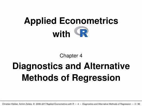
Applied Econometricswith
Chapter 4
Diagnostics and AlternativeMethods of Regression
Christian Kleiber, Achim Zeileis © 2008–2017Applied Econometrics with R – 4 – Diagnostics and Alternative Methods of Regression – 0 / 86
Diagnostics and Alternative Methods of Regression
Overview
Christian Kleiber, Achim Zeileis © 2008–2017Applied Econometrics with R – 4 – Diagnostics and Alternative Methods of Regression – 1 / 86
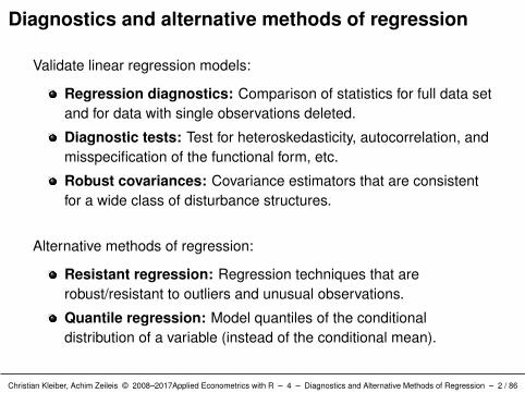
Diagnostics and alternative methods of regression
Validate linear regression models:
Regression diagnostics: Comparison of statistics for full data setand for data with single observations deleted.
Diagnostic tests: Test for heteroskedasticity, autocorrelation, andmisspecification of the functional form, etc.
Robust covariances: Covariance estimators that are consistentfor a wide class of disturbance structures.
Alternative methods of regression:
Resistant regression: Regression techniques that arerobust/resistant to outliers and unusual observations.
Quantile regression: Model quantiles of the conditionaldistribution of a variable (instead of the conditional mean).
Christian Kleiber, Achim Zeileis © 2008–2017Applied Econometrics with R – 4 – Diagnostics and Alternative Methods of Regression – 2 / 86
Diagnostics and Alternative Methods of Regression
Regression Diagnostics
Christian Kleiber, Achim Zeileis © 2008–2017Applied Econometrics with R – 4 – Diagnostics and Alternative Methods of Regression – 3 / 86
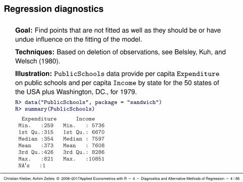
Regression diagnostics
Goal: Find points that are not fitted as well as they should be or haveundue influence on the fitting of the model.
Techniques: Based on deletion of observations, see Belsley, Kuh, andWelsch (1980).
Illustration: PublicSchools data provide per capita Expenditure
on public schools and per capita Income by state for the 50 states ofthe USA plus Washington, DC., for 1979.R> data("PublicSchools", package = "sandwich")R> summary(PublicSchools)
Expenditure IncomeMin. :259 Min. : 57361st Qu.:315 1st Qu.: 6670Median :354 Median : 7597Mean :373 Mean : 76083rd Qu.:426 3rd Qu.: 8286Max. :821 Max. :10851NA's :1
Christian Kleiber, Achim Zeileis © 2008–2017Applied Econometrics with R – 4 – Diagnostics and Alternative Methods of Regression – 4 / 86
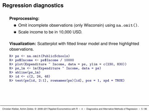
Regression diagnostics
Preprocessing:
Omit incomplete observations (only Wisconsin) using na.omit().
Scale income to be in 10,000 USD.
Visualization: Scatterplot with fitted linear model and three highlightedobservations.
R> ps <- na.omit(PublicSchools)R> ps$Income <- ps$Income / 10000R> plot(Expenditure ~ Income, data = ps, ylim = c(230, 830))R> ps_lm <- lm(Expenditure ~ Income, data = ps)R> abline(ps_lm)R> id <- c(2, 24, 48)R> text(ps[id, 2:1], rownames(ps)[id], pos = 1, xpd = TRUE)
Christian Kleiber, Achim Zeileis © 2008–2017Applied Econometrics with R – 4 – Diagnostics and Alternative Methods of Regression – 5 / 86
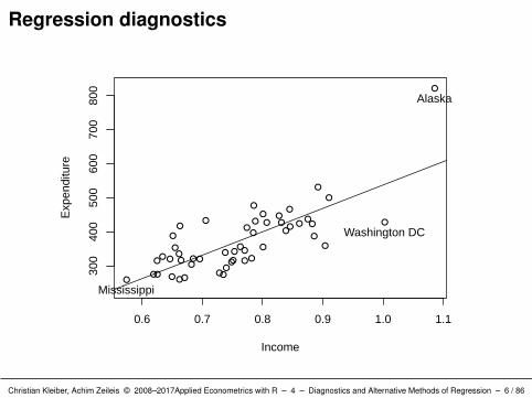
Regression diagnostics
0.6 0.7 0.8 0.9 1.0 1.1
300
400
500
600
700
800
Income
Exp
endi
ture
Alaska
Mississippi
Washington DC
Christian Kleiber, Achim Zeileis © 2008–2017Applied Econometrics with R – 4 – Diagnostics and Alternative Methods of Regression – 6 / 86
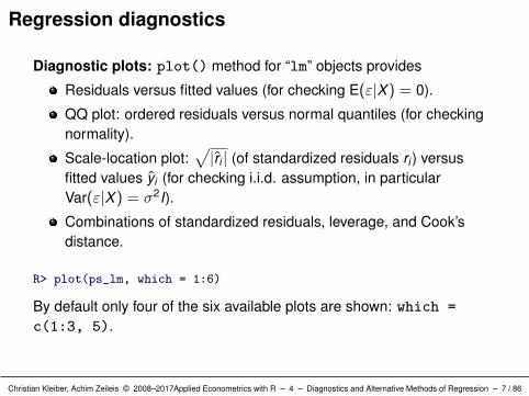
Regression diagnostics
Diagnostic plots: plot() method for “lm” objects provides
Residuals versus fitted values (for checking E(ε|X) = 0).
QQ plot: ordered residuals versus normal quantiles (for checkingnormality).
Scale-location plot:√|ri | (of standardized residuals ri ) versus
fitted values yi (for checking i.i.d. assumption, in particularVar(ε|X) = σ2I).
Combinations of standardized residuals, leverage, and Cook’sdistance.
R> plot(ps_lm, which = 1:6)
By default only four of the six available plots are shown: which =
c(1:3, 5).
Christian Kleiber, Achim Zeileis © 2008–2017Applied Econometrics with R – 4 – Diagnostics and Alternative Methods of Regression – 7 / 86
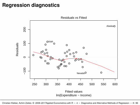
Regression diagnostics
250 300 350 400 450 500 550 600
−10
00
100
200
Fitted values
Res
idua
ls
lm(Expenditure ~ Income)
Residuals vs Fitted
Alaska
Nevada
Utah
Christian Kleiber, Achim Zeileis © 2008–2017Applied Econometrics with R – 4 – Diagnostics and Alternative Methods of Regression – 8 / 86
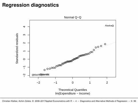
Regression diagnostics
−2 −1 0 1 2
−2
−1
01
23
4
Theoretical Quantiles
Sta
ndar
dize
d re
sidu
als
lm(Expenditure ~ Income)
Normal Q−Q
Alaska
Washington DCNevada
Christian Kleiber, Achim Zeileis © 2008–2017Applied Econometrics with R – 4 – Diagnostics and Alternative Methods of Regression – 9 / 86
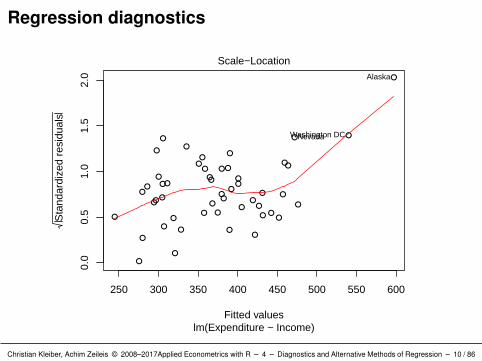
Regression diagnostics
250 300 350 400 450 500 550 600
0.0
0.5
1.0
1.5
2.0
Fitted values
Sta
ndar
dize
d re
sidu
als
lm(Expenditure ~ Income)
Scale−LocationAlaska
Washington DCNevada
Christian Kleiber, Achim Zeileis © 2008–2017Applied Econometrics with R – 4 – Diagnostics and Alternative Methods of Regression – 10 / 86
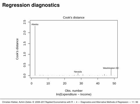
Regression diagnostics
0 10 20 30 40 50
0.0
0.5
1.0
1.5
2.0
2.5
Obs. number
Coo
k's
dist
ance
lm(Expenditure ~ Income)
Cook's distance
Alaska
Washington DC
Nevada
Christian Kleiber, Achim Zeileis © 2008–2017Applied Econometrics with R – 4 – Diagnostics and Alternative Methods of Regression – 11 / 86
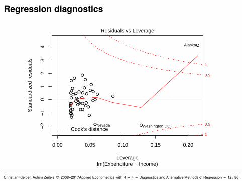
Regression diagnostics
0.00 0.05 0.10 0.15 0.20
−2
−1
01
23
4
Leverage
Sta
ndar
dize
d re
sidu
als
lm(Expenditure ~ Income)
Cook's distance1
0.5
0.5
1
Residuals vs Leverage
Alaska
Washington DCNevada
Christian Kleiber, Achim Zeileis © 2008–2017Applied Econometrics with R – 4 – Diagnostics and Alternative Methods of Regression – 12 / 86
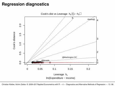
Regression diagnostics
0.0
0.5
1.0
1.5
2.0
Leverage hii
Coo
k's
dist
ance
0 0.05 0.1 0.15 0.2
lm(Expenditure ~ Income)
01
2
3
45
Cook's dist vs Leverage hii (1 − hii)
Alaska
Washington DC
Nevada
Christian Kleiber, Achim Zeileis © 2008–2017Applied Econometrics with R – 4 – Diagnostics and Alternative Methods of Regression – 13 / 86
Regression diagnostics
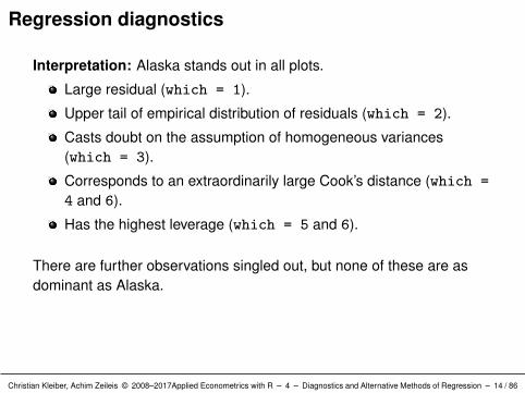
Interpretation: Alaska stands out in all plots.
Large residual (which = 1).
Upper tail of empirical distribution of residuals (which = 2).
Casts doubt on the assumption of homogeneous variances(which = 3).
Corresponds to an extraordinarily large Cook’s distance (which =
4 and 6).
Has the highest leverage (which = 5 and 6).
There are further observations singled out, but none of these are asdominant as Alaska.
Christian Kleiber, Achim Zeileis © 2008–2017Applied Econometrics with R – 4 – Diagnostics and Alternative Methods of Regression – 14 / 86
Leverage and standardized residuals
Recall: OLS residuals are not independent and do not have the samevariance.
More precisely: If Var(ε|X) = σ2I, then Var(ε|X) = σ2(I − H).H = X(X>X)−1X> is the “hat matrix”.
Hat values:
Diagonal elements hii of H.
Provided by generic function hatvalues().
Since Var(εi |X) = σ2(1− hii), observations with large hii will havesmall values of Var(εi |X), and hence tend to have residuals εi
close to zero.
hii measures the leverage of observation i .
Christian Kleiber, Achim Zeileis © 2008–2017Applied Econometrics with R – 4 – Diagnostics and Alternative Methods of Regression – 15 / 86
Leverage and standardized residuals
High leverage:
The trace of H is k (the number of regressors).
High leverage hii typically means two or three times larger thanaverage hat value k/n.
Leverage only depends on X and not on y .
Good/bad leverage points: high leverage points withtypical/unusual yi .
Visualize hat values with mean and three times the mean:
R> ps_hat <- hatvalues(ps_lm)R> plot(ps_hat)R> abline(h = c(1, 3) * mean(ps_hat), col = 2)R> id <- which(ps_hat > 3 * mean(ps_hat))R> text(id, ps_hat[id], rownames(ps)[id], pos = 1, xpd = TRUE)
Christian Kleiber, Achim Zeileis © 2008–2017Applied Econometrics with R – 4 – Diagnostics and Alternative Methods of Regression – 16 / 86
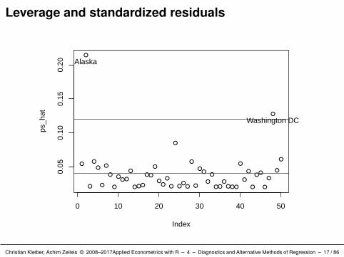
Leverage and standardized residuals
0 10 20 30 40 50
0.05
0.10
0.15
0.20
Index
ps_h
at
Alaska
Washington DC
Christian Kleiber, Achim Zeileis © 2008–2017Applied Econometrics with R – 4 – Diagnostics and Alternative Methods of Regression – 17 / 86
Leverage and standardized residuals
Standardized residuals: Var(εi |X) = σ2(1− hii) suggests
ri =εi
σ√
1− hii.
Sometimes referred to as “internally studentized residuals”.
Warning: not to be confused with (externally) studentized residuals(defined below).
If model assumptions are correct: Var(ri |X) = 1 and Cor(ri , rj |X)tends to be small.
In R: rstandard().
Christian Kleiber, Achim Zeileis © 2008–2017Applied Econometrics with R – 4 – Diagnostics and Alternative Methods of Regression – 18 / 86
Deletion diagnostics
Idea: Detection of unusual observations via leave-one-out (or deletion)diagnostics (see Belsley, Kuh, and Welsch 1980).
Notation: Exclude point i and compute
estimates β(i) and σ(i),
associated predictions y(i) = X β(i).
Influential observations: Observations whose removal causes a largechange in the fit.
Influential observations may or may not have large leverage and may ormay not be an outlier. But they tend to have at least one of theseproperties.
Christian Kleiber, Achim Zeileis © 2008–2017Applied Econometrics with R – 4 – Diagnostics and Alternative Methods of Regression – 19 / 86
Deletion diagnostics
Basic quantities:
DFFIT i = yi − yi,(i),
DFBETA = β − β(i),
COVRATIOi =det(σ2
(i)(X>(i)X(i))−1)
det(σ2(X>X)−1),
D2i =
(y − y(i))>(y − y(i))
k σ2 .
Interpretation:
DFFIT : change in fitted values (scaled version: DFFITS).
DFBETA: changes in coefficients (scaled version: DFBETAS).
COVRATIO: change in covariance matrix.
D2 (Cook’s distance): reduce information to a single value perobservation.
Christian Kleiber, Achim Zeileis © 2008–2017Applied Econometrics with R – 4 – Diagnostics and Alternative Methods of Regression – 20 / 86
Deletion diagnostics
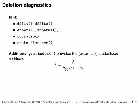
In R:
dffit(), dffits(),
dfbeta(), dfbetas(),
covratio(),
cooks.distance().
Additionally: rstudent() provides the (externally) studentizedresiduals
ti =εi
σ(i)√
1− hii .
Christian Kleiber, Achim Zeileis © 2008–2017Applied Econometrics with R – 4 – Diagnostics and Alternative Methods of Regression – 21 / 86
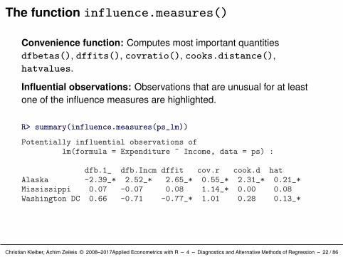
The function influence.measures()
Convenience function: Computes most important quantitiesdfbetas(), dffits(), covratio(), cooks.distance(),hatvalues.
Influential observations: Observations that are unusual for at leastone of the influence measures are highlighted.
R> summary(influence.measures(ps_lm))
Potentially influential observations oflm(formula = Expenditure ~ Income, data = ps) :
dfb.1_ dfb.Incm dffit cov.r cook.d hatAlaska -2.39_* 2.52_* 2.65_* 0.55_* 2.31_* 0.21_*Mississippi 0.07 -0.07 0.08 1.14_* 0.00 0.08Washington DC 0.66 -0.71 -0.77_* 1.01 0.28 0.13_*
Christian Kleiber, Achim Zeileis © 2008–2017Applied Econometrics with R – 4 – Diagnostics and Alternative Methods of Regression – 22 / 86
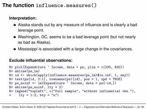
The function influence.measures()
Interpretation:
Alaska stands out by any measure of influence and is clearly a badleverage point.
Washington, DC, seems to be a bad leverage point (but not nearlyas bad as Alaska).
Mississippi is associated with a large change in the covariances.
Exclude influential observations:
R> plot(Expenditure ~ Income, data = ps, ylim = c(230, 830))R> abline(ps_lm)R> id <- which(apply(influence.measures(ps_lm)$is.inf, 1, any))R> text(ps[id, 2:1], rownames(ps)[id], pos = 1, xpd = TRUE)R> ps_noinf <- lm(Expenditure ~ Income, data = ps[-id,])R> abline(ps_noinf, lty = 2)R> legend("topleft", c("full sample", "without influential obs."),+ lty = 1:2, bty = "n")
Christian Kleiber, Achim Zeileis © 2008–2017Applied Econometrics with R – 4 – Diagnostics and Alternative Methods of Regression – 23 / 86
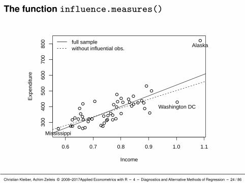
The function influence.measures()
0.6 0.7 0.8 0.9 1.0 1.1
300
400
500
600
700
800
Income
Exp
endi
ture
Alaska
Mississippi
Washington DC
full samplewithout influential obs.
Christian Kleiber, Achim Zeileis © 2008–2017Applied Econometrics with R – 4 – Diagnostics and Alternative Methods of Regression – 24 / 86
Diagnostics and Alternative Methods of Regression
Diagnostic Tests
Christian Kleiber, Achim Zeileis © 2008–2017Applied Econometrics with R – 4 – Diagnostics and Alternative Methods of Regression – 25 / 86
Diagnostics tests
More formal validation: Diagnostic testing, e.g., for heteroskedasticityin cross-section regressions or disturbance autocorrelation in timeseries regressions.
In R: Package lmtest provides a large collection of diagnostic tests.
Typically, the tests return an object of class “htest” (hypothesis test)with test statistic, corresponding p value, and additional parameterssuch as degrees of freedom (where appropriate), the name of thetested model, or the method used.
Background: Underlying theory is provided in Baltagi (2002), Davidsonand MacKinnon (2004), and Greene (2003).
Christian Kleiber, Achim Zeileis © 2008–2017Applied Econometrics with R – 4 – Diagnostics and Alternative Methods of Regression – 26 / 86
Diagnostics tests
Illustration: Reconsider Journals data as an example forcross-section regressions.
Preprocessing: As before and additionally include age of the journals(for the year 2000, when the data were collected).
R> data("Journals", package = "AER")R> journals <- Journals[, c("subs", "price")]R> journals$citeprice <- Journals$price/Journals$citationsR> journals$age <- 2000 - Journals$foundingyear
Regression: log-subscriptions explained by log-price per citation.
R> jour_lm <- lm(log(subs) ~ log(citeprice), data = journals)
Christian Kleiber, Achim Zeileis © 2008–2017Applied Econometrics with R – 4 – Diagnostics and Alternative Methods of Regression – 27 / 86
Testing for heteroskedasticity
Assumption of homoskedasticity Var(εi |xi) = σ2 must be checked incross-section regressions.
Breusch-Pagan test:
Fit linear regression model to the squared residuals ε2i .
Reject if too much of the variance is explained by additionalexplanatory variables, e.g.,
Original regressors X (as in the main model).Original regressors plus squared terms and interactions.
Illustration: For jour_lm, variance seems to decreases with the fittedvalues, or, equivalently, increases with log(citeprice).
Null distribution: Approximately χ2q , where q is the number of auxiliary
regressors (excluding constant term).
Christian Kleiber, Achim Zeileis © 2008–2017Applied Econometrics with R – 4 – Diagnostics and Alternative Methods of Regression – 28 / 86
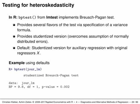
Testing for heteroskedasticity
In R: bptest() from lmtest implements Breusch-Pagan test.
Provides several flavors of the test via specification of a varianceformula.
Provides studentized version (overcomes assumption of normallydistributed errors).
Default: Studentized version for auxiliary regression with originalregressors X .
Example using defaults
R> bptest(jour_lm)
studentized Breusch-Pagan test
data: jour_lmBP = 9.8, df = 1, p-value = 0.002
Christian Kleiber, Achim Zeileis © 2008–2017Applied Econometrics with R – 4 – Diagnostics and Alternative Methods of Regression – 29 / 86
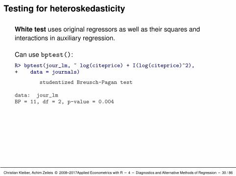
Testing for heteroskedasticity
White test uses original regressors as well as their squares andinteractions in auxiliary regression.
Can use bptest():
R> bptest(jour_lm, ~ log(citeprice) + I(log(citeprice)^2),+ data = journals)
studentized Breusch-Pagan test
data: jour_lmBP = 11, df = 2, p-value = 0.004
Christian Kleiber, Achim Zeileis © 2008–2017Applied Econometrics with R – 4 – Diagnostics and Alternative Methods of Regression – 30 / 86
Testing for heteroskedasticity
Goldfeld-Quandt test:
Nowadays probably more popular in textbooks than in appliedwork.
Order sample with respect to the variable explaining theheteroskedasticity (in example: price per citation).
Split sample and compare mean residual sum of squares beforeand after the split point via an F test.
Problem: A meaningful split point is rarely known in advance.
Modification: Omit some central observations to improve thepower.
Christian Kleiber, Achim Zeileis © 2008–2017Applied Econometrics with R – 4 – Diagnostics and Alternative Methods of Regression – 31 / 86
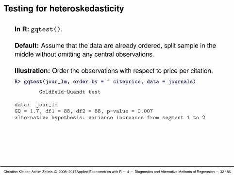
Testing for heteroskedasticity
In R: gqtest().
Default: Assume that the data are already ordered, split sample in themiddle without omitting any central observations.
Illustration: Order the observations with respect to price per citation.
R> gqtest(jour_lm, order.by = ~ citeprice, data = journals)
Goldfeld-Quandt test
data: jour_lmGQ = 1.7, df1 = 88, df2 = 88, p-value = 0.007alternative hypothesis: variance increases from segment 1 to 2
Christian Kleiber, Achim Zeileis © 2008–2017Applied Econometrics with R – 4 – Diagnostics and Alternative Methods of Regression – 32 / 86
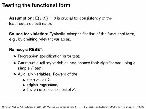
Testing the functional form
Assumption: E(ε|X) = 0 is crucial for consistency of theleast-squares estimator.
Source for violation: Typically, misspecification of the functional form,e.g., by omitting relevant variables.
Ramsey’s RESET:
Regression specification error test.
Construct auxiliary variables and assess their significance using asimple F test.Auxiliary variables: Powers of the
fitted values y ,original regressors,first principal component of X .
Christian Kleiber, Achim Zeileis © 2008–2017Applied Econometrics with R – 4 – Diagnostics and Alternative Methods of Regression – 33 / 86
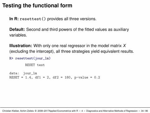
Testing the functional form
In R: resettest() provides all three versions.
Default: Second and third powers of the fitted values as auxiliaryvariables.
Illustration: With only one real regressor in the model matrix X(excluding the intercept), all three strategies yield equivalent results.
R> resettest(jour_lm)
RESET test
data: jour_lmRESET = 1.4, df1 = 2, df2 = 180, p-value = 0.2
Christian Kleiber, Achim Zeileis © 2008–2017Applied Econometrics with R – 4 – Diagnostics and Alternative Methods of Regression – 34 / 86
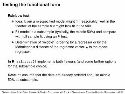
Testing the functional form
Rainbow test:
Idea: Even a misspecified model might fit (reasonably) well in the“center” of the sample but might lack fit in the tails.
Fit model to a subsample (typically, the middle 50%) and comparewith full sample fit using an F test.
Determination of “middle”: ordering by a regressor or by theMahalanobis distance of the regressor vector xi to the meanregressor.
In R: raintest() implements both flavours (and some further optionsfor the subsample choice).
Default: Assume that the data are already ordered and use middle50% as subsample.
Christian Kleiber, Achim Zeileis © 2008–2017Applied Econometrics with R – 4 – Diagnostics and Alternative Methods of Regression – 35 / 86

Testing the functional form
Illustration: Assess stability of functional form over age of journals.
R> raintest(jour_lm, order.by = ~ age, data = journals)
Rainbow test
data: jour_lmRain = 1.8, df1 = 90, df2 = 88, p-value = 0.004
Interpretation:
The fit for the 50% “middle-aged” journals is significantly differentfrom the fit comprising all journals.
Relationship between the number of subscriptions and the priceper citation also depends on the age of the journal.
As we will see below: Libraries are willing to pay more forestablished journals.
Christian Kleiber, Achim Zeileis © 2008–2017Applied Econometrics with R – 4 – Diagnostics and Alternative Methods of Regression – 36 / 86
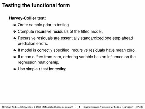
Testing the functional form
Harvey-Collier test:
Order sample prior to testing.
Compute recursive residuals of the fitted model.
Recursive residuals are essentially standardized one-step-aheadprediction errors.
If model is correctly specified, recursive residuals have mean zero.
If mean differs from zero, ordering variable has an influence on theregression relationship.
Use simple t test for testing.
Christian Kleiber, Achim Zeileis © 2008–2017Applied Econometrics with R – 4 – Diagnostics and Alternative Methods of Regression – 37 / 86
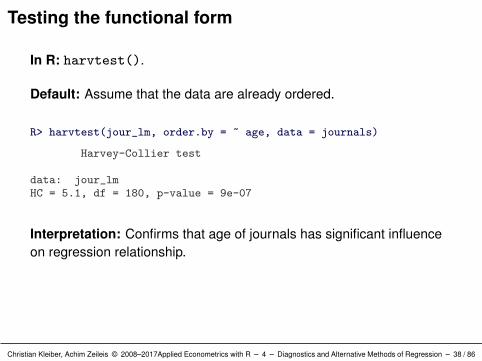
Testing the functional form
In R: harvtest().
Default: Assume that the data are already ordered.
R> harvtest(jour_lm, order.by = ~ age, data = journals)
Harvey-Collier test
data: jour_lmHC = 5.1, df = 180, p-value = 9e-07
Interpretation: Confirms that age of journals has significant influenceon regression relationship.
Christian Kleiber, Achim Zeileis © 2008–2017Applied Econometrics with R – 4 – Diagnostics and Alternative Methods of Regression – 38 / 86
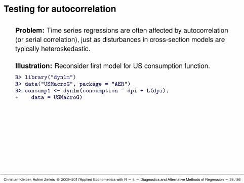
Testing for autocorrelation
Problem: Time series regressions are often affected by autocorrelation(or serial correlation), just as disturbances in cross-section models aretypically heteroskedastic.
Illustration: Reconsider first model for US consumption function.
R> library("dynlm")R> data("USMacroG", package = "AER")R> consump1 <- dynlm(consumption ~ dpi + L(dpi),+ data = USMacroG)
Christian Kleiber, Achim Zeileis © 2008–2017Applied Econometrics with R – 4 – Diagnostics and Alternative Methods of Regression – 39 / 86
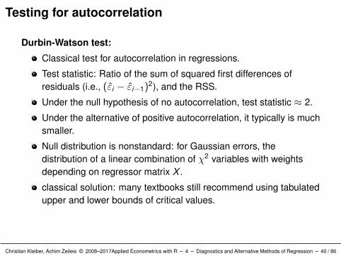
Testing for autocorrelation
Durbin-Watson test:
Classical test for autocorrelation in regressions.
Test statistic: Ratio of the sum of squared first differences ofresiduals (i.e., (εi − εi−1)2), and the RSS.
Under the null hypothesis of no autocorrelation, test statistic ≈ 2.
Under the alternative of positive autocorrelation, it typically is muchsmaller.
Null distribution is nonstandard: for Gaussian errors, thedistribution of a linear combination of χ2 variables with weightsdepending on regressor matrix X .
classical solution: many textbooks still recommend using tabulatedupper and lower bounds of critical values.
Christian Kleiber, Achim Zeileis © 2008–2017Applied Econometrics with R – 4 – Diagnostics and Alternative Methods of Regression – 40 / 86
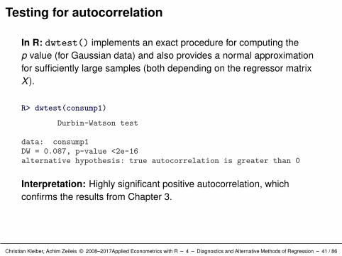
Testing for autocorrelation
In R: dwtest() implements an exact procedure for computing thep value (for Gaussian data) and also provides a normal approximationfor sufficiently large samples (both depending on the regressor matrixX ).
R> dwtest(consump1)
Durbin-Watson test
data: consump1DW = 0.087, p-value <2e-16alternative hypothesis: true autocorrelation is greater than 0
Interpretation: Highly significant positive autocorrelation, whichconfirms the results from Chapter 3.
Christian Kleiber, Achim Zeileis © 2008–2017Applied Econometrics with R – 4 – Diagnostics and Alternative Methods of Regression – 41 / 86
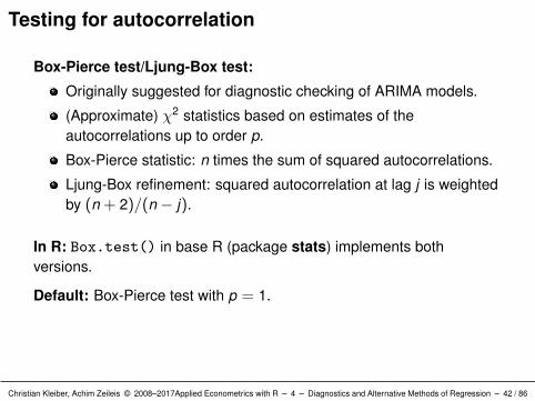
Testing for autocorrelation
Box-Pierce test/Ljung-Box test:
Originally suggested for diagnostic checking of ARIMA models.
(Approximate) χ2 statistics based on estimates of theautocorrelations up to order p.
Box-Pierce statistic: n times the sum of squared autocorrelations.
Ljung-Box refinement: squared autocorrelation at lag j is weightedby (n + 2)/(n − j).
In R: Box.test() in base R (package stats) implements bothversions.
Default: Box-Pierce test with p = 1.
Christian Kleiber, Achim Zeileis © 2008–2017Applied Econometrics with R – 4 – Diagnostics and Alternative Methods of Regression – 42 / 86
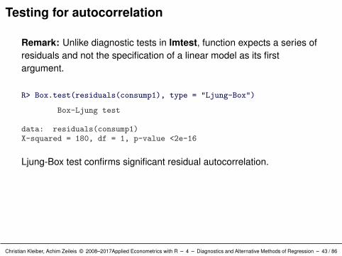
Testing for autocorrelation
Remark: Unlike diagnostic tests in lmtest, function expects a series ofresiduals and not the specification of a linear model as its firstargument.
R> Box.test(residuals(consump1), type = "Ljung-Box")
Box-Ljung test
data: residuals(consump1)X-squared = 180, df = 1, p-value <2e-16
Ljung-Box test confirms significant residual autocorrelation.
Christian Kleiber, Achim Zeileis © 2008–2017Applied Econometrics with R – 4 – Diagnostics and Alternative Methods of Regression – 43 / 86
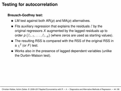
Testing for autocorrelation
Breusch-Godfrey test:
LM test against both AR(p) and MA(p) alternatives.
Fits auxiliary regression that explains the residuals ε by theoriginal regressors X augmented by the lagged residuals up toorder p (εi−1, . . . , εi−p) (where zeros are used as starting values).
The resulting RSS is compared with the RSS of the original RSS ina χ2 (or F ) test.
Works also in the presence of lagged dependent variables (unlikethe Durbin-Watson test).
Christian Kleiber, Achim Zeileis © 2008–2017Applied Econometrics with R – 4 – Diagnostics and Alternative Methods of Regression – 44 / 86
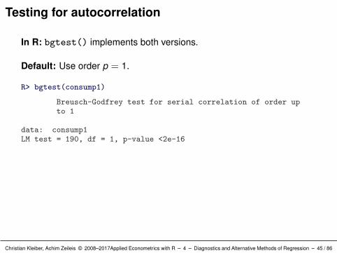
Testing for autocorrelation
In R: bgtest() implements both versions.
Default: Use order p = 1.
R> bgtest(consump1)
Breusch-Godfrey test for serial correlation of order upto 1
data: consump1LM test = 190, df = 1, p-value <2e-16
Christian Kleiber, Achim Zeileis © 2008–2017Applied Econometrics with R – 4 – Diagnostics and Alternative Methods of Regression – 45 / 86
Diagnostics and Alternative Methods of Regression
Robust Standard Errors and Tests
Christian Kleiber, Achim Zeileis © 2008–2017Applied Econometrics with R – 4 – Diagnostics and Alternative Methods of Regression – 46 / 86
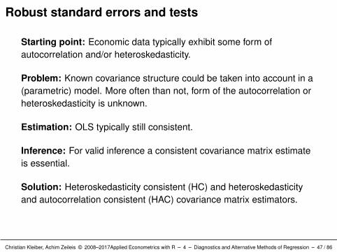
Robust standard errors and tests
Starting point: Economic data typically exhibit some form ofautocorrelation and/or heteroskedasticity.
Problem: Known covariance structure could be taken into account in a(parametric) model. More often than not, form of the autocorrelation orheteroskedasticity is unknown.
Estimation: OLS typically still consistent.
Inference: For valid inference a consistent covariance matrix estimateis essential.
Solution: Heteroskedasticity consistent (HC) and heteroskedasticityand autocorrelation consistent (HAC) covariance matrix estimators.
Christian Kleiber, Achim Zeileis © 2008–2017Applied Econometrics with R – 4 – Diagnostics and Alternative Methods of Regression – 47 / 86
Robust standard errors and tests
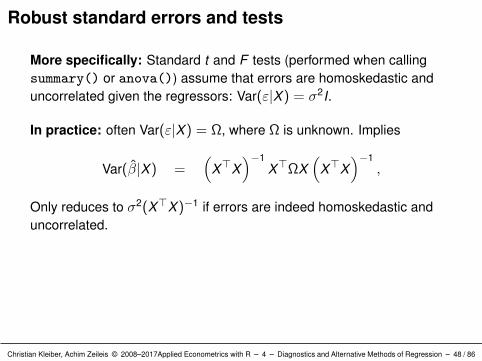
More specifically: Standard t and F tests (performed when callingsummary() or anova()) assume that errors are homoskedastic anduncorrelated given the regressors: Var(ε|X) = σ2I.
In practice: often Var(ε|X) = Ω, where Ω is unknown. Implies
Var(β|X) =(
X>X)−1
X>ΩX(
X>X)−1
,
Only reduces to σ2(X>X)−1 if errors are indeed homoskedastic anduncorrelated.
Christian Kleiber, Achim Zeileis © 2008–2017Applied Econometrics with R – 4 – Diagnostics and Alternative Methods of Regression – 48 / 86
Robust standard errors and tests
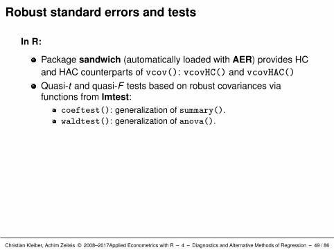
In R:
Package sandwich (automatically loaded with AER) provides HCand HAC counterparts of vcov(): vcovHC() and vcovHAC()
Quasi-t and quasi-F tests based on robust covariances viafunctions from lmtest:
coeftest(): generalization of summary().waldtest(): generalization of anova().
Christian Kleiber, Achim Zeileis © 2008–2017Applied Econometrics with R – 4 – Diagnostics and Alternative Methods of Regression – 49 / 86
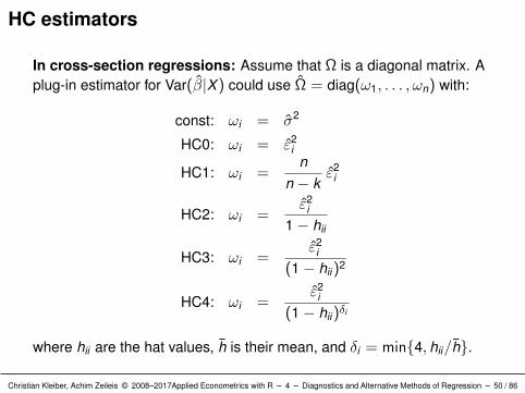
HC estimators
In cross-section regressions: Assume that Ω is a diagonal matrix. Aplug-in estimator for Var(β|X) could use Ω = diag(ω1, . . . , ωn) with:
const: ωi = σ2
HC0: ωi = ε2i
HC1: ωi =n
n − kε2
i
HC2: ωi =ε2
i
1− hii
HC3: ωi =ε2
i
(1− hii)2
HC4: ωi =ε2
i
(1− hii)δi
where hii are the hat values, h is their mean, and δi = min4, hii/h.
Christian Kleiber, Achim Zeileis © 2008–2017Applied Econometrics with R – 4 – Diagnostics and Alternative Methods of Regression – 50 / 86
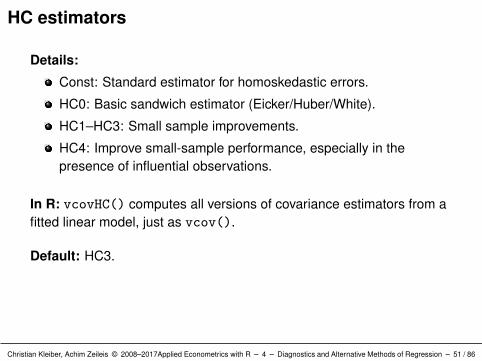
HC estimators
Details:
Const: Standard estimator for homoskedastic errors.
HC0: Basic sandwich estimator (Eicker/Huber/White).
HC1–HC3: Small sample improvements.
HC4: Improve small-sample performance, especially in thepresence of influential observations.
In R: vcovHC() computes all versions of covariance estimators from afitted linear model, just as vcov().
Default: HC3.
Christian Kleiber, Achim Zeileis © 2008–2017Applied Econometrics with R – 4 – Diagnostics and Alternative Methods of Regression – 51 / 86
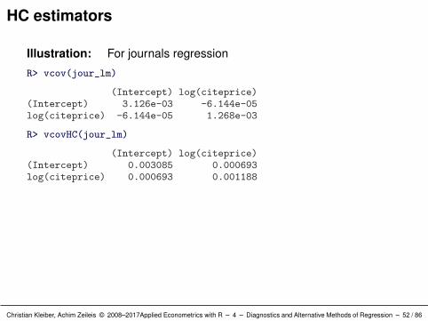
HC estimators
Illustration: For journals regression
R> vcov(jour_lm)
(Intercept) log(citeprice)(Intercept) 3.126e-03 -6.144e-05log(citeprice) -6.144e-05 1.268e-03
R> vcovHC(jour_lm)
(Intercept) log(citeprice)(Intercept) 0.003085 0.000693log(citeprice) 0.000693 0.001188
Christian Kleiber, Achim Zeileis © 2008–2017Applied Econometrics with R – 4 – Diagnostics and Alternative Methods of Regression – 52 / 86
HC estimators
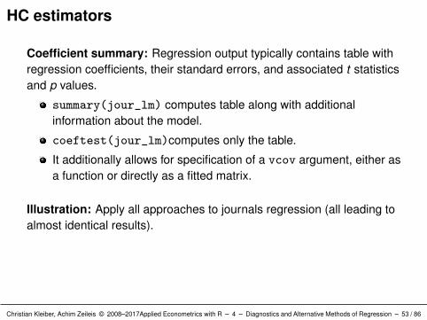
Coefficient summary: Regression output typically contains table withregression coefficients, their standard errors, and associated t statisticsand p values.
summary(jour_lm) computes table along with additionalinformation about the model.
coeftest(jour_lm)computes only the table.
It additionally allows for specification of a vcov argument, either asa function or directly as a fitted matrix.
Illustration: Apply all approaches to journals regression (all leading toalmost identical results).
Christian Kleiber, Achim Zeileis © 2008–2017Applied Econometrics with R – 4 – Diagnostics and Alternative Methods of Regression – 53 / 86
HC estimators
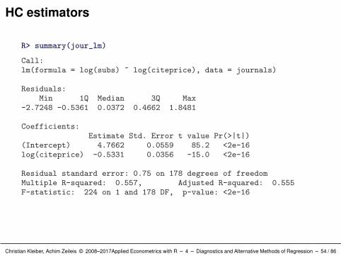
R> summary(jour_lm)
Call:lm(formula = log(subs) ~ log(citeprice), data = journals)
Residuals:Min 1Q Median 3Q Max
-2.7248 -0.5361 0.0372 0.4662 1.8481
Coefficients:Estimate Std. Error t value Pr(>|t|)
(Intercept) 4.7662 0.0559 85.2 <2e-16log(citeprice) -0.5331 0.0356 -15.0 <2e-16
Residual standard error: 0.75 on 178 degrees of freedomMultiple R-squared: 0.557, Adjusted R-squared: 0.555F-statistic: 224 on 1 and 178 DF, p-value: <2e-16
Christian Kleiber, Achim Zeileis © 2008–2017Applied Econometrics with R – 4 – Diagnostics and Alternative Methods of Regression – 54 / 86
HC estimators
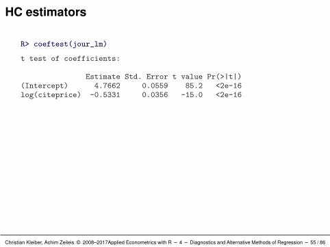
R> coeftest(jour_lm)
t test of coefficients:
Estimate Std. Error t value Pr(>|t|)(Intercept) 4.7662 0.0559 85.2 <2e-16log(citeprice) -0.5331 0.0356 -15.0 <2e-16
Christian Kleiber, Achim Zeileis © 2008–2017Applied Econometrics with R – 4 – Diagnostics and Alternative Methods of Regression – 55 / 86
HC estimators
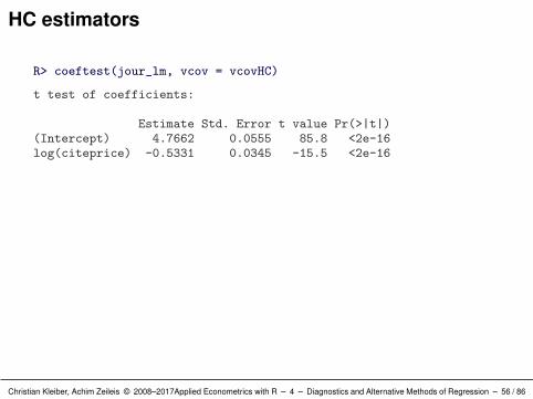
R> coeftest(jour_lm, vcov = vcovHC)
t test of coefficients:
Estimate Std. Error t value Pr(>|t|)(Intercept) 4.7662 0.0555 85.8 <2e-16log(citeprice) -0.5331 0.0345 -15.5 <2e-16
Christian Kleiber, Achim Zeileis © 2008–2017Applied Econometrics with R – 4 – Diagnostics and Alternative Methods of Regression – 56 / 86
HC estimators
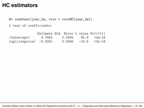
R> coeftest(jour_lm, vcov = vcovHC(jour_lm))
t test of coefficients:
Estimate Std. Error t value Pr(>|t|)(Intercept) 4.7662 0.0555 85.8 <2e-16log(citeprice) -0.5331 0.0345 -15.5 <2e-16
Christian Kleiber, Achim Zeileis © 2008–2017Applied Econometrics with R – 4 – Diagnostics and Alternative Methods of Regression – 57 / 86
HC estimators
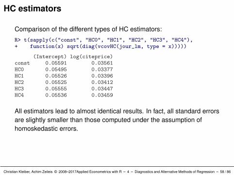
Comparison of the different types of HC estimators:
R> t(sapply(c("const", "HC0", "HC1", "HC2", "HC3", "HC4"),+ function(x) sqrt(diag(vcovHC(jour_lm, type = x)))))
(Intercept) log(citeprice)const 0.05591 0.03561HC0 0.05495 0.03377HC1 0.05526 0.03396HC2 0.05525 0.03412HC3 0.05555 0.03447HC4 0.05536 0.03459
All estimators lead to almost identical results. In fact, all standard errorsare slightly smaller than those computed under the assumption ofhomoskedastic errors.
Christian Kleiber, Achim Zeileis © 2008–2017Applied Econometrics with R – 4 – Diagnostics and Alternative Methods of Regression – 58 / 86
HC estimators
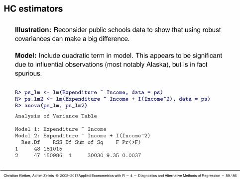
Illustration: Reconsider public schools data to show that using robustcovariances can make a big difference.
Model: Include quadratic term in model. This appears to be significantdue to influential observations (most notably Alaska), but is in factspurious.
R> ps_lm <- lm(Expenditure ~ Income, data = ps)R> ps_lm2 <- lm(Expenditure ~ Income + I(Income^2), data = ps)R> anova(ps_lm, ps_lm2)
Analysis of Variance Table
Model 1: Expenditure ~ IncomeModel 2: Expenditure ~ Income + I(Income^2)Res.Df RSS Df Sum of Sq F Pr(>F)
1 48 1810152 47 150986 1 30030 9.35 0.0037
Christian Kleiber, Achim Zeileis © 2008–2017Applied Econometrics with R – 4 – Diagnostics and Alternative Methods of Regression – 59 / 86
HC estimators
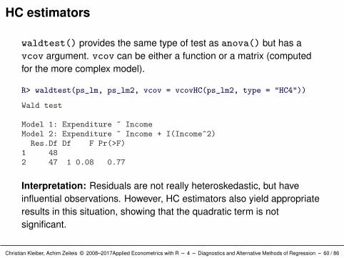
waldtest() provides the same type of test as anova() but has avcov argument. vcov can be either a function or a matrix (computedfor the more complex model).
R> waldtest(ps_lm, ps_lm2, vcov = vcovHC(ps_lm2, type = "HC4"))
Wald test
Model 1: Expenditure ~ IncomeModel 2: Expenditure ~ Income + I(Income^2)Res.Df Df F Pr(>F)
1 482 47 1 0.08 0.77
Interpretation: Residuals are not really heteroskedastic, but haveinfluential observations. However, HC estimators also yield appropriateresults in this situation, showing that the quadratic term is notsignificant.
Christian Kleiber, Achim Zeileis © 2008–2017Applied Econometrics with R – 4 – Diagnostics and Alternative Methods of Regression – 60 / 86
HAC estimators
In time series regressions: If the error terms εi are correlated, Ω isnot diagonal and can only be estimated directly upon introducing furtherassumptions on its structure.
Solution: If form of heteroskedasticity and autocorrelation is unknown,valid standard errors and tests may be obtained by estimating X>ΩXinstead.
Technically: Computing weighted sums of the empiricalautocorrelations of εixi .
Estimators: Differ with respect to choice of weights.
Choice of weights: Based on different kernel functions and bandwidthselection strategies.
Christian Kleiber, Achim Zeileis © 2008–2017Applied Econometrics with R – 4 – Diagnostics and Alternative Methods of Regression – 61 / 86
HAC estimators
In R: vcovHAC() provides general framework for HAC estimators.
Convenience interfaces:
NeweyWest() (by default) uses a Bartlett kernel withnonparametric bandwidth selection (Newey and West 1987, 1994).
kernHAC() (by default) uses a quadratic spectral kernel withparametric bandwidth selection (Andrews 1991, Andrews andMonahan 1992).
Both use prewhitening (by default).
weave() implements the class of weighted empirical adaptivevariance estimators (Lumley and Heagerty 1999).
Illustration: Newey-West and Andrews kernel HAC estimators forconsumption function regression.
Christian Kleiber, Achim Zeileis © 2008–2017Applied Econometrics with R – 4 – Diagnostics and Alternative Methods of Regression – 62 / 86
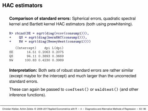
HAC estimators
Comparison of standard errors: Spherical errors, quadratic spectralkernel and Bartlett kernel HAC estimators (both using prewhitening).
R> rbind(SE = sqrt(diag(vcov(consump1))),+ QS = sqrt(diag(kernHAC(consump1))),+ NW = sqrt(diag(NeweyWest(consump1))))
(Intercept) dpi L(dpi)SE 14.51 0.2063 0.2075QS 94.11 0.3893 0.3669NW 100.83 0.4230 0.3989
Interpretation: Both sets of robust standard errors are rather similar(except maybe for the intercept) and much larger than the uncorrectedstandard errors.
These can again be passed to coeftest() or waldtest() (and otherinference functions).
Christian Kleiber, Achim Zeileis © 2008–2017Applied Econometrics with R – 4 – Diagnostics and Alternative Methods of Regression – 63 / 86
Diagnostics and Alternative Methods of Regression
Resistant Regression
Christian Kleiber, Achim Zeileis © 2008–2017Applied Econometrics with R – 4 – Diagnostics and Alternative Methods of Regression – 64 / 86
Resistant regression
Goal: Regression that is “resistant” (or “robust”) to a (small) group ofoutlying observations.
Previously: Leave-one-out (deletion) diagnostics.
Problem: Outliers of the same type can mask each other inleave-one-out diagnostics.
Solution: In low-dimensional problems, use plotting. Inhigh-dimensional data, use regressions that withstand alterations in acertain percentage of the data.
Estimators: Least median of squares (LMS) and least trimmedsquares (LTS) regression.
Christian Kleiber, Achim Zeileis © 2008–2017Applied Econometrics with R – 4 – Diagnostics and Alternative Methods of Regression – 65 / 86
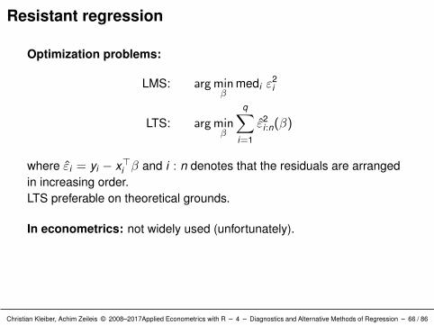
Resistant regression
Optimization problems:
LMS: arg minβ
medi ε2i
LTS: arg minβ
q∑i=1
ε2i:n(β)
where εi = yi − x>i β and i : n denotes that the residuals are arrangedin increasing order.LTS preferable on theoretical grounds.
In econometrics: not widely used (unfortunately).
Christian Kleiber, Achim Zeileis © 2008–2017Applied Econometrics with R – 4 – Diagnostics and Alternative Methods of Regression – 66 / 86
Resistant regression
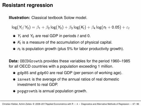
Illustration: Classical textbook Solow model.
log(Yt/Y0) = β1 + β2 log(Y0) + β3 log(Kt) + β4 log(nt + 0.05) + εt
Yt and Y0 are real GDP in periods t and 0.
Kt is a measure of the accumulation of physical capital.
nt is population growth (plus 5% for labor productivity growth).
Data: OECDGrowth provides these variables for the period 1960–1985for all OECD countries with a population exceeding 1 million.
gdp85 and gdp60 are real GDP (per person of working age).
invest is the average of the annual ratios of real domesticinvestment to real GDP.
popgrowth is annual population growth.
Christian Kleiber, Achim Zeileis © 2008–2017Applied Econometrics with R – 4 – Diagnostics and Alternative Methods of Regression – 67 / 86
Resistant regression
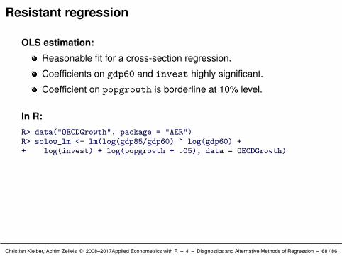
OLS estimation:
Reasonable fit for a cross-section regression.
Coefficients on gdp60 and invest highly significant.
Coefficient on popgrowth is borderline at 10% level.
In R:
R> data("OECDGrowth", package = "AER")R> solow_lm <- lm(log(gdp85/gdp60) ~ log(gdp60) ++ log(invest) + log(popgrowth + .05), data = OECDGrowth)
Christian Kleiber, Achim Zeileis © 2008–2017Applied Econometrics with R – 4 – Diagnostics and Alternative Methods of Regression – 68 / 86
Resistant regression
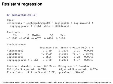
R> summary(solow_lm)
Call:lm(formula = log(gdp85/gdp60) ~ log(gdp60) + log(invest) +
log(popgrowth + 0.05), data = OECDGrowth)
Residuals:Min 1Q Median 3Q Max
-0.1840 -0.0399 -0.0078 0.0451 0.3188
Coefficients:Estimate Std. Error t value Pr(>|t|)
(Intercept) 2.9759 1.0216 2.91 0.0093log(gdp60) -0.3429 0.0565 -6.07 9.8e-06log(invest) 0.6501 0.2020 3.22 0.0048log(popgrowth + 0.05) -0.5730 0.2904 -1.97 0.0640
Residual standard error: 0.133 on 18 degrees of freedomMultiple R-squared: 0.746, Adjusted R-squared: 0.704F-statistic: 17.7 on 3 and 18 DF, p-value: 1.34e-05
Christian Kleiber, Achim Zeileis © 2008–2017Applied Econometrics with R – 4 – Diagnostics and Alternative Methods of Regression – 69 / 86
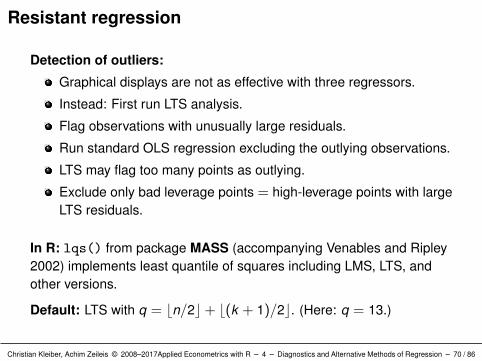
Resistant regression
Detection of outliers:
Graphical displays are not as effective with three regressors.
Instead: First run LTS analysis.
Flag observations with unusually large residuals.
Run standard OLS regression excluding the outlying observations.
LTS may flag too many points as outlying.
Exclude only bad leverage points = high-leverage points with largeLTS residuals.
In R: lqs() from package MASS (accompanying Venables and Ripley2002) implements least quantile of squares including LMS, LTS, andother versions.
Default: LTS with q = bn/2c+ b(k + 1)/2c. (Here: q = 13.)
Christian Kleiber, Achim Zeileis © 2008–2017Applied Econometrics with R – 4 – Diagnostics and Alternative Methods of Regression – 70 / 86
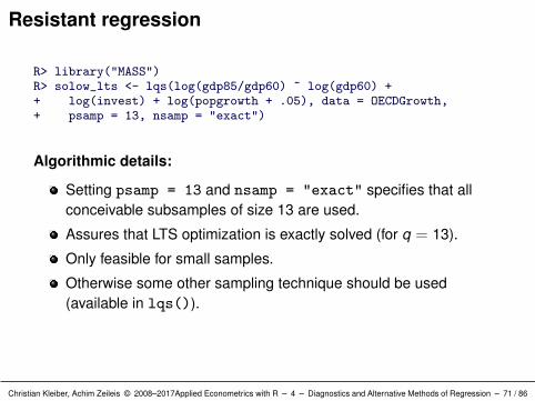
Resistant regression
R> library("MASS")R> solow_lts <- lqs(log(gdp85/gdp60) ~ log(gdp60) ++ log(invest) + log(popgrowth + .05), data = OECDGrowth,+ psamp = 13, nsamp = "exact")
Algorithmic details:
Setting psamp = 13 and nsamp = "exact" specifies that allconceivable subsamples of size 13 are used.
Assures that LTS optimization is exactly solved (for q = 13).
Only feasible for small samples.
Otherwise some other sampling technique should be used(available in lqs()).
Christian Kleiber, Achim Zeileis © 2008–2017Applied Econometrics with R – 4 – Diagnostics and Alternative Methods of Regression – 71 / 86
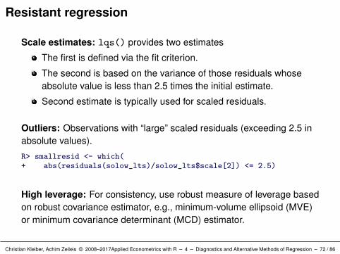
Resistant regression
Scale estimates: lqs() provides two estimates
The first is defined via the fit criterion.
The second is based on the variance of those residuals whoseabsolute value is less than 2.5 times the initial estimate.
Second estimate is typically used for scaled residuals.
Outliers: Observations with “large” scaled residuals (exceeding 2.5 inabsolute values).
R> smallresid <- which(+ abs(residuals(solow_lts)/solow_lts$scale[2]) <= 2.5)
High leverage: For consistency, use robust measure of leverage basedon robust covariance estimator, e.g., minimum-volume ellipsoid (MVE)or minimum covariance determinant (MCD) estimator.
Christian Kleiber, Achim Zeileis © 2008–2017Applied Econometrics with R – 4 – Diagnostics and Alternative Methods of Regression – 72 / 86
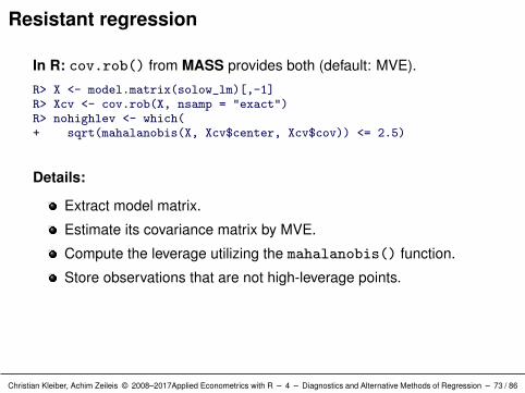
Resistant regression
In R: cov.rob() from MASS provides both (default: MVE).
R> X <- model.matrix(solow_lm)[,-1]R> Xcv <- cov.rob(X, nsamp = "exact")R> nohighlev <- which(+ sqrt(mahalanobis(X, Xcv$center, Xcv$cov)) <= 2.5)
Details:
Extract model matrix.
Estimate its covariance matrix by MVE.
Compute the leverage utilizing the mahalanobis() function.
Store observations that are not high-leverage points.
Christian Kleiber, Achim Zeileis © 2008–2017Applied Econometrics with R – 4 – Diagnostics and Alternative Methods of Regression – 73 / 86
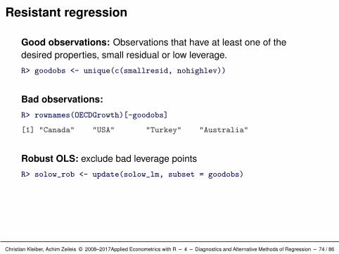
Resistant regression
Good observations: Observations that have at least one of thedesired properties, small residual or low leverage.
R> goodobs <- unique(c(smallresid, nohighlev))
Bad observations:
R> rownames(OECDGrowth)[-goodobs]
[1] "Canada" "USA" "Turkey" "Australia"
Robust OLS: exclude bad leverage points
R> solow_rob <- update(solow_lm, subset = goodobs)
Christian Kleiber, Achim Zeileis © 2008–2017Applied Econometrics with R – 4 – Diagnostics and Alternative Methods of Regression – 74 / 86
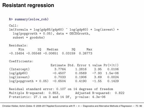
Resistant regression
R> summary(solow_rob)
Call:lm(formula = log(gdp85/gdp60) ~ log(gdp60) + log(invest) +
log(popgrowth + 0.05), data = OECDGrowth,subset = goodobs)
Residuals:Min 1Q Median 3Q Max
-0.15454 -0.05548 -0.00651 0.03159 0.26773
Coefficients:Estimate Std. Error t value Pr(>|t|)
(Intercept) 3.7764 1.2816 2.95 0.0106log(gdp60) -0.4507 0.0569 -7.93 1.5e-06log(invest) 0.7033 0.1906 3.69 0.0024log(popgrowth + 0.05) -0.6504 0.4190 -1.55 0.1429
Residual standard error: 0.107 on 14 degrees of freedomMultiple R-squared: 0.853, Adjusted R-squared: 0.822F-statistic: 27.1 on 3 and 14 DF, p-value: 4.3e-06
Christian Kleiber, Achim Zeileis © 2008–2017Applied Econometrics with R – 4 – Diagnostics and Alternative Methods of Regression – 75 / 86
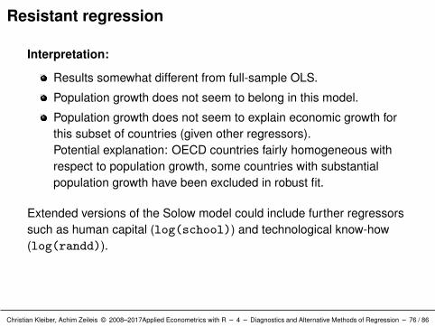
Resistant regression
Interpretation:
Results somewhat different from full-sample OLS.
Population growth does not seem to belong in this model.
Population growth does not seem to explain economic growth forthis subset of countries (given other regressors).Potential explanation: OECD countries fairly homogeneous withrespect to population growth, some countries with substantialpopulation growth have been excluded in robust fit.
Extended versions of the Solow model could include further regressorssuch as human capital (log(school)) and technological know-how(log(randd)).
Christian Kleiber, Achim Zeileis © 2008–2017Applied Econometrics with R – 4 – Diagnostics and Alternative Methods of Regression – 76 / 86
Diagnostics and Alternative Methods of Regression
Quantile Regression
Christian Kleiber, Achim Zeileis © 2008–2017Applied Econometrics with R – 4 – Diagnostics and Alternative Methods of Regression – 77 / 86
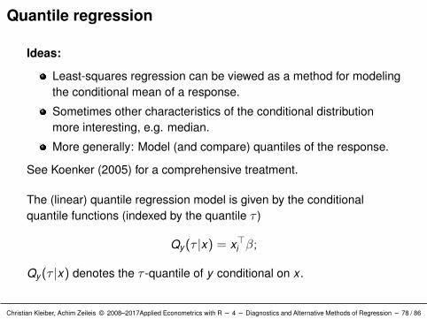
Quantile regression
Ideas:
Least-squares regression can be viewed as a method for modelingthe conditional mean of a response.
Sometimes other characteristics of the conditional distributionmore interesting, e.g. median.
More generally: Model (and compare) quantiles of the response.
See Koenker (2005) for a comprehensive treatment.
The (linear) quantile regression model is given by the conditionalquantile functions (indexed by the quantile τ )
Qy (τ |x) = x>i β;
Qy (τ |x) denotes the τ -quantile of y conditional on x .
Christian Kleiber, Achim Zeileis © 2008–2017Applied Econometrics with R – 4 – Diagnostics and Alternative Methods of Regression – 78 / 86
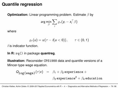
Quantile regression
Optimization: Linear programming problem. Estimate β by
arg minβ
∑i
%τ (yi − x>i β)
where
%τ (u) = uτ − I(u < 0), τ ∈ (0, 1)
I is indicator function.
In R: rq() in package quantreg.
Illustration: Reconsider CPS1988 data and quantile versions of aMincer-type wage equation.
Qlog(wage)(τ |x) = β1 + β2 experience +
β3 experience2 + β4 education
Christian Kleiber, Achim Zeileis © 2008–2017Applied Econometrics with R – 4 – Diagnostics and Alternative Methods of Regression – 79 / 86
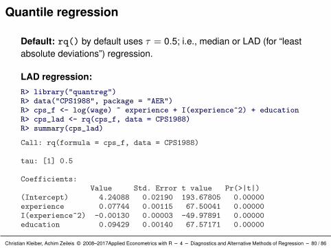
Quantile regression
Default: rq() by default uses τ = 0.5; i.e., median or LAD (for “leastabsolute deviations”) regression.
LAD regression:
R> library("quantreg")R> data("CPS1988", package = "AER")R> cps_f <- log(wage) ~ experience + I(experience^2) + educationR> cps_lad <- rq(cps_f, data = CPS1988)R> summary(cps_lad)
Call: rq(formula = cps_f, data = CPS1988)
tau: [1] 0.5
Coefficients:Value Std. Error t value Pr(>|t|)
(Intercept) 4.24088 0.02190 193.67805 0.00000experience 0.07744 0.00115 67.50041 0.00000I(experience^2) -0.00130 0.00003 -49.97891 0.00000education 0.09429 0.00140 67.57171 0.00000
Christian Kleiber, Achim Zeileis © 2008–2017Applied Econometrics with R – 4 – Diagnostics and Alternative Methods of Regression – 80 / 86
Quantile regression
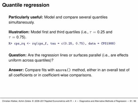
Particularly useful: Model and compare several quantilessimultaneously.
Illustration: Model first and third quartiles (i.e., τ = 0.25 andτ = 0.75).
R> cps_rq <- rq(cps_f, tau = c(0.25, 0.75), data = CPS1988)
Question: Are the regression lines or surfaces parallel (i.e., are effectsuniform across quantiles)?
Answer: Compare fits with anova() method, either in an overall test ofall coefficients or in coefficient-wise comparisons.
Christian Kleiber, Achim Zeileis © 2008–2017Applied Econometrics with R – 4 – Diagnostics and Alternative Methods of Regression – 81 / 86
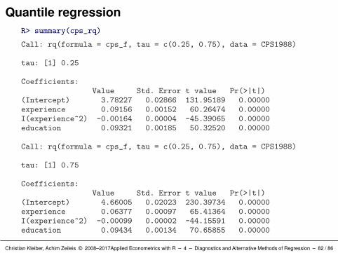
Quantile regressionR> summary(cps_rq)
Call: rq(formula = cps_f, tau = c(0.25, 0.75), data = CPS1988)
tau: [1] 0.25
Coefficients:Value Std. Error t value Pr(>|t|)
(Intercept) 3.78227 0.02866 131.95189 0.00000experience 0.09156 0.00152 60.26474 0.00000I(experience^2) -0.00164 0.00004 -45.39065 0.00000education 0.09321 0.00185 50.32520 0.00000
Call: rq(formula = cps_f, tau = c(0.25, 0.75), data = CPS1988)
tau: [1] 0.75
Coefficients:Value Std. Error t value Pr(>|t|)
(Intercept) 4.66005 0.02023 230.39734 0.00000experience 0.06377 0.00097 65.41364 0.00000I(experience^2) -0.00099 0.00002 -44.15591 0.00000education 0.09434 0.00134 70.65855 0.00000
Christian Kleiber, Achim Zeileis © 2008–2017Applied Econometrics with R – 4 – Diagnostics and Alternative Methods of Regression – 82 / 86
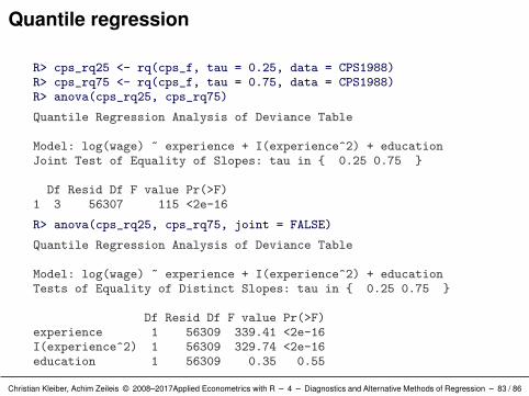
Quantile regression
R> cps_rq25 <- rq(cps_f, tau = 0.25, data = CPS1988)R> cps_rq75 <- rq(cps_f, tau = 0.75, data = CPS1988)R> anova(cps_rq25, cps_rq75)
Quantile Regression Analysis of Deviance Table
Model: log(wage) ~ experience + I(experience^2) + educationJoint Test of Equality of Slopes: tau in 0.25 0.75
Df Resid Df F value Pr(>F)1 3 56307 115 <2e-16
R> anova(cps_rq25, cps_rq75, joint = FALSE)
Quantile Regression Analysis of Deviance Table
Model: log(wage) ~ experience + I(experience^2) + educationTests of Equality of Distinct Slopes: tau in 0.25 0.75
Df Resid Df F value Pr(>F)experience 1 56309 339.41 <2e-16I(experience^2) 1 56309 329.74 <2e-16education 1 56309 0.35 0.55
Christian Kleiber, Achim Zeileis © 2008–2017Applied Econometrics with R – 4 – Diagnostics and Alternative Methods of Regression – 83 / 86
Quantile regression
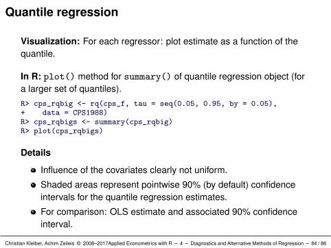
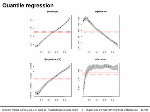
Visualization: For each regressor: plot estimate as a function of thequantile.
In R: plot() method for summary() of quantile regression object (fora larger set of quantiles).R> cps_rqbig <- rq(cps_f, tau = seq(0.05, 0.95, by = 0.05),+ data = CPS1988)R> cps_rqbigs <- summary(cps_rqbig)R> plot(cps_rqbigs)
Details
Influence of the covariates clearly not uniform.
Shaded areas represent pointwise 90% (by default) confidenceintervals for the quantile regression estimates.
For comparison: OLS estimate and associated 90% confidenceinterval.
Christian Kleiber, Achim Zeileis © 2008–2017Applied Econometrics with R – 4 – Diagnostics and Alternative Methods of Regression – 84 / 86
Quantile regression
0.2 0.4 0.6 0.8
3.5
4.0
4.5
5.0
(Intercept)
0.2 0.4 0.6 0.8
0.05
0.06
0.07
0.08
0.09
0.10
experience
0.2 0.4 0.6 0.8
−0.
0020
−0.
0016
−0.
0012
−0.
0008
I(experience^2)
0.2 0.4 0.6 0.8
0.07
0.08
0.09
education
Christian Kleiber, Achim Zeileis © 2008–2017Applied Econometrics with R – 4 – Diagnostics and Alternative Methods of Regression – 85 / 86
Quantile regression
quantreg also contains
Nonlinear and nonparametric quantile modeling functions.
Several algorithms for fitting models (specifically, both exterior andinterior point methods).
Several choices of methods for computing confidence intervalsand related test statistics.
Quantile regression for censored dependent variables (withvarious fitting algorithms).
Christian Kleiber, Achim Zeileis © 2008–2017Applied Econometrics with R – 4 – Diagnostics and Alternative Methods of Regression – 86 / 86