Embed Size (px)
Citation preview
Applied Discrete Structures
Part 2 - Applied Algebra

Applied Discrete StructuresPart 2 - Applied Algebra
Al DoerrUniversity of Massachusetts Lowell
Ken LevasseurUniversity of Massachusetts Lowell
June, 2018
Edition: 3rd Edition - version 5
Website: faculty.uml.edu/klevasseur/ADS2
© 2017 Al Doerr, Ken Levasseur
Applied Discrete Structures by Alan Doerr and Kenneth Levasseur is licensedunder a Creative Commons Attribution-NonCommercial-ShareAlike 3.0 UnitedStates License. You are free to Share: copy and redistribute the material inany medium or format; Adapt: remix, transform, and build upon the material.You may not use the material for commercial purposes. The licensor cannotrevoke these freedoms as long as you follow the license terms.
To our families
Donna, Christopher, Melissa, and Patrick Doerr
Karen, Joseph, Kathryn, and Matthew Levasseur


Acknowledgements
We would like to acknowledge the following instructors for theirhelpful comments and suggestions.
• Tibor Beke, UMass Lowell• Alex DeCourcy, UMass
Lowell• Vince DiChiacchio• Matthew Haner, Mansfield
University (PA)• Dan Klain, UMass Lowell
• Sitansu Mittra, UMassLowell
• Ravi Montenegro, UMassLowell
• Tony Penta, UMass Lowell
• Jim Propp, UMass Lowell
I’d like to particularly single out Jim Propp for his close scrutiny,along with that of his students, who are listed below.
I would like to thank Rob Beezer, David Farmer, Karl-Dieter Crisman andother participants on the pretext-xml-support group for their guidance andwork on MathBook XML, which has now been renamed PreTeXt. Thanks tothe Pedagogy Subcommittee of the UMass Lowell Transformational EducationCommittee for their financial assistance in helping getting this project started.
Many students have provided feedback and pointed out typos inseveral editions of this book. They are listed below. Students withno affiliation listed are from UMass Lowell.
• Ryan Allen• Anju Balaji• Carlos Barrientos• Chris Berns• Raymond Berger, Eckerd
College• Brianne Bindas• Nicholas Bishop• Nathan Blood• Cameron Bolduc• Sam Bouchard• Eric Breslau• Rachel Bryan• Rebecca Campbelli• Eric Carey
• Emily Cashman• Rachel Chaiser, U. ofPuget Sound
• Sam Chambers• Hannah Chiodo• David Connolly• Sean Cummings• Alex DeCourcy• Ryan Delosh• Hillari Denny• Adam Espinola• Josh Everett• Anthony Gaeta• Lisa Gieng• Holly Goodreau• Lilia Heimold
vii

viii
• Kevin Holmes• Alexa Hyde• Michael Ingemi• Kyle Joaquim• Devin Johnson• Jeremy Joubert• William Jozefczyk• Antony Kellermann• Thomas Kiley• Cody Kingman• Leant Seu Kim• Jessica Kramer• John Kuczynski• Justin LaGree• Kendra Lansing• Gregory Lawrence• Pearl Laxague• Kevin Le• Matt LeBlanc• Maxwell Leduc• Ariel Leva• Laura Lucaciu• Andrew Magee• Matthew Malone• Logan Mann• Amy Mazzucotelli• Adam Melle• Jason McAdam• Nick McArdle• Christine McCarthy• Shelbylynn McCoy• Conor McNierney• Albara Mehene• Max Mints• Timothy Miskell
• Mike Morley
• Zach Mulcahy
• Tessa Munoz
• Logan Nadeau
• Carol Nguyen
• Hung Nguyen
• Shelly Noll
• Harsh Patel
• Beck Peterson
• Paola Pevzner
• Samantha Poirier
• Ian Roberts
• John Raisbeck
• Adelia Reid
• Derek Ross
• Jacob Rothmel
• Zach Rush
• Doug Salvati
• Chita Sano
• Ben Shipman
• Florens Shosho
• Jonathan Silva
• Mason Sirois
• Sana Shaikh
• Andrew Somerville
• James Tan
• Bunchhoung Tiv
• Joanel Vasquez
• Anh Vo
• Steve Werren
• Henry Zhu
• Several students atLuzurne County Commu-nity College (PA)
Preface
This is part 2 of Applied Discrete Structures. In order to maintain uniformnumbering and avoid broken links, stubs of the first ten chapters are in-cluded and contain the introduction elements that are referenced in chapters11 through 16. To see all of chapters 1 through 10, visit our web page athttp://faculty.uml.edu/klevasseur/ADS2.
This version of Applied Discrete Structures has been developed using Pre-TeXt, a lightweight XML application for authors of scientific articles, textbooksand monographs initiated by Rob Beezer, U. of Puget Sound.
We embarked on this open-source project in 2010. The choice of Math-ematica for “source code” was based on the speed with which we could dothe conversion. However, the format was not ideal, with no viable web versionavailable. The project has been well-received in spite of these issues. Validationthrough the listing of this project on the American Institute of Mathematicshas been very helpful. When the MBX project was launched, it was the nat-ural next step. The features of MBX make it far more readable than our firstversions, with web, pdf and print copies being far more readable.
Twenty-one years after the publication of the 2nd edition of Applied Dis-crete Structures for Computer Science, in 1989 the publishing and computinglandscape had both changed dramatically. We signed a contract for the secondedition with Science Research Associates in 1988 but by the time the book wasready to print, SRA had been sold to MacMillan. Soon after, the rights hadbeen passed on to Pearson Education, Inc. In 2010, the long-term future ofprinted textbooks is uncertain. In the meantime, textbook prices (both printedand e-books) have increased and a growing open source textbook market move-ment has started. One of our objectives in revisiting this text is to make itavailable to our students in an affordable format. In its original form, the textwas peer-reviewed and was adopted for use at several universities throughoutthe country. For this reason, we see Applied Discrete Structures as not onlyan inexpensive alternative, but a high quality alternative.
As indicated above the computing landscape is very different from the1980’s and accounts for the most significant changes in the text. One of themost common programming languages of the 1980’s was Pascal. We used itto illustrate many of the concepts in the text. Although it isn’t totally dead,Pascal is far from the mainstream of computing in the 21st century. In 1989,Mathematica had been out for less than a year — now a major force in sci-entific computing. The open source software movement also started in thelate 1980’s and in 2005, the first version of Sage, an open-source alternativeto Mathematica, was first released. In Applied Discrete Structures we havereplaced "Pascal Notes" with "Mathematica Notes" and "SageMath Notes."Finally, 1989 was the year that specifications for World Wide Web was laidout by Tim Berners-Lee. There wasn’t a single www in the 2nd edition.
Sage (sagemath.org) is a free, open source, software system for advancedmathematics. Sage can be used either on your own computer, a local server,
ix

x
or on SageMathCloud (https://cloud.sagemath.com).Ken LevasseurLowell MA
Contents
Acknowledgements vii
Preface ix
1 Set Theory I 1
2 Combinatorics 3
3 Logic 5
4 More on Sets 7
5 Introduction to Matrix Algebra 9
6 Relations 11
7 Functions 13Exercises . . . . . . . . . . . . . . . . . . . . . . . . . . . . . . . . . 13
8 Recursion and Recurrence Relations 15
9 Graph Theory 17
10 Trees 19
11 Algebraic Structures 2111.1 Operations . . . . . . . . . . . . . . . . . . . . . . . . . . . . . 2111.2 Algebraic Systems . . . . . . . . . . . . . . . . . . . . . . . . . 2411.3 Some General Properties of Groups . . . . . . . . . . . . . . . . 2911.4 Greatest Common Divisors and the Integers Modulo n . . . . . 3311.5 Subsystems . . . . . . . . . . . . . . . . . . . . . . . . . . . . . 4111.6 Direct Products . . . . . . . . . . . . . . . . . . . . . . . . . . . 4611.7 Isomorphisms . . . . . . . . . . . . . . . . . . . . . . . . . . . . 53
12 More Matrix Algebra 5912.1 Systems of Linear Equations . . . . . . . . . . . . . . . . . . . . 5912.2 Matrix Inversion . . . . . . . . . . . . . . . . . . . . . . . . . . 6812.3 An Introduction to Vector Spaces . . . . . . . . . . . . . . . . . 7112.4 The Diagonalization Process . . . . . . . . . . . . . . . . . . . . 7912.5 Some Applications . . . . . . . . . . . . . . . . . . . . . . . . . 8712.6 Linear Equations over the Integers Mod 2 . . . . . . . . . . . . 93
xi
xii CONTENTS
13 Boolean Algebra 9713.1 Posets Revisited . . . . . . . . . . . . . . . . . . . . . . . . . . 9713.2 Lattices . . . . . . . . . . . . . . . . . . . . . . . . . . . . . . . 10113.3 Boolean Algebras . . . . . . . . . . . . . . . . . . . . . . . . . . 10313.4 Atoms of a Boolean Algebra . . . . . . . . . . . . . . . . . . . . 10713.5 Finite Boolean Algebras as n-tuples of 0’s and 1’s . . . . . . . . 11113.6 Boolean Expressions . . . . . . . . . . . . . . . . . . . . . . . . 112
14 Monoids and Automata 11714.1 Monoids . . . . . . . . . . . . . . . . . . . . . . . . . . . . . . . 11714.2 Free Monoids and Languages . . . . . . . . . . . . . . . . . . . 12014.3 Automata, Finite-State Machines . . . . . . . . . . . . . . . . . 12714.4 The Monoid of a Finite-State Machine . . . . . . . . . . . . . . 13114.5 The Machine of a Monoid . . . . . . . . . . . . . . . . . . . . . 134
15 Group Theory and Applications 13915.1 Cyclic Groups . . . . . . . . . . . . . . . . . . . . . . . . . . . . 13915.2 Cosets and Factor Groups . . . . . . . . . . . . . . . . . . . . . 14515.3 Permutation Groups . . . . . . . . . . . . . . . . . . . . . . . . 15115.4 Normal Subgroups and Group Homomorphisms . . . . . . . . . 16015.5 Coding Theory, Group Codes . . . . . . . . . . . . . . . . . . . 167
16 An Introduction to Rings and Fields 17316.1 Rings, Basic Definitions and Concepts . . . . . . . . . . . . . . 17316.2 Fields . . . . . . . . . . . . . . . . . . . . . . . . . . . . . . . . 18116.3 Polynomial Rings . . . . . . . . . . . . . . . . . . . . . . . . . . 18516.4 Field Extensions . . . . . . . . . . . . . . . . . . . . . . . . . . 19116.5 Power Series . . . . . . . . . . . . . . . . . . . . . . . . . . . . . 195
A Algorithms 201A.1 An Introduction to Algorithms . . . . . . . . . . . . . . . . . . 201A.2 The Invariant Relation Theorem . . . . . . . . . . . . . . . . . 205
B Hints and Solutions to Selected Exercises 209
C Notation 257
References 259
Index 263
Chapter 1
Set Theory I
Goals for Chapter 1This is a stub for Part 2 of Applied Discrete Stuctures. To see the wholechapter, visit our web page at http://faculty.uml.edu/klevasseur/ADS2.
In this chapter we will cover some of the basic set language and notationthat will be used throughout the text. Venn diagrams will be introduced inorder to give the reader a clear picture of set operations. In addition, wewill describe the binary representation of positive integers (Section 1.4) andintroduce summation notation and its generalizations (Section 1.5).
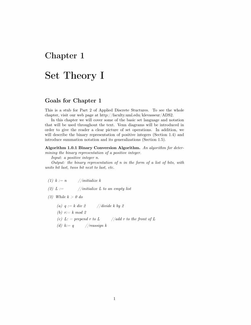
Algorithm 1.0.1 Binary Conversion Algorithm. An algorithm for deter-mining the binary representation of a positive integer.
Input: a positive integer n.Output: the binary representation of n in the form of a list of bits, with
units bit last, twos bit next to last, etc.
(1) k := n //initialize k
(2) L := //initialize L to an empty list
(3) While k > 0 do
(a) q := k div 2 //divide k by 2
(b) r:= k mod 2
(c) L: = prepend r to L //add r to the front of L
(d) k:= q //reassign k
1

2 CHAPTER 1. SET THEORY I
Chapter 2
Combinatorics
This is a stub for Part 2 of Applied Discrete Stuctures. To see the wholechapter, visit our web page at http://faculty.uml.edu/klevasseur/ADS2.
Throughout this book we will be counting things. In this chapter we willoutline some of the tools that will help us count.
Counting occurs not only in highly sophisticated applications of mathemat-ics to engineering and computer science but also in many basic applications.Like many other powerful and useful tools in mathematics, the concepts aresimple; we only have to recognize when and how they can be applied.
3

4 CHAPTER 2. COMBINATORICS
Chapter 3
Logic
This is a stub for Part 2 of Applied Discrete Stuctures. To see the wholechapter, visit our web page at http://faculty.uml.edu/klevasseur/ADS2.
In this chapter, we will introduce some of the basic concepts of mathemat-ical logic. In order to fully understand some of the later concepts in this book,you must be able to recognize valid logical arguments. Although these argu-ments will usually be applied to mathematics, they employ the same techniquesthat are used by a lawyer in a courtroom or a physician examining a patient.An added reason for the importance of this chapter is that the circuits thatmake up digital computers are designed using the same algebra of propositionsthat we will be discussing.
5

6 CHAPTER 3. LOGIC
Chapter 4
More on Sets
This is a stub for Part 2 of Applied Discrete Stuctures. To see the wholechapter, visit our web page at http://faculty.uml.edu/klevasseur/ADS2.
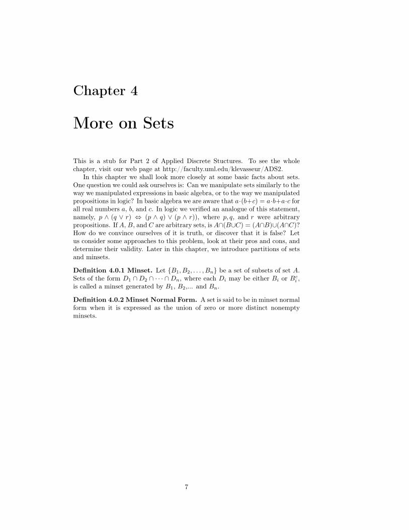
In this chapter we shall look more closely at some basic facts about sets.One question we could ask ourselves is: Can we manipulate sets similarly to theway we manipulated expressions in basic algebra, or to the way we manipulatedpropositions in logic? In basic algebra we are aware that a·(b+c) = a·b+a·c forall real numbers a, b, and c. In logic we verified an analogue of this statement,namely, p ∧ (q ∨ r) ⇔ (p ∧ q) ∨ (p ∧ r)), where p, q, and r were arbitrarypropositions. IfA, B, and C are arbitrary sets, isA∩(B∪C) = (A∩B)∪(A∩C)?How do we convince ourselves of it is truth, or discover that it is false? Letus consider some approaches to this problem, look at their pros and cons, anddetermine their validity. Later in this chapter, we introduce partitions of setsand minsets.
Definition 4.0.1 Minset. Let {B1, B2, . . . , Bn} be a set of subsets of set A.Sets of the form D1 ∩D2 ∩ · · · ∩Dn, where each Di may be either Bi or Bci ,is called a minset generated by B1, B2,... and Bn.
Definition 4.0.2 Minset Normal Form. A set is said to be in minset normalform when it is expressed as the union of zero or more distinct nonemptyminsets.
7

8 CHAPTER 4. MORE ON SETS
Chapter 5
Introduction to MatrixAlgebra
This is a stub for Part 2 of Applied Discrete Stuctures. To see the wholechapter, visit our web page at http://faculty.uml.edu/klevasseur/ADS2.
The purpose of this chapter is to introduce you to matrix algebra, which hasmany applications. You are already familiar with several algebras: elementaryalgebra, the algebra of logic, the algebra of sets. We hope that as you studiedthe algebra of logic and the algebra of sets, you compared them with elementaryalgebra and noted that the basic laws of each are similar. We will see thatmatrix algebra is also similar. As in previous discussions, we begin by definingthe objects in question and the basic operations.
9

10 CHAPTER 5. INTRODUCTION TO MATRIX ALGEBRA
Chapter 6
Relations
This is a stub for Part 2 of Applied Discrete Stuctures. To see the wholechapter, visit our web page at http://faculty.uml.edu/klevasseur/ADS2.
One understands a set of objects completely only if the structure of thatset is made clear by the interrelationships between its elements. For example,the individuals in a crowd can be compared by height, by age, or throughany number of other criteria. In mathematics, such comparisons are calledrelations. The goal of this chapter is to develop the language, tools, andconcepts of relations.
11
12 CHAPTER 6. RELATIONS
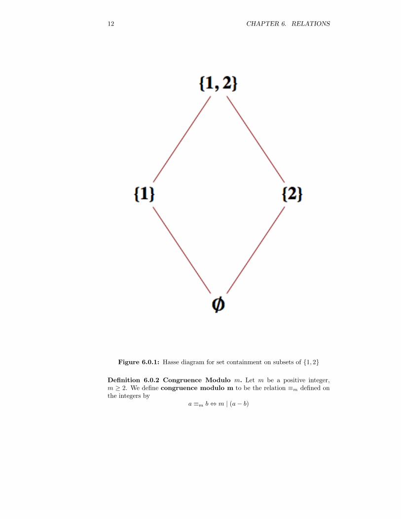
Figure 6.0.1: Hasse diagram for set containment on subsets of {1, 2}
Definition 6.0.2 Congruence Modulo m. Let m be a positive integer,m ≥ 2. We define congruence modulo m to be the relation ≡m defined onthe integers by
a ≡m b⇔ m | (a− b)
Chapter 7
Functions
This is a stub for Part 2 of Applied Discrete Stuctures. To see the wholechapter, visit our web page at http://faculty.uml.edu/klevasseur/ADS2.
In this chapter we will consider some basic concepts of the relations that arecalled functions. A large variety of mathematical ideas and applications canbe more completely understood when expressed through the function concept.
Theorem 7.0.1 The composition of injections is an injection. If f :A→ B and g : B → C are injections, then g ◦ f : A→ C is an injection.
Theorem 7.0.2 The composition of surjections is a surjection. If f :A→ B and g : B → C are surjections, then g ◦ f : A→ C is a surjection.
Exercises7. If A and B are finite sets, how many different functions are there from Ainto B?
13

14 CHAPTER 7. FUNCTIONS
Chapter 8
Recursion and RecurrenceRelations
This is a stub for Part 2 of Applied Discrete Stuctures. To see the wholechapter, visit our web page at http://faculty.uml.edu/klevasseur/ADS2.
An essential tool that anyone interested in computer science must masteris how to think recursively. The ability to understand definitions, concepts,algorithms, etc., that are presented recursively and the ability to put thoughtsinto a recursive framework are essential in computer science. One of our goalsin this chapter is to help the reader become more comfortable with recursionin its commonly encountered forms.
A second goal is to discuss recurrence relations. We will concentrate onmethods of solving recurrence relations, including an introduction to generatingfunctions.
Algorithm 8.0.1 Algorithm for Solving Homogeneous Finite-orderLinear Relations.
(a) Write out the characteristic equation of the relation S(k) +C1S(k− 1) +. . .+ CnS(k − n) = 0, which is an + C1a
n−1 + · · ·+ Cn−1a+ Cn = 0.
(b) Find all roots of the characteristic equation, the characteristic roots.
(c) If there are n distinct characteristic roots, a1, a2, . . . an, then the generalsolution of the recurrence relation is S(k) = b1a1
k + b2a2k + · · ·+ bnan
k.If there are fewer than n characteristic roots, then at least one root is amultiple root. If aj is a double root, then the bjajk term is replaced with(bj0 + bj1k) akj . In general, if aj is a root of multiplicity p, then the bjajk
term is replaced with(bj0 + bj1k + · · ·+ bj(p−1)k
p−1)akj .
(d) If n initial conditions are given, we get n linear equations in n unknowns(the bj ′s from Step 3) by substitution. If possible, solve these equationsto determine a final form for S(k).
Example 8.0.2 Solution of a Third Order Recurrence Relation. SolveS(k)− 7S(k − 2) + 6S(k − 3) = 0, where S(0) = 8, S(1) = 6, and S(2) = 22.
(a) The characteristic equation is a3 − 7a+ 6 = 0.
(b) The only rational roots that we can attempt are ±1,±2,±3, and± 6. Bychecking these, we obtain the three roots 1, 2, and −3.
15
16 CHAPTER 8. RECURSION AND RECURRENCE RELATIONS
(c) The general solution is S(k) = b11k + b22k + b3(−3)k. The first term cansimply be written b1 .
(d)
S(0) = 8
S(1) = 6
S(2) = 22
⇒
b1 + b2 + b3 = 8
b1 + 2b2 − 3b3 = 6
b1 + 4b2 + 9b3 = 22
You can solve this sys-
tem by elimination to obtain b1 = 5, b2 = 2, and b3 = 1. Therefore,S(k) = 5 + 2 · 2k + (−3)k = 5 + 2k+1 + (−3)k
Chapter 9
Graph Theory
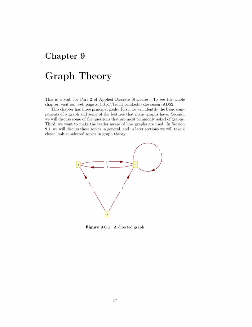
This is a stub for Part 2 of Applied Discrete Stuctures. To see the wholechapter, visit our web page at http://faculty.uml.edu/klevasseur/ADS2.
This chapter has three principal goals. First, we will identify the basic com-ponents of a graph and some of the features that many graphs have. Second,we will discuss some of the questions that are most commonly asked of graphs.Third, we want to make the reader aware of how graphs are used. In Section9.1, we will discuss these topics in general, and in later sections we will take acloser look at selected topics in graph theory.
Figure 9.0.1: A directed graph
17

18 CHAPTER 9. GRAPH THEORY
Chapter 10
Trees
This is a stub for Part 2 of Applied Discrete Stuctures. To see the wholechapter, visit our web page at http://faculty.uml.edu/klevasseur/ADS2.
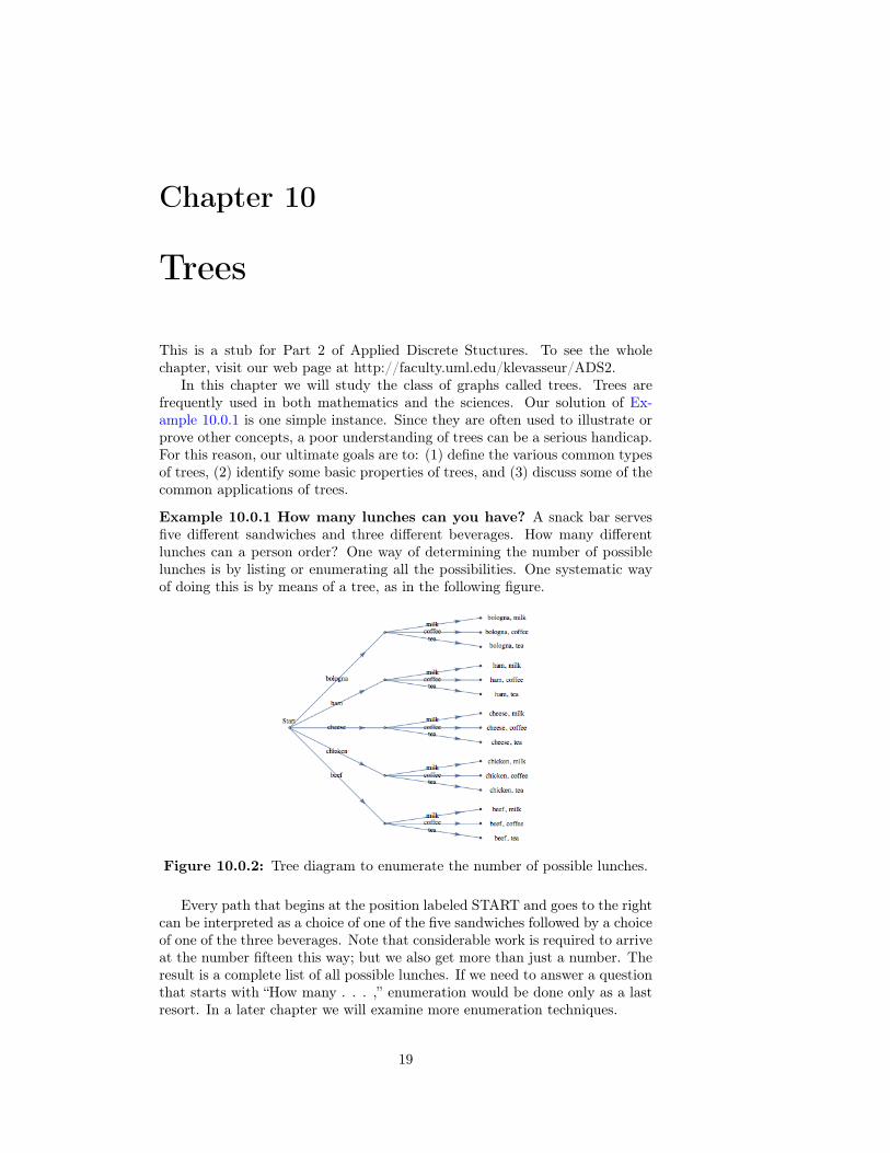
In this chapter we will study the class of graphs called trees. Trees arefrequently used in both mathematics and the sciences. Our solution of Ex-ample 10.0.1 is one simple instance. Since they are often used to illustrate orprove other concepts, a poor understanding of trees can be a serious handicap.For this reason, our ultimate goals are to: (1) define the various common typesof trees, (2) identify some basic properties of trees, and (3) discuss some of thecommon applications of trees.
Example 10.0.1 How many lunches can you have? A snack bar servesfive different sandwiches and three different beverages. How many differentlunches can a person order? One way of determining the number of possiblelunches is by listing or enumerating all the possibilities. One systematic wayof doing this is by means of a tree, as in the following figure.
Figure 10.0.2: Tree diagram to enumerate the number of possible lunches.
Every path that begins at the position labeled START and goes to the rightcan be interpreted as a choice of one of the five sandwiches followed by a choiceof one of the three beverages. Note that considerable work is required to arriveat the number fifteen this way; but we also get more than just a number. Theresult is a complete list of all possible lunches. If we need to answer a questionthat starts with “How many . . . ,” enumeration would be done only as a lastresort. In a later chapter we will examine more enumeration techniques.
19

20 CHAPTER 10. TREES
Chapter 11
Algebraic Structures
The primary goal of this chapter is to make the reader aware of what an alge-braic system is and how algebraic systems can be studied at different levels ofabstraction. After describing the concrete, axiomatic, and universal levels, wewill introduce one of the most important algebraic systems at the axiomaticlevel, the group. In this chapter, group theory will be a vehicle for introducingthe universal concepts of isomorphism, direct product, subsystem, and generat-ing set. These concepts can be applied to all algebraic systems. The simplicityof group theory will help the reader obtain a good intuitive understanding ofthese concepts. In Chapter 15, we will introduce some additional concepts andapplications of group theory. We will close the chapter with a discussion of howsome computer hardware and software systems use the concept of an algebraicsystem.
11.1 OperationsOne of the first mathematical skills that we all learn is how to add a pair ofpositive integers. A young child soon recognizes that something is wrong if asum has two values, particularly if his or her sum is different from the teacher’s.In addition, it is unlikely that a child would consider assigning a non-positivevalue to the sum of two positive integers. In other words, at an early age weprobably know that the sum of two positive integers is unique and belongs tothe set of positive integers. This is what characterizes all binary operations ona set.
11.1.1 What is an Operation?Definition 11.1.1 Binary Operation. Let S be a nonempty set. A binaryoperation on S is a rule that assigns to each ordered pair of elements of S aunique element of S. In other words, a binary operation is a function fromS × S into S.
Example 11.1.2 Some common binary operations. Union and intersec-tion are both binary operations on the power set of any universe. Addition andmultiplication are binary operators on the natural numbers. Addition and mul-tiplication are binary operations on the set of 2 by 2 real matrices, M2×2(R).Division is a binary operation on some sets of numbers, such as the positivereals. But on the integers (1/2 /∈ Z) and even on the real numbers (1/0 is notdefined), division is not a binary operation.
Note 11.1.3.
21
22 CHAPTER 11. ALGEBRAIC STRUCTURES
(a) We stress that the image of each ordered pair must be in S. This require-ment disqualifies subtraction on the natural numbers from considerationas a binary operation, since 1 − 2 is not a natural number. Subtractionis a binary operation on the integers.
(b) On Notation. Despite the fact that a binary operation is a function,symbols, not letters, are used to name them. The most commonly usedsymbol for a binary operation is an asterisk, ∗. We will also use a dia-mond, �, when a second symbol is needed.
If ∗ is a binary operation on S and a, b ∈ S, there are three common waysof denoting the image of the pair (a, b). They are:
∗ab a ∗ b ab∗Prefix Form Infix Form Postfix Form
We are all familiar with infix form. For example, 2+3 is how everyone is taughtto write the sum of 2 and 3. But notice how 2 + 3 was just described in theprevious sentence! The word sum preceded 2 and 3. Orally, prefix form is quitenatural to us. The prefix and postfix forms are superior to infix form in somerespects. In Chapter 10, we saw that algebraic expressions with more thanone operation didn’t need parentheses if they were in prefix or postfix form.However, due to our familiarity with infix form, we will use it throughout mostof the remainder of this book.
Some operations, such as negation of numbers and complementation of sets,are not binary, but unary operators.
Definition 11.1.4 Unary Operation. Let S be a nonempty set. A unaryoperator on S is a rule that assigns to each element of S a unique element ofS. In other words, a unary operator is a function from S into S.
11.1.2 Properties of Operations
Whenever an operation on a set is encountered, there are several properties thatshould immediately come to mind. To effectively make use of an operation, youshould know which of these properties it has. By now, you should be familiarwith most of these properties. We will list the most common ones here torefresh your memory and define them for the first time in a general setting.
First we list properties of a single binary operation.
Definition 11.1.5 Commutative Property. Let ∗ be a binary operationon a set S. We say that * is commutative if and only if a ∗ b = b ∗ a for alla, b ∈ S.
Definition 11.1.6 Associative Property. Let ∗ be a binary operation on aset S. We say that ∗ is associative if and only if (a ∗ b) ∗ c = a ∗ (b ∗ c) for alla, b, c ∈ S.
Definition 11.1.7 Identity Property. Let ∗ be a binary operation on a setS. We say that ∗ has an identity if and only if there exists an element, e, inS such that a ∗ e = e ∗ a = a for all a ∈ S.
The next property presumes that ∗ has the identity property.
Definition 11.1.8 Inverse Property. Let ∗ be a binary operation on a setS. We say that ∗ has the inverse property if and only if for each a ∈ S,there exists b ∈ S such that a ∗ b = b ∗ a = e. We call b an inverse of a.
11.1. OPERATIONS 23
Definition 11.1.9 Idempotent Property. Let ∗ be a binary operation ona set S. We say that ∗ is idempotent if and only if a ∗ a = a for all a ∈ S.
Now we list properties that apply to two binary operations.
Definition 11.1.10 Left Distributive Property. Let ∗ and � be binaryoperations on a set S. We say that � is left distributive over * if and only ifa � (b ∗ c) = (a � b) ∗ (a � c) for all a, b, c ∈ S.
Definition 11.1.11 Right Distributive Property. Let ∗ and � be binaryoperations on a set S. We say that � is right distributive over * if and only if(b ∗ c) � a = (b � a) ∗ (c � a) for all a, b, c ∈ S.
Definition 11.1.12 Distributive Property. Let ∗ and � be binary opera-tions on a set S. We say that � is distributive over ∗ if and only if � is bothleft and right distributive over ∗.
There is one significant property of unary operations.
Definition 11.1.13 Involution Property. Let − be a unary operation onS. We say that − has the involution property if −(−a) = a for all a ∈ S.
Finally, a property of sets, as they relate to operations.
Definition 11.1.14 Closure Property. Let T be a subset of S and let ∗ bea binary operation on S. We say that T is closed under ∗ if a, b ∈ T impliesthat a ∗ b ∈ T .
In other words, T is closed under ∗ if by operating on elements of T with∗, you can’t get new elements that are outside of T .
Example 11.1.15 Some examples of closure and non-closure.
(a) The odd integers are closed under multiplication, but not under addition.
(b) Let p be a proposition over U and let A be the set of propositions overU that imply p. That is; q ∈ A if q ⇒ p. Then A is closed under bothconjunction and disjunction.
(c) The set of positive integers that are multiples of 5 is closed under bothaddition and multiplication.
It is important to realize that the properties listed above depend on both theset and the operation(s). Statements such as “Multiplication is commutative.”or “The positive integers are closed.” are meaningless on their own. Naturally,if we have established a context in which the missing set or operation is clearlyimplied, then they would have meaning.
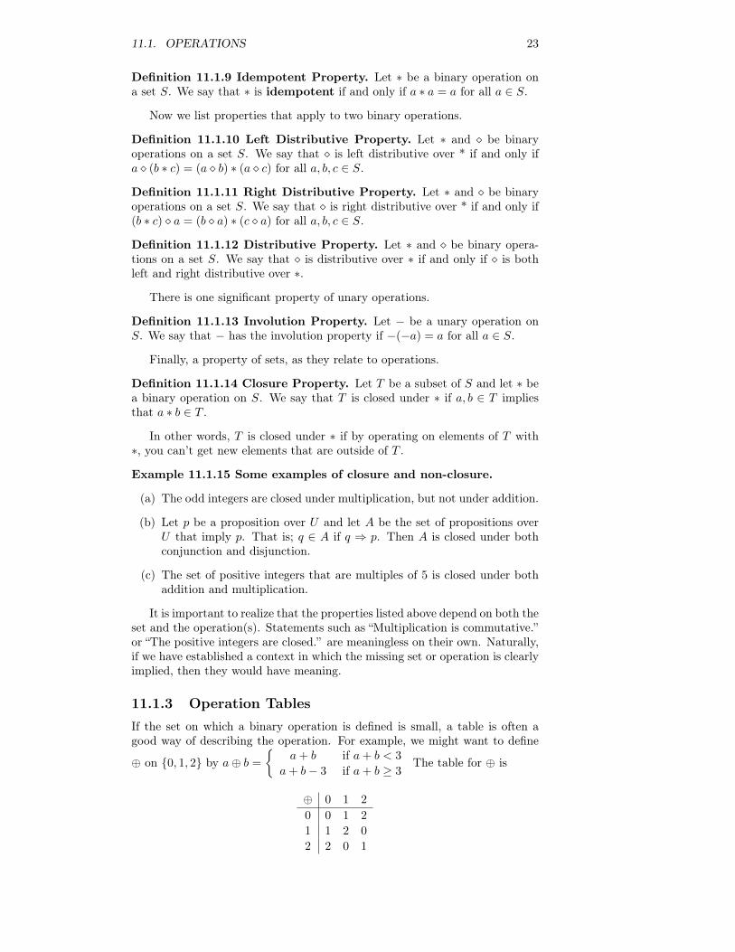
11.1.3 Operation TablesIf the set on which a binary operation is defined is small, a table is often agood way of describing the operation. For example, we might want to define
⊕ on {0, 1, 2} by a⊕ b =
{a+ b if a+ b < 3
a+ b− 3 if a+ b ≥ 3The table for ⊕ is
⊕ 0 1 2
0 0 1 2
1 1 2 0
2 2 0 1
24 CHAPTER 11. ALGEBRAIC STRUCTURES
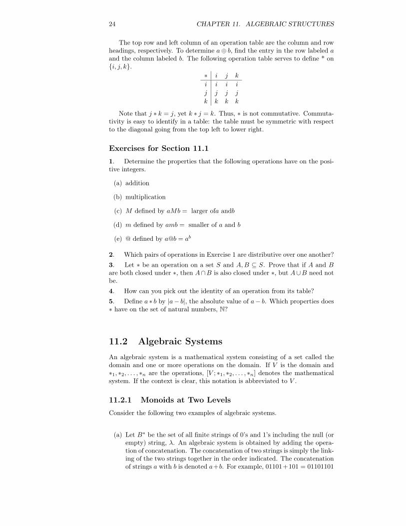
The top row and left column of an operation table are the column and rowheadings, respectively. To determine a⊕ b, find the entry in the row labeled aand the column labeled b. The following operation table serves to define * on{i, j, k}.
∗ i j k
i i i i
j j j j
k k k k
Note that j ∗ k = j, yet k ∗ j = k. Thus, ∗ is not commutative. Commuta-tivity is easy to identify in a table: the table must be symmetric with respectto the diagonal going from the top left to lower right.
Exercises for Section 11.1
1. Determine the properties that the following operations have on the posi-tive integers.
(a) addition
(b) multiplication
(c) M defined by aMb = larger ofa andb
(d) m defined by amb = smaller of a and b
(e) @ defined by a@b = ab
2. Which pairs of operations in Exercise 1 are distributive over one another?3. Let ∗ be an operation on a set S and A,B ⊆ S. Prove that if A and Bare both closed under ∗, then A∩B is also closed under ∗, but A∪B need notbe.4. How can you pick out the identity of an operation from its table?5. Define a ∗ b by |a− b|, the absolute value of a− b. Which properties does∗ have on the set of natural numbers, N?
11.2 Algebraic Systems
An algebraic system is a mathematical system consisting of a set called thedomain and one or more operations on the domain. If V is the domain and∗1, ∗2, . . . , ∗n are the operations, [V ; ∗1, ∗2, . . . , ∗n] denotes the mathematicalsystem. If the context is clear, this notation is abbreviated to V .
11.2.1 Monoids at Two Levels
Consider the following two examples of algebraic systems.
(a) Let B∗ be the set of all finite strings of 0’s and 1’s including the null (orempty) string, λ. An algebraic system is obtained by adding the opera-tion of concatenation. The concatenation of two strings is simply the link-ing of the two strings together in the order indicated. The concatenationof strings a with b is denoted a+b. For example, 01101+101 = 01101101
11.2. ALGEBRAIC SYSTEMS 25
and λ+ 100 = 100. Note that concatenation is an associative operationand that λ is the identity for concatenation.A note on notation: There isn’t a standard symbol for concatenation.We have chosen + to be consistent with the notation used in Python andSage for the concatenation.
(b) Let M be any nonempty set and let * be any operation on M that isassociative and has an identity in M .
Our second example might seem strange, but we include it to illustrate apoint. The algebraic system [B∗; +] is a special case of [M ; ∗]. Most of usare much more comfortable with B∗ than with M . No doubt, the reason isthat the elements in B∗ are more concrete. We know what they look like andexactly how they are combined. The description of M is so vague that wedon’t even know what the elements are, much less how they are combined.Why would anyone want to study M? The reason is related to this question:What theorems are of interest in an algebraic system? Answering this questionis one of our main objectives in this chapter. Certain properties of algebraicsystems are called algebraic properties, and any theorem that says somethingabout the algebraic properties of a system would be of interest. The ability toidentify what is algebraic and what isn’t is one of the skills that you shouldlearn from this chapter.
Now, back to the question of why we study M . Our answer is to illustratethe usefulness of M with a theorem about M .
Theorem 11.2.1 A Monoid Theorem. If a, b are elements ofM and a∗b =b ∗ a, then (a ∗ b) ∗ (a ∗ b) = (a ∗ a) ∗ (b ∗ b).
Proof.
(a ∗ b) ∗ (a ∗ b) = a ∗ (b ∗ (a ∗ b)) Why?= a ∗ ((b ∗ a) ∗ b) Why?= a ∗ ((a ∗ b) ∗ b) Why?= a ∗ (a ∗ (b ∗ b)) Why?= (a ∗ a) ∗ (b ∗ b) Why?
The power of this theorem is that it can be applied to any algebraic systemthat M describes. Since B∗ is one such system, we can apply Theorem 11.2.1to any two strings that commute. For example, 01 and 0101. Although aspecial case of this theorem could have been proven for B∗, it would not havebeen any easier to prove, and it would not have given us any insight into otherspecial cases of M .
Example 11.2.2 Another Monoid. Consider the set of 2 × 2 real ma-trices, M2×2(R), with the operation of matrix multiplication. In this con-text, Theorem 11.2.1 can be interpreted as saying that if AB = BA, then
(AB)2 = A2B2. One pair of matrices that this theorem applies to is(
2 1
1 2
)and
(3 −4
−4 3
).
11.2.2 Levels of AbstractionOne of the fundamental tools in mathematics is abstraction. There are threelevels of abstraction that we will identify for algebraic systems: concrete, ax-iomatic, and universal.
26 CHAPTER 11. ALGEBRAIC STRUCTURES
11.2.2.1 The Concrete Level
Almost all of the mathematics that you have done in the past was at theconcrete level. As a rule, if you can give examples of a few typical elements ofthe domain and describe how the operations act on them, you are describinga concrete algebraic system. Two examples of concrete systems are B∗ andM2×2(R). A few others are:
(a) The integers with addition. Of course, addition isn’t the only standardoperation that we could include. Technically, if we were to add multipli-cation, we would have a different system.
(b) The subsets of the natural numbers, with union, intersection, and com-plementation.
(c) The complex numbers with addition and multiplication.
11.2.2.2 The Axiomatic Level
The next level of abstraction is the axiomatic level. At this level, the elementsof the domain are not specified, but certain axioms are stated about the numberof operations and their properties. The system that we calledM is an axiomaticsystem. Some combinations of axioms are so common that a name is given toany algebraic system to which they apply. Any system with the propertiesof M is called a monoid. The study of M would be called monoid theory.The assumptions that we made about M , associativity and the existence ofan identity, are called the monoid axioms. One of your few brushes withthe axiomatic level may have been in your elementary algebra course. Manyalgebra texts identify the properties of the real numbers with addition andmultiplication as the field axioms. As we will see in Chapter 16, “Rings andFields,” the real numbers share these axioms with other concrete systems, allof which are called fields.
11.2.2.3 The Universal Level
The final level of abstraction is the universal level. There are certain concepts,called universal algebra concepts, that can be applied to the study of all al-gebraic systems. Although a purely universal approach to algebra would bemuch too abstract for our purposes, defining concepts at this level should makeit easier to organize the various algebraic theories in your own mind. In thischapter, we will consider the concepts of isomorphism, subsystem, and directproduct.
11.2.3 Groups
To illustrate the axiomatic level and the universal concepts, we will consideryet another kind of axiomatic system, the group. In Chapter 5 we noted thatthe simplest equation in matrix algebra that we are often called upon to solveis AX = B, where A and B are known square matrices and X is an unknownmatrix. To solve this equation, we need the associative, identity, and inverselaws. We call the systems that have these properties groups.
Definition 11.2.3 Group. A group consists of a nonempty setG and a binaryoperation ∗ on G satisfying the properties
(a) ∗ is associative on G: (a ∗ b) ∗ c = a ∗ (b ∗ c) for all a, b, c ∈ G.
11.2. ALGEBRAIC SYSTEMS 27
(b) There exists an identity element, e ∈ G such that a ∗ e = e ∗ a = a for alla ∈ G.
(c) For all a ∈ G, there exists an inverse, there exist b ∈ G such that a ∗ b =b ∗ a = e.
A group is usually denoted by its set’s name, G, or occasionally by [G; ∗]to emphasize the operation. At the concrete level, most sets have a standardoperation associated with them that will form a group. As we will see below,the integers with addition is a group. Therefore, in group theory Z alwaysstands for [Z; +].
Note 11.2.4 Generic Symbols. At the axiomatic and universal levels, thereare often symbols that have a special meaning attached to them. In grouptheory, the letter e is used to denote the identity element of whatever groupis being discussed. A little later, we will prove that the inverse of a groupelement, a, is unique and its inverse is usually denoted a−1 and is read “ainverse.” When a concrete group is discussed, these symbols are dropped infavor of concrete symbols. These concrete symbols may or may not be similarto the generic symbols. For example, the identity element of the group ofintegers is 0, and the inverse of n is denoted by −n, the additive inverse of n.
The asterisk could also be considered a generic symbol since it is used todenote operations on the axiomatic level.
Example 11.2.5 Some concrete groups.
(a) The integers with addition is a group. We know that addition is associa-tive. Zero is the identity for addition: 0 + n = n+ 0 = n for all integersn. The additive inverse of any integer is obtained by negating it. Thusthe inverse of n is −n.
(b) The integers with multiplication is not a group. Although multiplicationis associative and 1 is the identity for multiplication, not all integers havea multiplicative inverse in Z. For example, the multiplicative inverse of10 is 1
10 , but110 is not an integer.
(c) The power set of any set U with the operation of symmetric difference,⊕, is a group. If A and B are sets, then A⊕B = (A∪B)− (A∩B). Wewill leave it to the reader to prove that ⊕ is associative over P(U). Theidentity of the group is the empty set: A ⊕ ∅ = A. Every set is its owninverse since A ⊕ A = ∅. Note that P(U) is not a group with union orintersection.
Definition 11.2.6 Abelian Group. A group is abelian if its operation iscommutative.
Abel Most of the groups that we will discuss in this book will beabelian. The term abelian is used to honor the Norwegian mathemati-cian N. Abel (1802-29), who helped develop group theory.
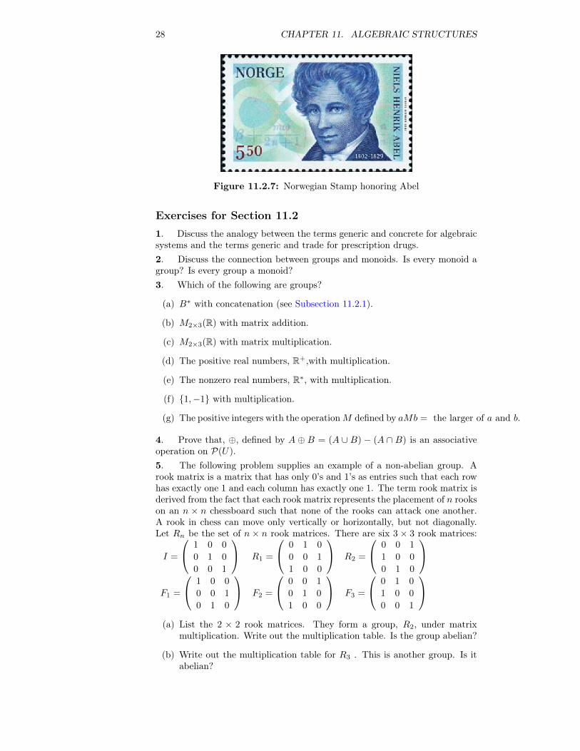
28 CHAPTER 11. ALGEBRAIC STRUCTURES
Figure 11.2.7: Norwegian Stamp honoring Abel
Exercises for Section 11.21. Discuss the analogy between the terms generic and concrete for algebraicsystems and the terms generic and trade for prescription drugs.2. Discuss the connection between groups and monoids. Is every monoid agroup? Is every group a monoid?3. Which of the following are groups?
(a) B∗ with concatenation (see Subsection 11.2.1).
(b) M2×3(R) with matrix addition.
(c) M2×3(R) with matrix multiplication.
(d) The positive real numbers, R+,with multiplication.
(e) The nonzero real numbers, R∗, with multiplication.
(f) {1,−1} with multiplication.
(g) The positive integers with the operationM defined by aMb = the larger of a and b.
4. Prove that, ⊕, defined by A ⊕ B = (A ∪ B) − (A ∩ B) is an associativeoperation on P(U).5. The following problem supplies an example of a non-abelian group. Arook matrix is a matrix that has only 0’s and 1’s as entries such that each rowhas exactly one 1 and each column has exactly one 1. The term rook matrix isderived from the fact that each rook matrix represents the placement of n rookson an n × n chessboard such that none of the rooks can attack one another.A rook in chess can move only vertically or horizontally, but not diagonally.Let Rn be the set of n × n rook matrices. There are six 3 × 3 rook matrices:
I =
1 0 0
0 1 0
0 0 1
R1 =
0 1 0
0 0 1
1 0 0
R2 =
0 0 1
1 0 0
0 1 0
F1 =
1 0 0
0 0 1
0 1 0
F2 =
0 0 1
0 1 0
1 0 0
F3 =
0 1 0
1 0 0
0 0 1
(a) List the 2 × 2 rook matrices. They form a group, R2, under matrix
multiplication. Write out the multiplication table. Is the group abelian?
(b) Write out the multiplication table for R3 . This is another group. Is itabelian?
11.3. SOME GENERAL PROPERTIES OF GROUPS 29
(c) How many 4×4 rook matrices are there? How many n×n rook matricesare there?
6. For each of the following sets, identify the standard operation that resultsin a group. What is the identity of each group?
(a) The set of all 2× 2 matrices with real entries and nonzero determinants.
(b) The set of 2× 3 matrices with rational entries.
7. Let V = {e, a, b, c}. Let ∗ be defined (partially) by x∗x = e for all x ∈ V .Write a complete table for ∗ so that [V ; ∗] is a group.
11.3 Some General Properties of GroupsIn this section, we will present some of the most basic theorems of grouptheory. Keep in mind that each of these theorems tells us something aboutevery group. We will illustrate this point with concrete examples at the closeof the section.
11.3.1 First TheoremsTheorem 11.3.1 Identities are Unique. The identity of a group is unique.
One difficulty that students often encounter is how to get started in provinga theorem like this. The difficulty is certainly not in the theorem’s complexity.It’s too terse! Before actually starting the proof, we rephrase the theorem sothat the implication it states is clear.
Theorem 11.3.2 Identities are Unique - Rephrased. If G = [G; ∗] is agroup and e is an identity of G, then no other element of G is an identity ofG.
Proof. (Indirect): Suppose that f ∈ G, f 6= e, and f is an identity of G. Wewill show that f = e, which is a contradiction, completing the proof.
f = f ∗ e Since e is an identity= e Since f is an identity
Next we justify the phrase “... the inverse of an element of a group.”
Theorem 11.3.3 Inverses are Unique. The inverse of any element of agroup is unique.
The same problem is encountered here as in the previous theorem. We willleave it to the reader to rephrase this theorem. The proof is also left to thereader to write out in detail. Here is a hint: If b and c are both inverses of a,then you can prove that b = c. If you have difficulty with this proof, note thatwe have already proven it in a concrete setting in Chapter 5.
As mentioned above, the significance of Theorem 11.3.3 is that we can referto the inverse of an element without ambiguity. The notation for the inverseof a is usually a−1 (note the exception below).
Example 11.3.4 Some Inverses.
(a) In any group, e−1 is the inverse of the identity e, which always is e.
30 CHAPTER 11. ALGEBRAIC STRUCTURES
(b)(a−1
)−1 is the inverse of a−1 , which is always equal to a (see Theo-rem 11.3.5 below).
(c) (x ∗ y ∗ z)−1 is the inverse of x ∗ y ∗ z.
(d) In a concrete group with an operation that is based on addition, theinverse of a is usually written −a. For example, the inverse of k − 3 inthe group [Z; +] is written −(k−3) = 3−k. In the group of 2×2 matrices
over the real numbers under matrix addition, the inverse of(
4 1
1 −3
)is written −
(4 1
1 −3
), which equals
(−4 −1
−1 3
).
Theorem 11.3.5 Inverse of Inverse Theorem. If a is an element of groupG, then
(a−1
)−1= a.
Again, we rephrase the theorem to make it clear how to proceed.
Theorem 11.3.6 Inverse of Inverse Theorem (Rephrased). If a hasinverse b and b has inverse c, then a = c.
Proof.
a = a ∗ e e is the identity of G= a ∗ (b ∗ c) because c is the inverse of b= (a ∗ b) ∗ c why?= e ∗ c why?= c by the identity property
The next theorem gives us a formula for the inverse of a ∗ b. This formulashould be familiar. In Chapter 5 we saw that if A and B are invertible matrices,then (AB)−1 = B−1A−1.
Theorem 11.3.7 Inverse of a Product. If a and b are elements of groupG, then (a ∗ b)−1 = b−1 ∗ a−1.
Proof. Let x = b−1 ∗ a−1. We will prove that x inverts a ∗ b. Since we knowthat the inverse is unique, we will have proved the theorem.
(a ∗ b) ∗ x = (a ∗ b) ∗(b−1 ∗ a−1
)= a ∗
(b ∗(b−1 ∗ a−1
))= a ∗
((b ∗ b−1
)∗ a−1
)= a ∗
(e ∗ a−1
)= a ∗ a−1
= e
Similarly, x ∗ (a ∗ b) = e; therefore, (a ∗ b)−1 = x = b−1 ∗ a−1
Theorem 11.3.8 Cancellation Laws. If a, b, and c are elements of groupG, then
left cancellation: (a ∗ b = a ∗ c)⇒ b = c
right cancellation: (b ∗ a = c ∗ a)⇒ b = c
11.3. SOME GENERAL PROPERTIES OF GROUPS 31
Proof. We will prove the left cancellation law. The right law can be provedin exactly the same way. Starting with a ∗ b = a ∗ c, we can operate on botha ∗ b and a ∗ c on the left with a−1:
a−1 ∗ (a ∗ b) = a−1 ∗ (a ∗ c)
Applying the associative property to both sides we get
(a−1 ∗ a) ∗ b = (a−1 ∗ a) ∗ c⇒ e ∗ b = e ∗ c⇒ b = c
Theorem 11.3.9 Linear Equations in a Group. If G is a group and a, b ∈G, the equation a ∗ x = b has a unique solution, x = a−1 ∗ b. In addition, theequation x ∗ a = b has a unique solution, x = b ∗ a−1.
Proof. We prove the theorem only for a ∗ x = b, since the second statementis proven identically.
a ∗ x = b = e ∗ b= (a ∗ a−1) ∗ b= a ∗ (a−1 ∗ b)
By the cancellation law, we can conclude that x = a−1 ∗ b.If c and d are two solutions of the equation a ∗ x = b, then a ∗ c = b = a ∗ d
and, by the cancellation law, c = d. This verifies that a−1 ∗ b is the onlysolution of a ∗ x = b.
Note 11.3.10. Our proof of Theorem 11.3.9 was analogous to solving theconcrete equation 4x = 9 in the following way:
4x = 9 =
(4 · 1
4
)9 = 4
(1
49
)Therefore, by cancelling 4,
x =1
4· 9 =
9
4
11.3.2 ExponentsIf a is an element of a group G, then we establish the notation that
a ∗ a = a2 a ∗ a ∗ a = a3 etc.
In addition, we allow negative exponent and define, for example,
a−2 =(a2)−1
Although this should be clear, proving exponentiation properties requires amore precise recursive definition.
Definition 11.3.11 Exponentiation in Groups. For n ≥ 0, define an re-cursively by a0 = e and if n > 0, an = an−1 ∗ a. Also, if n > 1, a−n = (an)
−1.
Example 11.3.12 Some concrete exponentiations.
(a) In the group of positive real numbers with multiplication,
53 = 52 · 5 =(51 · 5
)· 5 =
((50 · 5
)· 5)· 5 = ((1 · 5) · 5) · 5 = 5 · 5 · 5 = 125
and5−3 = (125)−1 =
1
125
32 CHAPTER 11. ALGEBRAIC STRUCTURES
(b) In a group with addition, we use a different form of notation, reflectingthe fact that in addition repeated terms are multiples, not powers. Forexample, in [Z; +], a+ a is written as 2a, a+ a+ a is written as 3a, etc.The inverse of a multiple of a such as −(a + a + a + a + a) = −(5a) iswritten as (−5)a.
Although we define, for example, a5 = a4 ∗ a, we need to be able to extractthe single factor on the left. The following lemma justifies doing precisely that.
Lemma 11.3.13. Let G be a group. If b ∈ G and n ≥ 0, then bn+1 = b ∗ bn,and hence b ∗ bn = bn ∗ b.Proof. (By induction): If n = 0,
b1 = b0 ∗ b by the definition of exponentiation= e ∗ b by the basis for exponentiation= b ∗ e by the identity property
= b ∗ b0 by the basis for exponentiation
Now assume the formula of the lemma is true for some n ≥ 0.
b(n+1)+1 = b(n+1) ∗ b by the definition of exponentiation= (b ∗ bn) ∗ b by the induction hypothesis= b ∗ (bn ∗ b) associativity
= b ∗(bn+1
)definition of exponentiation
Based on the definitions for exponentiation above, there are several proper-ties that can be proven. They are all identical to the exponentiation propertiesfrom elementary algebra.
Theorem 11.3.14 Properties of Exponentiation. If a is an element of agroup G, and m and n are integers,
(1) a−n =(a−1
)n and hence (an)−1
=(a−1
)n(2) an+m = an ∗ am
(3) (an)m
= anm
Proof. We will leave the proofs of these properties to the reader. All threeparts can be done by induction. For example the proof of the second part wouldstart by defining the proposition p(m) , m ≥ 0, to be an+m = an ∗am for all n.The basis is p(0) : an+0 = an ∗ a0.
Our final theorem is the only one that contains a hypothesis about thegroup in question. The theorem only applies to finite groups.
Theorem 11.3.15. If G is a finite group, |G| = n, and a is an element of G,then there exists a positive integer m such that am = e and m ≤ n.Proof. Consider the list a, a2, . . . , an+1 . Since there are n+ 1 elements of Gin this list, there must be some duplication. Suppose that ap = aq, with p < q.Let m = q − p. Then
am = aq−p
= aq ∗ a−p
= aq ∗ (ap)−1
= aq ∗ (aq)−1
= e
Furthermore, since 1 ≤ p < q ≤ n+ 1, m = q − p ≤ n.
11.4. GREATEST COMMON DIVISORS AND THE INTEGERS MODULON33
Consider the concrete group [Z; +]. All of the theorems that we have statedin this section except for the last one say something about Z. Among the factsthat we conclude from the theorems about Z are:
• Since the inverse of 5 is −5, the inverse of −5 is 5.
• The inverse of −6 + 71 is −(71) +−(−6) = −71 + 6.
• The solution of 12 + x = 22 is x = −12 + 22.
• −4(6) + 2(6) = (−4 + 2)(6) = −2(6) = −(2)(6).
• 7(4(3)) = (7 · 4)(3) = 28(3) (twenty-eight 3s).
Exercises for Section 11.3
1. Let [G; ∗] be a group and a be an element of G. Define f : G → G byf(x) = a ∗ x.
(a) Prove that f is a bijection.
(b) On the basis of part a, describe a set of bijections on the set of integers.
2. Rephrase Theorem 11.3.3 and write out a clear proof.
3. Prove by induction on n that if a1, a2, . . ., an are elements of a group G,n ≥ 2, then (a1 ∗ a2 ∗ · · · ∗ an)
−1= a−1
n ∗ · · · ∗ a−12 ∗ a−1
1 . Interpret this resultin terms of [Z; +] and [R∗; ·].4. True or false? If a, b, c are elements of a group G, and a ∗ b = c ∗ a, thenb = c. Explain your answer.
5. Prove Theorem 11.3.14.
6. Each of the following facts can be derived by identifying a certain groupand then applying one of the theorems of this section to it. For each fact, listthe group and the theorem that are used.
(a)(
13
)5 is the only solution of 3x = 5.
(b) −(−(−18)) = −18.
(c) If A,B,C are 3×3 matrices over the real numbers, with A+B = A+C,then B = C.
(d) There is only one subset of the natural numbers for which K ⊕ A = Afor every A ⊆ N .
11.4 Greatest Common Divisors and the Inte-gers Modulo n
In this section introduce the greatest common divisor operation, and introducean important family of concrete groups, the integers modulo n.
34 CHAPTER 11. ALGEBRAIC STRUCTURES
11.4.1 Greatest Common Divisors
We start with a theorem about integer division that is intuitively clear. Weleave the proof as an exercise.
Theorem 11.4.1 The Division Property for Integers. Ifm,n ∈ Z, n > 0,then there exist two unique integers, q (the quotient) and r (the remainder),such that m = nq + r and 0 ≤ r < n.
Note 11.4.2. The division property says that if m is divided by n, you willobtain a quotient and a remainder, where the remainder is less than n. This isa fact that most elementary school students learn when they are introduced tolong division. In doing the division problem 1986÷ 97, you obtain a quotientof 20 and a remainder of 46. This result could either be written 1986
97 = 20+ 4697
or 1986 = 97 ·20+46. The latter form is how the division property is normallyexpressed in higher mathematics.
We now remind the reader of some interchangeable terminologythat is used when r = 0, i. e., a = bq. All of the following say thesame thing, just from slightly different points of view.
divides b divides a
multiple a is a multiple of b
factor b is a factor of a
divisor b is a divisor of a
We use the notation b | a if b divides a.
List 11.4.3
For example 2 | 18 and 9 | 18 , but 4 - 18.Caution: Don’t confuse the “divides” symbol with the “divided by” symbol.
The former is vertical while the latter is slanted. Notice however that thestatement 2 | 18 is related to the fact that 18/2 is a whole number.
Definition 11.4.4 Greatest Common Divisor. Given two integers, a andb, not both zero, the greatest common divisor of a and b is the positive integerg = gcd(a, b) such that g | a, g | b, and
c | a and c | b⇒ c | g
A little simpler way to think of gcd(a, b) is as the largest positive integerthat is a divisor of both a and b. However, our definition is easier to apply inproving properties of greatest common divisors.
For small numbers, a simple way to determine the greatest common divisoris to use factorization. For example if we want the greatest common divisorof 660 and 350, you can factor the two integers: 660 = 22 · 3 · 5 · 11 and350 = 2 · 52 · 7. Single factors of 2 and 5 are the only ones that appear in bothfactorizations, so the greatest common divisor is 2 · 5 = 10.
Some pairs of integers have no common divisors other than 1. Such pairsare called relatively prime pairs.
11.4. GREATEST COMMON DIVISORS AND THE INTEGERS MODULON35
Definition 11.4.5 Relatively Prime. A pair of integers, a and b are rela-tively prime if gcd(a, b) = 1
For example, 128 = 27 and 135 = 33 · 5 are relatively prime. Notice thatneither 128 nor 135 are primes. In general, a and b need not be prime in orderto be relatively prime. However, if you start with a prime, like 23, for example,it will be relatively prime to everything but its multiples. This theorem, whichwe prove later generalizes this observation.
Theorem 11.4.6. If p is a prime and a is any integer such that p - a thengcd(a, p) = 1
11.4.2 The Euclidean Algorithm
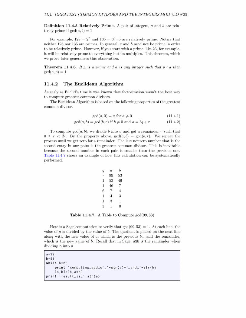
As early as Euclid’s time it was known that factorization wasn’t the best wayto compute greatest common divisors.
The Euclidean Algorithm is based on the following properties of the greatestcommon divisor.
gcd(a, 0) = a for a 6= 0 (11.4.1)gcd(a, b) = gcd(b, r) if b 6= 0 and a = bq + r (11.4.2)
To compute gcd(a, b), we divide b into a and get a remainder r such that0 ≤ r < |b|. By the property above, gcd(a, b) = gcd(b, r). We repeat theprocess until we get zero for a remainder. The last nonzero number that is thesecond entry in our pairs is the greatest common divisor. This is inevitablebecause the second number in each pair is smaller than the previous one.Table 11.4.7 shows an example of how this calculation can be systematicallyperformed.
q a b
- 99 531 53 461 46 76 7 41 4 31 3 13 1 0
Table 11.4.7: A Table to Compute gcd(99, 53)
Here is a Sage computation to verify that gcd(99, 53) = 1. At each line, thevalue of a is divided by the value of b. The quotient is placed on the next linealong with the new value of a, which is the previous b;. and the remainder,which is the new value of b. Recall that in Sage, a%b is the remainder whendividing b into a.
a=99b=53while b>0:
print 'computing␣gcd␣of␣'+str(a)+'␣and␣'+str(b)[a,b]=[b,a%b]
print 'result␣is␣'+str(a)
36 CHAPTER 11. ALGEBRAIC STRUCTURES
computing gcd of 99 and 53computing gcd of 53 and 46computing gcd of 46 and 7computing gcd of 7 and 4computing gcd of 4 and 3computing gcd of 3 and 1result is 1
Investigation 11.4.1. If you were allowed to pick two numbers less than 100,which would you pick in order to force Euclid to work hardest? Here’s a hint:The size of the quotient at each step determines how quickly the numbersdecrease.Solution. If quotient in division is 1, then we get the slowest possible com-pletion. If a = b + r, then working backwards, each remainder would be thesum of the two previous remainders. This described a sequence like the Fi-bonacci sequence and indeed, the greatest common divisor of two consecutiveFibonacci numbers will take the most steps to reach a final value of 1.
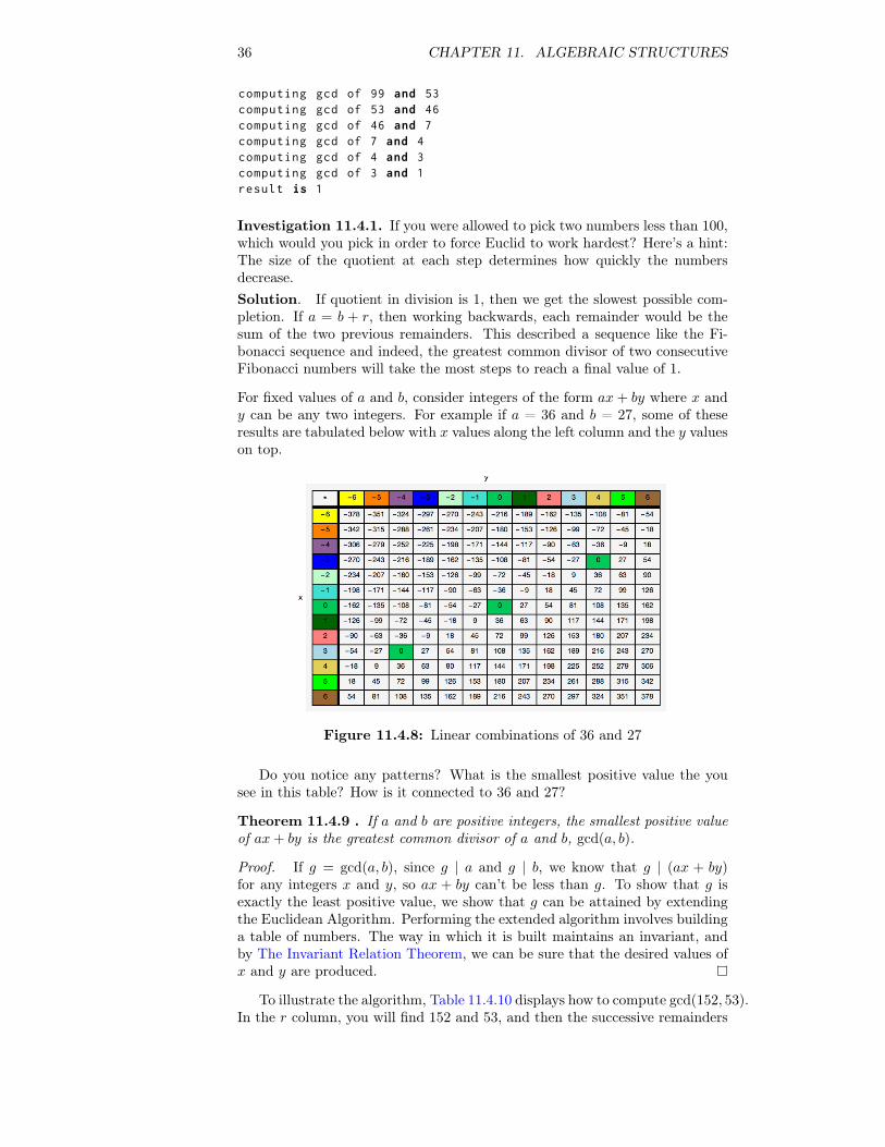
For fixed values of a and b, consider integers of the form ax+ by where x andy can be any two integers. For example if a = 36 and b = 27, some of theseresults are tabulated below with x values along the left column and the y valueson top.
Figure 11.4.8: Linear combinations of 36 and 27
Do you notice any patterns? What is the smallest positive value the yousee in this table? How is it connected to 36 and 27?
Theorem 11.4.9 . If a and b are positive integers, the smallest positive valueof ax+ by is the greatest common divisor of a and b, gcd(a, b).
Proof. If g = gcd(a, b), since g | a and g | b, we know that g | (ax + by)for any integers x and y, so ax + by can’t be less than g. To show that g isexactly the least positive value, we show that g can be attained by extendingthe Euclidean Algorithm. Performing the extended algorithm involves buildinga table of numbers. The way in which it is built maintains an invariant, andby The Invariant Relation Theorem, we can be sure that the desired values ofx and y are produced.
To illustrate the algorithm, Table 11.4.10 displays how to compute gcd(152, 53).In the r column, you will find 152 and 53, and then the successive remainders
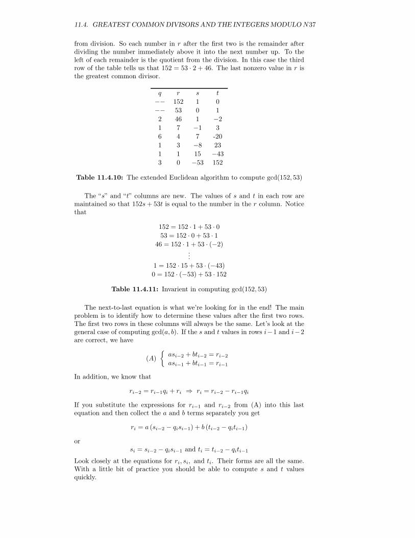
11.4. GREATEST COMMON DIVISORS AND THE INTEGERS MODULON37
from division. So each number in r after the first two is the remainder afterdividing the number immediately above it into the next number up. To theleft of each remainder is the quotient from the division. In this case the thirdrow of the table tells us that 152 = 53 · 2 + 46. The last nonzero value in r isthe greatest common divisor.
q r s t
−− 152 1 0−− 53 0 12 46 1 −2
1 7 −1 36 4 7 -201 3 −8 231 1 15 −43
3 0 −53 152
Table 11.4.10: The extended Euclidean algorithm to compute gcd(152, 53)
The “s” and “t” columns are new. The values of s and t in each row aremaintained so that 152s+ 53t is equal to the number in the r column. Noticethat
152 = 152 · 1 + 53 · 053 = 152 · 0 + 53 · 1
46 = 152 · 1 + 53 · (−2)...
1 = 152 · 15 + 53 · (−43)
0 = 152 · (−53) + 53 · 152
Table 11.4.11: Invarient in computing gcd(152, 53)
The next-to-last equation is what we’re looking for in the end! The mainproblem is to identify how to determine these values after the first two rows.The first two rows in these columns will always be the same. Let’s look at thegeneral case of computing gcd(a, b). If the s and t values in rows i−1 and i−2are correct, we have
(A)
{asi−2 + bti−2 = ri−2
asi−1 + bti−1 = ri−1
In addition, we know that
ri−2 = ri−1qi + ri ⇒ ri = ri−2 − ri−1qi
If you substitute the expressions for ri−1 and ri−2 from (A) into this lastequation and then collect the a and b terms separately you get
ri = a (si−2 − qisi−1) + b (ti−2 − qiti−1)
orsi = si−2 − qisi−1 and ti = ti−2 − qiti−1
Look closely at the equations for ri, si, and ti. Their forms are all the same.With a little bit of practice you should be able to compute s and t valuesquickly.
38 CHAPTER 11. ALGEBRAIC STRUCTURES
11.4.3 Modular Arithmetic
We remind you of the relation on the integers that we call Definition 6.0.2. Iftwo numbers, a and b, differ by a multiple of n, we say that they are congruentmodulo n, denoted a ≡ b (mod n). For example, 13 ≡ 38 (mod 5) because13− 38 = −25, which is a multiple of 5.
Definition 11.4.12 Modular Addition. If n is a positive integer, we defineaddition modulo n (+n ) as follows. If a, b ∈ Z,
a+n b = the remainder after a+ b is divided by n
Definition 11.4.13 Modular Multiplication. If n is a positive integer, wedefine multiplication modulo n (×n ) as follows. If a, b ∈ Z,
a×n b = the remainder after a · b is divided by n
Note 11.4.14.
(a) The result of doing arithmetic modulo n is always an integer between0 and n − 1, by the Division Property. This observation implies that{0, 1, . . . , n− 1} is closed under modulo n arithmetic.
(b) It is always true that a +n b ≡ (a + b) (mod n) and a ×n b ≡ (a · b)(mod n). For example, 4 +7 5 = 2 ≡ 9 (mod 7) and 4 ×7 5 ≡ 6 ≡ 20(mod 7).
(c) We will use the notation Zn to denote the set {0, 1, 2, ..., n− 1}.
11.4.4 Properties of Modular Arithmetic
Theorem 11.4.15 Additive Inverses in Zn. If a ∈ Zn, a 6= 0, then theadditive inverse of a is n− a.
Proof. a+(n−a) = n ≡ 0( mod n), since n = n·1+0. Therefore, a+n(n−a) =0.
Addition modulo n is always commutative and associative; 0 is the identityfor +n and every element of Zn has an additive inverse. These properties canbe summarized by noting that for each n ≥ 1, [Zn; +n] is a group.
Definition 11.4.16 The Additive Group of Integers Modulo n. TheAdditive Group of Integers Modulo n is the group with elements {0, 1, 2, . . . , n−1} and with the operation of mod n addition. It is denoted as Zn.
Multiplication modulo n is always commutative and associative, and 1 isthe identity for ×n.
Notice that the algebraic properties of +n and ×n on Zn are identical tothe properties of addition and multiplication on Z.
Notice that a group cannot be formed from the whole set {0, 1, 2, . . . , n −1} with mod n multiplication since zero never has a multiplicative inverse.Depending on the value of n there may be other restrictions. The followinggroup will be explored in Exercise 9.
Definition 11.4.17 The Multiplicative Group of Integers Modulo n.The Multiplicative Group of Integers Modulo n is the group with elements{k ∈ Z|1 ≤ k ≤ n − 1 and gcd(n, k) = 1} and with the operation of mod nMultiplication. It is denoted as Un.
11.4. GREATEST COMMON DIVISORS AND THE INTEGERS MODULON39
Example 11.4.18 Some Examples.
(a) We are all somewhat familiar with Z12 since the hours of the day arecounted using this group, except for the fact that 12 is used in place of 0.Military time uses the mod 24 system and does begin at 0. If someonestarted a four-hour trip at hour 21, the time at which she would arriveis 21 +24 4 = 1. If a satellite orbits the earth every four hours and startsits first orbit at hour 5, it would end its first orbit at time 5 +24 4 = 9.Its tenth orbit would end at 5 +24 10×24 4 = 21 hours on the clock
(b) Virtually all computers represent unsigned integers in binary form witha fixed number of digits. A very small computer might reserve seven bitsto store the value of an integer. There are only 27 different values thatcan be stored in seven bits. Since the smallest value is 0, represented as0000000, the maximum value will be 27−1 = 127, represented as 1111111.When a command is given to add two integer values, and the two valueshave a sum of 128 or more, overflow occurs. For example, if we try toadd 56 and 95, the sum is an eight-digit binary integer 10010111. Onecommon procedure is to retain the seven lowest-ordered digits. The resultof adding 56 and 95 would be 0010111 two = 23 ≡ 56 + 95 (mod 128).Integer arithmetic with this computer would actually be modulo 128arithmetic.
11.4.5 SageMath Note - Modular ArithmeticSage inherits the basic integer division functions from Python that compute aquotient and remainder in integer division. For example, here is how to divide561 into 2017 and get the quotient and remainder.
a=2017b=561[q,r]=[a//b,a%b][q,r]
[3, 334]
In Sage, gcd is the greatest common divisor function. It can be used intwo ways. For the gcd of 2343 and 4319 we can evaluate the expressiongcd(2343, 4319). If we are working with a fixed modulus m that has a value es-tablished in your Sage session, the expressionm.gcd(k) to compute the greatestcommon divisor of m and any integer value k. The extended Euclidean algo-rithm can also be called upon with xgcd:
a=2017b=561print gcd(a,b)print xgcd(a,b)
1(1, -173, 622)
Sage has some extremely powerful tool for working with groups. The integersmodulo n are represented by the expression Integers(n) and the addition andmultiplications tables can be generated as follows.
R = Integers (6)print R.addition_table('elements ')print R.multiplication_table('elements ')
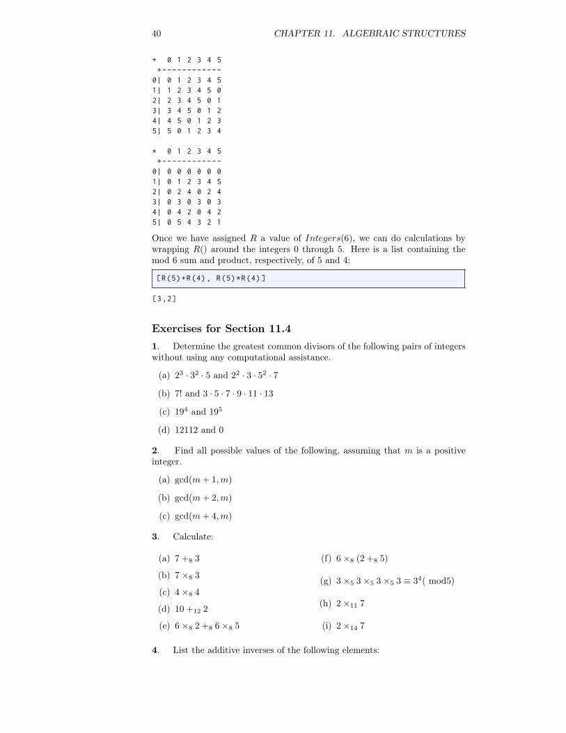
40 CHAPTER 11. ALGEBRAIC STRUCTURES
+ 0 1 2 3 4 5+------------
0| 0 1 2 3 4 51| 1 2 3 4 5 02| 2 3 4 5 0 13| 3 4 5 0 1 24| 4 5 0 1 2 35| 5 0 1 2 3 4
* 0 1 2 3 4 5+------------
0| 0 0 0 0 0 01| 0 1 2 3 4 52| 0 2 4 0 2 43| 0 3 0 3 0 34| 0 4 2 0 4 25| 0 5 4 3 2 1
Once we have assigned R a value of Integers(6), we can do calculations bywrapping R() around the integers 0 through 5. Here is a list containing themod 6 sum and product, respectively, of 5 and 4:
[R(5)+R(4), R(5)*R(4)]
[3,2]
Exercises for Section 11.41. Determine the greatest common divisors of the following pairs of integerswithout using any computational assistance.
(a) 23 · 32 · 5 and 22 · 3 · 52 · 7
(b) 7! and 3 · 5 · 7 · 9 · 11 · 13
(c) 194 and 195
(d) 12112 and 0
2. Find all possible values of the following, assuming that m is a positiveinteger.
(a) gcd(m+ 1,m)
(b) gcd(m+ 2,m)
(c) gcd(m+ 4,m)
3. Calculate:
(a) 7 +8 3
(b) 7×8 3
(c) 4×8 4
(d) 10 +12 2
(e) 6×8 2 +8 6×8 5
(f) 6×8 (2 +8 5)
(g) 3×5 3×5 3×5 3 ≡ 34( mod5)
(h) 2×11 7
(i) 2×14 7
4. List the additive inverses of the following elements:
11.5. SUBSYSTEMS 41
(a) 4, 6, 9 in Z10
(b) 16, 25, 40 in Z50
5. In the group Z11 , what are:
(a) 3(4)?
(b) 36(4)?
(c) How could you efficiently compute m(4), m ∈ Z?
6. Prove that {1, 2, 3, 4} is a group under the operation ×5.7. A student is asked to solve the following equations under the requirementthat all arithmetic should be done in Z2. List all solutions.
(a) x2 + 1 = 0.
(b) x2 + x+ 1 = 0.
8. Determine the solutions of the same equations as in Exercise 5 in Z5.9.
(a) Write out the operation table for ×8 on {1, 3, 5, 7}, and convince yourself that this is a group.
(b) Let Un be the elements of Zn that have inverses with respect to ×n.Convince yourself that Un is a group under ×n.
(c) Prove that the elements of Un are those elements a ∈ Zn such thatgcd(n, a) = 1. You may use Theorem 11.4.9 in this proof.
10. Prove the division property, Theorem 11.4.1.Hint. Prove by induction on m that you can divide any positive integer intom. That is, let p(m) be “For all n greater than zero, there exist unique integersq and r such that . . . .” In the induction step, divide n into m− n.11. Suppose f : Z17 → Z17 such f(i) = a ×17 i +17 b where a and b areinteger constants. Furthermore, assume that f(1) = 11 and f(2) = 4. Find aformula for f(i) and also find a formula for the inverse of f .
11.5 Subsystems
11.5.1 DefinitionThe subsystem is a fundamental concept of algebra at the universal level.
Definition 11.5.1 Subsystem. If [V ; ∗1, . . . , ∗n] is an algebraic system ofa certain kind and W is a subset of V , then W is a subsystem of V if[W ; ∗1, . . . , ∗n] is an algebraic system of the same kind as V . The usual nota-tion for “W is a subsystem of V ” is W ≤ V .
Since the definition of a subsystem is at the universal level, we can citeexamples of the concept of subsystems at both the axiomatic and concretelevel.
Example 11.5.2 Examples of Subsystems.
42 CHAPTER 11. ALGEBRAIC STRUCTURES
(a) (Axiomatic) If [G; ∗] is a group, and H is a subset of G, then H is asubgroup of G if [H; ∗] is a group.
(b) (Concrete) U = {−1, 1} is a subgroup of [R∗; ·]. Take the time now towrite out the multiplication table of U and convince yourself that [U ; ·]is a group.
(c) (Concrete) The even integers, 2Z = {2k : k is an integer} is a subgroupof [Z; +]. Convince yourself of this fact.
(d) (Concrete) The set of nonnegative integers is not a subgroup of [Z; +].All of the group axioms are true for this subset except one: no positiveinteger has a positive additive inverse. Therefore, the inverse property isnot true. Note that every group axiom must be true for a subset to be asubgroup.
(e) (Axiomatic) If M is a monoid and P is a subset of M , then P is asubmonoid of M if P is a monoid.
(f) (Concrete) If B∗ is the set of strings of 0’s and 1’s of length zero or morewith the operation of concatenation, then two examples of submonoidsof B∗ are: (i) the set of strings of even length, and (ii) the set of stringsthat contain no 0’s. The set of strings of length less than 50 is not asubmonoid because it isn’t closed under concatenation. Why isn’t theset of strings of length 50 or more a submonoid of B∗?
11.5.2 SubgroupsFor the remainder of this section, we will concentrate on the properties ofsubgroups. The first order of business is to establish a systematic way ofdetermining whether a subset of a group is a subgroup.
Theorem 11.5.3 Subgroup Conditions. To determine whether H, a subsetof group [G; ∗], is a subgroup, it is sufficient to prove:
(a) H is closed under ∗; that is, a, b ∈ H ⇒ a ∗ b ∈ H;
(b) H contains the identity element for ∗; and
(c) H contains the inverse of each of its elements; that is, a ∈ H ⇒ a−1 ∈ H.
Proof. Our proof consists of verifying that if the three properties above aretrue, then all the axioms of a group are true for [H; ∗]. By Condition (a), ∗can be considered an operation on H. The associative, identity, and inverseproperties are the axioms that are needed. The identity and inverse propertiesare true by conditions (b) and (c), respectively, leaving only the associativeproperty. Since, [G; ∗] is a group, a ∗ (b ∗ c) = (a ∗ b) ∗ c for all a, b, c ∈ G.Certainly, if this equation is true for all choices of three elements from G, itwill be true for all choices of three elements from H, since H is a subset ofG.
For every group with at least two elements, there are at least two subgroups:they are the whole group and {e}. Since these two are automatic, they are notconsidered very interesting and are called the improper subgroups of the group;{e} is sometimes referred to as the trivial subgroup. All other subgroups, ifthere are any, are called proper subgroups.
We can apply Theorem 11.5.3 at both the concrete and axiomatic levels.
Example 11.5.4 Applying Conditions for a Subgroup.
11.5. SUBSYSTEMS 43
(a) (Concrete) We can verify that 2Z ≤ Z, as stated in Example 11.5.2.Whenever you want to discuss a subset, you must find some convenientway of describing its elements. An element of 2Z can be described as 2times an integer; that is, a ∈ 2Z is equivalent to (∃k)Z(a = 2k). Nowwe can verify that the three conditions of Theorem 11.5.3 are true for2Z. First, if a, b ∈ 2Z, then there exist j, k ∈ Z such that a = 2j andb = 2k. A common error is to write something like a = 2j and b = 2j.This would mean that a = b, which is not necessarily true. That is whytwo different variables are needed to describe a and b. Returning to ourproof, we can add a and b: a + b = 2j + 2k = 2(j + k). Since j + k isan integer, a + b is an element of 2Z. Second, the identity, 0, belongsto 2Z (0 = 2(0)). Finally, if a ∈ 2Z and a = 2k,−a = −(2k) = 2(−k),and −k ∈ Z, therefore, −a ∈ 2Z. By Theorem 11.5.3, 2Z ≤ Z. Howwould this argument change if you were asked to prove that 3Z ≤ Z? ornZ ≤ Z, n ≥ 2?
(b) (Concrete) We can prove that H = {0, 3, 6, 9} is a subgroup of Z12. First,for each ordered pair (a, b) ∈ H×H, a+12 b is in H. This can be checkedwithout too much trouble since |H ×H| = 16. Thus we can concludethat H is closed under +12. Second, 0 ∈ H. Third, −0 = 0, −3 = 9,−6 = 6, and −9 = 3. Therefore, the inverse of each element of H is inH.
(c) (Axiomatic) IfH andK are both subgroups of a group G, thenH∩K is asubgroup ofG. To justify this statement, we have no concrete informationto work with, only the facts that H ≤ G and K ≤ G. Our proof thatH ∩K ≤ G reflects this and is an exercise in applying the definitions ofintersection and subgroup, (i) If a and b are elements of H ∩K, then aand b both belong to H, and since H ≤ G, a∗b must be an element of H.Similarly, a ∗ b ∈ K; therefore, a ∗ b ∈ H ∩K. (ii) The identity of G mustbelong to both H and K; hence it belongs to H ∩K. (iii) If a ∈ H ∩K,then a ∈ H, and since H ≤ G, a−1 ∈ H. Similarly, a−1 ∈ K. Hence, bythe theorem, H ∩K ≤ G. Now that this fact has been established, wecan apply it to any pair of subgroups of any group. For example, since2Z and 3Z are both subgroups of [Z; +], 2Z∩ 3Z is also a subgroup of Z.Note that if a ∈ 2Z ∩ 3Z, a must have a factor of 3; that is, there existsk ∈ Z such that a = 3k. In addition, a must be even, therefore k mustbe even. There exists j ∈ Z such that k = 2j, therefore a = 3(2j) = 6j.This shows that 2Z ∩ 3Z ⊆ 6Z. The opposite containment can easily beestablished; therefore, 2Z ∩ 3Z = 6Z.
Given a finite group, we can apply Theorem 11.3.15 to obtain a simplercondition for a subset to be a subgroup.
Theorem 11.5.5 Condition for a Subgroup of Finite Group. Given that[G; ∗] is a finite group and H is a nonempty subset of G, if H is closed under∗ , then H is a subgroup of G.
Proof. In this proof, we demonstrate that Conditions (b) and (c) of Theo-rem 11.5.3 follow from the closure of H under ∗, which is condition (a) of thetheorem. First, select any element of H; call it β. The powers of β : β1, β2,β3, . . . are all in H by the closure property. By Theorem 11.3.15, there existsm, m ≤ |G|, such that βm = e; hence e ∈ H. To prove that (c) is true, we leta be any element of H. If a = e, then a−1 is in H since e−1 = e. If a 6= e,aq = e for some q between 2 and |G| and
e = aq = aq−1 ∗ a
44 CHAPTER 11. ALGEBRAIC STRUCTURES
Therefore, a−1 = aq−1 , which belongs to H since q − 1 ≥ 1.
11.5.3 Sage Note - Applying the condition for a subgroupof a finite group
To determine whether H1 = {0, 5, 10} and H2 = {0, 4, 8, 12} are subgroups ofZ15, we need only write out the addition tables (modulo 15) for these sets.This is easy to do with a bit of Sage code that we include below and then forany modulus and subset, we can generate the body of an addition table. Thecode is set up for H1 but can be easily adjusted for H2.
def addition_table(n,H):for a in H:
line =[]for b in H:
line +=[(a+b)%n]print line
addition_table (15,Set ([0 ,5 ,10]))
[0, 10, 5][10, 5, 0][5, 0, 10]
Note that H1 is a subgroup of Z15. Since the interior of the addition table forH2 contains elements that are outside of H2, H2 is not a subgroup of Z15.
11.5.4 Cyclic SubgroupsOne kind of subgroup that merits special mention due to its simplicity is thecyclic subgroup.
Definition 11.5.6 Cyclic Subgroup. If G is a group and a ∈ G, the cyclicsubgroup generated by a, 〈a〉, is the set of all powers of a:
〈a〉 = {an : n ∈ Z} .
We refer to a as a generator of subgroup 〈a〉.A subgroupH of a group G is cyclic if there exists a ∈ H such thatH = 〈a〉.
Definition 11.5.7 Cyclic Group. A group G is cyclic if there exists β ∈ Gsuch that 〈β〉 = G.
Note 11.5.8. If the operation on G is additive, then 〈a〉 = {(n)a : n ∈ Z}.
Definition 11.5.9 Order of a Group Element. The order of an elementa of group G is the number of elements in the cyclic subgroup of G generatedby a. The order of a is denoted ord(a).
Example 11.5.10.
(a) In [R∗; ·], 〈2〉 = {2n : n ∈ Z} ={. . . , 1
16 ,18 ,
14 ,
12 , 1, 2, 4, 8, 16, . . .
}.
(b) In Z15, 〈6〉 = {0, 3, 6, 9, 12}. If G is finite, you need list only the positivepowers (or multiples) of a up to the first occurrence of the identity toobtain all of 〈a〉. In Z15 , the multiples of 6 are 6, (2)6 = 12, (3)6 = 3,(4)6 = 9, and (5)6 = 0. Note that {0, 3, 6, 9, 12} is also 〈3〉,〈9〉, and 〈12〉.This shows that a cyclic subgroup can have different generators.
If you want to list the cyclic subgroups of a group, the following theoremcan save you some time.
11.5. SUBSYSTEMS 45
Theorem 11.5.11. If a is an element of group G, then 〈a〉 = 〈a−1〉.
This is an easy way of seeing, for example, that 〈9〉 in Z15 equals 〈6〉, since−6 = 9.
Exercises for Section 11.51. Which of the following subsets of the real numbers is a subgroup of [R; +]?
(a) the rational numbers
(b) the positive real numbers
(c) {k/2 | k is an integer}
(d) {2k | k is an integer}
(e) {x | −100 ≤ x ≤ 100}
2. Describe in simpler terms the following subgroups of Z:
(a) 5Z ∩ 4Z
(b) 4Z ∩ 6Z (be careful)
(c) the only finite subgroup of Z
3. Find at least two proper subgroups of R3 , the set of 3× 3 rook matrices(see Exercise 11.2.5).4. Where should you place the following in Figure 11.5.12?
(a) e
(b) a−1
(c) x ∗ y
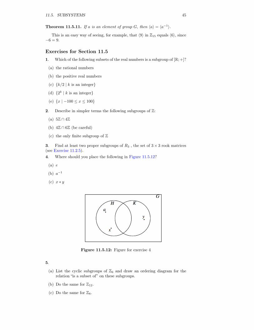
Figure 11.5.12: Figure for exercise 4
5.
(a) List the cyclic subgroups of Z6 and draw an ordering diagram for therelation “is a subset of” on these subgroups.
(b) Do the same for Z12.
(c) Do the same for Z8.
46 CHAPTER 11. ALGEBRAIC STRUCTURES
(d) On the basis of your results in parts a, b, and c, what would you expectif you did the same with Z24?
6. Subgroups generated by subsets of a group. The concept of a cyclicsubgroup is a special case of the concept that we will discuss here. Let [G; ∗]be a group and S a nonempty subset of G. Define the set 〈S〉 recursively by:
• If a ∈ S, then a ∈ 〈S〉.
• If a, b ∈ 〈S〉, then a ∗ b ∈ 〈S〉, and
• If a ∈ 〈S〉, then a−1 ∈ 〈S〉.
(a) By its definition, 〈S〉 has all of the properties needed to be a subgroup ofG. The only thing that isn’t obvious is that the identity of G is in 〈S〉.Prove that the identity of G is in 〈S〉.
(b) What is 〈{9, 15}〉 in[Z; +]?
(c) Prove that if H ≤ G and S ⊆ H, then 〈S〉 ≤ H. This proves that〈S〉 is contained in every subgroup of G that contains S; that is, 〈S〉 =∩
S⊆H,H≤GH.
(d) Describe 〈{0.5, 3}〉 in [R+; ·] and in [R; +].
(e) If j, k ∈ Z, 〈{j, k}〉 is a cyclic subgroup of Z. In terms of j and k, whatis a generator of 〈{j, k}〉?
7. Prove that if H,K ≤ G, and H ∪K = G, then H = G or K = G.Hint. Use an indirect argument.8. Prove that the order of an element, a of a group is the least positiveinteger, k, such that ak is the identity of the group.
11.6 Direct Products
11.6.1 DefinitionOur second universal algebraic concept lets us look in the opposite directionfrom subsystems. Direct products allow us to create larger systems. In thefollowing definition, we avoid complicating the notation by not specifying howmany operations the systems have.
Definition 11.6.1 Direct Product. If [Vi; ∗i, �i, . . .], i = 1, 2, . . . , n are al-gebraic systems of the same kind, then the direct product of these systems isV = V1×V2×· · ·×Vn , with operations defined below. The elements of V aren-tuples of the form (a1, a2, . . . , an), where ak ∈ Vk, k = 1, . . . , n. The systemsV1, V2, . . . , Vn are called the factors of V . There are as many operations on Vas there are in the factors. Each of these operations is defined componentwise:
If (a1, a2, ..., an) , (b1, b2, ..., bn) ∈ V ,
(a1, a2, . . . , an) ∗ (b1, b2, . . . , bn) = (a1 ∗1 b1, a2 ∗2 b2, . . . , an ∗n bn)
(a1, a2, . . . , an) � (b1, b2, . . . , bn) = (a1 �1 b1, a2 �2 b2, . . . , an �n bn)
etc.
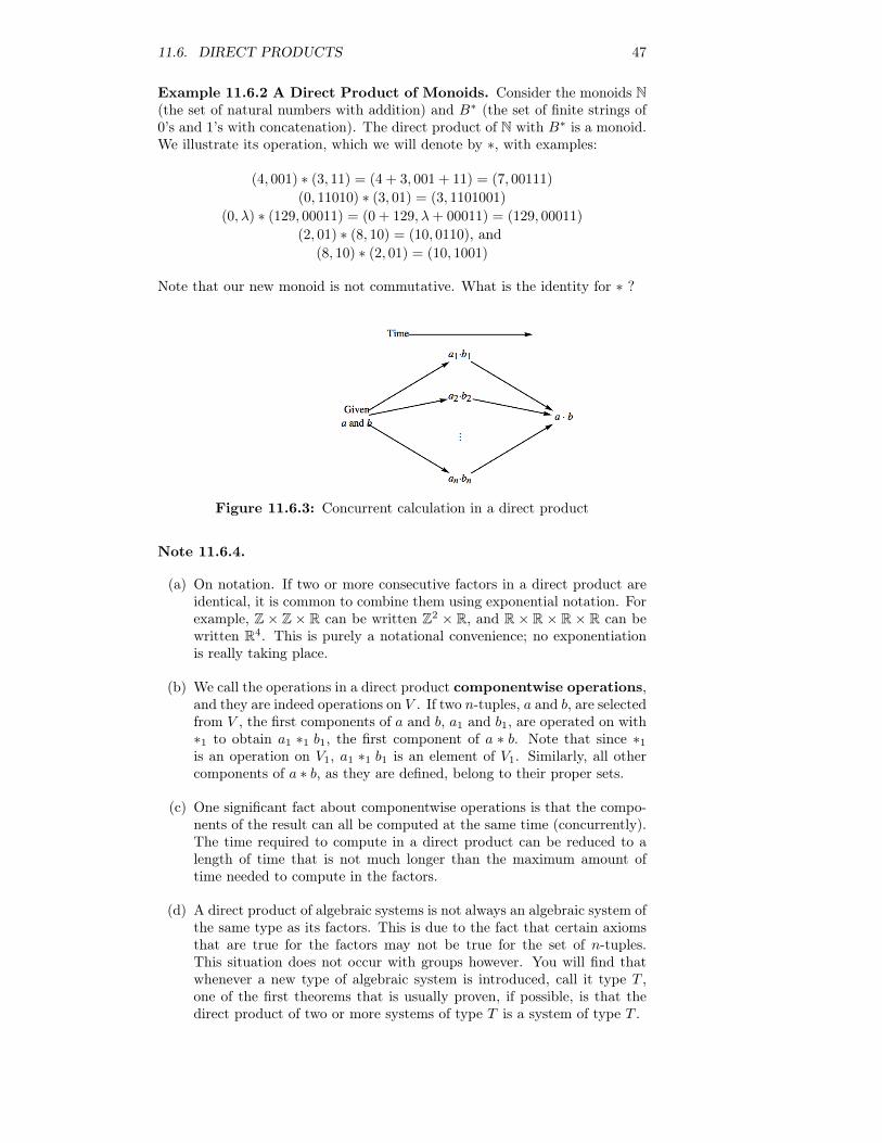
11.6. DIRECT PRODUCTS 47
Example 11.6.2 A Direct Product of Monoids. Consider the monoids N(the set of natural numbers with addition) and B∗ (the set of finite strings of0’s and 1’s with concatenation). The direct product of N with B∗ is a monoid.We illustrate its operation, which we will denote by ∗, with examples:
(4, 001) ∗ (3, 11) = (4 + 3, 001 + 11) = (7, 00111)
(0, 11010) ∗ (3, 01) = (3, 1101001)
(0, λ) ∗ (129, 00011) = (0 + 129, λ+ 00011) = (129, 00011)
(2, 01) ∗ (8, 10) = (10, 0110), and(8, 10) ∗ (2, 01) = (10, 1001)
Note that our new monoid is not commutative. What is the identity for ∗ ?
Figure 11.6.3: Concurrent calculation in a direct product
Note 11.6.4.
(a) On notation. If two or more consecutive factors in a direct product areidentical, it is common to combine them using exponential notation. Forexample, Z × Z × R can be written Z2 × R, and R × R × R × R can bewritten R4. This is purely a notational convenience; no exponentiationis really taking place.
(b) We call the operations in a direct product componentwise operations,and they are indeed operations on V . If two n-tuples, a and b, are selectedfrom V , the first components of a and b, a1 and b1, are operated on with∗1 to obtain a1 ∗1 b1, the first component of a ∗ b. Note that since ∗1is an operation on V1, a1 ∗1 b1 is an element of V1. Similarly, all othercomponents of a ∗ b, as they are defined, belong to their proper sets.
(c) One significant fact about componentwise operations is that the compo-nents of the result can all be computed at the same time (concurrently).The time required to compute in a direct product can be reduced to alength of time that is not much longer than the maximum amount oftime needed to compute in the factors.
(d) A direct product of algebraic systems is not always an algebraic system ofthe same type as its factors. This is due to the fact that certain axiomsthat are true for the factors may not be true for the set of n-tuples.This situation does not occur with groups however. You will find thatwhenever a new type of algebraic system is introduced, call it type T ,one of the first theorems that is usually proven, if possible, is that thedirect product of two or more systems of type T is a system of type T .
48 CHAPTER 11. ALGEBRAIC STRUCTURES
11.6.2 Direct Products of GroupsTheorem 11.6.5 The Direct Product of Groups is a Group. The directproduct of two or more groups is a group; that is, the algebraic properties ofa system obtained by taking the direct product of two or more groups includesthe group axioms.
Proof. We will only present the proof of this theorem for the direct productof two groups. Some slight revisions can be made to produce a proof for anynumber of factors.
Stating that the direct product of two groups is a group is a short way ofsaying that if [G1; ∗1] and [G2; ∗2] are groups, then [G1 ×G2; ∗] is also a group,where ∗ is the componentwise operation on G1 × G2. Associativity of ∗ : Ifa, b, c ∈ G1 ×G2,
a ∗ (b ∗ c) = (a1, a2) ∗ ((b1, b2) ∗ (c1, c2))
= (a1, a2) ∗ (b1 ∗1 c1, b2 ∗2 c2)
= (a1 ∗1 (b1 ∗1 c1) , a2 ∗2 (b2 ∗2 c2))
= ((a1 ∗1 b1) ∗1 c1, (a2 ∗2 b2) ∗2 c2)
= (a1 ∗1 b1, a2 ∗2 b2) ∗ (c1, c2)
= ((a1, a2) ∗ (b1, b2)) ∗ (c1, c2)
= (a ∗ b) ∗ c
Notice how the associativity property hinges on the associativity in each factor.An identity for ∗: As you might expect, if e1 and e2 are identities for G1 andG2, respectively, then e = (e1, e2) is the identity for G1 ×G2. If a ∈ G1 ×G2,
a ∗ e = (a1, a2) ∗ (e1, e2)
= (a1 ∗1 e1, a2 ∗2 e2)
= (a1, a2) = a
Similarly, e ∗ a = a.Inverses in G1×G2: The inverse of an element is determined componentwise
a−1 = (a1, a2)−1 =(a1−1, a2
−1). To verify, we compute a ∗ a−1 :
a ∗ a−1 = (a1, a2) ∗(a1−1, a2
−1)
=(a1 ∗1 a1
−1, a2 ∗2 a2−1)
= (e1, e2) = e
Similarly, a−1 ∗ a = e.
Example 11.6.6 Some New Groups.
(a) If n ≥ 2, Z2n , the direct product of n factors of Z2, is a group with
2n elements. We will take a closer look at Z23 = Z2 × Z2 × Z2. The
elements of this group are triples of zeros and ones. Since the operationon Z2 is +2, we will use the symbol + for the operation on Z2
3 . Twoof the eight triples in the group are a = (1, 0, 1) and b = (0, 0, 1). Their“sum” is a + b = (1 +2 0, 0 +2 0, 1 +2 1) = (1, 0, 0). One interesting factabout this group is that each element is its own inverse. For examplea + a = (1, 0, 1) + (1, 0, 1) = (0, 0, 0); therefore −a = a. We use theadditive notation for the inverse of a because we are using a form ofaddition. Note that {(0, 0, 0), (1, 0, 1)} is a subgroup of Z2
3. Write outthe “addition” table for this set and apply Theorem 11.5.5. The samecan be said for any set consisting of (0, 0, 0) and another element of Z2
3.
11.6. DIRECT PRODUCTS 49
(b) The direct product of the positive real numbers with the integers modulo4, R+ × Z4 is an infinite group since one of its factors is infinite. Theoperations on the factors are multiplication and modular addition, so wewill select the neutral symbol � for the operation on R+×Z4. If a = (4, 3)and b = (0.5, 2), then
a � b = (4, 3) � (0.5, 2) = (4 · 0.5, 3 +4 2) = (2, 1)
b2 = b � b = (0.5, 2) � (0.5, 2) = (0.25, 0)
a−1 =(4−1,−3
)= (0.25, 1)
b−1 =(0.5−1,−2
)= (2, 2)
It would be incorrect to say that Z4 is a subgroup of R+ × Z4 , butthere is a subgroup of the direct product that closely resembles Z4. It is{(1, 0), (1, 1), (1, 2), (1, 3)}. Its table is
� (1, 0) (1, 1) (1, 2) (1, 3)
(1, 0) (1, 0) (1, 1) (1, 2) (1, 3)
(1, 1) (1, 1) (1, 2) (1, 3) (1, 0)
(1, 2) (1, 2) (1, 3) (1, 0) (1, 1)
(1, 3) (1, 3) (1, 0) (1, 1) (1, 2)
Imagine erasing (1, ) throughout the table and writing +4 in place of �.What would you get? We will explore this phenomenon in detail in thenext section.The whole direct product could be visualized as four parallel half-lineslabeled 0, 1, 2, and 3 as in Figure 11.6.7. On the kth line, the pointthat lies x units to the right of the zero mark would be (x, k). The set{(2n, (n)1) | n ∈ Z}, which is depicted on the figure is a subgroup ofR+ × Z4. What cyclic subgroup is it?The answer: 〈(2, 1)〉 or 〈(1/2, 3)〉. There are two different generators.
Figure 11.6.7: Visualization of the group R+ × Z4
A more conventional direct product is R2, the direct product of two factorsof [R; +]. The operation on R2 is componentwise addition; hence we will use+ as the operation symbol for this group. You should be familiar with thisoperation, since it is identical to addition of 2 × 1 matrices. The Cartesiancoordinate system can be used to visualize R2 geometrically. We plot the pair(s, t) on the plane in the usual way: s units along the x axis and t units alongthe y axis. There is a variety of different subgroups of R2 , a few of which are:
50 CHAPTER 11. ALGEBRAIC STRUCTURES
(a) {(x, 0) | x ∈ R}, all of the points on the x axis;
(b) {(x, y) | 2x− y = 0}, all of the points that are on the line 2x - y = 0;
(c) If a, b ∈ R, {(x, y) | ax + by = 0}. The first two subgroups are specialcases of this one, which represents any line that passes through the origin.
(d) {(x, y) | 2x− y = k, k ∈ Z}, a union of a set of lines that are parallel to2x− y = 0.
(e) {(n, 3n) | n ∈ Z}, which is the only countable subgroup that we havelisted.
We will leave it to the reader to verify that these sets are subgroups. We willonly point out how the fourth example, call it H, is closed under “addition.” Ifa = (p, q) and b = (s, t) and both belong to H, then 2p− q = j and 2s− t = k,where both j and k are integers. a+ b = (p, q) + (s, t) = (p+ s, q + t) We candetermine whether a+b belongs toH by deciding whether or not 2(p+s)−(q+t)is an integer:
2(p+ s)− (q + t) = 2p+ 2s− q − t= (2p− q) + (2s− t)= j + k
Since j and k are integers, so is j+ k. This completes a proof that H is closedunder the operation of R2.
Several useful facts can be stated in regards to the direct product of two ormore groups. We will combine them into one theorem, which we will presentwith no proof. Parts a and c were derived for n = 2 in the proof of Theo-rem 11.6.5.
Theorem 11.6.8 Properties of Direct Products of Groups. If G =G1 × G2 × · · · × Gn is a direct product of n groups and (a1, a2, . . . , an) ∈ G,then:
(a) The identity of G is (e1, e2, ..., en), where ek, is the identity of Gk.
(b) (a1, a2, ..., an)−1 =(a1−1, a2
−1, ..., an−1).
(c) (a1, a2, ..., an)m = (a1m, a2
m, ..., anm) for all m ∈ Z.
(d) G is abelian if and only if each of the factors G1, G2, . . . , Gn is abelian.
(e) lf H1, H2, . . . ,Hn are subgroups of the corresponding factors, then H1 ×H2 × · · · ×Hn is a subgroup of G.
Not all subgroups of a direct product can be created using part e of The-orem 11.6.8. For example, {(n, n) | n ∈ Z} is a subgroup of Z2, but is not adirect product of two subgroups of Z.
Example 11.6.9 Linked Lists using a Direct Product. Using the identity(x+y)+x = y, in Z2, we can devise a scheme for representing a symmetricallylinked list using only one link field. A symmetrically linked list is a list in whicheach node contains a pointer to its immediate successor and its immediatepredecessor (see Figure 11.6.10). If the pointers are n-digit binary addresses,then each pointer can be taken as an element of Z2
n. Lists of this type canbe accomplished using cells with only one link. In place of a left and a rightpointer, the only “link” is the value of the sum (left link) + (right link). Allstandard list operations (merge, insert, delete, traverse, and so on) are possible
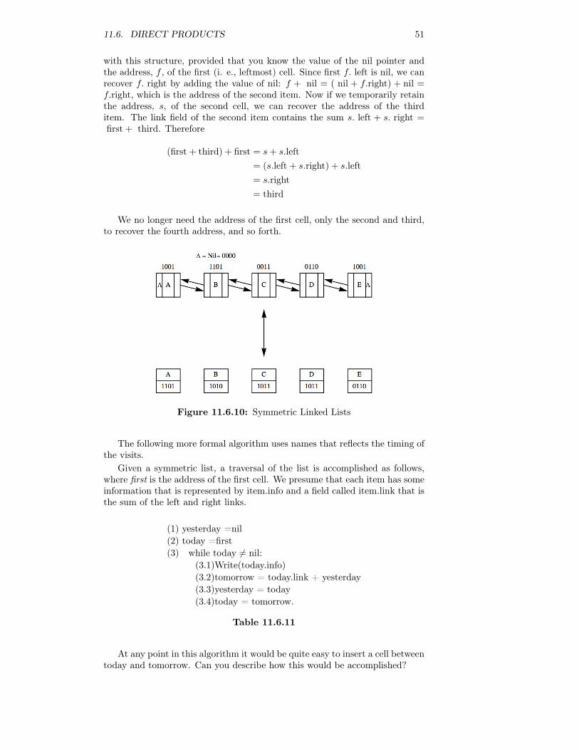
11.6. DIRECT PRODUCTS 51
with this structure, provided that you know the value of the nil pointer andthe address, f , of the first (i. e., leftmost) cell. Since first f. left is nil, we canrecover f. right by adding the value of nil: f + nil = ( nil + f.right) + nil =f.right, which is the address of the second item. Now if we temporarily retainthe address, s, of the second cell, we can recover the address of the thirditem. The link field of the second item contains the sum s. left + s. right =first + third. Therefore
(first + third) + first = s+ s.left= (s.left + s.right) + s.left= s.right= third
We no longer need the address of the first cell, only the second and third,to recover the fourth address, and so forth.
Figure 11.6.10: Symmetric Linked Lists
The following more formal algorithm uses names that reflects the timing ofthe visits.
Given a symmetric list, a traversal of the list is accomplished as follows,where first is the address of the first cell. We presume that each item has someinformation that is represented by item.info and a field called item.link that isthe sum of the left and right links.
(1) yesterday =nil(2) today =first(3) while today 6= nil:
(3.1)Write(today.info)(3.2)tomorrow = today.link + yesterday(3.3)yesterday = today(3.4)today = tomorrow.
Table 11.6.11
At any point in this algorithm it would be quite easy to insert a cell betweentoday and tomorrow. Can you describe how this would be accomplished?
52 CHAPTER 11. ALGEBRAIC STRUCTURES
Exercises for Section 11.6
1. Write out the group table of Z2 × Z3 and find the two proper subgroupsof this group.
2. List more examples of proper subgroups of R2 that are different from theones listed in this section.
3. Algebraic properties of the n-cube.
(a) The four elements of Z22 can be visualized geometrically as the four cor-
ners of the 2-cube. Algebraically describe the statements:
(i) Corners a and b are adjacent.
(ii) Corners a and b are diagonally opposite one another.
(b) The eight elements of Z23 can be visualized as the eight corners of the
3-cube. One face contains Z2 × Z2 × {0} and the opposite face containsthe remaining four elements so that (a, b, 1) is behind (a, b, 0). As in parta, describe statements i and ii algebraically.
(c) If you could imagine a geometric figure similar to the square or cube inn dimensions, and its comers were labeled by elements of Z2
n as in partsa and b, how would statements i and ii be expressed algebraically?
4.
(a) Suppose that you were to be given a group [G; ∗] and asked to solve theequation x ∗ x = e. Without knowing the group, can you anticipate howmany solutions there will be?
(b) Answer the same question as part a for the equation x ∗ x = x.
5. Which of the following sets are subgroups of Z × Z? Give a reason forany negative answers.
(a) {0}
(b) {(2j, 2k) | j, k ∈ Z}
(c) {(2j + 1, 2k) | j, k ∈ Z}
(d) {(n, n2) | n ∈ Z}
(e) {(j, k) | j + k is even}
6. Determine the following values in group Z3 × R∗:
(a) (2, 1) ∗ (1, 2)
(b) the identity element
(c) (1, 1/2)−1
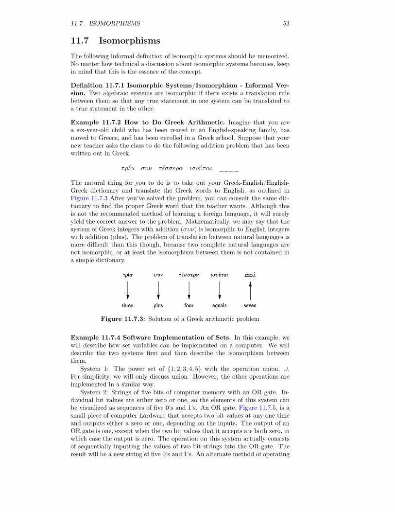
11.7. ISOMORPHISMS 53
11.7 Isomorphisms
The following informal definition of isomorphic systems should be memorized.No matter how technical a discussion about isomorphic systems becomes, keepin mind that this is the essence of the concept.
Definition 11.7.1 Isomorphic Systems/Isomorphism - Informal Ver-sion. Two algebraic systems are isomorphic if there exists a translation rulebetween them so that any true statement in one system can be translated toa true statement in the other.
Example 11.7.2 How to Do Greek Arithmetic. Imagine that you area six-year-old child who has been reared in an English-speaking family, hasmoved to Greece, and has been enrolled in a Greek school. Suppose that yournew teacher asks the class to do the following addition problem that has beenwritten out in Greek.
τρια συν τ εσσερα ισoυται ____
The natural thing for you to do is to take out your Greek-English/English-Greek dictionary and translate the Greek words to English, as outlined inFigure 11.7.3 After you’ve solved the problem, you can consult the same dic-tionary to find the proper Greek word that the teacher wants. Although thisis not the recommended method of learning a foreign language, it will surelyyield the correct answer to the problem. Mathematically, we may say that thesystem of Greek integers with addition (συν) is isomorphic to English integerswith addition (plus). The problem of translation between natural languages ismore difficult than this though, because two complete natural languages arenot isomorphic, or at least the isomorphism between them is not contained ina simple dictionary.
Figure 11.7.3: Solution of a Greek arithmetic problem
Example 11.7.4 Software Implementation of Sets. In this example, wewill describe how set variables can be implemented on a computer. We willdescribe the two systems first and then describe the isomorphism betweenthem.
System 1: The power set of {1, 2, 3, 4, 5} with the operation union, ∪.For simplicity, we will only discuss union. However, the other operations areimplemented in a similar way.
System 2: Strings of five bits of computer memory with an OR gate. In-dividual bit values are either zero or one, so the elements of this system canbe visualized as sequences of five 0’s and 1’s. An OR gate, Figure 11.7.5, is asmall piece of computer hardware that accepts two bit values at any one timeand outputs either a zero or one, depending on the inputs. The output of anOR gate is one, except when the two bit values that it accepts are both zero, inwhich case the output is zero. The operation on this system actually consistsof sequentially inputting the values of two bit strings into the OR gate. Theresult will be a new string of five 0’s and 1’s. An alternate method of operating
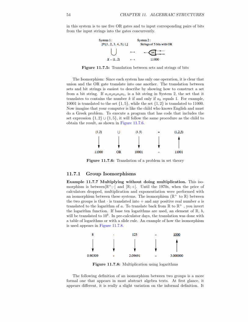
54 CHAPTER 11. ALGEBRAIC STRUCTURES
in this system is to use five OR gates and to input corresponding pairs of bitsfrom the input strings into the gates concurrently.
Figure 11.7.5: Translation between sets and strings of bits
The Isomorphism: Since each system has only one operation, it is clear thatunion and the OR gate translate into one another. The translation betweensets and bit strings is easiest to describe by showing how to construct a setfrom a bit string. If a1a2a3a4a5, is a bit string in System 2, the set that ittranslates to contains the number k if and only if ak equals 1. For example,10001 is translated to the set {1, 5}, while the set {1, 2} is translated to 11000.Now imagine that your computer is like the child who knows English and mustdo a Greek problem. To execute a program that has code that includes theset expression {1, 2} ∪ {1, 5}, it will follow the same procedure as the child toobtain the result, as shown in Figure 11.7.6.
Figure 11.7.6: Translation of a problem in set theory
11.7.1 Group Isomorphisms
Example 11.7.7 Multiplying without doing multiplication. This iso-morphism is between[R+; ·] and [R; +]. Until the 1970s, when the price ofcalculators dropped, multiplication and exponentiation were performed withan isomorphism between these systems. The isomorphism (R+ to R) betweenthe two groups is that · is translated into + and any positive real number a istranslated to the logarithm of a. To translate back from R to R+ , you invertthe logarithm function. If base ten logarithms are used, an element of R, b,will be translated to 10b. In pre-calculator days, the translation was done witha table of logarithms or with a slide rule. An example of how the isomorphismis used appears in Figure 11.7.8.
Figure 11.7.8: Multiplication using logarithms
The following definition of an isomorphism between two groups is a moreformal one that appears in most abstract algebra texts. At first glance, itappears different, it is really a slight variation on the informal definition. It
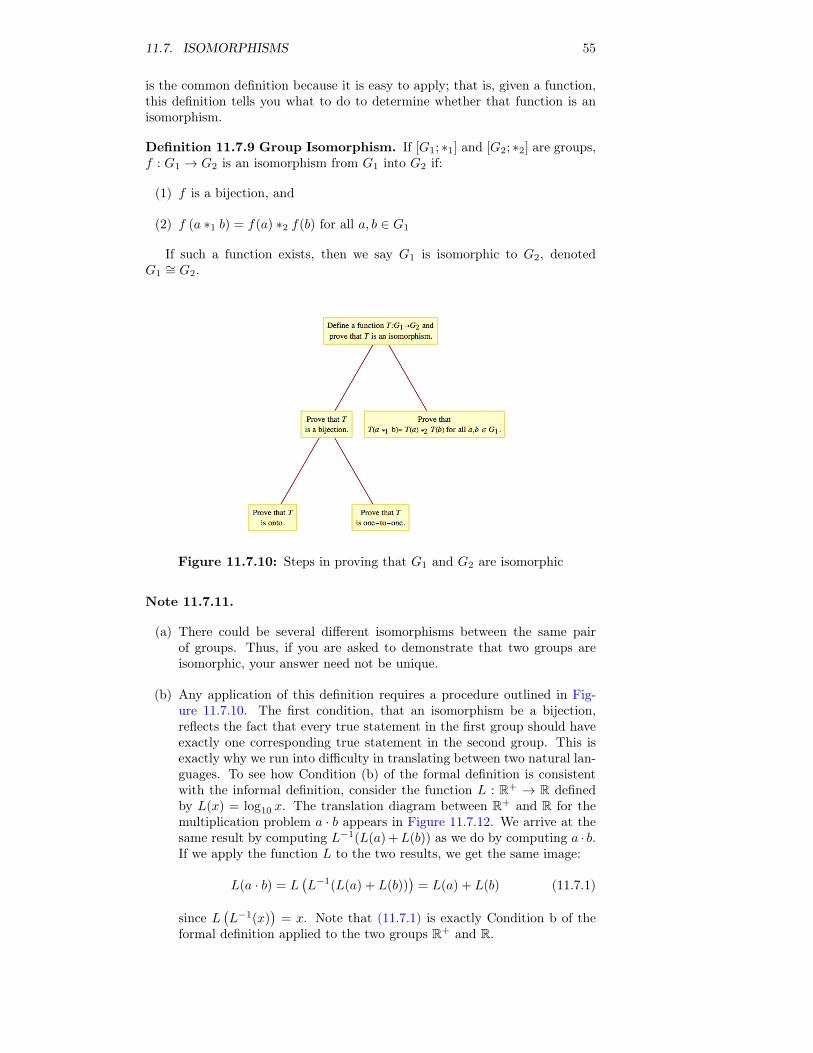
11.7. ISOMORPHISMS 55
is the common definition because it is easy to apply; that is, given a function,this definition tells you what to do to determine whether that function is anisomorphism.
Definition 11.7.9 Group Isomorphism. If [G1; ∗1] and [G2; ∗2] are groups,f : G1 → G2 is an isomorphism from G1 into G2 if:
(1) f is a bijection, and
(2) f (a ∗1 b) = f(a) ∗2 f(b) for all a, b ∈ G1
If such a function exists, then we say G1 is isomorphic to G2, denotedG1∼= G2.
Figure 11.7.10: Steps in proving that G1 and G2 are isomorphic
Note 11.7.11.
(a) There could be several different isomorphisms between the same pairof groups. Thus, if you are asked to demonstrate that two groups areisomorphic, your answer need not be unique.
(b) Any application of this definition requires a procedure outlined in Fig-ure 11.7.10. The first condition, that an isomorphism be a bijection,reflects the fact that every true statement in the first group should haveexactly one corresponding true statement in the second group. This isexactly why we run into difficulty in translating between two natural lan-guages. To see how Condition (b) of the formal definition is consistentwith the informal definition, consider the function L : R+ → R definedby L(x) = log10 x. The translation diagram between R+ and R for themultiplication problem a · b appears in Figure 11.7.12. We arrive at thesame result by computing L−1(L(a) +L(b)) as we do by computing a · b.If we apply the function L to the two results, we get the same image:
L(a · b) = L(L−1(L(a) + L(b))
)= L(a) + L(b) (11.7.1)
since L(L−1(x)
)= x. Note that (11.7.1) is exactly Condition b of the
formal definition applied to the two groups R+ and R.
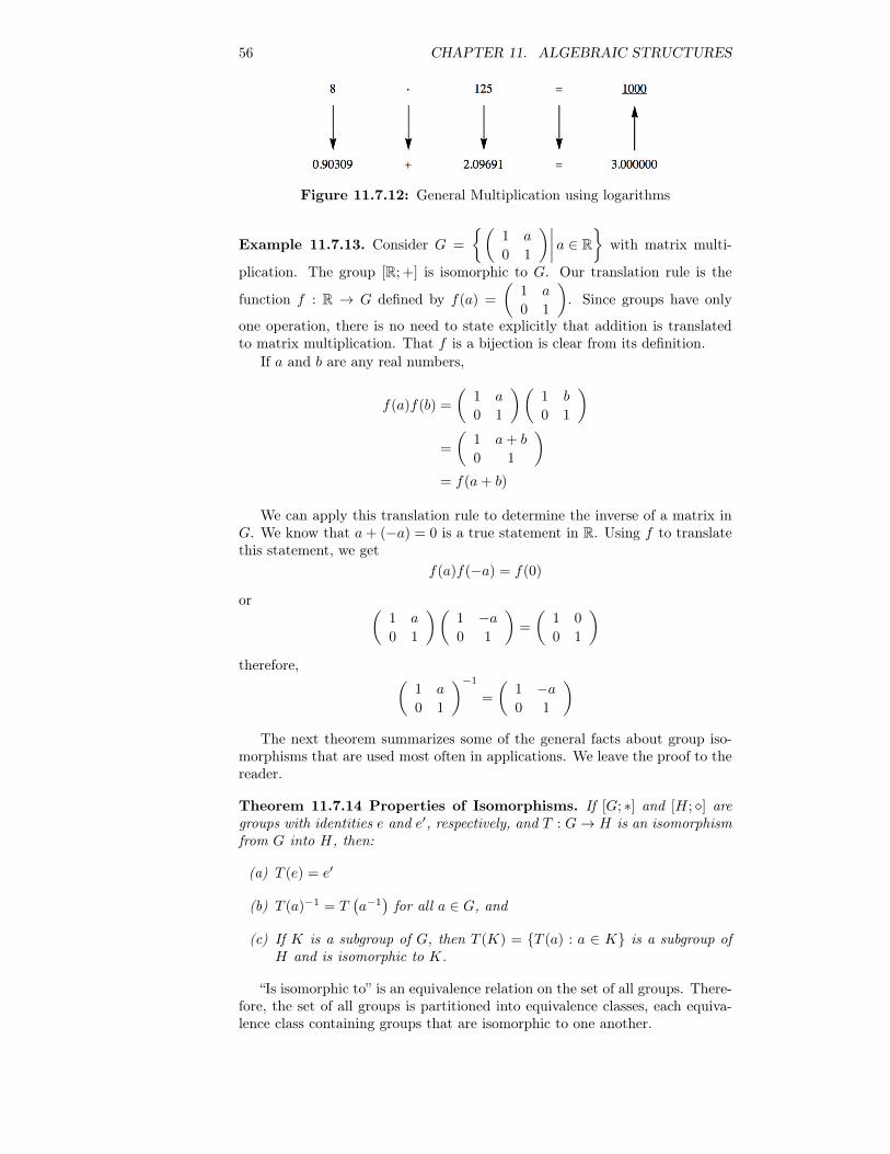
56 CHAPTER 11. ALGEBRAIC STRUCTURES
Figure 11.7.12: General Multiplication using logarithms
Example 11.7.13. Consider G =
{(1 a
0 1
)∣∣∣∣ a ∈ R} with matrix multi-
plication. The group [R; +] is isomorphic to G. Our translation rule is the
function f : R → G defined by f(a) =
(1 a
0 1
). Since groups have only
one operation, there is no need to state explicitly that addition is translatedto matrix multiplication. That f is a bijection is clear from its definition.
If a and b are any real numbers,
f(a)f(b) =
(1 a
0 1
)(1 b
0 1
)=
(1 a+ b
0 1
)= f(a+ b)
We can apply this translation rule to determine the inverse of a matrix inG. We know that a+ (−a) = 0 is a true statement in R. Using f to translatethis statement, we get
f(a)f(−a) = f(0)
or (1 a
0 1
)(1 −a0 1
)=
(1 0
0 1
)therefore, (
1 a
0 1
)−1
=
(1 −a0 1
)The next theorem summarizes some of the general facts about group iso-
morphisms that are used most often in applications. We leave the proof to thereader.
Theorem 11.7.14 Properties of Isomorphisms. If [G; ∗] and [H; �] aregroups with identities e and e′, respectively, and T : G→ H is an isomorphismfrom G into H, then:
(a) T (e) = e′
(b) T (a)−1 = T(a−1
)for all a ∈ G, and
(c) If K is a subgroup of G, then T (K) = {T (a) : a ∈ K} is a subgroup ofH and is isomorphic to K.
“Is isomorphic to” is an equivalence relation on the set of all groups. There-fore, the set of all groups is partitioned into equivalence classes, each equiva-lence class containing groups that are isomorphic to one another.
11.7. ISOMORPHISMS 57
11.7.2 Conditions for groups to not be isomorphicHow do you decide that two groups are not isomorphic to one another? Thenegation of “G and H are isomorphic” is that no translation rule between Gand H exists. If G and H have different cardinalities, then no bijection fromG into H can exist. Hence they are not isomorphic. Given that |G| = |H|, it isusually impractical to list all bijections from G into H and show that none ofthem satisfy Condition b of the formal definition. The best way to prove thattwo groups are not isomorphic is to find a true statement about one group thatis not true about the other group. We illustrate this method in the followingchecklist that you can apply to most pairs of non-isomorphic groups in thisbook.
Assume that [G; ∗] and [H; �] are groups. The following are reasons for Gand H to be not isomorphic.
(a) G and H do not have the same cardinality. For example, Z12 × Z5 can’tbe isomorphic to Z50 and [R; +] can’t be isomorphic to [Q+; ·].
(b) G is abelian and H is not abelian since a ∗ b = b ∗ a is always true inG, but T (a) � T (b) = T (b) � T (a) would not always be true. We haveseen two groups with six elements that apply here. They are Z6 and thegroup of 3 × 3 rook matrices (see Exercise 11.2.5). The second group isnon-abelian, therefore it can’t be isomorphic to Z6.
(c) G has a certain kind of subgroup that H doesn’t have. Part (c) ofTheorem 11.7.14 states that this cannot happen if G is isomorphic toH. [R∗; ·] and [R+; ·] are not isomorphic since R∗ has a subgroup withtwo elements, {−1, 1}, while the proper subgroups of R+ are all infinite(convince yourself of this fact!).
(d) The number of solutions of x ∗ x = e in G is not equal to the number ofsolutions of y � y = e′ in H. Z8 is not isomorphic to Z2
3 since x+8 x = 0has two solutions, 0 and 4, while y + y = (0, 0, 0) is true for all y ∈ Z2
3.If the operation in G is defined by a table, then the number of solutionsof x ∗ x = e will be the number of occurrences of e in the main diagonalof the table. The equations x3 = e, x4 = e, . . . can also be used in thesame way to identify pairs of non-isomorphic groups.
(e) One of the cyclic subgroups of G equals G (i. e., G is cyclic), while noneof H’s cyclic subgroups equals H (i. e., H is noncyclic). This is a specialcase of Condition c. Z and Z × Z are not isomorphic since Z = 〈1〉 andZ× Z is not cyclic.
Exercises for Section 11.71. State whether each pair of groups below is isomorphic. For each pair thatis, give an isomorphism; for those that are not, give your reason.
(a) Z× R and R× Z
(b) Z2 × Z and Z× Z
(c) R and Q×Q
(d) P({1, 2}) with symmetric difference and Z22
(e) Z22 and Z4
(f) R4 and M2×2(R) with matrix addition
58 CHAPTER 11. ALGEBRAIC STRUCTURES
(g) R2 and R× R+
(h) Z2 and the 2× 2 rook matrices
(i) Z6 and Z2 × Z3
2. If you know two natural languages, show that they are not isomorphic.3. Prove that the relation “is isomorphic to” on groups is transitive.4.
(a) Write out the operation table for G = [{1,−1, i,−i}, ·] where i is thecomplex number for which i2 = −1. Show that G is isomorphic to[Z4; +4].
(b) Solve x2 = −1 in G by first translating the equation to Z4 , solving theequation in Z4, and then translating back to G.
5. The two groups [Z4; +4] and [U5;×5] are isomorphic. One isomorphismT : Z4 → U5 is partially defined by T (1) = 3. Determine the values of T (0),T (2), and T (3).6. Prove Theorem 11.7.14.7. Prove that all infinite cyclic groups are isomorphic to Z.8.
(a) Prove that R∗ is isomorphic to Z2 × R.
(b) Describe how multiplication of nonzero real numbers can be accomplisheddoing only additions and translations.
9. Prove that if G is any group and g is some fixed element of G, then thefunction φg defined by φg(x) = g ∗x∗g−1 is an isomorphism from G into itself.An isomorphism of this type is called an inner automorphism.10. It can be shown that there are five non-isomorphic groups of order eight.You should be able to describe at least three of them. Do so without use oftables. Be sure to explain why they are not isomorphic.
Chapter 12
More Matrix Algebra
In Chapter 5 we studied matrix operations and the algebra of sets and logic.We also made note of the strong resemblance of matrix algebra to elementaryalgebra. The reader should briefly review this material. In this chapter weshall look at a powerful matrix tool in the applied sciences, namely a tech-nique for solving systems of linear equations. We will then use this process fordetermining the inverse of n×n matrices, n ≥ 2, when they exist. We proceedwith a development of the diagonalization process, with a discussion of severalof its applications. Finally, we discuss the solution of linear equations over theintegers modulo 2.
12.1 Systems of Linear Equations
12.1.1 Solutions
The method of solving systems of equations by matrices that we will lookat is based on procedures involving equations that we are familiar with fromprevious mathematics courses. The main idea is to reduce a given system ofequations to another simpler system that has the same solutions.
Definition 12.1.1 Solution Set. Given a system of equations involving realvariables x1, x2 . . ., xn, the solution set of the system is the set of n-tuples inRn, (a1, a2, . . . , an) such that the substitutions x1 = a1, x2 = a2, . . ., xn = anmake all the equations true.
In terms of logic, a solution set is a truth set of a system of equations,which is a proposition over n-tuples of real numbers.
In general, if the variables are from a set S, then the solution set willbe a subset of Sn. For example, in number theory mathematicians studyDiophantine equations, where the variables can only take on integer valuesinstead of real values.
Definition 12.1.2 Equivalent Systems of Equations. Two systems of lin-ear equations are called equivalent if they have the same set of solutions.
Example 12.1.3 Two equivalent systems. The previous definition tells usthat if we know that the system
4x1 + 2x2 + x3 = 1
2x1 + x2 + x3 = 4
2x1 + 2x2 + x3 = 3
59
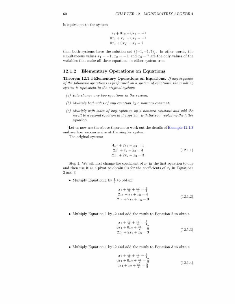
60 CHAPTER 12. MORE MATRIX ALGEBRA
is equivalent to the system
x1 + 0x2 + 0x3 = −1
0x1 + x2 + 0x3 = −1
0x1 + 0x2 + x3 = 7
then both systems have the solution set {(−1,−1, 7)}. In other words, thesimultaneous values x1 = −1, x2 = −1, and x3 = 7 are the only values of thevariables that make all three equations in either system true.
12.1.2 Elementary Operations on EquationsTheorem 12.1.4 Elementary Operations on Equations. If any sequenceof the following operations is performed on a system of equations, the resultingsystem is equivalent to the original system:
(a) Interchange any two equations in the system.
(b) Multiply both sides of any equation by a nonzero constant.
(c) Multiply both sides of any equation by a nonzero constant and add theresult to a second equation in the system, with the sum replacing the latterequation.
Let us now use the above theorem to work out the details of Example 12.1.3and see how we can arrive at the simpler system.
The original system:
4x1 + 2x2 + x3 = 1
2x1 + x2 + x3 = 4
2x1 + 2x2 + x3 = 3
(12.1.1)
Step 1. We will first change the coefficient of x1 in the first equation to oneand then use it as a pivot to obtain 0’s for the coefficients of x1 in Equations2 and 3.
• Multiply Equation 1 by 14 to obtain
x1 + x2
2 + x3
4 = 14
2x1 + x2 + x3 = 4
2x1 + 2x2 + x3 = 3(12.1.2)
• Multiply Equation 1 by -2 and add the result to Equation 2 to obtain
x1 + x2
2 + x3
4 = 14
0x1 + 0x2 + x3
2 = 72
2x1 + 2x2 + x3 = 3(12.1.3)
• Multiply Equation 1 by -2 and add the result to Equation 3 to obtain
x1 + x2
2 + x3
4 = 14
0x1 + 0x2 + x3
2 = 72
0x1 + x2 + x3
2 = 52
(12.1.4)
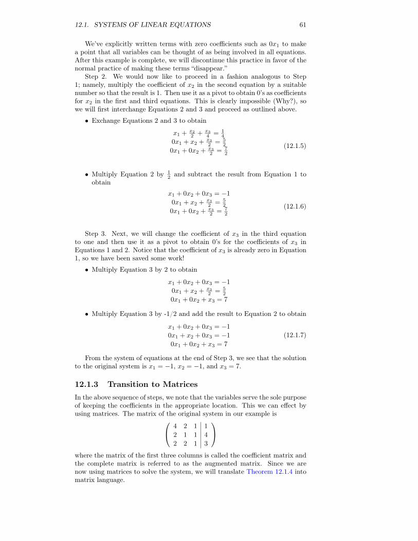
12.1. SYSTEMS OF LINEAR EQUATIONS 61
We’ve explicitly written terms with zero coefficients such as 0x1 to makea point that all variables can be thought of as being involved in all equations.After this example is complete, we will discontinue this practice in favor of thenormal practice of making these terms “disappear.”
Step 2. We would now like to proceed in a fashion analogous to Step1; namely, multiply the coefficient of x2 in the second equation by a suitablenumber so that the result is 1. Then use it as a pivot to obtain 0’s as coefficientsfor x2 in the first and third equations. This is clearly impossible (Why?), sowe will first interchange Equations 2 and 3 and proceed as outlined above.
• Exchange Equations 2 and 3 to obtain
x1 + x2
2 + x3
4 = 14
0x1 + x2 + x3
2 = 52
0x1 + 0x2 + x3
2 = 72
(12.1.5)
• Multiply Equation 2 by 12 and subtract the result from Equation 1 to
obtain
x1 + 0x2 + 0x3 = −1
0x1 + x2 + x3
2 = 52
0x1 + 0x2 + x3
2 = 72
(12.1.6)
Step 3. Next, we will change the coefficient of x3 in the third equationto one and then use it as a pivot to obtain 0’s for the coefficients of x3 inEquations 1 and 2. Notice that the coefficient of x3 is already zero in Equation1, so we have been saved some work!
• Multiply Equation 3 by 2 to obtain
x1 + 0x2 + 0x3 = −1
0x1 + x2 + x3
2 = 52
0x1 + 0x2 + x3 = 7
• Multiply Equation 3 by -1/2 and add the result to Equation 2 to obtain
x1 + 0x2 + 0x3 = −1
0x1 + x2 + 0x3 = −1
0x1 + 0x2 + x3 = 7
(12.1.7)
From the system of equations at the end of Step 3, we see that the solutionto the original system is x1 = −1, x2 = −1, and x3 = 7.
12.1.3 Transition to MatricesIn the above sequence of steps, we note that the variables serve the sole purposeof keeping the coefficients in the appropriate location. This we can effect byusing matrices. The matrix of the original system in our example is 4 2 1 1
2 1 1 4
2 2 1 3
where the matrix of the first three columns is called the coefficient matrix andthe complete matrix is referred to as the augmented matrix. Since we arenow using matrices to solve the system, we will translate Theorem 12.1.4 intomatrix language.
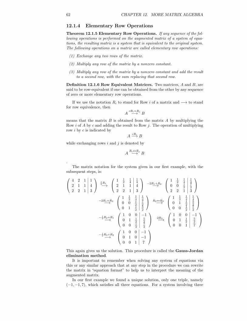
62 CHAPTER 12. MORE MATRIX ALGEBRA
12.1.4 Elementary Row OperationsTheorem 12.1.5 Elementary Row Operations. If any sequence of the fol-lowing operations is performed on the augmented matrix of a system of equa-tions, the resulting matrix is a system that is equivalent to the original system.The following operations on a matrix are called elementary row operations:
(1) Exchange any two rows of the matrix.
(2) Multiply any row of the matrix by a nonzero constant.
(3) Multiply any row of the matrix by a nonzero constant and add the resultto a second row, with the sum replacing that second row.
Definition 12.1.6 Row Equivalent Matrices. Two matrices, A and B, aresaid to be row-equivalent if one can be obtained from the other by any sequenceof zero or more elementary row operations.
If we use the notation Ri to stand for Row i of a matrix and −→ to standfor row equivalence, then
AcRi+Rj−→ B
means that the matrix B is obtained from the matrix A by multiplying theRow i of A by c and adding the result to Row j. The operation of multiplyingrow i by c is indicated by
AcRi−→ B
while exchanging rows i and j is denoted by
ARi↔Rj−→ B
.The matrix notation for the system given in our first example, with the
subsequent steps, is: 4 2 1 1
2 1 1 4
2 2 1 3
14R1−→
1 12
14
14
2 1 1 4
2 2 1 3
−2R1+R2−→
1 12
14
14
0 0 12
72
2 2 1 3
−2R1+R3−→
1 12
14
14
0 0 12
72
0 1 12
52
R2↔R3−→
1 12
14
14
0 1 12
52
0 0 12
72
− 1
2R2+R1−→
1 0 0 −1
0 1 12
52
0 0 12
72
2R3−→
1 0 0 −1
0 1 12
52
0 0 1 7
− 1
2R3+R2−→
1 0 0 −1
0 1 0 −1
0 0 1 7
This again gives us the solution. This procedure is called the Gauss-Jordanelimination method.
It is important to remember when solving any system of equations viathis or any similar approach that at any step in the procedure we can rewritethe matrix in “equation format” to help us to interpret the meaning of theaugmented matrix.
In our first example we found a unique solution, only one triple, namely(−1,−1, 7), which satisfies all three equations. For a system involving three
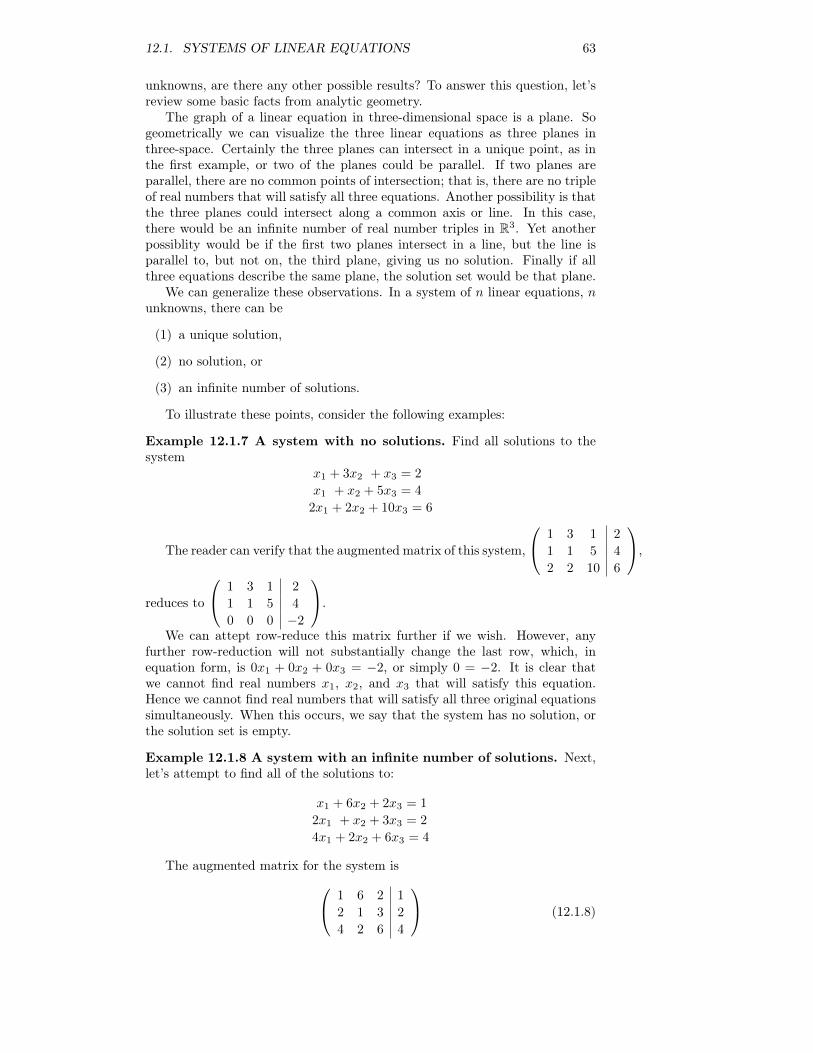
12.1. SYSTEMS OF LINEAR EQUATIONS 63
unknowns, are there any other possible results? To answer this question, let’sreview some basic facts from analytic geometry.
The graph of a linear equation in three-dimensional space is a plane. Sogeometrically we can visualize the three linear equations as three planes inthree-space. Certainly the three planes can intersect in a unique point, as inthe first example, or two of the planes could be parallel. If two planes areparallel, there are no common points of intersection; that is, there are no tripleof real numbers that will satisfy all three equations. Another possibility is thatthe three planes could intersect along a common axis or line. In this case,there would be an infinite number of real number triples in R3. Yet anotherpossiblity would be if the first two planes intersect in a line, but the line isparallel to, but not on, the third plane, giving us no solution. Finally if allthree equations describe the same plane, the solution set would be that plane.
We can generalize these observations. In a system of n linear equations, nunknowns, there can be
(1) a unique solution,
(2) no solution, or
(3) an infinite number of solutions.
To illustrate these points, consider the following examples:
Example 12.1.7 A system with no solutions. Find all solutions to thesystem
x1 + 3x2 + x3 = 2
x1 + x2 + 5x3 = 4
2x1 + 2x2 + 10x3 = 6
The reader can verify that the augmented matrix of this system,
1 3 1 2
1 1 5 4
2 2 10 6
,
reduces to
1 3 1 2
1 1 5 4
0 0 0 −2
.
We can attept row-reduce this matrix further if we wish. However, anyfurther row-reduction will not substantially change the last row, which, inequation form, is 0x1 + 0x2 + 0x3 = −2, or simply 0 = −2. It is clear thatwe cannot find real numbers x1, x2, and x3 that will satisfy this equation.Hence we cannot find real numbers that will satisfy all three original equationssimultaneously. When this occurs, we say that the system has no solution, orthe solution set is empty.
Example 12.1.8 A system with an infinite number of solutions. Next,let’s attempt to find all of the solutions to:
x1 + 6x2 + 2x3 = 1
2x1 + x2 + 3x3 = 2
4x1 + 2x2 + 6x3 = 4
The augmented matrix for the system is 1 6 2 1
2 1 3 2
4 2 6 4
(12.1.8)
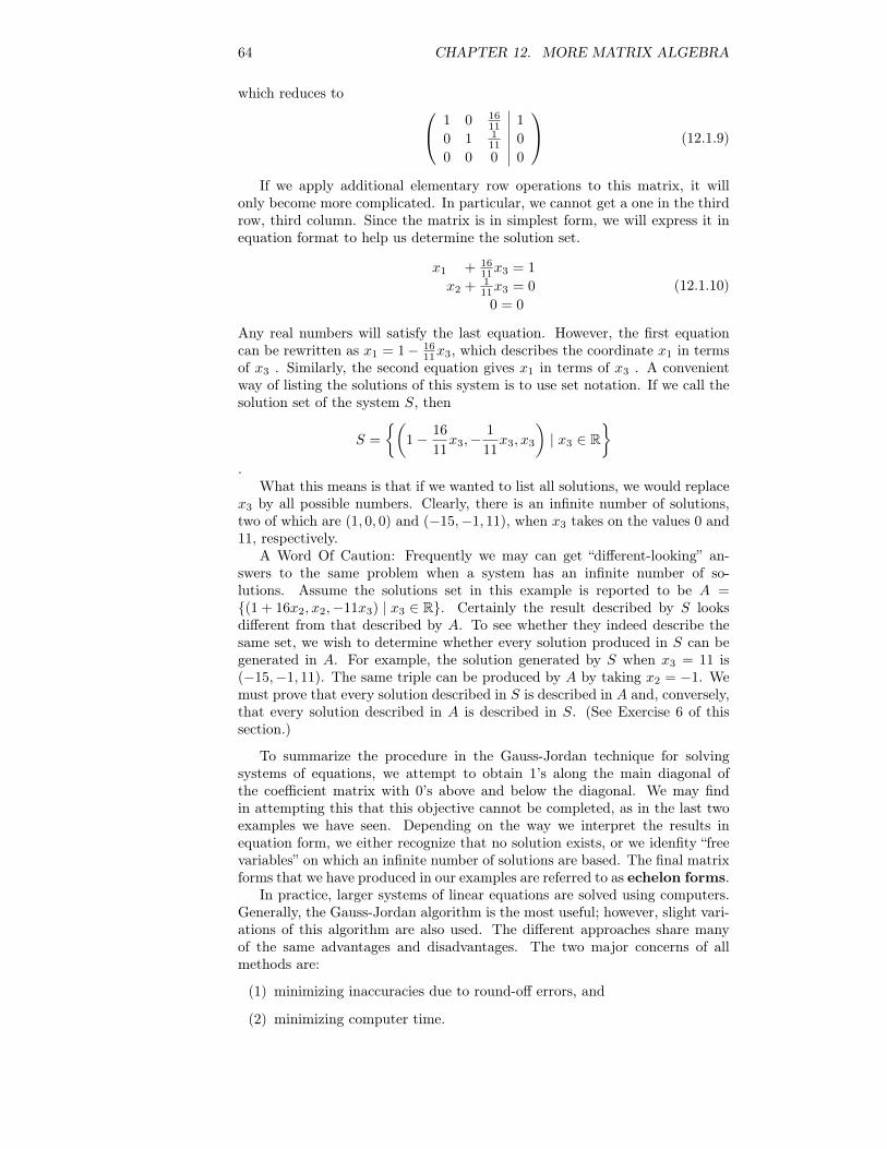
64 CHAPTER 12. MORE MATRIX ALGEBRA
which reduces to 1 0 1611 1
0 1 111 0
0 0 0 0
(12.1.9)
If we apply additional elementary row operations to this matrix, it willonly become more complicated. In particular, we cannot get a one in the thirdrow, third column. Since the matrix is in simplest form, we will express it inequation format to help us determine the solution set.
x1 + 1611x3 = 1
x2 + 111x3 = 0
0 = 0
(12.1.10)
Any real numbers will satisfy the last equation. However, the first equationcan be rewritten as x1 = 1− 16
11x3, which describes the coordinate x1 in termsof x3 . Similarly, the second equation gives x1 in terms of x3 . A convenientway of listing the solutions of this system is to use set notation. If we call thesolution set of the system S, then
S =
{(1− 16
11x3,−
1
11x3, x3
)| x3 ∈ R
}.
What this means is that if we wanted to list all solutions, we would replacex3 by all possible numbers. Clearly, there is an infinite number of solutions,two of which are (1, 0, 0) and (−15,−1, 11), when x3 takes on the values 0 and11, respectively.
A Word Of Caution: Frequently we may can get “different-looking” an-swers to the same problem when a system has an infinite number of so-lutions. Assume the solutions set in this example is reported to be A ={(1 + 16x2, x2,−11x3) | x3 ∈ R}. Certainly the result described by S looksdifferent from that described by A. To see whether they indeed describe thesame set, we wish to determine whether every solution produced in S can begenerated in A. For example, the solution generated by S when x3 = 11 is(−15,−1, 11). The same triple can be produced by A by taking x2 = −1. Wemust prove that every solution described in S is described in A and, conversely,that every solution described in A is described in S. (See Exercise 6 of thissection.)
To summarize the procedure in the Gauss-Jordan technique for solvingsystems of equations, we attempt to obtain 1’s along the main diagonal ofthe coefficient matrix with 0’s above and below the diagonal. We may findin attempting this that this objective cannot be completed, as in the last twoexamples we have seen. Depending on the way we interpret the results inequation form, we either recognize that no solution exists, or we idenfity “freevariables” on which an infinite number of solutions are based. The final matrixforms that we have produced in our examples are referred to as echelon forms.
In practice, larger systems of linear equations are solved using computers.Generally, the Gauss-Jordan algorithm is the most useful; however, slight vari-ations of this algorithm are also used. The different approaches share manyof the same advantages and disadvantages. The two major concerns of allmethods are:
(1) minimizing inaccuracies due to round-off errors, and
(2) minimizing computer time.
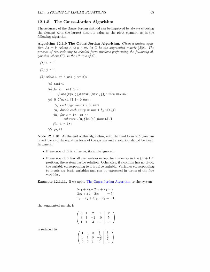
12.1. SYSTEMS OF LINEAR EQUATIONS 65
12.1.5 The Gauss-Jordan AlgorithmThe accuracy of the Gauss-Jordan method can be improved by always choosingthe element with the largest absolute value as the pivot element, as in thefollowing algorithm.
Algorithm 12.1.9 The Gauss-Jordan Algorithm. Given a matrix equa-tion Ax = b, where A is n × m, let C be the augmented matrix [A|b]. Theprocess of row-reducing to echelon form involves performing the following al-gorithm where C[i] is the ith row of C.
(1) i = 1
(2) j = 1
(3) while i <= n and j <= m):
(a) maxi=i
(b) for k = i+1 to n:if abs(C[k,j])>abs(C[maxi,j]): then maxi=k
(c) if C[maxi,j] != 0 then:
(i) exchange rows i and maxi
(ii) divide each entry in row i by C[i,j]
(iii) for u = i+1 to n:subtract C[u,j]*C[i] from C[u]
(iv) i = i+1
(d) j=j+1
Note 12.1.10. At the end of this algorithm, with the final form of C you canrevert back to the equation form of the system and a solution should be clear.In general,
• If any row of C is all zeros, it can be ignored.
• If any row of C has all zero entries except for the entry in the (m+ 1)st
position, the system has no solution. Otherwise, if a column has no pivot,the variable corresponding to it is a free variable. Variables correspondingto pivots are basic variables and can be expressed in terms of the freevariables.
Example 12.1.11. If we apply The Gauss-Jordan Algorithm to the system
5x1 + x2 + 2x3 + x4 = 2
3x1 + x2 − 2x3 = 5
x1 + x2 + 3x3 − x4 = −1
the augmented matrix is 5 1 2 1 2
3 1 −2 0 5
1 1 3 −1 −1
is reduced to 1 0 0 1
212
0 1 0 − 32
32
0 0 1 0 −1
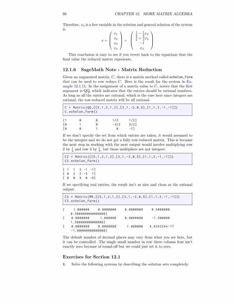
66 CHAPTER 12. MORE MATRIX ALGEBRA
Therefore, x4 is a free variable in the solution and general solution of the systemis
x =
x1
x2
x3
x4
=
12 −
12x4
32 + 3
2x4
−1
x4
This conclusion is easy to see if you revert back to the equations that the
final value the reduced matrix represents.
12.1.6 SageMath Note - Matrix ReductionGiven an augmented matrix, C, there is a matrix method called echelon_formthat can be used to row reduce C. Here is the result for the system in Ex-ample 12.1.11. In the assignment of a matrix value to C, notice that the firstargument is QQ, which indicates that the entries should be rational numbers.As long as all the entries are rational, which is the case here since integers arerational, the row-reduced matrix will be all rational.
C = Matrix(QQ ,[[5,1,2,1,2],[3,1,-2,0,5],[1,1,3,-1,-1]])C.echelon_form ()
[1 0 0 1/2 1/2][0 1 0 -3/2 3/2][0 0 1 0 -1]
If we don’t specify the set from which entries are taken, it would assumed tobe the integers and we do not get a fully row-reduced matrix. This is becausethe next step in working with the next output would involve multiplying row2 by 1
2 and row 3 by 19 , but these multipliers are not integers.
C2 = Matrix ([[5,1,2,1,2],[3,1,-2,0,5],[1,1,3,-1,-1]])C2.echelon_form ()
[ 1 1 3 -1 -1][ 0 2 2 -3 1][ 0 0 9 0 -9]
If we specifying real entries, the result isn’t as nice and clean as the rationaloutput.
C3 = Matrix(RR ,[[5,1,2,1,2],[3,1,-2,0,5],[1,1,3,-1,-1]])C3.echelon_form ()
[ 1.000000 0.0000000 0.0000000 0.50000000.500000000000000]
[ 0.0000000 1.000000 0.0000000 -1.5000001.50000000000000]
[ 0.0000000 0.0000000 1.000000 4.934324e-17-1.00000000000000]
The default number of decimal places may vary from what you see here, butit can be controlled. The single small number in row three column four isn’texactly zero because of round-off but we could just set it to zero.
Exercises for Section 12.11. Solve the following systems by describing the solution sets completely:
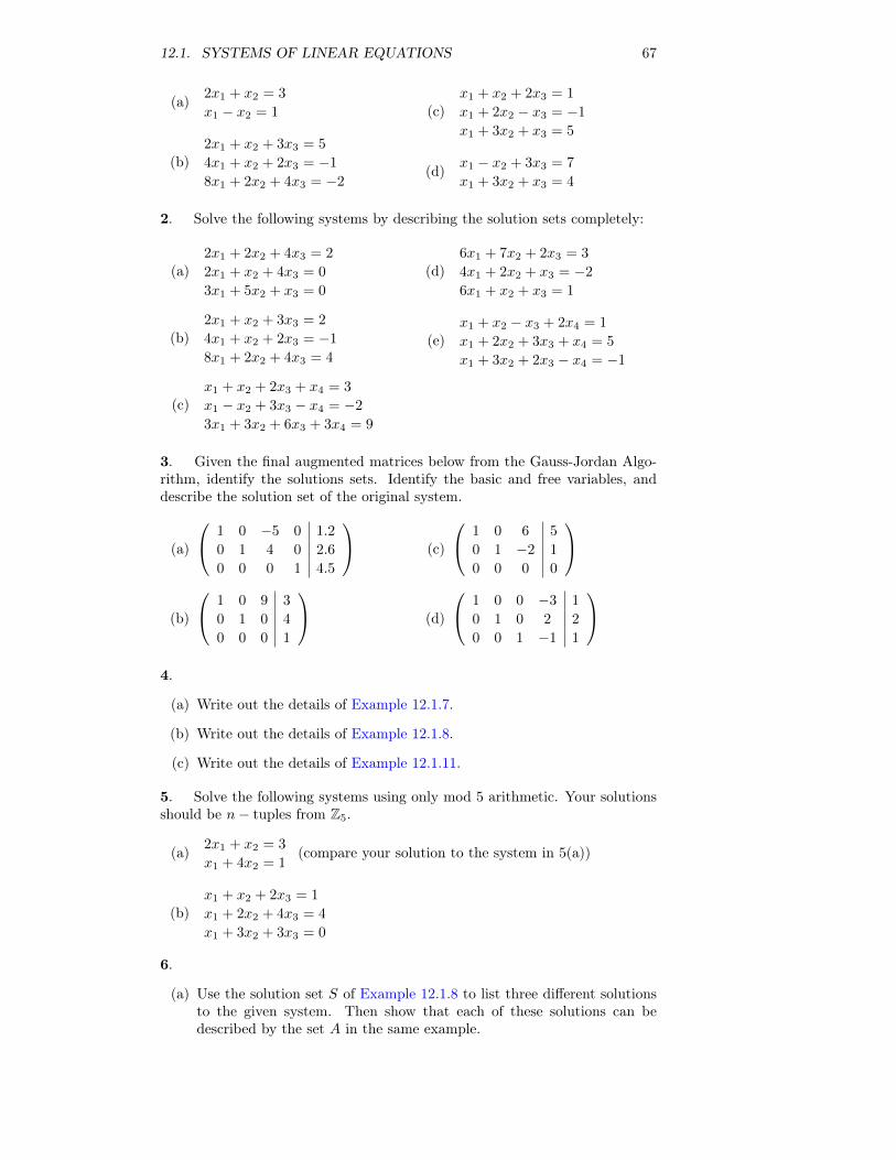
12.1. SYSTEMS OF LINEAR EQUATIONS 67
(a) 2x1 + x2 = 3
x1 − x2 = 1
(b)2x1 + x2 + 3x3 = 5
4x1 + x2 + 2x3 = −1
8x1 + 2x2 + 4x3 = −2
(c)x1 + x2 + 2x3 = 1
x1 + 2x2 − x3 = −1
x1 + 3x2 + x3 = 5
(d) x1 − x2 + 3x3 = 7
x1 + 3x2 + x3 = 4
2. Solve the following systems by describing the solution sets completely:
(a)2x1 + 2x2 + 4x3 = 2
2x1 + x2 + 4x3 = 0
3x1 + 5x2 + x3 = 0
(b)2x1 + x2 + 3x3 = 2
4x1 + x2 + 2x3 = −1
8x1 + 2x2 + 4x3 = 4
(c)x1 + x2 + 2x3 + x4 = 3
x1 − x2 + 3x3 − x4 = −2
3x1 + 3x2 + 6x3 + 3x4 = 9
(d)6x1 + 7x2 + 2x3 = 3
4x1 + 2x2 + x3 = −2
6x1 + x2 + x3 = 1
(e)x1 + x2 − x3 + 2x4 = 1
x1 + 2x2 + 3x3 + x4 = 5
x1 + 3x2 + 2x3 − x4 = −1
3. Given the final augmented matrices below from the Gauss-Jordan Algo-rithm, identify the solutions sets. Identify the basic and free variables, anddescribe the solution set of the original system.
(a)
1 0 −5 0 1.2
0 1 4 0 2.6
0 0 0 1 4.5
(b)
1 0 9 3
0 1 0 4
0 0 0 1
(c)
1 0 6 5
0 1 −2 1
0 0 0 0
(d)
1 0 0 −3 1
0 1 0 2 2
0 0 1 −1 1
4.
(a) Write out the details of Example 12.1.7.
(b) Write out the details of Example 12.1.8.
(c) Write out the details of Example 12.1.11.
5. Solve the following systems using only mod 5 arithmetic. Your solutionsshould be n− tuples from Z5.
(a) 2x1 + x2 = 3
x1 + 4x2 = 1(compare your solution to the system in 5(a))
(b)x1 + x2 + 2x3 = 1
x1 + 2x2 + 4x3 = 4
x1 + 3x2 + 3x3 = 0
6.
(a) Use the solution set S of Example 12.1.8 to list three different solutionsto the given system. Then show that each of these solutions can bedescribed by the set A in the same example.
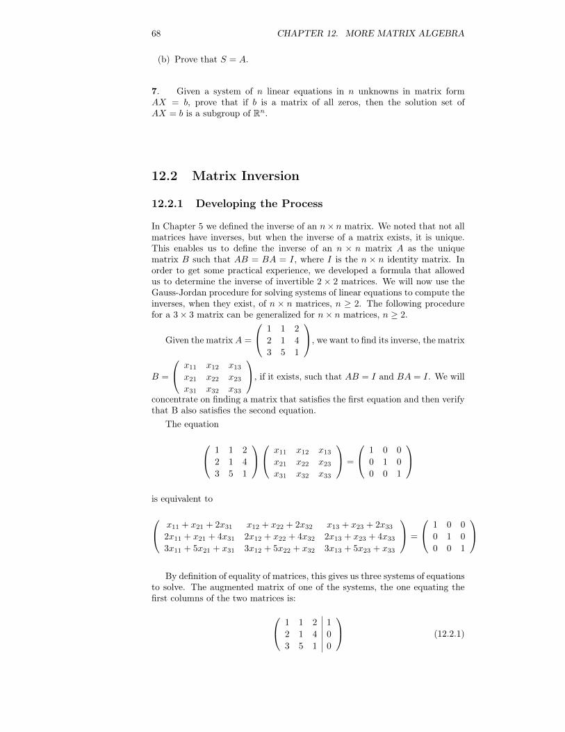
68 CHAPTER 12. MORE MATRIX ALGEBRA
(b) Prove that S = A.
7. Given a system of n linear equations in n unknowns in matrix formAX = b, prove that if b is a matrix of all zeros, then the solution set ofAX = b is a subgroup of Rn.
12.2 Matrix Inversion
12.2.1 Developing the Process
In Chapter 5 we defined the inverse of an n× n matrix. We noted that not allmatrices have inverses, but when the inverse of a matrix exists, it is unique.This enables us to define the inverse of an n × n matrix A as the uniquematrix B such that AB = BA = I, where I is the n × n identity matrix. Inorder to get some practical experience, we developed a formula that allowedus to determine the inverse of invertible 2 × 2 matrices. We will now use theGauss-Jordan procedure for solving systems of linear equations to compute theinverses, when they exist, of n × n matrices, n ≥ 2. The following procedurefor a 3× 3 matrix can be generalized for n× n matrices, n ≥ 2.
Given the matrix A =
1 1 2
2 1 4
3 5 1
, we want to find its inverse, the matrix
B =
x11 x12 x13
x21 x22 x23
x31 x32 x33
, if it exists, such that AB = I and BA = I. We will
concentrate on finding a matrix that satisfies the first equation and then verifythat B also satisfies the second equation.
The equation
1 1 2
2 1 4
3 5 1
x11 x12 x13
x21 x22 x23
x31 x32 x33
=
1 0 0
0 1 0
0 0 1
is equivalent to
x11 + x21 + 2x31 x12 + x22 + 2x32 x13 + x23 + 2x33
2x11 + x21 + 4x31 2x12 + x22 + 4x32 2x13 + x23 + 4x33
3x11 + 5x21 + x31 3x12 + 5x22 + x32 3x13 + 5x23 + x33
=
1 0 0
0 1 0
0 0 1
By definition of equality of matrices, this gives us three systems of equations
to solve. The augmented matrix of one of the systems, the one equating thefirst columns of the two matrices is: 1 1 2 1
2 1 4 0
3 5 1 0
(12.2.1)
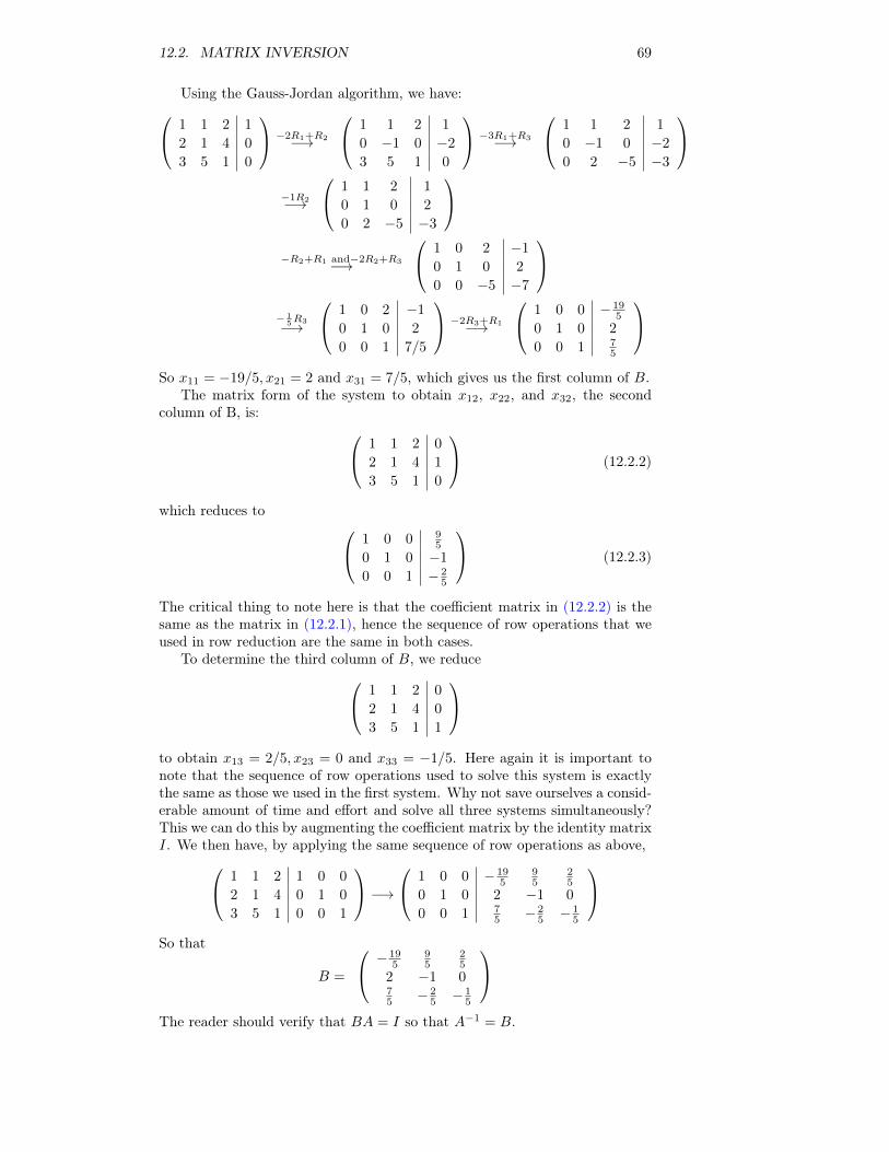
12.2. MATRIX INVERSION 69
Using the Gauss-Jordan algorithm, we have: 1 1 2 1
2 1 4 0
3 5 1 0
−2R1+R2−→
1 1 2 1
0 −1 0 −2
3 5 1 0
−3R1+R3−→
1 1 2 1
0 −1 0 −2
0 2 −5 −3
−1R2−→
1 1 2 1
0 1 0 2
0 2 −5 −3
−R2+R1 and−2R2+R3−→
1 0 2 −1
0 1 0 2
0 0 −5 −7
− 1
5R3−→
1 0 2 −1
0 1 0 2
0 0 1 7/5
−2R3+R1−→
1 0 0 − 195
0 1 0 2
0 0 1 75
So x11 = −19/5, x21 = 2 and x31 = 7/5, which gives us the first column of B.
The matrix form of the system to obtain x12, x22, and x32, the secondcolumn of B, is: 1 1 2 0
2 1 4 1
3 5 1 0
(12.2.2)
which reduces to 1 0 0 95
0 1 0 −1
0 0 1 − 25
(12.2.3)
The critical thing to note here is that the coefficient matrix in (12.2.2) is thesame as the matrix in (12.2.1), hence the sequence of row operations that weused in row reduction are the same in both cases.
To determine the third column of B, we reduce 1 1 2 0
2 1 4 0
3 5 1 1
to obtain x13 = 2/5, x23 = 0 and x33 = −1/5. Here again it is important tonote that the sequence of row operations used to solve this system is exactlythe same as those we used in the first system. Why not save ourselves a consid-erable amount of time and effort and solve all three systems simultaneously?This we can do this by augmenting the coefficient matrix by the identity matrixI. We then have, by applying the same sequence of row operations as above, 1 1 2 1 0 0
2 1 4 0 1 0
3 5 1 0 0 1
−→ 1 0 0 − 19
595
25
0 1 0 2 −1 0
0 0 1 75 − 2
5 − 15
So that
B =
− 195
95
25
2 −1 075 − 2
5 − 15
The reader should verify that BA = I so that A−1 = B.
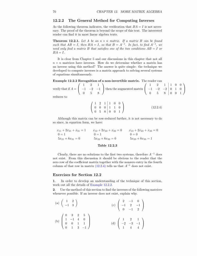
70 CHAPTER 12. MORE MATRIX ALGEBRA
12.2.2 The General Method for Computing InversesAs the following theorem indicates, the verification that BA = I is not neces-sary. The proof of the theorem is beyond the scope of this text. The interestedreader can find it in most linear algebra texts.
Theorem 12.2.1. Let A be an n × n matrix. If a matrix B can be foundsuch that AB = I, then BA = I, so that B = A−1. In fact, to find A−1, weneed only find a matrix B that satisfies one of the two conditions AB = I orBA = I.
It is clear from Chapter 5 and our discussions in this chapter that not alln × n matrices have inverses. How do we determine whether a matrix hasan inverse using this method? The answer is quite simple: the technique wedeveloped to compute inverses is a matrix approach to solving several systemsof equations simultaneously.
Example 12.2.2 Recognition of a non-invertible matrix. The reader can
verify that ifA =
1 2 1
−1 −2 −1
0 5 8
then the augmented matrix
1 2 1 1 0 0
−1 −2 −2 0 1 0
0 5 8 0 0 1
reduces to 1 2 1 1 0 0
0 0 0 1 1 0
0 5 8 0 0 1
(12.2.4)
Although this matrix can be row-reduced further, it is not necessary to doso since, in equation form, we have:
x11 + 2x21 + x31 = 1
0 = 1
5x21 + 8x31 = 0
x12 + 2x22 + x32 = 0
0 = 1
5x22 + 8x32 = 0
x13 + 2x23 + x33 = 0
0 = 0
5x23 + 8x33 = 1
Table 12.2.3
Clearly, there are no solutions to the first two systems, therefore A−1 doesnot exist. From this discussion it should be obvious to the reader that thezero row of the coefficient matrix together with the nonzero entry in the fourthcolumn of that row in matrix (12.2.4) tells us that A−1 does not exist.
Exercises for Section 12.21. In order to develop an understanding of the technique of this section,work out all the details of Example 12.2.2.2. Use the method of this section to find the inverses of the following matriceswhenever possible. If an inverse does not exist, explain why.
(a)(
1 2
−1 3
)
(b)
0 3 2 5
1 −1 4 0
0 0 1 1
0 1 3 −1
(c)
2 −1 0
−1 2 −1
0 −1 2
(d)
1 2 1
−2 −3 −1
1 4 4
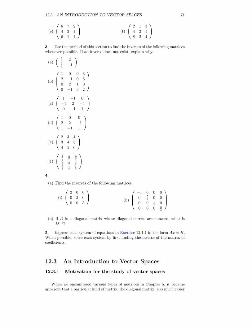
12.3. AN INTRODUCTION TO VECTOR SPACES 71
(e)
6 7 2
4 2 1
6 1 1
(f)
2 1 3
4 2 1
8 2 4
3. Use the method of this section to find the inverses of the following matriceswhenever possible. If an inverse does not exist, explain why.
(a)(
13 215 −1
)
(b)
1 0 0 3
2 −1 0 6
0 2 1 0
0 −1 3 2
(c)
1 −1 0
−1 2 −1
0 −1 1
(d)
1 0 0
2 2 −1
1 −1 1
(e)
2 3 4
3 4 5
4 5 6
(f)
1 12
13
12
13
14
13
14
15
4.
(a) Find the inverses of the following matrices.
(i)
2 0 0
0 3 0
0 0 5
(ii)
−1 0 0 0
0 52 0 0
0 0 17 0
0 0 0 34
(b) If D is a diagonal matrix whose diagonal entries are nonzero, what is
D−1?
5. Express each system of equations in Exercise 12.1.1 in the form Ax = B.When possible, solve each system by first finding the inverse of the matrix ofcoefficients.
12.3 An Introduction to Vector Spaces
12.3.1 Motivation for the study of vector spaces
When we encountered various types of matrices in Chapter 5, it becameapparent that a particular kind of matrix, the diagonal matrix, was much easier
72 CHAPTER 12. MORE MATRIX ALGEBRA
to use in computations. For example, if A =
(2 1
2 3
), then A5 can be found,
but its computation is tedious. If D =
(1 0
0 4
)then
D5 =
(1 0
0 4
)5
=
(15 0
0 45
)=
(1 0
0 1024
)Even when presented with a non-diagonal matrix, we will see that it is some-times possible to do a bit of work to be able to work with a diagonal matrix.This process is called diagonalization.
In a variety of applications it is beneficial to be able to diagonalize a ma-trix. In this section we will investigate what this means and consider a fewapplications. In order to understand when the diagonalization process canbe performed, it is necessary to develop several of the underlying concepts oflinear algebra.
12.3.2 Vector SpacesBy now, you realize that mathematicians tend to generalize. Once we havefound a “good thing,” something that is useful, we apply it to as many dif-ferent concepts as possible. In doing so, we frequently find that the “differentconcepts” are not really different but only look different. Four sentences in fourdifferent languages might look dissimilar, but when they are translated into acommon language, they might very well express the exact same idea.
Early in the development of mathematics, the concept of a vector led toa variety of applications in physics and engineering. We can certainly picturevectors, or “arrows,” in the xy − plane and even in the three-dimensionalspace. Does it make sense to talk about vectors in four-dimensional space, inten-dimensional space, or in any other mathematical situation? If so, what isthe essence of a vector? Is it its shape or the rules it follows? The shape intwo- or three-space is just a picture, or geometric interpretation, of a vector.The essence is the rules, or properties, we wish vectors to follow so we canmanipulate them algebraically. What follows is a definition of what is called avector space. It is a list of all the essential properties of vectors, and it is thebasic definition of the branch of mathematics called linear algebra.
Definition 12.3.1 Vector Space. Let V be any nonempty set of objects.Define on V an operation, called addition, for any two elements x,y ∈ V , anddenote this operation by x + y. Let scalar multiplication be defined for a realnumber a ∈ R and any element x ∈ V and denote this operation by ax. Theset V together with operations of addition and scalar multiplication is calleda vector space over R if the following hold for all x,y, z ∈ V , and a, b ∈ R:
• x + y = y + x
• (x + y) + z = x + (y + z)
• There exists a vector 0 ∈ V , such that x + 0 = x for all x ∈ V .
• For each vector x ∈ V , there exists a unique vector −x ∈ V , such that−x + x = 0.
These are the main properties associated with the operation of addition. Theycan be summarized by saying that [V ; +] is an abelian group.
The next four properties are associated with the operation of scalar multi-plication and how it relates to vector addition.
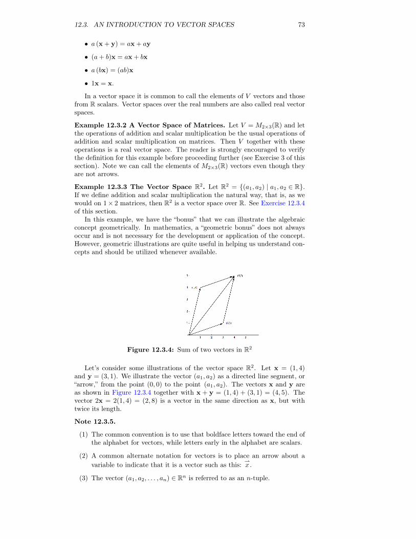
12.3. AN INTRODUCTION TO VECTOR SPACES 73
• a (x + y) = ax + ay
• (a+ b)x = ax + bx
• a (bx) = (ab)x
• 1x = x.
In a vector space it is common to call the elements of V vectors and thosefrom R scalars. Vector spaces over the real numbers are also called real vectorspaces.
Example 12.3.2 A Vector Space of Matrices. Let V = M2×3(R) and letthe operations of addition and scalar multiplication be the usual operations ofaddition and scalar multiplication on matrices. Then V together with theseoperations is a real vector space. The reader is strongly encouraged to verifythe definition for this example before proceeding further (see Exercise 3 of thissection). Note we can call the elements of M2×3(R) vectors even though theyare not arrows.
Example 12.3.3 The Vector Space R2. Let R2 = {(a1, a2) | a1, a2 ∈ R}.If we define addition and scalar multiplication the natural way, that is, as wewould on 1× 2 matrices, then R2 is a vector space over R. See Exercise 12.3.4of this section.
In this example, we have the “bonus” that we can illustrate the algebraicconcept geometrically. In mathematics, a “geometric bonus” does not alwaysoccur and is not necessary for the development or application of the concept.However, geometric illustrations are quite useful in helping us understand con-cepts and should be utilized whenever available.
Figure 12.3.4: Sum of two vectors in R2
Let’s consider some illustrations of the vector space R2. Let x = (1, 4)and y = (3, 1). We illustrate the vector (a1, a2) as a directed line segment, or“arrow,” from the point (0, 0) to the point (a1, a2). The vectors x and y areas shown in Figure 12.3.4 together with x + y = (1, 4) + (3, 1) = (4, 5). Thevector 2x = 2(1, 4) = (2, 8) is a vector in the same direction as x, but withtwice its length.
Note 12.3.5.
(1) The common convention is to use that boldface letters toward the end ofthe alphabet for vectors, while letters early in the alphabet are scalars.
(2) A common alternate notation for vectors is to place an arrow about avariable to indicate that it is a vector such as this:
⇀x .
(3) The vector (a1, a2, . . . , an) ∈ Rn is referred to as an n-tuple.
74 CHAPTER 12. MORE MATRIX ALGEBRA
(4) For those familiar with vector calculus, we are expressing the vectorx = a1i+a2j+a3k ∈ R3 as (a1, a2, a3). This allows us to discuss vectorsin Rn in much simpler notation.
In many situations a vector space V is given and we would like to describethe whole vector space by the smallest number of essential reference vectors.An example of this is the description of R2, the xy-plane, via the x and y axes.Again our concepts must be algebraic in nature so we are not restricted solelyto geometric considerations.
Definition 12.3.6 Linear Combination. A vector yyy in vector space V (overR) is a linear combination of the vectors x1, x2, . . ., xn if there exist scalarsa1, a2, . . . , an in R such that y = a1x1 + a2x2 + . . .+ anxn
Example 12.3.7 A Basic Example. The vector (2, 3) in R2 is a linearcombination of the vectors (1, 0) and (0, 1) since (2, 3) = 2(1, 0) + 3(0, 1).
Example 12.3.8 A little less obvious example. Prove that the vector (5,4) is a linear combination of the vectors (4, 1) and (1, 3).
By the definition we must show that there exist scalars a1 and a2 such that:
(5, 4) = a1(4, 1) + a2(1, 3)
= (4a1 + a2, a1 + 3a2)⇒ 4a1 + a2 = 5
a1 + 3a2 = 4
This system has the solution a1 = 1, a2 = 1.Hence, if we replace a1 and a2 both by 1, then the two vectors (4, 1) and
(1, 3) produce, or generate, the vector (5,4). Of course, if we replace a1 anda2 by different scalars, we can generate more vectors from R2. If, for example,a1 = 3 and a2 = −2, then
a1(4, 1) + a2(1, 3) = 3(4, 1) + (−2)(1, 3) = (12, 3) + (−2,−6) = (10,−3)
Will the vectors (4, 1) and (1, 3) generate any vector we choose in R2? Tosee if this is so, we let (b1, b2) be an arbitrary vector in R2 and see if we canalways find scalars a1 and a2 such that a1(4, 1) + a2(1, 3) = (b1, b2). This isequivalent to solving the following system of equations:
4a1 + a2 = b1a1 + 3a2 = b2
which always has solutions for a1 and a2 , regardless of the values of the realnumbers b1 and b2. Why? We formalize this situation in a definition:
Definition 12.3.9 Generate or Span a Vector Space. Let {x1,x2, . . . ,xn}be a set of vectors in a vector space V over R. This set is said to generate, orspan, V if, for any given vector yyy ∈ V , we can always find scalars a1, a2, . . .,an such that y = a1x1 +a2x2 + . . .+anxn. A set that generates a vector spaceis called a generating set.
We now give a geometric interpretation of the previous examples.We know that the standard coordinate system, x axis and y axis, were
introduced in basic algebra in order to describe all points in the xy-planealgebraically. It is also quite clear that to describe any point in the plane weneed exactly two axes.
We can set up a new coordinate system in the following way. Draw thevector (3, 1) and an axis from the origin through (3, 1) and label it the x′ axis.
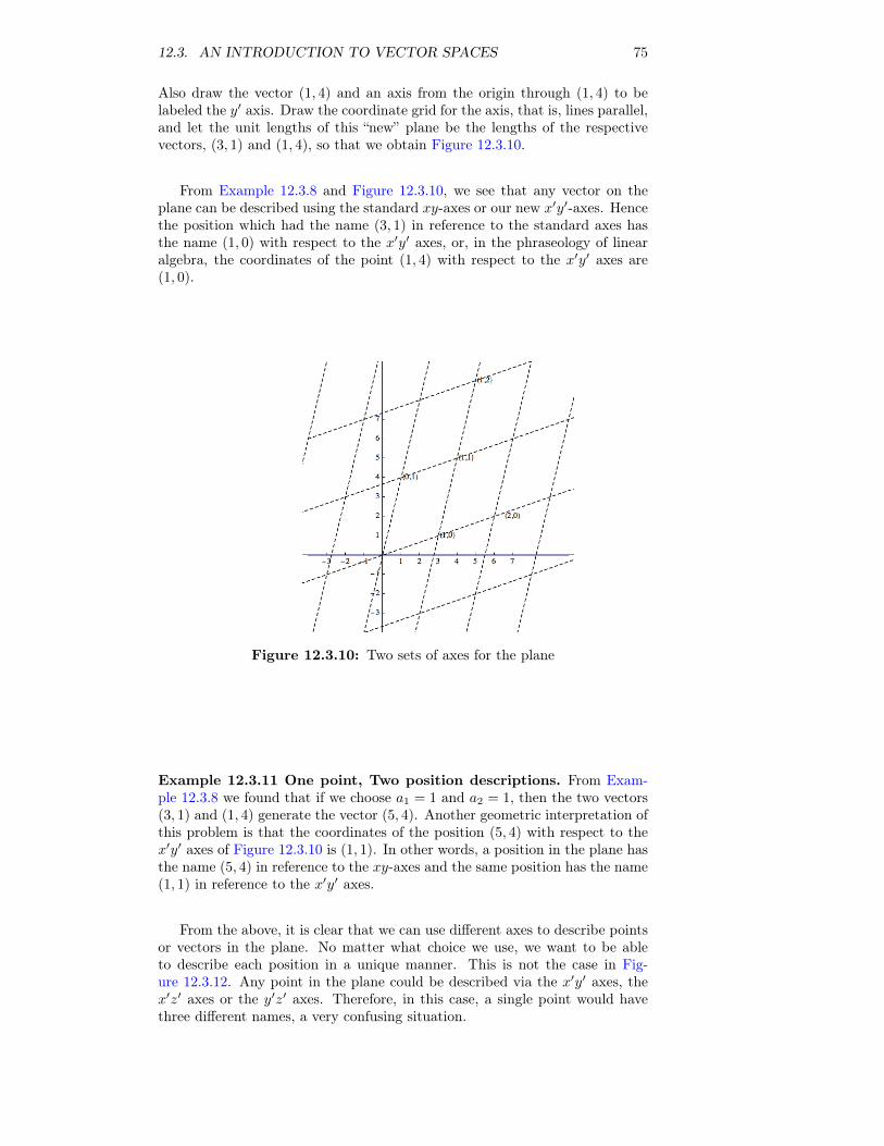
12.3. AN INTRODUCTION TO VECTOR SPACES 75
Also draw the vector (1, 4) and an axis from the origin through (1, 4) to belabeled the y′ axis. Draw the coordinate grid for the axis, that is, lines parallel,and let the unit lengths of this “new” plane be the lengths of the respectivevectors, (3, 1) and (1, 4), so that we obtain Figure 12.3.10.
From Example 12.3.8 and Figure 12.3.10, we see that any vector on theplane can be described using the standard xy-axes or our new x′y′-axes. Hencethe position which had the name (3, 1) in reference to the standard axes hasthe name (1, 0) with respect to the x′y′ axes, or, in the phraseology of linearalgebra, the coordinates of the point (1, 4) with respect to the x′y′ axes are(1, 0).
Figure 12.3.10: Two sets of axes for the plane
Example 12.3.11 One point, Two position descriptions. From Exam-ple 12.3.8 we found that if we choose a1 = 1 and a2 = 1, then the two vectors(3, 1) and (1, 4) generate the vector (5, 4). Another geometric interpretation ofthis problem is that the coordinates of the position (5, 4) with respect to thex′y′ axes of Figure 12.3.10 is (1, 1). In other words, a position in the plane hasthe name (5, 4) in reference to the xy-axes and the same position has the name(1, 1) in reference to the x′y′ axes.
From the above, it is clear that we can use different axes to describe pointsor vectors in the plane. No matter what choice we use, we want to be ableto describe each position in a unique manner. This is not the case in Fig-ure 12.3.12. Any point in the plane could be described via the x′y′ axes, thex′z′ axes or the y′z′ axes. Therefore, in this case, a single point would havethree different names, a very confusing situation.
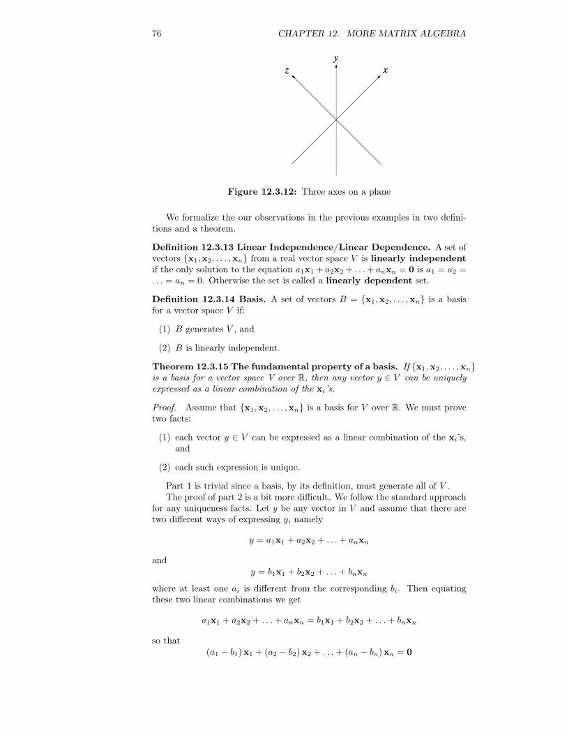
76 CHAPTER 12. MORE MATRIX ALGEBRA
Figure 12.3.12: Three axes on a plane
We formalize the our observations in the previous examples in two defini-tions and a theorem.
Definition 12.3.13 Linear Independence/Linear Dependence. A set ofvectors {x1,x2, . . . ,xn} from a real vector space V is linearly independentif the only solution to the equation a1x1 + a2x2 + . . .+ anxn = 0 is a1 = a2 =. . . = an = 0. Otherwise the set is called a linearly dependent set.
Definition 12.3.14 Basis. A set of vectors B = {x1,x2, . . . ,xn} is a basisfor a vector space V if:
(1) B generates V , and
(2) B is linearly independent.
Theorem 12.3.15 The fundamental property of a basis. If {x1,x2, . . . ,xn}is a basis for a vector space V over R, then any vector y ∈ V can be uniquelyexpressed as a linear combination of the xi’s.
Proof. Assume that {x1,x2, . . . ,xn} is a basis for V over R. We must provetwo facts:
(1) each vector y ∈ V can be expressed as a linear combination of the xi’s,and
(2) each such expression is unique.
Part 1 is trivial since a basis, by its definition, must generate all of V .The proof of part 2 is a bit more difficult. We follow the standard approach
for any uniqueness facts. Let y be any vector in V and assume that there aretwo different ways of expressing y, namely
y = a1x1 + a2x2 + . . .+ anxn
andy = b1x1 + b2x2 + . . .+ bnxn
where at least one ai is different from the corresponding bi. Then equatingthese two linear combinations we get
a1x1 + a2x2 + . . .+ anxn = b1x1 + b2x2 + . . .+ bnxn
so that(a1 − b1)x1 + (a2 − b2)x2 + . . .+ (an − bn)xn = 0
12.3. AN INTRODUCTION TO VECTOR SPACES 77
Now a crucial observation: since the x′is form a linearly independent set, theonly solution to the previous equation is that each of the coefficients must equalzero, so ai− bi = 0 for i = 1, 2, . . . , n. Hence ai = bi, for all i. This contradictsour assumption that at least one ai is different from the corresponding bi, soeach vector y ∈ V can be expressed in one and only one way.
This theorem, together with the previous examples, gives us a clear insightinto the significance of linear independence, namely uniqueness in representingany vector.
Example 12.3.16 Another basis for R2. Prove that {(1, 1), (−1, 1)} is abasis for R2 over R and explain what this means geometrically.
First we show that the vectors (1, 1) and (−1, 1) generate all of R2. Wecan do this by imitating Example 12.3.8 and leave it to the reader (see Exer-cise 12.3.10 of this section). Secondly, we must prove that the set is linearlyindependent.
Let a1 and a2 be scalars such that a1(1, 1) + a2(−1, 1) = (0, 0). We mustprove that the only solution to the equation is that a1 and a2 must both equalzero. The above equation becomes (a1 − a2, a1 + a2) = (0, 0) which gives usthe system
a1 − a2 = 0
a1 + a2 = 0
The augmented matrix of this system reduces in such way that the only solutionis the trivial one of all zeros:(
1 −1 0
1 1 0
)−→
(1 0 0
0 1 0
)⇒ a1 = a2 = 0
Therefore, the set is linearly independent.
To explain the results geometrically, note through Exercise 12, part a, thatthe coordinates of each vector y ∈ R2 can be determined uniquely using thevectors (1,1) and (-1, 1). The concept of dimension is quite obvious for thosevector spaces that have an immediate geometric interpretation. For example,the dimension of R2 is two and that of R3 is three. How can we define theconcept of dimension algebraically so that the resulting definition correlateswith that of R2 and R3? First we need a theorem, which we will state withoutproof.
Theorem 12.3.17 Basis Size is Constant. If V is a vector space with abasis containing n elements, then all bases of V contain n elements.
Definition 12.3.18 Dimension of a Vector Space. Let V be a vector spaceover R with basis {x1,x2, . . . ,xn}. Then the dimension of V is n. We use thenotation dimV = n to indicate that V is n-dimensional.
Exercises for Section 12.3
1. If a = 2, b = −3, A =
(1 0 −1
2 3 4
), B =
(2 −2 3
4 5 8
), and
C =
(1 0 0
3 2 −2
)verify that all properties of the definition of a vector
space are true for M2×3 (R) with these values.2. Let a = 3, b = 4, x === (−1, 3), y = (2, 3),and z = (1, 0). Verify that allproperties of the definition of a vector space are true for R2 for these values.3.
78 CHAPTER 12. MORE MATRIX ALGEBRA
(a) Verify that M2×3 (R) is a vector space over R. What is its dimension?
(b) Is Mm×n (R) a vector space over R? If so, what is its dimension?
4.
(a) Verify that R2 is a vector space over R.
(b) Is Rn a vector space over R for every positive integer n?
5. Let P 3 ={a0 + a1x+ a2x
2 + a3x3 | a0, a1, a2, a3 ∈ R
}; that is, P 3 is the
set of all polynomials in x having real coefficients with degree less than or equalto three. Verify that P 3 is a vector space over R. What is its dimension?6. For each of the following, express the vector yyy as a linear combination ofthe vectors x1 and x2.
(a) y = (5, 6), x1 = (1, 0), and x2 = (0, 1)
(b) y = (2, 1), x1 = (2, 1), and x2 = (1, 1)
(c) y = (3, 4), x1 = (1, 1), and x2 = (−1, 1)
7. Express the vector(
1 2
−3 3
)∈ M2×2(R), as a linear combination of(
1 1
1 1
),(−1 5
2 1
),(
0 1
1 1
)and
(0 0
0 1
)8. Express the vector x3 − 4x2 + 3 ∈ P 3 as a linear combination of thevectors 1, x, x2 , and x3.9.
(a) Show that the set {x1,x2} generates R2 for each of the parts in Exercise6 of this section.
(b) Show that {x1,x2,x3} generates R2 where x1 = (1, 1), x2 = (3, 4), andx3 = (−1, 5).
(c) Create a set of four or more vectors that generates R2.
(d) What is the smallest number of vectors needed to generate R2? Rn?
(e) Show that the set
{A1, A2, A3, A4} = {(
1 0
0 0
),
(0 1
0 0
),
(0 0
1 0
),
(0 0
0 1
)}
generates M2×2(R)
(f) Show that{
1, x, x2, x3}generates P 3.
10. Complete Example 12.3.16 by showing that {(1, 1), (−1, 1)} generatesR2.11.
(a) Prove that {(4, 1), (1, 3)} is a basis for R2 over R.
(b) Prove that {(1, 0), (3, 4)} is a basis for R2 over R.
(c) Prove that {(1, 0,−1), (2, 1, 1), (1,−3,−1)} is a basis for R3 over R.
12.4. THE DIAGONALIZATION PROCESS 79
(d) Prove that the sets in Exercise 9, parts e and f, form bases of the respec-tive vector spaces.
12.
(a) Determine the coordinates of the points or vectors (3, 4), (−1, 1), and(1, 1) with respect to the basis {(1, 1), (−1, 1)} of R3. Interpret yourresults geometrically,
(b) Determine the coordinates of the points or vector (3, 5, 6) with respectto the basis {(1, 0, 0), (0, 1, 0), (0, 0, 1)}. Explain why this basis is calledthe standard basis for R3.
13.
(a) Let y1 = (1, 3, 5, 9), y2 = (5, 7, 6, 3), and c = 2. Find y1 + y2 and cy1.
(b) Let f1(x) = 1 + 3x+ 5x2 + 9x3 , f2(x) = 5 + 7x+ 6x2 + 3x3 and c = 2.Find f1(x) + f2(x) and cf1(x).
(c) Let A =
(1 3
5 9
), B =
(5 7
6 3
), and c = 2. Find A+B and cA.
(d) Are the vector spaces R4 , P 3 and M2×2(R) isomorphic to each other?Discuss with reference to previous parts of this exercise.
12.4 The Diagonalization Process
12.4.1 Eigenvalues and EigenvectorsWe now have the background to understand the main ideas behind the diago-nalization process.
Definition 12.4.1 Eigenvalue, Eigenvector. Let A be an n×n matrix overR. λ is an eigenvalue of A if for some nonzero column vector x ∈ Rn we haveAx = λx. x is called an eigenvector corresponding to the eigenvalue λ.
Example 12.4.2 Examples of eigenvalues and eigenvectors. Find the
eigenvalues and corresponding eigenvectors of the matrix A =
(2 1
2 3
).
We want to find nonzero vectors x =
(x1
x2
)and real numbers λ such that
AX = λX ⇔(
2 1
2 3
)(x1
x2
)= λ
(x1
x2
)⇔(
2 1
2 3
)(x1
x2
)− λ
(x1
x2
)=
(0
0
)⇔(
2 1
2 3
)(x1
x2
)− λ
(1 0
0 1
)(x1
x2
)=
(0
0
)⇔((
2 1
2 3
)− λ
(1 0
0 1
))(x1
x2
)=
(0
0
)⇔(
2− λ 1
2 3− λ
)(x1
x2
)=
(0
0
)(12.4.1)
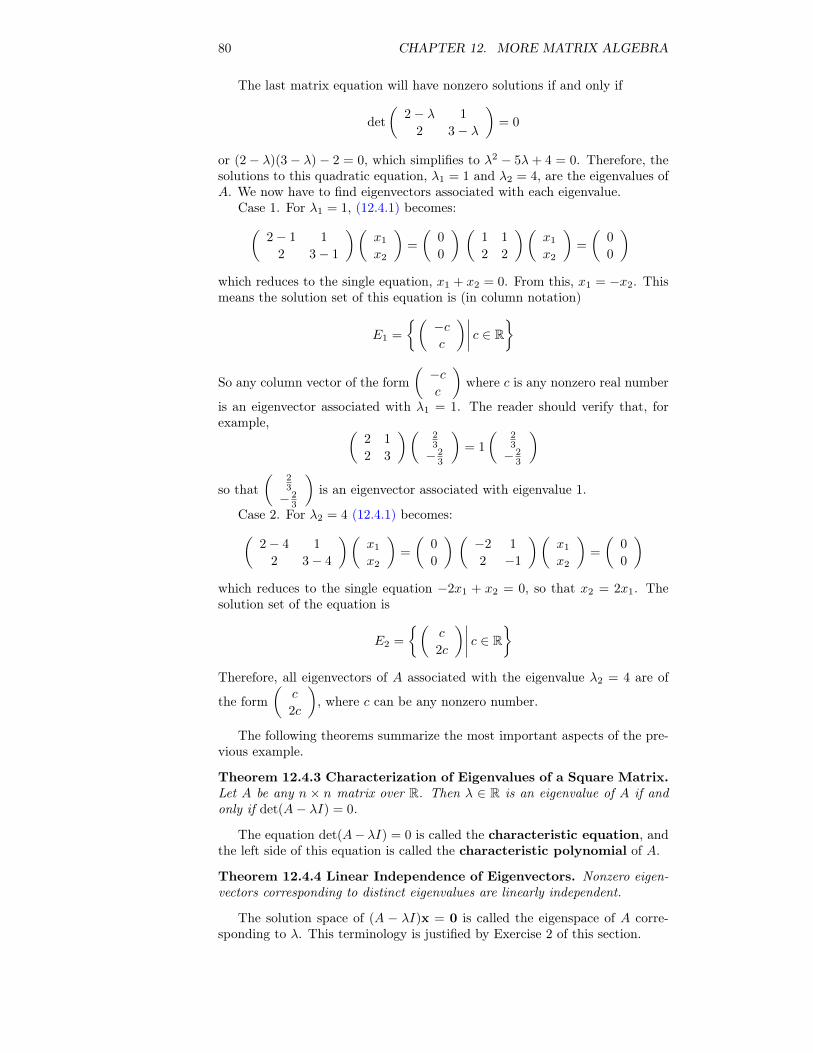
80 CHAPTER 12. MORE MATRIX ALGEBRA
The last matrix equation will have nonzero solutions if and only if
det
(2− λ 1
2 3− λ
)= 0
or (2− λ)(3− λ)− 2 = 0, which simplifies to λ2 − 5λ+ 4 = 0. Therefore, thesolutions to this quadratic equation, λ1 = 1 and λ2 = 4, are the eigenvalues ofA. We now have to find eigenvectors associated with each eigenvalue.
Case 1. For λ1 = 1, (12.4.1) becomes:(2− 1 1
2 3− 1
)(x1
x2
)=
(0
0
) (1 1
2 2
)(x1
x2
)=
(0
0
)which reduces to the single equation, x1 + x2 = 0. From this, x1 = −x2. Thismeans the solution set of this equation is (in column notation)
E1 =
{(−cc
)∣∣∣∣ c ∈ R}
So any column vector of the form(−cc
)where c is any nonzero real number
is an eigenvector associated with λ1 = 1. The reader should verify that, forexample, (
2 1
2 3
)(23
− 23
)= 1
(23
− 23
)so that
(23
− 23
)is an eigenvector associated with eigenvalue 1.
Case 2. For λ2 = 4 (12.4.1) becomes:(2− 4 1
2 3− 4
)(x1
x2
)=
(0
0
) (−2 1
2 −1
)(x1
x2
)=
(0
0
)which reduces to the single equation −2x1 + x2 = 0, so that x2 = 2x1. Thesolution set of the equation is
E2 =
{(c
2c
)∣∣∣∣ c ∈ R}Therefore, all eigenvectors of A associated with the eigenvalue λ2 = 4 are of
the form(
c
2c
), where c can be any nonzero number.
The following theorems summarize the most important aspects of the pre-vious example.
Theorem 12.4.3 Characterization of Eigenvalues of a Square Matrix.Let A be any n × n matrix over R. Then λ ∈ R is an eigenvalue of A if andonly if det(A− λI) = 0.
The equation det(A− λI) = 0 is called the characteristic equation, andthe left side of this equation is called the characteristic polynomial of A.
Theorem 12.4.4 Linear Independence of Eigenvectors. Nonzero eigen-vectors corresponding to distinct eigenvalues are linearly independent.
The solution space of (A − λI)x = 0 is called the eigenspace of A corre-sponding to λ. This terminology is justified by Exercise 2 of this section.
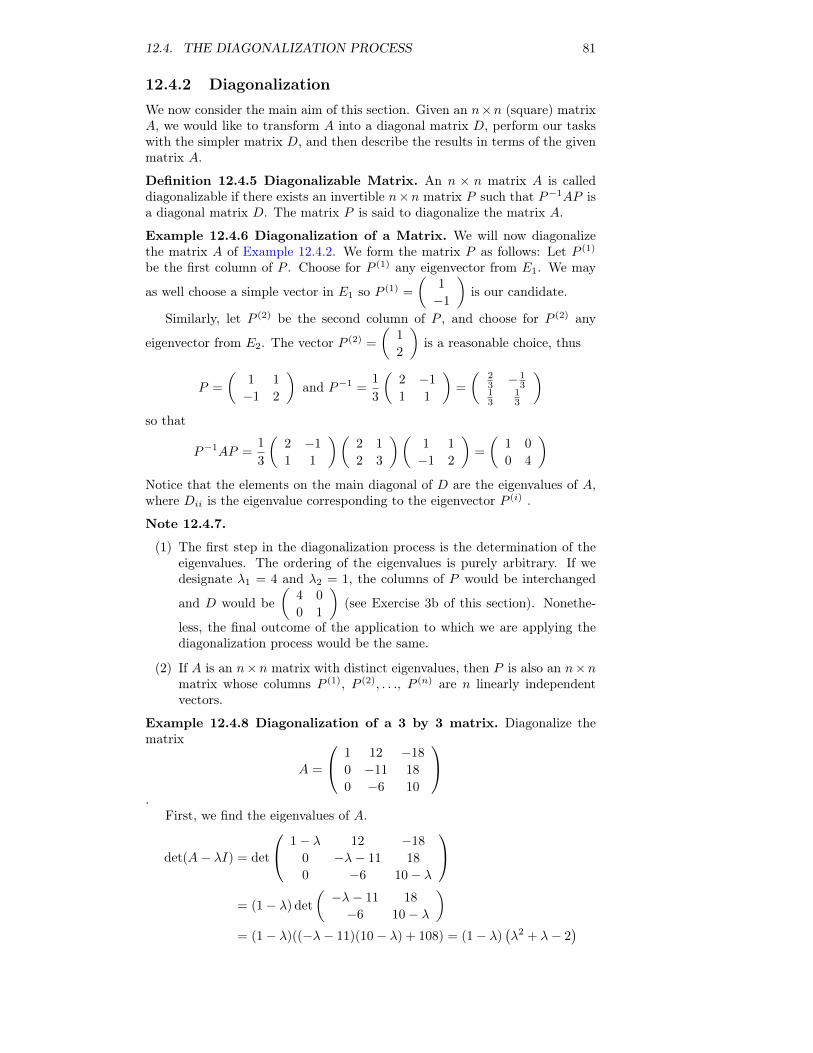
12.4. THE DIAGONALIZATION PROCESS 81
12.4.2 DiagonalizationWe now consider the main aim of this section. Given an n×n (square) matrixA, we would like to transform A into a diagonal matrix D, perform our taskswith the simpler matrix D, and then describe the results in terms of the givenmatrix A.
Definition 12.4.5 Diagonalizable Matrix. An n × n matrix A is calleddiagonalizable if there exists an invertible n×n matrix P such that P−1AP isa diagonal matrix D. The matrix P is said to diagonalize the matrix A.
Example 12.4.6 Diagonalization of a Matrix. We will now diagonalizethe matrix A of Example 12.4.2. We form the matrix P as follows: Let P (1)
be the first column of P . Choose for P (1) any eigenvector from E1. We may
as well choose a simple vector in E1 so P (1) =
(1
−1
)is our candidate.
Similarly, let P (2) be the second column of P , and choose for P (2) any
eigenvector from E2. The vector P (2) =
(1
2
)is a reasonable choice, thus
P =
(1 1
−1 2
)and P−1 =
1
3
(2 −1
1 1
)=
(23 − 1
313
13
)so that
P−1AP =1
3
(2 −1
1 1
)(2 1
2 3
)(1 1
−1 2
)=
(1 0
0 4
)Notice that the elements on the main diagonal of D are the eigenvalues of A,where Dii is the eigenvalue corresponding to the eigenvector P (i) .
Note 12.4.7.
(1) The first step in the diagonalization process is the determination of theeigenvalues. The ordering of the eigenvalues is purely arbitrary. If wedesignate λ1 = 4 and λ2 = 1, the columns of P would be interchanged
and D would be(
4 0
0 1
)(see Exercise 3b of this section). Nonethe-
less, the final outcome of the application to which we are applying thediagonalization process would be the same.
(2) If A is an n×n matrix with distinct eigenvalues, then P is also an n×nmatrix whose columns P (1), P (2), . . ., P (n) are n linearly independentvectors.
Example 12.4.8 Diagonalization of a 3 by 3 matrix. Diagonalize thematrix
A =
1 12 −18
0 −11 18
0 −6 10
.
First, we find the eigenvalues of A.
det(A− λI) = det
1− λ 12 −18
0 −λ− 11 18
0 −6 10− λ
= (1− λ) det
(−λ− 11 18
−6 10− λ
)= (1− λ)((−λ− 11)(10− λ) + 108) = (1− λ)
(λ2 + λ− 2
)
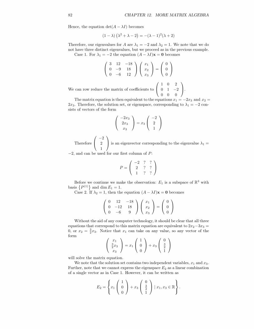
82 CHAPTER 12. MORE MATRIX ALGEBRA
Hence, the equation det(A− λI) becomes
(1− λ)(λ2 + λ− 2
)= −(λ− 1)2(λ+ 2)
Therefore, our eigenvalues for A are λ1 = −2 and λ2 = 1. We note that we donot have three distinct eigenvalues, but we proceed as in the previous example.
Case 1. For λ1 = −2 the equation (A− λI)x = 0 becomes 3 12 −18
0 −9 18
0 −6 12
x1
x2
x3
=
0
0
0
We can row reduce the matrix of coefficients to
1 0 2
0 1 −2
0 0 0
.
The matrix equation is then equivalent to the equations x1 = −2x3 and x2 =2x3. Therefore, the solution set, or eigenspace, corresponding to λ1 = −2 con-sists of vectors of the form −2x3
2x3
x3
= x3
−2
2
1
Therefore
−2
2
1
is an eigenvector corresponding to the eigenvalue λ1 =
−2, and can be used for our first column of P :
P =
−2 ? ?
2 ? ?
1 ? ?
Before we continue we make the observation: E1 is a subspace of R3 with
basis{P (1)
}and dimE1 = 1.
Case 2. If λ2 = 1, then the equation (A− λI)x = 0 becomes 0 12 −18
0 −12 18
0 −6 9
x1
x2
x3
=
0
0
0
Without the aid of any computer technology, it should be clear that all three
equations that correspond to this matrix equation are equivalent to 2x2−3x3 =0, or x2 = 3
2x3. Notice that x1 can take on any value, so any vector of theform x1
32x3
x3
= x1
1
0
0
+ x3
032
1
will solve the matrix equation.
We note that the solution set contains two independent variables, x1 and x3.Further, note that we cannot express the eigenspace E2 as a linear combinationof a single vector as in Case 1. However, it can be written as
E2 =
x1
1
0
0
+ x3
032
1
| x1, x3 ∈ R
.
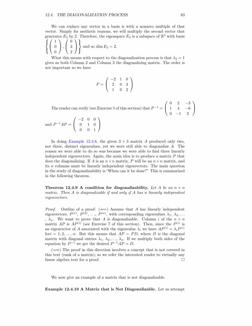
12.4. THE DIAGONALIZATION PROCESS 83
We can replace any vector in a basis is with a nonzero multiple of thatvector. Simply for aesthetic reasons, we will multiply the second vector thatgenerates E2 by 2. Therefore, the eigenspace E2 is a subspace of R3 with basis 1
0
0
,
0
3
2
and so dimE2 = 2.
What this means with respect to the diagonalization process is that λ2 = 1gives us both Column 2 and Column 3 the diagonalizing matrix. The order isnot important so we have
P =
−2 1 0
2 0 3
1 0 2
The reader can verify (see Exercise 5 of this section) that P−1 =
0 2 −3
1 4 −6
0 −1 2
and P−1AP =
−2 0 0
0 1 0
0 0 1
In doing Example 12.4.8, the given 3 × 3 matrix A produced only two,
not three, distinct eigenvalues, yet we were still able to diagonalize A. Thereason we were able to do so was because we were able to find three linearlyindependent eigenvectors. Again, the main idea is to produce a matrix P thatdoes the diagonalizing. If A is an n×n matrix, P will be an n×n matrix, andits n columns must be linearly independent eigenvectors. The main questionin the study of diagonalizability is “When can it be done?” This is summarizedin the following theorem.
Theorem 12.4.9 A condition for diagonalizability. Let A be an n × nmatrix. Then A is diagonalizable if and only if A has n linearly independenteigenvectors.
Proof. Outline of a proof: (⇐=) Assume that A has linearly independenteigenvectors, P (1), P (2), . . ., P (n), with corresponding eigenvalues λ1, λ2, . . ., λn. We want to prove that A is diagonalizable. Column i of the n × nmatrix AP is AP (i) (see Exercise 7 of this section). Then, since the P (i) isan eigenvector of A associated with the eigenvalue λi we have AP (i) = λiP
(i)
fori = 1, 2, . . . , n. But this means that AP = PD, where D is the diagonalmatrix with diagonal entries λ1, λ2, . . ., λn. If we multiply both sides of theequation by P−1 we get the desired P−1AP = D.
(=⇒) The proof in this direction involves a concept that is not covered inthis text (rank of a matrix); so we refer the interested reader to virtually anylinear algebra text for a proof.
We now give an example of a matrix that is not diagonalizable.
Example 12.4.10 A Matrix that is Not Diagonalizable. Let us attempt
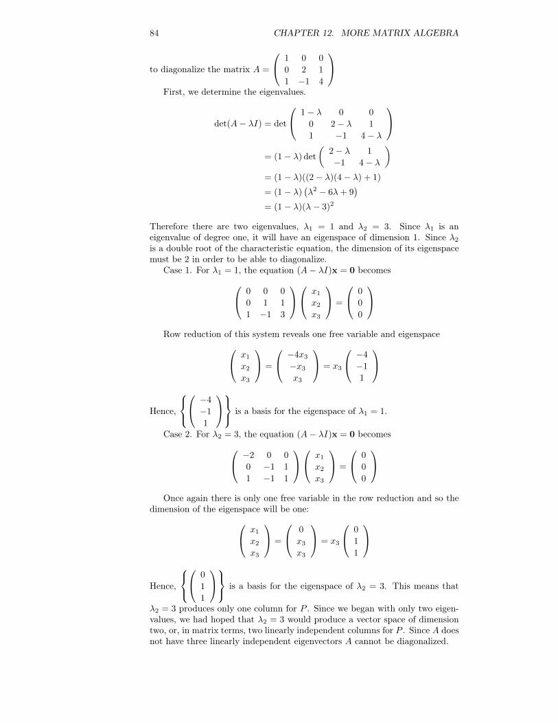
84 CHAPTER 12. MORE MATRIX ALGEBRA
to diagonalize the matrix A =
1 0 0
0 2 1
1 −1 4
First, we determine the eigenvalues.
det(A− λI) = det
1− λ 0 0
0 2− λ 1
1 −1 4− λ
= (1− λ) det
(2− λ 1
−1 4− λ
)= (1− λ)((2− λ)(4− λ) + 1)
= (1− λ)(λ2 − 6λ+ 9
)= (1− λ)(λ− 3)2
Therefore there are two eigenvalues, λ1 = 1 and λ2 = 3. Since λ1 is aneigenvalue of degree one, it will have an eigenspace of dimension 1. Since λ2
is a double root of the characteristic equation, the dimension of its eigenspacemust be 2 in order to be able to diagonalize.
Case 1. For λ1 = 1, the equation (A− λI)x = 0 becomes 0 0 0
0 1 1
1 −1 3
x1
x2
x3
=
0
0
0
Row reduction of this system reveals one free variable and eigenspace x1
x2
x3
=
−4x3
−x3
x3
= x3
−4
−1
1
Hence,
−4
−1
1
is a basis for the eigenspace of λ1 = 1.
Case 2. For λ2 = 3, the equation (A− λI)x = 0 becomes −2 0 0
0 −1 1
1 −1 1
x1
x2
x3
=
0
0
0
Once again there is only one free variable in the row reduction and so the
dimension of the eigenspace will be one: x1
x2
x3
=
0
x3
x3
= x3
0
1
1
Hence,
0
1
1
is a basis for the eigenspace of λ2 = 3. This means that
λ2 = 3 produces only one column for P . Since we began with only two eigen-values, we had hoped that λ2 = 3 would produce a vector space of dimensiontwo, or, in matrix terms, two linearly independent columns for P . Since A doesnot have three linearly independent eigenvectors A cannot be diagonalized.
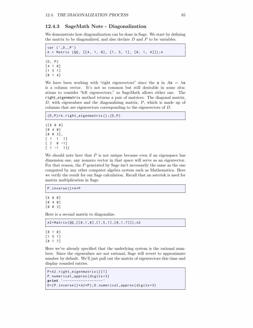
12.4. THE DIAGONALIZATION PROCESS 85
12.4.3 SageMath Note - Diagonalization
We demonstrate how diagonalization can be done in Sage. We start by definingthe matrix to be diagonalized, and also declare D and P to be variables.
var ('␣D,␣P')A = Matrix (QQ, [[4, 1, 0], [1, 5, 1], [0, 1, 4]]);A
(D, P)[4 1 0][1 5 1][0 1 4]
We have been working with “right eigenvectors” since the x in Ax = λxis a column vector. It’s not so common but still desirable in some situ-ations to consider “left eigenvectors,” so SageMath allows either one. Theright_eigenmatrix method returns a pair of matrices. The diagonal matrix,D, with eigenvalues and the diagonalizing matrix, P , which is made up ofcolumns that are eigenvectors corresponding to the eigenvectors of D.
(D,P)=A.right_eigenmatrix ();(D,P)
([6 0 0][0 4 0][0 0 3],[ 1 1 1][ 2 0 -1][ 1 -1 1])
We should note here that P is not unique because even if an eigenspace hasdimension one, any nonzero vector in that space will serve as an eigenvector.For that reason, the P generated by Sage isn’t necessarily the same as the onecomputed by any other computer algebra system such as Mathematica. Herewe verify the result for our Sage calculation. Recall that an asterisk is used formatrix multiplication in Sage.
P.inverse ()*A*P
[6 0 0][0 4 0][0 0 3]
Here is a second matrix to diagonalize.
A2=Matrix(QQ ,[[8,1,0],[1,5,1],[0,1,7]]);A2
[8 1 0][1 5 1][0 1 7]
Here we’ve already specified that the underlying system is the rational num-bers. Since the eigenvalues are not rational, Sage will revert to approximatenumber by default. We’ll just pull out the matrix of eigenvectors this time anddisplay rounded entries.
P=A2.right_eigenmatrix ()[1]P.numerical_approx(digits =3)print '------------------'D=(P.inverse ()*A2*P);D.numerical_approx(digits =3)
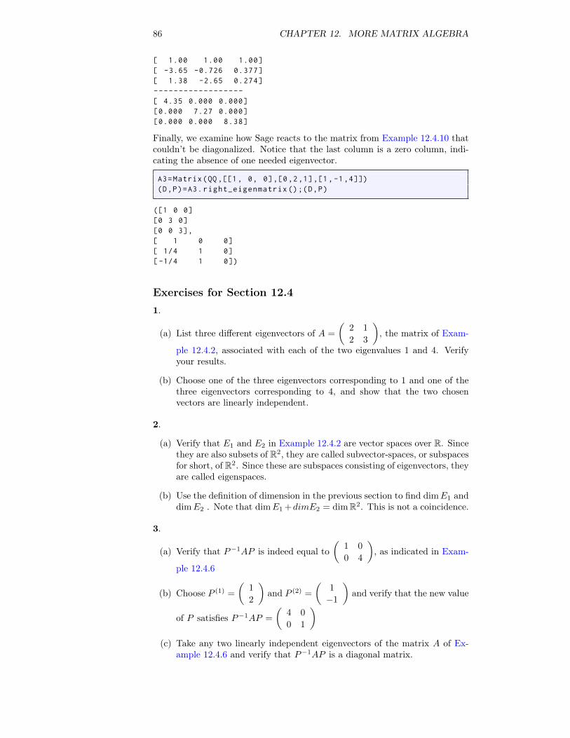
86 CHAPTER 12. MORE MATRIX ALGEBRA
[ 1.00 1.00 1.00][ -3.65 -0.726 0.377][ 1.38 -2.65 0.274]------------------[ 4.35 0.000 0.000][0.000 7.27 0.000][0.000 0.000 8.38]
Finally, we examine how Sage reacts to the matrix from Example 12.4.10 thatcouldn’t be diagonalized. Notice that the last column is a zero column, indi-cating the absence of one needed eigenvector.
A3=Matrix(QQ ,[[1, 0, 0],[0,2,1],[1,-1,4]])(D,P)=A3.right_eigenmatrix ();(D,P)
([1 0 0][0 3 0][0 0 3],[ 1 0 0][ 1/4 1 0][-1/4 1 0])
Exercises for Section 12.4
1.
(a) List three different eigenvectors of A =
(2 1
2 3
), the matrix of Exam-
ple 12.4.2, associated with each of the two eigenvalues 1 and 4. Verifyyour results.
(b) Choose one of the three eigenvectors corresponding to 1 and one of thethree eigenvectors corresponding to 4, and show that the two chosenvectors are linearly independent.
2.
(a) Verify that E1 and E2 in Example 12.4.2 are vector spaces over R. Sincethey are also subsets of R2, they are called subvector-spaces, or subspacesfor short, of R2. Since these are subspaces consisting of eigenvectors, theyare called eigenspaces.
(b) Use the definition of dimension in the previous section to find dimE1 anddimE2 . Note that dimE1 +dimE2 = dimR2. This is not a coincidence.
3.
(a) Verify that P−1AP is indeed equal to(
1 0
0 4
), as indicated in Exam-
ple 12.4.6
(b) Choose P (1) =
(1
2
)and P (2) =
(1
−1
)and verify that the new value
of P satisfies P−1AP =
(4 0
0 1
)(c) Take any two linearly independent eigenvectors of the matrix A of Ex-
ample 12.4.6 and verify that P−1AP is a diagonal matrix.
12.5. SOME APPLICATIONS 87
4.
(a) Let A be the matrix in Example 12.4.8 and P =
0 1 0
1 0 1
1 0 2
. Without
doing any actual matrix multiplications, determine the value of P−1AP
(b) If you choose the columns of P in the reverse order, what is P−1AP?
5. Diagonalize the following, if possible:
(a)(
1 2
3 2
)
(b)(−2 1
−7 6
)(c)
(3 0
0 4
)
(d)
1 −1 4
3 2 −1
2 1 −1
(e)
6 0 0
0 7 −4
9 1 3
(f)
1 −1 0
−1 2 −1
0 −1 1
6. Diagonalize the following, if possible:
(a)(
0 1
1 1
)
(b)(
2 1
4 2
)(c)
(2 −1
1 0
)
(d)
1 3 6
−3 −5 −6
3 3 6
(e)
1 1 0
1 0 1
0 1 1
(f)
2 −1 0
−1 2 −1
0 −1 2
7. Let A and P be as in Example 12.4.8. Show that the columns of thematrix AP can be found by computing AP (1), AP (2), . . . , AP (n).8. Prove that if P is an n × n matrix and D is a diagonal matrix withdiagonal entries d1, d2, . . . , dn, then PD is the matrix obtained from P , bymultiplying column i of P by di, i = 1, 2, . . . , n.
12.5 Some ApplicationsA large and varied number of applications involve computations of powersof matrices. These applications can be found in science, the social sciences,economics, engineering, and, many other areas where mathematics is used. Wewill consider a few diverse examples the mathematics behind these applicationshere.
12.5.1 DiagonalizationWe begin by developing a helpful technique for computing Am, m > 1. If Acan be diagonalized, then there is a matrix P such that P−1AP = D, whereD is a diagonal matrix and
Am = PDmP−1 for all m ≥ 1 (12.5.1)
The proof of this identity was an exercise in Section 5.4. The conditionthat D be a diagonal matrix is not necessary but when it is, the calculation
88 CHAPTER 12. MORE MATRIX ALGEBRA
on the right side is particularly easy to perform. Although the formal proof isdone by induction, the reason why it is true is easily seen by writing out anexample such as m = 3:
A3 =(PDP−1
)3=(PDP−1
) (PDP−1
) (PDP−1
)= PD
(P−1P
)D(P−1P
)DP−1 by associativity of matrix multiplication
= PDIDIDP−1
= PDDDP−1
= PD3P−1
Example 12.5.1 Application to Recursion: Matrix Computation ofthe Fibonnaci Sequence. Consider the computation of terms of the Fibon-naci Sequence. Recall that F0 = 1, F1 = 1 and Fk = Fk−1 + Fk−2 for k ≥ 2.
In order to formulate the calculation in matrix form, we introduced the“dummy equation” Fk−1 = Fk−1 so that now we have two equations
Fk = Fk−1 + Fk−2
Fk−1 = Fk−1
If A =
(1 1
1 0
), these two equations can be expressed in matrix form as
(FkFk−1
)=
(1 1
1 0
)(Fk−1
Fk−2
)if k ≥ 2
= A
(Fk−1
Fk−2
)= A2
(Fk−2
Fk−3
)if k ≥ 3
etc.
We can use induction to prove that if k ≥ 2,(FkFk−1
)= Ak−1
(1
1
)Next, by diagonalizing A and using the fact that Am = PDmP−1. we can
show that
Fk =1√5
(1 +√
5
2
)k−
(1−√
5
2
)kSome comments on this example:
(1) An equation of the form Fk = aFk−1 + bFk−2 , where a and b are givenconstants, is referred to as a linear homogeneous second-order differenceequation. The conditions F0 = c0 and F1 = c1 , where c1 and c2 are con-stants, are called initial conditions. Those of you who are familiar withdifferential equations may recognize that this language parallels what isused in differential equations. Difference (aka recurrence) equations moveforward discretely; that is, in a finite number of positive steps. On theother hand, a differential equation moves continuously; that is, takes aninfinite number of infinitesimal steps.
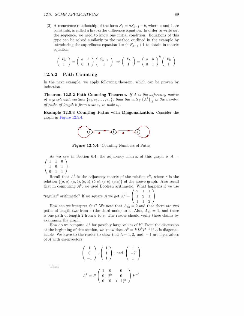
12.5. SOME APPLICATIONS 89
(2) A recurrence relationship of the form Sk = aSk−1 + b, where a and b areconstants, is called a first-order difference equation. In order to write outthe sequence, we need to know one initial condition. Equations of thistype can be solved similarly to the method outlined in the example byintroducing the superfluous equation 1 = 0 ·Fk−1 + 1 to obtain in matrixequation:(
Fk1
)=
(a b
0 1
)(Sk−1
1
)⇒(Fk1
)=
(a b
0 1
)k (F0
1
)
12.5.2 Path CountingIn the next example, we apply following theorem, which can be proven byinduction.
Theorem 12.5.2 Path Counting Theorem. If A is the adjacency matrixof a graph with vertices {v1, v2, . . . , vn}, then the entry
(Ak)ij
is the numberof paths of length k from node vi to node vj.
Example 12.5.3 Counting Paths with Diagonalization. Consider thegraph in Figure 12.5.4.
Figure 12.5.4: Counting Numbers of Paths
As we saw in Section 6.4, the adjacency matrix of this graph is A = 1 1 0
1 0 1
0 1 1
.
Recall that Ak is the adjacency matrix of the relation rk, where r is therelation {(a, a), (a, b), (b, a), (b, c), (c, b), (c, c)} of the above graph. Also recallthat in computing Ak, we used Boolean arithmetic. What happens if we use
“regular” arithmetic? If we square A we get A2 =
2 1 1
1 2 1
1 1 2
How can we interpret this? We note that A33 = 2 and that there are two
paths of length two from c (the third node) to c. Also, A13 = 1, and thereis one path of length 2 from a to c. The reader should verify these claims byexamining the graph.
How do we compute Ak for possibly large values of k? From the discussionat the beginning of this section, we know that Ak = PDkP−1 if A is diagonal-izable. We leave to the reader to show that λ = 1, 2, and − 1 are eigenvaluesof A with eigenvectors 1
0
−1
,
1
1
1
, and
1
−2
1
Then
Ak = P
1 0 0
0 2k 0
0 0 (−1)k
P−1
90 CHAPTER 12. MORE MATRIX ALGEBRA
where P =
1 1 1
0 1 −2
−1 1 1
and P−1 =
12 0 − 1
213
13
13
16 − 1
316
See Exercise 12.5.5 of this section for the completion of this example.
12.5.3 Matrix CalculusExample 12.5.5 Matrix Calculus - Exponentials. Those who have stud-ied calculus recall that the Maclaurin series is a useful way of expressing manycommon functions. For example, ex =
∑∞k=0
xk
k! . Indeed, calculators and com-puters use these series for calculations. Given a polynomial f(x), we definedthe matrix-polynomial f(A) for square matrices in Chapter 5. Hence, we arein a position to describe eA for an n × n matrix A as a limit of polynomials,the partial sums of the series. Formally, we write
eA = I +A+A2
2!+A3
3!+ · · · =
∞∑k=0
Ak
k!
Again we encounter the need to compute high powers of a matrix. Let Abe an n×n diagonalizable matrix. Then there exists an invertible n×n matrixP such that P−1AP = D, a diagonal matrix, so that
eA = ePDP−1
=
∞∑k=0
(PDP−1
)kk!
= P
( ∞∑k=0
Dk
k!
)P−1
The infinite sum in the middle of this final expression can be easily evaluatedif D is diagonal. All entries of powers off the diagonal are zero and the i th
entry of the diagonal is( ∞∑k=0
Dk
k!
)ii =
∞∑k=0
Diik
k!= eDii
For example, if A =
(2 1
2 3
), the first matrix we diagonalized in Section
12.3, we found that P =
(1 1
−1 2
)and D =
(1 0
0 4
).
Therefore,
eA =
(1 1
−1 2
)(e 0
0 e4
)(23 − 1
313
13
)=
(2e3 + e4
3 − e3 + e4
3
− 2e3 + 2e4
3e3 + 2e4
3
)
≈(
20.0116 17.2933
34.5866 37.3049
)Remark 12.5.6. Many of the ideas of calculus can be developed using matri-
ces. For example, if A(t) =
(t3 3t2 + 8t
et 2
)then dA(t)
dt =
(3t2 6t+ 8
et 0
)Many of the basic formulas in calculus are true in matrix calculus. For
12.5. SOME APPLICATIONS 91
example,
d(A(t) +B(t))
dt=dA(t)
dt+dB(t)
dt
and if A is a constant matrix,
deAt
dt= AeAt
Matrix calculus can be used to solve systems of differential equations in asimilar manner to the procedure used in ordinary differential equations.
12.5.4 SageMath Note - Matrix Exponential
Sage’s matrix exponential method is exp.
A=Matrix(QQ ,[[2 ,1] ,[2 ,3]])A.exp()
[1/3*e^4 + 2/3*e 1/3*e^4 - 1/3*e][2/3*e^4 - 2/3*e 2/3*e^4 + 1/3*e]
Exercises for Section 12.5
1.
(a) Write out all the details of Example 12.5.1 to show that the formula forFk given in the text is correct.
(b) Use induction to prove the assertion made in the example that(
FkFk−1
)=
Ak−1
(1
1
)
2.
(a) Do Example 8.0.2 using the method outlined in Example 12.5.1. Notethat the terminology characteristic equation, characteristic polynomial,and so on, introduced in Chapter 8, comes from the language of matrixalgebra,
(b) What is the significance of Algorithm 8.0.1, part c, with respect to thissection?
3. Solve S(k) = 5S(k − 1) + 4, with S(0) = 0, using the method of thissection.
4. How many paths are there of length 6 from vertex 1 to vertex 3 inFigure B.0.2? How many paths from vertex 2 to vertex 2 of length 6 are there?
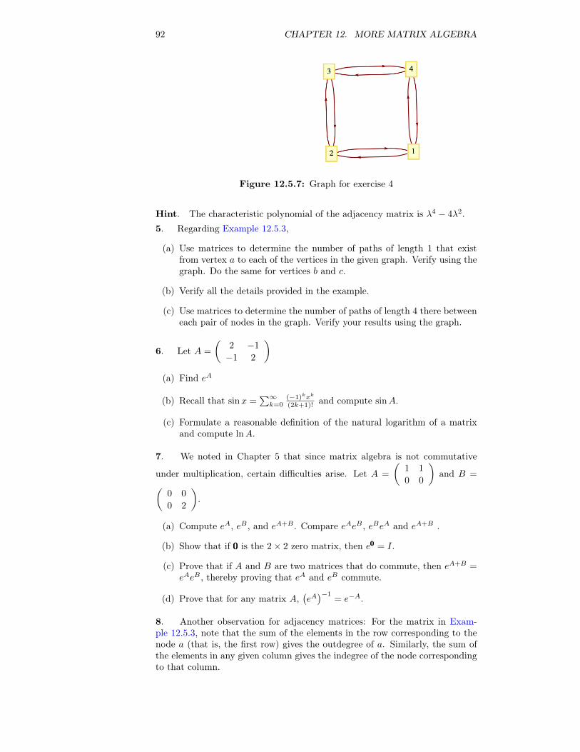
92 CHAPTER 12. MORE MATRIX ALGEBRA
Figure 12.5.7: Graph for exercise 4
Hint. The characteristic polynomial of the adjacency matrix is λ4 − 4λ2.5. Regarding Example 12.5.3,
(a) Use matrices to determine the number of paths of length 1 that existfrom vertex a to each of the vertices in the given graph. Verify using thegraph. Do the same for vertices b and c.
(b) Verify all the details provided in the example.
(c) Use matrices to determine the number of paths of length 4 there betweeneach pair of nodes in the graph. Verify your results using the graph.
6. Let A =
(2 −1
−1 2
)(a) Find eA
(b) Recall that sinx =∑∞k=0
(−1)kxk
(2k+1)! and compute sinA.
(c) Formulate a reasonable definition of the natural logarithm of a matrixand compute lnA.
7. We noted in Chapter 5 that since matrix algebra is not commutative
under multiplication, certain difficulties arise. Let A =
(1 1
0 0
)and B =(
0 0
0 2
).
(a) Compute eA, eB , and eA+B . Compare eAeB , eBeA and eA+B .
(b) Show that if 000 is the 2× 2 zero matrix, then e000 = I.
(c) Prove that if A and B are two matrices that do commute, then eA+B =eAeB , thereby proving that eA and eB commute.
(d) Prove that for any matrix A,(eA)−1
= e−A.
8. Another observation for adjacency matrices: For the matrix in Exam-ple 12.5.3, note that the sum of the elements in the row corresponding to thenode a (that is, the first row) gives the outdegree of a. Similarly, the sum ofthe elements in any given column gives the indegree of the node correspondingto that column.
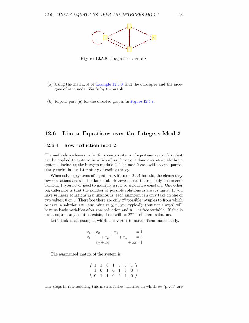
12.6. LINEAR EQUATIONS OVER THE INTEGERS MOD 2 93
Figure 12.5.8: Graph for exercise 8
(a) Using the matrix A of Example 12.5.3, find the outdegree and the inde-gree of each node. Verify by the graph.
(b) Repeat part (a) for the directed graphs in Figure 12.5.8.
12.6 Linear Equations over the Integers Mod 2
12.6.1 Row reduction mod 2
The methods we have studied for solving systems of equations up to this pointcan be applied to systems in which all arithmetic is done over other algebraicsystems, including the integers modulo 2. The mod 2 case will become partic-ularly useful in our later study of coding theory.
When solving systems of equations with mod 2 arithmetic, the elementaryrow operations are still fundamental. However, since there is only one nozeroelement, 1, you never need to multiply a row by a nonzero constant. One otherbig difference is that the number of possible solutions is always finite. If youhave m linear equations in n unknowns, each unknown can only take on one oftwo values, 0 or 1. Therefore there are only 2n possible n-tuples to from whichto draw a solution set. Assuming m ≤ n, you typically (but not always) willhave m basic variables after row-reduction and n −m free variable. If this isthe case, and any solution exists, there will be 2n−m different solutions.
Let’s look at an example, which is coverted to matrix form immediately.
x1 + x2 + x4 = 1
x1 + x3 + x5 = 0
x2 + x3 + x6= 1
The augmented matrix of the system is
1 1 0 1 0 0 1
1 0 1 0 1 0 0
0 1 1 0 0 1 0
The steps in row-reducing this matrix follow. Entries on which we “pivot” are
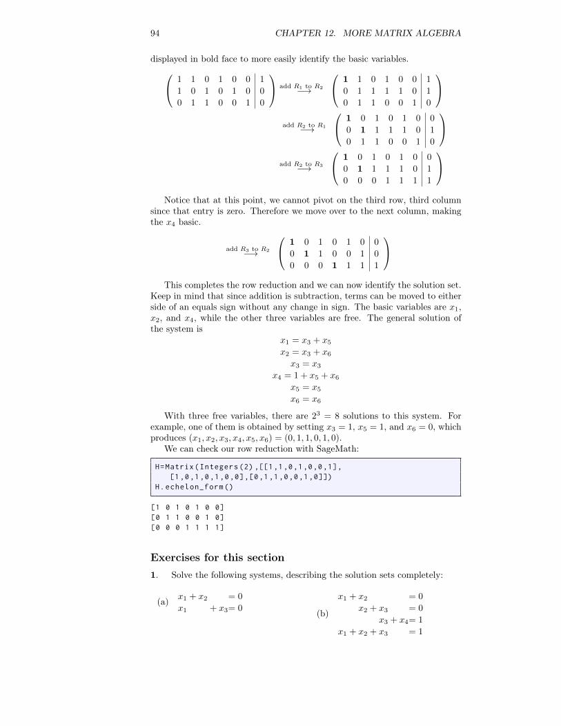
94 CHAPTER 12. MORE MATRIX ALGEBRA
displayed in bold face to more easily identify the basic variables. 1 1 0 1 0 0 1
1 0 1 0 1 0 0
0 1 1 0 0 1 0
add R1 to R2−→
1 1 0 1 0 0 1
0 1 1 1 1 0 1
0 1 1 0 0 1 0
add R2 to R1−→
1 0 1 0 1 0 0
0 1 1 1 1 0 1
0 1 1 0 0 1 0
add R2 to R3−→
1 0 1 0 1 0 0
0 1 1 1 1 0 1
0 0 0 1 1 1 1
Notice that at this point, we cannot pivot on the third row, third column
since that entry is zero. Therefore we move over to the next column, makingthe x4 basic.
add R3 to R2−→
1 0 1 0 1 0 0
0 1 1 0 0 1 0
0 0 0 1 1 1 1
This completes the row reduction and we can now identify the solution set.
Keep in mind that since addition is subtraction, terms can be moved to eitherside of an equals sign without any change in sign. The basic variables are x1,x2, and x4, while the other three variables are free. The general solution ofthe system is
x1 = x3 + x5
x2 = x3 + x6
x3 = x3
x4 = 1 + x5 + x6
x5 = x5
x6 = x6
With three free variables, there are 23 = 8 solutions to this system. Forexample, one of them is obtained by setting x3 = 1, x5 = 1, and x6 = 0, whichproduces (x1, x2, x3, x4, x5, x6) = (0, 1, 1, 0, 1, 0).
We can check our row reduction with SageMath:
H=Matrix(Integers (2) ,[[1,1,0,1,0,0,1],[1,0,1,0,1,0,0],[0,1,1,0,0,1,0]])
H.echelon_form ()
[1 0 1 0 1 0 0][0 1 1 0 0 1 0][0 0 0 1 1 1 1]
Exercises for this section1. Solve the following systems, describing the solution sets completely:
(a) x1 + x2 = 0
x1 + x3= 0 (b)
x1 + x2 = 0
x2 + x3 = 0
x3 + x4= 1
x1 + x2 + x3 = 1
12.6. LINEAR EQUATIONS OVER THE INTEGERS MOD 2 95
2. This exercise provides an example in which the number of basic variablesis less than the number of equations. The only difference between the twosystems below is the right hand sides. You can start with an augmentedmatrix having to right side columns and do row reduction for both systems atthe same time.
(a)x1 + x2 + x4= 1
x1 + x3 + x4= 0
x2 + x3 = 1
(b)x1 + x2 + x4= 1
x1 + x3 + x4= 0
x2 + x3 = 0
3. This exercise motivates the concept of a coset in Chapter 15.
(a) Solve the following system and prove that the solution set is a linearcombination of vectors in Z5
2 and also a subgroup of the group Z52 under
coordinatewise mod 2 addition.
x1 + x2 + x5= 0
x1 + x3 + x5= 0
x1 + x3 + x4 = 0
x2 + x3 + x4 = 0
(b) Describe the solution set to the following system as it relates to thesolution set to the system in the previous part of this exercise.
x1 + x2 + x5= 1
x1 + x3 + x5= 0
x1 + x3 + x4 = 1
x2 + x3 + x4 = 0

96 CHAPTER 12. MORE MATRIX ALGEBRA
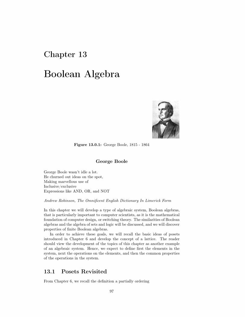
Chapter 13
Boolean Algebra
Figure 13.0.1: George Boole, 1815 - 1864
George Boole
George Boole wasn’t idle a lot.He churned out ideas on the spot,Making marvellous use ofInclusive/exclusiveExpressions like AND, OR, and NOT
Andrew Robinson, The Omnificent English Dictionary In Limerick Form
In this chapter we will develop a type of algebraic system, Boolean algebras,that is particularly important to computer scientists, as it is the mathematicalfoundation of computer design, or switching theory. The similarities of Booleanalgebras and the algebra of sets and logic will be discussed, and we will discoverproperties of finite Boolean algebras.
In order to achieve these goals, we will recall the basic ideas of posetsintroduced in Chapter 6 and develop the concept of a lattice. The readershould view the development of the topics of this chapter as another exampleof an algebraic system. Hence, we expect to define first the elements in thesystem, next the operations on the elements, and then the common propertiesof the operations in the system.
13.1 Posets Revisited
From Chapter 6, we recall the definition a partially ordering
97
98 CHAPTER 13. BOOLEAN ALGEBRA
Definition 13.1.1 Partial Ordering. Let � be a relation on a set L. We saythat � is a partial ordering on L if it is reflexive, antisymmetric, and transitive.That is:
(1) � is reflexive: a � a ∀a ∈ L
(2) � is antisymmetric: a � b and a 6= b⇒ b � a ∀a, b ∈ L
(3) � is transitive: a � b and b � c⇒ a � c ∀a, b, c ∈ L
The set together with the relation (L,�) is called a poset
Example 13.1.2 Some posets. We recall a few examples of posets:
(a) (R,≤) is a poset. Notice that our generic symbol for the partial ordering,�, is selected to remind us that a partial ordering is similar to “less thanor equal to.”
(b) Let A = {a, b}. Then (P(A),⊆) is a poset.
(c) Let L = {1, 2, 3, 6}. Then (L, |) is a poset.
The posets we will concentrate on in this chapter will be those which haveupper and lower bounds in relation to any pair of elements. Next, we definethis concept precisely.
Definition 13.1.3 Lower Bound, Upper Bound. Let (L,�) be a poset,and a, b ∈ L. Then c ∈ L is a lower bound of a and b if c � a and c � b. Also,d ∈ L is an upper bound of a and b if a � d and b � d.
In most of the posets that will interest us, every pair of elements have bothupper and lower bounds, though there are posets for which this is not true.
Definition 13.1.4 Greatest Lower Bound. Let (L,�) be a poset. If a, b ∈L, then ` ∈ L is a greatest lower bound of a and b if and only if
• ` � a
• ` � b
• If `′ ∈ L such that `′ � a and `′ � b, then `′ � `.
The last condition in the definiton of Greatest Lower Bound says that if `′is also a lower bound, then ` is “greater” in relation to � than `′. The definitionof a least upper bound is a mirror image of a greatest lower bound:
Definition 13.1.5 Least Upper Bound. Let (L,�) be a poset. If a, b ∈ L,then u ∈ L is a least upper bound of a and b if and only if
• a � u
• b � u
• If u′ ∈ L such that if a � u′ and b � u′, then u � u′.
Notice that the two definitions above refer to “...a greatest lower bound”and “a least upper bound.” Any time you define an object like these you needto have an open mind as to whether more than one such object can exist. Infact, we now can prove that there can’t be two greatest lower bounds or twoleast upper bounds.
13.1. POSETS REVISITED 99
Theorem 13.1.6 Uniqueness of Least Upper and Greatest LowerBounds. Let (L,�) be a poset, and a, b ∈ L. If a greatest lower bound ofa and b exists, then it is unique. The same is true of a least upper bound, if itexists.
Proof. Let ` and `′ be greatest lower bounds of a and b. We will prove that` = `′.
(1) ` a greatest lower bound of a and b ⇒ ` is a lower bound of a and b.
(2) `′ a greatest lower bound of a and b and ` a lower bound of a and b⇒ ` � `′, by the definition of greatest lower bound.
(3) `′ a greatest lower bound of a and b ⇒ `′ is a lower bound of a and b.
(4) ` a greatest lower bound of a and b and `′ a lower bound of a and b.⇒ `′ � ` by the definition of greatest lower bound.
(5) ` � `′ and `′ � ` ⇒ ` = `′ by the antisymmetry property of a partialordering.
The proof of the second statement in the theorem is almost identical to thefirst and is left to the reader.
Definition 13.1.7 Greatest Element, Least Element. Let (L,�) be aposet. M ∈ L is called the greatest (maximum) element of L if, for all a ∈ L,a �M . In addition, m ∈ L is called the least (minimum) element of L if for alla ∈ L, m � a. The greatest and least elements, when they exist, are frequentlydenoted by 111 and 000 respectively.
Example 13.1.8 Bounds on the divisors of 105. Consider the partialordering “divides” on L = {1, 3, 5, 7, 15, 21, 35, 105}. Then (L, |) is a poset. Todetermine the least upper bound of 3 and 7, we look for all u ∈ L, such that3|u and 7|u. Certainly, both u = 21 and u = 105 satisfy these conditions andno other element of L does. Next, since 21|105, 21 is the least upper boundof 3 and 7. Similarly, the least upper bound of 3 and 5 is 15. The greatestelement of L is 105 since a|105 for all a ∈ L. To find the greatest lower boundof 15 and 35, we first consider all elements g of L such that g | 15. They are 1,3, 5, and 15. The elements for which g | 35 are 1, 5, 7, and 35. From these twolists, we see that ` = 5 and ` = 1 satisfy the required conditions. But since1|5, the greatest lower bound is 5. The least element of L is 1 since 1|a for alla ∈ L.
Definition 13.1.9 The Set of Divisors of an Integer. For any positiveinteger n, the divisors of n is the set of integers that divide evenly into n. Wedenote this set Dn.
For example, the set L of Example 13.1.8 is D105.
Example 13.1.10 The power set of a three element set. Consider theposet (P(A),⊆), where A = {1, 2, 3}. The greatest lower bound of {1, 2} and{1, 3} is ` = {1}. For any other element `′ which is a subset of {a, b} and {a, c}(there is only one; what is it?), `′ ⊆ `. The least element of P(A) is ∅ and thegreatest element is A = {a, b, c}. The Hasse diagram of this poset is shown inFigure 13.1.11.
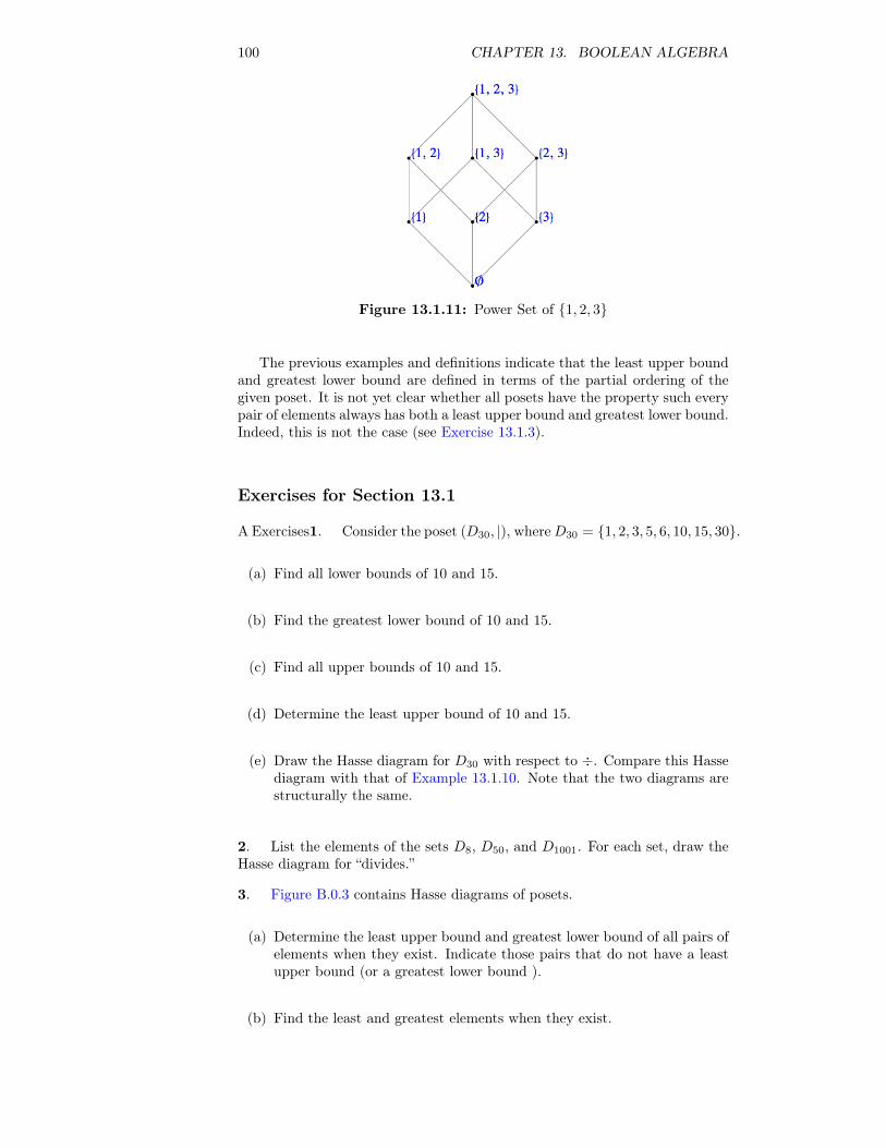
100 CHAPTER 13. BOOLEAN ALGEBRA
Figure 13.1.11: Power Set of {1, 2, 3}
The previous examples and definitions indicate that the least upper boundand greatest lower bound are defined in terms of the partial ordering of thegiven poset. It is not yet clear whether all posets have the property such everypair of elements always has both a least upper bound and greatest lower bound.Indeed, this is not the case (see Exercise 13.1.3).
Exercises for Section 13.1
A Exercises1. Consider the poset (D30, |), whereD30 = {1, 2, 3, 5, 6, 10, 15, 30}.
(a) Find all lower bounds of 10 and 15.
(b) Find the greatest lower bound of 10 and 15.
(c) Find all upper bounds of 10 and 15.
(d) Determine the least upper bound of 10 and 15.
(e) Draw the Hasse diagram for D30 with respect to ÷. Compare this Hassediagram with that of Example 13.1.10. Note that the two diagrams arestructurally the same.
2. List the elements of the sets D8, D50, and D1001. For each set, draw theHasse diagram for “divides.”
3. Figure B.0.3 contains Hasse diagrams of posets.
(a) Determine the least upper bound and greatest lower bound of all pairs ofelements when they exist. Indicate those pairs that do not have a leastupper bound (or a greatest lower bound ).
(b) Find the least and greatest elements when they exist.
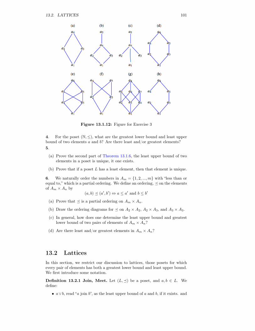
13.2. LATTICES 101
Figure 13.1.12: Figure for Exercise 3
4. For the poset (N,≤), what are the greatest lower bound and least upperbound of two elements a and b? Are there least and/or greatest elements?5.
(a) Prove the second part of Theorem 13.1.6, the least upper bound of twoelements in a poset is unique, it one exists.
(b) Prove that if a poset L has a least element, then that element is unique.
6. We naturally order the numbers in Am = {1, 2, ...,m} with “less than orequal to,” which is a partial ordering. We define an ordering, � on the elementsof Am ×An by
(a, b) � (a′, b′)⇔ a ≤ a′ and b ≤ b′
(a) Prove that � is a partial ordering on Am ×An.
(b) Draw the ordering diagrams for � on A2 ×A2, A2 ×A3, and A3 ×A3.
(c) In general, how does one determine the least upper bound and greatestlower bound of two pairs of elements of Am ×An?
(d) Are there least and/or greatest elements in Am ×An?
13.2 LatticesIn this section, we restrict our discussion to lattices, those posets for whichevery pair of elements has both a greatest lower bound and least upper bound.We first introduce some notation.
Definition 13.2.1 Join, Meet. Let (L,�) be a poset, and a, b ∈ L. Wedefine:
• a∨b, read “a join b”, as the least upper bound of a and b, if it exists. and
102 CHAPTER 13. BOOLEAN ALGEBRA
• a∧ b, read “a meet b”, as the greatest lower bound of a and b, if it exists.
Since the join and meet produce a unique result in all cases where theyexist, by Theorem 13.1.6, we can consider them as binary operations on a setif they always exist. Thus the following definition:
Definition 13.2.2 Lattice. A lattice is a poset (L,�) for which every pair ofelements has a greatest lower bound and least upper bound. Since a lattice L isan algebraic system with binary operations ∨ and ∧, it is denoted by [L;∨,∧].If we want to make it clear what partial ordering the lattice is based on, wesay it is a lattice under �
Example 13.2.3 The power set of a three element set. Consider theposet (P(A),⊆) we examined in Example 13.1.10. It isn’t too surprising thatevery pair of sets had a greatest lower bound and least upper bound. Thus,we have a lattice in this case; and A ∨ B = A ∪ B and A ∧ B = A ∩ B. Thereader is encouraged to write out the operation tables [P(A);∪,∩].
Our first concrete lattice can be generalized to the case of any set A, pro-ducing the lattice [P(A);∨,∧], where the join operation is the set operation ofunion and the meet operation is the operation intersection; that is, ∨ = ∪ and∧ = ∩.
It can be shown (see the exercises) that the commutative laws, associativelaws, idempotent laws, and absorption laws are all true for any lattice. A con-crete example of this is clearly [P(A);∪,∩], since these laws hold in the algebraof sets. This lattice also has distributive property in that join is distributiveover meet and meet is distributive over join. However, this is not always thecase for lattices in general.
Definition 13.2.4 Distributive Lattice. Let L = [L;∨,∧] be a lattice under≤. L is called a distributive lattice if and only if the distributive laws hold;that is, for all a, b, c ∈ L we have
a ∨ (b ∧ c) = (a ∨ b) ∧ (a ∨ c)and
a ∧ (b ∨ c) = (a ∧ b) ∨ (a ∧ c)
Example 13.2.5 A Nondistributive Lattice. We now give an example ofa lattice where the distributive laws do not hold. Let L = {000, a, b, c,111}. Wedefine the partial ordering � on L by the set
{(000,000), (000, a), (000, b), (000, c), (000,111), (a, a), (a,111), (b, b), (b,111), (c, c), (c,111), (111,111)}
The operation tables for ∨ and ∧ on L are:
∨ 000 a b c 111
000 000 a b c 111
a a a 111 111 111
b b 111 b 111 111
c c 111 111 c 111
111 111 111 111 111 111
∧ 000 a b c 111
000 000 000 000 000 000
a 000 a 000 000 a
b 000 000 b 000 b
c 000 000 000 c c
111 000 a b c 111
Since every pair of elements in L has both a join and a meet, [L;∨,∧] is alattice (under divides). Is this lattice distributive? We note that: a∨ (c∧ b) =a∨000 = a and (a∨c)∧(a∨b) = 111∧111 = 111. Therefore, a∨(b∧c) 6= (a∨b)∧(a∨c)for some values of a, b, c ∈ L. Thus, this lattice is not distributive.
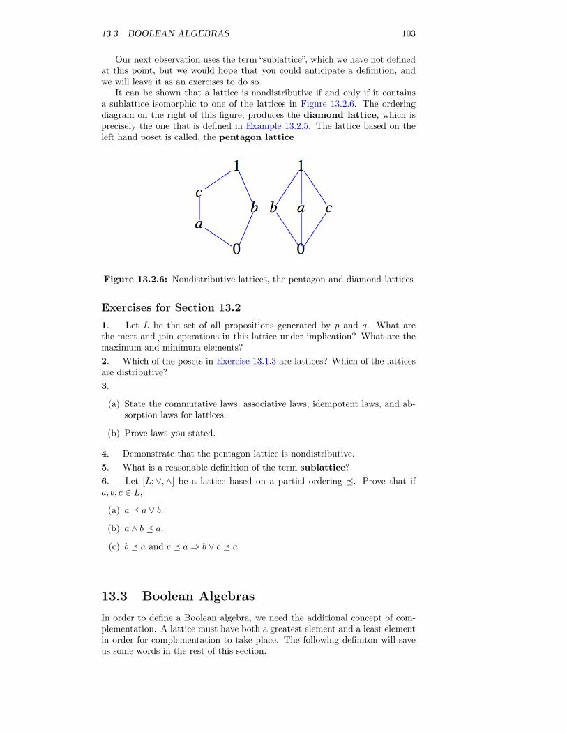
13.3. BOOLEAN ALGEBRAS 103
Our next observation uses the term “sublattice”, which we have not definedat this point, but we would hope that you could anticipate a definition, andwe will leave it as an exercises to do so.
It can be shown that a lattice is nondistributive if and only if it containsa sublattice isomorphic to one of the lattices in Figure 13.2.6. The orderingdiagram on the right of this figure, produces the diamond lattice, which isprecisely the one that is defined in Example 13.2.5. The lattice based on theleft hand poset is called, the pentagon lattice
Figure 13.2.6: Nondistributive lattices, the pentagon and diamond lattices
Exercises for Section 13.21. Let L be the set of all propositions generated by p and q. What arethe meet and join operations in this lattice under implication? What are themaximum and minimum elements?2. Which of the posets in Exercise 13.1.3 are lattices? Which of the latticesare distributive?3.
(a) State the commutative laws, associative laws, idempotent laws, and ab-sorption laws for lattices.
(b) Prove laws you stated.
4. Demonstrate that the pentagon lattice is nondistributive.5. What is a reasonable definition of the term sublattice?6. Let [L;∨,∧] be a lattice based on a partial ordering �. Prove that ifa, b, c ∈ L,
(a) a � a ∨ b.
(b) a ∧ b � a.
(c) b � a and c � a⇒ b ∨ c � a.
13.3 Boolean AlgebrasIn order to define a Boolean algebra, we need the additional concept of com-plementation. A lattice must have both a greatest element and a least elementin order for complementation to take place. The following definiton will saveus some words in the rest of this section.
104 CHAPTER 13. BOOLEAN ALGEBRA
Definition 13.3.1 Bounded Lattice. A bounded lattice is a lattice thatcontains both a least element and a greatest element.
We use the symbols 000 and 111 for the least and greatest elements of a boundedlattice in the remainder of this section.
Definition 13.3.2 The Complement of a Lattice Element. Let [L;∨,∧]be a bounded lattice. If a ∈ L, then a has a complement if there exists b ∈ Lsuch that
a ∨ b = 111
and
a ∧ b = 000
Notice that by the commutative laws for lattices, if b complements a, thena complements b.
Definition 13.3.3 Complemented Lattice. Let L = [L;∨,∧] be a boundedlattice. L is a complemented lattice if every element of L has a complement inL.
Example 13.3.4 Set Complement is a Complement. In Chapter 1, wedefined the complement of a subset of any universe. This turns out to be aconcrete example of the general concept we have just defined, but we will reasonthrough why this is the case here. Let L = P(A), where A = {a, b, c}. Then[L;∪,∩] is a bounded lattice with 0 = ∅ and 1 = A. To find the complement,if it exists, of B = {a, b} ∈ L, for example, we want D such that
{a, b} ∩D = ∅and
{a, b} ∪D = A
It’s not too difficult to see that D = {c}, since we need to include c to makethe first condition true and can’t include a or b if the second condition is to betrue. Of course this is precisely how we defined Ac in Chapter 1. Since it canbe shown that each element of L has a complement (see Exercise 1), [L;∪,∩] isa complemented lattice. Note that if A is any set and L = P(A), then [L;∪,∩]is a complemented lattice where the complement of B ∈ L is Bc = A−B.
In Example 13.3.4, we observed that the complement of each element of Lis unique. Is this always true in a complemented lattice? The answer is no.Consider the following.
Example 13.3.5 A Lattice for which complements are not unique.Let L = {1, 2, 3, 5, 30} and consider the lattice [L;∨,∧] (under “divides”). Theleast element of L is 1 and the greatest element is 30. Let us compute thecomplement of the element a = 2. We want to determine a such that 2∧ a = 1and 2 ∨ a = 30. Certainly, a = 3 works, but so does a = 5, so the complementof a = 2 in this lattice is not unique. However, [L;∨,∧] is still a complementedlattice since each element does have at least one complement.
Definition 13.3.6 Complementation as an operation. If a complementedlattice has the property that the complement of every element is unique, thenwe consider complementation to be a unary operation. The usual notation forthe complement of a is a.
The following theorem gives us an insight into when uniqueness of comple-ments occurs.
13.3. BOOLEAN ALGEBRAS 105
Theorem 13.3.7 One condition for unique complements. If [L;∨,∧]is a complemented, distributive lattice, then the complement of each elementa ∈ L is unique.
Proof. Let a ∈ L and assume to the contrary that a has two complements,namely a1 and a2. Then by the definition of complement,
a ∧ a1 = 0 and a ∨ a1 = 1,
and
a ∧ a2 = 0 and a ∨ a2 = 1,
.
Then
a1 = a1 ∧ 111 = a1 ∧ (a ∨ a2)
= (a1 ∧ a) ∨ (a1 ∧ a2)
= 000 ∨ (a1 ∧ a2)
= a1 ∧ a2
On the other hand,
a2 = a2 ∧ 111 = a2 ∧ (a ∨ a1)
= (a2 ∧ a) ∨ (a2 ∧ a1)
= 000 ∨ (a2 ∧ a1)
= a2 ∧ a1
= a1 ∧ a2
Hence a1 = a2, which contradicts the assumption that a has two differentcomplements.
Definition 13.3.8 Boolean Algebra. A Boolean algebra is a lattice thatcontains a least element and a greatest element and that is both complementedand distributive. The notation [B;∨,∧, ¯ ] is used to denote the booleanalgebra with operations disjunction, conjuction and complementation.
Since the complement of each element in a Boolean algebra is unique (byTheorem 13.3.7), complementation is a valid unary operation over the set underdiscussion, which is why we will list it together with the other two operationsto emphasize that we are discussing a set together with three operations. Also,to help emphasize the distinction between lattices and lattices that are Booleanalgebras, we will use the letter B as the generic symbol for the set of a Booleanalgebra; that is, [B;∨,∧, ¯ ] will stand for a general Boolean algebra.
Example 13.3.9 Boolean Algebra of Sets. Let A be any set, and letB = P(A). Then [B;∪,∩, c] is a Boolean algebra. Here, c stands for thecomplement of an element of B with respect to A, A−B.
This is a key example for us since all finite Boolean algebras and manyinfinite Boolean algebras look like this example for some A. In fact, a glanceat the basic Boolean algebra laws in Table 13.3.11, in comparison with the setlaws of Chapter 4 and the basic laws of logic of Chapter 3, indicates that allthree systems behave the same; that is, they are isomorphic.
Example 13.3.10 Divisors of 30. A somewhat less standard example of aboolean algebra is derived from the lattice of divisors of 30 under the relation
106 CHAPTER 13. BOOLEAN ALGEBRA
“divides”. If you examine the ordering diagram for this lattice, you see that itis structurally the same as the boolean algebra of subsets of a three elementset. Therefore, the join, meet and complementation operations act the sameas union, intersection and set complementation. We might conjecture that thelattice of divisors of any integer will produce a boolean algebra, but it only thecase of certain integers. Try out a few integers to see if you can identify whatis necessary to produce a boolean algebra.
Commutative Laws a ∨ b = b ∨ a a ∧ b = b ∧ aAssociative Laws a ∨ (b ∨ c) = (a ∨ b) ∨ c a ∧ (b ∧ c) = (a ∧ b) ∧ cDistributive Laws a ∧ (b ∨ c) = (a ∧ b) ∨ (a ∧ c) a ∨ (b ∧ c) = (a ∨ b) ∧ (a ∨ c)Identity Laws a ∨ 0 = 0 ∨ a = a a ∧ 1 = 1 ∧ a = a
Complement Laws a ∨ a = 1 a ∧ a = 0
Idempotent Laws a ∨ a = a a ∧ a = a
Null Laws a ∨ 1 = 1 a ∧ 0 = 0
Absorption Laws a ∨ (a ∧ b) = a a ∧ (a ∨ b) = a
DeMorgan’s Laws a ∨ b = a ∧ b a ∧ b = a ∨ bInvolution Law a = a
Table 13.3.11: Basic Boolean Algebra Laws
The “pairings” of the boolean algebra laws reminds us of the principle ofduality, which we state for a Boolean algebra.
Definition 13.3.12 Principle of Duality for Boolean Algebras. Let B =[B;∨,∧, c] be a Boolean algebra under �, and let S be a true statement for B.If S∗ is obtained from S by replacing � with � (this is equivalent to turningthe graph upside down), ∨ with ∧, ∧ with ∨, 000 with 111, and 111 with 000, then S∗is also a true statement in B.
Exercises for Section 13.31. Determine the complement of each element B ∈ L in Example 13.3.4. Isthis lattice a Boolean algebra? Why?2.
(a) Determine the complement of each element of D6 in [D6;∨,∧].
(b) Repeat part a using the lattice in Example 13.2.5.
(c) Repeat part a using the lattice in Exercise 13.1.1.
(d) Are the lattices in parts a, b, and c Boolean algebras? Why?
3. Determine which of the lattices of Exercise 13.1.3 of Section 13.1 areBoolean algebras.4. Let A = {a, b} and B = P(A).
(a) Prove that [B;∪,∩, c] is a Boolean algebra.
(b) Write out the operation tables for the Boolean algebra.
5. It can be shown that the following statement, S, holds for any Booleanalgebra [B;∨,∧,−] : (a ∧ b) = a if and only if a ≤ b.
(a) Write the dual, S∗, of the statement S.
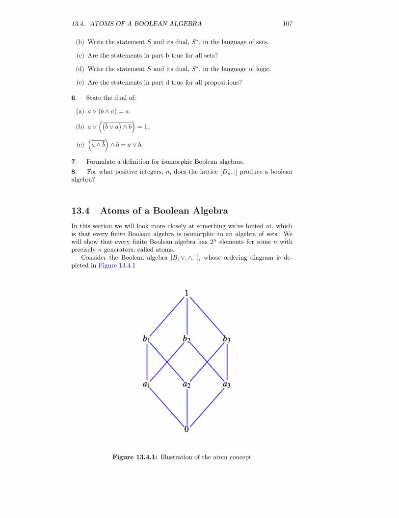
13.4. ATOMS OF A BOOLEAN ALGEBRA 107
(b) Write the statement S and its dual, S∗, in the language of sets.
(c) Are the statements in part b true for all sets?
(d) Write the statement S and its dual, S∗, in the language of logic.
(e) Are the statements in part d true for all propositions?
6. State the dual of:
(a) a ∨ (b ∧ a) = a.
(b) a ∨((b ∨ a
)∧ b)
= 1.
(c)(a ∧ b
)∧ b = a ∨ b.
7. Formulate a definition for isomorphic Boolean algebras.8. For what positive integers, n, does the lattice [Dn, |] produce a booleanalgebra?
13.4 Atoms of a Boolean Algebra
In this section we will look more closely at something we’ve hinted at, whichis that every finite Boolean algebra is isomorphic to an algebra of sets. Wewill show that every finite Boolean algebra has 2n elements for some n withprecisely n generators, called atoms.
Consider the Boolean algebra [B;∨,∧, ], whose ordering diagram is de-picted in Figure 13.4.1
Figure 13.4.1: Illustration of the atom concept
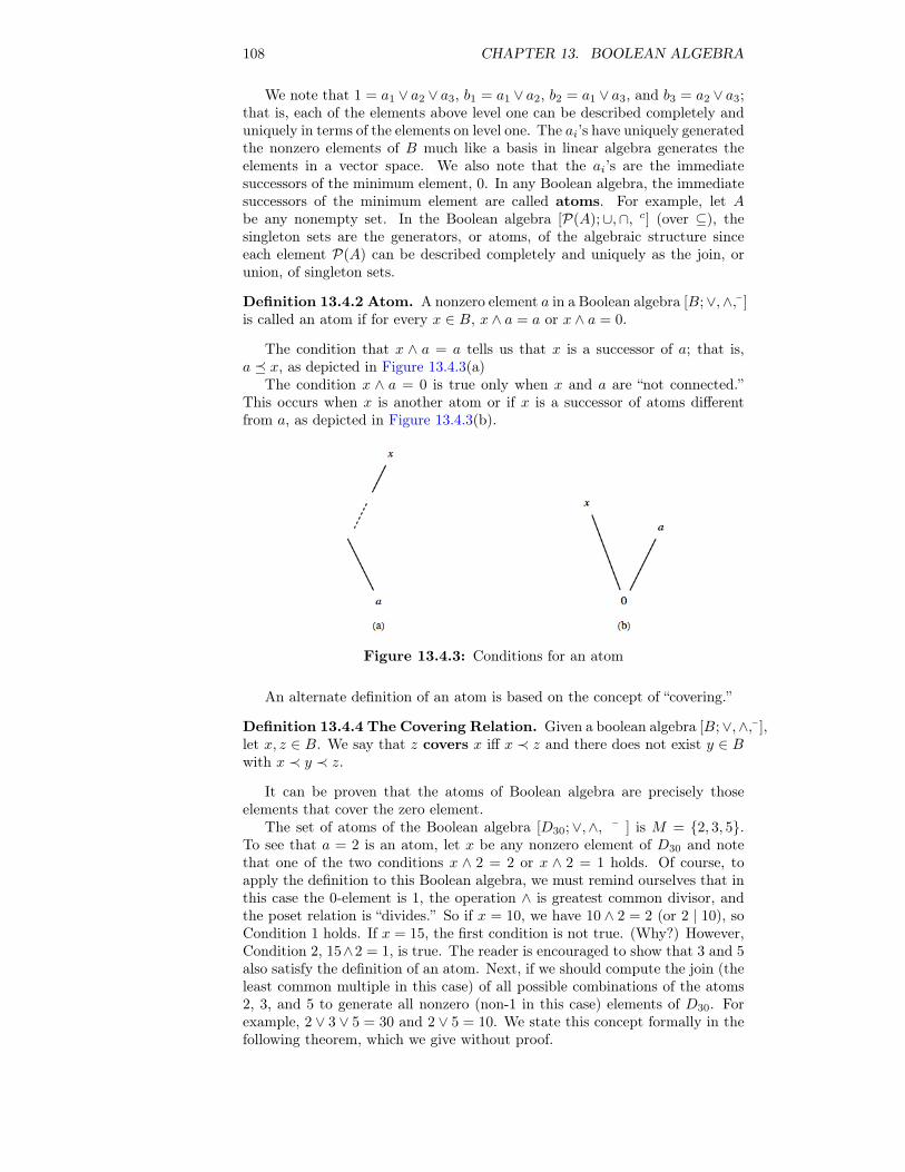
108 CHAPTER 13. BOOLEAN ALGEBRA
We note that 1 = a1 ∨ a2 ∨ a3, b1 = a1 ∨ a2, b2 = a1 ∨ a3, and b3 = a2 ∨ a3;that is, each of the elements above level one can be described completely anduniquely in terms of the elements on level one. The ai’s have uniquely generatedthe nonzero elements of B much like a basis in linear algebra generates theelements in a vector space. We also note that the ai’s are the immediatesuccessors of the minimum element, 0. In any Boolean algebra, the immediatesuccessors of the minimum element are called atoms. For example, let Abe any nonempty set. In the Boolean algebra [P(A);∪,∩, c] (over ⊆), thesingleton sets are the generators, or atoms, of the algebraic structure sinceeach element P(A) can be described completely and uniquely as the join, orunion, of singleton sets.
Definition 13.4.2 Atom. A nonzero element a in a Boolean algebra [B;∨,∧, ]is called an atom if for every x ∈ B, x ∧ a = a or x ∧ a = 0.
The condition that x ∧ a = a tells us that x is a successor of a; that is,a � x, as depicted in Figure 13.4.3(a)
The condition x ∧ a = 0 is true only when x and a are “not connected.”This occurs when x is another atom or if x is a successor of atoms differentfrom a, as depicted in Figure 13.4.3(b).
Figure 13.4.3: Conditions for an atom
An alternate definition of an atom is based on the concept of “covering.”
Definition 13.4.4 The Covering Relation. Given a boolean algebra [B;∨,∧, ],let x, z ∈ B. We say that z covers x iff x ≺ z and there does not exist y ∈ Bwith x ≺ y ≺ z.
It can be proven that the atoms of Boolean algebra are precisely thoseelements that cover the zero element.
The set of atoms of the Boolean algebra [D30;∨,∧, ¯ ] is M = {2, 3, 5}.To see that a = 2 is an atom, let x be any nonzero element of D30 and notethat one of the two conditions x ∧ 2 = 2 or x ∧ 2 = 1 holds. Of course, toapply the definition to this Boolean algebra, we must remind ourselves that inthis case the 0-element is 1, the operation ∧ is greatest common divisor, andthe poset relation is “divides.” So if x = 10, we have 10 ∧ 2 = 2 (or 2 | 10), soCondition 1 holds. If x = 15, the first condition is not true. (Why?) However,Condition 2, 15∧2 = 1, is true. The reader is encouraged to show that 3 and 5also satisfy the definition of an atom. Next, if we should compute the join (theleast common multiple in this case) of all possible combinations of the atoms2, 3, and 5 to generate all nonzero (non-1 in this case) elements of D30. Forexample, 2 ∨ 3 ∨ 5 = 30 and 2 ∨ 5 = 10. We state this concept formally in thefollowing theorem, which we give without proof.
13.4. ATOMS OF A BOOLEAN ALGEBRA 109
Theorem 13.4.5. Let B = [B;∨,∧, ¯] be any finite Boolean algebra. Let A ={a1, a2, . . . , an} be the set of all atoms of B. Then every nonzero element in Bcan be expressed uniquely as the join of a subset of A.
We now ask ourselves if we can be more definitive about the structureof different Boolean algebras of a given order. Certainly, the Boolean alge-bras [D30;∨,∧,∧ ¯ ] and [P(A);∪,∩, c] have the same graph (that of Fig-ure 13.4.1), the same number of atoms, and, in all respects, look the same ex-cept for the names of the elements and the operations. In fact, when we applycorresponding operations to corresponding elements, we obtain correspondingresults. We know from Chapter 11 that this means that the two structures areisomorphic as Boolean algebras. Furthermore, the graphs of these examplesare exactly the same as that of Figure 13.4.1, which is an arbitrary Booleanalgebra of order 8 = 23.
In these examples of a Boolean algebra of order 8, we note that eachhad 3 atoms and 23 = 8 number of elements, and all were isomorphic to[P(A);∪,∩, c], where A = {a, b, c}. This leads us to the following questions:
• Are there any different (nonisomorphic) Boolean algebras of order 8?
• What is the relationship, if any, between finite Boolean algebras and theiratoms?
• How many different (nonisomorphic) Boolean algebras are there of order2? Order 3? Order 4? etc.
The answers to these questions are given in the following theorem andcorollaries.
Theorem 13.4.6. Let B = [B;∨,∧,−] be any finite Boolean algebra, and letA be the set of all atoms of B. Then [P(A);∪,∩, c] is isomorphic to [B;∨,∧,−]
Proof. An isomorphism that serves to prove this theorem is T : P(A) → Bdefined by T (S) =
∨a∈S a, where T (∅) is interpreted as the zero of B. We
leave it to the reader to prove that this is indeed an isomorphism.
Corollary 13.4.7. Every finite Boolean algebra B = [B;∨,∧, ¯ ] has 2n ele-ments for some positive integer n.
Proof. Let A be the set of all atoms of B and let |A| = n. Then there areexactly 2n elements (subsets) in P(A),and by Theorem 13.4.6, [B;−,∨,∧] isisomorphic to [P(A);∪,∩ c] and must also have 2n elements.
Corollary 13.4.8. All Boolean algebras of order 2n are isomorphic to oneanother.
Proof.
Figure 13.4.9: Isomorphisms to be combined
110 CHAPTER 13. BOOLEAN ALGEBRA
Every Boolean algebra of order 2n is isomorphic to [P(A);∪,∩, c] when|A| = n. Hence, if B1 and B2 each have 2n elements, they each have n atoms.Suppose their sets of atoms are A1 and A2, respectively. We know thereare isomorphisms T1 and T2, where Ti : Bi → P(Ai), i = 1, 2. In additionwe have an isomorphism, N from P(A1) into P(A2), which we ask you toprove in Exercise 13.4.9. We can combine these isomorphisms to produce theisomorphism T−1
2 ◦N ◦ T1 : B1 → B2, which proves the corollary.
The above theorem and corollaries tell us that we can only have finiteBoolean algebras of orders 21, 22, 23, .., 2n, and that all finite Boolean algebrasof any given order are isomorphic. These are powerful tools in determining thestructure of finite Boolean algebras. In the next section, we will discuss one ofthe easiest ways of describing a Boolean algebra of any given order.
Exercises for Section 13.4
1.
(a) Show that a = 2 is an atom of the Boolean algebra [D30;∨,∧,−].
(b) Repeat part a for the elements 3 and 5 of D30.
(c) Verify Theorem Theorem 13.4.5 for the Boolean algebra [D30;∨,∧,−].
2. Let A = {a, b, c}.
(a) Rewrite the definition of atom for [P(A);∪,∩, c]. What does a ≤ x meanin this example?
(b) Find all atoms of [P(A);∪,∩, c].
(c) Verify Theorem 13.4.5 for [P(A); c,∪,∩].
3. Verify Theorem 13.4.6 and its corollaries for the Boolean algebras inExercises 1 and 2 of this section.
4. Give an example of a Boolean algebra of order 16 whose elements arecertain subsets of the set 1, 2, 3, 4, 5, 6, 7
5. Corollary 13.4.7 implies that there do not exist Boolean algebras of orders3, 5, 6, 7, 9, etc. (orders different from 2n). Without this corollary, directlyshow that we cannot have a Boolean algebra of order 3.
Hint. Assume that [B;∨,∧,−] is a Boolean algebra of order 3 where B ={0, x, 1} and show that this cannot happen by investigating the possibilitiesfor its operation tables.
6.
(a) There are many different, yet isomorphic, Boolean algebras with twoelements. Describe one such Boolean algebra that is derived from apower set, P(A), under ⊆. Describe a second that is described from Dn,for some n ∈ P , under “divides.”
(b) Since the elements of a two-element Boolean algebra must be the greatestand least elements, 1 and 0, the tables for the operations on {0, 1} aredetermined by the Boolean algebra laws. Write out the operation tablesfor [{0, 1};∨,∧,−].
13.5. FINITE BOOLEAN ALGEBRAS AS N -TUPLES OF 0’S AND 1’S111
7. Find a Boolean algebra with a countably infinite number of elements.8. Prove that the direct product of two Boolean algebras is a Booleanalgebra.Hint. “Copy” the corresponding proof for groups in Section 11.6.9. Prove if two finite setsA1 andA2 both have n elements then [P(A1);∪,∩, c]is isomorphic to [P(A2);∪,∩, c]10. Prove an element of a Boolean algebra is an atom if and only if it coversthe zero element.
13.5 Finite Boolean Algebras as n-tuples of 0’sand 1’s
From the previous section we know that all finite Boolean algebras are oforder 2n, where n is the number of atoms in the algebra. We can thereforecompletely describe every finite Boolean algebra by the algebra of power sets.Is there a more convenient, or at least an alternate way, of defining finiteBoolean algebras? In Chapter 11 we found that we could produce new groupsby taking Cartesian products of previously known groups. We imitate thisprocess for Boolean algebras.
The simplest nontrivial Boolean algebra is the Boolean algebra on the setB2 = {0, 1}. The ordering on B2 is the natural one, 0 ≤ 0, 0 ≤ 1, 1 ≤ 1. If wetreat 0 and 1 as the truth values “false” and “true,” respectively, we see thatthe Boolean operations ∨(join) and ∧(meet) are nothing more than the logicaloperation with the same symbols. The Boolean operation, −, (complementa-tion) is the logical ¬ (negation). In fact, this is why these symbols were chosenas the names of the Boolean operations. The operation tables for [B2;∨,∧,−]are simply those of “or,” “and,” and “not,” which we repeat here.
∨ 0 1
0 0 1
1 1 1
∧ 0 1
0 0 0
1 0 1
u−u
0 1
1 0
By Theorem 13.4.6 and its corollaries, all Boolean algebras of order 2 areisomorphic to this one.
We know that if we formB2×B2 = B22 we obtain the set {(0, 0), (0, 1), (1, 0), (1, 1)},
a set of order 4. We define operations on B22 the natural way, namely com-
ponentwise, so that (0, 1) ∨ (1, 1) = (0 ∨ 1, 1 ∨ 1) = (1, 1), (0, 1) ∧ (1, 1) =(0∧1, 1∧1) = (0, 1) and (0, 1) = (0, 1) = (1, 0). We claim that B2
2 is a Booleanalgebra under the componentwise operations. Hence,
[B2
2 ;∨,∧,]is a Boolean
algebra of order 4. Since all Boolean algebras of order 4 are isomorphic to oneother, we have found a simple way of describing all Boolean algebras of order4.
It is quite clear that we can describe any Boolean algebra of order 8 byconsidering B2 × B2 × B2 = B3
2 and, more generally, any Boolean algebra oforder 2n with Bn2 = B2 ×B2 × · · · ×B2 (n factors).
Exercises for Section 13.5
1.
(a) Write out the operation tables for[B2
2 ;∨,∧,−].
112 CHAPTER 13. BOOLEAN ALGEBRA
(b) Draw the Hasse diagram for[B2
2 ;∨,∧,−]and compare your results with
Figure 6.0.1.
(c) Find the atoms of this Boolean algebra.
2.
(a) Write out the operation tables for[B3
2 ;∨,∧,−].
(b) Draw the Hasse diagram for[B3
2 ;∨,∧,−]
3.
(a) List all atoms of B42 .
(b) Describe the atoms of Bn2 , n ≥ 1.
4. Theorem 13.4.6 tells us we can think of any finite Boolean algebra interms of sets. In Chapter 4, we defined minsets 4.0.1 and minset normalform 4.0.2. Rephrase these definitions in the language of Boolean algebra.The generalization of minsets are called minterms.
13.6 Boolean Expressions
In this section, we will use our background from the previous sections and settheory to develop a procedure for simplifying Boolean expressions. This proce-dure has considerable application to the simplification of circuits in switchingtheory or logical design.
Definition 13.6.1 Boolean Expression. Let [B;∨,∧,−] be any Booleanalgebra, and let x1, x2, . . . , xk be variables in B; that is, variables that canassume values from B. A Boolean expression generated by x1, x2, . . . , xk isany valid combination of the xi and the elements of B with the operations ofmeet, join, and complementation.
This definition is the analog of the definition of a proposition generated bya set of propositions, presented in Section 3.2.
Each Boolean expression generated by k variables, e (x1, . . . , xk), definesa function f : Bk → B where f (a1, . . . , ak) = e (a1, . . . , ak). If B is a finiteBoolean algebra, then there are a finite number of functions from Bk into B.Those functions that are defined in terms of Boolean expressions are calledBoolean functions. As we will see, there is an infinite number of Booleanexpressions that define each Boolean function. Naturally, the “shortest” ofthese expressions will be preferred. Since electronic circuits can be describedas Boolean functions with B = B2, this economization is quite useful.
In what follows, we make use of Exercise 7.7 in Section 7.1 for countingnumber of functions.
Example 13.6.2 Two variables over B2. Consider any Boolean algebraof order 2, [B;∨,∧,−]. How many functions f : B2 → B are there? First,all Boolean algebras of order 2 are isomorphic to [B2;∨,∧,−] so we want todetermine the number of functions f : B2
2 → B2. If we consider a Booleanfunction of two variables, x1 and x2, we note that each variable has two possiblevalues 0 and 1, so there are 22 ways of assigning these two values to the k = 2
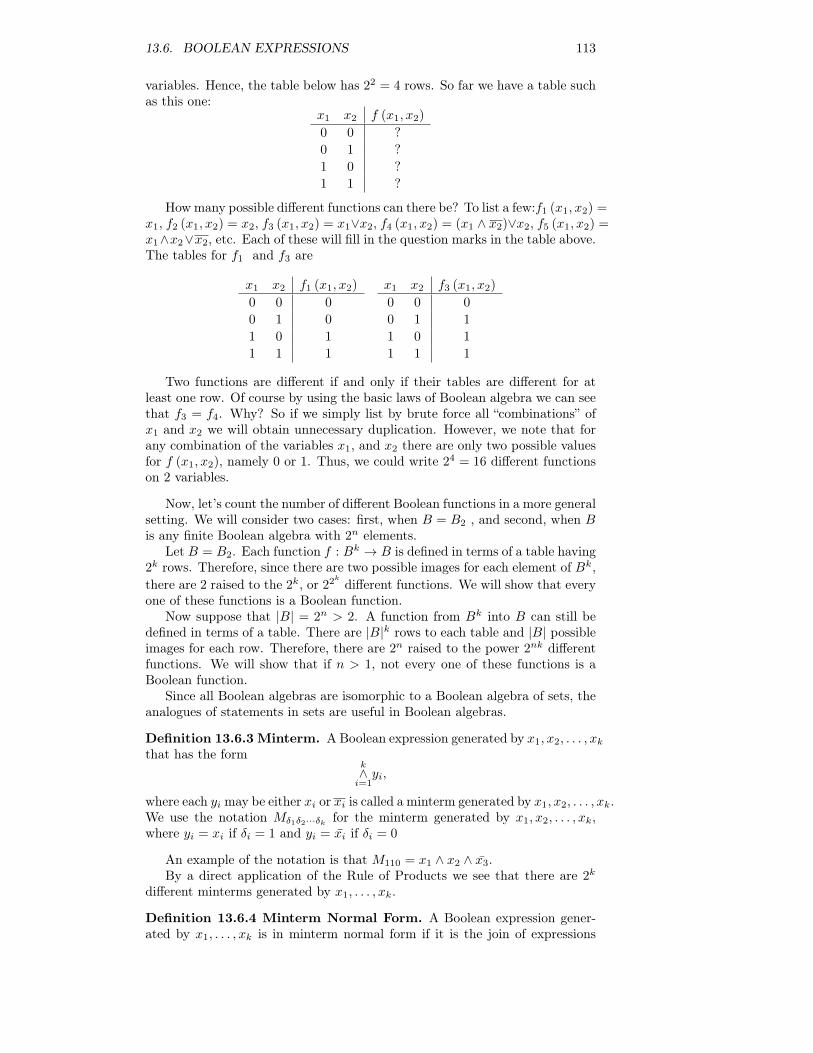
13.6. BOOLEAN EXPRESSIONS 113
variables. Hence, the table below has 22 = 4 rows. So far we have a table suchas this one:
x1 x2 f (x1, x2)
0 0 ?
0 1 ?
1 0 ?
1 1 ?
Howmany possible different functions can there be? To list a few:f1 (x1, x2) =x1, f2 (x1, x2) = x2, f3 (x1, x2) = x1∨x2, f4 (x1, x2) = (x1 ∧ x2)∨x2, f5 (x1, x2) =x1∧x2∨x2, etc. Each of these will fill in the question marks in the table above.The tables for f1 and f3 are
x1 x2 f1 (x1, x2)
0 0 0
0 1 0
1 0 1
1 1 1
x1 x2 f3 (x1, x2)
0 0 0
0 1 1
1 0 1
1 1 1
Two functions are different if and only if their tables are different for atleast one row. Of course by using the basic laws of Boolean algebra we can seethat f3 = f4. Why? So if we simply list by brute force all “combinations” ofx1 and x2 we will obtain unnecessary duplication. However, we note that forany combination of the variables x1, and x2 there are only two possible valuesfor f (x1, x2), namely 0 or 1. Thus, we could write 24 = 16 different functionson 2 variables.
Now, let’s count the number of different Boolean functions in a more generalsetting. We will consider two cases: first, when B = B2 , and second, when Bis any finite Boolean algebra with 2n elements.
Let B = B2. Each function f : Bk → B is defined in terms of a table having2k rows. Therefore, since there are two possible images for each element of Bk,there are 2 raised to the 2k, or 22k
different functions. We will show that everyone of these functions is a Boolean function.
Now suppose that |B| = 2n > 2. A function from Bk into B can still bedefined in terms of a table. There are |B|k rows to each table and |B| possibleimages for each row. Therefore, there are 2n raised to the power 2nk differentfunctions. We will show that if n > 1, not every one of these functions is aBoolean function.
Since all Boolean algebras are isomorphic to a Boolean algebra of sets, theanalogues of statements in sets are useful in Boolean algebras.
Definition 13.6.3 Minterm. A Boolean expression generated by x1, x2, . . . , xkthat has the form
k∧i=1yi,
where each yi may be either xi or xi is called a minterm generated by x1, x2, . . . , xk.We use the notation Mδ1δ2···δk for the minterm generated by x1, x2, . . . , xk,where yi = xi if δi = 1 and yi = xi if δi = 0
An example of the notation is that M110 = x1 ∧ x2 ∧ x3.By a direct application of the Rule of Products we see that there are 2k
different minterms generated by x1, . . . , xk.
Definition 13.6.4 Minterm Normal Form. A Boolean expression gener-ated by x1, . . . , xk is in minterm normal form if it is the join of expressions
114 CHAPTER 13. BOOLEAN ALGEBRA
of the form a ∧m, where a ∈ B and m is a minterm generated by x1, . . . , xk.That is, it is of the form
p∨j=1
(aj ∧mj) (13.6.1)
where p = 2k, and m1,m2, . . . ,mp are the minterms generated by x1, . . . , xk.
Note 13.6.5.
• We seem to require every minterm generated by x1, . . . , xk, in (13.6.1),and we really do. However, some of the values of aj can be 000, whicheffectively makes the corresponding minterm disappear.
• If B = B2, then each aj in a minterm normal form is either 0 or 1.Therefore, aj ∧mj is either 0 or mj .
Theorem 13.6.6 Uniqueness of Minterm Normal Form. Let e (x1, . . . , xk)be a Boolean expression over B. There exists a unique minterm normal formM (x1, . . . , xk) that is equivalent to e (x1, . . . , xk) in the sense that e and Mdefine the same function from Bk into B.
The uniqueness in this theorem does not include the possible ordering ofthe minterms in M (commonly referred to as “uniqueness up to the orderof minterms”). The proof of this theorem would be quite lengthy, and notvery instructive, so we will leave it to the interested reader to attempt. Theimplications of the theorem are very interesting, however.
If |B| = 2n, then there are 2n raised to the 2k different minterm normalforms. Since each different minterm normal form defines a different function,there are a like number of Boolean functions from Bk into B. If B = B2, thereare as many Boolean functions (2 raised to the 2k) as there are functions fromBk into B, since there are 2 raised to the 2n functions from Bk into B. Thesignificance of this result is that any desired function can be realized usingelectronic circuits having 0 or 1 (off or on, positive or negative) values.
More complex, multivalued circuits corresponding to boolean algebras withmore than two values would not have this flexibility because of the number ofminterm normal forms, and hence the number of boolean functions, is strictlyless than the number of functions.
We will close this section by examining minterm normal forms for expres-sions over B2 , since they are a starting point for circuit economization.
Example 13.6.7. Consider the Boolean expression f (x1, x2) = x1 ∨ x2. Onemethod of determining the minterm normal form of f is to think in termsof sets. Consider the diagram with the usual translation of notation in Fig-ure 13.6.8. Then
f (x1, x2) = (x1 ∧ x2) ∨ (x1 ∧ x2) ∨ (x1 ∧ x2)
= M00 ∨M10 ∨M11
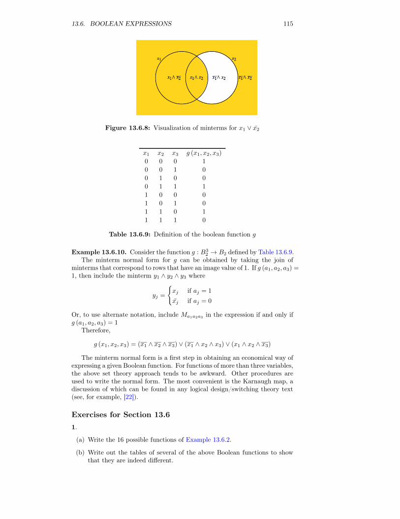
13.6. BOOLEAN EXPRESSIONS 115
Figure 13.6.8: Visualization of minterms for x1 ∨ x2
x1 x2 x3 g (x1, x2, x3)
0 0 0 1
0 0 1 0
0 1 0 0
0 1 1 1
1 0 0 0
1 0 1 0
1 1 0 1
1 1 1 0
Table 13.6.9: Definition of the boolean function g
Example 13.6.10. Consider the function g : B32 → B2 defined by Table 13.6.9.
The minterm normal form for g can be obtained by taking the join ofminterms that correspond to rows that have an image value of 1. If g (a1, a2, a3) =1, then include the minterm y1 ∧ y2 ∧ y3 where
yj =
{xj if aj = 1
xj if aj = 0
Or, to use alternate notation, include Ma1a2a3 in the expression if and only ifg (a1, a2, a3) = 1
Therefore,
g (x1, x2, x3) = (x1 ∧ x2 ∧ x3) ∨ (x1 ∧ x2 ∧ x3) ∨ (x1 ∧ x2 ∧ x3)
The minterm normal form is a first step in obtaining an economical way ofexpressing a given Boolean function. For functions of more than three variables,the above set theory approach tends to be awkward. Other procedures areused to write the normal form. The most convenient is the Karnaugh map, adiscussion of which can be found in any logical design/switching theory text(see, for example, [22]).
Exercises for Section 13.61.
(a) Write the 16 possible functions of Example 13.6.2.
(b) Write out the tables of several of the above Boolean functions to showthat they are indeed different.
116 CHAPTER 13. BOOLEAN ALGEBRA
(c) Determine the minterm normal forms of
(i) g1 (x1, x2) = x1 ∨ x2,
(ii) g2 (x1, x2) = x1 ∨ x2
(iii) g3 (x1, x2) = x1 ∧ x2
(iv) g4 (x1, x2) = 1
2. Consider the Boolean expression f (x1, x2, x3) = (x3 ∧ x2) ∨ (x1 ∧ x3) ∨(x2 ∧ x3) on
[B3
2 ;∨,∧,−].
(a) Simplify this expression using basic Boolean algebra laws.
(b) Write this expression in minterm normal form.
(c) Write out the table for the given function defined by f and compare itto the tables of the functions in parts a and b.
(d) How many possible different functions in three variables on [B2;∨,∧,−]are there?
3. Let [B;∨,∧,−] be a Boolean algebra of order 4, and let f be a Booleanfunction of two variables on B.
(a) How many elements are there in the domain of f?
(b) How many different Boolean functions are there of two, variables? Threevariables?
(c) Determine the minterm normal form of f (x1, x2) = x1 ∨ x2.
(d) If B = {0, a, b, 1}, define a function from B2 into B that is not a Booleanfunction.
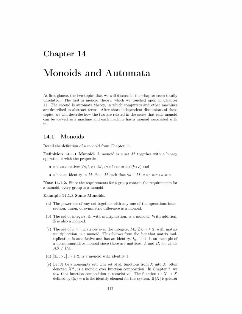
Chapter 14
Monoids and Automata
At first glance, the two topics that we will discuss in this chapter seem totallyunrelated. The first is monoid theory, which we touched upon in Chapter11. The second is automata theory, in which computers and other machinesare described in abstract terms. After short independent discussions of thesetopics, we will describe how the two are related in the sense that each monoidcan be viewed as a machine and each machine has a monoid associated withit.
14.1 MonoidsRecall the definition of a monoid from Chapter 11.
Definition 14.1.1 Monoid. A monoid is a set M together with a binaryoperation ∗ with the properties
• ∗ is associative: ∀a, b, c ∈M , (a ∗ b) ∗ c = a ∗ (b ∗ c) and
• ∗ has an identity in M : ∃e ∈M such that ∀a ∈M , a ∗ e = e ∗ a = a
Note 14.1.2. Since the requirements for a group contain the requirements fora monoid, every group is a monoid.
Example 14.1.3 Some Monoids.
(a) The power set of any set together with any one of the operations inter-section, union, or symmetric difference is a monoid.
(b) The set of integers, Z, with multiplication, is a monoid. With addition,Z is also a monoid.
(c) The set of n × n matrices over the integers, Mn(Z), n ≥ 2, with matrixmultiplication, is a monoid. This follows from the fact that matrix mul-tiplication is associative and has an identity, In. This is an example ofa noncommutative monoid since there are matrices, A and B, for whichAB 6= BA.
(d) [Zn;×n] , n > 2, is a monoid with identity 1.
(e) Let X be a nonempty set. The set of all functions from X into X, oftendenoted XX , is a monoid over function composition. In Chapter 7, wesaw that function composition is associative. The function i : X → Xdefined by i(a) = a is the identity element for this system. If |X| is greater
117
118 CHAPTER 14. MONOIDS AND AUTOMATA
than 1 then it is a noncommutative monoid. If X is finite,∣∣XX
∣∣ = |X||X|. For example, if B = {0, 1},
∣∣BB∣∣ = 4. The functions z, u, i, and t,defined by the graphs in Figure 14.1.4, are the elements of BB . Thismonoid is not a group. Do you know why?
One reason why BB is noncommutative is that t ◦ z 6= z ◦ t because(t ◦ z)(0) = t(z(0)) = t(0) = 1 while (z ◦ t)(0) = z(t(0)) = z(1) = 0.
Figure 14.1.4: The functions on B2
Virtually all of the group concepts that were discussed in Chapter 11 areapplicable to monoids. When we introduced subsystems, we saw that a sub-monoid of monoidM is a subset ofM ; that is, it is a monoid with the operationof M . To prove that a subset is a submonoid, you can apply the following the-orem.
Theorem 14.1.5 Submonoid Test. Assume [M ; ∗] is a monoid and K isa nonempty subset of M . Then K is a submonoid of M if and only if thefollowing two conditions are met.
• If a, b ∈ K, then. a ∗ b ∈ K; i. e., K is closed with under ∗.
• The identity of M belongs to K.
Often we will want to discuss the smallest submonoid that includes a certainsubset S of a monoid M . This submonoid can be defined recursively by thefollowing definition.
Definition 14.1.6 Submonoid Generated by a Set. If S is a subset ofmonoid [M ; ∗], the submonoid generated by S, 〈S〉, is defined by:.
(a) (Basis) The identity of M belongs to 〈S〉; and a ∈ S ⇒ a ∈ 〈S〉.
(b) (Recursion) a, b ∈ 〈S〉 ⇒ a ∗ b ∈ 〈S〉.
Note 14.1.7. If S = {a1, a2, . . . , an}, we write 〈a1, a2, . . . , an〉 in place of〈{a1, a2, . . . , an}〉.
Example 14.1.8 Some Submonoids.
(a) One example of a submonoid of [Z; +] is 〈2〉 = {0, 2, 4, 6, 8, . . .}.
(b) The power set of Z, P(Z), over union is a monoid with identity ∅. IfS = {{1}, {2}, {3}}, then 〈S〉 is the power set of {1, 2, 3}. If S = {{n} :n ∈ Z}, then 〈S〉 is the set of finite subsets of the integers.
14.1. MONOIDS 119
As you might expect, two monoids are isomorphic if and only if there existsa translation rule between them so that any true proposition in one monoid istranslated to a true proposition in the other.
Example 14.1.9. M = [P{1, 2, 3};∩] is isomorphic to M2 =[Z3
2; ·], where
the operation in M2 is componentwise mod 2 multiplication. A translationrule is that if A ⊆ {1, 2, 3}, then it is translated to (d1, d2, d3) where
di =
{1 if i ∈ A0 if i /∈ A
Two cases of how this translation rule works are:
{1, 2, 3} is the identity for M1
l(1, 1, 1) is the identity for M2
{1, 2} ∩ {2, 3} = {2}l
(1, 1, 0) · (0, 1, 1) = (0, 1, 0).
A more precise definition of a monoid isomorphism is identical to the defi-nition of a group isomorphism, Definition 11.7.9.
Exercises for Section 14.1
1. For each of the subsets of the indicated monoid, determine whether thesubset is a submonoid.
(a) S1 = {0, 2, 4, 6} and S2 = {1, 3, 5, 7} in [Z8;×8].
(b) {f ∈ NN : f(n) 6 n,∀n ∈ N} and{f ∈ NN : f(1) = 2
}in the monoid
[NN; ◦].
(c) {A ⊆ Z | A is finite} and {A ⊆ Z | Ac is finite} in [P(Z);∪].
2. For each subset, describe the submonoid that it generates.
(a) {3} in [Z12;×12]
(b) {5} in [Z25;×25]
(c) the set of prime numbers in [P; ·]
(d) {3, 5} in [N; +]
3. An n× n matrix of real numbers is called stochastic if and only if eachentry is nonnegative and the sum of entries in each column is 1. Prove thatthe set of stochastic matrices is a monoid over matrix multiplication.
4. A semigroup is an algebraic system [S; ∗] with the only axiom that ∗be associative on S. Prove that if S is a finite set, then there must exist anidempotent element, that is, an a ∈ S such that a ∗ a = a.
5. Let B be a Boolean algebra and M the set of all Boolean functions onB. Let ∗ be defined on M by (f ∗ g)(a) = f(a) ∧ g(a). Prove that [M ; ∗] is amonoid. Construct the operation table of [M ; ∗] for the case of B = B2.
120 CHAPTER 14. MONOIDS AND AUTOMATA
14.2 Free Monoids and LanguagesIn this section, we will introduce the concept of a language. Languages aresubsets of a certain type of monoid, the free monoid over an alphabet. Afterdefining a free monoid, we will discuss languages and some of the basic problemsrelating to them. We will also discuss the common ways in which languagesare defined.
Let A be a nonempty set, which we will call an alphabet. Our primaryinterest will be in the case where A is finite; however, A could be infinite formost of the situations that we will describe. The elements of A are calledletters or symbols. Among the alphabets that we will use are B = {0, 1},and the set of ASCII (American Standard Code for Information Interchange)characters, which we symbolize as ASCII.
Definition 14.2.1 Strings over an Alphabet. A string of length n, n > 1over alphabet A is a sequence of n letters from A: a1a2 . . . an. The null string,λ, is defined as the string of length zero containing no letters. The set of stringsof length n over A is denoted by An. The set of all strings over A is denotedA∗.
Note 14.2.2.
(a) If the length of string s is n, we write |s| = n.
(b) The null string is not the same as the empty set, although they are similarin many ways. A0 = {λ}.
(c) A∗ = A0 ∪ A1 ∪ A2 ∪ A3 ∪ · · · and if i 6= j, Ai ∩ Aj = ∅; that is,{A0, A1, A2, A3, . . .} is a partition of A∗.
(d) An element of A can appear any number of times in a string.
Theorem 14.2.3. If A is countable, then A∗ is countable.
Proof. Case 1. Given the alphabet B = {0, 1}, we can define a bijec-tion from the positive integers into B∗. Each positive integer has a binaryexpansion dkdk−1 · · · d1d0, where each dj is 0 or 1 and dk = 1. If n hassuch a binary expansion, then 2k ≤ n ≤ 2k+1. We define f : P → B∗ byf(n) = f (dkdk−1 · · · d1d0) = dk−1 · · · d1d0, where f(1) = λ. Every one of the2k strings of length k are the images of exactly one of the integers between2k and 2k+1 − 1. From its definition, f is clearly a bijection; therefore, B∗ iscountable.
Case 2: A is Finite. We will describe how this case is handled with anexample first and then give the general proof. If A = {a, b, c, d, e}, then we cancode the letters in A into strings from B3. One of the coding schemes (thereare many) is a ↔ 000, b ↔ 001, c ↔ 010, d ↔ 011, and e ↔ 100. Now everystring in A∗ corresponds to a different string in B∗; for example, ace. wouldcorrespond with 000010100. The cardinality of A∗ is equal to the cardinality ofthe set of strings that can be obtained from this encoding system. The possiblecoded strings must be countable, since they are a subset of a countable set,B∗. Therefore, A∗ is countable.
If |A| = m, then the letters in A can be coded using a set of fixed-lengthstrings from B∗. If 2k−1 < m ≤ 2k, then there are at least as many strings oflength k in Bk as there are letters in A. Now we can associate each letter in Awith with a different element of Bk. Then any string in A∗. corresponds to astring in B∗. By the same reasoning as in the example above, A∗ is countable.
Case 3: A is Countably Infinite. We will leave this case as an exercise.
14.2. FREE MONOIDS AND LANGUAGES 121
Definition 14.2.4 Concatenation. Let a = a1a2 · · · am and b = b1b2 · · · bnbe strings of length m and n, respectively. The concatenation of a with b, a+b,is the string a1a2 · · · amb1b2 · · · bn of length m+ n.
There are several symbols that are used for concatenation. We chose to usethe one that is also used in Python and SageMath.
'good'+'bye'
'goodbye '
The set of strings over any alphabet is a monoid under concatenation.
Note 14.2.5.
(a) The null string is the identity element of [A∗; +]. Henceforth, we willdenote the monoid of strings over A by A∗.
(b) Concatenation is noncommutative, provided |A| > 1.
(c) If |A1| = |A2|, then the monoids A∗1 and A∗2 are isomorphic. An iso-morphism can be defined using any bijection f : A1 → A2. If a =a1a2 · · · an ∈ A∗1, f∗(a) = (f(a1)f(a2) · · · f(an)) defines a bijection fromA∗1 into A∗2. We will leave it to the reader to prove that for all a, b,∈A∗1, f
∗(a+ b) = f∗(a) + f∗(b).
The languages of the world, English, German, Russian, Chinese, and soforth, are called natural languages. In order to communicate in writing in anyone of them, you must first know the letters of the alphabet and then know howto combine the letters in meaningful ways. A formal language is an abstractionof this situation.
Definition 14.2.6 Formal Language. If A is an alphabet, a formal languageover A is a subset of A∗.
Example 14.2.7 Some Formal Languages.
(a) English can be thought of as a language over of letters A,B, · · ·Z, bothupper and lower case, and other special symbols, such as punctuationmarks and the blank. Exactly what subset of the strings over this alpha-bet defines the English language is difficult to pin down exactly. Thisis a characteristic of natural languages that we try to avoid with formallanguages.
(b) The set of all ASCII stream files can be defined in terms of a languageover ASCII. An ASCII stream file is a sequence of zero or more linesfollowed by an end-of-file symbol. A line is defined as a sequence ofASCII characters that ends with the a “new line” character. The end-of-file symbol is system-dependent.
(c) The set of all syntactically correct expressions in any computer languageis a language over the set of ASCII strings.
(d) A few languages over B are
• L1 = {s ∈ B∗ | s has exactly as many 1’s as it has 0’s}• L2 = {1 + s+ 0 | s ∈ B∗}• L3 = 〈0, 01〉 = the submonoid of B∗ generated by {0, 01}.
122 CHAPTER 14. MONOIDS AND AUTOMATA
Investigation 14.2.1 Two Fundamental Problems: Recognition andGeneration. The generation and recognition problems are basic to computerprogramming. Given a language, L, the programmer must know how to write(or generate) a syntactically correct program that solves a problem. On theother hand, the compiler must be written to recognize whether a programcontains any syntax errors.
Problem 14.2.8 The Recognition Problem. Given a formal language overalphabet A, the Recognition Problem is to design an algorithm that determinesthe truth of s ∈ L in a finite number of steps for all s ∈ A∗. Any such algorithmis called a recognition algorithm.
Definition 14.2.9 Recursive Language. A language is recursive if thereexists a recognition algorithm for it.
Example 14.2.10 Some Recursive Languages.
(a) The language of syntactically correct propositions over set of proposi-tional variables expressions is recursive.
(b) The three languages in 7(d) are all recursive. Recognition algorithms forL1 and L2 should be easy for you to imagine. The reason a recognitionalgorithm for L3 might not be obvious is that the definition of L3 is morecryptic. It doesn’t tell us what belongs to L3, just what can be used tocreate strings in L3. This is how many languages are defined. With asecond description of L3, we can easily design a recognition algorithm.You can prove that
L3 = {s ∈ B∗ | s = λ or s starts with a 0 and has no consecutive 1’s}.
Problem 14.2.11 The Generation Problem. Design an algorithm thatgenerates or produces any string in L. Here we presume that A is either finiteor countably infinite; hence, A∗ is countable by Theorem 14.2.3, and L ⊆ A∗
must be countable. Therefore, the generation of L amounts to creating a listof strings in L. The list may be either finite or infinite, and you must be ableto show that every string in L appears somewhere in the list.
Theorem 14.2.12 Recursive implies Generating.
(a) If A is countable, then there exists a generating algorithm for A∗.
(b) If L is a recursive language over a countable alphabet, then there existsa generating algorithm for L.
Proof. Part (a) follows from the fact that A∗ is countable; therefore, thereexists a complete list of strings in A∗.
To generate all strings of L, start with a list of all strings in A∗ and anempty list, W , of strings in L. For each string s, use a recognition algorithm(one exists since L is recursive) to determine whether s ∈ L. If s ∈ L, add it toW ; otherwise “throw it out.” Then go to the next string in the list of A∗.
Example 14.2.13. Since all of the languages in 7(d) are recursive, they musthave generating algorithms. The one given in the proof of Theorem 14.2.12is not usually the most efficient. You could probably design more efficientgenerating algorithms for L2 and L3; however, a better generating algorithmfor L1 is not quite so obvious.
14.2. FREE MONOIDS AND LANGUAGES 123
The recognition and generation problems can vary in difficulty dependingon how a language is defined and what sort of algorithms we allow ourselvesto use. This is not to say that the means by which a language is defineddetermines whether it is recursive. It just means that the truth of the statement“L is recursive” may be more difficult to determine with one definition thanwith another. We will close this section with a discussion of grammars, whichare standard forms of definition for a language. When we restrict ourselvesto only certain types of algorithms, we can affect our ability to determinewhether s ∈ L is true. In defining a recursive language, we do not restrictourselves in any way in regard to the type of algorithm that will be used. Inthe next section, we will consider machines called finite automata, which canonly perform simple algorithms.
One common way of defining a language is by means of a phrase structuregrammar (or grammar, for short). The set of strings that can be producedusing set of grammar rules is called a phrase structure language.
Example 14.2.14 Zeros before Ones. We can define the set of all stringsover B for which all 0’s precede all 1’s as follows. Define the starting symbolS and establish rules that S can be replaced with any of the following: λ, 0S,or S1. These replacement rules are usually called production rules. They areusually written in the format S → λ, S → 0S, and S → S1. Now define L tobe the set of all strings that can be produced by starting with S and applyingthe production rules until S no longer appears. The strings in L are exactlythe ones that are described above.
Definition 14.2.15 Phrase Structure Grammar. A phrase structure gram-mar consists of four components:
(1) A nonempty finite set of terminal characters, T . If the grammar is defin-ing a language over A, T is a subset of A∗.
(2) A finite set of nonterminal characters, N .
(3) A starting symbol, S ∈ N .
(4) A finite set of production rules, each of the form X → Y , where X andY are strings over A ∪N such that X 6= Y and X contains at least onenonterminal symbol.
If G is a phrase structure grammar, L(G) is the set of strings that can beproduced by starting with S and applying the production rules a finite numberof times until no nonterminal characters remain. If a language can be definedby a phrase structure grammar, then it is called a phrase structure language.
Example 14.2.16 Alternating bits language. The language over B con-sisting of strings of alternating 0’s and 1’s is a phrase structure language. Itcan be defined by the following grammar:
(1) Terminal characters: λ, 0, and 1
(2) Nonterminal characters: S, T , and U
(3) Starting symbol: S
(4) Production rules:
S → T S → U S → λ
S → 0 S → 1
S → 0T S → 1U
T → 10T T → 10
U → 01U U → 01
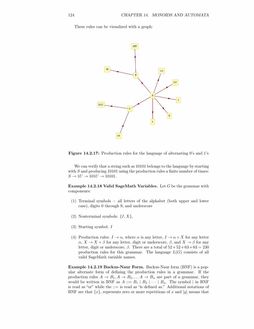
124 CHAPTER 14. MONOIDS AND AUTOMATA
These rules can be visualized with a graph:
Figure 14.2.17: Production rules for the language of alternating 0’s and 1’s
We can verify that a string such as 10101 belongs to the language by startingwith S and producing 10101 using the production rules a finite number of times:S → 1U → 101U → 10101.
Example 14.2.18 Valid SageMath Variables. Let G be the grammar withcomponents:
(1) Terminal symbols = all letters of the alphabet (both upper and lowercase), digits 0 through 9, and underscore
(2) Nonterminal symbols: {I,X},
(3) Starting symbol: I
(4) Production rules: I → α, where α is any letter, I → α+X for any letterα, X → X + β for any letter, digit or underscore, β, and X → β for anyletter, digit or underscore, β. There are a total of 52+52+63+63 = 230production rules for this grammar. The language L(G) consists of allvalid SageMath variable names.
Example 14.2.19 Backus-Naur Form. Backus-Naur form (BNF) is a pop-ular alternate form of defining the production rules in a grammar. If theproduction rules A → B1, A → B2, . . . A → Bn are part of a grammar, theywould be written in BNF as A ::= B1 | B2 | · · · | Bn. The symbol | in BNFis read as “or” while the ::= is read as “is defined as.” Additional notations ofBNF are that {x}, represents zero or more repetitions of x and [y] means that
14.2. FREE MONOIDS AND LANGUAGES 125
y is optional.A BNF version of the production rules for a SageMath variable, I, is
letter ::= a | b | c | · · · | z | A | B | · · · | Zdigit ::= 0 | 1 | · · · | 9I ::= letter{letter | digit | _}
Example 14.2.20 The language of simple arithmetic expressions. Anarithmetic expression can be defined in BNF. For simplicity, we will consideronly expressions obtained using addition and multiplication of integers. Theterminal symbols are (,),+,*, -, and the digits 0 through 9. The nonterminalsymbols are E (for expression), T (term), F (factor), and N (number). Thestarting symbol is E. Production rules are
E: := E + T | TT ::= T ∗ F | FF ::= (E) | N
N ::= [−]digit{digit}.
One particularly simple type of phrase structure grammar is the regulargrammar.
Definition 14.2.21 Regular Grammar. A regular (right-hand form) gram-mar is a grammar whose production rules are all of the form A → t andA→ tB, where A and B are nonterminal and t is terminal. A left-hand formgrammar allows only A→ t and A→ Bt. A language that has a regular phrasestructure language is called a regular language.
Example 14.2.22.
(a) The set of Sage variable names is a regular language since the grammarby which we defined the set is a regular grammar.
(b) The language of all strings for which all 0’s precede all 1’s (Exam-ple 14.2.14) is regular; however, the grammar by which we defined thisset is not regular. Can you define these strings with a regular grammar?
(c) The language of arithmetic expressions is not regular.
Exercises for Section 14.21.
(a) If a computer is being designed to operate with a character set of 350symbols, how many bits must be reserved for each character? Assumeeach character will use the same number of bits.
(b) Do the same for 3,500 symbols.
2. It was pointed out in the text that the null string and the null set aredifferent. The former is a string and the latter is a set, two different kinds ofobjects. Discuss how the two are similar.3. What sets of strings are defined by the following grammar?
(a) Terminal symbols: λ , 0 and 1
126 CHAPTER 14. MONOIDS AND AUTOMATA
(b) Nonterminal symbols: S and E
(c) Starting symbol: S
(d) Production rules: S → 0S0, S → 1S1, S → E,E → λ,E → 0, E → 1
4. What sets of strings are defined by the following grammar?
(a) Terminal symbols: λ, a, b, and c
(b) Nonterminal symbols: S, T, U and E
(c) Starting symbol: S
(d) Production rules:
S → aS S → T T → bT
T → U U → cU U → E
E → λ
5. Define the following languages over B with phrase structure grammars.Which of these languages are regular?
(a) The strings with an odd number of characters.
(b) The strings of length 4 or less.
(c) The palindromes, strings that are the same backwards as forwards.
6. Define the following languages over B with phrase structure grammars.Which of these languages are regular?
(a) The strings with more 0’s than 1’s.
(b) The strings with an even number of 1’s.
(c) The strings for which all 0’s precede all 1’s.
7. Prove that if a language over A is recursive, then its complement is alsorecursive.
8. Use BNF to define the grammars in Exercises 3 and 4.
9.
(a) Prove that if X1, X2, . . .is a countable sequence of countable sets, theunion of these sets,
∞∪i=1Xi is countable.
(b) Using the fact that the countable union of countable sets is countable,prove that if A is countable, then A∗ is countable.
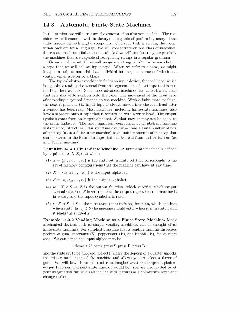
14.3. AUTOMATA, FINITE-STATE MACHINES 127
14.3 Automata, Finite-State MachinesIn this section, we will introduce the concept of an abstract machine. The ma-chines we will examine will (in theory) be capable of performing many of thetasks associated with digital computers. One such task is solving the recog-nition problem for a language. We will concentrate on one class of machines,finite-state machines (finite automata). And we will see that they are preciselythe machines that are capable of recognizing strings in a regular grammar.
Given an alphabet X, we will imagine a string in X∗. to be encoded ona tape that we will call an input tape. When we refer to a tape, we mightimagine a strip of material that is divided into segments, each of which cancontain either a letter or a blank.
The typical abstract machine includes an input device, the read head, whichis capable of reading the symbol from the segment of the input tape that is cur-rently in the read head. Some more advanced machines have a read/write headthat can also write symbols onto the tape. The movement of the input tapeafter reading a symbol depends on the machine. With a finite-state machine,the next segment of the input tape is always moved into the read head aftera symbol has been read. Most machines (including finite-state machines) alsohave a separate output tape that is written on with a write head. The outputsymbols come from an output alphabet, Z, that may or may not be equal tothe input alphabet. The most significant component of an abstract machineis its memory structure. This structure can range from a finite number of bitsof memory (as in a finite-state machine) to an infinite amount of memory thatcan be stored in the form of a tape that can be read from and written on (asin a Turing machine).
Definition 14.3.1 Finite-State Machine. A finite-state machine is definedby a quintet (S,X,Z,w, t) where
(1) S = {s1, s2, . . . , sr} is the state set, a finite set that corresponds to theset of memory configurations that the machine can have at any time.
(2) X = {x1, x2, . . . , xm} is the input alphabet.
(3) Z = {z1, z2, . . . , zn} is the output alphabet.
(4) w : X × S → Z is the output function, which specifies which outputsymbol w(x, s) ∈ Z is written onto the output tape when the machine isin state s and the input symbol x is read.
(5) t : X × S → S is the next-state (or transition) function, which specifieswhich state t(x, s) ∈ S the machine should enter when it is in state s andit reads the symbol x.
Example 14.3.2 Vending Machine as a Finite-State Machine. Manymechanical devices, such as simple vending machines, can be thought of asfinite-state machines. For simplicity, assume that a vending machine dispensespackets of gum, spearmint (S), peppermint (P), and bubble (B), for 25 centseach. We can define the input alphabet to be
{deposit 25 cents,press S,press P, press B}
and the state set to be {Locked, Select}, where the deposit of a quarter unlocksthe release mechanism of the machine and allows you to select a flavor ofgum. We will leave it to the reader to imagine what the output alphabet,output function, and next-state function would be. You are also invited to letyour imagination run wild and include such features as a coin-return lever andchange maker.
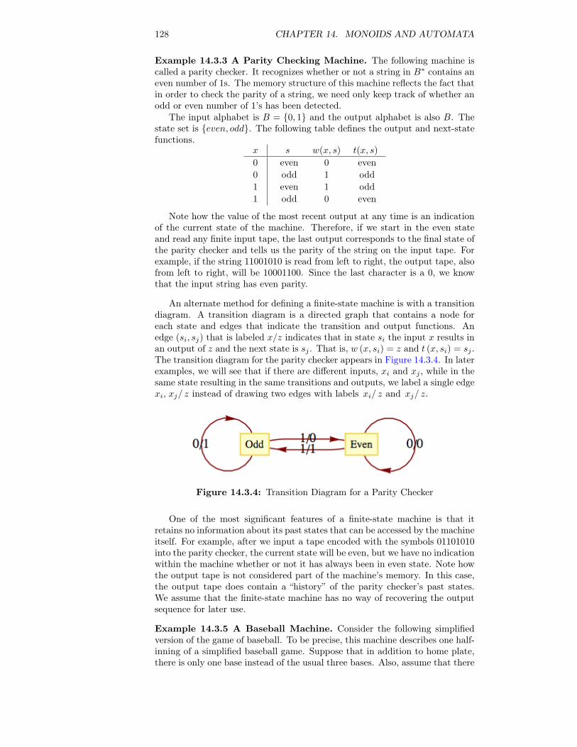
128 CHAPTER 14. MONOIDS AND AUTOMATA
Example 14.3.3 A Parity Checking Machine. The following machine iscalled a parity checker. It recognizes whether or not a string in B∗ contains aneven number of 1s. The memory structure of this machine reflects the fact thatin order to check the parity of a string, we need only keep track of whether anodd or even number of 1’s has been detected.
The input alphabet is B = {0, 1} and the output alphabet is also B. Thestate set is {even, odd}. The following table defines the output and next-statefunctions.
x s w(x, s) t(x, s)
0
0
1
1
evenoddevenodd
0
1
1
0
evenoddoddeven
Note how the value of the most recent output at any time is an indicationof the current state of the machine. Therefore, if we start in the even stateand read any finite input tape, the last output corresponds to the final state ofthe parity checker and tells us the parity of the string on the input tape. Forexample, if the string 11001010 is read from left to right, the output tape, alsofrom left to right, will be 10001100. Since the last character is a 0, we knowthat the input string has even parity.
An alternate method for defining a finite-state machine is with a transitiondiagram. A transition diagram is a directed graph that contains a node foreach state and edges that indicate the transition and output functions. Anedge (si, sj) that is labeled x/z indicates that in state si the input x results inan output of z and the next state is sj . That is, w (x, si) = z and t (x, si) = sj .The transition diagram for the parity checker appears in Figure 14.3.4. In laterexamples, we will see that if there are different inputs, xi and xj , while in thesame state resulting in the same transitions and outputs, we label a single edgexi, xj/ z instead of drawing two edges with labels xi/ z and xj/ z.
Figure 14.3.4: Transition Diagram for a Parity Checker
One of the most significant features of a finite-state machine is that itretains no information about its past states that can be accessed by the machineitself. For example, after we input a tape encoded with the symbols 01101010into the parity checker, the current state will be even, but we have no indicationwithin the machine whether or not it has always been in even state. Note howthe output tape is not considered part of the machine’s memory. In this case,the output tape does contain a “history” of the parity checker’s past states.We assume that the finite-state machine has no way of recovering the outputsequence for later use.
Example 14.3.5 A Baseball Machine. Consider the following simplifiedversion of the game of baseball. To be precise, this machine describes one half-inning of a simplified baseball game. Suppose that in addition to home plate,there is only one base instead of the usual three bases. Also, assume that there
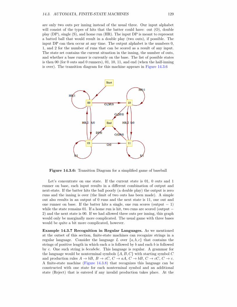
14.3. AUTOMATA, FINITE-STATE MACHINES 129
are only two outs per inning instead of the usual three. Our input alphabetwill consist of the types of hits that the batter could have: out (O), doubleplay (DP), single (S), and home run (HR). The input DP is meant to representa batted ball that would result in a double play (two outs), if possible. Theinput DP can then occur at any time. The output alphabet is the numbers 0,1, and 2 for the number of runs that can be scored as a result of any input.The state set contains the current situation in the inning, the number of outs,and whether a base runner is currently on the base. The list of possible statesis then 00 (for 0 outs and 0 runners), 01, 10, 11, and end (when the half-inningis over). The transition diagram for this machine appears in Figure 14.3.6
Figure 14.3.6: Transition Diagram for a simplified game of baseball
Let’s concentrate on one state. If the current state is 01, 0 outs and 1runner on base, each input results in a different combination of output andnext-state. If the batter hits the ball poorly (a double play) the output is zeroruns and the inning is over (the limit of two outs has been made). A simpleout also results in an output of 0 runs and the next state is 11, one out andone runner on base. If the batter hits a single, one run scores (output = 1)while the state remains 01. If a home run is hit, two runs are scored (output =2) and the next state is 00. If we had allowed three outs per inning, this graphwould only be marginally more complicated. The usual game with three baseswould be quite a bit more complicated, however.
Example 14.3.7 Recognition in Regular Languages. As we mentionedat the outset of this section, finite-state machines can recognize strings in aregular language. Consider the language L over {a, b, c} that contains thestrings of positive length in which each a is followed by b and each b is followedby c. One such string is bccabcbc. This language is regular. A grammar forthe language would be nonterminal symbols {A,B,C} with starting symbol Cand production rules A → bB, B → cC, C → aA, C → bB, C → cC, C → c.A finite-state machine (Figure 14.3.8) that recognizes this language can beconstructed with one state for each nonterminal symbol and an additionalstate (Reject) that is entered if any invalid production takes place. At the
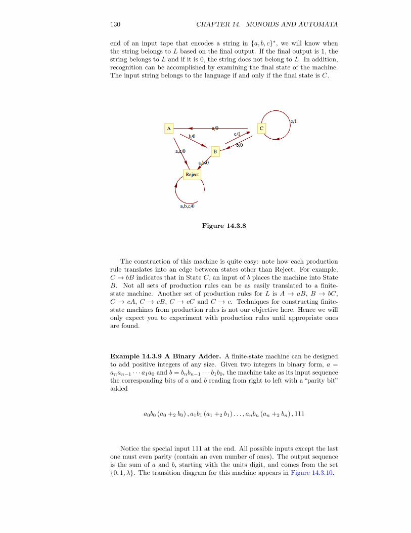
130 CHAPTER 14. MONOIDS AND AUTOMATA
end of an input tape that encodes a string in {a, b, c}∗, we will know whenthe string belongs to L based on the final output. If the final output is 1, thestring belongs to L and if it is 0, the string does not belong to L. In addition,recognition can be accomplished by examining the final state of the machine.The input string belongs to the language if and only if the final state is C.
Figure 14.3.8
The construction of this machine is quite easy: note how each productionrule translates into an edge between states other than Reject. For example,C → bB indicates that in State C, an input of b places the machine into StateB. Not all sets of production rules can be as easily translated to a finite-state machine. Another set of production rules for L is A → aB, B → bC,C → cA, C → cB, C → cC and C → c. Techniques for constructing finite-state machines from production rules is not our objective here. Hence we willonly expect you to experiment with production rules until appropriate onesare found.
Example 14.3.9 A Binary Adder. A finite-state machine can be designedto add positive integers of any size. Given two integers in binary form, a =anan−1 · · · a1a0 and b = bnbn−1 · · · b1b0, the machine take as its input sequencethe corresponding bits of a and b reading from right to left with a “parity bit”added
a0b0 (a0 +2 b0) , a1b1 (a1 +2 b1) . . . , anbn (an +2 bn) , 111
Notice the special input 111 at the end. All possible inputs except the lastone must even parity (contain an even number of ones). The output sequenceis the sum of a and b, starting with the units digit, and comes from the set{0, 1, λ}. The transition diagram for this machine appears in Figure 14.3.10.
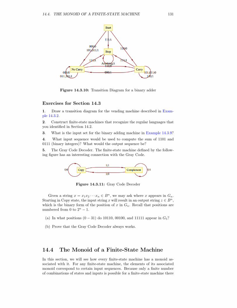
14.4. THE MONOID OF A FINITE-STATE MACHINE 131
Figure 14.3.10: Transition Diagram for a binary adder
Exercises for Section 14.3
1. Draw a transition diagram for the vending machine described in Exam-ple 14.3.2.
2. Construct finite-state machines that recognize the regular languages thatyou identified in Section 14.2.
3. What is the input set for the binary adding machine in Example 14.3.9?
4. What input sequence would be used to compute the sum of 1101 and0111 (binary integers)? What would the output sequence be?
5. The Gray Code Decoder. The finite-state machine defined by the follow-ing figure has an interesting connection with the Gray Code.
Figure 14.3.11: Gray Code Decoder
Given a string x = x1x2 · · ·xn ∈ Bn, we may ask where x appears in Gn.Starting in Copy state, the input string x will result in an output string z ∈ Bn,which is the binary form of the position of x in Gn. Recall that positions arenumbered from 0 to 2n − 1.
(a) In what positions (0− 31) do 10110, 00100, and 11111 appear in G5?
(b) Prove that the Gray Code Decoder always works.
14.4 The Monoid of a Finite-State Machine
In this section, we will see how every finite-state machine has a monoid as-sociated with it. For any finite-state machine, the elements of its associatedmonoid correspond to certain input sequences. Because only a finite numberof combinations of states and inputs is possible for a finite-state machine there
132 CHAPTER 14. MONOIDS AND AUTOMATA
is only a finite number of input sequences that summarize the machine. Thisidea is illustrated best with a few examples.
Consider the parity checker. The following table summarizes the effect onthe parity checker of strings in B1 and B2. The row labeled “Even” containsthe final state and final output as a result of each input string in B1 and B2
when the machine starts in the even state. Similarly, the row labeled “Odd”contains the same information for input sequences when the machine starts inthe odd state.
Input String 0 1 00 01 10 11
Even ( Even, 0) ( Odd, 1) ( Even, 0) ( Odd, 1) ( Odd, 1) ( Even, 0)
Odd ( Odd, 1) ( Even, 1) ( Odd, 1) ( Even, 1) ( Even, 0) ( Odd, 1)
Same Effect as 0 1 1 0
Note how, as indicated in the last row, the strings in B2 have the sameeffect as certain strings in B1. For this reason, we can summarize the machinein terms of how it is affected by strings of length 1. The actual monoid thatwe will now describe consists of a set of functions, and the operation on thefunctions will be based on the concatenation operation.
Let T0 be the final effect (state and output) on the parity checker of theinput 0. Similarly, T1 is defined as the final effect on the parity checker of theinput 1. More precisely,
T0( even) = ( even, 0) and T0( odd) = ( odd, 1),
whileT1( even) = ( odd, 1) and T1( odd) = ( even, 0).
In general, we define the operation on a set of such functions as follows: if s,t are input sequences and Ts and Tt, are functions as above, then Ts ∗Tt = Tst,that is, the result of the function that summarizes the effect on the machine bythe concatenation of s with t. Since, for example, 01 has the same effect on theparity checker as 1, T0 ∗ T1 = T01 = T1. We don’t stop our calculation at T01
because we want to use the shortest string of inputs to describe the final result.
A complete table for the monoid of the parity checker is∗ T0 T1
T0
T1
T0 T1
T1 T0
What is the identity of this monoid? The monoid of the parity checker isisomorphic to the monoid [Z2; +2].
This operation may remind you of the composition operation on functions,but there are two principal differences. The domain of Ts is not the codomainof Tt and the functions are read from left to right unlike in composition, wherethey are normally read from right to left.
You may have noticed that the output of the parity checker echoes the stateof the machine and that we could have looked only at the effect on the machineas the final state. The following example has the same property, hence we willonly consider the final state.
Example 14.4.1. The transition diagram for the machine that recognizesstrings in B∗ that have no consecutive 1’s appears in Figure 14.4.2. Note howit is similar to the graph in Figure 9.0.1. Only a “reject state” has been added,for the case when an input of 1 occurs while in State a. We construct a similartable to the one in the previous example to study the effect of certain stringson this machine. This time, we must include strings of length 3 before werecognize that no “new effects” can be found.
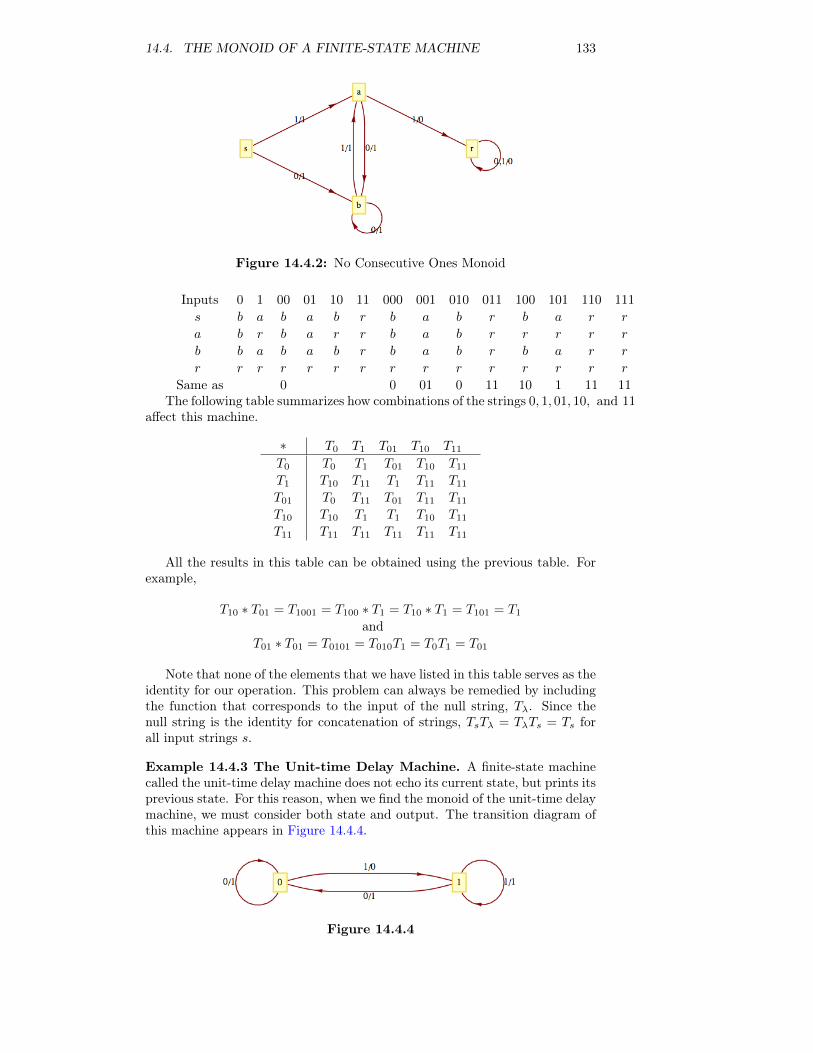
14.4. THE MONOID OF A FINITE-STATE MACHINE 133
Figure 14.4.2: No Consecutive Ones Monoid
Inputs 0 1 00 01 10 11 000 001 010 011 100 101 110 111
s b a b a b r b a b r b a r r
a b r b a r r b a b r r r r r
b b a b a b r b a b r b a r r
r r r r r r r r r r r r r r r
Same as 0 0 01 0 11 10 1 11 11The following table summarizes how combinations of the strings 0, 1, 01, 10, and 11
affect this machine.
∗ T0 T1 T01 T10 T11
T0
T1
T01
T10
T11
T0 T1 T01 T10 T11
T10 T11 T1 T11 T11
T0 T11 T01 T11 T11
T10 T1 T1 T10 T11
T11 T11 T11 T11 T11
All the results in this table can be obtained using the previous table. Forexample,
T10 ∗ T01 = T1001 = T100 ∗ T1 = T10 ∗ T1 = T101 = T1
andT01 ∗ T01 = T0101 = T010T1 = T0T1 = T01
Note that none of the elements that we have listed in this table serves as theidentity for our operation. This problem can always be remedied by includingthe function that corresponds to the input of the null string, Tλ. Since thenull string is the identity for concatenation of strings, TsTλ = TλTs = Ts forall input strings s.
Example 14.4.3 The Unit-time Delay Machine. A finite-state machinecalled the unit-time delay machine does not echo its current state, but prints itsprevious state. For this reason, when we find the monoid of the unit-time delaymachine, we must consider both state and output. The transition diagram ofthis machine appears in Figure 14.4.4.
Figure 14.4.4
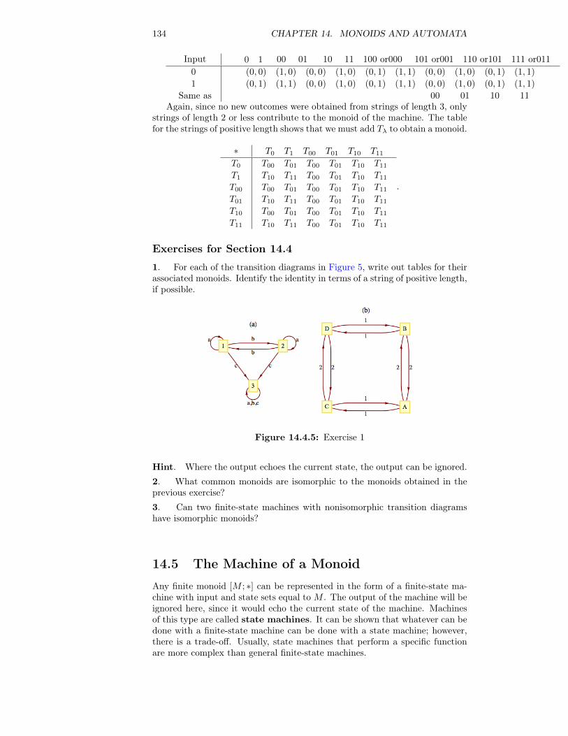
134 CHAPTER 14. MONOIDS AND AUTOMATA
Input 0 1 00 01 10 11 100 or000 101 or001 110 or101 111 or011
0
1
Same as
(0, 0) (1, 0) (0, 0) (1, 0) (0, 1) (1, 1) (0, 0) (1, 0) (0, 1) (1, 1)
(0, 1) (1, 1) (0, 0) (1, 0) (0, 1) (1, 1) (0, 0) (1, 0) (0, 1) (1, 1)
00 01 10 11Again, since no new outcomes were obtained from strings of length 3, only
strings of length 2 or less contribute to the monoid of the machine. The tablefor the strings of positive length shows that we must add Tλ to obtain a monoid.
∗ T0 T1 T00 T01 T10 T11
T0
T1
T00
T01
T10
T11
T00 T01 T00 T01 T10 T11
T10 T11 T00 T01 T10 T11
T00 T01 T00 T01 T10 T11
T10 T11 T00 T01 T10 T11
T00 T01 T00 T01 T10 T11
T10 T11 T00 T01 T10 T11
.
Exercises for Section 14.4
1. For each of the transition diagrams in Figure 5, write out tables for theirassociated monoids. Identify the identity in terms of a string of positive length,if possible.
Figure 14.4.5: Exercise 1
Hint. Where the output echoes the current state, the output can be ignored.2. What common monoids are isomorphic to the monoids obtained in theprevious exercise?3. Can two finite-state machines with nonisomorphic transition diagramshave isomorphic monoids?
14.5 The Machine of a Monoid
Any finite monoid [M ; ∗] can be represented in the form of a finite-state ma-chine with input and state sets equal to M . The output of the machine will beignored here, since it would echo the current state of the machine. Machinesof this type are called state machines. It can be shown that whatever can bedone with a finite-state machine can be done with a state machine; however,there is a trade-off. Usually, state machines that perform a specific functionare more complex than general finite-state machines.
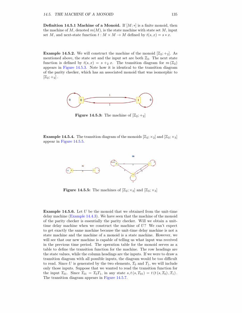
14.5. THE MACHINE OF A MONOID 135
Definition 14.5.1 Machine of a Monoid. If [M ; ∗] is a finite monoid, thenthe machine ofM , denotedm(M), is the state machine with state setM , inputset M , and next-state function t : M ×M →M defined by t(s, x) = s ∗ x.
Example 14.5.2. We will construct the machine of the monoid [Z2; +2]. Asmentioned above, the state set and the input set are both Z2. The next statefunction is defined by t(s, x) = s +2 x. The transition diagram for m (Z2)appears in Figure 14.5.3. Note how it is identical to the transition diagramof the parity checker, which has an associated monoid that was isomorphic to[Z2; +2] .
Figure 14.5.3: The machine of [Z2; +2]
Example 14.5.4. The transition diagram of the monoids [Z2;×2] and [Z3;×3]appear in Figure 14.5.5.
Figure 14.5.5: The machines of [Z2;×2] and [Z3;×3]
Example 14.5.6. Let U be the monoid that we obtained from the unit-timedelay machine (Example 14.4.3). We have seen that the machine of the monoidof the parity checker is essentially the parity checker. Will we obtain a unit-time delay machine when we construct the machine of U? We can’t expectto get exactly the same machine because the unit-time delay machine is not astate machine and the machine of a monoid is a state machine. However, wewill see that our new machine is capable of telling us what input was receivedin the previous time period. The operation table for the monoid serves as atable to define the transition function for the machine. The row headings arethe state values, while the column headings are the inputs. If we were to draw atransition diagram with all possible inputs, the diagram would be too difficultto read. Since U is generated by the two elements, T0 and T1, we will includeonly those inputs. Suppose that we wanted to read the transition function forthe input T01. Since T01 = T0T1, in any state s, t (s, T01) = t (t (s, T0) , T1) .The transition diagram appears in Figure 14.5.7.
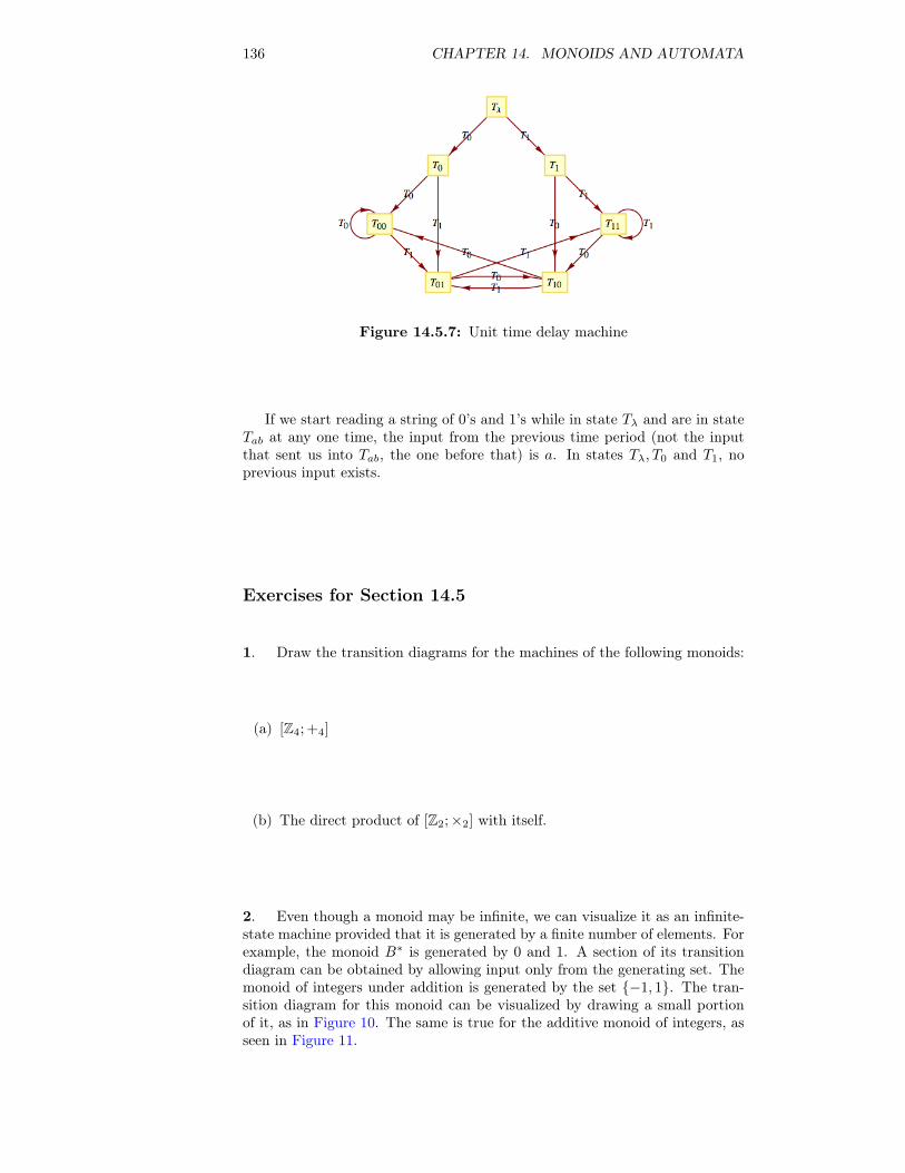
136 CHAPTER 14. MONOIDS AND AUTOMATA
Figure 14.5.7: Unit time delay machine
If we start reading a string of 0’s and 1’s while in state Tλ and are in stateTab at any one time, the input from the previous time period (not the inputthat sent us into Tab, the one before that) is a. In states Tλ, T0 and T1, noprevious input exists.
Exercises for Section 14.5
1. Draw the transition diagrams for the machines of the following monoids:
(a) [Z4; +4]
(b) The direct product of [Z2;×2] with itself.
2. Even though a monoid may be infinite, we can visualize it as an infinite-state machine provided that it is generated by a finite number of elements. Forexample, the monoid B∗ is generated by 0 and 1. A section of its transitiondiagram can be obtained by allowing input only from the generating set. Themonoid of integers under addition is generated by the set {−1, 1}. The tran-sition diagram for this monoid can be visualized by drawing a small portionof it, as in Figure 10. The same is true for the additive monoid of integers, asseen in Figure 11.
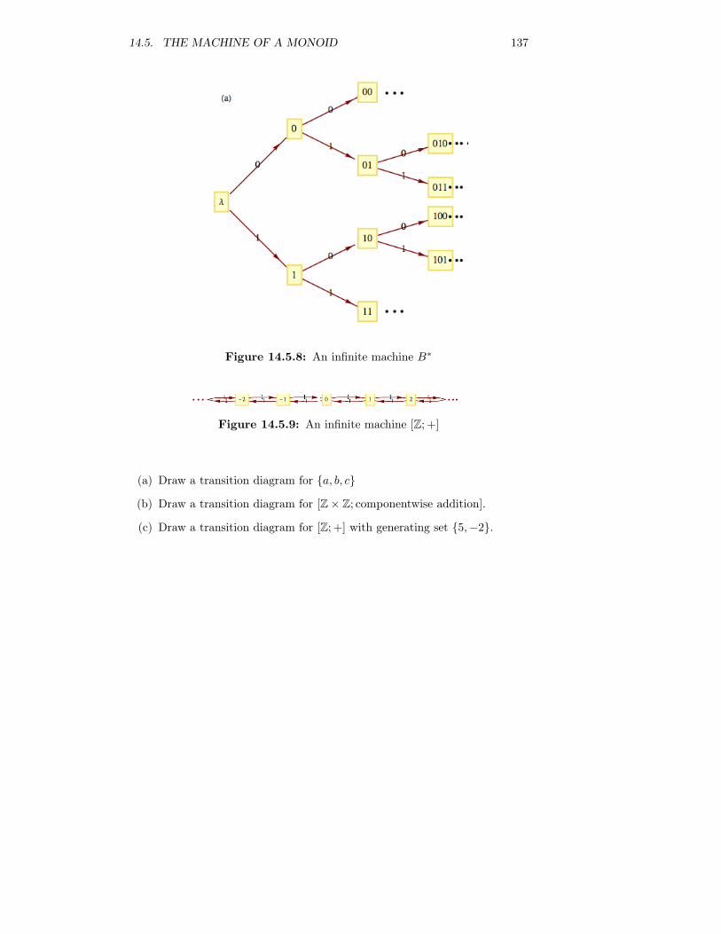
14.5. THE MACHINE OF A MONOID 137
Figure 14.5.8: An infinite machine B∗
Figure 14.5.9: An infinite machine [Z; +]
(a) Draw a transition diagram for {a, b, c}
(b) Draw a transition diagram for [Z× Z; componentwise addition].
(c) Draw a transition diagram for [Z; +] with generating set {5,−2}.

138 CHAPTER 14. MONOIDS AND AUTOMATA
Chapter 15
Group Theory andApplications
Abelian Group
In Abelian groups, when computing,With operands there’s no refuting:The expression bcIs the same as cb.Not en route to your job, yet commuting.
Howard Spindel, The Omnificent English Dictionary In Limerick Form
In Chapter 11, we introduced groups as a typical algebraic system. The associ-ated concepts of subgroup, group isomorphism, and direct products of groupswere also introduced. Groups were chosen for that chapter because they areamong the simplest types of algebraic systems. Despite this simplicity, grouptheory abounds with interesting applications. In this chapter we will introducesome more important concepts in elementary group theory, and some of theirapplications.
15.1 Cyclic GroupsGroups are classified according to their size and structure. A group’s structureis revealed by a study of its subgroups and other properties (e.g., whether itis abelian) that might give an overview of it. Cyclic groups have the simpleststructure of all groups.
Definition 15.1.1 Cyclic Group. Group G is cyclic if there exists a ∈ Gsuch that the cyclic subgroup generated by a, 〈a〉, equals all of G. That is,G = {na|n ∈ Z}, in which case a is called a generator of G. The reader shouldnote that additive notation is used for G.
Example 15.1.2 A Finite Cyclic Group. Z12 = [Z12; +12], where +12 isaddition modulo 12, is a cyclic group. To verify this statement, all we need todo is demonstrate that some element of Z12 is a generator. One such elementis 5; that is, 〈5〉 = Z12. One more obvious generator is 1. In fact, 1 is agenerator of every [Zn; +n]. The reader is asked to prove that if an element isa generator, then its inverse is also a generator. Thus, −5 = 7 and −1 = 11are the other generators of Z12. The remaining eight elements of the group arenot generators.
139
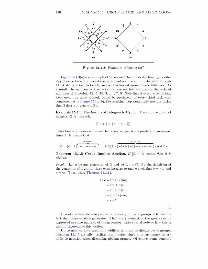
140 CHAPTER 15. GROUP THEORY AND APPLICATIONS
Figure 15.1.3: Examples of “string art”
Figure 15.1.3(a) is an example of “string art” that illustrates how 5 generatesZ12. Twelve tacks are placed evenly around a circle and numbered 0 through11. A string is tied to tack 0, and is then looped around every fifth tack. Asa result, the numbers of the tacks that are reached are exactly the orderedmultiples of 5 modulo 12: 5, 10, 3, ... , 7, 0. Note that if every seventh tackwere used, the same artwork would be produced. If every third tack wereconnected, as in Figure 15.1.3(b), the resulting loop would only use four tacks;thus 3 does not generate Z12.
Example 15.1.4 The Group of Integers is Cyclic. The additive group ofintegers, [Z; +], is cyclic:
Z = 〈1〉 = {n · 1|n ∈ Z}
This observation does not mean that every integer is the product of an integertimes 1. It means that
Z = {0} ∪ {n terms︷ ︸︸ ︷
1 + 1 + · · ·+ 1 | n ∈ P} ∪ {n terms︷ ︸︸ ︷
(−1) + (−1) + · · ·+ (−1) | n ∈ P}
Theorem 15.1.5 Cyclic Implies Abelian. If [G; ∗] is cyclic, then it isabelian.
Proof. Let a be any generator of G and let b, c ∈ G. By the definition ofthe generator of a group, there exist integers m and n such that b = ma andc = na. Thus, using Theorem 11.3.14,
b ∗ c = (ma) ∗ (na)
= (m+ n)a
= (n+m)a
= (na) ∗ (ma)
= c ∗ b
One of the first steps in proving a property of cyclic groups is to use thefact that there exists a generator. Then every element of the group can beexpressed as some multiple of the generator. Take special note of how this isused in theorems of this section.
Up to now we have used only additive notation to discuss cyclic groups.Theorem 15.1.5 actually justifies this practice since it is customary to useadditive notation when discussing abelian groups. Of course, some concrete
15.1. CYCLIC GROUPS 141
groups for which we employ multiplicative notation are cyclic. If one of itselements, a, is a generator,
〈a〉 = {an | n ∈ Z}
Example 15.1.6 A Cyclic Multiplicative Group. The group of positiveintegers modulo 11 with modulo 11 multiplication, [Z∗11;×11], is cyclic. Oneof its generators is 6: 61 = 6, 62 = 3, 63 = 7,. . . , 69 = 2, and 610 = 1, theidentity of the group.
Example 15.1.7 A Non-cyclic Group. The real numbers with addition,[R; +] is a noncyclic group. The proof of this statement requires a bit moregenerality since we are saying that for all r ∈ R, 〈r〉 is a proper subset ofR. If r is nonzero, the multiples of r are distributed over the real line, as inFigure 15.1.8. It is clear then that there are many real numbers, like r/2, thatare not in 〈r〉.
Figure 15.1.8: Elements of 〈r〉, r > 0
The next two proofs make use of the Theorem 11.4.1.The following theorem shows that a cyclic group can never be very compli-
cated.
Theorem 15.1.9 Possible Cyclic Group Structures. If G is a cyclicgroup, then G is either finite or countably infinite. If G is finite and |G| = n,it is isomorphic to [Zn; +n]. If G is infinite, it is isomorphic to [Z; +].
Proof. Case 1: |G| < ∞. If a is a generator of G and |G| = n, defineφ : Zn → G by φ(k) = ka for all k ∈ Zn.
Since 〈a〉 is finite, we can use the fact that the elements of 〈a〉 are thefirst n nonnegative multiples of a. From this observation, we see that φ is asurjection. A surjection between finite sets of the same cardinality must be abijection. Finally, if p, q ∈ Zn,
φ(p) + φ(q) = pa+ qa
= (p+ q)a
= (p+n q)a see exercise 10= φ(p+n q)
Therefore φ is an isomorphism.Case 2: |G| =∞. We will leave this case as an exercise.
Theorem 15.1.10 Subgroups of Cyclic Groups. Every subgroup of acyclic group is cyclic.
Proof. Let G be cyclic with generator a and let H ≤ G. If H = {e}, Hhas e as a generator. We may now assume that |H| ≥ 2 and a 6= e. Letm be the least positive integer such that ma belongs to H. This is the keystep. It lets us get our hands on a generator of H. We will now show thatc = ma generates H. Certainly, 〈c〉 ⊆ H, but suppose that 〈c〉 6= H. Thenthere exists b ∈ H such that b /∈ 〈c〉. Now, since b is in G, there exists n ∈ Zsuch that b = na. We now apply the division property and divide n by m.b = na = (qm + r)a = (qm)a + ra, where 0 ≤ r < m. We note that r cannotbe zero for otherwise we would have b = na = q(ma) = qc ∈ 〈c〉. Therefore,ra = na−(qm)a ∈ H. This contradicts our choice ofm because 0 < r < m.
142 CHAPTER 15. GROUP THEORY AND APPLICATIONS
Example 15.1.11 All subgroups of Z10. The only proper subgroups of Z10
are H1 = {0, 5} and H2 = {0, 2, 4, 6, 8}. They are both cyclic: H1 = 〈5〉, whileH2 = 〈2〉 = 〈4〉 = 〈6〉 = 〈8〉. The generators of Z10 are 1, 3, 7, and 9.
Example 15.1.12 All subgroups of Z. With the exception of {0}, all sub-groups of Z are isomorphic to Z. If H ≤ Z, then H is the cyclic subgroupgenerated by the least positive element of H. It is infinite and so by Theo-rem 15.1.10 it is isomorphic to Z.
We now cite a useful theorem for computing the order of cyclic subgroupsof a cyclic group:
Theorem 15.1.13 The order of elements of a finite cyclic group. If Gis a cyclic group of order n and a is a generator of G, the order of ka is n/d,where d is the greatest common divisor of n and k.
Proof. The proof of this theorem is left to the reader.
Example 15.1.14 Computation of an order in a cyclic group. To com-pute the order of 〈18〉 in Z30, we first observe that 1 is a generator of Z30 and18 = 18(1). The greatest common divisor of 18 and 30 is 6. Hence, the orderof 〈18〉 is 30/6, or 5.
At this point, we will introduce the idea of a fast adder, a relatively modernapplication (Winograd, 1965) of an ancient theorem, the Chinese RemainderTheorem. We will present only an overview of the theory and rely primarilyon examples.
Out of necessity, integer addition with a computer is addition modulo n,for n some larger number. Consider the case where n is small, like 64. Thenaddition involves the addition of six-digit binary numbers. Consider the processof adding 31 and 1. Assume the computer’s adder takes as input two bitstrings a = {a0, a1, a2, a3, a4, a5} and b = {b0, b1, b2, b3, b4, b5} and outputss = {s0, s1, s2, s3, s4, s5}, the sum of a and b. Then, if a = 31 = (1, 1, 1, 1, 1, 0)and b = 1 = (1, 0, 0, 0, 0, 0), s will be (0, 0, 0, 0, 0, 1), or 32. The outputs = 1 cannot be determined until all other outputs have been determined. Ifaddition is done with a finite-state machine, as in Example 14.3.9, the timerequired to get s will be six time units, where one time unit is the time it takesto get one output from the machine. In general, the time required to obtains will be proportional to the number of bits. Theoretically, this time can bedecreased, but the explanation would require a long digression and our relativeresults would not change that much. We will use the rule that the number oftime units needed to perform addition modulo n is proportional to dlog2 ne.
Now we will introduce a hypothetical problem that we will use to illustratethe idea of a fast adder. Suppose that we had to add 1,000 numbers modulo27720 = 8 · 9 · 5 · 7 · 11. By the rule above, since 214 < 27720 < 215, eachaddition would take 15 time units. If the sum is initialized to zero, 1,000additions would be needed; thus, 15,000 time units would be needed to do theadditions. We can improve this time dramatically by applying the ChineseRemainder Theorem.
Theorem 15.1.15 Chinese Remainder Theorem (CRT). Let n1, n2, . . .,np be integers that have no common factor greater than one between any pairof them; i. e., they are relatively prime. Let n = n1n2 · · ·np. Define
θ : Zn → Zn1× Zn2
× · · · × Znp
byθ(k) = (k1, k2, . . . , kp)
15.1. CYCLIC GROUPS 143
where for 1 ≤ i ≤ p, 0 ≤ ki < ni and k ≡ ki (mod ni). Then θ is anisomorphism from Zn into Zn1 × Zn2 × · · · × Znp .
The Chinese Remainder Theorem can be stated in several different forms,and its proof can be found in many abstract algebra texts.
As we saw in Chapter 11, Z6 is isomorphic to Z2×Z3 . This is the smallestcase to which the CRT can be applied. An isomorphism between Z6 and Z2×Z3
isθ(0) = (0, 0) θ(3) = (1, 0)
θ(1) = (1, 1) θ(4) = (0, 1)
θ(2) = (0, 2) θ(5) = (1, 2)
Let’s consider a somewhat larger case. We start by selecting a modulusthat can be factored into a product of relatively prime integers: n = 21, 600 =253352. In this case the factors are 25 = 32, 33 = 27, and 52 = 25. Theyneed not be powers of primes, but it is easy to break the factors into thisform to assure relatively prime numbers. To add in Zn, we need dlog2 ne = 15time units. Let G = Z32 × Z27 × Z25. The CRT gives us an isomorphismbetween Z21600 and G. The basic idea behind the fast adder, illustrated inFigure 15.1.16, is to make use of this isomorphism. The notation x += a isinterpreted as the instruction to add the value of a to the variable x.
Figure 15.1.16: Fast Adder Scheme
Assume we have several integers a1, . . . , am to be added. Here, we assumem = 20. We compute the sum s to compare our result with this true sum.
a=[1878 ,1384 ,84 ,2021 ,784 ,1509 ,1740 ,1201 ,2363 ,1774 ,1865 ,33 ,1477 ,894 ,690 ,520 ,198 ,1349 ,1278 ,650]
s =0for t in a:
s+=ts
23692
Although out sum is an integer calculation, we will put our calculation inthe context of the integers modulo 21600. The isomophism from Z21600 intoG = Z32 × Z27 × Z25 is defined in Sage as theta. In addition we demonstratethat the operations in these groups are preserved by theta.
G=cartesian_product ([ Integers (32),Integers (27),Integers (25)])def theta(x):
return G((x%32,x%27,x%25))[theta (1878)+theta (1384) ,theta (1878+1384)]
[(30, 22, 12), (30, 22, 12)]
144 CHAPTER 15. GROUP THEORY AND APPLICATIONS
We initialize the sums in each factor of the range of theta to zero and decom-pose each summand t into a triple θ(t) = (t1, t2, t3) ∈ G.
sum=G((0,0,0))for t in a:
sum+=theta(t)sum
(12, 13, 17)
Addition in G can be done in parallel so that each new subtotal in the formof the triple (s1, s2, s3) takes only as long to compute as it takes to add in thelargest modulus, log2 32 = 5 time units, if calculations are done in parallel.By the time rule that we have established, the addition of 20 numbers can bedone in 20 · 5 = 100 time units, as opposed to 20 · 15 = 300 time units if we dothe calculations in Z21600. However the result is a triple in G. The functionthat performs the inverse of theta is built into most mathematics programs,including Sage. In Sage the function is crt. We use this function to computethe inverse of our triple, which is an element of Z21600. The result isn’t thetrue sum because the the modulus 21600 is not large enough. However, weverify that our result is congruent to the true sum modulo 21600.
isum=crt ([12 ,13 ,17] ,[32 ,27 ,25])[isum ,(s-isum)%(21600)]
[2092, 0]
In order to get the true sum from our scheme, the modulus would need to beincreased by moving from 21600 to, for example, 21600∗23 = 496800. Mappinginto the new group, G = Z32×Z27×Z25×Z23 will take slightly longer, as willthe inversion process with crt, but adding the summands that are in the formof quadruples can be done with no additional time.
The computation of θ−1 (s1, s2, s3) that is done by the Sage function crtcan be accomplished in a variety of ways. All of them ultimately are sim-plified by the fact that θ−1 is also an isomorphism. One approach is touse the isomorphism property to realize that the value of θ−1 (s1, s2, s3) iss1θ−1(1, 0, 0)+s2θ
−1(0, 1, 0)+s3θ−1(0, 0, 1). The arithmetic in this expression
is in the domain of θ and is more time consuming, but it need only be doneonce. This is why the fast adder is only practical in situations where manyadditions must be performed to get a single sum.
The inverse images of the “unit vectors” can be computed ahead of time.
u=[crt ([1 ,0 ,0] ,[32 ,27 ,25]),crt ([0 ,1 ,0] ,[32 ,27 ,25]),crt ([0 ,0 ,1] ,[32 ,27 ,25])]
u
[7425, 6400, 7776]
The result we computed earlier can be computed directly by in the largermodulus.
(7425*12 + 6400*13+ 7776* 17) %21600
2092
To further illustrate the potential of fast adders, consider increasing the mod-ulus to n = 2533527211 · 13 · 17 · 19 · 23 · 29 · 31 · 37 · 41 · 43 · 47 ≈ 3.1 × 10²¹.Each addition using the usual modulo n addition with full adders would take72 time units. By decomposing each summand into 15-tuples according to theCRT, the time is reduced to dlog2 49e = 6 time units per addition.
15.2. COSETS AND FACTOR GROUPS 145
Exercises for Section 15.1
1. What generators besides 1 does [Z; +] have?2. Without doing any multiplications, determine the number of generatorsof [Z11; +11].3. Prove that if |G| > 2 and G is cyclic, G has at least two generators.4. If you wanted to list the generators of Zn you would only have to test thefirst n/2 positive integers. Why?5. Which of the following groups are cyclic? Explain.
(a) [Q; +]
(b) [R+; ·]
(c) [6Z; +] where 6Z = {6n|n ∈ Z}
(d) Z× Z
(e) Z2 × Z3 × Z25
6. For each group and element, determine the order of the cyclic subgroupgenerated by the element:
(a) Z25 , 15
(b) Z4 × Z9 , (2, 6) (apply Exercise 8)
(c) Z64 , 2
7. How can Theorem 15.1.13 be applied to list the generators of Zn? Whatare the generators of Z25? Of Z256?8. Prove that if the greatest common divisor of n and m is 1, then (1, 1) isa generator of Zn × Zm, and hence, Zn × Zm is isomorphic to Znm.9.
(a) Illustrate how the fast adder can be used to add the numbers 21, 5, 7,and 15 using the isomorphism between Z77 and Z7 × Z11.
(b) If the same isomorphism is used to add the numbers 25, 26, and 40, whatwould the result be, why would it be incorrect, and how would the answerdiffer from the answer in part a?
10. Prove that if G. is a cyclic group of order n . with generator a, andp, q ∈ {0, 1, . . . , n− 1}, then (p+ q)a = (p+n q) a
15.2 Cosets and Factor Groups
Consider the group [Z12; +12]. As we saw in the previous section, we canpicture its cyclic properties with the string art of Figure 15.1.3. Here we willbe interested in the non-generators, like 3. The solid lines in Figure 15.2.1show that only one-third of the tacks have been reached by starting at zeroand jumping to every third tack. The numbers of these tacks correspond to〈3〉 = {0, 3, 6, 9}.
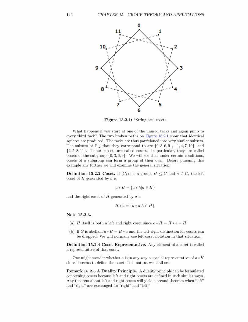
146 CHAPTER 15. GROUP THEORY AND APPLICATIONS
Figure 15.2.1: “String art” cosets
What happens if you start at one of the unused tacks and again jump toevery third tack? The two broken paths on Figure 15.2.1 show that identicalsquares are produced. The tacks are thus partitioned into very similar subsets.The subsets of Z12 that they correspond to are {0, 3, 6, 9}, {1, 4, 7, 10}, and{2, 5, 8, 11}. These subsets are called cosets. In particular, they are calledcosets of the subgroup {0, 3, 6, 9}. We will see that under certain conditions,cosets of a subgroup can form a group of their own. Before pursuing thisexample any further we will examine the general situation.
Definition 15.2.2 Coset. If [G; ∗] is a group, H ≤ G and a ∈ G, the leftcoset of H generated by a is
a ∗H = {a ∗ h|h ∈ H}
and the right coset of H generated by a is
H ∗ a = {h ∗ a|h ∈ H}.
Note 15.2.3.
(a) H itself is both a left and right coset since e ∗H = H ∗ e = H.
(b) If G is abelian, a ∗H = H ∗ a and the left-right distinction for cosets canbe dropped. We will normally use left coset notation in that situation.
Definition 15.2.4 Coset Representative. Any element of a coset is calleda representative of that coset.
One might wonder whether a is in any way a special representative of a∗Hsince it seems to define the coset. It is not, as we shall see.
Remark 15.2.5 A Duality Principle. A duality principle can be formulatedconcerning cosets because left and right cosets are defined in such similar ways.Any theorem about left and right cosets will yield a second theorem when “left”and “right” are exchanged for “right” and “left.”
15.2. COSETS AND FACTOR GROUPS 147
Theorem 15.2.6. If b ∈ a ∗ H, then a ∗ H = b ∗ H, and if b ∈ H ∗ a, thenH ∗ a = H ∗ b.
Proof. In light of the remark above, we need only prove the first part of thistheorem. Suppose that x ∈ a ∗H. We need only find a way of expressing x as“b times an element of H.” Then we will have proven that a ∗H ⊆ b ∗H. Bythe definition of a ∗H, since b and x are in a ∗H, there exist h1 and h2 in Hsuch that b = a ∗ h1 and x = a ∗ h2. Given these two equations, a = bh−1
1 and
x = a ∗ h2 = (b ∗ h−11 ) ∗ h2 = b ∗ (h−1
1 ∗ h2)
Since h1, h2 ∈ H, h−11 ∗ h2 ∈ H, and we are done with this part of the proof.
In order to show that b ∗H ⊆ a ∗H, one can follow essentially the same steps,which we will let the reader fill in.
Example 15.2.7. In Figure 15.2.1, you can start at either 1 or 7 and obtainthe same path by taking jumps of three tacks in each step. Thus,
1 +12 {0, 3, 6, 9} = 7 +12 {0, 3, 6, 9} = {1, 4, 7, 10}.
The set of left (or right) cosets of a subgroup partition a group in a specialway:
Theorem 15.2.8 Cosets Partition a Group. If [G; ∗] is a group and H ≤G, the set of left cosets of H is a partition of G. In addition, all of the leftcosets of H have the same cardinality. The same is true for right cosets.
Proof. That every element ofG belongs to a left coset is clear because a ∈ a∗Hfor all a ∈ G. If a∗H and b∗H are left cosets, we will prove that they are eitherequal or disjoint. If a ∗H and b ∗H are not disjoint, a ∗H ∩ b ∗H is nonemptyand some element c ∈ G belongs to the intersection. Then by Theorem 15.2.6,c ∈ a ∗H ⇒ a ∗H = c ∗H and c ∈ b ∗H ⇒ b ∗H = c ∗H. Hence a ∗H = b ∗H.
We complete the proof by showing that each left coset has the same car-dinality as H. To do this, we simply observe that if a ∈ G, ρ : H → a ∗ Hdefined by ρ(h) = a ∗ h is a bijection and hence |H| = |a ∗H|. We will leavethe proof of this statement to the reader.
The function ρ has a nice interpretation in terms of our opening example.If a ∈ Z12, the graph of {0, 3, 6, 9} is rotated (30a)◦ to coincide with one of thethree cosets of {0, 3, 6, 9}.
Corollary 15.2.9 A Coset Counting Formula. If |G| < ∞ and H ≤ G,the number of distinct left cosets of H equals |G||H| . For this reason we use G/Hto denote the set of left cosets of H in G
Proof. This follows from the partitioning of G into equal sized sets, one ofwhich is H.
Example 15.2.10. The set of integer multiples of four, 4Z, is a subgroup of[Z; +]. Four distinct cosets of 4Z partition the integers. They are 4Z, 1 + 4Z,2 + 4Z, and 3 + 4Z, where, for example, 1 + 4Z = {1 + 4k|k ∈ Z}. 4Z can alsobe written 0 + 4Z.
Convention 15.2.11 Distinguished Representatives. Although we haveseen that any representative can describe a coset, it is often convenient toselect a distinguished representative from each coset. The advantage to doingthis is that there is a unique name for each coset in terms of its distinguishedrepresentative. In numeric examples such as the one above, the distinguished
148 CHAPTER 15. GROUP THEORY AND APPLICATIONS
representative is usually the smallest nonnegative representative. Remember,this is purely a convenience and there is absolutely nothing wrong in writing−203+4Z, 5+4Z, or 621+4Z in place of 1+4Z because −203, 5, 621 ∈ 1+4Z.
Before completing the main thrust of this section, we will make note of asignificant implication of Theorem 15.2.8. Since a finite group is divided intocosets of a common size by any subgroup, we can conclude:
Theorem 15.2.12 Lagrange’s Theorem. The order of a subgroup of a finitegroup must divide the order of the group.
One immediate implication of Lagrange’s Theorem is that if p is prime, Zphas no proper subgroups.
We will now describe the operation on cosets which will, under certaincircumstances, result in a group. For most of this section, we will assume thatG is an abelian group. This is one sufficient (but not necessary) condition thatguarantees that the set of left cosets will form a group.
Definition 15.2.13 Operation on Cosets. Let C and D be left cosets ofH, a subgroup of G with representatives c and d, respectively. Then
C ⊗D = (c ∗H)⊗ (d ∗H) = (c ∗ d) ∗H
The operation ⊗ is called the operation induced on left cosets by ∗.
In Theorem 15.2.18, later in this section, we will prove that if G is anabelian group, ⊗ is indeed an operation. In practice, if the group G is anadditive group, the symbol ⊗ is replaced by +, as in the following example.
Example 15.2.14 Computing with cosets of 4Z. Consider the cosets de-scribed in Example 15.2.10. For brevity, we rename 0 + 4Z, 1 + 4Z, 2 + 4Z,and 3 + 4Z with the symbols 0, 1, 2, and 3. Let’s do a typical calculation,1 + 3. We will see that the result is always going to be 0 , no matter whatrepresentatives we select. For example, 9 ∈ 1, 7 ∈ 3, and 9 + 7 = 16 ∈ 0. Ourchoice of the representatives 1 and 3 were completely arbitrary.
In general, C ⊗ D can be computed in many ways, and so it is necessaryto show that the choice of representatives does not affect the result. When theresult we get for C ⊗D is always independent of our choice of representatives,we say that “⊗ is well defined.” Addition of cosets is a well-defined operationon the left cosets of 4Z and is summarized in the following table. Do you noticeanything familiar?
⊗ 0 1 2 3
0 0 1 2 3
1 1 2 3 0
2 2 3 0 1
3 3 0 1 2
Example 15.2.15 Cosets of the integers in the group of Real numbers.Consider the group of real numbers, [R; +], and its subgroup of integers, Z.Every element of R/Z has the same cardinality as Z. Let s, t ∈ R. s ∈ t + Zif s can be written t + n for some n ∈ Z. Hence s and t belong to the samecoset if they differ by an integer. (See Exercise 15.2.6 for a generalization ofthis fact.)
Now consider the coset 0.25+Z. Real numbers that differ by an integer from0.25 are 1.25, 2.25, 3.25, . . . and −0.75,−1.75,−2.75, . . .. If any real number isselected, there exists a representative of its coset that is greater than or equal
15.2. COSETS AND FACTOR GROUPS 149
to 0 and less than 1. We will call that representative the distinguished repre-sentative of the coset. For example, 43.125 belongs to the coset represented by0.125; −6.382 +Z has 0.618 as its distinguished representative. The operationon R/Z is commonly called addition modulo 1. A few typical calculations inR/Z are
(0.1 + Z) + (0.48 + Z) = 0.58 + Z(0.7 + Z) + (0.31 + Z) = 0.01 + Z−(0.41 + Z) = −0.41 + Z = 0.59 + Z
and in general, − (a+ Z) = (1− a) + Z
.
Example 15.2.16 Cosets in a Direct Product. Consider F = (Z4×Z2)/H,where H = {(0, 0), (0, 1)}. Since Z4 × Z2 is of order 8, each element of F is acoset containing two ordered pairs. We will leave it to the reader to verify thatthe four distinct cosets are (0, 0) + H, (1, 0) + H, (2, 0) + H and (3, 0) + H.The reader can also verify that F is isomorphic to Z4 , since F is cyclic. Aneducated guess should give you a generator.
Example 15.2.17. Consider the group Z24 = Z2 × Z2 × Z2 × Z2 . Let H be
〈(1, 0, 1, 0)〉, the cyclic subgroup of Z24 generate by (1,0,1,0). Since
(1, 0, 1, 0) + (1, 0, 1, 0) = (1 +2 1, 0 +2 0, 1 +2 1, 0 +2 0) = (0, 0, 0, 0)
the order of H is 2 and , Z24/H has |Z4
2/H| =|Z4
2||H| = 16
2 = 8 elements. Atypical coset is
C = (0, 1, 1, 1) +H = {(0, 1, 1, 1), (1, 1, 0, 1)}
Note that since 2(0, 1, 1, 1) = (0, 0, 0, 0), 2C = C ⊗ C = H, the identity forthe operation on Z2
4/H. The orders of non-identity elements of of this factorgroup are all 2, and it can be shown that the factor group is isomorphic to Z2
3.
Theorem 15.2.18 Coset operation is well-defined (Abelian Case). IfG is an abelian group, and H ≤ G, the operation induced on cosets of H bythe operation of G is well defined.
Proof. Suppose that a, b, and a′, b′. are two choices for representatives ofcosets C and D. That is to say that a, a′ ∈ C, b, b′ ∈ D. We will show thata ∗ b and a′ ∗ b′ are representatives of the same coset. Theorem 15.2.61 impliesthat C = a ∗H and D = b ∗H, thus we have a′ ∈ a ∗H and b′ ∈ b ∗H. Thenthere exists h1, h2 ∈ H such that a′ = a ∗ h1 and b′ = b ∗ h2 and so
a′ ∗ b′ = (a ∗ h1) ∗ (b ∗ h2) = (a ∗ b) ∗ (h1 ∗ h2)
by various group properties and the assumption that G is abelian, which letsus reverse the order in which b and h1 appear in the chain of equalities. Thislast expression for a′ ∗ b′ implies that a′ ∗ b′ ∈ (a ∗ b) ∗ H since h1 ∗ h2 ∈ Hbecause H is a subgroup of G. Thus, we get the same coset for both pairs ofrepresentatives.
Theorem 15.2.19. Let G be a group and H ≤ G. If the operation induced onleft cosets of H by the operation of G is well defined, then the set of left cosetsforms a group under that operation.
Proof. Let C1, C2, and C3 be the left cosets with representatives r1, r2, and r3,respectively. The values of C1⊗(C2 ⊗ C3) and (C1 ⊗ C2)⊗C3 are determinedby r1 ∗ (r2 ∗ r3) and (r1 ∗ r2) ∗ r3, respectively. By the associativity of ∗ in G,these two group elements are equal and so the two coset expressions must be
150 CHAPTER 15. GROUP THEORY AND APPLICATIONS
equal. Therefore, the induced operation is associative. As for the identity andinverse properties, there is no surprise. The identity coset is H, or e ∗H, thecoset that contains G’s identity. If C is a coset with representative a; that is,if C = a ∗H, then C−1 is a−1 ∗H.
(a ∗H)⊗(a−1 ∗H
)=(a ∗ a−1
)∗H = e ∗H = identity coset
.
Definition 15.2.20 Factor Group. Let G be a group and H ≤ G. If the setof left cosets of H forms a group, then that group is called the factor group of“G modulo H.” It is denoted G/H.
Note 15.2.21. If G is abelian, then every subgroup of G yields a factor group.We will delay further consideration of the non-abelian case to Section 15.4.
Remark 15.2.22 On Notation. It is customary to use the same symbol forthe operation of G/H as for the operation on G. The reason we used distinctsymbols in this section was to make the distinction clear between the twooperations.
Exercises for Section 15.21. Consider Z10 and the subsets of Z10, {0, 1, 2, 3, 4} and {5, 6, 7, 8, 9}. Whyis the operation induced on these subsets by modulo 10 addition not welldefined?2. Can you think of a group G, with a subgroup H such that |H| = 6 and|G/H| = 6? Is your answer unique?3. For each group and subgroup, what is G/H isomorphic to?
(a) G = Z4 × Z2 and H = 〈(2, 0)〉. Compare to Example 15.2.16.
(b) G = [C; +] and H = R.
(c) G = Z20 and H = 〈8〉.
4. For each group and subgroup, what is G/H isomorphic to?
(a) G = Z× Z and H = {(a, a)|a ∈ Z}.
(b) G = [R∗; ·] and H = {1,−1}.
(c) G = Z25 and H = 〈(1, 1, 1, 1, 1)〉.
5. Assume that G is a group, H ≤ G, and a, b ∈ G. Prove that a∗H = b∗Hif and only if b−1 ∗ a ∈ H.6.
(a) Real addition modulo r, r > 0, can be described as the operation inducedon cosets of 〈r〉 by ordinary addition. Describe a system of distinguishedrepresentatives for the elements of R/〈r〉.
(b) Consider the trigonometric function sine. Given that sin(x+2πk) = sinxfor all x ∈ R and k ∈ Z, show how the distinguished representatives ofR/〈2π〉 can be useful in developing an algorithm for calculating the sineof a number.
7. Complete the proof of Theorem 15.2.8 by proving that if a ∈ G, ρ : H →a ∗H defined by ρ(h) = a ∗ h is a bijection.
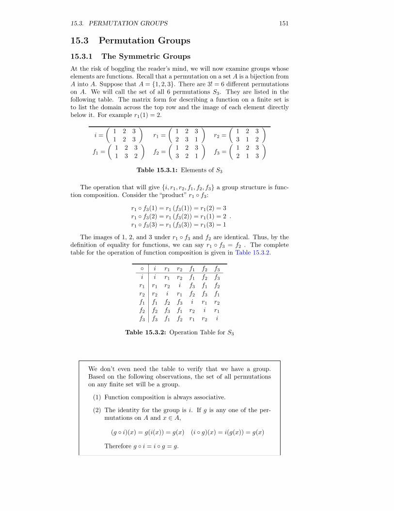
15.3. PERMUTATION GROUPS 151
15.3 Permutation Groups
15.3.1 The Symmetric GroupsAt the risk of boggling the reader’s mind, we will now examine groups whoseelements are functions. Recall that a permutation on a set A is a bijection fromA into A. Suppose that A = {1, 2, 3}. There are 3! = 6 different permutationson A. We will call the set of all 6 permutations S3. They are listed in thefollowing table. The matrix form for describing a function on a finite set isto list the domain across the top row and the image of each element directlybelow it. For example r1(1) = 2.
i =
(1 2 3
1 2 3
)r1 =
(1 2 3
2 3 1
)r2 =
(1 2 3
3 1 2
)f1 =
(1 2 3
1 3 2
)f2 =
(1 2 3
3 2 1
)f3 =
(1 2 3
2 1 3
)Table 15.3.1: Elements of S3
The operation that will give {i, r1, r2, f1, f2, f3} a group structure is func-tion composition. Consider the “product” r1 ◦ f3:
r1 ◦ f3(1) = r1 (f3(1)) = r1(2) = 3
r1 ◦ f3(2) = r1 (f3(2)) = r1(1) = 2
r1 ◦ f3(3) = r1 (f3(3)) = r1(3) = 1
.
The images of 1, 2, and 3 under r1 ◦ f3 and f2 are identical. Thus, by thedefinition of equality for functions, we can say r1 ◦ f3 = f2 . The completetable for the operation of function composition is given in Table 15.3.2.
◦ i r1 r2 f1 f2 f3
i i r1 r2 f1 f2 f3
r1 r1 r2 i f3 f1 f2
r2 r2 i r1 f2 f3 f1
f1 f1 f2 f3 i r1 r2
f2 f2 f3 f1 r2 i r1
f3 f3 f1 f2 r1 r2 i
Table 15.3.2: Operation Table for S3
We don’t even need the table to verify that we have a group.Based on the following observations, the set of all permutationson any finite set will be a group.
(1) Function composition is always associative.
(2) The identity for the group is i. If g is any one of the per-mutations on A and x ∈ A,
(g ◦ i)(x) = g(i(x)) = g(x) (i ◦ g)(x) = i(g(x)) = g(x)
Therefore g ◦ i = i ◦ g = g.
152 CHAPTER 15. GROUP THEORY AND APPLICATIONS
(3) A permutation, by definition, is a bijection. In Chapter 7 weproved that this implies that it must have an inverse and theinverse itself is a bijection and hence a permutation. Henceall elements of S3 have an inverse in S3. If a permutation isdisplayed in matrix form, its inverse can be obtained by ex-changing the two rows and rearranging the columns so thatthe top row is in order. The first step is actually sufficientto obtain the inverse, but the sorting of the top row makesit easier to recognize the inverse.
For example, let’s consider a typical permutation on
{1, 2, 3, 4, 5}, f =
(1 2 3 4 5
5 3 2 1 4
).
f−1 =
(5 3 2 1 4
1 2 3 4 5
)=
(1 2 3 4 5
4 3 2 5 1
).
List 15.3.3
Note 15.3.4. From Table 15.3.2, we can see that S3 is non-abelian. Remem-ber, non-abelian is the negation of abelian. The existence of two elements thatdon’t commute is sufficient to make a group non-abelian. In this group, r1 andf3 is one such pair: r1 ◦f3 = f2 while f3 ◦r1 = f1, so r1 ◦f3 6= f3 ◦r1. Caution:Don’t take this to mean that every pair of elements has to have this property.There are several pairs of elements in S3 that do commute. In fact, the identity,i, must commute with everything. Also every element must commute with itsinverse.
Definition 15.3.5 Symmetric Group. Let A be a nonempty set. The setof all permutations on A with the operation of function composition is calledthe symmetric group on A, denoted SA.
The cardinality of a finite set A is more significant than the elements, andwe will denote by Sn the symmetric group on any set of cardinality n, n ≥ 1.
Example 15.3.6 The significance of S3. Our opening example, S3, is thesmallest non-abelian group. For that reason, all of its proper subgroups areabelian: in fact, they are all cyclic. Figure 15.3.7 shows the Hasse diagram forthe subgroups of S3.
Figure 15.3.7: Lattice diagram of subgroups of S3
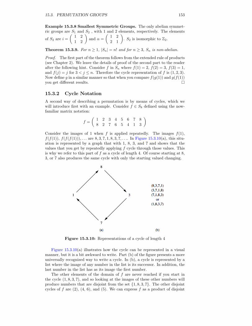
15.3. PERMUTATION GROUPS 153
Example 15.3.8 Smallest Symmetric Groups. The only abelian symmet-ric groups are S1 and S2 , with 1 and 2 elements, respectively. The elements
of S2 are i =
(1 2
1 2
)and α =
(1 2
2 1
). S2 is isomorphic to Z2.
Theorem 15.3.9. For n ≥ 1, |Sn| = n! and for n ≥ 3, Sn is non-abelian.
Proof. The first part of the theorem follows from the extended rule of products(see Chapter 2). We leave the details of proof of the second part to the readerafter the following hint. Consider f in Sn where f(1) = 2, f(2) = 3, f(3) = 1,and f(j) = j for 3 < j ≤ n. Therefore the cycle representation of f is (1, 2, 3).Now define g in a similar manner so that when you compare f(g(1)) and g(f(1))you get different results.
15.3.2 Cycle NotationA second way of describing a permutation is by means of cycles, which wewill introduce first with an example. Consider f ∈ S8 defined using the now-familiar matrix notation:
f =
(1 2 3 4 5 6 7 8
8 2 7 6 5 4 1 3
)Consider the images of 1 when f is applied repeatedly. The images f(1),f(f(1)), f(f(f(1))), . . . are 8, 3, 7, 1, 8, 3, 7, . . .. In Figure 15.3.10(a), this situ-ation is represented by a graph that with 1, 8, 3, and 7 and shows that thevalues that you get by repeatedly applying f cycle through those values. Thisis why we refer to this part of f as a cycle of length 4. Of course starting at 8,3, or 7 also produces the same cycle with only the starting valued changing.
Figure 15.3.10: Representations of a cycle of length 4
Figure 15.3.10(a) illustrates how the cycle can be represented in a visualmanner, but it is a bit awkward to write. Part (b) of the figure presents a moreuniversally recognized way to write a cycle. In (b), a cycle is represented by alist where the image of any number in the list is its successor. In addition, thelast number in the list has as its image the first number.
The other elements of the domain of f are never reached if you start inthe cycle (1, 8, 3, 7), and so looking at the images of these other numbers willproduce numbers that are disjoint from the set {1, 8, 3, 7}. The other disjointcycles of f are (2), (4, 6), and (5). We can express f as a product of disjoint
154 CHAPTER 15. GROUP THEORY AND APPLICATIONS
cycles: f = (1, 8, 3, 7)(2)(4, 6)(5) or f = (1, 8, 3, 7)(4, 6), where the absence of2 and 5 implies that f(2) = 2 and f(5) = 5.
Note 15.3.11 Disjoint Cycles. We say that two cycles are disjoint if nonumber appears in both cycles, as is the case in our expressions for f above.Disjoint cycles can be written in any order. Thus, we could also say thatf = (4, 6)(1, 8, 3, 7).
Note 15.3.12 Composition of Permutations. We will now consider thecomposition of permutations written in cyclic form by an example. Supposethat f = (1, 8, 3, 7)(4, 6) and g = (1, 5, 6)(8, 3, 7, 4) are elements of S8. Tocalculate f ◦ g, we start with simple concatenation:
f ◦ g = (1, 8, 3, 7)(4, 6)(1, 5, 6)(8, 3, 7, 4) (15.3.1)
Although this is a valid expression for f ◦ g, our goal is to express the com-position as a product of disjoint cycles as f and g were individually written.We will start by determining the cycle that contains 1. When combining anynumber of cycles, they are always read from right to left, as with all functions.The first cycle in (15.3.1) does not contain 1; thus we move on to the second.The image of 1 under that cycle is 5. Now we move on to the next cycle,looking for 5, which doesn’t appear. The fourth cycle does not contain a 5either; so f ◦ g(1) = 5.
At this point, we would have written “f ◦ g = (1, 5 ” on paper. We repeatthe steps to determine f ◦ g(5). This time the second cycle of (15.3.1) moves 5to 6 and then the third cycle moves 6 to 4. Therefore, f ◦g(5) = 4. We continueuntil the cycle (1, 5, 4, 3) is completed by determining that f ◦ g(3) = 1. Theprocess is then repeated starting with any number that does not appear in thecycle(s) that have already been completed.
The final result for our example is f ◦g = (1, 5, 4, 3)(6, 8, 7). Since f(2) = 2and g(2) = 2, f ◦ g(2) = 2 and we need not include the one-cycle (2) in thefinal result, although it can be included.
Example 15.3.13 Some Compositions.
(a) (1, 2, 3, 4)(1, 2, 3, 4) = (1, 3)(2, 4)
(b) (1, 4)(1, 3)(1, 2) = (1, 2, 3, 4).
Notice that cyclic notation does not indicate the set which is being permuted.The examples above could be in S5, where the image of 5 is 5. This ambiguityis usually overcome by making the context clear at the start of a discussion.
Definition 15.3.14 Transposition. A transposition is a cycle of length 2.
Observation 15.3.15 About transpositions. f = (1, 4) and g = (4, 5) aretranspositions in S5. However, f ◦ g = (1, 4, 5) and g ◦ f = (1, 5, 4) are nottranspositions; thus, the set of transpositions is not closed under composition.Since f2 = f ◦ f and g2 = g ◦ g are both equal to the identity permutation, fand g are their own inverses. In fact, every transposition is its own inverse.
Theorem 15.3.16 Decomposition into Cycles. Every cycle of length greaterthan 2 can be expressed as a product of transpositions.
Proof. We need only indicate how the product of transpositions can be ob-tained. It is easy to verify that a cycle of length k, (a1, a2, a3, . . . , ak), is equalto the following product of k − 1 transpositions:
(a1, ak) · · · (a1, a3) (a1, a2)
15.3. PERMUTATION GROUPS 155
Of course, a product of cycles can be written as a product of transpositionsjust as easily by applying the rule above to each cycle. For example,
(1, 3, 5, 7)(2, 4, 6) = (1, 7)(1, 5)(1, 3)(2, 6)(2, 4)
Unlike the situation with disjoint cycles, we are not free to change the orderof these transpositions.
15.3.3 Parity of Permutations and the Alternating GroupA decomposition of permutations into transpositions makes it possible to clas-sify then and identify an important family of groups.
The proofs of the following theorem appears in many abstract algebra texts.
Theorem 15.3.17. Every permutation on a finite set can be expressed as theproduct of an even number of transpositions or an odd number of transpositions,but not both.
Theorem 15.3.17 suggests that Sn can be partitioned into its “even” and“odd” elements. For example, the even permutations of S3 are i, r1 = (1, 2, 3) =(1, 3)(1, 2) and r2 = (1, 3, 2) = (1, 2)(1, 3). They form a subgroup, {i, r1, r2} ofS3.
In general:
Definition 15.3.18 The Alternating Group. Let n ≥ 2. The set of evenpermutations in Sn is a proper subgroup of Sn called the alternating group on{1, 2, . . . , n}, denoted An.
We justify our statement that An is a group:
Theorem 15.3.19. Let n ≥ 2. The alternating group is indeed a group andhas order n!
2 .
Proof. In this proof, the symbols si and ti stand for transpositions and p, q areeven nonnegative integers. If f, g ∈ An, we can write the two permutations asproducts of even numbers of transpositions, f = s1s2 · · · sp and g = t1t2 · · · tq.Then
f ◦ g = s1s2 · · · spt1t2 · · · tqSince p + q is even, f ◦ g ∈ An, and An is closed with respect to functioncomposition. With this, we have proven that An is a subgroup of Sn byTheorem 11.5.5.
To prove the final assertion, let Bn be the set of odd permutations and letτ = (1, 2). Define θ : An → Bn by θ(f) = f ◦ τ . Suppose that θ(f) = θ(g).Then f ◦ τ = g ◦ τ and by the right cancellation law, f = g. Hence, θ is aninjection. Next we show that θ is also a surjection. If h ∈ Bn, h is the imageof an element of An. Specifically, h is the image of h ◦ τ .
θ(h ◦ τ) = (h ◦ τ) ◦ τ= h ◦ (τ ◦ τ) Why?= h ◦ i Why?= h
Since θ is a bijection, |An| = |Bn| = n!2 .
Example 15.3.20 The Sliding Tile Puzzle. Consider the sliding-tile puz-zles pictured in Figure 15.3.21. Each numbered square is a tile and the dark
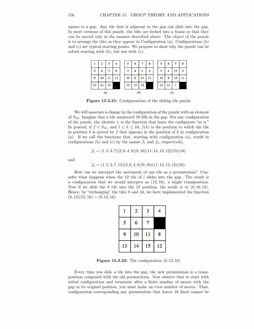
156 CHAPTER 15. GROUP THEORY AND APPLICATIONS
square is a gap. Any tile that is adjacent to the gap can slide into the gap.In most versions of this puzzle, the tiles are locked into a frame so that theycan be moved only in the manner described above. The object of the puzzleis to arrange the tiles as they appear in Configuration (a). Configurations (b)and (c) are typical starting points. We propose to show why the puzzle can besolved starting with (b), but not with (c).
Figure 15.3.21: Configurations of the sliding tile puzzle
We will associate a change in the configuration of the puzzle with an elementof S16. Imagine that a tile numbered 16 fills in the gap. For any configurationof the puzzle, the identity i, is the function that leave the configurate “as is.”In general, if f ∈ S16, and 1 ≤ k ≤ 16, f(k) is the position to which the tilein position k is moved by f that appears in the position of k in configuration(a). If we call the functions that, starting with configuration (a), result inconfigurations (b) and (c) by the names f1 and f2, respectively,
f1 = (1, 5, 3, 7)(2, 6, 4, 8)(9, 10)(11, 14, 13, 12)(15)(16)
andf2 = (1, 5, 3, 7, 15)(2, 6, 4, 8)(9, 10)(11, 14, 13, 12)(16).
How can we interpret the movement of one tile as a permutation? Con-sider what happens when the 12 tile of i slides into the gap. The result isa configuration that we would interpret as (12, 16), a single transposition.Now if we slide the 8 tile into the 12 position, the result is or (8, 16, 12).Hence, by “exchanging” the tiles 8 and 16, we have implemented the function(8, 12)(12, 16) = (8, 12, 16).
Figure 15.3.22: The configuration (8, 12, 16)
Every time you slide a tile into the gap, the new permutation is a trans-position composed with the old permutation. Now observe that to start withinitial configuration and terminate after a finite number of moves with thegap in its original position, you must make an even number of moves. Thus,configuration corresponding any permutation that leaves 16 fixed cannot be
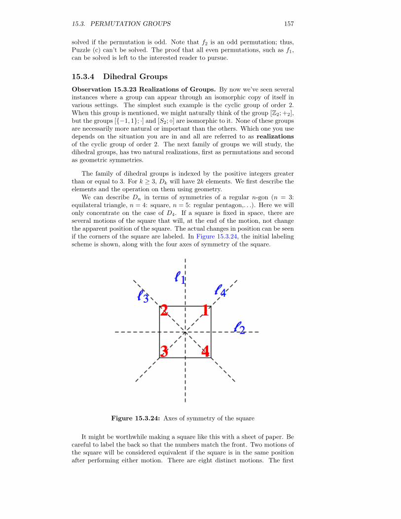
15.3. PERMUTATION GROUPS 157
solved if the permutation is odd. Note that f2 is an odd permutation; thus,Puzzle (c) can’t be solved. The proof that all even permutations, such as f1,can be solved is left to the interested reader to pursue.
15.3.4 Dihedral Groups
Observation 15.3.23 Realizations of Groups. By now we’ve seen severalinstances where a group can appear through an isomorphic copy of itself invarious settings. The simplest such example is the cyclic group of order 2.When this group is mentioned, we might naturally think of the group [Z2; +2],but the groups [{−1, 1}; ·] and [S2; ◦] are isomorphic to it. None of these groupsare necessarily more natural or important than the others. Which one you usedepends on the situation you are in and all are referred to as realizationsof the cyclic group of order 2. The next family of groups we will study, thedihedral groups, has two natural realizations, first as permutations and secondas geometric symmetries.
The family of dihedral groups is indexed by the positive integers greaterthan or equal to 3. For k ≥ 3, Dk will have 2k elements. We first describe theelements and the operation on them using geometry.
We can describe Dn in terms of symmetries of a regular n-gon (n = 3:equilateral triangle, n = 4: square, n = 5: regular pentagon,. . .). Here we willonly concentrate on the case of D4. If a square is fixed in space, there areseveral motions of the square that will, at the end of the motion, not changethe apparent position of the square. The actual changes in position can be seenif the corners of the square are labeled. In Figure 15.3.24, the initial labelingscheme is shown, along with the four axes of symmetry of the square.
Figure 15.3.24: Axes of symmetry of the square
It might be worthwhile making a square like this with a sheet of paper. Becareful to label the back so that the numbers match the front. Two motions ofthe square will be considered equivalent if the square is in the same positionafter performing either motion. There are eight distinct motions. The first
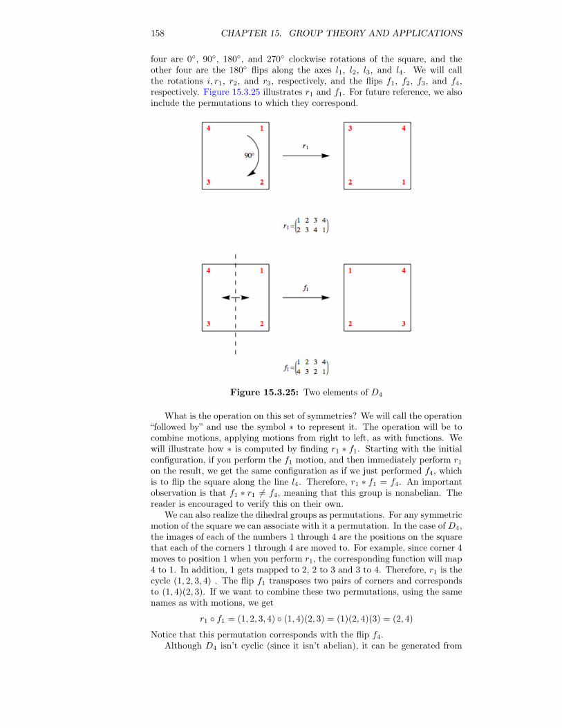
158 CHAPTER 15. GROUP THEORY AND APPLICATIONS
four are 0◦, 90◦, 180◦, and 270◦ clockwise rotations of the square, and theother four are the 180◦ flips along the axes l1, l2, l3, and l4. We will callthe rotations i, r1, r2, and r3, respectively, and the flips f1, f2, f3, and f4,respectively. Figure 15.3.25 illustrates r1 and f1. For future reference, we alsoinclude the permutations to which they correspond.
Figure 15.3.25: Two elements of D4
What is the operation on this set of symmetries? We will call the operation“followed by” and use the symbol ∗ to represent it. The operation will be tocombine motions, applying motions from right to left, as with functions. Wewill illustrate how ∗ is computed by finding r1 ∗ f1. Starting with the initialconfiguration, if you perform the f1 motion, and then immediately perform r1
on the result, we get the same configuration as if we just performed f4, whichis to flip the square along the line l4. Therefore, r1 ∗ f1 = f4. An importantobservation is that f1 ∗ r1 6= f4, meaning that this group is nonabelian. Thereader is encouraged to verify this on their own.
We can also realize the dihedral groups as permutations. For any symmetricmotion of the square we can associate with it a permutation. In the case of D4,the images of each of the numbers 1 through 4 are the positions on the squarethat each of the corners 1 through 4 are moved to. For example, since corner 4moves to position 1 when you perform r1, the corresponding function will map4 to 1. In addition, 1 gets mapped to 2, 2 to 3 and 3 to 4. Therefore, r1 is thecycle (1, 2, 3, 4) . The flip f1 transposes two pairs of corners and correspondsto (1, 4)(2, 3). If we want to combine these two permutations, using the samenames as with motions, we get
r1 ◦ f1 = (1, 2, 3, 4) ◦ (1, 4)(2, 3) = (1)(2, 4)(3) = (2, 4)
Notice that this permutation corresponds with the flip f4.Although D4 isn’t cyclic (since it isn’t abelian), it can be generated from
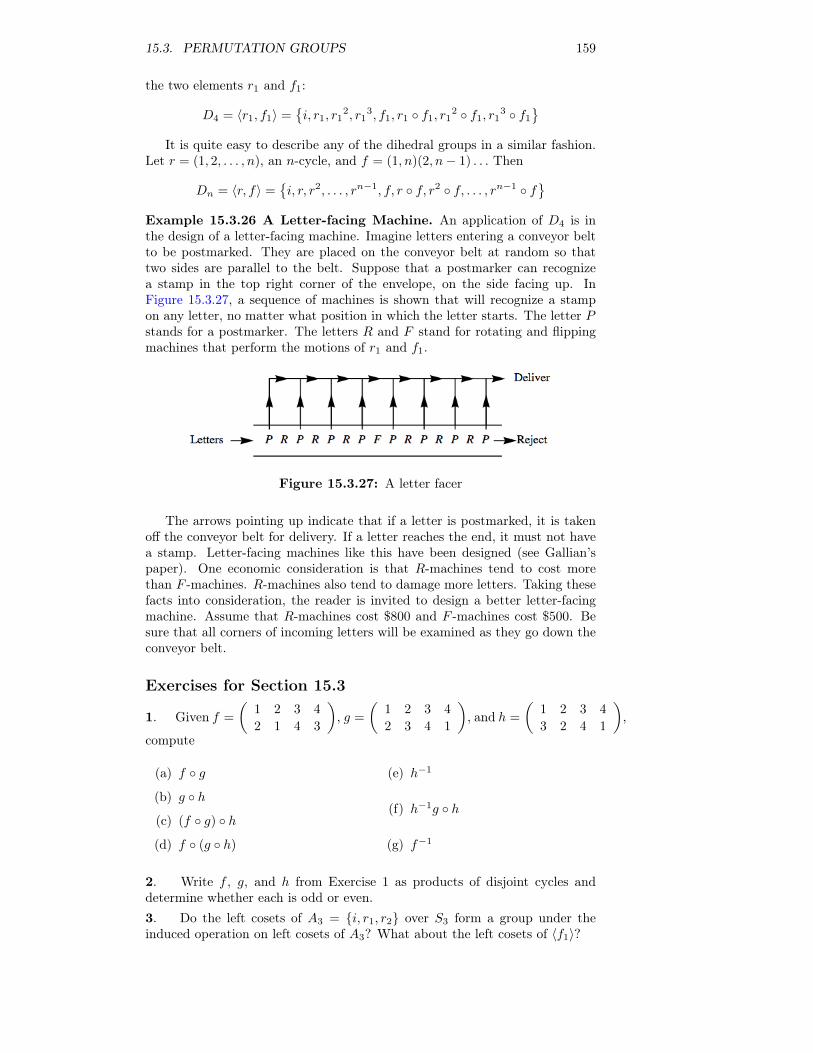
15.3. PERMUTATION GROUPS 159
the two elements r1 and f1:
D4 = 〈r1, f1〉 ={i, r1, r1
2, r13, f1, r1 ◦ f1, r1
2 ◦ f1, r13 ◦ f1
}It is quite easy to describe any of the dihedral groups in a similar fashion.
Let r = (1, 2, . . . , n), an n-cycle, and f = (1, n)(2, n− 1) . . . Then
Dn = 〈r, f〉 ={i, r, r2, . . . , rn−1, f, r ◦ f, r2 ◦ f, . . . , rn−1 ◦ f
}Example 15.3.26 A Letter-facing Machine. An application of D4 is inthe design of a letter-facing machine. Imagine letters entering a conveyor beltto be postmarked. They are placed on the conveyor belt at random so thattwo sides are parallel to the belt. Suppose that a postmarker can recognizea stamp in the top right corner of the envelope, on the side facing up. InFigure 15.3.27, a sequence of machines is shown that will recognize a stampon any letter, no matter what position in which the letter starts. The letter Pstands for a postmarker. The letters R and F stand for rotating and flippingmachines that perform the motions of r1 and f1.
Figure 15.3.27: A letter facer
The arrows pointing up indicate that if a letter is postmarked, it is takenoff the conveyor belt for delivery. If a letter reaches the end, it must not havea stamp. Letter-facing machines like this have been designed (see Gallian’spaper). One economic consideration is that R-machines tend to cost morethan F -machines. R-machines also tend to damage more letters. Taking thesefacts into consideration, the reader is invited to design a better letter-facingmachine. Assume that R-machines cost $800 and F -machines cost $500. Besure that all corners of incoming letters will be examined as they go down theconveyor belt.
Exercises for Section 15.3
1. Given f =
(1 2 3 4
2 1 4 3
), g =
(1 2 3 4
2 3 4 1
), and h =
(1 2 3 4
3 2 4 1
),
compute
(a) f ◦ g
(b) g ◦ h
(c) (f ◦ g) ◦ h
(d) f ◦ (g ◦ h)
(e) h−1
(f) h−1g ◦ h
(g) f−1
2. Write f , g, and h from Exercise 1 as products of disjoint cycles anddetermine whether each is odd or even.3. Do the left cosets of A3 = {i, r1, r2} over S3 form a group under theinduced operation on left cosets of A3? What about the left cosets of 〈f1〉?
160 CHAPTER 15. GROUP THEORY AND APPLICATIONS
4. In its realization as permutations, the dihedral group D3 is equal to S3.Can you give a geometric explanation why? Why isn’t D4 equal to S4?
5.
(a) Complete the list of elements of D4 and write out a table for the groupin its realization as symmetries.
(b) List the subgroups of D4 in a lattice diagram. Are they all cyclic? Towhat simpler groups are the subgroups of D4 isomorphic?
6. Design a better letter-facing machine (see Example 15.3.26). How canyou verify that a letter-facing machine does indeed check every corner of aletter? Can it be done on paper without actually sending letters through it?
7. Prove by induction that if r ≥ 1 and each ti, is a transposition, then(t1 ◦ t2 ◦ · · · ◦ tr)−1 = tr ◦ · · · ◦ t2 ◦ t18. How many elements are there in D5 ? Describe them geometrically.
9. Complete the proof of Theorem 15.3.9.
10. How many left cosets does An, n ≥ 2 have?
11. Prove that f ◦ r = rn−1 ◦ f in Dn.
12.
(a) Prove that the tile puzzles corresponding to A16 ∩{f ∈ S16| f(16) = 16}are solvable.
(b) If f(16) 6= 16, how can you determine whether f ’s puzzle is solvable?
13.
(a) Prove that S3 is isomorphic to R3, the group of 3× 3 rook matrices (seeSection 11.2 exercises).
(b) Prove that for each n ≥ 2, Rn is isomorphic to Sn.
15.4 Normal Subgroups and Group Homomor-phisms
Our goal in this section is to answer an open question from earlier in thischapter and introduce a related concept. The question is: When are left cosetsof a subgroup a group under the induced operation? This question is open fornon-abelian groups. Now that we have some examples to work with, we cantry a few experiments.
15.4.1 Normal Subgroups
Example 15.4.1 Cosets of A3. We have seen that A3 = {i, r1, r2} is asubgroup of S3, and its left cosets are A3 itself and B3 = {f1, f2, f3}. Whether{A3, B3} is a group boils down to determining whether the induced operationis well defined. Consider the operation table for S3 in Figure 15.4.2.
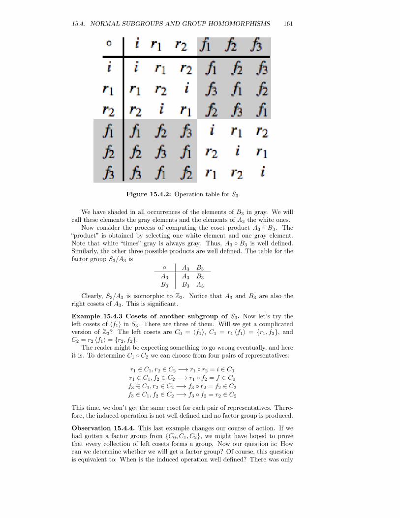
15.4. NORMAL SUBGROUPS AND GROUP HOMOMORPHISMS 161
Figure 15.4.2: Operation table for S3
We have shaded in all occurrences of the elements of B3 in gray. We willcall these elements the gray elements and the elements of A3 the white ones.
Now consider the process of computing the coset product A3 ◦ B3. The“product” is obtained by selecting one white element and one gray element.Note that white “times” gray is always gray. Thus, A3 ◦ B3 is well defined.Similarly, the other three possible products are well defined. The table for thefactor group S3/A3 is
◦ A3 B3
A3
B3
A3 B3
B3 A3
Clearly, S3/A3 is isomorphic to Z2. Notice that A3 and B3 are also theright cosets of A3. This is significant.
Example 15.4.3 Cosets of another subgroup of S3. Now let’s try theleft cosets of 〈f1〉 in S3. There are three of them. Will we get a complicatedversion of Z3? The left cosets are C0 = 〈f1〉, C1 = r1 〈f1〉 = {r1, f3}, andC2 = r2 〈f1〉 = {r2, f2}.
The reader might be expecting something to go wrong eventually, and hereit is. To determine C1 ◦ C2 we can choose from four pairs of representatives:
r1 ∈ C1, r2 ∈ C2 −→ r1 ◦ r2 = i ∈ C0
r1 ∈ C1, f2 ∈ C2 −→ r1 ◦ f2 = f ∈ C0
f3 ∈ C1, r2 ∈ C2 −→ f3 ◦ r2 = f2 ∈ C2
f3 ∈ C1, f2 ∈ C2 −→ f3 ◦ f2 = r2 ∈ C2
This time, we don’t get the same coset for each pair of representatives. There-fore, the induced operation is not well defined and no factor group is produced.
Observation 15.4.4. This last example changes our course of action. If wehad gotten a factor group from {C0, C1, C2}, we might have hoped to provethat every collection of left cosets forms a group. Now our question is: Howcan we determine whether we will get a factor group? Of course, this questionis equivalent to: When is the induced operation well defined? There was only
162 CHAPTER 15. GROUP THEORY AND APPLICATIONS
one step in the proof of Theorem 15.2.18, where we used the fact that G wasabelian. We repeat the equations here:
a′ ∗ b′ = (a ∗ h1) ∗ (b ∗ h2) = (a ∗ b) ∗ (h1 ∗ h2)
since G was abelian.The last step was made possible by the fact that h1∗b = b∗h1. As the proof
continued, we used the fact that h1 ∗ h2 was in H and so a′ ∗ b′ is (a ∗ b) ∗ hfor some h in H. All that we really needed in the “abelian step” was thath1 ∗ b = b ∗ (something in H) = b ∗ h3. Then, since H is closed under G’soperation, h3 ∗ h2 is an element of H. The consequence of this observation isthat we define a certain kind of subgroup that guarantees that the inductedoperation is well-defined.
Definition 15.4.5 Normal Subgroup. If G is a group, H ≤ G, then H is anormal subgroup of G, denoted H /G, if and only if every left coset of H is aright coset of H; i. e. a ∗H = H ∗ a ∀a ∈ G
Theorem 15.4.6. If H ≤ G, then the operation induced on left cosets of Hby the operation of G is well defined if and only if any one of the followingconditions is true:
(a) H is a normal subgroup of G.
(b) If h ∈ H, a ∈ G, then there exists h′ ∈ H such that h ∗ a = a ∗ h′.
(c) If h ∈ H, a ∈ G, then a−1 ∗ h ∗ a ∈ H.
Proof. We leave the proof of this theorem to the reader.
Be careful, the following corollary is not an “...if and only if...” statement.
Corollary 15.4.7. If H ≤ G, then the operation induced on left cosets of Hby the operation of G is well defined if either of the following two conditions istrue.
(a) G is abelian.
(b) |H| = |G|2 .
Example 15.4.8 A non-normal subgroup. The right cosets of 〈f1〉 ≤ S3
are {i, f1}, {r1f2}, and {r2, f3}. These are not the same as the left cosets of〈f1〉. In addition, f2
−1f1f2 = f2f1f2 = f3 /∈ 〈f1〉. Thus, 〈f1〉 is not normal.
The improper subgroups {e} and G of any group G are normal subgroups.G/{e} is isomorphic to G. All other normal subgroups of a group, if they exist,are called proper normal subgroups.
Example 15.4.9. By Condition b of Corollary 15.4.7, An is a normal sub-group of Sn and Sn/An is isomorphic to Z2.
Example 15.4.10 Subgroups of A5. A5, a group in its own right with 60elements, has many proper subgroups, but none are normal. Although thiscould be done by brute force, the number of elements in the group would makethe process tedious. A far more elegant way to approach the verification of thisstatement is to use the following fact about the cycle structure of permutations.If f ∈ Sn is a permutation with a certain cycle structure, σ1σ2 · · ·σk, where thelength of σi is `i, then for any g ∈ Sn, g−1◦f ◦g, which is the conjugate of f by
15.4. NORMAL SUBGROUPS AND GROUP HOMOMORPHISMS 163
g, will have a cycle structure with exactly the same cycle lengths. For exampleif we take f = (1, 2, 3, 4)(5, 6)(7, 8, 9) ∈ S9 and conjugate by g = (1, 3, 5, 7, 9),
g−1 ◦ f ◦ g = (1, 9, 7, 5, 3) ◦ (1, 2, 3, 4)(5, 6)(7, 8, 9) ◦ (1, 3, 5, 7, 9)
= (1, 4, 9, 2)(3, 6)(5, 8, 7)
Notice that the condition for normality of a subgroup H of G is that theconjugate of any element of H by an element of G must be remain in H.
To verify that A5 has no proper normal subgroups, you can start by cata-loging the different cycle structures that occur in A5 and how many elementshave those structures. Then consider what happens when you conjugate thesedifferent cycle structures with elements of A5. An outline of the process is inthe exercises.
Example 15.4.11. Let G be the set of two by two invertible matrices of realnumbers. That is,
G =
{(a b
c d
)| a, b, c, d ∈ R, ad− bc 6= 0
}We saw in Chapter 11 that G is a group with matrix multiplication.
This group has many subgroups, but consider just two: H1 =
{(a 0
0 a
)∣∣∣∣ a 6= 0
}and H2 =
{(a 0
0 d
)∣∣∣∣ ad 6= 0
}. It is fairly simple to apply one of the condi-
tions we have observed for normallity that H1 a normal subgroup of G, whileH2 is not normal in G.
15.4.2 HomomorphismsThink of the word isomorphism. Chances are, one of the first images thatcomes to mind is an equation something like
θ(x ∗ y) = θ(x) � θ(y)
An isomorphism must be a bijection, but the equation above is the algebraicproperty of an isomorphism. Here we will examine functions that satisfy equa-tions of this type.
Definition 15.4.12 Homomorphism. Let [G; ∗] and [G′; �] be groups. θ :G→ G′ is a homomorphism if θ(x ∗ y) = θ(x) � θ(y) for all x, y ∈ G.
Many homomorphisms are useful since they point out similarities betweenthe two groups (or, on the universal level, two algebraic systems) involved.
Example 15.4.13 Decreasing modularity. Define α : Z6 → Z3 by α(n) =n mod 3. Therefore, α(0) = 0, α(1) = 1, α(2) = 2, α(3) = 1 + 1 + 1 = 0,α(4) = 1, and α(5) = 2. If n,m ∈ Z6. We could actually show that α is ahomomorphism by checking all 62 = 36 different cases for the formula
α(n+6 m) = α(n) +3 α(m) (15.4.1)
but we will use a line of reasoning that generalizes. We have already en-countered the Chinese Remainder Theorem, which implies that the functionβ : Z6 → Z3×Z2 defined by β(n) = (n mod 3, n mod 2). We need only observethat equating the first coordinates of both sides of the equation
β(n+6 m) = β(n) +3 β(m) (15.4.2)
gives us precisely the homomorphism property.
164 CHAPTER 15. GROUP THEORY AND APPLICATIONS
Theorem 15.4.14 Group Homomorphism Properties. If θ : G → G′ isa homomorphism, then:
(a) θ(e) = θ(the identity of G) = the identity of G′ = e′.
(b) θ(a−1
)= θ(a)−1 for all a ∈ G.
(c) If H ≤ G, then θ(H) = {θ(h)|h ∈ H} ≤ G′.
Proof.
(a) Let a be any element of G. Then θ(a) ∈ G′.
θ(a) � e′ = θ(a) by the definition of e′
= θ(a ∗ e) by the definition of e= θ(a) � θ(e) by the fact that θ is a homomorphism
By cancellation, e′ = θ(e).
(b) Again, let a ∈ G. e′ = θ(e) = θ(a ∗ a−1
)= θ(a) � θ
(a−1
). Hence, by the
uniqueness of inverses, θ(a)−1 = θ(a−1
).
(c) Let b1, b2 ∈ θ(H). Then there exists a1, a2 ∈ H such that θ (a1) = b1,θ (a2) = b2. Recall that a compact necessary and sufficient condition forH ≤ G is that x ∗ y−1 ∈ H for all x, y ∈ H. Now we apply the samecondition in G′:
b1 � b2−1 = θ (a1) � θ (a2)−1
= θ (a1) � θ(a2−1)
= θ(a1 ∗ a2
−1)∈ θ(H)
since a1 ∗ a2−1 ∈ H, and so we can conclude that θ(H) ≤ G′.
Corollary 15.4.15. Since a homomorphism need not be a surjection and part(c) of Theorem 15.4.14 is true for the case of H = G, the range of θ, θ(G), isa subgroup of G′
Example 15.4.16. If we define π : Z→ Z/4Z by π(n) = n+ 4Z, then π is ahomomorphism. The image of the subgroup 4Z is the single coset 0 + 4Z, theidentity of the factor group. Homomorphisms of this type are called naturalhomomorphisms. The following theorems will verify that π is a homomorphismand also show the connection between homomorphisms and normal subgroups.The reader can find more detail and proofs in most abstract algebra texts.
Theorem 15.4.17. If H / G, then the function π : G → G/H defined byπ(a) = aH is a homomorphism.
Proof. We leave the proof of this theorem to the reader.
Definition 15.4.18 Natural Homomorphism. If H /G, then the functionπ : G→ G/H defined by π(a) = aH is called the natural homomorphism.
Based on Theorem 15.4.17, every normal subgroup gives us a homomor-phism. Next, we see that the converse is true.
Definition 15.4.19 Kernel of a homomorphism. Let θ : G → G′ be ahomomorphism, and let e and e′ be the identitites of G and G′, respectively.The kernel of θ is the set ker θ = {a ∈ G | θ(a) = e′}
15.4. NORMAL SUBGROUPS AND GROUP HOMOMORPHISMS 165
Theorem 15.4.20. Let θ : G→ G′ be a homomorphism from G into G′ . Thekernel of θ is a normal subgroup of G.
Proof. Let K = ker θ. We can see that K is a subgroup of G by lettinga, b ∈ K and verify that a∗ b−1 ∈ K by computing θ(a∗ b−1) = θ(a)∗ θ(b)−1 =e′ ∗ e′−1 = e′. To prove normality, we let g be any element of G and k ∈ K.We compute θ(g ∗ k ∗ g−1) to verify that g ∗ k ∗ g−1 ∈ K.
θ(g ∗ k ∗ g−1) = θ(g) ∗ θ(k) ∗ θ(g−1)
= θ(g) ∗ θ(k) ∗ θ(g)−1
= θ(g) ∗ e′ ∗ θ(g)−1
= θ(g) ∗ θ(g)−1
= e′
Based on this most recent theorem, every homomorphism gives us a normalsubgroup.
Theorem 15.4.21 Fundamental Theorem of Group Homomorphisms.Let θ : G→ G′ be a homomorphism. Then θ(G) is isomorphic to G/ ker θ.
Example 15.4.22. Define θ : Z → Z10 by θ(n) = n mod 10. The threeprevious theorems imply the following:
• π : Z→ Z/10Z defined by π(n) = n+ 10Z is a homomorphism.
• {n ∈ Z|θ(n) = 0} = {10n | n ∈ Z} = 10Z / Z.
• Z/10Z is isomorphic to Z10.
Example 15.4.23. Let G be the same group of two by two invertible realmatrices as in Example 15.4.11. Define Φ : G → G by Φ(A) = A√
|detA|. We
will let the reader verify that Φ is a homomorphism. The theorems aboveimply the following.
• ker Φ = {A ∈ G|Φ(A) = I} =
{(a 0
0 a
)| a ∈ R, a 6= 0
}/ G. This
verifies our statement in Example 15.4.11. As in that example, let ker Φ =H1.
• G /H1 is isomorphic to {A ∈ G | detA = 1}.
• π : G→ G /H1 defined, naturally, by π(A) = AH1 is a homomorphism.
For the remainder of this section, we will be examining certain kinds ofhomomorphisms that will play a part in our major application to homomor-phisms, coding theory.
Example 15.4.24. Consider Φ : Z22 → Z2
3 defined by Φ(a, b) = (a, b, a+2 b).If (a1, b1) , (a2, b2) ∈ Z2
2,
Φ ((a1, b1) + (a2, b2)) = Φ (a1 +2 a2, b1 +2 b2)
= (a1 +2 a2, b1 +2 b2, a1 +2 a2 +2 b1 +2 b2)
= (a1, b1, a1 +2 b1) + (a2, b2, a2 +2 b2)
= Φ (a1, b1) + Φ (a2, b2)
Since Φ(a, b)=(0, 0, 0) implies that a = 0 and b = 0, the kernel of Φ is{(0, 0)}. By previous theorems, Φ
(Z2
2)
= {(0, 0, 0), (1, 0, 1), (0, 1, 1), (1, 1, 0)}is isomorphic to Z2
2.
166 CHAPTER 15. GROUP THEORY AND APPLICATIONS
We can generalize the previous example as follows: If n,m ≥ 1 and A is anm× n matrix of 0’s and 1’s (elements of Z2), then Φ : Z2
m → Z2n defined by
Φ (a1, a2, ..., am) = (a1, a2, ..., am)A
is a homomorphism. This is true because matrix multiplication is distributiveover addition. The only new idea here is that computation is done in Z2. Ifa = (a1, a2, ..., am) and b = (b1, b2, ..., bm), (a+ b)A = aA+ bA is true by basicmatrix laws. Therefore, Φ(a+ b) = Φ(a) + Φ(b).
Exercises for Section 15.41. Which of the following functions are homomorphisms? What are thekernels of those functions that are homomorphisms?
(a) θ1 : R∗ → R+ defined by θ1(a) = |a|.
(b) θ2 : Z5 → Z2 where θ2(n) =
{0 if n is even1 if n is odd
.
(c) θ3 : R× R→ R, where θ3(a, b) = a+ b.
(d) θ4 : S4 → S4 defined by θ4(f) = f ◦ f = f2.
2. Which of the following functions are homomorphisms? What are thekernels of those functions that are homomorphisms?
(a) α1 : M2×2(R)→ R, defined by α1(A) = A11A22 +A12A21.
(b) α2 : (R∗)2 → R∗ defined by α2(a, b) = ab.
(c) α3 : {A ∈M2×2(R)|detA 6= 0} → R∗, where α3(A) = detA.
(d) α4 : S4 → S4 defined by α4(f) = f−1.
3. Show that D4 has one proper normal subgroup, but that 〈(1, 4)(2, 3)〉 isnot normal.4. Prove that the function Φ in Example 15.4.23 is a homomorphism.5. Define the two functions α : Z2
3 → Z24 and β : Z2
4 → Z2 by α (a1, a2, a3) =(a1, a2, a3, a1 +2 a2 +2 a3), and β (b1, b2, b3, b4) = b1 + b2 + b3 + b4 Describe thefunction β ◦ α. Is it a homomorphism?6. Express Φ in Example 15.4.23 in matrix form.7. Prove that if G is an abelian group, then q(x) = x2 defines a homomor-phism from G into G. Is q ever an isomorphism?8. Prove that if θ : G→ G′ is a homomorphism, and H/G, then θ(H)/θ(G).Is it also true that θ(H) / G′?9. Prove that if θ : G → G′ is a homomorphism, and H ′ ≤ θ(G), thenθ−1(H ′) = {a ∈ G|θ(a) ∈ H ′} ≤ G.10. Following up on Example 15.4.10, prove that A5 is a simple group; i. e.,it has no proper normal subgroups.
(a) Make a list of the different cycle structures that occur in A5 and howmany elements have those structures.
(b) Within each set of permutations with different cycle structures, identifywhich subsets are closed with respect to the conjugation operation. Withthis you will have a partition of A5 into conjugate classes. where for eachclass C, f, g ∈ C if and only if ∃φ ∈ A5 such that φ−1 ◦ f ◦ φ = g.
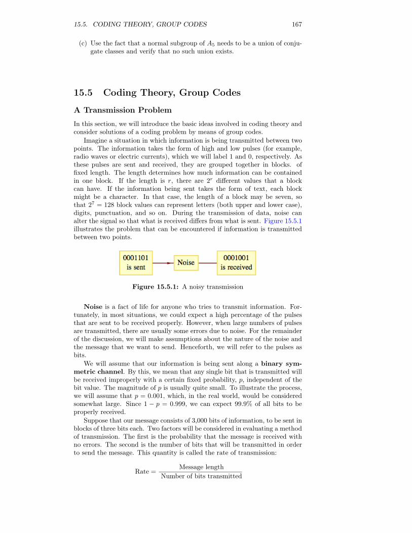
15.5. CODING THEORY, GROUP CODES 167
(c) Use the fact that a normal subgroup of A5 needs to be a union of conju-gate classes and verify that no such union exists.
15.5 Coding Theory, Group Codes
A Transmission Problem
In this section, we will introduce the basic ideas involved in coding theory andconsider solutions of a coding problem by means of group codes.
Imagine a situation in which information is being transmitted between twopoints. The information takes the form of high and low pulses (for example,radio waves or electric currents), which we will label 1 and 0, respectively. Asthese pulses are sent and received, they are grouped together in blocks. offixed length. The length determines how much information can be containedin one block. If the length is r, there are 2r different values that a blockcan have. If the information being sent takes the form of text, each blockmight be a character. In that case, the length of a block may be seven, sothat 27 = 128 block values can represent letters (both upper and lower case),digits, punctuation, and so on. During the transmission of data, noise canalter the signal so that what is received differs from what is sent. Figure 15.5.1illustrates the problem that can be encountered if information is transmittedbetween two points.
Figure 15.5.1: A noisy transmission
Noise is a fact of life for anyone who tries to transmit information. For-tunately, in most situations, we could expect a high percentage of the pulsesthat are sent to be received properly. However, when large numbers of pulsesare transmitted, there are usually some errors due to noise. For the remainderof the discussion, we will make assumptions about the nature of the noise andthe message that we want to send. Henceforth, we will refer to the pulses asbits.
We will assume that our information is being sent along a binary sym-metric channel. By this, we mean that any single bit that is transmitted willbe received improperly with a certain fixed probability, p, independent of thebit value. The magnitude of p is usually quite small. To illustrate the process,we will assume that p = 0.001, which, in the real world, would be consideredsomewhat large. Since 1 − p = 0.999, we can expect 99.9% of all bits to beproperly received.
Suppose that our message consists of 3,000 bits of information, to be sent inblocks of three bits each. Two factors will be considered in evaluating a methodof transmission. The first is the probability that the message is received withno errors. The second is the number of bits that will be transmitted in orderto send the message. This quantity is called the rate of transmission:
Rate =Message length
Number of bits transmitted
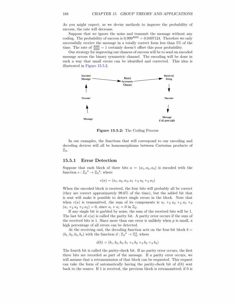
168 CHAPTER 15. GROUP THEORY AND APPLICATIONS
As you might expect, as we devise methods to improve the probability ofsuccess, the rate will decrease.
Suppose that we ignore the noise and transmit the message without anycoding. The probability of success is 0.9993000 = 0.0497124. Therefore we onlysuccessfully receive the message in a totally correct form less than 5% of thetime. The rate of 3000
3000 = 1 certainly doesn’t offset this poor probability.Our strategy for improving our chances of success will be to send an encoded
message across the binary symmetric channel. The encoding will be done insuch a way that small errors can be identified and corrected. This idea isillustrated in Figure 15.5.2.
Figure 15.5.2: The Coding Process
In our examples, the functions that will correspond to our encoding anddecoding devices will all be homomorphisms between Cartesian products ofZ2.
15.5.1 Error DetectionSuppose that each block of three bits a = (a1, a2, a3) is encoded with thefunction e : Z2
3 → Z24, where
e(a) = (a1, a2, a3, a1 +2 a2 +2 a3)
When the encoded block is received, the four bits will probably all be correct(they are correct approximately 99.6% of the time), but the added bit thatis sent will make it possible to detect single errors in the block. Note thatwhen e(a) is transmitted, the sum of its components is a1 +2 a2 +2 a3 +2
(a1 +2 a2 +2 a3) = 0, since ai + ai = 0 in Z2.If any single bit is garbled by noise, the sum of the received bits will be 1.
The last bit of e(a) is called the parity bit. A parity error occurs if the sum ofthe received bits is 1. Since more than one error is unlikely when p is small, ahigh percentage of all errors can be detected.
At the receiving end, the decoding function acts on the four-bit block b =(b1, b2, b3, b4) with the function d : Z2
4 → Z42, where
d(b) = (b1, b2, b3, b1 +2 b2 +2 b3 +2 b4)
The fourth bit is called the parity-check bit. If no parity error occurs, the firstthree bits are recorded as part of the message. If a parity error occurs, wewill assume that a retransmission of that block can be requested. This requestcan take the form of automatically having the parity-check bit of d(b) sentback to the source. If 1 is received, the previous block is retransmitted; if 0 is
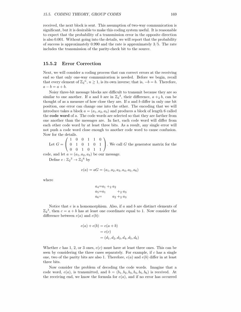
15.5. CODING THEORY, GROUP CODES 169
received, the next block is sent. This assumption of two-way communication issignificant, but it is desirable to make this coding system useful. It is reasonableto expect that the probability of a transmission error in the opposite directionis also 0.001. Without going into the details, we will report that the probabilityof success is approximately 0.990 and the rate is approximately 3/5. The rateincludes the transmission of the parity-check bit to the source.
15.5.2 Error Correction
Next, we will consider a coding process that can correct errors at the receivingend so that only one-way communication is needed. Before we begin, recallthat every element of Z2
n, n ≥ 1, is its own inverse; that is, −b = b. Therefore,a− b = a+ b.
Noisy three-bit message blocks are difficult to transmit because they are sosimilar to one another. If a and b are in Z2
3, their difference, a +2 b, can bethought of as a measure of how close they are. If a and b differ in only one bitposition, one error can change one into the other. The encoding that we willintroduce takes a block a = (a1, a2, a3) and produces a block of length 6 calledthe code word of a. The code words are selected so that they are farther fromone another than the messages are. In fact, each code word will differ fromeach other code word by at least three bits. As a result, any single error willnot push a code word close enough to another code word to cause confusion.Now for the details.
Let G =
1 0 0 1 1 0
0 1 0 1 0 1
0 0 1 0 1 1
. We call G the generator matrix for the
code, and let a = (a1, a2, a3) be our message.Define e : Z2
3 → Z26 by
e(a) = aG = (a1, a2, a3, a4, a5, a6)
where
a4=a1 +2 a2
a5=a1 +2 a3
a6= a2 +2 a3
Notice that e is a homomorphism. Also, if a and b are distinct elements ofZ2
3, then c = a + b has at least one coordinate equal to 1. Now consider thedifference between e(a) and e(b):
e(a) + e(b) = e(a+ b)
= e(c)
= (d1, d2, d3, d4, d5, d6)
Whether c has 1, 2, or 3 ones, e(c) must have at least three ones. This can beseen by considering the three cases separately. For example, if c has a singleone, two of the parity bits are also 1. Therefore, e(a) and e(b) differ in at leastthree bits.
Now consider the problem of decoding the code words. Imagine that acode word, e(a), is transmitted, and b = (b1, b2, b3, b4, b5, b6) is received. Atthe receiving end, we know the formula for e(a), and if no error has occurred
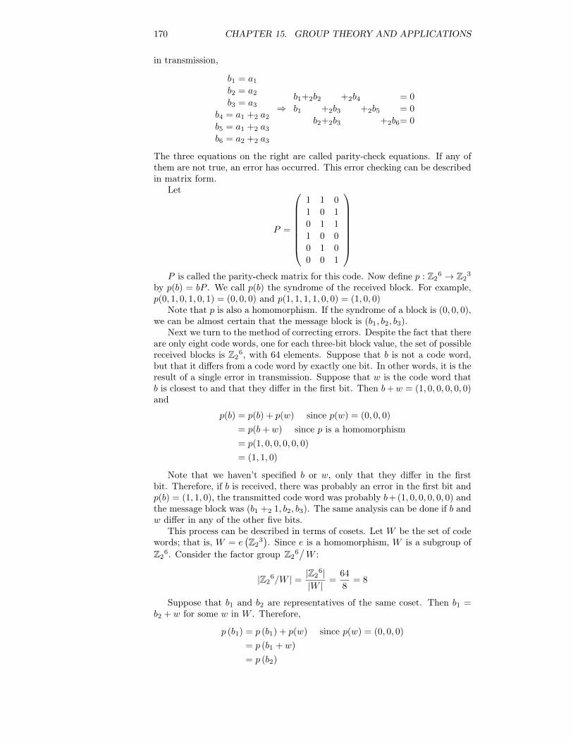
170 CHAPTER 15. GROUP THEORY AND APPLICATIONS
in transmission,
b1 = a1
b2 = a2
b3 = a3
b4 = a1 +2 a2
b5 = a1 +2 a3
b6 = a2 +2 a3
⇒b1+2b2 +2b4 = 0
b1 +2b3 +2b5 = 0
b2+2b3 +2b6= 0
The three equations on the right are called parity-check equations. If any ofthem are not true, an error has occurred. This error checking can be describedin matrix form.
Let
P =
1 1 0
1 0 1
0 1 1
1 0 0
0 1 0
0 0 1
P is called the parity-check matrix for this code. Now define p : Z2
6 → Z23
by p(b) = bP . We call p(b) the syndrome of the received block. For example,p(0, 1, 0, 1, 0, 1) = (0, 0, 0) and p(1, 1, 1, 1, 0, 0) = (1, 0, 0)
Note that p is also a homomorphism. If the syndrome of a block is (0, 0, 0),we can be almost certain that the message block is (b1, b2, b3).
Next we turn to the method of correcting errors. Despite the fact that thereare only eight code words, one for each three-bit block value, the set of possiblereceived blocks is Z2
6, with 64 elements. Suppose that b is not a code word,but that it differs from a code word by exactly one bit. In other words, it is theresult of a single error in transmission. Suppose that w is the code word thatb is closest to and that they differ in the first bit. Then b+w = (1, 0, 0, 0, 0, 0)and
p(b) = p(b) + p(w) since p(w) = (0, 0, 0)
= p(b+ w) since p is a homomorphism= p(1, 0, 0, 0, 0, 0)
= (1, 1, 0)
Note that we haven’t specified b or w, only that they differ in the firstbit. Therefore, if b is received, there was probably an error in the first bit andp(b) = (1, 1, 0), the transmitted code word was probably b+ (1, 0, 0, 0, 0, 0) andthe message block was (b1 +2 1, b2, b3). The same analysis can be done if b andw differ in any of the other five bits.
This process can be described in terms of cosets. Let W be the set of codewords; that is, W = e
(Z2
3). Since e is a homomorphism, W is a subgroup of
Z26. Consider the factor group Z2
6/W :
|Z26/W | = |Z2
6||W |
=64
8= 8
Suppose that b1 and b2 are representatives of the same coset. Then b1 =b2 + w for some w in W . Therefore,
p (b1) = p (b1) + p(w) since p(w) = (0, 0, 0)
= p (b1 + w)
= p (b2)
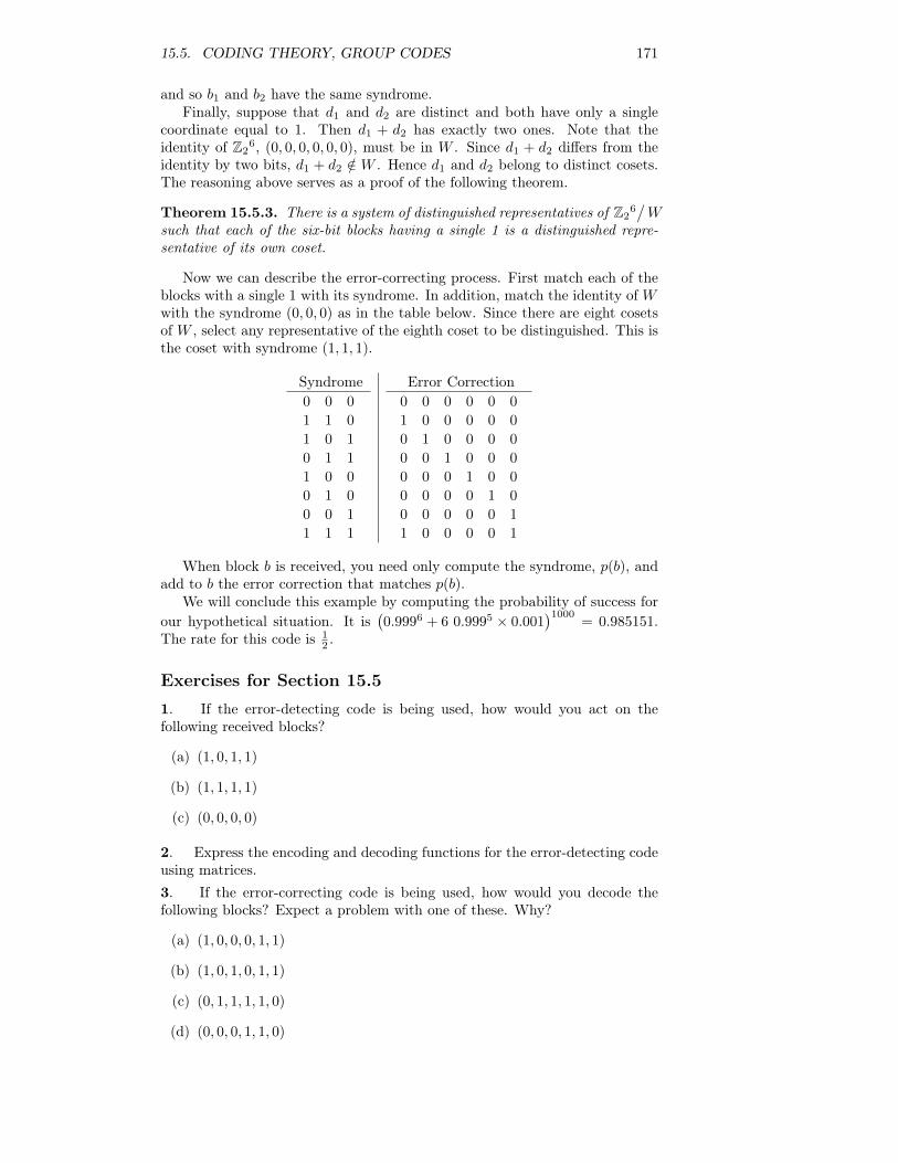
15.5. CODING THEORY, GROUP CODES 171
and so b1 and b2 have the same syndrome.Finally, suppose that d1 and d2 are distinct and both have only a single
coordinate equal to 1. Then d1 + d2 has exactly two ones. Note that theidentity of Z2
6, (0, 0, 0, 0, 0, 0), must be in W . Since d1 + d2 differs from theidentity by two bits, d1 + d2 /∈ W . Hence d1 and d2 belong to distinct cosets.The reasoning above serves as a proof of the following theorem.
Theorem 15.5.3. There is a system of distinguished representatives of Z26/W
such that each of the six-bit blocks having a single 1 is a distinguished repre-sentative of its own coset.
Now we can describe the error-correcting process. First match each of theblocks with a single 1 with its syndrome. In addition, match the identity of Wwith the syndrome (0, 0, 0) as in the table below. Since there are eight cosetsof W , select any representative of the eighth coset to be distinguished. This isthe coset with syndrome (1, 1, 1).
Syndrome0 0 0
1 1 0
1 0 1
0 1 1
1 0 0
0 1 0
0 0 1
1 1 1
Error Correction0 0 0 0 0 0
1 0 0 0 0 0
0 1 0 0 0 0
0 0 1 0 0 0
0 0 0 1 0 0
0 0 0 0 1 0
0 0 0 0 0 1
1 0 0 0 0 1
When block b is received, you need only compute the syndrome, p(b), andadd to b the error correction that matches p(b).
We will conclude this example by computing the probability of success forour hypothetical situation. It is
(0.9996 + 6 0.9995 × 0.001
)1000= 0.985151.
The rate for this code is 12 .
Exercises for Section 15.5
1. If the error-detecting code is being used, how would you act on thefollowing received blocks?
(a) (1, 0, 1, 1)
(b) (1, 1, 1, 1)
(c) (0, 0, 0, 0)
2. Express the encoding and decoding functions for the error-detecting codeusing matrices.3. If the error-correcting code is being used, how would you decode thefollowing blocks? Expect a problem with one of these. Why?
(a) (1, 0, 0, 0, 1, 1)
(b) (1, 0, 1, 0, 1, 1)
(c) (0, 1, 1, 1, 1, 0)
(d) (0, 0, 0, 1, 1, 0)
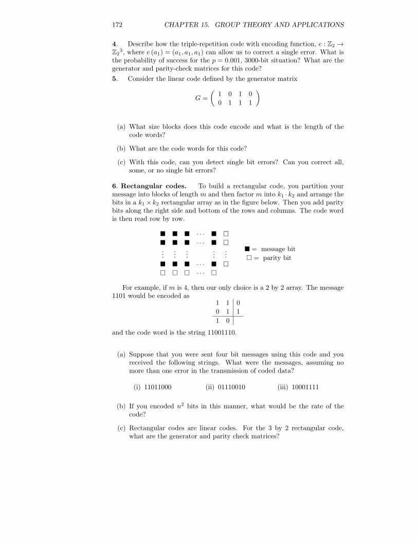
172 CHAPTER 15. GROUP THEORY AND APPLICATIONS
4. Describe how the triple-repetition code with encoding function, e : Z2 →Z2
3, where e (a1) = (a1, a1, a1) can allow us to correct a single error. What isthe probability of success for the p = 0.001, 3000-bit situation? What are thegenerator and parity-check matrices for this code?5. Consider the linear code defined by the generator matrix
G =
(1 0 1 0
0 1 1 1
)
(a) What size blocks does this code encode and what is the length of thecode words?
(b) What are the code words for this code?
(c) With this code, can you detect single bit errors? Can you correct all,some, or no single bit errors?
6. Rectangular codes. To build a rectangular code, you partition yourmessage into blocks of length m and then factor m into k1 · k2 and arrange thebits in a k1× k2 rectangular array as in the figure below. Then you add paritybits along the right side and bottom of the rows and columns. The code wordis then read row by row.
� � � · · · � �� � � · · · � �...
......
......
� � � · · · � �� � � · · · �
� = message bit� = parity bit
For example, if m is 4, then our only choice is a 2 by 2 array. The message1101 would be encoded as
1 1 0
0 1 1
1 0
and the code word is the string 11001110.
(a) Suppose that you were sent four bit messages using this code and youreceived the following strings. What were the messages, assuming nomore than one error in the transmission of coded data?
(i) 11011000 (ii) 01110010 (iii) 10001111
(b) If you encoded n2 bits in this manner, what would be the rate of thecode?
(c) Rectangular codes are linear codes. For the 3 by 2 rectangular code,what are the generator and parity check matrices?
Chapter 16
An Introduction to Rings andFields
In our early elementary school days we began the study of mathematics bylearning addition and multiplication on the set of positive integers. We thenextended this to operations on the set of all integers. Subtraction and divisionare defined in terms of addition and multiplication. Later we investigated theset of real numbers under the operations of addition and multiplication. Hence,it is quite natural to investigate those structures on which we can define thesetwo fundamental operations, or operations similar to them. The structuressimilar to the set of integers are called rings, and those similar to the set ofreal numbers are called fields.
In coding theory, highly structured codes are needed for speed and accuracy.The theory of finite fields is essential in the development of many structuredcodes. We will discuss basic facts about finite fields and introduce the readerto polynomial algebra.
16.1 Rings, Basic Definitions and Concepts
16.1.1 Basic Definitions
We would like to investigate algebraic systems whose structure imitates thatof the integers.
Definition 16.1.1 Ring. A ring is a set R together with two binary opera-tions, addition and multiplication, denoted by the symbols + and · such thatthe following axioms are satisfied:
(1) [R; +] is an abelian group.
(2) Multiplication is associative on R.
(3) Multiplication is distributive over addition; that is, for all a, b, c ∈ R, theleft distributive law, a · (b + c) = a · b + a · c, and the right distributivelaw, (b+ c) · a = b · a+ c · a.
Note 16.1.2.
(1) A ring is denoted [R; +, ·] or as just plain R if the operations are under-stood.
173
174 CHAPTER 16. AN INTRODUCTION TO RINGS AND FIELDS
(2) The symbols + and · stand for arbitrary operations, not just “regular”addition and multiplication. These symbols are referred to by the usualnames. For simplicity, we may write ab instead of a · b if it is not am-biguous.
(3) For the abelian group [R; +], we use additive notation. In particular, thegroup identity is designated by 0 rather than by e and is customarilycalled the “zero” of the ring. The group inverse is also written in additivenotation: −a rather than a−1.
We now look at some examples of rings. Certainly all the additive abeliangroups of Chapter 11 are likely candidates for rings.
Example 16.1.3 The ring of integers. [Z; +, ·] is a ring, where + and ·stand for regular addition and multiplication on Z. From Chapter 11, wealready know that [Z; +] is an abelian group, so we need only check parts 2and 3 of the definition of a ring. From elementary algebra, we know that theassociative law under multiplication and the distributive laws are true for Z.This is our main example of an infinite ring.
Example 16.1.4 The ring of integers modulo n. [Zn; +n,×n] is a ring.The properties of modular arithmetic on Zn were described in Section 11.4, andthey give us the information we need to convince ourselves that [Zn; +n,×n]is a ring. This example is our main example of finite rings of different orders.
Definition 16.1.5 Commutative Ring. A ring in which multiplication is acommutative operation is called a commutative ring.
It is common practice to use the word “abelian” when referring to the com-mutative law under addition and the word “commutative” when referring tothe commutative law under the operation of multiplication.
Definition 16.1.6 Unity of a Ring. A ring [R; +, ·] that has a multiplicativeidentity is called a ring with unity. The multiplicative identity itself is calledthe unity of the ring. More formally, if there exists an element in 1 ∈ R, suchthat for all x ∈ R, x · 1 = 1 · x = x, then R is called a ring with unity.
Example 16.1.7. The rings in our first two examples were commutative ringswith unity, the unity in both cases being the number 1. The ring [M2×2(R); +, ·]is a noncommutative ring with unity, the unity being the two by two identitymatrix.
16.1.2 Direct Products of Rings
Products of rings are analogous to products of groups or products of Booleanalgebras.
Let [Ri; +i, ·i], i = 1, 2, . . . , n be rings. Let P =n×i=1Ri and a = (a1, a2, . . . , an), b =
(b1, b2, . . . , bn) ∈ P .From Chapter 11 we know that P is an abelian group under the operation
of componentwise addition:
a+ b = (a1 +1 b1, a2 +2 b2, ..., an +n bn)
We also define multiplication on P componentwise:
a · b = (a1 ·1 b1, a2 ·2 b2, ..., an ·n bn)
16.1. RINGS, BASIC DEFINITIONS AND CONCEPTS 175
To show that P is a ring under the above operations, we need only showthat the (multiplicative) associative law and the distributive laws hold. This isindeed the case, and we leave it as an exercise. If each of the Ri is commutative,then P is commutative, and if each contains a unity, then P is a ring with unity,which is the n-tuple consisting of the unities of each of the Ri’s.
Example 16.1.8. Since [Z4; +4,×4] and [Z3; +3,×3] are rings, then Z4 × Z3
is a ring, where, for example,
(2, 1) + (2, 2) = (2 +4 2, 1 +3 2) = (0, 0)
and
(3, 2) · (2, 2) = (3×4 2, 2×3 2) = (2, 1)
.
To determine the unity in the ring Z4 ×Z3, we look for the element (m,n)such that for all elements (a, b) ∈ Z4×Z3, (a, b) = (a, b) ·(m,n) = (m,n) ·(a, b),or, equivalently,
(a×4 m, b×3 n) = (m×4 a, n×3 b) = (a, b)
So we want m such that a×4m = m×4 a = a in the ring Z4. The only elementm in Z4 that satisfies this equation is m = 1. Similarly, we obtain value of 1for n. So the unity of Z4 × Z3, which is unique by Exercise 15 of this section,is (1, 1). We leave to the reader to verify that this ring is commutative.
16.1.3 Multiplicative Inverses in Rings
We now consider the extremely important concept of multiplicative inverses.Certainly many basic equations in elementary algebra (e.g., 2x = 3) are solvedwith this concept.
Example 16.1.9. The equation 2x = 3 has a solution in the ring [Q; +, ·] butdoes not have a solution in [Z; +, ·] since, to solve this equation, we multiplyboth sides of the equation 2x = 3 by the multiplicative inverse of 2. Thisnumber, 2−1 exists in Q but does not exist in Z. We formalize this importantidea in a definition which by now should be quite familiar to you.
Definition 16.1.10 Multiplicative Inverses. Let [R; +, ·] be a ring withunity, 1. If u ∈ R and there exists an element v ∈ R such that u · v = v ·u = 1,then u is said to have a multiplicative inverse, v. A ring element that possessesa multiplicative inverse is a unit of the ring. The set of all units of a ring R isdenoted by U(R).
By Theorem 11.3.3, the multiplicative inverse of a ring element is unique,if it exists. For this reason, we can use the notation u−1 for the multiplicativeinverse of u, if it exists.
Example 16.1.11. In the rings [R; +, ·] and [Q; +, ·] every nonzero element hasa multiplicative inverse. The only elements in [Z; +, ·] that have multiplicativeinverses are -1 and 1. That is, U(R) = R∗, U(Q) = Q∗, and U(Z) = {−1, 1}.
Example 16.1.12. Let us find the multiplicative inverses, when they exist, ofeach element of the ring [Z6; +6,×6]. If u = 3, we want an element v such thatu×6v = 1. We do not have to check whether v×6u = 1 since Z6 is commutative.If we try each of the six elements, 0, 1, 2, 3, 4, and 5, of Z6, we find that noneof them satisfies the above equation, so 3 does not have a multiplicative inverse
176 CHAPTER 16. AN INTRODUCTION TO RINGS AND FIELDS
in Z6. However, since 5 ×6 5 = 1, 5 does have a multiplicative inverse in Z6,namely itself: 5−1 = 5. The following table summarizes all results for Z6.
u u−1
0 does not exist1 1
2 does not exist3 does not exist4 does not exist5 5
It shouldn’t be a surprise that the zero of a ring is never going to have amultiplicative inverse.
16.1.4 More universal concepts, isomorphisms and sub-rings
Isomorphism is a universal concept that is important in every algebraic struc-ture. Two rings are isomorphic as rings if and only if they have the samecardinality and if they behave exactly the same under corresponding opera-tions. They are essentially the same ring. For this to be true, they mustbehave the same as groups (under + ) and they must behave the same underthe operation of multiplication.
Definition 16.1.13 Ring Isomorphism. Let [R; +, ·] and [R′; +′, ·′] be rings.Then R is isomorphic to R′ if and only if there exists a function, f : R → R′,called a ring isomorphism, such that
(1) f is a bijection
(2) f(a+ b) = f(a) +′ f(b) for all a, b ∈ R
(3) f(a · b) = f(a) ·′ f(b) for all a, b ∈ R.
Conditions 1 and 2 tell us that f is a group isomorphism.This leads us to the problem of how to show that two rings are not isomor-
phic. This is a universal concept. It is true for any algebraic structure andwas discussed in Chapter 11. To show that two rings are not isomorphic, wemust demonstrate that they behave differently under one of the operations.We illustrate through several examples.
Example 16.1.14. Consider the rings [Z; +, ·] and [2Z; +, ·]. In Chapter 11 weshowed that as groups, the two sets Z and 2Z with addition were isomorphic.The group isomorphism that proved this was the function f : Z→ 2Z, definedby f(n) = 2n. Is f a ring isomorphism? We need only check whether f(m·n) =f(m) · f(n) for all m,n ∈ Z. In fact, this condition is not satisfied:
f(m · n) = 2 ·m · n and f(m) · f(n) = 2m · 2n = 4 ·m · n
Therefore, f is not a ring isomorphism. This does not necessarily mean thatthe two rings Z and 2Z are not isomorphic, but simply that f doesn’t satisfythe conditions. We could imagine that some other function does. We could tryto find another function that is a ring isomorphism, or we could try to showthat Z and 2Z are not isomorphic as rings. To do the latter, we must findsomething different about the ring structure of Z and 2Z.
We already know that they behave identically under addition, so if they aredifferent as rings, it must have something to do with how they behave underthe operation of multiplication. Let’s begin to develop a checklist of how thetwo rings could differ:
16.1. RINGS, BASIC DEFINITIONS AND CONCEPTS 177
(1) Do they have the same cardinality? Yes, they are both countable.
(2) Are they both commutative? Yes.
(3) Are they both rings with unity? No.
Z is a ring with unity, namely the number 1. 2Z is not a ring with unity,1 /∈ 2Z. Hence, they are not isomorphic as rings.
Example 16.1.15. Next consider whether [2Z; +, ·] and [3Z; +, ·] are isomor-phic. Because of the previous example, we might guess that they are not.However, checklist items 1 through 3 above do not help us. Why? We addanother checklist item:
4. Find an equation that makes sense in both rings, which is solvable inone and not the other.
The equation x+x = x ·x, or 2x = x2, makes sense in both rings. However,this equation has a nonzero solution, x = 2, in 2Z, but does not have a nonzerosolution in 3Z. Thus we have an equation solvable in one ring that cannot besolved in the other, so they cannot be isomorphic.
Another universal concept that applies to the theory of rings is that of asubsystem. A subring of a ring [R; +, ·] is any nonempty subset S of R thatis a ring under the operations of R. First, for S to be a subring of the ringR, S must be a subgroup of the group [R; +]. Also, S must be closed under ·,satisfy the associative law under ·, and satisfy the distributive laws. But sinceR is a ring, the associative and distributive laws are true for every element inR, and, in particular, for all elements in S, since S ⊆ R. We have just proventhe following theorem:
Theorem 16.1.16. A nonempty subset S of a ring [R; +, ·] is a subring of Rif and only if:
(1) [S; +] is a subgroup of the group [R; +]
(2) S is closed under multiplication: if a, b ∈ S, then a · b ∈ S.
Example 16.1.17. The set of even integers, 2Z, is a subring of the ring [Z; +, ·]since [2Z; +] is a subgroup of the group [Z; +] and since it is also closed withrespect to multiplication:
2m, 2n ∈ 2Z⇒ (2m) · (2n) = 2(2 ·m · n) ∈ 2Z
Several of the basic facts that we are familiar with are true for any ring.The following theorem lists a few of the elementary properties of rings.
Theorem 16.1.18 Some Basic Properties. Let [R; +, ·] be a ring, witha, b ∈ R. Then
(1) a · 0 = 0 · a = 0
(2) a · (−b) = (−a) · b = −(a · b)
(3) (−a) · (−b) = a · b
Proof.
(1) a ·0 = a ·(0+0) = a ·0+a ·0, the last equality valid by the left distributiveaxiom. Hence if we add −(a · 0) to both sides of the equality above, weobtain a · 0 = 0. Similarly, we can prove that 0 · a = 0.
178 CHAPTER 16. AN INTRODUCTION TO RINGS AND FIELDS
(2) Before we begin the proof of this part, recall that the inverse of eachelement of the group [R; +] is unique. Hence the inverse of the elementa·b is unique and it is denoted −(a·b). Therefore, to prove that a·(−b) =−(a · b), we need only show that a · (−b) inverts a · b.
a · (−b) + a · b = a · (−b+ b) by the left distributive axiom= a · 0 since − b inverts b= 0 by part 1 of this theorem
Similarly, it can be shown that(−a) · b = −(a · b).
(3) We leave the proof of part 3 to the reader as an exercise.
Example 16.1.19. We will compute 2 · (−2) in the ring [Z6; +6,×6]. 2 ×6
(−2) = − (2×6 2) = −4 = 2, since the additive inverse of 4 (mod 6) is 2. Ofcourse, we could have done the calculation directly as 2×6 (−2) = 2×6 4 = 2
16.1.5 Integral Domains and Zero DivisorsAs the example above illustrates, Theorem 16.1.18 is a modest beginning inthe study of which algebraic manipulations are possible when working withrings. A fact in elementary algebra that is used frequently in problem solvingis the cancellation law. We know that the cancellation laws are true underaddition for any ring, based on group theory. Are the cancellation laws trueunder multiplication, where the group axioms can’t be counted on? Morespecifically, let [R; +, ·] be a ring and let a, b, c ∈ R with a 6= 0. When can wecancel the a’s in the equation a · b = a · c? We can do so if a−1 exists, but wecannot assume that a has a multiplicative inverse. The answer to this questionis found with the following definition and the theorem that follows.
Definition 16.1.20 Zero Divisor. Let [R; +, ·] be a ring. If a and b are twononzero elements of R such that a · b = 0, then a and b are called zero divisors.
Example 16.1.21.
(a) In the ring [Z8; +8,×8], the numbers 4 and 2 are zero divisors since4×8 2 = 0. In addition, 6 is a zero divisor because 6×8 4 = 0.
(b) In the ring [M2×2(R); +, ·] the matricesA =
(0 0
0 1
)andB =
(0 1
0 0
)are zero divisors since AB = 0.
(c) [Z; +, ·] has no zero divisors.
Now, here is why zero divisors are related to cancellation.
Theorem 16.1.22 Multiplicative Cancellation. The multiplicative cancel-lation laws hold in a ring [R; +, ·] if and only if R has no zero divisors.
Proof. We prove the theorem using the left cancellation axiom, namely thatif a 6= 0 and a · b = a · c, then b = c for all a, b, c ∈ R. The proof using the rightcancellation axiom is its mirror image.
(⇒) Assume the left cancellation law holds in R and assume that a and b aretwo elements in R such that a · b = 0. We must show that either a = 0 orb = 0. To do this, assume that a 6= 0 and show that b must be 0.
a · b = 0⇒ a · b = a · 0⇒ b = 0 by the left cancellation law
.
16.1. RINGS, BASIC DEFINITIONS AND CONCEPTS 179
(⇐) Conversely, assume that R has no zero divisors and we will prove thatthe left cancellation law must hold. To do this, assume that a, b, c ∈ R, a 6= 0,such that a · b = a · c and show that b = c.
a · b = a · c⇒ a · b− a · c = 0
⇒ a · (b− c) = 0
⇒ b− c = 0 since there are no zero divisors⇒ b = c
Hence, the only time that the cancellation laws hold in a ring is whenthere are no zero divisors. The commutative rings with unity in which the twoconditions are true are given a special name.
Definition 16.1.23 Integral Domain. A commutative ring with unity con-taining no zero divisors is called an integral domain.
In this chapter, Integral domains will be denoted generically by the letterD. We state the following two useful facts without proof.
Theorem 16.1.24. If m ∈ Zn, m 6= 0, then m is a zero divisor if and only ifm and n are not relatively prime; i.e., gcd(m,n) > 1.
Corollary 16.1.25. If p is a prime, then Zp has no zero divisors.
Example 16.1.26. [Z; +, ·], [Zp; +p,×p] with p a prime, [Q; +, ·], [R; +, ·], and[C; +, ·] are all integral domains. The key example of an infinite integral domainis [Z; +, ·]. In fact, it is from Z that the term integral domain is derived. Ourmain example of a finite integral domain is [Zp; +p,×p], when p is prime.
We close this section with the verification of an observation that was madein Chapter 11, namely that the product of two algebraic systems may not bean algebraic system of the same type.
Example 16.1.27. Both [Z2; +2,×2] and [Z3; +3,×3] are integral domains.Consider the direct product Z2 × Z3. It’s true that Z2 × Z3 is a commutativering with unity (see Exercise 13). However, (1, 0) · (0, 2) = (0, 0), so Z2 × Z3
has zero divisors and is therefore not an integral domain.
Exercises for Section 16.11. Review the definition of rings to show that the following are rings. Theoperations involved are the usual operations defined on the sets. Which ofthese rings are commutative? Which are rings with unity? For the rings withunity, determine the unity and all units.
(a) [Z; +, ·]
(b) [C; +, ·]
(c) [Q; +, ·]
(d) [M2×2(R); +, ·]
(e) [Z2; +2,×2]
2. Follow the instructions for Exercise 1 and the following rings:
180 CHAPTER 16. AN INTRODUCTION TO RINGS AND FIELDS
(a) [Z6; +6,×6]
(b) [Z5; +5,×5]
(c)[Z2
3; +, ·]
(d) [Z8; +8,×8]
(e) [Z× Z; +, ·]
(f)[R2; +, ·
]3. Show that the following pairs of rings are not isomorphic:
(a) [Z; +, ·] and [M2×2(Z); +, ·]
(b) [3Z; +, ·] and [4Z; +, ·].
4. Show that the following pairs of rings are not isomorphic:
(a) [R; +, ·] and [Q; +, ·].
(b) [Z2 × Z2; +, ·]and [Z4; +, ·].
5.
(a) Show that 3Z is a subring of the ring [Z; +, ·]
(b) Find all subrings of Z8.
(c) Find all subrings of Z2 × Z2.
6. Verify the validity of Theorem 16.1.22 by finding examples of elements a,b, and c, a 6= 0 in the following rings, where a · b = a · c and yet b 6= c:
(a) Z8
(b) M2×2(R)
(c) Z22
7.
(a) Determine all solutions of the equation x2−5x+6 = 0 in Z. Can there beany more than two solutions to this equation (or any quadratic equation)in Z?
(b) Find all solutions of the equation in part a in Z12. Why are there morethan two solutions?
8. Solve the equation x2 + 4x+ 4 = 0 in the following rings. Interpret 4 as1 + 1 + 1 + 1, where 1 is the unity of the ring.
(a) in Z8
(b) in M2×2(R)
(c) in Z
(d) in Z3
9. The relation “is isomorphic to” on rings is an equivalence relation. Explainthe meaning of this statement.10.
16.2. FIELDS 181
(a) Let R1, R2, . . ., Rn be rings. Prove the multiplicative, associative, anddistributive laws for the ring
R =n×i=1Ri
(b) If each of the Ri is commutative, is R commutative?
(c) Under what conditions will R be a ring with unity?
(d) What will the units of R be when it has a unity?
11.
(a) Prove that the ring Z2 × Z3 is commutative and has unity.
(b) Determine all zero divisors for the ring Z2 × Z3.
(c) Give another example illustrating the fact that the product of two integraldomains may not be an integral domain. Is there an example where theproduct is an integral domain?
12. Boolean Rings. Let U be a nonempty set.
(a) Verify that [P(U);⊕,∩] is a commutative ring with unity.
(b) What are the units of this ring?
13.
(a) For any ring [R; +, ·], expand (a+ b)(c+ d) for a, b, c, d ∈ R.
(b) If R is commutative, prove that (a+ b)2 = a2 + 2ab+ b2 for all a, b ∈ R.
14.
(a) Let R be a commutative ring with unity. Prove by induction that forn ≥ 1, (a+ b)n =
∑nk=0
(nk
)akbn−k
(b) Simplify (a+ b)5 in Z5 .
(c) Simplify (a+ b)10 in Z10.
15. Prove part 3 of Theorem 16.1.18.16. Let U be a finite set. Prove that the Boolean ring [P(U);⊕,∩] isisomorphic to the ring [Z2
n; +, ·]. where n = |U |.
16.2 FieldsAlthough the algebraic structures of rings and integral domains are widely usedand play an important part in the applications of mathematics, we still cannotsolve the simple equation ax = b, a 6= 0 in all rings or all integral domains,for that matter. Yet this is one of the first equations we learn to solve inelementary algebra and its solubility is basic to innumerable questions. If wewish to solve a wide range of problems in a system we need at least all of thelaws true for rings and the cancellation laws together with the ability to solvethe equation ax = b, a 6= 0. We summarize the above in a definition and listtheorems that will place this concept in the context of the previous section.
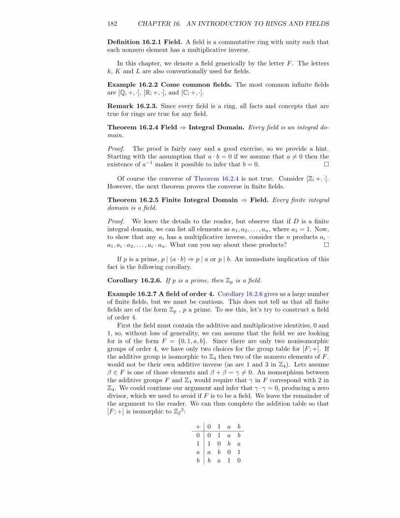
182 CHAPTER 16. AN INTRODUCTION TO RINGS AND FIELDS
Definition 16.2.1 Field. A field is a commutative ring with unity such thateach nonzero element has a multiplicative inverse.
In this chapter, we denote a field generically by the letter F . The lettersk, K and L are also conventionally used for fields.
Example 16.2.2 Come common fields. The most common infinite fieldsare [Q,+, ·], [R; +, ·], and [C; +, ·].
Remark 16.2.3. Since every field is a ring, all facts and concepts that aretrue for rings are true for any field.
Theorem 16.2.4 Field ⇒ Integral Domain. Every field is an integral do-main.
Proof. The proof is fairly easy and a good exercise, so we provide a hint.Starting with the assumption that a · b = 0 if we assume that a 6= 0 then theexistence of a−1 makes it possible to infer that b = 0.
Of course the converse of Theorem 16.2.4 is not true. Consider [Z; +, ·].However, the next theorem proves the converse in finite fields.
Theorem 16.2.5 Finite Integral Domain ⇒ Field. Every finite integraldomain is a field.
Proof. We leave the details to the reader, but observe that if D is a finiteintegral domain, we can list all elements as a1, a2, . . . , an, where a1 = 1. Now,to show that any ai has a multiplicative inverse, consider the n products ai ·a1, ai · a2, . . . , ai · an. What can you say about these products?
If p is a prime, p | (a · b)⇒ p | a or p | b. An immediate implication of thisfact is the following corollary.
Corollary 16.2.6. If p is a prime, then Zp is a field.
Example 16.2.7 A field of order 4. Corollary 16.2.6 gives us a large numberof finite fields, but we must be cautious. This does not tell us that all finitefields are of the form Zp , p a prime. To see this, let’s try to construct a fieldof order 4.
First the field must contain the additive and multiplicative identities, 0 and1, so, without loss of generality, we can assume that the field we are lookingfor is of the form F = {0, 1, a, b}. Since there are only two nonisomorphicgroups of order 4, we have only two choices for the group table for [F ; +]. Ifthe additive group is isomorphic to Z4 then two of the nonzero elements of F .would not be their own additive inverse (as are 1 and 3 in Z4). Lets assumeβ ∈ F is one of those elements and β + β = γ 6= 0. An isomorphism betweenthe additive groups F and Z4 would require that γ in F correspond with 2 inZ4. We could continue our argument and infer that γ ·γ = 0, producing a zerodivisor, which we need to avoid if F is to be a field. We leave the remainder ofthe argument to the reader. We can thus complete the addition table so that[F ; +] is isomorphic to Z2
2:
+ 0 1 a b
0 0 1 a b
1 1 0 b a
a a b 0 1
b b a 1 0
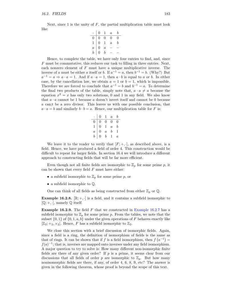
16.2. FIELDS 183
Next, since 1 is the unity of F , the partial multiplication table must looklike:
· 0 1 a b
0 0 0 0 0
1 0 1 a b
a 0 a − −b 0 b − −
Hence, to complete the table, we have only four entries to find, and, sinceF must be commutative, this reduces our task to filling in three entries. Next,each nonzero element of F must have a unique multiplicative inverse. Theinverse of a must be either a itself or b. If a−1 = a, then b−1 = b. (Why?) Buta−1 = a ⇒ a · a = 1. And if a · a = 1, then a · b is equal to a or b. In eithercase, by the cancellation law, we obtain a = 1 or b = 1, which is impossible.Therefore we are forced to conclude that a−1 = b and b−1 = a. To determinethe final two products of the table, simply note that, a · a 6= a because theequation x2 = x has only two solutions, 0 and 1 in any field. We also knowthat a · a cannot be 1 because a doesn’t invert itself and cannot be 0 becausea can;t be a zero divisor. This leaves us with one possible conclusion, thata · a = b and similarly b · b = a. Hence, our multiplication table for F is:
· 0 1 a b
0 0 0 0 0
1 0 1 a b
a 0 a b 1
b 0 b 1 a
We leave it to the reader to verify that [F ; +, ·], as described above, is afield. Hence, we have produced a field of order 4. This construction would bedifficult to repeat for larger fields. In section 16.4 we will introduce a differentapproach to constructing fields that will be far more efficient.
Even though not all finite fields are isomorphic to Zp for some prime p, itcan be shown that every field F must have either:
• a subfield isomorphic to Zp for some prime p, or
• a subfield isomorphic to Q.
One can think of all fields as being constructed from either Zp or Q.
Example 16.2.8. [R; +, ·] is a field, and it contains a subfield isomorphic to[Q; +, ·], namely Q itself.
Example 16.2.9. The field F that we constructed in Example 16.2.7 has asubfield isomorphic to Zp for some prime p. From the tables, we note that thesubset {0, 1} of {0, 1, a, b} under the given operations of F behaves exactly like[Z2; +2,×2]. Hence, F has a subfield isomorphic to Z2.
We close this section with a brief discussion of isomorphic fields. Again,since a field is a ring, the definition of isomorphism of fields is the same asthat of rings. It can be shown that if f is a field isomorphism, then f
(a−1
)=
f(a)−1; that is, inverses are mapped onto inverses under any field isomorphism.A major question to try to solve is: How many different non-isomorphic finitefields are there of any given order? If p is a prime, it seems clear from ourdiscussions that all fields of order p are isomorphic to Zp. But how manynonisomorphic fields are there, if any, of order 4, 6, 8, 9, etc? The answer isgiven in the following theorem, whose proof is beyond the scope of this text.
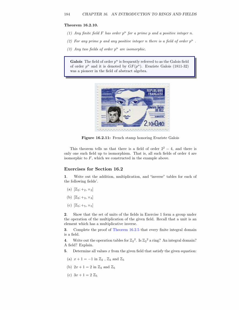
184 CHAPTER 16. AN INTRODUCTION TO RINGS AND FIELDS
Theorem 16.2.10.
(1) Any finite field F has order pn for a prime p and a positive integer n.
(2) For any prime p and any positive integer n there is a field of order pn .
(3) Any two fields of order pn are isomorphic.
Galois The field of order pn is frequently referred to as the Galois fieldof order pn and it is denoted by GF (pn). Evariste Galois (1811-32)was a pioneer in the field of abstract algebra.
Figure 16.2.11: French stamp honoring Evariste Galois
This theorem tells us that there is a field of order 22 = 4, and there isonly one such field up to isomorphism. That is, all such fields of order 4 areisomorphic to F , which we constructed in the example above.
Exercises for Section 16.2
1. Write out the addition, multiplication, and “inverse” tables for each ofthe following fields’.
(a) [Z2; +2,×2]
(b) [Z3; +3,×3]
(c) [Z5; +5,×5]
2. Show that the set of units of the fields in Exercise 1 form a group underthe operation of the multiplication of the given field. Recall that a unit is anelement which has a multiplicative inverse.3. Complete the proof of Theorem 16.2.5 that every finite integral domainis a field.4. Write out the operation tables for Z2
2. Is Z22 a ring? An integral domain?
A field? Explain.5. Determine all values x from the given field that satisfy the given equation:
(a) x+ 1 = −1 in Z2 , Z3 and Z5
(b) 2x+ 1 = 2 in Z3 and Z5
(c) 3x+ 1 = 2 Z5
16.3. POLYNOMIAL RINGS 185
6.
(a) Prove that if p and q are prime, then Zp × Zq, is never a field.
(b) Can Zpn be a field for any prime p and any positive integer n ≥ 2?
7. Determine all solutions to the following equations over Z2. That is, findall elements of Z2 that satisfy the equations.
(a) x2 + x = 0
(b) x2 + 1 = 0
(c) x3 + x2 + x+ 1 = 0
(d) x3 + x+ 1 = 0
8. Determine the number of different fields, if any, of all orders 2 through15. Wherever possible, describe these fields via a known field.9. Let Q
(√2)
={a+ b
√2∣∣ a, b ∈ Q}.
(a) Prove that[Q(√
2)
; +, ·]is a field.
(b) Show that Q is a subfield of Q(√
2). For this reason, Q
(√2)is called
an extension field of Q.
(c) Show that all the roots of the equation x2−4x+ 72 = 0 lie in the extension
field Q(√
2).
(d) Do the roots of the equation x2 − 4x+ 3 = 0 lie in this field? Explain.
16.3 Polynomial Rings
In the previous sections we examined the solutions of a few equations overdifferent rings and fields. To solve the equation x2 − 2 = 0 over the field ofthe real numbers means to find all solutions of this equation that are in thisparticular field R. This statement can be replaced as follows: Determine alla ∈ R such that the polynomial f(x) = x2 − 2 is equal to zero when evaluatedat x = a. In this section, we will concentrate on the theory of polynomials.We will develop concepts using the general setting of polynomials over ringssince results proven over rings are true for fields (and integral domains). Thereader should keep in mind that in most cases we are just formalizing conceptsthat he or she learned in high school algebra over the field of reals.
Definition 16.3.1 Polynomial over a Ring. Let [R; +, ·] be a ring. Apolynomial, f(x), over R is an expression of the form
f(x) =
n∑i=0
aixi = a0 + a1x+ a2x
2 + · · ·+ anxn
where n ≥ 0, and a0, a1, a2, . . . , an ∈ R. If an 6= 0, then the degree of f(x) isn, If f(x) = 0, then the degree of f(x) is undefined, but for convience we saythat deg 0 = −∞. If the degree of f(x) is n, we write deg f(x) = n. The setof all polynomials in the indeterminate x with coefficients in R is denoted byR[x].
Note 16.3.2.
186 CHAPTER 16. AN INTRODUCTION TO RINGS AND FIELDS
• The symbol x is an object called an indeterminate, which is not anelement of the ring R.
• Note that R ⊆ R[x], The elements of R are called constant polynomials,with the nonzero elements of R being the polynomials of degree 0.
• R is called the ground, or base, ring for R[x].
• In the definition above, we have written the terms in increasing degreestarting with the constant. The ordering of terms can be reversed withoutchanging the polynomial. For example, 1 + 2x− 3x4 and −3x4 + 2x+ 1are the same polynomial.
• A term of the form xk in a polynomial is understood to be 1xk.
• It is understood that if deg f(x) = n, then coefficients of powers of xhigher than n are equal to the zero of the base ring.
Definition 16.3.3 Polynomial Addition. Let f(x) = a0 + a1x + a2x2 +
· · · + amxm and g(x) = b0 + b1x + b2x
2 + · · · + bnxn be elements in R[x] so
that ai ∈ R and bi ∈ R for all i. Let k be the maximum of m and n. Thenf(x)+g(x) = c0+c1x+c2x
2+· · ·+ckxk, where ci = ai+bi for i = 0, 1, 2, . . . , k.
Definition 16.3.4 Polynomial Multiplication. Let f(x) = a0 + a1x +a2x
2 + · · ·+ amxm and g(x) = b0 + b1x+ b2x
2 + · · ·+ bnxn. Then
f(x) · g(x) = d0 + d1x+ d2x2 + · · ·+ dpx
p where p = m+ n andds =
∑si=0 aibs−i = a0bs + a1bs−1 + a2bs−2 + · · ·+ as−1b1 + asb0
for 0 ≤ s ≤ p
The important fact to keep in mind is that addition and multiplicationin R[x] depends on addition and multiplication in R. The powers of x merelyserve the purpose of “place holders.” All computations involving coefficients aredone over the given ring. Powers of the indeterminate are computed formallyapplying the rule of adding exponents when multiplying powers.
Example 16.3.5. f(x) = 3, g(x) = 2 − 4x + 7x2 , and h(x) = 2 + x4 are allpolynomials in Z[x]. Their degrees are 0, 2, and 4, respectively.
Addition and multiplication of polynomials are performed as in high schoolalgebra. However, we must do our computations in the ground ring of thepolynomials.
Example 16.3.6. In Z3[x], if f(x) = 1 + x and g(x) = 2 + x, then
f(x) + g(x) = (1 + x) + (2 + x)
= (1 +3 2) + (1 +3 1)x
= 0 + 2x
= 2x
and
f(x)g(x) = (1 + x) · (2 + x)
= 1×3 2 + (1×3 1 +3 1×3 2)x2 + (1×3 2)x2
= 2 + 0x+ x2
= 2 + x2
16.3. POLYNOMIAL RINGS 187
However, for the same polynomials as above, f(x) and g(x) in the more familiarsetting of Z[x], we have
f(x) + g(x) = (1 + x) + (2 + x) = (1 + 2) + (1 + 1)x = 3 + 2x
and
f(x)g(x) = (1 + x) · (2 + x)
= 1 · 2 + (1 · 1 + 1 · 2)x+ (1 · 1)x2
= 2 + 3x+ x2
Example 16.3.7. Let f(x) = 2 + x2 and g(x) = −1 + 4x + 3x2. We willcompute f(x) · g(x) in Z[x]. Of course this product can be obtained by theusual methods of high school algebra. We will, for illustrative purposes, use theabove definition. Using the notation of the above definition, a0 = 2, a1 = 0,a2 = 1, b0 = −1, b1 = 4, and b2 = 3. We want to compute the coefficients d0,d1, d2, d3, and d4 . We will compute d3 , the coefficient of the x3 term of theproduct, and leave the remainder to the reader (see Exercise 2 of this section).Since the degrees of both factors is 2, ai = bi = 0 for i ≥ 3. The coefficient ofx3 is
d3 = a0b3 + a1b2 + a2b1 + a3b0 = 2 · 0 + 0 · 3 + 1 · 4 + 0 · (−1) = 4
The proofs of the following theorem are not difficult but rather long, so weomit them.
Theorem 16.3.8 Properties of Polynomial Rings. Let [R; +, ·] be a ring.Then:
(1) R[x] is a ring under the operations of polynomial addition and multipli-cation.
(2) If R is a commutative ring, then R[x] is a commutative ring.
(3) If R is a ring with unity, 1, then R[x] is a ring with unity (the unity inR[x] is 1 + 0x+ 0x2 + · · ·).
(4) If R is an integral domain, then R[x] is an integral domain.
(5) If F is a field, then F [x] is not a field. However, F [x] is an integraldomain.
Next we turn to division of polynomials, which is not an operation since theresult is a pair of polynomials, not a single one. From high school algebra weall learned the standard procedure for dividing a polynomial f(x) by a secondpolynomial g(x). This process of polynomial long division is referred to as thedivision property for polynomials. Under this scheme we continue to divideuntil the result is a quotient q(x) and a remainder r(x) whose degree is strictlyless than that of the divisor g(x). This property is valid over any field. Beforegiving a formal description, we consider some examples.
Example 16.3.9 Polynomial Division. Let f(x) = 1 + x+ x3 and g(x) =1 + x be two polynomials in Z2[x]. Let us divide f(x) by g(x). Keep in mindthat we are in Z2[x] and that, in particular, −1 = 1 in Z2 . This is a casewhere reordering the terms in decreasing degree is preferred.
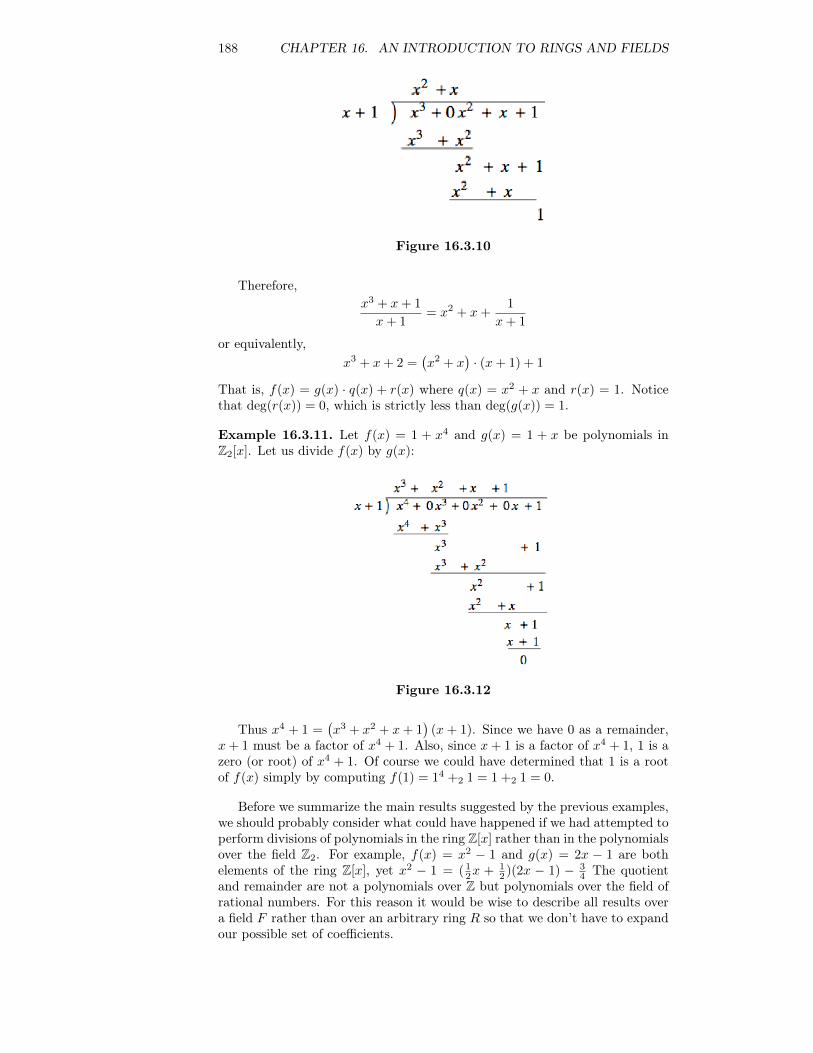
188 CHAPTER 16. AN INTRODUCTION TO RINGS AND FIELDS
Figure 16.3.10
Therefore,x3 + x+ 1
x+ 1= x2 + x+
1
x+ 1
or equivalently,x3 + x+ 2 =
(x2 + x
)· (x+ 1) + 1
That is, f(x) = g(x) · q(x) + r(x) where q(x) = x2 + x and r(x) = 1. Noticethat deg(r(x)) = 0, which is strictly less than deg(g(x)) = 1.
Example 16.3.11. Let f(x) = 1 + x4 and g(x) = 1 + x be polynomials inZ2[x]. Let us divide f(x) by g(x):
Figure 16.3.12
Thus x4 + 1 =(x3 + x2 + x+ 1
)(x + 1). Since we have 0 as a remainder,
x+ 1 must be a factor of x4 + 1. Also, since x+ 1 is a factor of x4 + 1, 1 is azero (or root) of x4 + 1. Of course we could have determined that 1 is a rootof f(x) simply by computing f(1) = 14 +2 1 = 1 +2 1 = 0.
Before we summarize the main results suggested by the previous examples,we should probably consider what could have happened if we had attempted toperform divisions of polynomials in the ring Z[x] rather than in the polynomialsover the field Z2. For example, f(x) = x2 − 1 and g(x) = 2x − 1 are bothelements of the ring Z[x], yet x2 − 1 = ( 1
2x + 12 )(2x − 1) − 3
4 The quotientand remainder are not a polynomials over Z but polynomials over the field ofrational numbers. For this reason it would be wise to describe all results overa field F rather than over an arbitrary ring R so that we don’t have to expandour possible set of coefficients.
16.3. POLYNOMIAL RINGS 189
Theorem 16.3.13 Division Property for Polynomials. Let [F ; +, ·] be afield and let f(x) and g(x) be two elements of F [x] with g(x) 6= 0. Then thereexist unique polynomials q(x) and r(x) in F [x] such that f(x) = g(x)q(x)+r(x),where deg r(x) < deg g(x).
Proof. This theorem can be proven by induction on deg f(x).
Theorem 16.3.14 The Factor Theorem. Let [F ; +, ·] be a field. An elementa ∈ F is a zero of f(x) ∈ F [x] if and only if x− a is a factor of f(x) in F [x].
Proof. (⇒) Assume that a ∈ F is a zero of f(x) ∈ F [x]. We wish to showthat x − a is a factor of f(x). To do so, apply the division property to f(x)and g(x) = x − a. Hence, there exist unique polynomials q(x) and r(x) fromF [x] such that f(x) = (x− a) · q(x) + r(x) and the deg r(x) < deg(x− a) = 1,so r(x) = c ∈ F , that is, r(x) is a constant. Also, the fact that a is a zeroof f(x) means that f(a) = 0. So f(x) = (x − a) · q(x) + c becomes 0 =f(a) = (a − a)q(a) + c. Hence c = 0, so f(x) = (x − a) · q(x), and x − a isa factor of f(x). The reader should note that a critical point of the proof ofthis half of the theorem was the part of the division property that stated thatdeg r(x) < deg g(x).
(⇐) We leave this half to the reader as an exercise.
Theorem 16.3.15. A nonzero polynomial f(x) ∈ F [x] of degree n can haveat most n zeros.
Proof. Let a ∈ F be a zero of f(x). Then f(x) = (x−a) · q1(x), q1(x) ∈ F [x],by the Factor Theorem. If b ∈ F is a zero of q1(x), then again by FactorTheorem, f(x) = (x − a)(x − b)q2(x), q2(x) ∈ F [x]. Continue this process,which must terminate in at most n steps since the degree of qk(x) would ben− k.
From The Factor Theorem, we can get yet another insight into the problemsassociated with solving polynomial equations; that is, finding the zeros of apolynomial. The initial important idea here is that the zero a is from theground field F . Second, a is a zero only if (x − a) is a factor of f(x) in F [x];that is, only when f(x) can be factored (or reduced) to the product of (x− a)times some other polynomial in F [x].
Example 16.3.16. Consider the polynomial f(x) = x2 − 2 taken as being inQ[x]. From high school algebra we know that f(x) has two zeros (or roots),namely ±
√2, and x2 − 2 can be factored as
(x−√
2) (x+√
2). However, we
are working in Q[x], these two factors are not in the set of polynomials overthe rational numbers, Q since
√2 /∈ Q . Therefore, x2− 2 does not have a zero
in Q since it cannot be factored over Q. When this happens, we say that thepolynomial is irreducible over Q.
The problem of factoring polynomials is tied hand-in-hand with that of thereducibility of polynomials. We give a precise definition of this concept.
Definition 16.3.17 Reducibility over a Field. Let [F ; +, ·] be a field andlet f(x) ∈ F [x] be a nonconstant polynomial. f(x) is reducible over F if andonly if it cannot be factored as a product of two nonconstant polynomials inF [x]. A polynomial is irreducible over F if it is not reducible over F .
Example 16.3.18. The polynomial f(x) = x4 + 1 is reducible over Z2 sincex4 + 1 = (x+ 1)
(x3 + x2 + x− 1
).
190 CHAPTER 16. AN INTRODUCTION TO RINGS AND FIELDS
Example 16.3.19. Is the polynomial f(x) = x3 + x + 1 reducible over Z2?Since a factorization of a cubic polynomial can only be as a product of linearand quadratic factors, or as a product of three linear factors, f(x) is reducibleif and only if it has at least one linear factor. From the Factor Theorem, x− ais a factor of x3 +x+ 1 over Z2 if and only if a ∈ Z2 is a zero of x3 +x+ 1. Sox3 + x+ 1 is reducible over Z2 if and only if it has a zero in Z2 . Since Z2 hasonly two elements, 0 and 1, this is easy enough to check. f(0) = 03+20+21 = 1and f(1) = 13 +2 1+2 1 = 1, so neither 0 nor 1 is a zero of f(x) over Z2. Hence,x3 + x+ 1 is irreducible over Z2.
From high school algebra we know that x3 + x + 1 has three zeros fromsome field. Can we find this field? To be more precise, can we construct thefield that contains Z2 and all zeros of x3 +x+ 1? We will consider this task inthe next section.
We close this section with a final analogy. Prime numbers play an importantrole in mathematics. The concept of irreducible polynomials (over a field) isanalogous to that of a prime number. Just think of the definition of a primenumber. A useful fact concerning primes is: If p is a prime and if p | ab, thenp | a or p | b. We leave it to the reader to think about the veracity of thefollowing: If p(x) is an irreducible polynomial over F , a(x), b(x) ∈ F [x] andp(x) | a(x)b(x), then p(x) | a(x) or p(x) | b(x).
Exercises for Section 16.31. Let f(x) = 1 + x and g(x) = 1 + x + x2. Compute the following sumsand products in the indicated rings.
(a) f(x) + g(x) and f(x) · g(x) in Z[x]
(b) f(x) + g(x) and f(x) · g(x) in Z2[x]
(c) (f(x) · g(x)) · f(x) in Q[x]
(d) (f(x) · g(x)) · f(x) in Z2[x]
(e) f(x) · f(x) + f(x) · g(x) in Z2[x]
2. Complete the calculations started in Example 16.3.7.3. Prove that:
(a) The ring R is a subring of the ring R[x].
(b) The ring Z[x] is a subring of the Q[x].
(c) The ring Q[x] is a subring of the ring R[x].
4.
(a) Find all zeros of x4 + 1 in Z3.
(b) Find all zeros of x5 + 1 in Z5.
5. Determine which of the following are reducible over Z2. Explain.
(a) f(x) = x3 + 1
(b) g(x) = x3 + x2 + x.
(c) h(x) = x3 + x2 + 1.
16.4. FIELD EXTENSIONS 191
(d) k(x) = x4 + x2 + 1. (Be careful.)
6. Prove the second half of The Factor Theorem.
7. Give an example of the contention made in the last paragraph of thissection.
8. Determine all zeros of x4 + 3x3 + 2x+ 4 in Z5[x]
9. Show that x2 − 3 is irreducible over Q but reducible over the field of realnumbers.
10. The definition of a vector space given in Chapter 13 holds over any fieldF , not just over the field of real numbers, where the elements of F are calledscalars.
(a) Show that F [x] is a vector space over F .
(b) Find a basis for F [x] over F .
(c) What is the dimension of F [x] over F?
11. Prove Theorem 16.3.13, the Division Property for Polynomials
12.
(a) Show that the field R of real numbers is a vector space over R. Find abasis for this vector space. What is dim R over R?
(b) Repeat part a for an arbitrary field F.
(c) Show that R is a vector space over Q.
16.4 Field Extensions
From high school algebra we realize that to solve a polynomial equation meansto find its roots (or, equivalently, to find the zeros of the polynomials). FromExample 16.3.16 and Example 16.3.19 we know that the zeros may not liein the given ground field. Hence, to solve a polynomial really involves twosteps: first, find the zeros, and second, find the field in which the zeros lie. Foreconomy’s sake we would like this field to be the smallest field that contains allthe zeros of the given polynomial. To illustrate this concept, let us reconsiderthe examples from the previous section..
Example 16.4.1 Extending the Rational Numbers. Let f(x) = x2−2 ∈Q[x]. It is important to remember that we are considering x2 − 2 over Q, noother field. We would like to find all zeros of f(x) and the smallest field, callit S for now, that contains them. The zeros are x = ±
√2, neither of which is
an element of Q. The set S we are looking for must satisfy the conditions:
(1) S must be a field.
(2) S must contain Q as a subfield,
(3) S must contain all zeros of f(x) = x2 − 2
192 CHAPTER 16. AN INTRODUCTION TO RINGS AND FIELDS
By the last condition√
2 must be an element of S, and, if S is to be afield, the sum, product, difference, and quotient of elements in S must be inS. So operations involving this number, such as
√2,(√
2)2,(√
2)3,√
2 +√
2,√2 −√
2, and 1√2must all be elements of S. Further, since S contains Q as
a subset, any element of Q combined with√
2 under any field operation mustbe an element of S. Hence, every element of the form a+ b
√2, where a and b
can be any elements in Q, is an element of S. We leave to the reader to showthat S = {a + b
√2 | a, b ∈ Q} is a field (see Exercise 1 of this section). We
note that the second zero of x2 − 2, namely −√
2, is an element of this set.To see this, simply take a = 0 and b = −1. The field S is frequently denotedas Q
(√2), and it is referred to as an extension field of Q. Note that the
polynomial x2 − 2 =(x−√
2) (x+√
2)factors into linear factors, or splits,
in Q(√
2)
[x]; that is, all coefficients of both factors are elements of the fieldQ(√
2).
Example 16.4.2 Extending Z2. Consider the polynomial g(x) = x2+x+1 ∈Z2[x]. Let’s repeat the steps from the previous example to factor g(x). First,g(0) = 1 and g(1) = 1, so none of the elements of Z2 are zeros of g(x). Hence,the zeros of g(x) must lie in an extension field of Z2. By Theorem 16.3.15,g(x) = x2 + x + 1 can have at most two zeros. Let a be a zero of g(x). Thenthe extension field S of Z2 must contain, besides a, a · a = a2, a3, a + a,a+ 1, and so on. But, since g(a) = 0, we have a2 + a+ 1 = 0, or equivalently,a2 = −(a+1) = a+1 (remember, we are working in an extension of Z2). We canuse this recurrence relation to reduce powers of a. So far our extension field, S,of Z2 must contain the set {0, 1, a, a+ 1}, and we claim that this the completeextension. For S to be a field, all possible sums, products, and differences ofelements in S must be in S. Let’s try a few: a+ a = a (1 +2 1) = a · 0 = 0 ∈ SSince a+ a = 0, −a = a, which is in S. Adding three a’s together doesn’t giveus anything new: a+ a+ a = a ∈ S In fact, na is in S for all possible positiveintegers n. Next,
a3 = a2 · a= (a+ 1) · a= a2 + a
= (a+ 1) + a
= 1
Therefore, a−1 = a+ 1 = a2 and (a+ 1)−1 = a.It is not difficult to see that an is in S for all positive n. Does S contain
all zeros of x2 + x + 1? Remember, g(x) can have at most two distinct zerosand we called one of them a, so if there is a second, it must be a + 1. To seeif a+ 1 is indeed a zero of g(x), simply compute f(a+ 1):
f(a+ 1) = (a+ 1)2 + (a+ 1) + 1
= a2 + 1 + a+ 1 + 1
= a2 + a+ 1
= 0
Therefore, a + 1 is also a zero of x2 + x + 1. Hence, S = {0, 1, a, a + 1} isthe smallest field that contains Z2 = {0, 1} as a subfield and contains all zerosof x2 + x+ 1. This extension field is denoted by Z2(a). Note that x2 + x+ 1splits in Z2(a); that is, it factors into linear factors in Z2(a). We also observe
16.4. FIELD EXTENSIONS 193
that Z2(a) is a field containing exactly four elements. By Theorem 16.2.10,we expected that Z2(a) would be of order p2 for some prime p and positiveinteger n. Also recall that all fields of order pn are isomorphic. Hence, wehave described all fields of order 22 = 4 by finding the extension field of apolynomial that is irreducible over Z2.
The reader might feel somewhat uncomfortable with the results obtainedin Example 16.4.2. In particular, what is a? Can we describe it through aknown quantity? All we know about a is that it is a zero of g(x) and thata2 = a+ 1. We could also say that a(a+ 1) = 1, but we really expected more.However, should we expect more? In Example 16.4.1,
√2 is a number we are
more comfortable with, but all we really know about it is that α =√
2 is thenumber such that α2 = 2. Similarly, the zero that the reader will obtain inExercise 2 of this section is the imaginary number i. Here again, this is simplya symbol, and all we know about it is that i2 = −1. Hence, the result obtainedin Example 16.4.2 is not really that strange.
The reader should be aware that we have just scratched the surface in thedevelopment of topics in polynomial rings. One area of significant applicationsis in coding theory.
Example 16.4.3 An Error Correcting Polynomial Code. An importantobservation regarding the previous example is that the nonzero elements ofGF (4) can be represented two ways. First as a linear combination of 1 anda. There are four such linear combinations, one of which is zero. Second, aspowers of a. There are three distinct powers and the each match up with anonzero linear combination:
a0 = 1 · 1 + 0 · aa1 = 0 · 1 + 1 · aa2 = 1 · 1 + 1 · a
Next, we briefly describe the field GF (8) and how an error correcting codecan be build on a the same observation about that field.
First, we start with the irreducible polynomial p(x) = x3 + x+ 1 over Z2.There is another such cubic polynomial, but its choice produces essentially thesame result. Just as we did in the previous example, we assume we have a zeroof p(x) and call it β. Since we have assumed that p(β) = β3 + β + 1 = 0, weget the recurrence relation for powers β3 = β + 1 that lets us reduce the sevenpowers βk, 0 ≤ k ≤ 6, to linear combinations of 1, β, and β2. Higher powerswill reduce to these seven, which make up the elements of a field with 23 = 8elements when we add zero to the set. We leave as an exercise for you to setup a table relating powers of β with the linear combinations.
With this information we are now in a position to take blocks of four bitsand encode them with three parity bits to create an error correcting code. If thebits are b3b4b5b6, then we reduce the expression Bm = b3 ·β3+b4 ·β4+b5 ·β5+b6 ·β6 using the recurrence relation to an expression Bp = b0 ·1+b1 ·β+b2 ·β2. Sincewe are equating equals within GF (8), we have Bp = Bm, or Bp+Bm = 0. Theencoded message is b0b1b2b3b4b5b6, which is a representation of 0 in GF (8).If the transmitted sequence of bits is received as c0c1c2c3c4c5c6 we reduceC = c0 ·1+c1 ·β+c2 ·β2 +c3 ·β3 +c4 ·β4 +c5 ·β5 +c6 ·β6 using the recurrence.If there was no transmission error, the result is zero. If the reduced result iszero it is most likely that the original message was c3c4c5c6. If bit k is switchedin the transmission, then
C = Bp +Bm + βk = βk
194 CHAPTER 16. AN INTRODUCTION TO RINGS AND FIELDS
Therefore if we reduce C with the recurrence, we get the linear combinationof 1, β, and β2 that is equal to βk and so we can identify the location of theerror and correct it.
Exercises for Section 16.41.
(a) Use the definition of a field to show that Q(√
2) is a field.
(b) Use the definition of vector space to show that Q(√
2)is a vector space
over Q.
(c) Prove that{
1,√
2}is a basis for the vector space Q
(√2)over Q, and,
therefore, the dimension of Q(√
2) over Q is 2.
2.
(a) Determine the splitting field of f(x) = x2+1 over R. This means considerthe polynomial f(x) = x2 + 1 ∈ R[x] and find the smallest field thatcontains R and all the zeros of f(x). Denote this field by R(i).
(b) R(i) is more commonly referred to by a different name. What is it?
(c) Show that {1, i} is a basis for the vector space R(i) over R. What is thedimension of this vector space (over R)?
3. Determine the splitting field of x4 − 5x2 + 6 over Q.4.
(a) Factor x2 + x+ 1 into linear factors in Z2(a).
(b) Write out the field tables for the field Z2(a) and compare the results tothe tables of Example 16.2.7.
(c) Cite a theorem and use it to show why the results of part b were to beexpected.
5.
(a) Show that x3 + x+ 1 is irreducible over Z2.
(b) Determine the splitting field of x3 + x+ 1 over Z2.
(c) By Theorem 16.2.10, you have described all fields of order 23.
6.
(a) List all polynomials of degree 1, 2, 3, and 4 over Z2 = GF (2).
(b) From your list in part a, identify all irreducible polynomials of degree 1,2, 3, and 4.
(c) Determine the splitting fields of each of the polynomials in part b.
(d) What is the order of each of the splitting fields obtained in part c? Ex-plain your results using Theorem 16.2.10.
7. Is the polynomial code described in this section a linear code?
16.5. POWER SERIES 195
16.5 Power Series
16.5.1 DefinitionEarlier in this chapter, we found that a polynomial of degree n over a ring Ris an expression of the form
f(x) =
n∑i=0
aixi = a0 + a1x+ a2x
2 + · · ·+ anxn
where n ≥ 0, each of the ai are elements of R and an 6= 0. In Section 8.5 wedefined a generating function of a sequence s with terms s0, s1, s2, . . . as theinfinite sum
G(s, z) =
∞∑i=0
sizi = s0 + s1z + s2z
2 + · · ·
The main difference between these two expressions, disregarding notation,is that the latter is an infinite expression and the former is a finite expression.In this section we will extend the algebra of polynomials to the algebra ofinfinite expressions like G(s, z), which are called power series.
Definition 16.5.1 Power Series. Let [R; +, ·] be a ring. A power series overR is an expression of the form
f(x) =
∞∑i=0
aixi = a0 + a1x+ a2x
2 + · · ·
where a1, a2, a3, . . . ∈ R. The set of all such expressions is denoted by R[[x]].
Our first observation in our comparison of R[x] and R[[x]] is that everypolynomial is a power series and so R[x] ⊆ R[[x]]. This is true because apolynomial a0 +a1x+a2x
2 + · · ·+anxn of degree n in R[x], can be thought of
as an infinite expression where ai = 0 for i > n. In addition, we will see thatR[[x]] is a ring with subring R[x].
R[[x]] is given a ring structure by defining addition and multiplication onpower series as we did in R[x], with the modification that, since we are dealingwith infinite expressions, the sums and products will remain infinite expressionsthat we can determine term by term, as was done in with polynomials.
Definition 16.5.2 Power Series Addition. Given power series
f(x) =∑∞i=0 aix
i = a0 + a1x+ a2x2 + · · · and
g(x) =∑∞i=0 bix
i = b0 + b1x+ b2x2 + · · ·
their sum is
f(x) + g(x) =
∞∑i=0
(ai + bi)xi
= (a0 + a1) + (a1 + b1)x+ (a2 + b2)x2 + (a3 + b3)x3 + · · ·.
Definition 16.5.3 Power Series Multiplication. Given power series
f(x) =∑∞i=0 aix
i = a0 + a1x+ a2x2 + · · · and
g(x) =∑∞i=0 bix
i = b0 + b1x+ b2x2 + · · ·
their product is
f(x) · g(x) =
∞∑i=0
dixi where di =
i∑j=0
ajbi−j
= (a0 · b0) + (a0 · b1 + a1 · b0)x+ (a0 · b2 + a1 · b1 + a2 · b0)x2 + · · ·
.
196 CHAPTER 16. AN INTRODUCTION TO RINGS AND FIELDS
Example 16.5.4 Some Power Series Calcuations. Let
f(x) =∑∞i=0 ix
i = 0 + 1x+ 2x2 + 3x3 + · · · andg(x) =
∑∞i=0 2ixi = 1 + 2x+ 4x2 + 8x3 + · · ·
be elements in Z[[x]]. Let us compute f(x) + g(x) and f(x) · g(x). First thesum:
f(x) + g(x) =
∞∑i=0
ixi +
∞∑i=0
2ixi
=
∞∑i=0
(i+ 2i
)xi
= 1 + 3x+ 6x2 + 11x3 + · · ·
The product is a bit more involved:
f(x) · g(x) =
( ∞∑i=0
ixi
)·
( ∞∑i=0
2ixi
)=(0 + 1x+ 2x2 + 3x3 + · · ·
)·(1 + 2x+ 4x2 + 8x3 + · · ·
)= 0 · 1 + (0 · 2 + 1 · 1)x+ (0 · 4 + 1 · 2 + 2 · 1)x2 + · · ·= x+ 4x2 + 11x3 + · · ·
=
∞∑i=0
dixi where di =
i∑j=0
j2i−j
We can compute any value of di, with the amount of time/work required in-creasing as i increases.
def d(i):s=0for j in range(1,i+1):
s+=j*2^(i-j)return s
d(20)
2097130
A closed-form expression for di would be desirable. Using techniques fromChapter 8, the formula is di = 2i+1 − i− 2, which we leave it to the reader toderive. Hence, f(x) · g(x) =
∑∞i=0(2i+1 − i− 2)xi
16.5.2 Properties, UnitsWe have seen that addition and multiplication in R[[x]] is virtually identicalto that in R[x]. The following theorem parallels Theorem 16.3.8, establishingthe ring properties of R[[x]].
Theorem 16.5.5 Properties of Power Series. Let [R; +, ·] be a ring. Then:
(1) R[[x]] is a ring under the operations of power series addition and multi-plication, which depend on the operations in R.
(2) If R is a commutative ring, then R[[x]] is a commutative ring.
(3) If R is a ring with unity, 1, then R[[x]] is a ring with unity (the unityin R[x] is 1 + 0x+ 0x2 + · · ·).
16.5. POWER SERIES 197
(4) If R is an integral domain, then R[[x]] is an integral domain.
(5) If F is a field, then F [[x]] is not a field. However, F [[x]] is an integraldomain.
We are most interested in the situation when the set of coefficients is afield. The theorem above indicates that when F is a field, F [[x]] is an integraldomain. A reason that F [[x]] is not a field is the same as one that we can citefor F [x], namely that x does not have multiplicative inverse in F [[x]].
With all of these similarities, one might wonder if the rings of polynomialsand power series over a field are isomorphic. It turns out that they are not. Thedifference between F [x] and F [[x]] become apparent when one studies whichelements are units in each. First we prove that the only units in F [x] are thenonzero constants; that is, the nonzero elements of F .
Theorem 16.5.6 Polynomial Units. Let [F ; +, ·] be a field. Polynomialf(x) is a unit in F [x] if and only if it is a nonzero constant polynomial.
Proof. (⇒) Let f(x) be a unit in F [x]. Then f(x) has a multiplicative inverse,call it g(x), such that f(x) ·g(x) = 1. Hence, the deg(f(x) ·g(x)) = deg(1) = 0.But deg(f(x) · g(x)) = deg f(x) + deg g(x). So deg f(x) + deg g(x) = 0, andsince the degree of a polynomial is always nonnegative, this can only happenwhen the deg f(x) = deg g(x) = 0. Hence, f(x) is a constant, an element of F ,which is a unit if and only if it is nonzero.
(⇐) If f(x) is a nonzero element of F , then it is a unit since F is a field. Thusit has an inverse, which is also in F [x] and so f(x) is a unit of F [x].
Before we proceed to categorize the units in F [[x]], we remind the readerthat two power series a0 + a1x+ a2x
2 + · · · and b0 + b1x+ b2x2 + · · · are equal
if and only if corresponding coefficients are equal, ai = bi for all i ≥ 0.
Theorem 16.5.7 Power Series Units. Let [F ; +, ·] be a field. Then f(x) =∑∞i=0 aix
i is a unit of F [[x]] if and only if a0 6= 0.
Proof. (⇒) If f(x) is a unit of F [[x]], then there exists g(x) =∑∞i=0 bix
i inF [[x]] such that
f(x) · g(x) =(a0 + a1x+ a2x
2 + · · ·)·(b0 + b1x+ b2x
2 + · · ·)
= 1
= 1 + 0x+ 0x2 + · · ·.
Since corresponding coefficients in the equation above must be equal, a0 ·b0 = 1, which implies that a0 6= 0.
(⇐) Assume that a0 6= 0. To prove that f(x) is a unit of F [[x]] we need tofind g(x) =
∑∞i=0 bix
i in F [[x]] such that f(x) · g(x) =∑∞i=0 dix
i = 1. If weuse the formula for the coefficients f(x) · g(x) and equate coefficients, we get
d0 = a0 · b0 = 1 ⇒ b0 = a0−1
d1 = a0 · b1 + a1 · b0 = 0 ⇒ b1 = −a0−1 · (a1 · b0)
d2 = a0b2 + a1b1 + a2b0 = 0 ⇒ b2 = −a0−1 · (a1 · b1 + a2 · b0)
......
...ds = a0 · bs + a1 · bs−1 + · · ·+ as · b0 = 0
⇒ bs = −a0−1 · (a1 · bs−1 + a2 · bs−2 + · · ·+ as · b0)
.
Therefore the powers series∑∞i=0 bix
i is an expression whose coefficientslie in F and that satisfies the statement f(x) · g(x) = 1. Hence, g(x) is themultiplicative inverse of f(x) and f(x) is a unit.
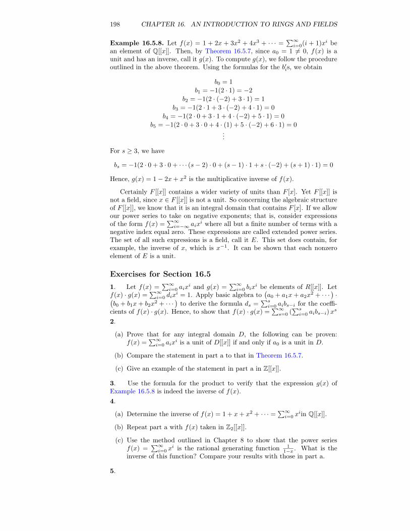
198 CHAPTER 16. AN INTRODUCTION TO RINGS AND FIELDS
Example 16.5.8. Let f(x) = 1 + 2x + 3x2 + 4x3 + · · · =∑∞i=0(i + 1)xi be
an element of Q[[x]]. Then, by Theorem 16.5.7, since a0 = 1 6= 0, f(x) is aunit and has an inverse, call it g(x). To compute g(x), we follow the procedureoutlined in the above theorem. Using the formulas for the b′is, we obtain
b0 = 1
b1 = −1(2 · 1) = −2
b2 = −1(2 · (−2) + 3 · 1) = 1
b3 = −1(2 · 1 + 3 · (−2) + 4 · 1) = 0
b4 = −1(2 · 0 + 3 · 1 + 4 · (−2) + 5 · 1) = 0
b5 = −1(2 · 0 + 3 · 0 + 4 · (1) + 5 · (−2) + 6 · 1) = 0...
For s ≥ 3, we have
bs = −1(2 · 0 + 3 · 0 + · · · (s− 2) · 0 + (s− 1) · 1 + s · (−2) + (s+ 1) · 1) = 0
Hence, g(x) = 1− 2x+ x2 is the multiplicative inverse of f(x).
Certainly F [[x]] contains a wider variety of units than F [x]. Yet F [[x]] isnot a field, since x ∈ F [[x]] is not a unit. So concerning the algebraic structureof F [[x]], we know that it is an integral domain that contains F [x]. If we allowour power series to take on negative exponents; that is, consider expressionsof the form f(x) =
∑∞i=−∞ aix
i where all but a finite number of terms with anegative index equal zero. These expressions are called extended power series.The set of all such expressions is a field, call it E. This set does contain, forexample, the inverse of x, which is x−1. It can be shown that each nonzeroelement of E is a unit.
Exercises for Section 16.51. Let f(x) =
∑∞i=0 aix
i and g(x) =∑∞i=0 bix
i be elements of R[[x]]. Letf(x) · g(x) =
∑∞i=0 dix
i = 1. Apply basic algebra to(a0 + a1x+ a2x
2 + · · ·)·(
b0 + b1x+ b2x2 + · · ·
)to derive the formula ds =
∑si=0 aibs−i for the coeffi-
cients of f(x) · g(x). Hence, to show that f(x) · g(x) =∑∞s=0 (
∑si=0 aibs−i)x
s
2.
(a) Prove that for any integral domain D, the following can be proven:f(x) =
∑∞i=0 aix
i is a unit of D[[x]] if and only if a0 is a unit in D.
(b) Compare the statement in part a to that in Theorem 16.5.7.
(c) Give an example of the statement in part a in Z[[x]].
3. Use the formula for the product to verify that the expression g(x) ofExample 16.5.8 is indeed the inverse of f(x).4.
(a) Determine the inverse of f(x) = 1 + x+ x2 + · · · =∑∞i=0 x
iin Q[[x]].
(b) Repeat part a with f(x) taken in Z2[[x]].
(c) Use the method outlined in Chapter 8 to show that the power seriesf(x) =
∑∞i=0 x
i is the rational generating function 11−x . What is the
inverse of this function? Compare your results with those in part a.
5.
16.5. POWER SERIES 199
(a) Determine the inverse of h(x) =∑∞i=0 2ixi in Q[[x]].
(b) Use the procedures in Chapter 8 to find a rational generating functionfor h(x) in part a. Find the multiplicative inverse of this function.
6. Let a(x) = 1 + 3x+ 9x2 + 27x3 + · · · =∑∞i=0 3ixi and b(x) = 1 +x+x2 +
x3 + · · · =∑∞i=0 x
i both in R[[x]].
(a) What are the first four terms (counting the constant term as the 0 th
term) of a(x) + b(x)?
(b) Find a closed form expression for a(x).
(c) What are the first four terms of a(x)b(x)?
7. Write as an extended power series:
(a)(x4 − x5
)−1
(b)(x2 − 2x3 + x4
)−1
8. Derive the closed form expression di = 2i+1 − i− 2 for the coefficients ofthe product f(x) · g(x) in Example 16.5.4.

200 CHAPTER 16. AN INTRODUCTION TO RINGS AND FIELDS
Appendix A
Algorithms
Computer programs, bicycle assembly instructions, knitting instructions, andrecipes all have several things in common. They all tell us how to do something;and the usual format is as a list of steps or instructions. In addition, they areusually prefaced with a description of the raw materials that are needed (theinput) to produce the end result (the output). We use the term algorithm todescribe such lists of instructions. We assume that the reader may be unfamil-iar with algorithms, so the first section of this appendix will introduce someof the components of the algorithms that appear in this book. Since we wouldlike our algorithms to become computer programs in many cases, the notationwill resemble a computer language such as Python or Sage; but our notationwill be slightly less formal. In some cases we will also translate the pseudocodeto Sage. Our goal will be to give mathematically correct descriptions of howto accomplish certain tasks. To this end, the second section of this appendixis an introduction to the Invariant Relation Theorem, which is a mechanismfor algorithm verification that is related to Mathematical Induction
A.1 An Introduction to Algorithms
Most of the algorithms in this book will contain a combination of three kindsof steps: the assignment step, the conditional step, and the loop.
A.1.1 Assignments
In order to assign a value to a variable, we use an assignment step, which takesthe form:
Variable = Expression to be computed
The equals sign in most languages is used for assignment but some languagesmay use variations such as := or a left pointing arrow. Logical equality, whichproduces a boolean result and would be used in conditional or looping steps,is most commonly expressed with a double-equals, ==.
An example of an assignment is k = n - 1 which tells us to subtract 1 fromthe value of n and assign that value to variable k. During the execution of analgorithm, a variable may take on only one value at a time. Another exampleof an assignment is k = k - 1. This is an instruction to subtract one from thevalue of k and then reassign that value to k.
201
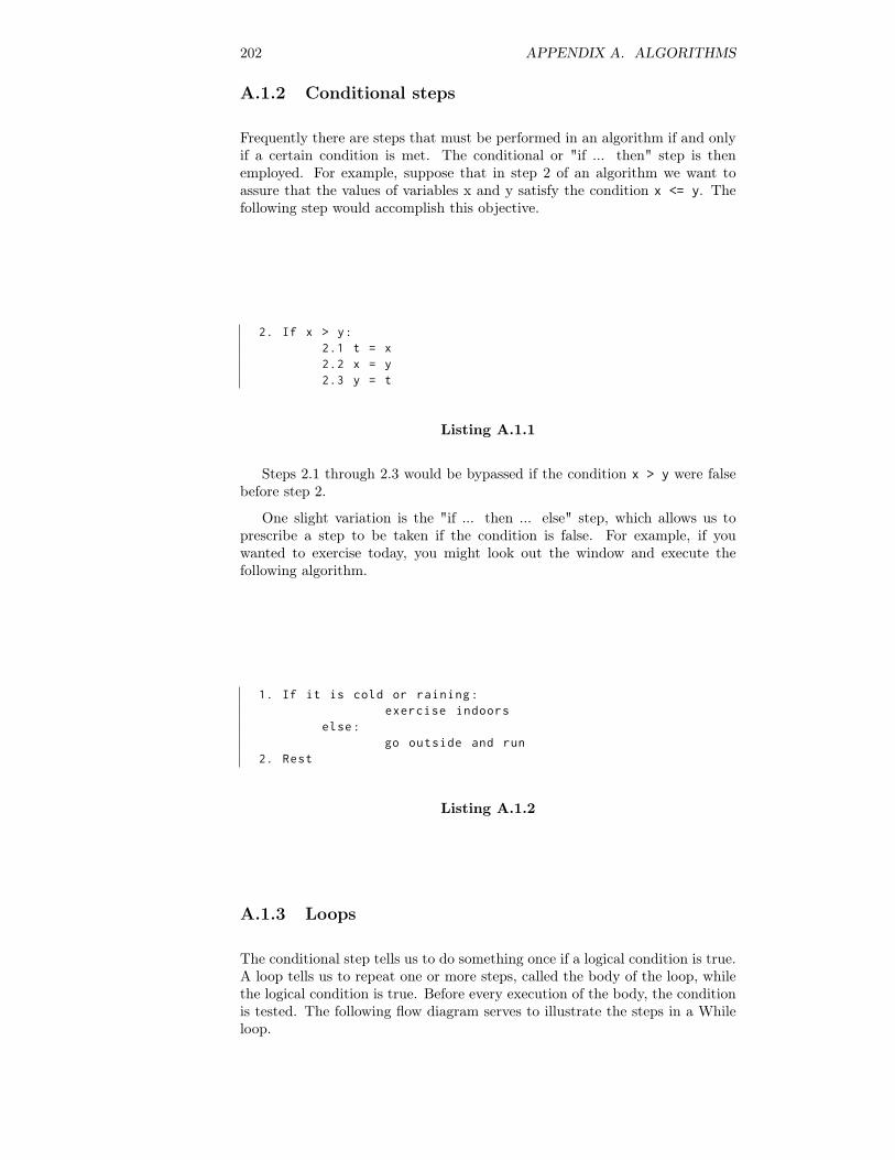
202 APPENDIX A. ALGORITHMS
A.1.2 Conditional steps
Frequently there are steps that must be performed in an algorithm if and onlyif a certain condition is met. The conditional or "if ... then" step is thenemployed. For example, suppose that in step 2 of an algorithm we want toassure that the values of variables x and y satisfy the condition x <= y. Thefollowing step would accomplish this objective.
2. If x > y:2.1 t = x2.2 x = y2.3 y = t
Listing A.1.1
Steps 2.1 through 2.3 would be bypassed if the condition x > y were falsebefore step 2.
One slight variation is the "if ... then ... else" step, which allows us toprescribe a step to be taken if the condition is false. For example, if youwanted to exercise today, you might look out the window and execute thefollowing algorithm.
1. If it is cold or raining:exercise indoors
else:go outside and run
2. Rest
Listing A.1.2
A.1.3 Loops
The conditional step tells us to do something once if a logical condition is true.A loop tells us to repeat one or more steps, called the body of the loop, whilethe logical condition is true. Before every execution of the body, the conditionis tested. The following flow diagram serves to illustrate the steps in a Whileloop.
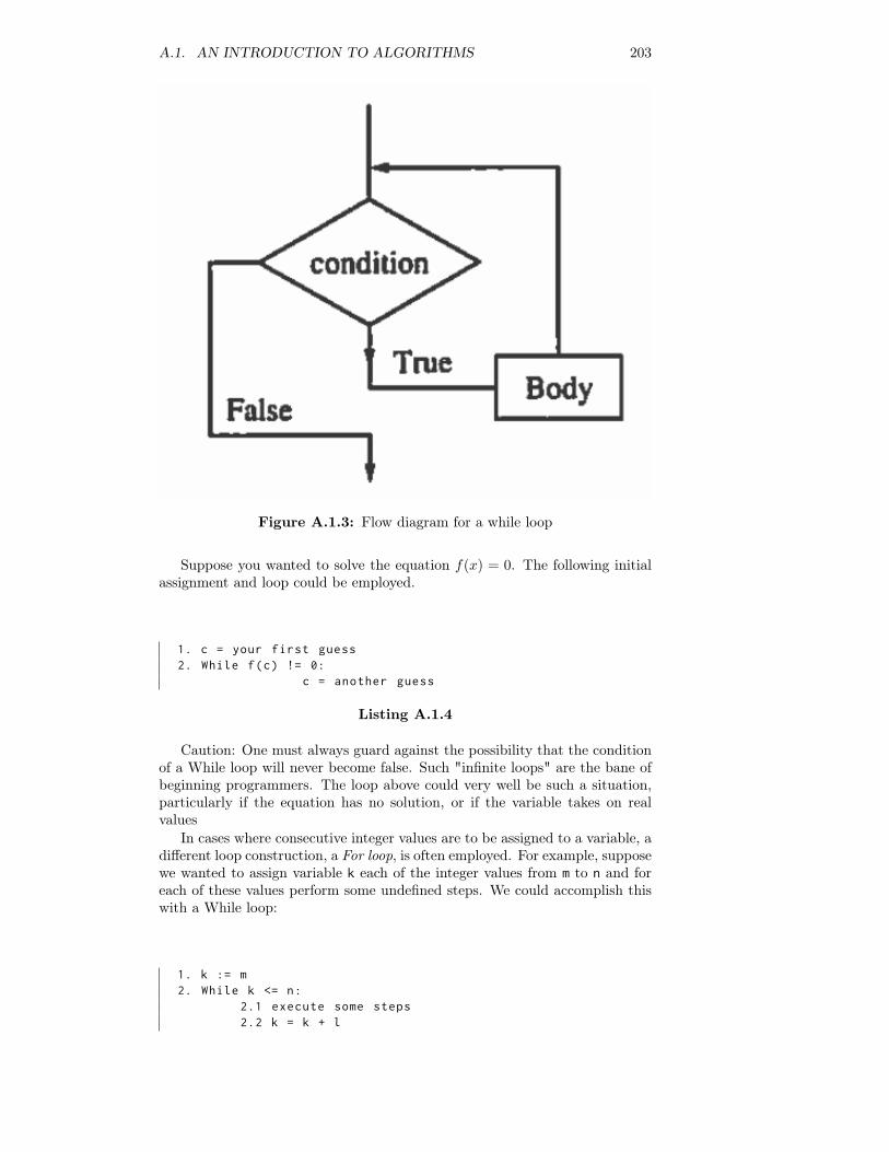
A.1. AN INTRODUCTION TO ALGORITHMS 203
Figure A.1.3: Flow diagram for a while loop
Suppose you wanted to solve the equation f(x) = 0. The following initialassignment and loop could be employed.
1. c = your first guess2. While f(c) != 0:
c = another guess
Listing A.1.4
Caution: One must always guard against the possibility that the conditionof a While loop will never become false. Such "infinite loops" are the bane ofbeginning programmers. The loop above could very well be such a situation,particularly if the equation has no solution, or if the variable takes on realvalues
In cases where consecutive integer values are to be assigned to a variable, adifferent loop construction, a For loop, is often employed. For example, supposewe wanted to assign variable k each of the integer values from m to n and foreach of these values perform some undefined steps. We could accomplish thiswith a While loop:
1. k := m2. While k <= n:
2.1 execute some steps2.2 k = k + l
204 APPENDIX A. ALGORITHMS
Listing A.1.5
Alternatively, we can perform these steps is with a For loop.
For k = m to n:execute some steps
Listing A.1.6
For loops such as this one have the advantage of being shorter than theequivalent While loop. The While loop construction has the advantage ofbeing able to handle more different situations than the For loop.
Exercises for Part 1 of the Algorithms Appendix1. What are the inputs and outputs of the algorithms listed in the firstsentence of this section?2. What is wrong with this algorithm?
Input: a and b, integersOutput: the value of c will be a - b(1) c = 0(2) While a > b:
(2.1) a := a - l(2.2) c := c + l
Listing A.1.7
3. Describe, in words, what the following algorithm does:
Input: k, a positive integerOutput: s = ?(1) s = 0(2) While k > 0:
(2.1) s = s + k(2.2) k = k - 1
Listing A.1.8
4. Write While loops to replace the For loops in the following partial algo-rithms:
(a) (1) S = 0
(2) for k = 1 to 5: S = S + k^2
(b) The floor of a number is the greatest integer less than or equal to thatnumber.
(1) m = a positive integer greater than 1
A.2. THE INVARIANT RELATION THEOREM 205
(2) B = floor(sqrt(m))
(3) for i = 2 to B: if i divides evenly into m, jump to step 5
(4) print "m is a prime" and exit
(5) print "m is composite" and exit
5. Describe in words what the following algorithm does:
Input: n, a positive integerOutput: k?(1) f= 0(2) k=n(3) While k is even:
(3.1) f = f+ 1(3.2) k = k div 2
Listing A.1.9
6. Fix the algorithm in Exercise 2.
A.2 The Invariant Relation Theorem
A.2.1 Two Exponentiation AlgorthmsConsider the following algorithm implemented in Sage to compute ammodn,given an arbitrary integer a, non-negative exponentm, and a modulus n, n ≥ 0.The default sample evaluation computes 25mod 7 = 32mod 7 = 4, but you canedit the final line for other inputs.
def slow_exp(a,m,n):b=1k=mwhile k>0:
b=(b*a)%n # % is integer remainder (mod)operation
k-=1return b
slow_exp (2,5,7)
It should be fairly clear that this algorithm will successfully compute am(modn)since it mimics the basic definition of exponentiation. However, this algorithmis highly inefficient. The algorithm that is most commonly used for the taskof exponentiation is the following one, also implemented in Sage.
def fast_exp(a,m,n):t=ab=1k=mwhile k>0:
if k%2==1: b=(b*t)%nt=(t^2)%nk=k//2 # // is the integer quotient
operation
206 APPENDIX A. ALGORITHMS
return b
fast_exp (2,5,7)
The only difficulty with the "fast algorithm" is that it might not be so obviousthat it always works. When implemented, it can be verified by example, butan even more rigorous verification can be done using the Invariant RelationTheorem. Before stating the theorem, we define some terminology.
A.2.2 Proving the correctness of the fast algorithmDefinition A.2.1 Pre and Post Values. Given a variable x, the pre valueof x, denoted x, is the value before an iteration of a loop. The post value,denoted x, is the value after the iteration.
Example A.2.2 Pre and post values in the fast exponentiation al-gorithm. In the fast exponentiation algorithm, the relationships between thepre and post values of the three variables are as follows.
b ≡ btkmod 2(modn)
t ≡ t2(modn)
k = k//2
Definition A.2.3 Invariant Relation. Given an algorithm’s inputs and aset of variables that are used in the algorithm, an invariant relation is a set ofone or more equations that are true prior to entering a loop and remain truein every iteration of the loop.
Example A.2.4 Invariant Relation for Fast Exponentiation. We claimthat the invariant relation in the fast algorithm is btk = am(modn). We willprove that his is indeed true below.
Theorem A.2.5 The Invariant Relation Theorem. Given a loop withinan algorithm, if R is a relation with the properties
(a) R is true before entering the loop
(b) the truth of R is maintained in any iteration of the loop
(c) the condition for exiting the loop will always be reached in a finite numberof iterations.
then R will be true upon exiting the loop.
Proof. The condition that the loop ends in a finite number of iterations letsus apply mathematical induction with the induction variable being the numberof iterations. We leave the details to the reader.
We can verify the correctness of the fast exponentiation algorithm usingthe Invariant Relation Theorem. First we note that prior to entering the loop,btk = 1am = am(modn). Assuming the relation is true at the start of anyiteration, that is btk = am(modn), then
btk ≡ (btk mod 2)(t2)k//2(modn)
≡ bt2(k//2)+k mod 2(modn)
≡ btk(modn)
≡ am(modn)
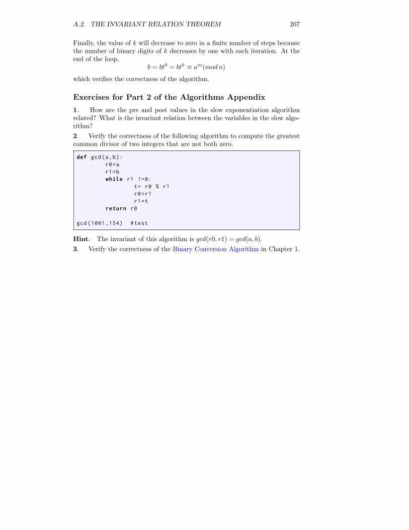
A.2. THE INVARIANT RELATION THEOREM 207
Finally, the value of k will decrease to zero in a finite number of steps becausethe number of binary digits of k decreases by one with each iteration. At theend of the loop,
b = bt0 = btk ≡ am(modn)
which verifies the correctness of the algorithm.
Exercises for Part 2 of the Algorithms Appendix1. How are the pre and post values in the slow exponentiation algorithmrelated? What is the invariant relation between the variables in the slow algo-rithm?2. Verify the correctness of the following algorithm to compute the greatestcommon divisor of two integers that are not both zero.
def gcd(a,b):r0=ar1=bwhile r1 !=0:
t= r0 % r1r0=r1r1=t
return r0
gcd (1001 ,154) #test
Hint. The invariant of this algorithm is gcd(r0, r1) = gcd(a, b).3. Verify the correctness of the Binary Conversion Algorithm in Chapter 1.

208 APPENDIX A. ALGORITHMS
Appendix B
Hints and Solutions toSelected Exercises
Exercises
7. If A and B are finite sets, how many different functions are there from Ainto B?
For each of the |A| elements of A, there are |B| possible images, so thereare|B| · |B| · . . . · |B| =
∣∣B||A| functions from A into B.
Exercises for Section 11.1
1. Determine the properties that the following operations have on the positiveintegers.
(a) addition
(b) multiplication
(c) M defined by aMb = larger ofa andb
(d) m defined by amb = smaller of a and b
(e) @ defined by a@b = ab
(a) Commutative, and associative. Notice that zero is the identity for addi-tion, but it is not a positive integer.
(b) Commutative, associative, and has an identity (1)
(c) Commutative, associative, has an identity (1), and is idempotent
(d) Commutative, associative, and idempotent
(e) None. Notice that 2@(3@3) = 512, while (2@3)@3 = 64; and a@1 = a,while 1@a = 1.
3. Let ∗ be an operation on a set S and A,B ⊆ S. Prove that if A and B areboth closed under ∗, then A∩B is also closed under ∗, but A∪B need not be.
209
210APPENDIX B. HINTS AND SOLUTIONS TO SELECTED EXERCISES
a, b ∈ A ∩B ⇒ a, b ∈ A by the definition of intersection⇒ a ∗ b inA by the closure of A with respect to ∗
Similarly, a, b ∈ A ∩ B ⇒ a ∗ b ∈ B. Therefore, a ∗ b ∈ A ∩ B. The set ofpositive integers is closed under addition, and so is the set of negative integers,but 1+−1−0. Therefore, their union, the nonzero integers, is not closed underaddition.
5. Define a ∗ b by |a− b|, the absolute value of a− b. Which properties does∗ have on the set of natural numbers, N?
(a) ∗ is commutative since |a− b| = |b− a| for all a, b ∈ N
(b) ∗ is not associative. Take a = 1, b = 2, and c = 3, then (a ∗ b) ∗ c =||1− 2| − 3| = 2 , and a ∗ (b ∗ c) = |1− |2− 3|| = 0.
(c) Zero is the identity for ∗ on N, since a ∗ 0 = |a− 0| = a = |0− a| = 0 ∗ a.
(d) Each element of N inverts itself since a ∗ a = |a− a| = 0.
(e) ∗ is not idempotent, since, for a 6= 0, a ∗ a = 0 6= a.
Exercises for Section 11.2
1. Discuss the analogy between the terms generic and concrete for algebraicsystems and the terms generic and trade for prescription drugs.
The terms “generic” and “trade” for prescription drugs are analogous to“generic” and “concrete” algebraic systems. Generic aspirin, for example, hasno name, whereas Bayer, Tylenol, Bufferin, and Anacin are all trade or specifictypes of aspirins. The same can be said of a generic group [G; ∗] where G isa nonempty set and ∗ is a binary operation on G, When examples of typicaldomain elements can be given along with descriptions of how operations act onthem, such as Q* orM2×2(R), then the system is concrete (has a specific name,as with the aspirin). Generic is a way to describe a general algebraic system,whereas a concrete system has a name or symbols making it distinguishablefrom other systems.
3. Which of the following are groups?
(a) B∗ with concatenation (see Subsection 11.2.1).
(b) M2×3(R) with matrix addition.
(c) M2×3(R) with matrix multiplication.
(d) The positive real numbers, R+,with multiplication.
(e) The nonzero real numbers, R∗, with multiplication.
(f) {1,−1} with multiplication.
(g) The positive integers with the operationM defined by aMb = the larger of a and b.
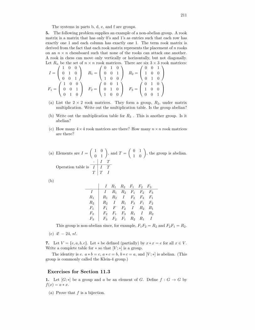
211
The systems in parts b, d, e, and f are groups.5. The following problem supplies an example of a non-abelian group. A rookmatrix is a matrix that has only 0’s and 1’s as entries such that each row hasexactly one 1 and each column has exactly one 1. The term rook matrix isderived from the fact that each rook matrix represents the placement of n rookson an n × n chessboard such that none of the rooks can attack one another.A rook in chess can move only vertically or horizontally, but not diagonally.Let Rn be the set of n × n rook matrices. There are six 3 × 3 rook matrices:
I =
1 0 0
0 1 0
0 0 1
R1 =
0 1 0
0 0 1
1 0 0
R2 =
0 0 1
1 0 0
0 1 0
F1 =
1 0 0
0 0 1
0 1 0
F2 =
0 0 1
0 1 0
1 0 0
F3 =
0 1 0
1 0 0
0 0 1
(a) List the 2 × 2 rook matrices. They form a group, R2, under matrix
multiplication. Write out the multiplication table. Is the group abelian?
(b) Write out the multiplication table for R3 . This is another group. Is itabelian?
(c) How many 4×4 rook matrices are there? How many n×n rook matricesare there?
(a) Elements are I =
(1 0
0 1
), and T =
(0 1
1 0
), the group is abelian.
Operation table is· I T
I I T
T T I
(b)I R1 R2 F1 F2 F3
I
R1
R2
F1
F2
F3
I R1 R2 F1 F2 F3
R1 R2 I F2 F3 F1
R2 I R1 F3 F1 F2
F1 F F2 I R2 R1
F2 F1 F3 R1 I R2
F3 F2 F1 R2 R1 I
This group is non-abelian since, for example, F1F2 = R2 and F2F1 = R2.
(c) 4! = 24, n!.
7. Let V = {e, a, b, c}. Let ∗ be defined (partially) by x ∗x = e for all x ∈ V .Write a complete table for ∗ so that [V ; ∗] is a group.
The identity is e. a ∗ b = c, a ∗ c = b, b ∗ c = a, and [V ; ∗] is abelian. (Thisgroup is commonly called the Klein-4 group.)
Exercises for Section 11.31. Let [G; ∗] be a group and a be an element of G. Define f : G → G byf(x) = a ∗ x.
(a) Prove that f is a bijection.
212APPENDIX B. HINTS AND SOLUTIONS TO SELECTED EXERCISES
(b) On the basis of part a, describe a set of bijections on the set of integers.
(a) f is injective:
f(x) = f(y)⇒ a ∗ x = a ∗ y⇒ x = y by left cancellation
.
f is surjective: For all b ∈ G, f(x) = b has the solution a−1 ∗ b.
(b) Functions of the form f(x) = a+x, where a is any integer, are bijections
3. Prove by induction on n that if a1, a2, . . ., an are elements of a group G,n ≥ 2, then (a1 ∗ a2 ∗ · · · ∗ an)
−1= a−1
n ∗ · · · ∗ a−12 ∗ a−1
1 . Interpret this resultin terms of [Z; +] and [R∗; ·].
Basis: (n = 2) (a1 ∗ a2)−1
= a−12 ∗ a
−11 by Theorem 11.3.7.
Induction: Assume that for some n ≥ 2,
(a1 ∗ a2 ∗ · · · ∗ an)−1
= a−1n ∗ · · · ∗ a−1
2 ∗ a−11
We must show that
(a1 ∗ a2 ∗ · · · ∗ an ∗ an+1)−1
= a−1n+1 ∗ a−1
n ∗ · · · ∗ a−12 ∗ a
−11
This can be accomplished as follows:
(a1 ∗ a2 ∗ · · · ∗ an ∗ an+1)−1
= ((a1 ∗ a2 ∗ · · · ∗ an) ∗ an+1)−1 by the associative law
= a−1n+1 ∗ (a1 ∗ a2 ∗ · · · ∗ an)
−1 by the basis
= a−1n+1 ∗
(a−1n ∗ · · · ∗ a−1
2 ∗ a−11
)by the induction hypothesis
= a−1n+1 ∗ a−1
n ∗ · · · ∗ a−12 ∗ a
−11 by the associative law
5. Prove Theorem 11.3.14.In this answer, we will refer to Lemma 11.3.13 simply as “the lemma.”
(a) Let p(n) be a−n =(a−1
)n, where a is any element of group [G; ∗]. Firstwe will prove that p(n) is true for all n ≥ 0.
Basis: If n = 0, Using the definition of the zero exponent,(a0)−1
=
e−1 = e, while(a−1
)0= e. Therefore, p(0) is true.
Induction: Assume that for some n ≥ 0, p(n) is true.(an+1
)−1= (an ∗ a)
−1 by the definition of exponentiation
= a−1 ∗ (an)−1 by the lemma
= a−1 ∗(a−1
)n by the induction hypothesis
=(a−1
)n+1 by the lemma
If n is negative, then −n is positive and
a−n =
(((a−1
)−1)−n)
=(a−1
)−(−n) since the property is true for positive numbers
=(a−1
)n
213
(b) For m > 1, let p(m) be an+m = an ∗ am for all n ≥ 1. The basis for thisproof follows directly from the basis for the definition of exponentiation.
Induction: Assume that for some m > 1, p(m) is true. Then
an+(m+1) = a(n+m)+1 by the associativity of integer addition
= an+m ∗ a1 by the definition of exponentiation
= (an ∗ am) ∗ a1 by the induction hypothesis
= an ∗(am ∗ a1
)by associativity
= an ∗ am+1 by the definition of exponentiation
To complete the proof, you need to consider the cases where m and/or nare negative.
(c) Let p(m)be (an)m
= anm for all integers n.
Basis: (am)0
= e and am·0 = a0 = e therefore, p(0) is true.
Induction; Assume that p(m) is true for some m >0,
(an)m+1
= (an)m ∗ an by the definition of exponentiation
= anm ∗ an by the induction hypothesis
= anm+n by part (b) of this proof
= an(m+1)
Finally, if m is negative, we can verify that (an)m
= anm using many ofthe same steps as the positive case.
Exercises for Section 11.41. Determine the greatest common divisors of the following pairs of integerswithout using any computational assistance.
(a) 23 · 32 · 5 and 22 · 3 · 52 · 7
(b) 7! and 3 · 5 · 7 · 9 · 11 · 13
(c) 194 and 195
(d) 12112 and 0
(a) 22 · 3 · 5
(b) 32 · 5 · 7
(c) 194
(d) 12112
3. Calculate:
(a) 7 +8 3
(b) 7×8 3
(c) 4×8 4
(d) 10 +12 2
214APPENDIX B. HINTS AND SOLUTIONS TO SELECTED EXERCISES
(e) 6×8 2 +8 6×8 5
(f) 6×8 (2 +8 5)
(g) 3×5 3×5 3×5 3 ≡ 34( mod5)
(h) 2×11 7
(i) 2×14 7
(a) 2
(b) 5
(c) 0
(d) 0
(e) 2
(f) 2
(g) 1
(h) 3
(i) 0
5. In the group Z11 , what are:
(a) 3(4)?
(b) 36(4)?
(c) How could you efficiently compute m(4), m ∈ Z?
(a) 1
(b) 1
(c) m(4) = r(4), wherem = 11q+r,0 ≤ r < 11
7. A student is asked to solve the following equations under the requirementthat all arithmetic should be done in Z2. List all solutions.
(a) x2 + 1 = 0.
(b) x2 + x+ 1 = 0.
Since the solutions, if they exist, must come from Z2, substitution is theeasiest approach.
(a) 1 is the only solution, since 12 +2 1 = 0 and 02 +2 1 = 1
(b) No solutions, since 02 +2 0 +2 1 = 1, and 12 +2 1 +2 1 = 1
10. Prove the division property, Theorem 11.4.1.Prove by induction on m that you can divide any positive integer into m.
That is, let p(m) be “For all n greater than zero, there exist unique integers qand r such that . . . .” In the induction step, divide n into m− n.11. Suppose f : Z17 → Z17 such f(i) = a×17 i+17 b where a and b are integerconstants. Furthermore, assume that f(1) = 11 and f(2) = 4. Find a formulafor f(i) and also find a formula for the inverse of f .
The given conditions can be converted to a system of linear equations:
f(1) = 11⇒ a+17 b = 11
f(2) = 4⇒ 2×17 a+17 b = 4
If we subtract the first equation from the second, we get a = 4 +17 (−11) =4 +17 6 = 10. This implies that b = 1, and f(i) = 10 × +17i + 1. To get a
215
formula for the inverse of f we solve f(j) = i for j, using the fact that themultiplicative inverse of 10 (mod 17) is 12.
f(j) = i⇒ 10×+17j + 1 = i
⇒ 10×+17j = i+17 16
⇒ j = 12×17 (i+17 16)
Therefore f−1(i) = 12×17 (i+17 16) = 12×17 i+17 5).
Exercises for Section 11.5
1. Which of the following subsets of the real numbers is a subgroup of [R; +]?
(a) the rational numbers
(b) the positive real numbers
(c) {k/2 | k is an integer}
(d) {2k | k is an integer}
(e) {x | −100 ≤ x ≤ 100}
Only a and c are subgroups.
3. Find at least two proper subgroups of R3 , the set of 3× 3 rook matrices(see Exercise 11.2.5).
{I,R1, R2}, {I, F1}, {I, F2}, and {I, F3} are all the proper subgroups ofR3.
5.
(a) List the cyclic subgroups of Z6 and draw an ordering diagram for therelation “is a subset of” on these subgroups.
(b) Do the same for Z12.
(c) Do the same for Z8.
(d) On the basis of your results in parts a, b, and c, what would you expectif you did the same with Z24?
(a) 〈1〉 = 〈5〉 = Z6, 〈2〉 = 〈4〉 = {2, 4, 0}, 〈3〉 = {3, 0}, 〈0〉 = {0}
(b) 〈1〉 = 〈5〉 = 〈7〉 = 〈11〉 = Z12, 〈2〉 = 〈10〉 = {2, 4, 6, 8, 10, 0}, 〈3〉 = 〈9〉 ={3, 6, 9, 0}, 〈4〉 = 〈8〉 = {4, 8, 0}, 〈6〉 = {6, 0}, 〈0〉 = {0}
(c) 〈1〉 = 〈3〉 = 〈5〉 = 〈7〉 = Z8, 〈2〉 = 〈6〉 = {2, 4, 6, 0}, 〈4〉 = {4, 0},〈0〉 = {0}
(d) Based on the ordering diagrams for parts a through c in Figure B.0.1, wewould expect to see an ordering diagram similar to the one for divideson {1, 2, 3, 4, 6, 8, 12, 24} (the divisors of 24) if we were to examine thesubgroups of Z24. This is indeed the case.
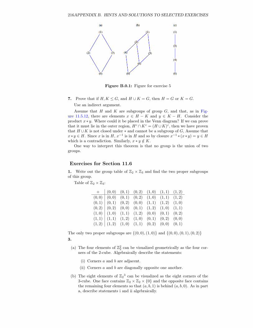
216APPENDIX B. HINTS AND SOLUTIONS TO SELECTED EXERCISES
Figure B.0.1: Figure for exercise 5
7. Prove that if H,K ≤ G, and H ∪K = G, then H = G or K = G.Use an indirect argument.Assume that H and K are subgroups of group G, and that, as in Fig-
ure 11.5.12, there are elements x ∈ H − K and y ∈ K − H. Consider theproduct x ∗ y. Where could it be placed in the Venn diagram? If we can provethat it must lie in the outer region, Hc ∩Kc = (H ∪K)c, then we have proventhat H ∪K is not closed under ∗ and cannot be a subgroup of G, Assume thatx ∗ y ∈ H. Since x is in H, x−1 is in H and so by closure x−1 ∗ (x ∗ y) = y ∈ Hwhich is a contradiction. Similarly, x ∗ y /∈ K.
One way to interpret this theorem is that no group is the union of twogroups.
Exercises for Section 11.6
1. Write out the group table of Z2 × Z3 and find the two proper subgroupsof this group.
Table of Z2 × Z3:
+ (0, 0) (0, 1) (0, 2) (1, 0) (1, 1) (1, 2)
(0, 0) (0, 0) (0, 1) (0, 2) (1, 0) (1, 1) (1, 2)
(0, 1) (0, 1) (0, 2) (0, 0) (1, 1) (1, 2) (1, 0)
(0, 2) (0, 2) (0, 0) (0, 1) (1, 2) (1, 0) (1, 1)
(1, 0) (1, 0) (1, 1) (1, 2) (0, 0) (0, 1) (0, 2)
(1, 1) (1, 1) (1, 2) (1, 0) (0, 1) (0, 2) (0, 0)
(1, 2) (1, 2) (1, 0) (1, 1) (0, 2) (0, 0) (0, 1)
The only two proper subgroups are {(0, 0), (1, 0)} and {(0, 0), (0, 1), (0, 2)}3.
(a) The four elements of Z22 can be visualized geometrically as the four cor-
ners of the 2-cube. Algebraically describe the statements:
(i) Corners a and b are adjacent.
(ii) Corners a and b are diagonally opposite one another.
(b) The eight elements of Z23 can be visualized as the eight corners of the
3-cube. One face contains Z2 × Z2 × {0} and the opposite face containsthe remaining four elements so that (a, b, 1) is behind (a, b, 0). As in parta, describe statements i and ii algebraically.
217
(c) If you could imagine a geometric figure similar to the square or cube inn dimensions, and its comers were labeled by elements of Z2
n as in partsa and b, how would statements i and ii be expressed algebraically?
(a) (i) a+ b could be (1, 0) or (0, 1). (ii) a+ b = (1, 1).
(b) (i) a+ b could be(1, 0, 0), (0, 1, 0), or (0, 0, 1). (ii) a+ b = (1, 1, 1).
(c) (i) a+ b has exactly one 1. (ii) a+ b has all 1′s.
5. Which of the following sets are subgroups of Z×Z? Give a reason for anynegative answers.
(a) {0}
(b) {(2j, 2k) | j, k ∈ Z}
(c) {(2j + 1, 2k) | j, k ∈ Z}
(d) {(n, n2) | n ∈ Z}
(e) {(j, k) | j + k is even}
(a) No, 0 is not an element of Z× Z.
(b) Yes.
(c) No, (0, 0) is not an element of this set.
(d) No, the set is not closed: (1, 1) + (2, 4) = (3, 5) and (3, 5) is not in theset.
(e) Yes.
Exercises for Section 11.71. State whether each pair of groups below is isomorphic. For each pair thatis, give an isomorphism; for those that are not, give your reason.
(a) Z× R and R× Z
(b) Z2 × Z and Z× Z
(c) R and Q×Q
(d) P({1, 2}) with symmetric difference and Z22
(e) Z22 and Z4
(f) R4 and M2×2(R) with matrix addition
(g) R2 and R× R+
(h) Z2 and the 2× 2 rook matrices
(i) Z6 and Z2 × Z3
218APPENDIX B. HINTS AND SOLUTIONS TO SELECTED EXERCISES
(a) Yes, f(n, x) = (x, n) for (n, x) ∈ Z× R is an isomorphism.
(b) No, Z2 × Z has a two element subgroup while Z× Z does not.
(c) No. Q × Q is countable and R is not. Therefore, no bijection can existbetween them.
(d) Yes.
(e) No.
(f) Yes, one isomorphism is defined by f (a1, a2, a3, a4) =
(a1 a2
a3 a4
).
(g) Yes, one isomorphism is defined by f (a1, a2) = (a1, 10a2).
(h) Yes.
(i) Yes f(k) = k(1, 1).
3. Prove that the relation “is isomorphic to” on groups is transitive.Consider three groups G1, G2, and G3 with operations ∗, �, and ?, respec-
tively. We want to show that if G1 is isomorphic to G2, and if G2 is isomorphicto G3 , then G1 is isomorphic to G3.
G1 isomorphic to G2 ⇒ there exists an isomorphism f : G1 → G2
G2 isomorphic to G3 ⇒ there exists an isomorphism g : G2 → G3
If we compose g with f , we get the function g◦f : G1 → G3, By Theorem 7.0.1and Theorem 7.0.2, g ◦ f is a bijection, and if a, b ∈ G1,
(g ◦ f)(a ∗ b) = g(f(a ∗ b))= g(f(a) � f(b)) since f is an isomorphism= g(f(a)) ? g(f(b)) since g is an isomorphism= (g ◦ f)(a) ? (g ◦ f)(b)
Therefore, g◦f is an isomorphism from G1 into G3, proving that “is isomorphicto” is transitive.5. The two groups [Z4; +4] and [U5;×5] are isomorphic. One isomorphismT : Z4 → U5 is partially defined by T (1) = 3. Determine the values of T (0),T (2), and T (3).
By Theorem 11.7.14(a), T (0) must be 1. T (2) = T (1+41) = T (1)×5T (1) =3×5 3 = 4. Since T is a bijection, T (3) = 2.7. Prove that all infinite cyclic groups are isomorphic to Z.
Let G be an infinite cyclic group generated by a. Then, using multiplicativenotation, G = {an|n ∈ Z}. The map T : G → Z defined by T (an) = n isan isomorphism. This is indeed a function, since an = am implies n = m.Otherwise, a would have a finite order and would not generate G.
(a) T is one-to-one, since T (an) = T (am) implies n = m, so an = am.
(b) T is onto, since for any n ∈ Z, T (an) = n.
(c) T (an ∗ am) = T (an+m) = n+m = T (an) + T (am)
10. It can be shown that there are five non-isomorphic groups of order eight.You should be able to describe at least three of them. Do so without use oftables. Be sure to explain why they are not isomorphic.Z8, Z2 × Z4 , and Z3
2. One other is the fourth dihedral group, introducedin Section 15.3.
219
Exercises for Section 12.11. Solve the following systems by describing the solution sets completely:
(a) 2x1 + x2 = 3
x1 − x2 = 1
(b)2x1 + x2 + 3x3 = 5
4x1 + x2 + 2x3 = −1
8x1 + 2x2 + 4x3 = −2
(c)x1 + x2 + 2x3 = 1
x1 + 2x2 − x3 = −1
x1 + 3x2 + x3 = 5
(d) x1 − x2 + 3x3 = 7
x1 + 3x2 + x3 = 4
(a) {(4/3, 1/3)}
(b) {( 12x3 − 3,−4x3 + 11, x3) | x3 ∈ R}
(c) {(−5, 14/5, 8/5)}
(d) {(6.25− 2.5x3,−0.75 + 0.5x3, x3) | x3 ∈ R}
3. Given the final augmented matrices below from the Gauss-Jordan Algo-rithm, identify the solutions sets. Identify the basic and free variables, anddescribe the solution set of the original system.
(a)
1 0 −5 0 1.2
0 1 4 0 2.6
0 0 0 1 4.5
(b)
1 0 9 3
0 1 0 4
0 0 0 1
(c)
1 0 6 5
0 1 −2 1
0 0 0 0
(d)
1 0 0 −3 1
0 1 0 2 2
0 0 1 −1 1
(a) Basic variables: x1, x2 and x4. Free variable: x3. Solution set: {(1.2 +5x3, 2.6− 4x3, 4.5) | x3 ∈ R}
(b) Basic variables: x1 and x2. Free variable: x3. The solution set is emptybecause the last row of the matrix converts to the inconsistent equation0 = 1.
(c) Basic variables: x1 and x2. Free variable: x3. Solution set: {(−6x3 + 5, 2x3 + 1, x3) | x3 ∈ R}
(d) Basic variables: x1, x2 and x3. Free variable: x4. Solution set: {(3x4 + 1,−2x4 + 2, x4 + 1, x4) | x4 ∈ R}
5. Solve the following systems using only mod 5 arithmetic. Your solutionsshould be n− tuples from Z5.
(a) 2x1 + x2 = 3
x1 + 4x2 = 1(compare your solution to the system in 5(a))
(b)x1 + x2 + 2x3 = 1
x1 + 2x2 + 4x3 = 4
x1 + 3x2 + 3x3 = 0
(a) {(3, 0)}
220APPENDIX B. HINTS AND SOLUTIONS TO SELECTED EXERCISES
(b) {(3, 0, 4)}
7. Given a system of n linear equations in n unknowns in matrix form AX =b, prove that if b is a matrix of all zeros, then the solution set of AX = b is asubgroup of Rn.
Proof: Since b is the n× 1 matrix of 0’s, let’s call it 000. Let S be the set ofsolutions to AX = 000. If X1 and X2 be in S. Then
A (X1 +X2) = AX1 +AX2 = 000 + 000 = 000
so X1 +X2 ∈ S; or in other words, S is closed under addition in Rn.The identity of Rn is 000, which is in S. Finally, let X be inS. Then
A(−X) = −(AX) = −000 = 000
and so −X is also in S.
Exercises for Section 12.2
3. Use the method of this section to find the inverses of the following matriceswhenever possible. If an inverse does not exist, explain why.
(a)(
13 215 −1
)
(b)
1 0 0 3
2 −1 0 6
0 2 1 0
0 −1 3 2
(c)
1 −1 0
−1 2 −1
0 −1 1
(d)
1 0 0
2 2 −1
1 −1 1
(e)
2 3 4
3 4 5
4 5 6
(f)
1 12
13
12
13
14
13
14
15
(a)(
1511
3011
311 − 5
11
)
(b)
−20 21
292 − 3
2
2 −1 0 0
−4 2 1 0
7 − 72 − 3
212
221
(c) The inverse does not exist. When the augmented matrix is row-reduced(see below), the last row of the first half cannot be manipulated to matchthe identity matrix.
(d)
1 0 0
−3 1 1
−4 1 2
(e) The inverse does not exist.
(f)
9 −36 30
−36 192 −180
30 −180 180
5. Express each system of equations in Exercise 12.1.1 in the form Ax = B.When possible, solve each system by first finding the inverse of the matrix ofcoefficients.
The solutions are in the solution section of Section 12.1, exercise 1, Weillustrate with the outline of the solution to part (c). The matrix version ofthe system is 1 1 2
1 2 −1
1 3 1
x1
x2
x3
=
1
−1
5
We compute the inverse of the matrix of coefficients and get
A−1 =
1 1 2
1 2 −1
1 3 1
−1
=1
5
5 5 −5
−2 −1 3
1 −2 1
and x1
x2
x3
= A−1
1
−1
5
=
−514585
Exercises for Section 12.33.
(a) Verify that M2×3 (R) is a vector space over R. What is its dimension?
(b) Is Mm×n (R) a vector space over R? If so, what is its dimension?
The dimension of M2×3 (R) is 6 and yes, Mm×n (R) is also a vector spaceof dimension m · n. One basis for Mm×n (R) is {Aij | 1 ≤ i ≤ m, 1 ≤ j ≤ n}where Aij is the m× n matrix with entries all equal to zero except for in rowi, column j where the entry is 1.
7. Express the vector(
1 2
−3 3
)∈ M2×2(R), as a linear combination of(
1 1
1 1
),(−1 5
2 1
),(
0 1
1 1
)and
(0 0
0 1
)If the matrices are named B, A1, A2 , A3, and A4 , then
B =8
3A1 +
5
3A2 +
−5
3A3 +
23
3A4
9.
222APPENDIX B. HINTS AND SOLUTIONS TO SELECTED EXERCISES
(a) Show that the set {x1,x2} generates R2 for each of the parts in Exercise6 of this section.
(b) Show that {x1,x2,x3} generates R2 where x1 = (1, 1), x2 = (3, 4), andx3 = (−1, 5).
(c) Create a set of four or more vectors that generates R2.
(d) What is the smallest number of vectors needed to generate R2? Rn?
(e) Show that the set
{A1, A2, A3, A4} = {(
1 0
0 0
),
(0 1
0 0
),
(0 0
1 0
),
(0 0
0 1
)}
generates M2×2(R)
(f) Show that{
1, x, x2, x3}generates P 3.
(a) If x1 = (1, 0), x2 = (0, 1), and y = (b1, b2), then y = b1x1 + b2x2. Ifx1 = (3, 2), x2 = (2, 1), and y = (b1, b2), then y = (−b1 + 2b2)x1 +(2b1 − 3b2)x2.
(b) If y = (b1, b2) is any vector in R2 , then y = (−3b1 + 4b2)x1+(−b1 + b2)x2+(0)x3
(c) One solution is to add any vector(s) to x1, x2, and x3 of part b.
(d) 2, n
(e)(x y
z w
)= xA1 + yA2 + zA3 + wA4
(f) a0 + a1x+ a2x2 + a3x
3 = a0(1) + a1(x) + a2
(x2)
+ a3
(x3).
11.
(a) Prove that {(4, 1), (1, 3)} is a basis for R2 over R.
(b) Prove that {(1, 0), (3, 4)} is a basis for R2 over R.
(c) Prove that {(1, 0,−1), (2, 1, 1), (1,−3,−1)} is a basis for R3 over R.
(d) Prove that the sets in Exercise 9, parts e and f, form bases of the respec-tive vector spaces.
(a) The set is linearly independent: let a and b be scalars such that a(4, 1) +b(1, 3) = (0, 0), then 4a + b = 0 and a + 3b = 0 which has a = b = 0 asits only solutions. The set generates all of R2: let (a, b) be an arbitraryvector in R2 . We want to show that we can always find scalars β1 and β2
such that β1(4, 1) +β2(1, 3) = (a, b). This is equivalent to finding scalarssuch that 4β1 + β2 = a and β1 + 3β2 = b. This system has a uniquesolution β1 = 3a−b
11 , and β2 = 4b−a11 . Therefore, the set generates R2.
13.
(a) Let y1 = (1, 3, 5, 9), y2 = (5, 7, 6, 3), and c = 2. Find y1 + y2 and cy1.
223
(b) Let f1(x) = 1 + 3x+ 5x2 + 9x3 , f2(x) = 5 + 7x+ 6x2 + 3x3 and c = 2.Find f1(x) + f2(x) and cf1(x).
(c) Let A =
(1 3
5 9
), B =
(5 7
6 3
), and c = 2. Find A+B and cA.
(d) Are the vector spaces R4 , P 3 and M2×2(R) isomorphic to each other?Discuss with reference to previous parts of this exercise.
The answer to the last part is that the three vector spaces are all isomorphicto one another. Once you have completed part (a) of this exercise, the followingtranslation rules will give you the answer to parts (b) and (c),
(a, b, c, d)↔(a b
c d
)↔ a+ bx+ cx2 + dx2
Exercises for Section 12.41.
(a) List three different eigenvectors of A =
(2 1
2 3
), the matrix of Exam-
ple 12.4.2, associated with each of the two eigenvalues 1 and 4. Verifyyour results.
(b) Choose one of the three eigenvectors corresponding to 1 and one of thethree eigenvectors corresponding to 4, and show that the two chosenvectors are linearly independent.
(a) Any nonzero multiple of(
1
−1
)is an eigenvector associated with λ = 1.
(b) Any nonzero multiple of(
1
2
)is an eigenvector associated with λ = 4.
(c) Let x1 =
(a
−a
)and x2 =
(b
2b
). You can verify that c1x1 +
c2x2 =
(0
0
)if and only if c1 = c2 = 0. Therefore, {x1, x2} is linearly
independent.
3.
(a) Verify that P−1AP is indeed equal to(
1 0
0 4
), as indicated in Exam-
ple 12.4.6
(b) Choose P (1) =
(1
2
)and P (2) =
(1
−1
)and verify that the new value
of P satisfies P−1AP =
(4 0
0 1
)(c) Take any two linearly independent eigenvectors of the matrix A of Ex-
ample 12.4.6 and verify that P−1AP is a diagonal matrix.
224APPENDIX B. HINTS AND SOLUTIONS TO SELECTED EXERCISES
Part c: You should obtain(
4 0
0 1
)or(
1 0
0 4
), depending on how you
order the eigenvalues.5. Diagonalize the following, if possible:
(a)(
1 2
3 2
)
(b)(−2 1
−7 6
)(c)
(3 0
0 4
)
(d)
1 −1 4
3 2 −1
2 1 −1
(e)
6 0 0
0 7 −4
9 1 3
(f)
1 −1 0
−1 2 −1
0 −1 1
(a) If P =
(2 1
3 −1
), then
P−1AP =
(4 0
0 −1
).
(b) If P =
(1 1
7 1
), then
P−1AP =
(5 0
0 −1
).
(c) If P =
(1 0
0 1
), then
P−1AP =
(3 0
0 4
).
(d) If P =
1 −1 1
−1 4 2
−1 1 1
, then
P−1AP =
−2 0 0
0 1 0
0 0 0
.
(e) A is not diagonalizable. Five is adouble root of the characteristicequation, but has an eigenspacewith dimension only 1.
(f) If P =
1 1 1
−2 0 1
1 −1 1
, then
P−1AP =
3 0 0
0 1 0
0 0 0
.
7. Let A and P be as in Example 12.4.8. Show that the columns of the matrixAP can be found by computing AP (1), AP (2), . . . , AP (n).
This is a direct application of the definition of matrix multiplication. LetA(i) be the ith row of A, and let P (j) be the jth column of P . Then the jthcolumn of the product AP is
A(1)P(j)
A(2)P(j)
...A(n)P
(j)
Hence, (AP )(j) = A
(P (j)
)for j = 1, 2, . . . , n. Thus, each column of AP
depends on A and the j th column of P .
Exercises for Section 12.5
4. How many paths are there of length 6 from vertex 1 to vertex 3 in Fig-ure B.0.2? How many paths from vertex 2 to vertex 2 of length 6 are there?
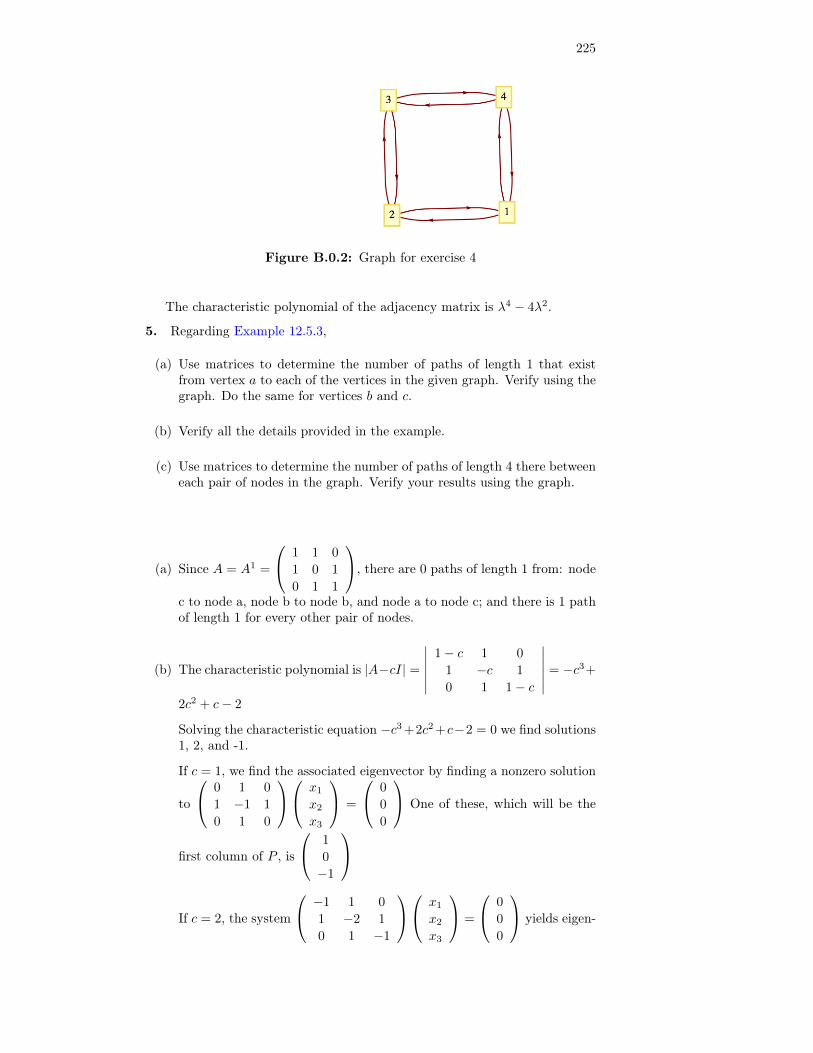
225
Figure B.0.2: Graph for exercise 4
The characteristic polynomial of the adjacency matrix is λ4 − 4λ2.
5. Regarding Example 12.5.3,
(a) Use matrices to determine the number of paths of length 1 that existfrom vertex a to each of the vertices in the given graph. Verify using thegraph. Do the same for vertices b and c.
(b) Verify all the details provided in the example.
(c) Use matrices to determine the number of paths of length 4 there betweeneach pair of nodes in the graph. Verify your results using the graph.
(a) Since A = A1 =
1 1 0
1 0 1
0 1 1
, there are 0 paths of length 1 from: node
c to node a, node b to node b, and node a to node c; and there is 1 pathof length 1 for every other pair of nodes.
(b) The characteristic polynomial is |A−cI| =
∣∣∣∣∣∣1− c 1 0
1 −c 1
0 1 1− c
∣∣∣∣∣∣ = −c3+
2c2 + c− 2
Solving the characteristic equation −c3 +2c2 +c−2 = 0 we find solutions1, 2, and -1.
If c = 1, we find the associated eigenvector by finding a nonzero solution
to
0 1 0
1 −1 1
0 1 0
x1
x2
x3
=
0
0
0
One of these, which will be the
first column of P , is
1
0
−1
If c = 2, the system
−1 1 0
1 −2 1
0 1 −1
x1
x2
x3
=
0
0
0
yields eigen-
226APPENDIX B. HINTS AND SOLUTIONS TO SELECTED EXERCISES
vectors, including
1
1
1
, which will be the second column of P .
If c = −1, then the system determining the eigenvectors is
2 1 0
1 1 1
0 1 2
x1
x2
x3
=
0
0
0
and we can select
1
−2
1
, although any nonzero multiple of
this vector could be the third column of P .
(c) Assembling the results of part (b) we have P =
1 1 1
0 1 −2
−1 1 1
.
A4 = P
14 0 0
0 24 0
0 0 (−1)4
P−1 = P
1 0 0
0 16 0
0 0 1
P−1
=
1 16 1
0 16 −2
−1 16 1
12 0 − 1
213
13
13
16 − 1
316
=
6 5 5
5 6 5
5 5 6
Hence there are five different paths of length 4 between distinct vertices,and six different paths that start and end at the same vertex. The readercan verify these facts from Figure 12.5.4
7. We noted in Chapter 5 that since matrix algebra is not commutative un-
der multiplication, certain difficulties arise. Let A =
(1 1
0 0
)and B =(
0 0
0 2
).
(a) Compute eA, eB , and eA+B . Compare eAeB , eBeA and eA+B .
(b) Show that if 000 is the 2× 2 zero matrix, then e000 = I.
(c) Prove that if A and B are two matrices that do commute, then eA+B =eAeB , thereby proving that eA and eB commute.
(d) Prove that for any matrix A,(eA)−1
= e−A.
(a) eA =
(e e
0 0
), eB =
(0 0
0 e2
), and eA+B =
(e e2 − e0 e2
)(b) Let 000 be the zero matrix, e000 = I + 000 + 0002
2 + 0003
6 + . . . = I .
(c) Assume that A and B commute. We will examine the first few termsin the product eAeB . The pattern that is established does continue ingeneral. In what follows, it is important that AB = BA. For example, in
227
the last step, (A+B)2 expands to A2+AB+BA+B2, not A2+2AB+B2,if we can’t assume commutativity.
eAeB =
( ∞∑k=0
Ak
k!
)( ∞∑k=0
Bk
k!
)
=
(I +A+
A2
2+A3
6+ · · ·
)(I +B +
B2
2+B3
6+ · · ·
)= I +A+B +
A2
2+AB +
B2
2+A3
6+A2B
2+AB2
2+B3
6+ · · ·
= I + (A+B) +1
2
(A2 + 2AB +B2
)+
1
6
(A3 + 3A2B + 3AB2 +B3
)+ · · ·
= I + (A+B) +1
2(A+B)2 +
1
6(A+B)3 + · · ·
= eA+B
(d) Since A and −A commute, we can apply part d;
eAe−A = eA+(−A) = e000 = I
Exercises for this section
1. Solve the following systems, describing the solution sets completely:
(a) x1 + x2 = 0
x1 + x3= 0 (b)
x1 + x2 = 0
x2 + x3 = 0
x3 + x4= 1
x1 + x2 + x3 = 1
(a) {(0, 0, 0), (1, 1, 1)}
(b) {(1, 1, 1, 0)}
2. This exercise provides an example in which the number of basic variables isless than the number of equations. The only difference between the two systemsbelow is the right hand sides. You can start with an augmented matrix havingto right side columns and do row reduction for both systems at the same time.
(a)x1 + x2 + x4= 1
x1 + x3 + x4= 0
x2 + x3 = 1
(b)x1 + x2 + x4= 1
x1 + x3 + x4= 0
x2 + x3 = 0
As suggested here is the augmented matrix with both right sides, and it’srow reduction: 1 1 0 1 1 1
1 0 1 1 0 0
0 1 1 0 1 0
−→
1 0 1 1 0 0
0 1 1 0 1 0
0 0 0 0 0 1
There are only two basic variables here because the left side of the last equationis the sum of the left sides of the first two equations.
228APPENDIX B. HINTS AND SOLUTIONS TO SELECTED EXERCISES
(a) Ignoring the last column of both matrices, we see that the last equationof the first system reduces to 0 = 0, which is always true, and the firsttwo equations yield two free variables, x3 and x4. The general solutionis the set of quadruples {(x3 +2 x4, x3 +2 1, x3, x4) | x3, x4 ∈ Z2}. Thecardinality of the the solution set is 4.
(b) If we replace the fifth column with the sixth one, the last row indicatesthat 0 = 1, which means that the solution set is empty.
3. This exercise motivates the concept of a coset in Chapter 15.
(a) Solve the following system and prove that the solution set is a linearcombination of vectors in Z5
2 and also a subgroup of the group Z52 under
coordinatewise mod 2 addition.
x1 + x2 + x5= 0
x1 + x3 + x5= 0
x1 + x3 + x4 = 0
x2 + x3 + x4 = 0
(b) Describe the solution set to the following system as it relates to thesolution set to the system in the previous part of this exercise.
x1 + x2 + x5= 1
x1 + x3 + x5= 0
x1 + x3 + x4 = 1
x2 + x3 + x4 = 0
(a) Row reduction produces a solution with one free variable, x3.
(x1, x2, x3, x4, x5) = (x3, x3, x3, 0, 0)
= x3(1, 1, 1, 0, 0)
The solution set has only two elements. It is {(0, 0, 0, 0, 0), (1, 1, 1, 0, 0)}.Since Z5
2 is a finite group, the solution set is a subgroup because it isclosed with respect to coordinate-wise mod 2 addition.
(b) The row-reduced augmented matrix of coefficients provides the solution
(x1, x2, x3, x4, x5) = (x3, 1 + x3, x3, 1, 0)
= (0, 1, 0, 1, 0) + x3(1, 1, 1, 0, 0)
Therefore, the solution to this system is a shift of the solution set to thehomogeneous system by the vector (0, 1, 0, 1, 0), which is {(0, 1, 0, 1, 0), (1, 0, 1, 1, 0)}
Exercises for Section 13.11. Consider the poset (D30, |), where D30 = {1, 2, 3, 5, 6, 10, 15, 30}.
(a) Find all lower bounds of 10 and 15.
(b) Find the greatest lower bound of 10 and 15.
(c) Find all upper bounds of 10 and 15.
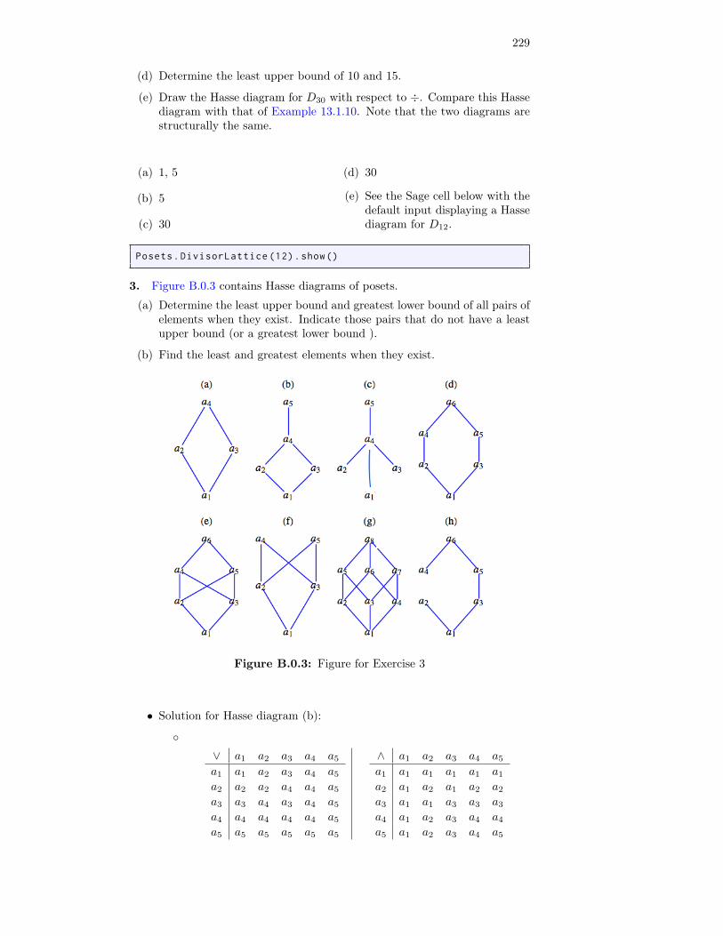
229
(d) Determine the least upper bound of 10 and 15.
(e) Draw the Hasse diagram for D30 with respect to ÷. Compare this Hassediagram with that of Example 13.1.10. Note that the two diagrams arestructurally the same.
(a) 1, 5
(b) 5
(c) 30
(d) 30
(e) See the Sage cell below with thedefault input displaying a Hassediagram for D12.
Posets.DivisorLattice (12).show()
3. Figure B.0.3 contains Hasse diagrams of posets.
(a) Determine the least upper bound and greatest lower bound of all pairs ofelements when they exist. Indicate those pairs that do not have a leastupper bound (or a greatest lower bound ).
(b) Find the least and greatest elements when they exist.
Figure B.0.3: Figure for Exercise 3
• Solution for Hasse diagram (b):
◦∨ a1 a2 a3 a4 a5
a1 a1 a2 a3 a4 a5
a2 a2 a2 a4 a4 a5
a3 a3 a4 a3 a4 a5
a4 a4 a4 a4 a4 a5
a5 a5 a5 a5 a5 a5
∧ a1 a2 a3 a4 a5
a1 a1 a1 a1 a1 a1
a2 a1 a2 a1 a2 a2
a3 a1 a1 a3 a3 a3
a4 a1 a2 a3 a4 a4
a5 a1 a2 a3 a4 a5
230APPENDIX B. HINTS AND SOLUTIONS TO SELECTED EXERCISES
a1 is the least element and a5 is the greatest element.
• Partial solution for Hasse diagram (f):
◦ lub (a2, a3) and lub (a4, a5) do not exist.
◦ No greatest element exists, but a1 is the least element.
5.
(a) Prove the second part of Theorem 13.1.6, the least upper bound of twoelements in a poset is unique, it one exists.
(b) Prove that if a poset L has a least element, then that element is unique.
If 0 and 0′ are distinct least elements, then
0 ≤ 0′ since 0 is a least element0′ ≤ 0 since 0′ is a least element
}⇒ 0 = 0′ by antisymmetry, a contradiction
Exercises for Section 13.25. What is a reasonable definition of the term sublattice?
One reasonable definition would by this: Let [L;∨,∧] be a lattice and letK be a nonempty subset of L. Then K is a sublattice of L if and only if K isclosed under both ∨ and ∧
Exercises for Section 13.31. Determine the complement of each element B ∈ L in Example 13.3.4. Isthis lattice a Boolean algebra? Why?
B Complement of B∅{a}{b}{c}{a, b}{a, c}{b, c}A
A
{b, c}{a, c}{a, b}{c}{b}{a}∅
This lattice is a Boolean algebra since it is a distributive complementedlattice.3. Determine which of the lattices of Exercise 13.1.3 of Section 13.1 areBoolean algebras.
a and g.5. It can be shown that the following statement, S, holds for any Booleanalgebra [B;∨,∧,−] : (a ∧ b) = a if and only if a ≤ b.
(a) Write the dual, S∗, of the statement S.
(b) Write the statement S and its dual, S∗, in the language of sets.
(c) Are the statements in part b true for all sets?
(d) Write the statement S and its dual, S∗, in the language of logic.
231
(e) Are the statements in part d true for all propositions?
(a) S∗ : a ∨ b = a if a ≥ b
(b) The dual of S : A ∩B = A if A ⊆ B is S∗ : A ∪B = A if A ⊇ B
(c) Yes
(d) The dual of S : p ∧ q ⇔ p if p⇒ q is S∗ : p ∨ q ⇔ p if q ⇒ p
(e) Yes
7. Formulate a definition for isomorphic Boolean algebras.
[B;∧,∨,−] is isomorphic to [B′;∧,∨, ] if and only if there exists a functionT : B → B′ such that
(a) T is a bijection;
(b) T (a ∧ b) = T (a) ∧ T (b) for all a, b ∈ B
(c) T (a ∨ b) = T (a) ∨ T (b) for all a, b ∈ B
(d) T (a) = ˜T (a) for all a ∈ B.
Exercises for Section 13.4
1.
(a) Show that a = 2 is an atom of the Boolean algebra [D30;∨,∧,−].
(b) Repeat part a for the elements 3 and 5 of D30.
(c) Verify Theorem Theorem 13.4.5 for the Boolean algebra [D30;∨,∧,−].
(a) For a = 3 we must show that for each x ∈ D30 one of the following istrue: x ∧ 3 = 3 or x ∧ 3 = 1. We do this through the following table:
x verification1
2
3
5
6
10
15
30
1 ∧ 3 = 1
2 ∧ 3 = 1
3 ∧ 3 = 3
5 ∧ 3 = 1
6 ∧ 3 = 3
20 ∧ 3 = 1
15 ∧ 3 = 3
30 ∧ 3 = 3
For a = 5, a similar verification can be performed.
(b) 6 = 2 ∨ 3, 10 = 2 ∨ 5, 15 = 3 ∨ 5, and 30 = 2 ∨ 3 ∨ 5.
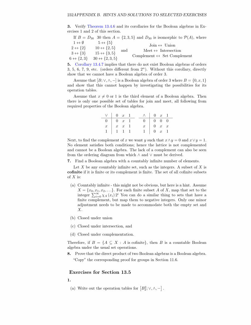
232APPENDIX B. HINTS AND SOLUTIONS TO SELECTED EXERCISES
3. Verify Theorem 13.4.6 and its corollaries for the Boolean algebras in Ex-ercises 1 and 2 of this section.
If B = D30 30 then A = {2, 3, 5} and D30 is isomorphic to P(A), where1↔ ∅ 5↔ {5}
2↔ {2} 10↔ {2, 5}3↔ {3} 15↔ {3, 5}
6↔ {2, 3} 30↔ {2, 3, 5}
andJoin↔ Union
Meet↔ IntersectionComplement↔ Set Complement
5. Corollary 13.4.7 implies that there do not exist Boolean algebras of orders3, 5, 6, 7, 9, etc. (orders different from 2n). Without this corollary, directlyshow that we cannot have a Boolean algebra of order 3.
Assume that [B;∨,∧,−] is a Boolean algebra of order 3 where B = {0, x, 1}and show that this cannot happen by investigating the possibilities for itsoperation tables.
Assume that x 6= 0 or 1 is the third element of a Boolean algebra. Thenthere is only one possible set of tables for join and meet, all following fromrequired properties of the Boolean algebra.
∨ 0 x 1
0
x
1
0 x 1
x x 1
1 1 1
∧ 0 x 1
0
x
1
0 0 0
0 x x
0 x 1
Next, to find the complement of x we want y such that x∧y = 0 and x∨y = 1.No element satisfies both conditions; hence the lattice is not complementedand cannot be a Boolean algebra. The lack of a complement can also be seenfrom the ordering diagram from which ∧ and ∨ must be derived.7. Find a Boolean algebra with a countably infinite number of elements.
Let X be any countably infinite set, such as the integers. A subset of X iscofinite if it is finite or its complement is finite. The set of all cofinite subsetsof X is:
(a) Countably infinite - this might not be obvious, but here is a hint. AssumeX = {x0, x1, x2, . . .}. For each finite subset A of X, map that set to theinteger
∑∞i=0 χA (xi) 2i You can do a similar thing to sets that have a
finite complement, but map them to negative integers. Only one minoradjustment needs to be made to accommodate both the empty set andX.
(b) Closed under union
(c) Closed under intersection, and
(d) Closed under complementation.
Therefore, if B = {A ⊆ X : A is cofinite}, then B is a countable Booleanalgebra under the usual set operations.8. Prove that the direct product of two Boolean algebras is a Boolean algebra.
“Copy” the corresponding proof for groups in Section 11.6.
Exercises for Section 13.51.
(a) Write out the operation tables for[B2
2 ;∨,∧,−].
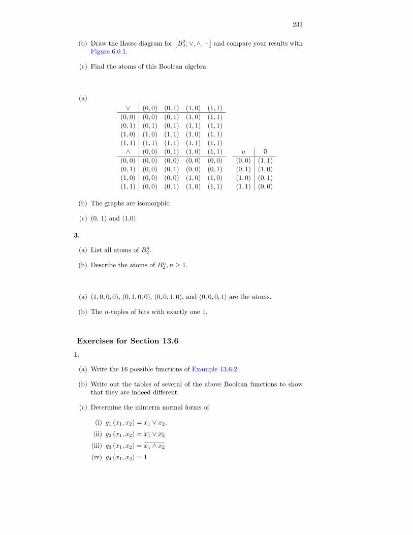
233
(b) Draw the Hasse diagram for[B2
2 ;∨,∧,−]and compare your results with
Figure 6.0.1.
(c) Find the atoms of this Boolean algebra.
(a)∨ (0, 0) (0, 1) (1, 0) (1, 1)
(0, 0) (0, 0) (0, 1) (1, 0) (1, 1)
(0, 1) (0, 1) (0, 1) (1, 1) (1, 1)
(1, 0) (1, 0) (1, 1) (1, 0) (1, 1)
(1, 1) (1, 1) (1, 1) (1, 1) (1, 1)
∧ (0, 0) (0, 1) (1, 0) (1, 1)
(0, 0) (0, 0) (0, 0) (0, 0) (0, 0)
(0, 1) (0, 0) (0, 1) (0, 0) (0, 1)
(1, 0) (0, 0) (0, 0) (1, 0) (1, 0)
(1, 1) (0, 0) (0, 1) (1, 0) (1, 1)
u___u
(0, 0) (1, 1)
(0, 1) (1, 0)
(1, 0) (0, 1)
(1, 1) (0, 0)
(b) The graphs are isomorphic.
(c) (0, 1) and (1,0)
3.
(a) List all atoms of B42 .
(b) Describe the atoms of Bn2 , n ≥ 1.
(a) (1, 0, 0, 0), (0, 1, 0, 0), (0, 0, 1, 0), and (0, 0, 0, 1) are the atoms.
(b) The n-tuples of bits with exactly one 1.
Exercises for Section 13.6
1.
(a) Write the 16 possible functions of Example 13.6.2.
(b) Write out the tables of several of the above Boolean functions to showthat they are indeed different.
(c) Determine the minterm normal forms of
(i) g1 (x1, x2) = x1 ∨ x2,
(ii) g2 (x1, x2) = x1 ∨ x2
(iii) g3 (x1, x2) = x1 ∧ x2
(iv) g4 (x1, x2) = 1
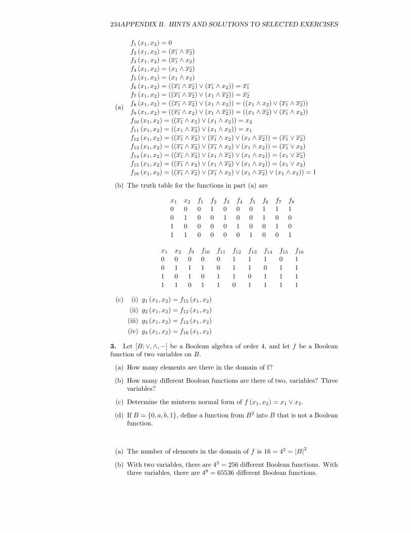
234APPENDIX B. HINTS AND SOLUTIONS TO SELECTED EXERCISES
(a)
f1 (x1, x2) = 0
f2 (x1, x2) = (x1 ∧ x2)
f3 (x1, x2) = (x1 ∧ x2)
f4 (x1, x2) = (x1 ∧ x2)
f5 (x1, x2) = (x1 ∧ x2)
f6 (x1, x2) = ((x1 ∧ x2) ∨ (x1 ∧ x2)) = x1
f7 (x1, x2) = ((x1 ∧ x2) ∨ (x1 ∧ x2)) = x2
f8 (x1, x2) = ((x1 ∧ x2) ∨ (x1 ∧ x2)) = ((x1 ∧ x2) ∨ (x1 ∧ x2))
f9 (x1, x2) = ((x1 ∧ x2) ∨ (x1 ∧ x2)) = ((x1 ∧ x2) ∨ (x1 ∧ x2))
f10 (x1, x2) = ((x1 ∧ x2) ∨ (x1 ∧ x2)) = x2
f11 (x1, x2) = ((x1 ∧ x2) ∨ (x1 ∧ x2)) = x1
f12 (x1, x2) = ((x1 ∧ x2) ∨ (x1 ∧ x2) ∨ (x1 ∧ x2)) = (x1 ∨ x2)
f13 (x1, x2) = ((x1 ∧ x2) ∨ (x1 ∧ x2) ∨ (x1 ∧ x2)) = (x1 ∨ x2)
f14 (x1, x2) = ((x1 ∧ x2) ∨ (x1 ∧ x2) ∨ (x1 ∧ x2)) = (x1 ∨ x2)
f15 (x1, x2) = ((x1 ∧ x2) ∨ (x1 ∧ x2) ∨ (x1 ∧ x2)) = (x1 ∨ x2)
f16 (x1, x2) = ((x1 ∧ x2) ∨ (x1 ∧ x2) ∨ (x1 ∧ x2) ∨ (x1 ∧ x2)) = 1
(b) The truth table for the functions in part (a) are
x1 x2 f1 f2 f3 f4 f5 f6 f7 f8
0 0 0 1 0 0 0 1 1 1
0 1 0 0 1 0 0 1 0 0
1 0 0 0 0 1 0 0 1 0
1 1 0 0 0 0 1 0 0 1
x1 x2 f9 f10 f11 f12 f13 f14 f15 f16
0 0 0 0 0 1 1 1 0 1
0 1 1 1 0 1 1 0 1 1
1 0 1 0 1 1 0 1 1 1
1 1 0 1 1 0 1 1 1 1
(c) (i) g1 (x1, x2) = f15 (x1, x2)
(ii) g2 (x1, x2) = f12 (x1, x2)
(iii) g3 (x1, x2) = f12 (x1, x2)
(iv) g4 (x1, x2) = f16 (x1, x2)
3. Let [B;∨,∧,−] be a Boolean algebra of order 4, and let f be a Booleanfunction of two variables on B.
(a) How many elements are there in the domain of f?
(b) How many different Boolean functions are there of two, variables? Threevariables?
(c) Determine the minterm normal form of f (x1, x2) = x1 ∨ x2.
(d) If B = {0, a, b, 1}, define a function from B2 into B that is not a Booleanfunction.
(a) The number of elements in the domain of f is 16 = 42 = |B|2
(b) With two variables, there are 43 = 256 different Boolean functions. Withthree variables, there are 48 = 65536 different Boolean functions.
235
(c) f (x1, x2) = (1 ∧ x1 ∧ x2) ∨ (1 ∧ x1 ∧ x2) ∨ (1 ∧ x1 ∧ x2) ∨ (0 ∧ x1 ∧ x2)
(d) Consider f : B2 → B, defined by f(0, 0) = 0, f(0, 1) = 1, f(1, 0) = a,f(1, 1) = a, and f(0, a) = b, with the images of all other pairs in B2
defined arbitrarily. This function is not a Boolean function. If we as-sume that it is Boolean function then f can be computed with a Booleanexpression M (x1, x2). This expression can be put into minterm nor-mal form: M (x1, x2) = (c1 ∧ x1 ∧ x2) ∨ (c2 ∧ x1 ∧ x2) ∨ (c3 ∧ x1 ∧ x2) ∨(c4 ∧ x1 ∧ x2)
f(0, 0) = 0⇒M(0, 0) = 0⇒ c1 = 0
f(0, 1) = 1⇒M(0, 0) = 1⇒ c2 = 1
f(1, 0) = a⇒M(0, 0) = a⇒ c3 = a
f(1, 1) = a⇒M(0, 0) = a⇒ c4 = a
Therefore, M (x1, x2) = (x1 ∧ x2) ∨ (a ∧ x1 ∧ x2) ∨ (a ∧ x1 ∧ x2) and so,using this formula, M(0, a) = (0 ∧ a) ∨ (a ∧ 0 ∧ a) ∨ (a ∧ 0 ∧ a) = a Thiscontradicts f(0, a) = b, and so f is not a Boolean function.
Exercises for Section 14.11. For each of the subsets of the indicated monoid, determine whether thesubset is a submonoid.
(a) S1 = {0, 2, 4, 6} and S2 = {1, 3, 5, 7} in [Z8;×8].
(b) {f ∈ NN : f(n) 6 n, ∀n ∈ N} and{f ∈ NN : f(1) = 2
}in the monoid
[NN; ◦].
(c) {A ⊆ Z | A is finite} and {A ⊆ Z | Ac is finite} in [P(Z);∪].
(a) S1 is not a submonoid since the identity of [Z8;×8], which is 1, is not inS1. S2 is a submonoid since 1 ∈ S2 and S2 is closed under multiplication;that is, for all a, b ∈ S2, a×8 b is in S2.
(b) The identity of NN is the identity function i : N→ N defined by i(a) = a,∀a ∈ N. If a ∈ N, i(a) = a ≤ a, thus the identity of NN is in S1. However,the image of 1 under any function in S2 is 2, and thus the identity ofNN is not in S2, so S2 is not a submonoid. The composition of any twofunctions in S1, f and g, will be a function in S1:
(f ◦ g)(n) = f(g(n)) ≤ g(n) since f is in S1
≤ n since g is in S1 ⇒ f ◦ g ∈ S1
and the two conditions of a submonoid are satisfied and S1 is a submonoidof NN.
(c) The first set is a submonoid, but the second is not since the null set hasa non-finite complement.
3. An n × n matrix of real numbers is called stochastic if and only if eachentry is nonnegative and the sum of entries in each column is 1. Prove thatthe set of stochastic matrices is a monoid over matrix multiplication.
The set of n × n real matrices is a monoid under matrix multiplication.This follows from the laws of matrix algebra in Chapter 5. To prove that the
236APPENDIX B. HINTS AND SOLUTIONS TO SELECTED EXERCISES
set of stochastic matrices is a monoid over matrix multiplication, we need onlyshow that the identity matrix is stochastic (this is obvious) and that the setof stochastic matrices is closed under matrix multiplication. Let A and B ben× n stochastic matrices.
(AB)ij =
n∑k=1
aikbkj
The sum of the jth column isn∑j=1
(AB)ij =
n∑k=1
a1kbkj +
n∑k=1
a1kbkj + · · ·+n∑k=1
ankbkj
=
n∑k=1
(a1kbkj + a1kbkj + · · ·+ ankbkj)
=
n∑k=1
bkj (a1k + a1k + · · ·+ ank)
=
n∑k=1
bkj since A is stochastic
= 1 since B is stochastic
5. Let B be a Boolean algebra and M the set of all Boolean functions onB. Let ∗ be defined on M by (f ∗ g)(a) = f(a) ∧ g(a). Prove that [M ; ∗] is amonoid. Construct the operation table of [M ; ∗] for the case of B = B2.
Let f, g, h ∈M , and a ∈ B.
((f ∗ g) ∗ h)(a) = (f ∗ g)(a) ∧ h(a)
= (f(a) ∧ g(a)) ∧ h(a)
= f(a) ∧ (g(a) ∧ h(a))
= f(a) ∧ (g ∗ h)(a)
= (f ∗ (g ∗ h))(a)
Therefore (f ∗ g) ∗ h = f ∗ (g ∗ h) and ∗ is associative.The identity for ∗ is the function u ∈M where u(a) = 1 = the “one” of B.
If a ∈ B, (f ∗ u)(a) = f(a) ∧ u(a) = f(a) ∧ 1 = f(a). Therefore f ∗ u = f .Similarly, u ∗ f = f .
There are 22 = 4 functions in M for B = B2. These four functions arenamed in the text. See Figure 14.1.4. The table for ∗ is
∗ z i t u
z z z z z
i z i z i
t z z t t
u z i t u
Exercises for Section 14.21.
(a) If a computer is being designed to operate with a character set of 350symbols, how many bits must be reserved for each character? Assumeeach character will use the same number of bits.
237
(b) Do the same for 3,500 symbols.
(a) For a character set of 350 symbols, the number of bits needed for eachcharacter is the smallest n such that 2n is greater than or equal to 350.Since 29 = 512 > 350 > 28, 9 bits are needed,
(b) 212 = 4096 > 3500 > 211; therefore, 12 bits are needed.
3. What sets of strings are defined by the following grammar?
(a) Terminal symbols: λ , 0 and 1
(b) Nonterminal symbols: S and E
(c) Starting symbol: S
(d) Production rules: S → 0S0, S → 1S1, S → E,E → λ,E → 0, E → 1
This grammar defines the set of all strings over B for which each string isa palindrome (same string if read forward or backward).5. Define the following languages over B with phrase structure grammars.Which of these languages are regular?
(a) The strings with an odd number of characters.
(b) The strings of length 4 or less.
(c) The palindromes, strings that are the same backwards as forwards.
(a) Terminal symbols: The null string, 0, and 1. Nonterminal symbols: S,E. Starting symbol: S. Production rules: S → 00S, S → 01S, S → 10S,S → 11S, S → E, E → 0, E → 1 This is a regular grammar.
(b) Terminal symbols: The null string, 0, and 1. Nonterminal symbols: S,A, B, C Starting symbol: S Production rules: S → 0A, S → 1A, S → λ, A→ 0B, A→ 1B, A→ λ, B → 0C, B → 1C, B → A, C → 0, C → 1,C → λ This is a regular grammar.
(c) See Exercise 3. This language is not regular.
7. Prove that if a language over A is recursive, then its complement is alsorecursive.
If s is in A∗ and L is recursive, we can answer the question “Is s in Lc?” bynegating the answer to “Is s in L?”9.
(a) Prove that if X1, X2, . . .is a countable sequence of countable sets, theunion of these sets,
∞∪i=1Xi is countable.
(b) Using the fact that the countable union of countable sets is countable,prove that if A is countable, then A∗ is countable.
238APPENDIX B. HINTS AND SOLUTIONS TO SELECTED EXERCISES
(a) List the elements of each set Xi in a sequence xi1, xi2, xi3 . . . . Thendraw arrows as shown below and list the elements of the union in orderestablished by this pattern: x11, x21, x12, x13, x22, x31, x41, x32, x23,x14, x15 . . .,
(b) Each of the sets A1 , A2 , A3, . . ., are countable and A∗ is the union ofthese sets; hence A∗ is countable.
Figure B.0.4: Exercise 9
Exercises for Section 14.3
1. Draw a transition diagram for the vending machine described in Exam-ple 14.3.2.
x s Z(x, s) t(x, s)
Deposit25 6 c Locked Nothing SelectDeposit25 6 c Select Return25 6 c Select
PressS Locked Nothing LockedPressS Select DispenseS LockedPressP Locked Nothing LockedPressP Select DispenseP LockedPressB Locked Nothing LockedPressB Select DispenseB Locked
239
Figure B.0.5: Vending Machine Transitions
3. What is the input set for the binary adding machine in Example 14.3.9?{000, 011, 101, 110, 111}
5. The Gray Code Decoder. The finite-state machine defined by the followingfigure has an interesting connection with the Gray Code.
Figure B.0.6: Gray Code Decoder
Given a string x = x1x2 · · ·xn ∈ Bn, we may ask where x appears in Gn.Starting in Copy state, the input string x will result in an output string z ∈ Bn,which is the binary form of the position of x in Gn. Recall that positions arenumbered from 0 to 2n − 1.
(a) In what positions (0− 31) do 10110, 00100, and 11111 appear in G5?
(b) Prove that the Gray Code Decoder always works.
(a) • Input: 10110, Output: 11011 ⇒ 10110 is in position 27
• Input: 00100, Output: 00111 ⇒ 00100 is in position 7
• Input:11111, Output: 10101 ⇒ 11111 is in position 21
(b) Let x = x1x2 . . . xn and recall that for n ≥ 1, Gn+1 =
(0Gn1Grn
), where
Grn is the reverse of Gn. To prove that the Gray Code Decoder alwaysworks, let p(n) be the proposition “Starting in Copy state, x’s output isthe position of x in Gn; and starting in Complement state, x’s output
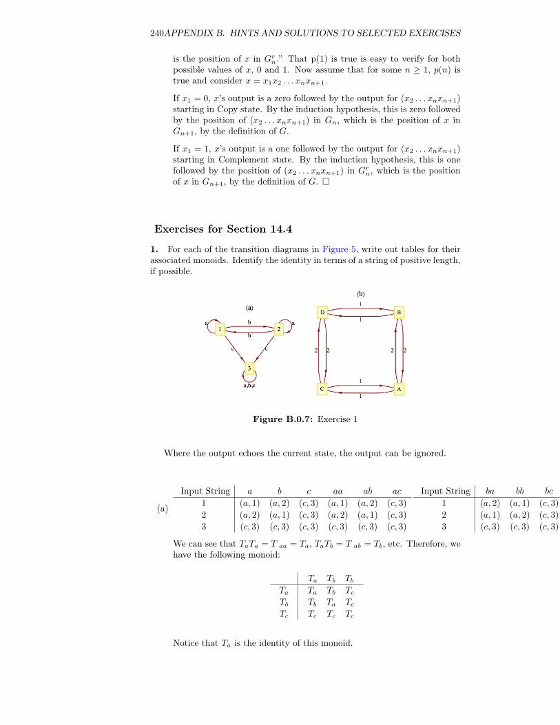
240APPENDIX B. HINTS AND SOLUTIONS TO SELECTED EXERCISES
is the position of x in Grn.” That p(1) is true is easy to verify for bothpossible values of x, 0 and 1. Now assume that for some n ≥ 1, p(n) istrue and consider x = x1x2 . . . xnxn+1.
If x1 = 0, x’s output is a zero followed by the output for (x2 . . . xnxn+1)starting in Copy state. By the induction hypothesis, this is zero followedby the position of (x2 . . . xnxn+1) in Gn, which is the position of x inGn+1, by the definition of G.
If x1 = 1, x’s output is a one followed by the output for (x2 . . . xnxn+1)starting in Complement state. By the induction hypothesis, this is onefollowed by the position of (x2 . . . xnxn+1) in Grn, which is the positionof x in Gn+1, by the definition of G. �
Exercises for Section 14.4
1. For each of the transition diagrams in Figure 5, write out tables for theirassociated monoids. Identify the identity in terms of a string of positive length,if possible.
Figure B.0.7: Exercise 1
Where the output echoes the current state, the output can be ignored.
(a)
Input String a b c aa ab ac
1 (a, 1) (a, 2) (c, 3) (a, 1) (a, 2) (c, 3)
2 (a, 2) (a, 1) (c, 3) (a, 2) (a, 1) (c, 3)
3 (c, 3) (c, 3) (c, 3) (c, 3) (c, 3) (c, 3)
Input String ba bb bc ca cb cc
1 (a, 2) (a, 1) (c, 3) (c, 3) (c, 3) (c, 3)
2 (a, 1) (a, 2) (c, 3) (c, 3) (c, 3) (c, 3)
3 (c, 3) (c, 3) (c, 3) (c, 3) (c, 3) (c, 3)
We can see that TaTa = T aa = Ta, TaTb = T ab = Tb, etc. Therefore, wehave the following monoid:
Ta Tb TbTaTbTc
Ta Tb TcTb Ta TcTc Tc Tc
Notice that Ta is the identity of this monoid.
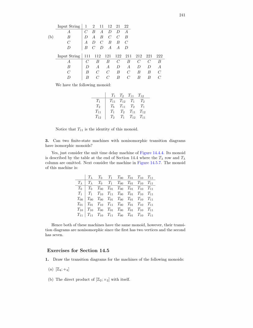
241
(b)
Input String 1 2 11 12 21 22
A C B A D D A
B D A B C C B
C A D C B B C
D B C D A A D
Input String 111 112 121 122 211 212 221 222
A C B B C B C C B
B D A A D A D D A
C B C C B C B B C
D B C C B C B B C
We have the following monoid:
T1 T2 T11 T12
T1
T2
T11
T12
T11 T12 T1 T2
Tb T11 T2 T1
T1 T2 T11 T12
T2 T1 T12 T11
Notice that T11 is the identity of this monoid.
3. Can two finite-state machines with nonisomorphic transition diagramshave isomorphic monoids?
Yes, just consider the unit time delay machine of Figure 14.4.4. Its monoidis described by the table at the end of Section 14.4 where the Tλ row and Tλcolumn are omitted. Next consider the machine in Figure 14.5.7. The monoidof this machine is:
Tλ T0 T1 T00 T01 T10 T11
Tλ Tλ T0 T1 T00 T01 T10 T11
T0 T0 T00 T01 T00 T01 T10 T11
T1 T1 T10 T11 T00 T01 T10 T11
T00 T00 T00 T01 T00 T01 T10 T11
T01 T01 T10 T11 T00 T01 T10 T11
T10 T10 T00 T01 T00 T01 T10 T11
T11 T11 T10 T11 T00 T01 T10 T11
Hence both of these machines have the same monoid, however, their transi-tion diagrams are nonisomorphic since the first has two vertices and the secondhas seven.
Exercises for Section 14.5
1. Draw the transition diagrams for the machines of the following monoids:
(a) [Z4; +4]
(b) The direct product of [Z2;×2] with itself.
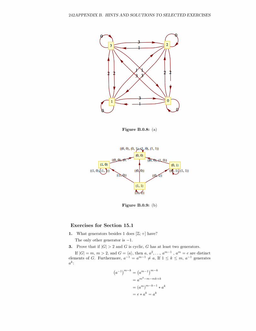
242APPENDIX B. HINTS AND SOLUTIONS TO SELECTED EXERCISES
Figure B.0.8: (a)
Figure B.0.9: (b)
Exercises for Section 15.1
1. What generators besides 1 does [Z; +] have?The only other generator is −1.
3. Prove that if |G| > 2 and G is cyclic, G has at least two generators.If |G| = m, m > 2, and G = 〈a〉, then a, a2, . . ., am−1 , am = e are distinct
elements of G. Furthermore, a−1 = am−1 6= a, If 1 ≤ k ≤ m, a−1 generatesak: (
a−1)m−k
=(am−1
)m−k= am
2−m−mk+k
= (am)m−k−1 ∗ ak
= e ∗ ak = ak
243
Similarly, if G is infinite and G = 〈a〉, then a−1 generates G.5. Which of the following groups are cyclic? Explain.
(a) [Q; +]
(b) [R+; ·]
(c) [6Z; +] where 6Z = {6n|n ∈ Z}
(d) Z× Z
(e) Z2 × Z3 × Z25
(a) No. Assume that q ∈ Q generates Q. Then 〈q〉 = {nq : n ∈ Z}. But thisgives us at most integer multiples of q, not every element in Q.
(b) No. Similar reasoning to part a.
(c) Yes. 6 is a generator of 6Z.
(d) No.
(e) Yes, (1, 1, 1) is a generator of the group.
7. How can Theorem 15.1.13 be applied to list the generators of Zn? Whatare the generators of Z25? Of Z256?
Theorem 15.1.13 implies that a generates Zn if and only if the greatestcommon divisor of n and a is 1. Therefore the list of generators of Zn are theintegers in Zn that are relatively prime to n. The generators of Z25 are all ofthe nonzero elements except 5, 10, 15, and 20. The generators of Z256 are theodd integers in Z256 since 256 is 28.9.
(a) Illustrate how the fast adder can be used to add the numbers 21, 5, 7,and 15 using the isomorphism between Z77 and Z7 × Z11.
(b) If the same isomorphism is used to add the numbers 25, 26, and 40, whatwould the result be, why would it be incorrect, and how would the answerdiffer from the answer in part a?
(a) θ : Z77 → Z7 × Z11 maps the given integers as follows:
21 → (0, 10)
5 → (5, 5)
7 → (0, 7)
15 → (1, 4)
sum = 48 ← (6, 4) = sum
The final sum, 48, is obtained by using the facts that θ−1(1, 0) = 22 andθ−1(0, 1) = 56
θ−1(6, 4) = 6×77 θ−1(1, 0) + 4×77 θ
−1(0, 1)
= 6×77 22 +77 4×77 56
= 55 +77 70
= 48
.
244APPENDIX B. HINTS AND SOLUTIONS TO SELECTED EXERCISES
(b) Using the same isomorphism:
25 → (4, 3)
26 → (5, 4)
40 → (5, 7)
sum = (0, 3)
theta−1(0, 3) = 3×77 θ−1(0, 1)
= 3×77 56
= 14
.
The actual sum is 91. Our result is incorrect, since 91 is not in Z77.Notice that 91 and 14 differ by 77. Any error that we get using thistechnique will be a multiple of 77.
Exercises for Section 15.21. Consider Z10 and the subsets of Z10, {0, 1, 2, 3, 4} and {5, 6, 7, 8, 9}. Why isthe operation induced on these subsets by modulo 10 addition not well defined?
An example of a valid correct answer: Call the subsets A and B respectively.If we choose 0 ∈ A and 5 ∈ B we get 0 +10 5 = 5 ∈ B. On the other hand, ifwe choose 3 ∈ A and 8 ∈ B, we get 3 +10 8 = 1 ∈ A. Therefore, the inducedoperation is not well defined on {A,B}.3. For each group and subgroup, what is G/H isomorphic to?
(a) G = Z4 × Z2 and H = 〈(2, 0)〉. Compare to Example 15.2.16.
(b) G = [C; +] and H = R.
(c) G = Z20 and H = 〈8〉.
(a) The four distinct cosets in G/H are H = {(0, 0), (2, 0)}, (1, 0) + H ={(1, 0), (3, 0)}, (0, 1)+H = {(0, 1), (2, 1)}, and (1, 1)+H = {(1, 1), (3, 1)}.None of these cosets generates G/H; therefore G/H is not cyclic. HenceG/H must be isomorphic to Z2 × Z2.
(b) The factor group is isomorphic to [R; +]. Each coset of R is a line inthe complex plane that is parallel to the x-axis: τ : C/R → R, whereT ({a+ bi | a ∈ R}) = b is an isomorphism.
(c) 〈8〉 = {0, 4, 8, 12, 16}⇒ |Z20/〈8〉| = 4. The four cosets are: 0, 1, 2, and3. 1 generates all four cosets. The factor group is isomorphic to [Z4; +4]because 1 is a generator.
5. Assume that G is a group, H ≤ G, and a, b ∈ G. Prove that a ∗H = b ∗Hif and only if b−1 ∗ a ∈ H.
a ∗H = b ∗H ⇔ a ∈ bH⇔ a = b ∗ h for some h ∈ H⇔ b−1 ∗ a = h for some h ∈ H⇔ b−1 ∗ a ∈ H
245
Exercises for Section 15.3
1. Given f =
(1 2 3 4
2 1 4 3
), g =
(1 2 3 4
2 3 4 1
), and h =
(1 2 3 4
3 2 4 1
),
compute
(a) f ◦ g
(b) g ◦ h
(c) (f ◦ g) ◦ h
(d) f ◦ (g ◦ h)
(e) h−1
(f) h−1g ◦ h
(g) f−1
(a)(
1 2 3 4
1 4 3 2
)
(b)(
1 2 3 4
4 3 1 2
)
(c)(
1 2 3 4
3 4 2 1
)
(d)(
1 2 3 4
3 4 2 1
)
(e)(
1 2 3 4
4 2 1 3
)
(f)(
1 2 3 4
3 1 4 2
)
(g)(
1 2 3 4
2 1 4 3
)3. Do the left cosets of A3 = {i, r1, r2} over S3 form a group under theinduced operation on left cosets of A3? What about the left cosets of 〈f1〉?
S3/A3 is a group of order two. The operation on left cosets of H = 〈f1〉 isnot well defined and so a group cannot be formed from left cosets of H.5.
(a) Complete the list of elements of D4 and write out a table for the groupin its realization as symmetries.
(b) List the subgroups of D4 in a lattice diagram. Are they all cyclic? Towhat simpler groups are the subgroups of D4 isomorphic?
D4 ={i, r, r2, r3, f1, f2, f3, f4
}Where i is the identity function, r =
(1 2 3 4
2 3 4 1
),
and
f1 =
(1 2 3 4
4 3 2 1
)f2 =
(1 2 3 4
2 1 4 3
)f3 =
(1 2 3 4
3 2 1 4
)f4 =
(1 2 3 4
1 4 3 2
)The operation table for the group is
◦ i r r2 r3 f1 f2 f3 f4
i
r
r2
r3
f1
f2
f3
f4
i r r2 r3 f1 f2 f3 f4
r r2 r3 i f4 f3 f1 f2
r2 r3 i r f2 f1 f4 f3
r3 i r r2 f3 f4 f2 f1
f1 f3 f2 f4 i r2 � r3
f2 f4 f1 f3 r2 i r3 r
f3 f2 f4 f1 r3 r i r2
f4 f1 f3 f2 r r3 r2 i
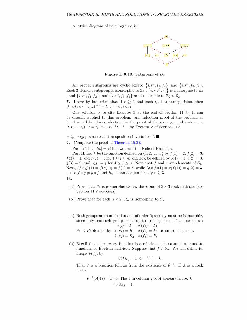
246APPENDIX B. HINTS AND SOLUTIONS TO SELECTED EXERCISES
A lattice diagram of its subgroups is
Figure B.0.10: Subgroups of D4
All proper subgroups are cyclic except{i, r2, f1, f2
}and
{i, r2, f3, f4
}.
Each 2-element subgroup is isomorphic to Z2 ;{i, r, r2, r3
}is isomorphic to Z4
; and{i, r2, f1, f2
}and
{i, r2, f3, f4
}are isomorphic to Z2 × Z2.
7. Prove by induction that if r ≥ 1 and each ti, is a transposition, then(t1 ◦ t2 ◦ · · · ◦ tr)−1 = tr ◦ · · · ◦ t2 ◦ t1
One solution is to cite Exercise 3 at the end of Section 11.3. It canbe directly applied to this problem. An induction proof of the problem athand would be almost identical to the proof of the more general statement.(t1t2 · · · tr)−1 = tr
−1 · · · t2−1t1−1 by Exercise 3 of Section 11.3
= tr · · · t2t1 since each transposition inverts itself. �9. Complete the proof of Theorem 15.3.9.
Part I: That |Sk| = k! follows from the Rule of Products.Part II: Let f be the function defined on {1, 2, ..., n} by f(1) = 2, f(2) = 3,
f(3) = 1, and f(j) = j for 4 ≤ j ≤ n; and let g be defined by g(1) = 1, g(2) = 3,g(3) = 2, and g(j) = j for 4 ≤ j ≤ n. Note that f and g are elements of Sn.Next, (f ◦ g)(1) = f(g(1)) = f(1) = 2, while (g ◦ f)(1) = g(f(1)) = g(2) = 3,hence f ◦ g 6= g ◦ f and Sn is non-abelian for any n ≥ 3.13.
(a) Prove that S3 is isomorphic to R3, the group of 3× 3 rook matrices (seeSection 11.2 exercises).
(b) Prove that for each n ≥ 2, Rn is isomorphic to Sn.
(a) Both groups are non-abelian and of order 6; so they must be isomorphic,since only one such group exists up to isomorphism. The function θ :
S3 → R3 defined byθ(i) = I θ (f1) = F1
θ (r1) = R1 θ (f2) = F2
θ (r2) = R2 θ (f3) = F3
is an isomorphism,
(b) Recall that since every function is a relation, it is natural to translatefunctions to Boolean matrices. Suppose that f ∈ Sn. We will define itsimage, θ(f), by
θ(f)kj = 1 ⇔ f(j) = k
That θ is a bijection follows from the existence of θ−1. If A is a rookmatrix,
θ−1(A)(j) = k ⇔ The 1 in column j of A appears in row k
⇔ Akj = 1
247
For f, g ∈ Sn,
θ(f ◦ g)kj = 1⇔ (f ◦ g)(j) = k
⇔ ∃l such that g(j) = l and f(l) = k
⇔ ∃l such that θ(g)lj = 1 and θ(f)kl = 1
⇔ (θ(f)θ(g))kj = 1
Therefore, θ is an isomorphism.
Exercises for Section 15.4
1. Which of the following functions are homomorphisms? What are the ker-nels of those functions that are homomorphisms?
(a) θ1 : R∗ → R+ defined by θ1(a) = |a|.
(b) θ2 : Z5 → Z2 where θ2(n) =
{0 if n is even1 if n is odd
.
(c) θ3 : R× R→ R, where θ3(a, b) = a+ b.
(d) θ4 : S4 → S4 defined by θ4(f) = f ◦ f = f2.
(a) Yes, the kernel is {1,−1}
(b) No, since θ2 (2 +5 4) = θ2(1) = 1, but θ2(2) +2 θ2(4) = 0 +2 0 = 0
A follow-up might be to ask what happens if 5 is replaced with someother positive integer in this part.
(c) Yes, the kernel is {(a,−a)|a ∈ R}
(d) No. A counterexample, among many, would be to consider the two trans-positions t1 = (1, 3) and t2 = (1, 2). Compare θ4(t1◦t2) and θ4(t1)◦θ4(t2).
3. Show that D4 has one proper normal subgroup, but that 〈(1, 4)(2, 3)〉 isnot normal.
〈r〉 ={i, r, r2, r3
}is a normal subgroup of D4. To see you could use the
table given in the solution of Exercise 15.3.5 of Section 15.3 and verify thata−1ha ∈ 〈r〉 for all a ∈ D4 and h ∈ 〈r〉. A more efficient approach is to provethe general theorem that if H is a subgroup G with exactly two distinct leftcosets, than H is normal. 〈f1〉 is not a normal subgroup of D4. 〈f1〉 = {i, f1}and if we choose a = r and h = f1 then a−1ha = r3f1r = f2 /∈ 〈f1〉5. Define the two functions α : Z2
3 → Z24 and β : Z2
4 → Z2 by α (a1, a2, a3) =(a1, a2, a3, a1 +2 a2 +2 a3), and β (b1, b2, b3, b4) = b1 + b2 + b3 + b4 Describe thefunction β ◦ α. Is it a homomorphism?
(β ◦ α) (a1, a2, a3) = 0 and so β ◦ α is the trivial homomorphism, but ahomomorphism nevertheless.
7. Prove that if G is an abelian group, then q(x) = x2 defines a homomor-phism from G into G. Is q ever an isomorphism?
248APPENDIX B. HINTS AND SOLUTIONS TO SELECTED EXERCISES
Let x, y ∈ G.
q(x ∗ y) = (x ∗ y)2
= x ∗ y ∗ x ∗ y= x ∗ x ∗ y ∗ y since G is abelian
= x2 ∗ y2
= q(x) ∗ q(y)
Hence, q is a homomorphism. In order for q to be an isomorphism, it must bethe case that no element other than the identity is its own inverse.
x ∈ Ker(q)⇔ q(x) = e
⇔ x ∗ x = e
⇔ x−1 = x
9. Prove that if θ : G → G′ is a homomorphism, and H ′ ≤ θ(G), thenθ−1(H ′) = {a ∈ G|θ(a) ∈ H ′} ≤ G.
Proof: Recall that the inverse image of H ′ under θ is θ−1(H ′) = {g ∈G|θ(g) ∈ H ′}.
Closure: Let g1, g2 ∈ θ−1(H ′), then θ (g1) , θ (g2) ∈ H ′. Since H ′ is asubgroup of G′,
θ (g1) � θ (g2) = θ (g1 ∗ g2) ∈ H ′ ⇒ g1 ∗ g2 ∈ θ−1(H ′)
Identity: By Theorem 15.4.14(a), e ∈ θ−1(H ′).Inverse: Let a ∈ θ−1(H ′) . Then θ(a) ∈ H ′ and by Theorem 15.4.14(b),
θ(a)−1 = θ(a−1
)∈ H ′ and so a−1 ∈ θ−1(H ′).
Exercises for Section 15.51. If the error-detecting code is being used, how would you act on the follow-ing received blocks?
(a) (1, 0, 1, 1)
(b) (1, 1, 1, 1)
(c) (0, 0, 0, 0)
(a) Error detected, since an odd number of 1’s was received; ask for retrans-mission.
(b) No error detected; accept this block.
(c) No error detected; accept this block.
3. If the error-correcting code is being used, how would you decode the fol-lowing blocks? Expect a problem with one of these. Why?
(a) (1, 0, 0, 0, 1, 1)
(b) (1, 0, 1, 0, 1, 1)
(c) (0, 1, 1, 1, 1, 0)
249
(d) (0, 0, 0, 1, 1, 0)
(a) Syndrome = (1, 0, 1). Corrected message is (1, 1, 0).
(b) Syndrome = (1, 1, 0). Corrected message is (0, 0, 1).
(c) Syndrome = (0, 0, 0). No error, message is (0, 1, 1).
(d) Syndrome = (1, 1, 0). Corrected message is (1, 0, 0).
(e) Syndrome = (1, 1, 1). This syndrome occurs only if two bits have beenswitched. No reliable correction is possible.
5. Consider the linear code defined by the generator matrix
G =
(1 0 1 0
0 1 1 1
)
(a) What size blocks does this code encode and what is the length of thecode words?
(b) What are the code words for this code?
(c) With this code, can you detect single bit errors? Can you correct all,some, or no single bit errors?
Let G be the 9×10 matrix obtained by augmenting the 9×9 identity matrixwith a column of ones. The function e : Z2
9 → Z210 defined by e(a) = aG will
allow us to detect single errors, since e(a) will always have an even number ofones.
Exercises for Section 16.11. Review the definition of rings to show that the following are rings. Theoperations involved are the usual operations defined on the sets. Which ofthese rings are commutative? Which are rings with unity? For the rings withunity, determine the unity and all units.
(a) [Z; +, ·]
(b) [C; +, ·]
(c) [Q; +, ·]
(d) [M2×2(R); +, ·]
(e) [Z2; +2,×2]
All but ring d are commutative. All of the rings have a unity element. Thenumber 1 is the unity for all of the rings except d. The unity for M2×2(R) isthe two by two identity matrix. The units are as follows:
(a) {1,−1}
(b) C∗
(c) Q∗
(d) {A |A11A22 −A12A21 6= 0}
(e) {1}
250APPENDIX B. HINTS AND SOLUTIONS TO SELECTED EXERCISES
3. Show that the following pairs of rings are not isomorphic:
(a) [Z; +, ·] and [M2×2(Z); +, ·]
(b) [3Z; +, ·] and [4Z; +, ·].
(a) Consider commutativity
(b) Solve x2 = 3x in both rings.
5.
(a) Show that 3Z is a subring of the ring [Z; +, ·]
(b) Find all subrings of Z8.
(c) Find all subrings of Z2 × Z2.
(a) We already know that 3Z is a subgroup of the group Z. We need onlyshow that 3Z is closed with respect to multiplication. Let 3m, 3n ∈ 3Z.(3m)(3n) = 3(3mn) ∈ 3Z, since 3mn ∈ Z.
(b) The proper subrings are {0, 2, 4, 6} and {0, 4}; while {0} and Z8 areimproper subrings.
(c) The proper subrings are {00, 01}, {00, 10}, and {00, 11}: while {00} andZ2 × Z2 are improper subrings.
7.
(a) Determine all solutions of the equation x2−5x+6 = 0 in Z. Can there beany more than two solutions to this equation (or any quadratic equation)in Z?
(b) Find all solutions of the equation in part a in Z12. Why are there morethan two solutions?
(a) The left-hand side of the equation factors into the product (x−2)(x−3).Since Z is an integral domain, x = 2 and x = 3 are the only possiblesolutions.
(b) Over Z12, 2, 3, 6, and 11 are solutions. Although the equation factorsinto (x− 2)(x− 3), this product can be zero without making x either 2or 3. For example. If x = 6 we get (6 − 2) ×12 (6 − 3) = 4 ×12 3 = 0.Notice that 4 and 3 are zero divisors.
9. The relation “is isomorphic to” on rings is an equivalence relation. Explainthe meaning of this statement.
Let R1, R2, and R3 be any rings, then
(a) R1 is isomorphic to R1 and so “is isomorphic to” is a reflexive relation onrings.
(b) R1 is isomorphic to R2 ⇒ R2 is isomorphic to R1, and so “is isomorphicto” is a symmetric relation on rings,
251
(c) R1 is isomorphic to R2, and R2 is isomorphic to R3 implies that R1 isisomorphic to R3, and so “is isomorphic to” is a transitive relation onrings.
We haven’t proven these properties here, just stated them. The combinationof these observations implies that “is isomorphic to” is an equivalence relationon rings.11.
(a) Prove that the ring Z2 × Z3 is commutative and has unity.
(b) Determine all zero divisors for the ring Z2 × Z3.
(c) Give another example illustrating the fact that the product of two integraldomains may not be an integral domain. Is there an example where theproduct is an integral domain?
(a) Commutativity is clear from examination of a multiplication table forZ2×Z3. More generally, we could prove a theorem that the direct productof two or more commutative rings is commutative. (1, 1) is the unity ofZ2 × Z3.
(b) {(m,n)|m = 0 or n = 0, (m,n) 6= (0, 0)}
(c) Another example is Z × Z. You never get an integral domain in thissituation. By the definition an integral domain D must contain a “zero”so we always have (1, 0) · (0, 1) = (0, 0) in D ×D.
13.
(a) For any ring [R; +, ·], expand (a+ b)(c+ d) for a, b, c, d ∈ R.
(b) If R is commutative, prove that (a+ b)2 = a2 + 2ab+ b2 for all a, b ∈ R.
(a) (a+ b)(c+ d) = (a+ b)c+ (a+ b)d = ac+ bc+ ad+ bd
(b)
(a+ b)(a+ b) = aa+ ba+ ab+ bb by part a= aa+ ab+ ab+ bb since R is commutative
= a2 + 2ab+ b2.
Exercises for Section 16.25. Determine all values x from the given field that satisfy the given equation:
(a) x+ 1 = −1 in Z2 , Z3 and Z5
(b) 2x+ 1 = 2 in Z3 and Z5
(c) 3x+ 1 = 2 Z5
252APPENDIX B. HINTS AND SOLUTIONS TO SELECTED EXERCISES
(a) 0 in Z2, 1 in Z3, 3 in Z5
(b) 2 in Z3, 3 in Z5
(c) 2 in Z5
7. Determine all solutions to the following equations over Z2. That is, findall elements of Z2 that satisfy the equations.
(a) x2 + x = 0
(b) x2 + 1 = 0
(c) x3 + x2 + x+ 1 = 0
(d) x3 + x+ 1 = 0
(a) 0 and 1 (b) 1 (c) 1 (d) none
Exercises for Section 16.31. Let f(x) = 1 + x and g(x) = 1 + x+ x2. Compute the following sums andproducts in the indicated rings.
(a) f(x) + g(x) and f(x) · g(x) in Z[x]
(b) f(x) + g(x) and f(x) · g(x) in Z2[x]
(c) (f(x) · g(x)) · f(x) in Q[x]
(d) (f(x) · g(x)) · f(x) in Z2[x]
(e) f(x) · f(x) + f(x) · g(x) in Z2[x]
(a) f(x) + g(x) = 2 + 2x+ x2 , f(x) · g(x) = 1 + 2x+ 2x2 + x3
(b) f(x) + g(x) = x2, f(x) · g(x) = 1 + x3
(c) 1 + 3x+ 4x2 + 3x3 + x4
(d) 1 + x+ x3 + x4
(e) x2 + x3
3. Prove that:
(a) The ring R is a subring of the ring R[x].
(b) The ring Z[x] is a subring of the Q[x].
(c) The ring Q[x] is a subring of the ring R[x].
(a) If a, b ∈ R, a − b and ab are in R since R is a ring in its own right.Therefore, R is a subring of R[x]. The proofs of parts b and c are similar.
5. Determine which of the following are reducible over Z2. Explain.
(a) f(x) = x3 + 1
253
(b) g(x) = x3 + x2 + x.
(c) h(x) = x3 + x2 + 1.
(d) k(x) = x4 + x2 + 1. (Be careful.)
(a) Reducible, (x+ 1)(x2 + x+ 1
)(b) Reducible, x
(x2 + x+ 1
)(c) Irreducible. If you could factor this polynomial, one factor would be
either x or x+ 1, which would give you a root of 0 or 1, respectively. Bysubstitution of 0 and 1 into this polynomial, it clearly has no roots.
(d) Reducible, (x+ 1)4
7. Give an example of the contention made in the last paragraph of thissection.
We illustrate this property of polynomials by showing that it is not truefor a nonprime polynomial in Z2[x]. Suppose that p(x) = x2 + 1, which canbe reduced to (x+ 1)2 , a(x) = x2 + x, and b(x) = x3 + x2. Since a(x)b(x) =x5 + x3 = x3
(x2 + 1
), p(x)|a(x)b(x). However, p(x) is not a factor of either
a(x) or b(x).9. Show that x2 − 3 is irreducible over Q but reducible over the field of realnumbers.
The only possible proper factors of x2 − 3 are(x−√
3)and
(x+√
3),
which are not in Q[x] but are in R[x].11. Prove Theorem 16.3.13, the Division Property for Polynomials
For n ≥ 0, let S(n) be the proposition: For all g(x) 6= 0 and f(x) withdeg f(x) = n, there exist unique polynomials q(x) and r(x) such that f(x) =g(x)q(x) + r(x), and either r(x) = 0 or deg r(x) < deg g(x).
Basis: S(0) is true, for if f(x) has degree 0, it is a nonzero constant,f(x) = c 6= 0, and so either f(x) = g(x) · 0 + c if g(x) is not a constant, orf(x) = g(x)g(x)−1 + 0 if g(x) is also a constant.
Induction: Assume that for some n ≥ 0, S(k) is true for all k ≤ n, If f(x)has degree n + 1, then there are two cases to consider. If deg g(x) > n + 1,f(x) = g(x) ·0+f(x), and we are done. Otherwise, if deg g(x) = m ≤ n+1, weperform long division as follows, where LDT’s stand for terms of lower degreethan n+ 1.
fn+1 · gm−1xn+1−m
gmxm + LDT′s )fn+1xn+1 + LDT′s
fn+1xn+1 + LDT′s
h(x)
Therefore,
h(x) = f(x)−(fn+1 · gm−1xn+1−m) g(x)⇒ f(x) =
(fn+1 · gm−1xn+1−m) g(x)+h(x)
Since deg h(x) is less than n+1, we can apply the induction hypothesis: h(x) =g(x)q(x) + r(x) with deg r(x) < deg g(x).
Therefore,
f(x) = g(x)(fn+1 · gm−1xn+1−m + q(x)
)+ r(x)
254APPENDIX B. HINTS AND SOLUTIONS TO SELECTED EXERCISES
with deg r(x) < deg g(x). This establishes the existence of a quotient andremainder. The uniqueness of q(x) and r(x) as stated in the theorem is provenas follows: if f(x) is also equal to g(x)q(x) + r(x) with deg r(x) < deg g(x),then
g(x)q(x) + r(x) = g(x)q(x) + r(x)⇒ g(x) (q(x)− q(x)) = r(x)− r(x)
Since deg r(x)− r(x) < deg g(x), the degree of both sides of the last equationis less than deg g(x). Therefore, it must be that q(x)−q(x) = 0, or q(x) = q(x)And so r(x) = r(x).
Exercises for Section 16.4
1.
(a) Use the definition of a field to show that Q(√
2) is a field.
(b) Use the definition of vector space to show that Q(√
2)is a vector space
over Q.
(c) Prove that{
1,√
2}is a basis for the vector space Q
(√2)over Q, and,
therefore, the dimension of Q(√
2) over Q is 2.
If a0 + a1
√2 ∈ Q
[√2]is nonzero, then it has a multiplicative inverse:
1
a0 + a1
√2
=1
a0 + a1
√2
a0 − a1
√2
a0 − a1
√2
=a0 − a1
√2
a02 − 2a1
2
=a0
a02 − 2a1
2− a1
a02 − 2a1
2
√2
The denominator, a02− 2a1
2, is nonzero since√
2 is irrational. Since a0a02−2a12
and −a1a02−2a12 are both rational numbers, a0 + a1
√2 is a unit of Q
[√2]. The
field containing Q[√
2]is denoted Q
(√2)and so Q
(√2)
= Q[√
2]
3. Determine the splitting field of x4 − 5x2 + 6 over Q.x4 − 5x2 + 6 = (x2 − 2)(x2 − 3) has zeros ±
√2 and ±
√3.
Q(√
2) = {a+ b√
2 | a, b ∈ Q} contains the zeros ±√
2 but does not contain±√
3, since neither are expressible in the form a+ b√
2. If we consider the set{c+ d
√3 | c, d ∈ Q(
√2)}, then this field contains ±
√3 as well as ±
√2, and is
denoted Q(√
2)(√
3) = Q(√
2,√
3). Taking into account the form of c and d inthe description above, we can expand to
Q(√
2,√
3) = {b0 + b1√
2 + b2√
3 + b3√
6 | bi ∈ Q}
5.
(a) Show that x3 + x+ 1 is irreducible over Z2.
(b) Determine the splitting field of x3 + x+ 1 over Z2.
(c) By Theorem 16.2.10, you have described all fields of order 23.
255
(a) f(x) = x3 + x + 1 is reducible if and only if it has a factor of the formx − a. By Theorem 16.3.14, x − a is a factor if and only if a is a zero.Neither 0 nor 1 is a zero of f(x) over Z2.
(b) Since f(x) is irreducible over Z2, all zeros of f(x) must lie in an extensionfield of Z2 . Let c be a zero of f(x). Z2(c) can be described severaldifferent ways. One way is to note that since c ∈ Z2(c), cn ∈ Z2(c) forall n. Therefore, Z2(c) includes 0, c, c2, c3, . . .. But c3 = c + 1 sincef(c) = 0. Furthermore, c4 = c2 + c, c5 = c2 + c + 1, c6 = c2 + 1, andc7 = 1. Higher powers of c repeat preceding powers. Therefore,
Z2(c) ={
0, 1, c, c2, c+ 1, c2 + 1, c2 + c+ 1, c2 + c}
={a0 + a1c+ a2c
2 | ai ∈ Z2
}The three zeros of f(x) are c, c2 and c2 + c.
f(x) = (x+ c)(x+ c2
) (x+ c2 + c
)(c) Cite Theorem Theorem 16.2.10, part 3.
Exercises for Section 16.5
5.
(a) Determine the inverse of h(x) =∑∞i=0 2ixi in Q[[x]].
(b) Use the procedures in Chapter 8 to find a rational generating functionfor h(x) in part a. Find the multiplicative inverse of this function.
(a)b0 = 1
b1 = (−1)(2 · 1) = −2
b2 = (−1)(2 · (−2) + 4 · 1) = 0
b3 = (−1)(2 · 0 + 4 · (−2) + 8 · 1) = 0
All other terms are zero. Hence, f(x)−1 = 1− 2x
(b)
f(x) = 1 + 2x+ 22x2 + 23x3 + · · ·= (2x)0 + (2x)1 + (2x)2 + (2x)3 + · · ·
=1
1− 2x
The last step follows from the formula for the sum of a geometric series.
7. Write as an extended power series:
(a)(x4 − x5
)−1
(b)(x2 − 2x3 + x4
)−1
256APPENDIX B. HINTS AND SOLUTIONS TO SELECTED EXERCISES
(a) (x4 − x5
)−1= (x4(1− x))−1
= x−4 1
1− x
= x−4
( ∞∑k=0
xk
)
=
∞∑k=−4
xk
.
(b) (x4 − 2x3 + x2
)−1=(x2(x2 − 2x+ 1
))−1
= x−2(1− 2x+ x2
)−1
= x−2
( ∞∑k=0
(k + 1)xk
)
=
∞∑k=−2
(k + 2)xk
.
Exercises for Part 1 of the Algorithms Appendix2. What is wrong with this algorithm?
Input: a and b, integersOutput: the value of c will be a - b(1) c = 0(2) While a > b:
(2.1) a := a - l(2.2) c := c + l
Listing B.0.11
The algorithm only works when a > b.
Exercises for Part 2 of the Algorithms Appendix2. Verify the correctness of the following algorithm to compute the greatestcommon divisor of two integers that are not both zero.
def gcd(a,b):r0=ar1=bwhile r1 !=0:
t= r0 % r1r0=r1r1=t
return r0
gcd (1001 ,154) #test
The invariant of this algorithm is gcd(r0, r1) = gcd(a, b).
Appendix C
Notation
The following table defines the notation used in this book. Page numbers orreferences refer to the first appearance of each symbol.
Symbol Description Page
a ≡m b a is congruent to b modulo m 12∗ generic symbol for a binary operation 21string1 + string2 The concatenation of string1 and string2 24[G; ∗] a group with elements G and binary operation
∗26
gcd(a, b) the greatest common divisor of a and b 34a+n b the mod n sum of a and b 38a×n b the mod n product of a and b 38Zn The Additive Group of Integer Modulo n 38Un The Multipicative Group of Integer Modulo n 38W ≤ V W is a subsystem of V 41〈a〉 the cyclic subgroup generated by a 44ord(n) Order of a 44V1 × V2 × · · · × Vn The direct product of algebraic structures
V1, V2, . . . , Vn
46
G1∼= G2 G1 is isomorphic to G2 55
74dim(V ) The dimension of vector space V 77000 least element in a poset 99111 greatest element in a poset 99Dn the set of divisors of integer n 99a ∨ b the join, or least upper bound of a and b 101a ∧ b the meet, or greatest lower bound of a and b 101[L;∨,∧] A lattice with domain having meet and join op-
erations102
a The complement of lattice element a 104[B;∨,∧, ¯ ] a boolean algebra with operations disjunction,
conjuction and complementation105
106Mδ1δ2···δk the minterm generated by x1, x2, . . . , xk, where
yi = xi if δi = 1 and yi = xi if δi = 0113
A∗ The set of all strings over an alphabet A 120(Continued on next page)
257
258 APPENDIX C. NOTATION
Symbol Description Page
An The set of all strings of length n) over an al-phabet A
120
λ The empty string 120s1 + s2 The concatenation of strings s1 and s2 121L(G) Language created by phrase structure grammar
G123
(S,X,Z,w, t) A finite-state machine with states S, input al-phabet X, output alphabet X, and outputfunction w and next-state function t
127
m(M) The machine of monoid M 135139
a ∗H,H ∗ a the left and right cosets generated by a 146G/H The factor group G mod H. 150SA The group of permutations of the set A 152Sn The group of permutatations on a set with n
elements152
An The Alternating Group 155H / G H is a normal subgroup of G 162kerθ the kernel of homomorphism θ 164[R; +, ·] a ring with domain R and operations + and · 173U(R) the set of units of a ring R 175
176178
D a generic integral domain 179degf(x) the degree of polynomial f(x) 185R[x] the set of all polynomials in x over R 185R[[x]] the set of all powers series in R 195x, x pre and post values of a variable x 206
References
Many of the references listed here were used in preparing the original 1980’sversion of this book. In most cases, the mathematics that they contain is stillworth reading for further background. Many can be found online, in universitylibraries or used bookstores. A few references more current references have beenadded.
[1] Allenby, R.B.J.T, Rings, Fields and Groups, Edward Arnold, 1983.
[2] Appel, K., and W. Haken, Every Planar Map Is 4-colorable, Bull, Am.Math. Soc. 82 (1976): 711-12.
[3] Arbib, M. A., A. J. Kfoury, and R. N. Moll, A Basis for TheoreticalComputer Science, New York: Springer-Verlag, 1981.
[4] Austin, A. Keith, An Elementary Approach to NP-Completeness Amer-ican Math. Monthly 90 (1983): 398-99.
[5] Beardwood, J., J. H. Halton, and J. M. Hammersley, The Shortest PathThrough Many Points Proc. Cambridge Phil. Soc. 55 (1959): 299-327.
[6] Ben-Ari, M, Principles of Concurrent Programming, Englewood Cliffs,NJ: Prentice-Hall, 1982.
[7] Berge, C, The Theory of Graphs and Its Applications, New York: Wiley,1962.
[8] Bogart, Kenneth P, Combinatorics Through Guided Discovery, 2005.This book may be freely downloaded and redestributed under the termsof the GNU Free Documentation License (FDL), as published by the FreeSoftware Foundation.
[9] Bronson, Richard, Matrix Methods, New York: Academic Press, 1969.
[10] Busacker, Robert G., and Thomas L. Saaty, Finite Graphs and Networks,New York: McGraw-Hill, 1965.
[11] Connell, Ian, Modern Algebra, A Constructive Introduction, New York:North-Holland, 1982.
[12] Denning, Peter J., Jack B. Dennis, and Joseph L. Qualitz, Machines,Languages, and Computation, Englewood Cliffs, NJ: Prentice-Hall, 1978.
[13] Denning, Peter J, Multigrids and Hypercubes. American Scientist 75(1987): 234-238.
[14] Dornhoff, L. L., and F. E. Hohn, Applied Modern Algebra, New York:Macmillan, 1978.
[15] Even, S, Graph Algorithms, Potomac, MD: Computer Science Press,1979.
[16] Fisher, J. L, Application-Oriented Algebra, New York: Harper and Row,1977.
259
260 APPENDIX C. NOTATION
[17] Ford, L. R., Jr., and D. R. Fulkerson, Flows in Networks, Princeton, NJ:Princeton Univesity Press, 1962.
[18] Fraleigh, John B, A First Course in Abstract Algebra, 3rd ed. Reading,MA: Addison-Wesley, 1982.
[19] Gallian, Joseph A, Contemporary Abstract Algebra, D.C. Heath, 1986.
[20] Gallian, Joseph A, Group Theory and the Design of a Letter-Facing Ma-chine, American Math. Monthly 84 (1977): 285-287.
[21] Hamming, R. W, Coding and Information Theory, Englewood Cliffs, NJ:Prentice-Hall, 1980.
[22] Hill, F. J., and G. R. Peterson, Switching Theory and Logical Design,2nd ed. New York: Wiley, 1974.
[23] Hofstadter, D. R, Godel, Escher, Bach: An Eternal Golden Braid, NewYork: Basic Books, 1979.
[24] Hohn, F. E, Applied Boolean Algebra, 2nd ed. New York: Macmillan,1966.
[25] Hopcroft, J. E., and J. D. Ullman, Formal Languages and Their Relationto Automata, Reading, MA: Addison-Wesley, 1969.
[26] Hu, T. C, Combinatorial Algorithms, Reading, MA: Addison-Wesley,1982.
[27] Knuth, D. E, The Art of Computer Programming. Vol. 1, FundamentalAlgorithms, 2nd ed. Reading, MA: Addison-Wesley, 1973.
[28] Knuth, D. E, The Art of Computer Programming. Vol. 2, SeminumericalAlgorithms, 2nd ed., Reading, MA: Addison-Wesley, 1981.
[29] Knuth, D. E, The Art of Computer Programming. Vol. 3, Sorting andSearching, Reading, MA: Addison-Wesley, 1973.
[30] Knuth, D. E, The Art of Computer Programming. Vol. 4A, Combina-torial Algorithms, Part 1, Upper Saddle River, New Jersey: Addison-Wesley, 2011.https://www-cs-faculty.stanford.edu/ knuth/taocp.html
[31] Kulisch, U. W., and Miranker, W. L, Computer Arithmetic in Theoryand Practice, New York: Academic Press, 1981.
[32] Lipson, J. D, Elements of Algebra and Algebraic Computing, Reading,MA: Addison-Wesley, 1981.
[33] Liu, C. L, Elements of Discrete Mathematics, New York: McGraw-Hill,1977.
[34] O’Donnell, Analysis of Boolean Functions.A book about Fourier analysis of boolean functions that is being devel-oped online in a blog.
[35] Ore, O, Graphs and Their Uses, New York: Random House, 1963.
[36] Parry, R. T., and H. Pferrer, The Infamous Traveling-Salesman Problem:A Practical Approach Byte 6 (July 1981): 252-90.
[37] Pless, V, Introduction to the Theory of Error-Correcting Codes, NewYork: Wiley-Interscience, 1982.
[38] Purdom, P. W., and C. A. Brown, The Analysis of Algorithms, Holt,Rinehart, and Winston, 1985.
[39] Quine, W. V, The Ways of Paradox and Other Essays, New York: Ran-
261
dom House, 1966.
[40] Ralston, A, The First Course in Computer Science Needs a MathematicsCorequisite, Communications of the ACM 27-10 (1984): 1002-1005.
[41] Solow, Daniel, How to Read and Do Proofs, New York: Wiley, 1982.
[42] Sopowit, K. J., E. M. Reingold, and D. A. Plaisted The Traveling Sales-man Problem and Minimum Matching in the Unit Square.SIAM J. Com-puting, 1983,12, 144–56.
[43] Standish, T. A,Data Structure Techniques, Reading, MA: Addison-Wesley,1980.
[44] Stoll, Robert R, Sets, Logic and Axiomatic Theories, San Francisco: W.H. Freeman, 1961.
[45] Strang, G, Linear Algebra and Its Applications, 2nd ed. New York: Aca-demic Press, 1980.
[46] Tucker, Alan C, Applied Combinatorics, 2nd ed. New York: John Wileyand Sons, 1984.
[47] Wand, Mitchell, Induction, Recursion, and Programming, New York:North-Holland, 1980.
[48] Warshall, S, A Theorem on Boolean Matrices Journal of the Associationof Computing Machinery, 1962, 11-12.
[49] Weisstein, Eric W. Strassen Formulas, MathWorld–A Wolfram Web Re-source, http://mathworld.wolfram.com/StrassenFormulas.html.
[50] Wilf, Herbert S, Some Examples of Combinatorial Averaging, AmericanMath. Monthly 92 (1985).
[51] Wilf, Herbert S. generatingfunctionology, A K Peters/CRC Press, 2005The 1990 edition of this book is available at https://www.math.upenn.edu/ wil-f/DownldGF.html
[52] Winograd, S, On the Time Required to Perform Addition, J. Assoc.Comp. Mach. 12 (1965): 277-85.
[53] Wilson, R., Four Colors Suffice - How the Map Problem Was SolvedPrinceton,NJ: Princeton U. Press, 2013.

262 APPENDIX C. NOTATION
Index
A Coset Counting Formula, 147Abelian Group, 27Algebraic Systems, 24Alternating Group, 155Associative Property, 22Atom of a Boolean Algebra, 108Automata, 127
Basis, 76Binary Conversion Algorithm, 1Binary Operation., 21Boolean Algebra, 105Boolean Algebras, 103Boolean Expression, 112Boolean Expressions, 112Bounded Lattice, 104
Cancellation in Groups, 30Chinese Remainder Theorem, 142Closure Property, 23Code
Polynomial, 193Codes
Group, 167Coding Theory, 167Commutative Property, 22Complement of a Lattice Element,
104as an operation, 104
Complemented Lattice, 104Concatenation, 121Congruence Modulo m, 12Coset, 146Coset Representative, 146Cosets
Operation on, 148Cosets and Factor Groups, 145covering relation, 108CRT, 142Cycle Notation, 153Cyclic Group, 44, 139Cyclic Subgroup, 44
Diagonalizable Matrix, 81Diagonalization Process, The, 79Dimension of a Vector Space, 77Direct Product, 46Direct Products, 46Disjoint Cycles, 154Distributive Lattice, 102Distributive Property, 23Division Property for Integers, 34Division Property for Polynomials,
189Divisors of an Integer, 99Duality for Boolean Algebras, 106
Eigenvalue, 79Eigenvector, 79Elementary Operations on
Equations, 60Elementary Row Operations, 62Euclidean Algorithm, The, 35Exponentiation in Groups, 31
Factor Group, 150Factor Theorem, 189Field, 182Finite-State Machine, 127Finite-State Machines, 127Formal Language, 121Free Monoids and Languages, 120Fundamental Theorem of Group
Homomorphisms, 165
Gauss-Jordan Algorithm, 65Generate, 74Generator, 44Greatest Common Divisor (gcd),
34Greatest Element, 99Greatest Lower Bound, 98Group, 26
Homomorphism, 163Group, 160
263
264 INDEX
Idempotent Property, 23Identity Property, 22Integers Modulo n
Additive Group, 38Multiplicative Group, 38
Integral Domain, 179Inverse Property, 22Involution Property, 23Irreducibility of a Polynomial, 189Isomorphism
Group, 55Isomorphisms, 53
Join, 101
Kernel, 164
Lagrange’s Theorem, 148Lattice, 102Lattices, 101Least Element, 99Least Upper Bound, 98Left Distributive Property, 23Levels of Abstraction, 25Linear Combination., 74Linear Dependence, 76Linear Equations
over the Integers Mod 2, 93Linear Equations in a Group, 31Linear Independence, 76Lower Bound, 98
Machine of a Monoid, 134, 135Matrix Inversion, 68Meet, 101Minset, 7Minset Normal Form, 7Minterm, 113Minterm Normal Form, 113Modular Addition, 38Modular Arithmetic, 38
Properties, 38Modular Multiplication, 38Monoid, 117
of a Finite-State Machine, 131Monoids, 117Multiplicative Inverses, 175
Natural Homomorphism, 164Normal Subgroup., 162Normal Subgroups, 160
Operation Tables, 23Operations, 21Order
of elements of a finite cyclicgroup, 142
Order of a Group Element, 44
Partial Ordering, 98Partition
of a group by cosets, 147Permutation Groups, 151Permutations
Composition, 154Phrase Structure Grammar, 123Polynomial
Irreducible, 189Polynomial Addition, 186Polynomial Code, 193Polynomial Multiplication, 186Polynomial over a Ring, 185Polynomial Units, 197Posets Revisited, 97Power Series, 195Power Series Units, 197Properties of Operations, 22
Recursive Language, 122Reducibile Polynomial, 189References, 259Regular Grammar, 125Relatively Prime, 35Right Distributive Property, 23Ring, 173
Commutative, 174Ring Isomorphism., 176Ring with unity, 174Row Equivalent Matrices, 62
SageMath NoteMatrix Diagonalization, 85Matrix Exponential, 91Matrix Reduction, 66Modular Arithmetic, 39
Solution Set, 59Some General Properties of
Groups, 29Span, 74Strings over an Alphabet, 120Submonoid
Generated by a Set, 118Subsystem, 41Subsystems, 41Symmetric Group, 152Systems of Linear Equations, 59
Transposition, 154
Unary Operation., 22

INDEX 265
Unitsof a ring, 175of Polynomial Rings, 197of Power Series Rings, 197
Unity of a Ring, 174
Upper Bound, 98
Vector Space, 72Vector Spaces, 71
Zero Divisor, 178