Applied Bayesian Analysis for the Social Sciences Day 3 ...spia.uga.edu/faculty_pages/rbakker/bayes/Day3_winbugs.pdfFlorida State University Bayesian Workshop Applied Bayesian Analysis

Florida State University Bayesian Workshop

Applied Bayesian Analysis for the Social SciencesDay 3: Introduction to WinBUGS

Ryan BakkerUniversity of Georgia

ICPSR Summer Program[39]

BUGS Software for MCMC

� A relatively new convenience: flexible, powerful, but sometimes fragile.

� The commands are relatively R -like, but unlike R there are relatively few functions to work with.

� Unlike other programming languages, statements are not processed serially, they constitute a full

specification.

� Four steps to producing useful MCMC generated inferences in BUGS .

1. Specify the distributional features of the model, and the quantities to be estimated.

2. Compile the instructions into the run-time program.

3. Run the sampler that produces Markov chains.

4. Assess convergence using basic diagnostics in BUGS or the more sophisticated suites of pro-

grams, CODA and BOA that run under R .


Specifying Models with BUGS (cont.)

� The default MCMC transition kernel is the Gibbs sampler and therefore the first step must identify

the full conditional distributions for each variable in the model.

� The second major component of this process is the iterative (human) cycling between the third and

fourth steps.

� Recall that the Markov chain is conditionally dependent on just the last step, so the only informa-

tion that needs to be saved in order to restart the chain is the last chain value produced.

� BUGS will write these values to a file named “last.chain.values” (or some other user-

selected file name) with the command save("last.chain.values"), and then it is neces-

sary to change the source file to specify these starting values on the following cycle (inits in

"last.chain.values";).



� BUGS Vocabulary:

� node: values and variables in the model, specified by the researcher.

� parent: a node with direct influence on other nodes.

� descendent: the opposite of a parent node, but also can be a parent.

� constant: a “founder node”, they are fixed and have no parents.

� stochastic: a node modelled as a random variable (parameters or data).

� deterministic: logical consequences of other nodes.



� Technical notes:

� The underlying engine is Adaptive Rejection Sampling (Gilks 1992, Gilks and Wild 1992), an

MCMC implementation of rejection sampling.

� This means that all priors and all likelihood functions must be either: (1) discrete, (2) conju-

gate, or (3) log concave.

� Not a big deal as all GLMs with canonical link functions are well-behaved in this respect.

� It also means that deterministic nodes must be linear functions.

� Often these restrictions can be finessed.

� BUGS likes simple, clean model structure. So if pre-processing in R can be done, it generally

helps.


Details on WinBUGS

� Minor stuff:

� WinBUGS has lots of “bells and whistles” to explore, such as running the model straight from

the doodle.

� The data from any plot can be recovered by double-clicking on it.

� Setting the seed may be important to you: leaving the seed as is exactly replicates chains.

� Things I don’t use that you might:

• Encoding/Doodling documents.

• Fonts/colors in documents.

• Log files to summarize time and errors.

• Fancy windowing schemes.


Compound Document Interface in BUGS

� An omnibus file format that holds: text, tables, code, formulae, plots, data, inits.

� The goal is to minimize cross-applications work.

� If one of the CDI elements are focused, its associated tools are made available.

� Also integrates the built-in editor.

� Online documentation has details about creating CDI files.

� Simplest conversion process: open .bug file as text, modify, save as .odc file, open .dat file, modify,

copy into same .odc file, copy .in file into same .odc file.


Specification Tool Window

� Buttons:

� check model: checks the syntax of your

code.

� load data: loads data from same or other

file.

� num of chains: sets number of parallel

chains to run.

� compile: compiles your code as specified.

� load inits: loads the starting values for the

chain(s).

� gen inits: lets WinBUGS specify initial val-

ues.

� Dismiss Specification Tool window when

done.


Update Window

� Buttons:

� updates: you specify the number of chain

iterations to run this cycle.

� refresh: the number of updates between

screen redraws for traceplots and other

displays.

� update: hit this button to begin iterations.

� thin: number of values to thin out of chain

between saved values.

� iteration: current status of iterations, by

UPDATE parameter.


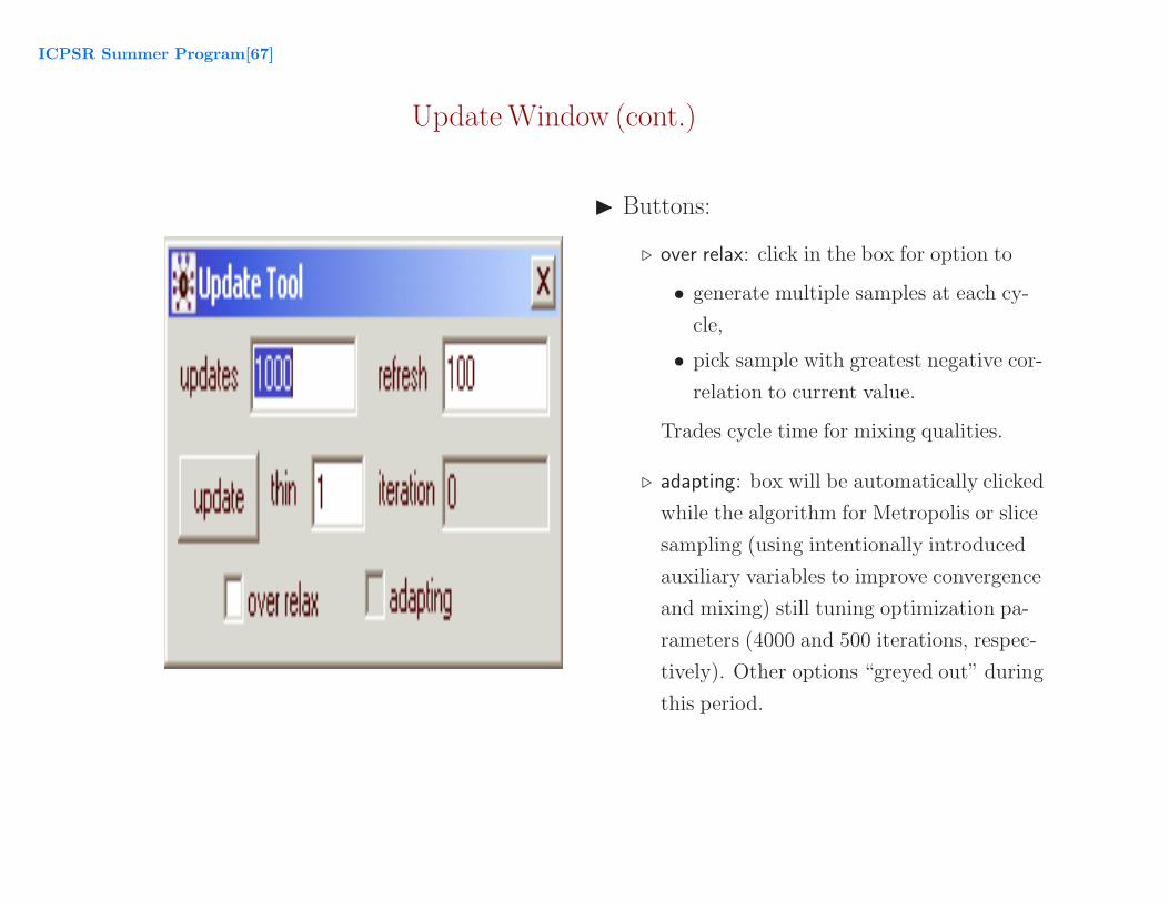
Update Window (cont.)

� Buttons:

� over relax: click in the box for option to

• generate multiple samples at each cy-

cle,

• pick sample with greatest negative cor-

relation to current value.

Trades cycle time for mixing qualities.

� adapting: box will be automatically clicked

while the algorithm for Metropolis or slice

sampling (using intentionally introduced

auxiliary variables to improve convergence

and mixing) still tuning optimization pa-

rameters (4000 and 500 iterations, respec-

tively). Other options “greyed out” during

this period.


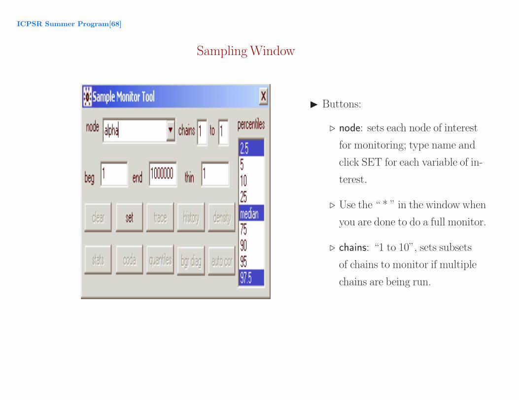
Sampling Window

� Buttons:

� node: sets each node of interest

for monitoring; type name and

click SET for each variable of in-

terest.

� Use the “ * ” in the window when

you are done to do a full monitor.

� chains: “1 to 10”, sets subsets

of chains to monitor if multiple

chains are being run.


Sampling Window

� Buttons, cont.:

� beg, end: the beginning and end-

ing chain values current to be

monitored. BEG is 1 unless you

know the burn-in period.

� thin: yet another opportunity to

thin the chain.

� clear: clear a node from being

monitored.


Sampling Window

� Buttons, cont.:

� trace: do dynamic traceplots for

monitored nodes.

� history: display a traceplot for

the complete history.

� density: display a kernel density

estimate.


Sampling Window

� Buttons, cont.:

� quantiles: displays running mean

with running 95% CI by iteration

number.

� auto cor: plots of autocorrela-

tions for each node with lags 1 to

50.

� coda: display chain history in

window in CODA format, an-

other window appears with

CODA ordering information.


Sampling Window

� Buttons, cont.:

� stats: summary statistics on

each monitored node using:

mean, sd, MC error, current it-

eration value, starting point of

chain and percentiles from PER-

CENTILES window.

� Notes on stats:

WinBUGS regularly pro-

vides both: naive SE =

sample variance/√

n

and: MC Error =√spectral density var/

√n =

asymptotic SE.

ICPSR/Bayes: Modeling and Analysis using MCMC Methods [46]

Basic Structure of the BHM

I Start with the most basic model setup for producing a posterior:

π(θ|D) ∝ L(θ|D)p(θ).

I Now suppose that θ is conditional on another quantity ψ, so that the calculation of the posterior

becomes:

π(θ, ψ|D) ∝ L(θ|D)p(θ|ψ)p(ψ).

I θ still has a prior distribution, p(θ|ψ), but it is now conditional on another parameter that has its

own prior, p(ψ), called a hyperprior, which now has its own hyperparameters.

I Inference for either parameter of interest can be obtained from the marginal densities:

π(θ|D) =

∫

ψ

π(θ, ψ|D)dψ

π(ψ|D) =

∫

θ

π(θ, ψ|D)dθ.


Basic Structure of the BHM (cont.)

I We can continue stringing hyperpriors to the right:

π(θ, ψ, ζ|D) ∝ L(θ|D)p(θ|ψ)p(ψ|ζ)p(ζ).

I Now ζ is the highest level parameter and therefore the only hyperprior that is unconditional.

I Marginal for the new conditional obtained the same way:

π(ψ|D) =

∫

ζ

π(ψ, ζ|D)dζ.

I No real restriction to the number of levels but increasing levels have decreasing conditional

amount of sample information, and lower model utility. See Goel and Degroot (1981) or Goel

(1983) for a formalization of the conditional amount of sample information (CASI).


A Poisson-Gamma Hierarchical Model

I Consider the following model with priors and hyperpriors:

yi

λi

Gλ(αi, βi)

Gα(A,B) Gβ(C,D)

Observed Values

Poisson Parameter

Gamma Prior

Gamma Hyperpriors


A Poisson-Gamma Hierarchical Model (cont.)

I Notes on this model:

. The intensity parameter of the Poisson distribution is now indexed by i since it is no longer as-

sumed to be a fixed effect.

. Now: λi ∼ G(α, β).

. Model expressed in “stacked” notation:

yi ∼ P(λi)

λi ∼ G(α, β)

α ∼ G(A,B)

β ∼ G(C,D),

where the yi are assumed conditionally independent and α and β are assumed independent.



I The joint posterior distribution of interest is:

p(λ,y, α, β) =

n∏

i=1

p(yi|λi)p(λi|α, β)p(α|A,B)p(β|C,D)

=n∏

i=1

[

(yi!)−1λyii exp(−λi)βαΓ(α)−1exp(−λiβ)λα−1

i

×BAΓ(A)−1exp(−αB)αA−1DCΓ(C)−1exp(−βD)βC−1

]

,

so:

p(λi,y, α, β) ∝ λ∑yi+α−1

i αA−1βα+C−1Γ(α)−1 exp[−λi(1 + β) − αB − βD].

which is unpleasant.



! Recall that if we can get the full conditional distributions for each of the coe!cients in the poste-

rior, we can run the Gibbs sampler and obtain the marginal posterior distributions with MCMC.

!("|#, $) =p(", #, $|y)

p(#, $|y)=

p(", #, $)

p(#, $)=

p(", #, $)

p(#)p($)

! "!

yi+#"1exp[""(1 + $)]

# G("

yi + #, 1 + $).

! So given (interim) values for # and $, we can sample from the distribution for ".

! The easy part: p(#|$, ") = p(#), and p($|#, ") = p($), by the initial assumptions of the hierarchi-

cal model.

∼ G��

yi + α, n+ β�.

∝ λ�

yi+α−1 exp [−λ (β + n)]

Documents

Applied Bayesian Analysis for the Social Sciences Day 3 ...spia.uga.edu/faculty_pages/rbakker/bayes/Day3_winbugs.pdfFlorida State University Bayesian Workshop Applied Bayesian Analysis