Applications of Sorting

The key to understanding sorting is seeing how it can be usedto solve many important programming tasks:

• Uniqueness Testing– How can we test if the elements ofa given collection of itemsS are all distinct?

• Deleting Duplicates– How can we remove all but onecopy of any repeated elements inS?

• Median/Selection– How can we find thekth largest itemin setS?

• Frequency Counting – Which is the most frequentlyoccurring element inS, i.e., the mode?

• Reconstructing the Original Order– How can we restorethe original arrangement of a set of items after we permutethem for some application?

• Set Intersection/Union– How can we intersect or unionthe elements of two containers?

• Finding a Target Pair – How can we test whether thereare two integersx, y ∈ S such thatx + y = z for sometargetz?

• Efficient Searching– How can we efficiently test whetherelements is in setS?

Basic Sorting Algorithms

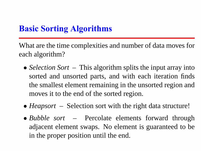
What are the time complexities and number of data moves foreach algorithm?

• Selection Sort– This algorithm splits the input array intosorted and unsorted parts, and with each iteration findsthe smallest element remaining in the unsorted region andmoves it to the end of the sorted region.

• Heapsort – Selection sort with the right data structure!

• Bubble sort – Percolate elements forward throughadjacent element swaps. No element is guaranteed to bein the proper position until the end.

• Insertion Sort– This algorithm also maintains sorted andunsorted regions of the array. In each iteration, the nextunsorted element moves up to its appropriate position inthe sorted region.

• Quicksort – This algorithm reduces the job of sortingone big array into the job of sorting two smaller arraysby performing apartition step. The partition separatesthe array into those elements that are less than thepivot/divider element, and those which are strictly greaterthan this pivot/divider element.

Multicriteria Sorting

How can we break ties in sorting using multiple criteria, likesorting first on last name breaking ties on first name?One way is to use a complicated comparison function thatcombines all the keys to break ties:int suitor_compare(suitor *a, suitor *b){

int result; /* result of comparison */

if (a->height < b->height) return(-1);if (a->height > b->height) return(1);

if (a->weight < b->weight) return(-1);if (a->weight > b->weight) return(1);

if ((result=strcmp(a->last,b->last)) != 0)return result;

return(strcmp(a->first,b->first));}

Stable Sorting

Another way is to use repeated passes through astablesortingfunction, one which is guaranteed to leave identical keys inthe same relative order they were in before the sorting.If so, we could sort by first name, and then do stable sort bylast name and know the final results are sorted by both majorand minor keys.STL provides a stable sorting routine, where keys of equalvalue are guaranteed to remain in the same relative order.void stable_sort(RandomAccessIterator bg, RandomAccessIterator end)void stable_sort(RandomAccessIterator bg, RandomAccessIterator end,

BinaryPredicate op)

Sorting Library Functions in C

The stdlib.h contains library functions for sorting andsearching. For sorting, there is the functionqsort:#include <stdlib.h>

void qsort(void *base, size_t nel, size_t width,int (*compare) (const void *, const void *));

It sorts the firstnel elements of an array (pointed to bybase), where each element iswidth-bytes long. Thus wecan sort arrays of 1-byte characters, 4-byte integers, or 100-byte records, all by changing the value ofwidth.Binary search is also included:

bsearch(key, (char *) a, cnt, sizeof(int), intcompare);

Comparison Functions

The ultimate desired order is determined by the functioncompare. It takes as arguments pointers to twowidth-byteelements, and returns a negative number if the first belongsbefore the second in sorted order, a positive number if thesecond belongs before the first, or zero if they are the same.

Sorting and Searching in C++

The C++ Standard Template Library (STL) includes methodsfor sorting, searching, and more. Serious C++ users shouldget familiar with STL.To sort with STL, we can either use the default comparison(e.g.,≤) function defined for the class, or override it with aspecial-purpose comparison functionop:void sort(RandomAccessIterator bg, RandomAccessIterator end)void sort(RandomAccessIterator bg, RandomAccessIterator end,

BinaryPredicate op)

STL Sorting Applications

Other STL functions implement some of the applications ofsorting, including,

• nth element – Return the nth largest item in thecontainer.

• set union, set intersection,set difference – Construct the union, intersection,and set difference of two containers.

predicate

• unique – Remove all consecutive duplicates.

Sorting and Searching in Java

Thejava.util.Arrays class contains various methodsfor sorting and searching. In particular,static void sort(Object[] a)static void sort(Object[] a, Comparator c)

sorts the specified array of objects into ascending orderusing either the natural ordering of its elements or a specificcomparatorc. Stable sorts are also available.Methods for searching a sorted array for a specified objectusing either the natural comparison function or a newcomparatorc are also provided:binarySearch(Object[] a, Object key)binarySearch(Object[] a, Object key, Comparator c)

110401 (Vito’s Family)

Find the most central location on a street, to minimize totaldistance to certain neighbors.Is the right version of average mean, median, or somethingelse?

110403 (Bridge)

How shouldn people of variable speeds cross a two-manbridge at night when there is only one flashlight?Does sorting the people by speed help determine who shouldbe paired up?

110405 (Shoemaker’s Problem)

How should a shoemaker order the jobs he does so as tominimize total penalty costs for lateness, when different jobshave different penalties?Does it help to sort jobs by their length, or by their penalty,or both?

110406 (CDVII)

Compute the total amount of tolls people owe in a worldwhere toll costs vary with time.How do we pair up entry and exit records?

How Long is Long?

Today’s PCs are typically 32-bit machines, so standardinteger data types supports integers roughly in the range±2

31= ± 2,147,483,648. Thus we can safely count up to a

billion or so with standard integers on conventional machines.We can get an extra bit by usingunsigned integers.Most programming languages supportlong or evenlonglong integer types, which define 64-bit or occasionally 128-bit integers. 2

63= 9,223,372,036,854,775,808, so we are

talking very large numbers!

Floating Point Precision

The magnitude of numbers which can be represented asfloat s is astonishingly large, particularly with double-precision. This magnitude comes by representing the numberin scientific notation, asa × 2

c. Sincea and c are bothrestricted to a given number of bits, there is still only a limitedprecision.Thus don’t be fooled into thinking thatfloat s give you theability to count to very high numbers. Use integers and longsfor such purposes.

Representing Enormous-Precision Integers

Representing truly enormous integers requires stringingdigits together. Two possible representations are —

• Arrays of Digits – The easiest representation forlong integers is as an array of digits, where the initialelement of the array represents the least significant digit.Maintaining a counter with the length of the number indigits can aid efficiency by minimizing operations whichdon’t affect the outcome.

• Linked Lists of Digits – Dynamic structures are necessaryif we arereally going to do arbitrary precision arithmetic,i.e., if there is no upper bound on the length of thenumbers. Note, however, that 100,000-digit integers arepretty long yet can be represented using arrays of only100,000 bytes each.

What dynamic memoryreally provides is the freedom to usespace where you need it. If you wanted to create a large arrayof high-precision integers, most of which were small,thenyou would be better off with a list-of-digits representation.

Bignum Data Type

Our bignum data type is represented as follows:#define MAXDIGITS 100 / * maximum length bignum * /

#define PLUS 1 / * positive sign bit * /#define MINUS -1 / * negative sign bit * /

typedef struct {char digits[MAXDIGITS]; / * represent the number * /int signbit; / * PLUS or MINUS * /int lastdigit; / * index of high-order digit * /

} bignum;

AdditionAdding two integers is done from right to left, with anyoverflow rippling to the next field as a carry. Allowingnegative numbers turns addition into subtraction.add_bignum(bignum * a, bignum * b, bignum * c){

int carry; / * carry digit * /int i; / * counter * /

initialize_bignum(c);

if (a->signbit == b->signbit) c->signbit = a->signbit;else {

if (a->signbit == MINUS) {a->signbit = PLUS;subtract_bignum(b,a,c);a->signbit = MINUS;

} else {b->signbit = PLUS;subtract_bignum(a,b,c);b->signbit = MINUS;

}return;

}

c->lastdigit = max(a->lastdigit,b->lastdigit)+1;carry = 0;

for (i=0; i<=(c->lastdigit); i++) {c->digits[i] = (char)

(carry+a->digits[i]+b->digits[i]) % 10;carry = (carry + a->digits[i] + b->digits[i]) / 10;

}

zero_justify(c);}

Signbits

Manipulating the signbit is a non-trivial headache. Wereduced certain cases to subtraction by negating the numbersand/or permuting the order of the operators, but took care toreplace the signs first.The actual addition is quite simple, and made simpler byinitializing all the high-order digits to 0 and treating the finalcarry over as a special case of digit addition.

Zero Justif cation

The zero justify operation adjustslastdigit toavoid leading zeros. It is harmless to call after everyoperation, particularly as it corrects for−0:zero_justify(bignum * n){

while ((n->lastdigit > 0) && (n->digits[ n->lastdigit ]==0))n->lastdigit --;

if ((n->lastdigit == 0) && (n->digits[0] == 0))n->signbit = PLUS; / * hack to avoid -0 * /

}

Subtraction

Subtraction is trickier than addition because it requiresborrowing. To ensure that borrowing terminates, it is bestto make sure that the larger-magnitude number is on top.subtract_bignum(bignum * a, bignum * b, bignum * c) {

int borrow; / * anything borrowed? * /int v; / * placeholder digit * /int i; / * counter * /

if ((a->signbit == MINUS) || (b->signbit == MINUS)) {b->signbit = -1 * b->signbit;add_bignum(a,b,c);b->signbit = -1 * b->signbit;return;

}if (compare_bignum(a,b) == PLUS) {

subtract_bignum(b,a,c);c->signbit = MINUS;return;

}c->lastdigit = max(a->lastdigit,b->lastdigit);borrow = 0;for (i=0; i<=(c->lastdigit); i++) {

v = (a->digits[i] - borrow - b->digits[i]);if (a->digits[i] > 0)

borrow = 0;if (v < 0) {

v = v + 10;borrow = 1;

}c->digits[i] = (char) v % 10;

}zero_justify(c);

}

ComparisonDeciding which of two numbers is larger requires a compari-son operation. Comparison proceeds from highest-order digitto the right, starting with the sign bit:compare_bignum(bignum * a, bignum * b){

int i; / * counter * /

if ((a->signbit==MINUS) && (b->signbit==PLUS)) return(PLUS);if ((a->signbit==PLUS) && (b->signbit==MINUS)) return(MINUS);if (b->lastdigit > a->lastdigit) return (PLUS * a->signbit);if (a->lastdigit > b->lastdigit) return (MINUS * a->signbit);

for (i = a->lastdigit; i>=0; i--) {if (a->digits[i] > b->digits[i])

return(MINUS * a->signbit);if (b->digits[i] > a->digits[i])

return(PLUS * a->signbit);}return(0);

}

Multiplication

Multiplication seems like a more advanced operation thanaddition or subtraction. A people as sophisticated as theRomans had a difficult time multiplying, even though theirnumbers look impressive on building cornerstones and SuperBowls.The Roman’s problem was that they did not use a radix (orbase) number system. Certainly multiplication can be viewedas repeated addition and thus solved in that manner, but it willbe hopelessly slow. Squaring 999,999 by repeated additionrequires on the order of a million operations, but is easilydoable by hand using the row-by-row method we learned inschool.

Schoolhouse Multiplication

multiply_bignum(bignum * a, bignum * b, bignum * c){

bignum row; / * represent shifted row * /bignum tmp; / * placeholder bignum * /int i,j; / * counters * /

initialize_bignum(c);

row = * a;

for (i=0; i<=b->lastdigit; i++) {for (j=1; j<=b->digits[i]; j++) {

add_bignum(c,&row,&tmp);

* c = tmp;}digit_shift(&row,1);

}

c->signbit = a->signbit * b->signbit;zero_justify(c);

}

Each operation involves shifting the first number one moreplace to the right and then adding the shifted first numberd times to the total, whered is the appropriate digit of thesecond number.We might have gotten fancier than using repeated addition,but since the loop cannot spin more than nine times per digit,any possible time savings will be relatively small.

Digit Shift

Shifting a radix-number one place to the right is equivalentto multiplying it by the base of the radix, or 10 for decimalnumbers:digit_shift(bignum * n, int d) / * multiply n by 10ˆd * /{

int i; / * counter * /

if ((n->lastdigit == 0) && (n->digits[0] == 0)) return;

for (i=n->lastdigit; i>=0; i--)n->digits[i+d] = n->digits[i];

for (i=0; i<d; i++) n->digits[i] = 0;

n->lastdigit = n->lastdigit + d;}

Exponentiation

Exponentiation is repeated multiplication, and hence subjectto the same performance problems as repeated addition onlarge numbers. The trick is to observe that

an= an÷2

× an÷2× anmod2

so it can be done using only a logarithmic number ofmultiplications.

Division

Although long division is an operation feared by schoolchil-dren and computer architects, it too can be handled with asimpler core loop than might be imagined.Division by repeated subtraction is again far too slow to workwith large numbers, but the basic repeated loop of shifting theremainder to the left, including the next digit, and subtractingoff instances of the divisor is far easier to program than“guessing” each quotient digit as we were taught in school:

Division Code

divide_bignum(bignum * a, bignum * b, bignum * c){

bignum row; / * represent shifted row * /bignum tmp; / * placeholder bignum * /int asign, bsign; / * temporary signs * /int i,j; / * counters * /

initialize_bignum(c);

c->signbit = a->signbit * b->signbit;

asign = a->signbit;bsign = b->signbit;

a->signbit = PLUS;b->signbit = PLUS;

initialize_bignum(&row);initialize_bignum(&tmp);

c->lastdigit = a->lastdigit;

for (i=a->lastdigit; i>=0; i--) {di git_shift(&row,1);row.digits[0] = a->digits[i];c->digits[i] = 0;while (compare_bignum(&row,b) != PLUS) {

c->digits[i] ++;subtract_bignum(&row,b,&tmp);row = tmp;

}}

zero_justify(c);

a->signbit = asign;b->signbit = bsign;

}

Computing the Remainder

This routine performs integer division and throws away theremainder. If you want to compute the remainder ofa ÷ b,you can always doa − b(a ÷ b).

Numerical Bases and ConversionThe digit representation of a given radix-number is a functionof which numericalbase is used. Particularly interestingnumerical bases include:

• Binary – Base-2 numbers are made up of the digits 0 and1. They provide the integer representation used withincomputers, because these digits map naturally to on/off orhigh/low states.

• Octal – Base-8 numbers are useful as a shorthand tomake it easier to read binary numbers, since the bitscan be read off from the right in groups of three. Thus101110012 = 3718 = 24910. Why do programmers thinkChristmas is Halloween? Because 31 Oct = 25 Dec!

• Decimal – We use base-10 numbers because we learnedto count on our ten fingers.

• Hexadecimal – Base-16 numbers are an even easiershorthand to represent binary numbers, once you get overthe fact that the digits representing 10 through 15 are “A”to ‘’F.”

• Alphanumeric – Occasionally, one sees even highernumerical bases. Base-36 numbers are the highest youcan represent using the 10 numerical digits with the 26letters of the alphabet. Any integer can be represented inbase-X provided you can displayX different symbols.

Base Conversion

There are two distinct algorithms you can use to convert base-a numberx to a base-b numbery —

• Left to Right – Here, we find the most-significant digit ofy first. It is the integerdl such that

(dl + 1)bk > x ≥ dlbk

where1 ≤ dl ≤ b − 1. In principle, this can be found bytrial and error, although you must to be able to comparethe magnitude of numbers in different bases. This isanalogous to the long-division algorithm described above.

• Right to Left – Here, we find the least-significant digitof y first. This is the remainder ofx divided by b.Remainders are exactly what is computed when doingmodular arithmetic. The cute thing is that we can computethe remainder ofx on a digit-by-digit basis, making it easyto work with large integers.

Right-to-left translation is similar to how we translatedconventional integers to our bignum presentation. Taking thelong integer mod 10 (using the%operator) enables us to peeloff the low-order digit.

110502 (Reverse and Add)

Does repeatedly adding a number to its digit-reversaleventually end on a palindrome?

110503 (The Archeologists’ Dilemma)

What is the smallest power of 2 begining with the given digitsequence?

110504 (Ones)

How many digits is the smallest multiple ofn such that theresulting digit sequence is all 1s? Why is this possible forevery non-multiple of 2 and 5?

110505 (A multiplication game)

What is the right strategy for a two-person digit multiplicationgame?Is it recursive/minimax?

Learning to CountCombinatorics problems are notorious for their reliance oncleverness and insight. Once you look at the problem in theright way, the answer suddenly becomes obvious.Basic counting techniques include:

• Product Rule – Theproduct rulestates that if there are|A| possibilities from setA and|B| possibilities from setB, then there are|A| × |B| ways to combine one fromAand one fromB.

• Sum Rule – The sum rulestates that if there are|A|

possibilities from setA and|B| possibilities from setB,then there are|A|+ |B| ways for eitherA or B to occur –assuming the elements ofA andB are distinct.

Inclusion-Exclusion Formula

The sum rule is a special case of a more general formula whenthe two sets can overlap, namely,

|A ∪ B| = |A| + |B| − |A ∩ B|

The reason this works is that summing the sets double countscertain possibilities, namely, those occurring in both sets.Double counting is a slippery aspect of combinatorics,which can make it difficult to solve problems via inclusion-exclusion.

Combinatorial Objects

A bijection is a one-to-one mapping between the elements ofone set and the elements of another. Counting the size of oneof the sets automatically gives you the size of the other set.Exploiting bijections requires us to have a repertoire of setswhich we know how to count, so we can map other objects tothem.It is useful to have a feeling for how fast the number of objectsgrows, to know when exhaustive search breaks down as apossible technique:

Permutations

A permutationis an arrangement ofn items, where every itemappears exactly once.There aren! =

∏ni=1

i different permutations. The3! = 6

permutations of three items are 123, 132, 213, 231, 312, and321.Forn = 10, n! = 3, 628, 800.

Subsets

A subsetis a selection of elements fromn possible items.There are2n distinct subsets ofn things.Thus there are23

= 8 subsets of three items, namely, 1, 2, 3,12, 13, 23, 123, and the empty set: never forget the empty set.Forn = 20, 2

n= 1, 048, 576.

Strings

A string is a sequence of items which are drawnwithrepetition.There aremn distinct sequences ofn items drawn fromm

items. There are 27 length-3 strings on 123.The number of binary strings of lengthn is identical to thenumber of subsets ofn items (why?)

Recurrence Relations

Recurrence relations make it easy to count a variety ofrecursively defined structures. Recursively defined structuresinclude trees, lists, well-formed formulae, and divide-and-conquer algorithms – so they lurk wherever computerscientists do.A recurrence relation is an equation which is defined in termsof itself, such as the Fibonacci numbers:

Fn = Fn−1 + Fn−2

Why Recurrence Relations?

They are useful because many natural functions are easilyexpressed as recurrences:Polynomials:

an = an−1 + 1, a1 = 1 −→ an = n

Exponentials:

an = 2an−1, a1 = 2 −→ an = 2n

Weird but interesting functions otherwise hard to represent:

an = nan−1, a1 = 1 −→ an = n!

It is often easy to find a recurrence as the answer to a countingproblem.

Closed Form Solutions of Recurrences

Solving the recurrence to get a nice closed form can besomewhat of an art, but as we shall see, computer programscan easily evaluate the value of a given recurrence evenwithout the existence of a nice closed form.

Binomial Coeff cientsThe most important class of counting numbers are thebinomial coefficients, where(n

k) counts the number of waysto choosek things out ofn possibilities. What do they count?

• Committees– How many ways are there to form ak-member committee fromn people? By definition,(n

k) isthe answer.

• Paths Across a Grid– How many ways are there to travelfrom the upper-left corner of ann × m grid to the lower-right corner by walking only down and to the right? Everypath must consist ofn + m steps,n downward andm tothe right. Every path with a different set of downwardmoves is distinct, so there are(n + m

n ) such sets/paths.

• Coefficients of(a + b)n – Observe that

(a + b)3 = 1a3+ 3a2b + 3ab2

+ 1b3

What is the coefficient of the termakbn−k? Clearly(n

k),because it counts the number of ways we can choose thek a-terms out ofn possibilities.

Computing Binomial Coeff cients

Since(n

k) = n!/((n − k)!k!), in principle you can computethem straight from factorials. However, intermediatecalculations can easily cause arithmetic overflow even whenthe final coefficient fits comfortably within an integer.A more stable way to compute binomial coefficients is usingthe recurrence relation implicit in the construction of Pascal’striangle, namely, that

(n

k) = (n − 1

k − 1) + (n − 1

k )

Why Pascal?

Consider whether thenth element appears in one of the(n

k)

subsets ofk elements. If so, we can complete the subset bypickingk−1 other items from the othern−1. If not, we mustpick all k items from the remainingn−1. There is no overlapbetween these cases, and all possibilities are included, so thesum counts allk-subsets.No recurrence is complete without basis cases. How manyways are there to choose 0 things from a set? Exactly one, theempty set. The right term of the sum drives us up to(

k

k). Howmany ways are there to choosek things from ak-element set?Exactly one, the complete set.

Implementation

The following implementation of this recurrence is a goodexample of programming techniques used indynamic pro-gramming, namely storing a table of results so we canevaluate terms of the recurrence by looking up the appropriatevalues.#define MAXN 100 /* largest n or m */

long binomial_coefficient(n,m)int n,m; /* computer n choose m */{

int i,j; /* counters */long bc[MAXN][MAXN]; /* table of binomial coefficients */

for (i=0; i<=n; i++) bc[i][0] = 1;

for (j=0; j<=n; j++) bc[j][j] = 1;

for (i=1; i<=n; i++)for (j=1; j<i; j++)

bc[i][j] = bc[i-1][j-1] + bc[i-1][j];

return( bc[n][m] );}

Other Counting Sequences

Several other counting sequences which repeatedly emerge inapplications, and which are easily computed using recurrencerelations.

• Fibonacci numbers – Defined by the recurrenceFn = Fn−1 + Fn−2 and the initial valuesF0 = 0 andF1 = 1, they emerge repeatedly because this is perhaps thesimplest interesting recurrence relation. The first severalvalues are 0, 1, 1, 2, 3, 5, 8, 13, 21, 34, 55, . . .

Catalan Numbers

The recurrence and associated closed form

Cn =n−1∑

k=0

CkCn−1−k =1

n + 1(

2n

n)

defines theCatalan numbers, which occur in a surprisingnumber of problems in combinatorics. The first several termsare2, 5, 14, 42, 132, 429, 1430, . . . whenC0 = 1.How many ways are there to build a balanced formula fromn

sets of left and right parentheses? For example, there are fiveways to do it forn = 3: ((())), ()(()), (())(), (()()), and()()().The leftmost parenthesisl matches some right parenthesisr,which must partition the formula into two balanced pieces,leading to the recurrence.

The exact same reasoning arises in counting the number oftriangulations of a convex polygon, counting the number ofrooted binary trees onn + 1 leaves, and counting the numberof paths across a lattice which do not rise above the maindiagonal.

Eulerian Numbers

TheEuleriannumbers〈n

k〉 count the number of permutationsof lengthn with exactlyk ascending sequences orruns. A re-currence can be formulated by considering each permutationp of 1, ..., n − 1. There aren places to insert elementn, andeach either splits an existing run ofp or occurs immediatelyafter the last element of an existing run, thus preserving therun count. Thus〈n

k〉 = k〈n − 1

k 〉 + (n − k + 1)〈n − 1

k − 1〉.

Integer Partitions

An integer partition ofn is an unordered set of positiveintegers which add up ton. For example, there are sevenpartitions of 5, namely,(5), (4, 1), (3, 2), (3, 1, 1), (2, 2, 1),(2, 1, 1, 1), and(1, 1, 1, 1, 1). The easiest way to count themis to define a functionf(n, k) giving the number of integerpartitions ofn with largest part at mostk. In any acceptablepartition the largest part either does or does not reach withlimit, so f(n, k) = f(n− k, k) + f(n, k− 1). The basis casesaref(1, 1) = 1 andf(n, k) = 0 wheneverk > n.

110603 (Counting)

How many ways can we expressn asthe sum of 2s, 3s, andtwo types of 1?

110604 (Expressions)

How many ways can we build a well-formed formula fromnparentheses with nesting depthd?

110606 (The Priest Mathematician)

What is the best way to solve a 4-peg Tower of Hanoi puzzle?

110607 (Self-describing Sequence)

What is the ith value of the sequence containingf(k)

occurrences ofk for eachk, i.e. 1, 2, 2, 3, 3, 4 ,4, 4, 5, 5,5, 6 . . . ?What if i is too large to construct the entire sequence inmemory?

Number Theory and Divisibility

“G-d created the integers. All else is the work of man.”– Kronecker.

Number theory is the study of the properties of the integers,specifically integer divisibility. It is a fascinating area isbeautiful proofs and surprising results.We sayb divides a (denotedb|a) if a = bk for some integerk.Equivalently, we say thatb is adivisor of a or a is amultipleof b if b|a.As a consequence of this definition, the smallest naturaldivisor of every non-zero integer is 1. In general there is nointegerk such thata = 0 · k.

Prime Numbers

A prime number is an integerp > 1 which is only divisibleby 1 and itself.Said another way, ifp is a prime number, thenp = a · b forintegersa ≤ b implies thata = 1 andb = p.The fundamental theorem of arithmetic. states is that everyinteger can be expressed in only one way as the product ofprimes. 105 is uniquely expressed as3 × 5 × 7, and32 isuniquely expressed as2 × 2 × 2 × 2 × 2.This unique set of numbers multiplying ton is called theprime factorization of n.Any number which is not prime is said to becomposite.

Primality Testing and Factorization

Not only are there an infinite number of primes (see Euclid’sproof), but there are a lot of them. There are roughlyx/ ln x

primes less than or equal tox, i.e. roughly one out of everyln x numbers is prime.The easiest way to find the prime factorization of an integern is repeated division. Note the that smallest prime factor ismust at most

√n unlessn is prime.

Constructing all Divisors

Every divisor is the product of some subset of these primefactors. Such subsets can be constructed using backtrackingtechniques, but we must be careful about duplicate primefactors.For example, the prime factorization of 12 has three terms (2,2, and 3) but 12 has only 6 divisors (1, 2, 3, 4, 6, 12).

Greatest Common Divisor

The greatest common divisor, or gcd, the largest divisorshared by a given pair of integers. The reduced form of thefraction24/36 comes after we divide both the numerator anddenominator bygcd(x, y), in this case 12.Euclid’s GCD algorithm rests on two observations. First,

If b|a, thengcd(a, b) = b.

This should be pretty clear. Ifb dividesa, thena = bk forsome integerk, and thusgcd(bk, b) = b. Second,

If a = bt + r for integerst and r, thengcd(a, b) =

gcd(b, r).

Why? By definition,gcd(a, b) = gcd(bt+ r, b). Any commondivisor of a andb must rest totally withr, becausebt clearlymust be divisible by any divisor ofb.It can also find integersx andy such that

a · x + b · y = gcd(a, b)

which will prove quite useful in solving linear congruences.

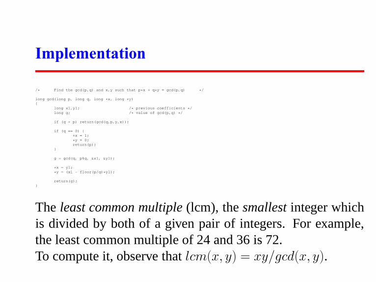
Implementation

/* Find the gcd(p,q) and x,y such that p*x + q*y = gcd(p,q) */

long gcd(long p, long q, long *x, long *y){

long x1,y1; /* previous coefficients */long g; /* value of gcd(p,q) */

if (q > p) return(gcd(q,p,y,x));

if (q == 0) {

*x = 1;

*y = 0;return(p);

}

g = gcd(q, p%q, &x1, &y1);

*x = y1;

*y = (x1 - floor(p/q)*y1);

return(g);}

The least common multiple (lcm), thesmallest integer whichis divided by both of a given pair of integers. For example,the least common multiple of 24 and 36 is 72.To compute it, observe thatlcm(x, y) = xy/gcd(x, y).

Modular Arithmetic

Sometimes computing the remainder is more important thana quotient.What day of the week will your birthday fall on next year?All you need to know is the remainder of the number of daysbetween now and then (either 365 or 366) when dividing bythe 7 days of the week. Thus it will fall on this year’s dayplus one (365mod7) or two (366mod7) days, depending uponwhether it is affected by a leap year.The key to such efficient computations ismodular arithmetic.The number we are dividing by is called themodulus, and theremainder left over is called theresidue.

What is(x + y)modn? We can simplify this to

((xmodn) + (ymodn))modn

to avoid adding big numbers.Subtraction s just a special case of addition.

(12mod100)− (53mod100) =−41mod100 = 59mod100

Notice how we can convert a negative number modn to apositive number by adding a multiple ofn to it.

Exponentiation

Since multiplication is just repeated addition,

xymod n = (xmodn)(ymodn)modn

Since exponentiation is just repeated multiplication,

xymodn= (xmodn)ymodn

Since exponentiation is the quickest way to produce reallylarge integers, this is where modular arithmetic really provesits worth.Division proves considerably more complicated to dealwith. . .

What is the Last Digit?

What is the last digit of2100? We can do this computation byhand. What we really want to know is what2

100mod10 is. Bydoing repeated squaring, and taking the remainder mod10 ateach step we make progress very quickly:

23mod10 = 8

26mod10 = 8× 8mod10→ 4

212mod10 = 4× 4mod10→ 6

224mod10 = 6× 6mod10→ 6

248mod10 = 6× 6mod10→ 6

296mod10 = 6× 6mod10→ 6

2100mod10 = 2

96× 2

3× 2

1mod10→ 6

Congruences

Congruences are an alternate notation for representingmodular arithmetic. We say thata ≡ b(modm) if m|(a − b).By definition, if amodm is b, thena ≡ b(modm).It gets us thinking about theset of integers with a givenremaindern, and gives us equations for representing them.What integersx satisfy the congruencex ≡ 3(mod9)? Theset of solutions is all integers of the form9y + 3, wherey isany integer.What about2x ≡ 3(mod9) and2x ≡ 3(mod4)?Trial and error should convince you that exactly the integersof the form9y + 6 satisfy the first example, while the secondhas no solutions at all.

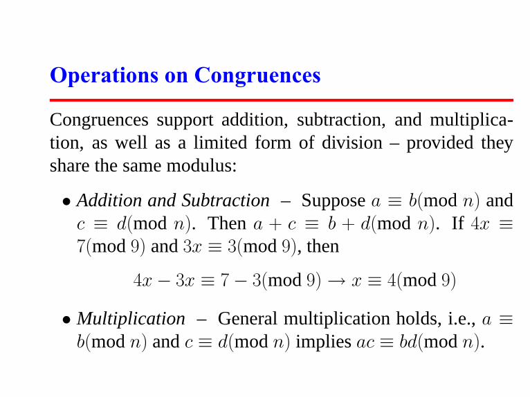
Operations on Congruences

Congruences support addition, subtraction, and multiplica-tion, as well as a limited form of division – provided theyshare the same modulus:

• Addition and Subtraction – Supposea ≡ b(modn) andc ≡ d(mod n). Thena + c ≡ b + d(mod n). If 4x ≡

7(mod9) and3x ≡ 3(mod9), then

4x − 3x ≡ 7 − 3(mod9) → x ≡ 4(mod9)

• Multiplication – General multiplication holds, i.e.,a ≡

b(modn) andc ≡ d(modn) impliesac ≡ bd(modn).

• Division – We cannot cavalierly cancel common factorsfrom congruences. Note that6 · 2 ≡ 6 · 1(mod 3), butclearly2 6≡ 1(mod3).

Note that division can be defined as multiplication by aninverse, soa/b is equivalent toab−1. But this inverse doesnot always exist – try to find a solution to2x ≡ 1(mod4).

Simplifying and Solving Congruences

We can simplify a congruencead ≡ bd(mod dn) toa ≡ b(modn), so we can divide all three terms by a mutuallycommon factor if one exists. Thus170 ≡ 30(mod 140)

implies that17 ≡ 3(mod14).A linear congruence is an equation of the formax ≡

b(mod n). Solving this equation means identifying whichvalues ofx satisfy it.Not all such equations have solutions.ax ≡ 1(mod n)

has a solution if and only if the modulus and the multiplierare relatively prime, i.e.,gcd(a, n) = 1. We may useEuclid’s algorithm to find this inverse through the solutionto a · x′

+ n · y′ = gcd(a, n) = 1.

In general, there are three cases, depending on the relation-ship betweena, b, andn:

• gcd(a, b, n) > 1 – Then we can divide all three terms bythis divisor to get an equivalent congruence. This givesus a single solution mod the new base, or equivalentlygcd(a, b, n) solutions(modn).

• gcd(a, n) does not divide b – The congruence can haveno solution.

• gcd(a, n) = 1 – Then there is one solution(mod n).Further,x = a−1b works, sinceaa−1b ≡ b(modn). Thisinverse exists and can be found using Euclid’s algorithm.

More Advanced Tools

The Chinese remainder theorem gives us a tool for workingwith systems of congruences over different moduli. Supposethere is exists an integerx such thatx ≡ a1(modm1) andx ≡

a2(modm2). Thenx is uniquely determined(modm1m2) ifm1 andm2 are relatively prime.

Diophantine Equations

Diophantine equations are formulae in which the variablesare restricted to integers. For example, Fermat’s last theoremconcerned answers to the equationan

+ bn= cn.

The most important class are linear Diophantine equations ofthe formax−ny = b, wherex andy are the integer variablesanda, b, andn are integer constants. These are readily shownto be equivalent to the solving the congruenceax ≡ b(modn)

and hence can be solved using the techniques above.

110702 (Carmichael Numbers)

Which composite integersn always satisfy the equation

anmodn= a

Does this require large integer arithmetic?

110704 (Factovisors)

Doesa dividen!?Does this require large integer arithmetic?

110707 (Marbles)

What is the cheapest way to perfectly storen among twotypes of boxes?

110708 (Repackaging)

Cups of three sizes are sold in certain predefined sets with agiven number of each type of cup per package.Can we buy packages so we end up with exactly the samenumber of all three types of cups?

Backtracking

Backtracking is a systematic method to iterate through allthe possible configurations of a search space. It is a generalalgorithm/technique which must be customized for eachindividual application.In the general case, we will model our solution as a vectora = (a1, a2, ..., an), where each elementai is selected from afinite ordered setSi.Such a vector might represent an arrangement whereai

contains theith element of the permutation. Or the vectormight represent a given subsetS, whereai is true if and onlyif the ith element of the universe is inS.

At each step in the backtracking algorithm, we start froma given partial solution, say,a = (a1, a2, ..., ak), and try toextend it by adding another element at the end.After extending it, we must test whether what we have so faris a solution.If not, we must then check whether the partial solution is stillpotentially extendible to some complete solution.If so, recur and continue. If not, we delete the last elementfrom a and try another possibility for that position, if oneexists.

Implementation

We include a globalfinished flag to allow for prematuretermination, which could be set in any application-specificroutine.bool finished = FALSE; /* found all solutions yet? */

backtrack(int a[], int k, data input){

int c[MAXCANDIDATES]; /* candidates for next position */int ncandidates; /* next position candidate count */int i; /* counter */

if (is_a_solution(a,k,input))process_solution(a,k,input);

else {k = k+1;construct_candidates(a,k,input,c,&ncandidates);for (i=0; i<ncandidates; i++) {

a[k] = c[i];backtrack(a,k,input);if (finished) return; /* terminate early */

}}

}

Application-Specif c Routines

The application-specific parts of this algorithm consists ofthree subroutines:

• is a solution(a,k,input) – This Booleanfunction tests whether the firstk elements of vectoraare a complete solution for the given problem. The lastargument,input, allows us to pass general informationinto the routine.

• construct candidates(a,k,input,c,ncandidat– This routine fills an arrayc with the completeset of possible candidates for thekth position of a,given the contents of the firstk − 1 positions. The

number of candidates returned in this array is denoted byncandidates.

• process solution(a,k) – This routine prints,counts, or somehow processes a complete solution onceit is constructed.

Backtracking ensures correctness by enumerating all possi-bilities. It ensures efficiency by never visiting a state morethan once.Because a new candidates arrayc is allocated with eachrecursive procedure call, the subsets of not-yet-consideredextension candidates at each position will not interfere witheach other.

Constructing All Subsets

We can construct the2n subsets ofn items by iteratingthrough all possible2n length-n vectors of true or false,letting theith element denote whether itemi is or is not inthe subset.Using the notation of the general backtrack algorithm,Sk =

(true, false), anda is a solution wheneverk ≥ n.

is_a_solution(int a[], int k, int n){

return (k == n); /* is k == n? */}

construct_candidates(int a[], int k, int n, int c[], int *ncandidates){

c[0] = TRUE;c[1] = FALSE;

*ncandidates = 2;}

process_solution(int a[], int k){

int i; /* counter */

printf("{");for (i=1; i<=k; i++)

if (a[i] == TRUE) printf(" %d",i);

printf(" }\n");}

Finally, we must instantiate the call tobacktrack with theright arguments.generate_subsets(int n){

int a[NMAX]; /* solution vector */

backtrack(a,0,n);}

Constructing All Permutations

To avoid repeating permutation elements, we must ensure thatthe ith element is distinct from all elements before it.To use the notation of the general backtrack algorithm,Sk =

{1, . . . , n} − a, anda is a solution wheneverk = n:construct_candidates(int a[], int k, int n, int c[], int *ncandidates){

int i; /* counter */bool in_perm[NMAX]; /* who is in the permutation? */

for (i=1; i<NMAX; i++) in_perm[i] = FALSE;for (i=0; i<k; i++) in_perm[ a[i] ] = TRUE;

*ncandidates = 0;for (i=1; i<=n; i++)

if (in_perm[i] == FALSE) {c[ *ncandidates] = i;

*ncandidates = *ncandidates + 1;}

}

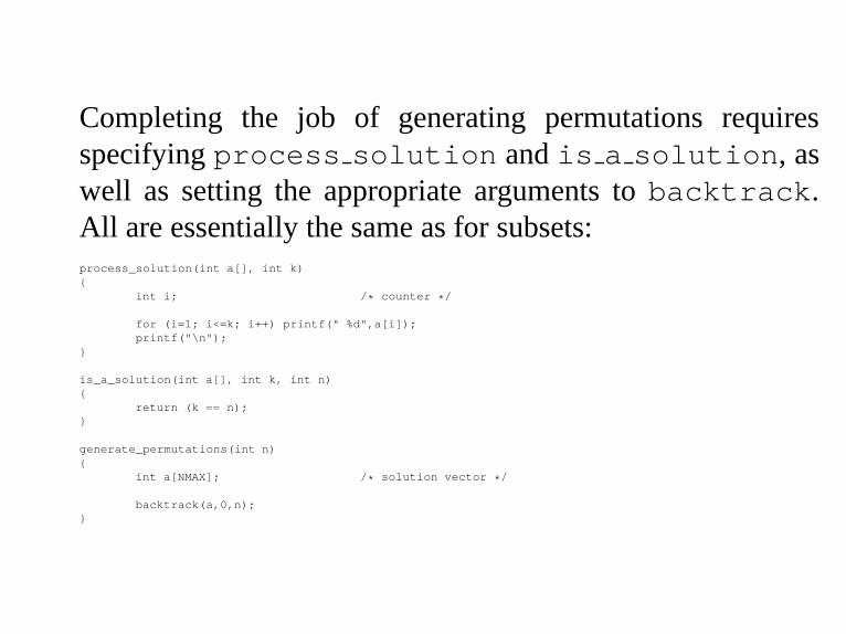
Completing the job of generating permutations requiresspecifyingprocess solution and is a solution, aswell as setting the appropriate arguments tobacktrack.All are essentially the same as for subsets:process_solution(int a[], int k){

int i; /* counter */

for (i=1; i<=k; i++) printf(" %d",a[i]);printf("\n");

}

is_a_solution(int a[], int k, int n){

return (k == n);}

generate_permutations(int n){

int a[NMAX]; /* solution vector */

backtrack(a,0,n);}

The Eight-Queens Problem

The eight queens problem is a classical puzzle of positioningeight queens on an8 × 8 chessboard such that no two queensthreaten each other.Implementing abacktrack search requires us to thinkcarefully about the most concise, efficient way to representour solutions as a vector. What is a reasonable representationfor ann-queens solution, and how big must it be?To make a backtracking program efficient enough to solveinteresting problems, we must prune the search space byterminating every search path the instant it becomes clear itcannot lead to a solution.

Since no two queens can occupy the same column, we knowthat the n columns of a complete solution must form apermutation ofn. By avoiding repetitive elements, we reduceour search space to just8! = 40,320 – clearly short work forany reasonably fast machine.The critical routine is the candidate constructor. Werepeatedly check whether thekth square on the given rowis threatened by any previously positioned queen. If so, wemove on, but if not we include it as a possible candidate:

Implmementation

construct_candidates(int a[], int k, int n, int c[], int *ncandidates){

int i,j; /* counters */bool legal_move; /* might the move be legal? */

*ncandidates = 0;for (i=1; i<=n; i++) {

legal_move = TRUE;for (j=1; j<k; j++) {

if (abs((k)-j) == abs(i-a[j])) /* diagonal threat */legal_move = FALSE;

if (i == a[j]) /* column threat */legal_move = FALSE;

}if (legal_move == TRUE) {

c[*ncandidates] = i;

*ncandidates = *ncandidates + 1;}

}}

The remaining routines are simple, particularly since we areonly interested in counting the solutions, not displaying them:process_solution(int a[], int k){

int i; /* counter */

solution_count ++;}

is_a_solution(int a[], int k, int n){

return (k == n);}

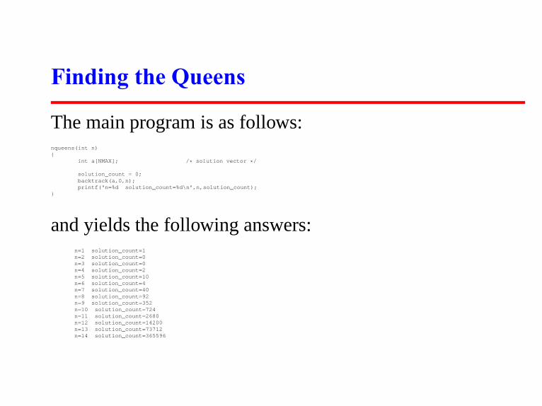
Finding the Queens

The main program is as follows:nqueens(int n){

int a[NMAX]; /* solution vector */

solution_count = 0;backtrack(a,0,n);printf("n=%d solution_count=%d\n",n,solution_count);

}

and yields the following answers:n=1 solution_count=1n=2 solution_count=0n=3 solution_count=0n=4 solution_count=2n=5 solution_count=10n=6 solution_count=4n=7 solution_count=40n=8 solution_count=92n=9 solution_count=352n=10 solution_count=724n=11 solution_count=2680n=12 solution_count=14200n=13 solution_count=73712n=14 solution_count=365596

110801 (Little Bishops)

How many ways can we put downk mutally non-attackingbishops on ann × n board?Can we count the bishops without explicitly constructingevery configuration?

110802 (15-Puzzle Problem)

Can you find a minimum- or near-minimum length path tosolve the 15-puzzle?How do we prune quickly, and how do we eliminateduplicates?

110806 (Garden of Eden)

Given a cellular automata statet and a transition rule, doesthere exist a previous states such thats goes tot?

110807 (Colour Hash)

Does there exist a sequence of moves to reorder the pieces ofthis puzzle?What is the right representation of the puzzle?

Graphs

Graphs are one of the unifying themes of computer science.A graphG = (V, E) is defined by a set ofvertices V , anda set ofedges E consisting of ordered or unordered pairs ofvertices fromV .In modeling a road network, the vertices may represent thecities or junctions, certain pairs of which are connected byroads/edges. In analyzing human interactions, the verticestypically represent people, with edges connecting pairs ofrelated souls.

Flavors of Graphs

The first step in any graph problem is determining whichflavor of graph you are dealing with:

• Undirected vs. Directed – A graph G = (V, E) isundirected if edge (x, y) ∈ E implies that(y, x) is alsoin E.

• Weighted vs. Unweighted – In weighted graphs, eachedge (or vertex) ofG is assigned a numerical value, orweight.

• Cyclic vs. Acyclic – An acyclic graph does not containany cycles.Trees are connected acyclicundirected graphs.

Directed acyclic graphs are calledDAGs.

• Implicit vs. Explicit – Many graphs are not explicitlyconstructed and then traversed, but built as we use them.A good example is in backtrack search.

Data Structures for Graphs

There are several possible ways to represent graphs. SaygraphG = (V, E) containsn vertices andm edges.

• Adjacency Matrix – We can representG using ann × n

matrix M , where elementM [i, j] is, say, 1, if(i, j) is anedge ofG, and 0 if it isn’t. It may use excessive spacefor graphs with many vertices and relatively few edges,however.

• Adjacency Lists in Lists – We can more efficientlyrepresent sparse graphs by using linked lists to store theneighbors adjacent to each vertex. Adjacency lists requirepointers but are not frightening.

• Adjacency Lists in Matrices – Adjacency lists canalso embedded in matrices, thus eliminating the need forpointers. We can represent a list in an array counting howmany elements there are, and packing them into the firstelements of the array. Now we can visit successive theelements from the first to last by incrementing an index ina loop instead of cruising through pointers.

This data structure looks like it combines the worstproperties of adjacency matrices (large space) with theworst properties of adjacency lists (the need to search foredges). However, it is simple to program and understand– and what I will use in my examples.

List in Array Representation

For each graph, we keep count of the number of vertices, andassign each vertex a unique number from 1 tonvertices.The edges go in anMAXV × MAXDEGREE array, so eachvertex can be adjacent toMAXDEGREE others. DefiningMAXDEGREE to beMAXV can be wasteful of space for low-degree graphs:#define MAXV 100 /* maximum number of vertices */#define MAXDEGREE 50 /* maximum vertex outdegree */

typedef struct {int edges[MAXV+1][MAXDEGREE]; /* adjacency info */int degree[MAXV+1]; /* outdegree of each vertex */int nvertices; /* number of vertices in graph */int nedges; /* number of edges in graph */

} graph;

Directed and Undirected Edges

We represent a directed edge(x, y) by the integer y

in x’s adjacency list, which is located in the subarraygraph->edges[x].The degree field counts the number of meaningful entries forthe given vertex.An undirected edge(x, y) appears twice in any adjacency-based graph structure, once asy in x’s list, and once asx iny’s list.

Reading a Graph

A typical graph format consists of an initial line featuringthe number of vertices and edges in the graph, followed bya listing of the edges at one vertex pair per line.read_graph(graph *g, bool directed){

int i; /* counter */int m; /* number of edges */int x, y; /* vertices in edge (x,y) */

initialize_graph(g);scanf("%d %d",&(g->nvertices),&m);for (i=1; i<=m; i++) {

scanf("%d %d",&x,&y);insert_edge(g,x,y,directed);

}}

initialize_graph(graph *g){

int i; /* counter */

g -> nvertices = 0;g -> nedges = 0;for (i=1; i<=MAXV; i++) g->degree[i] = 0;

}

Inserting an Edge

The critical routine isinsert edge. We parameterize itwith a Boolean flagdirected to identify whether we needto insert two copies of each edge or only one. Note the use ofrecursion to solve the problem:insert_edge(graph *g, int x, int y, bool directed){

if (g->degree[x] > MAXDEGREE)printf("Warning: insertion(%d,%d) exceeds max degree\n",x,y);

g->edges[x][g->degree[x]] = y;g->degree[x] ++;

if (directed == FALSE)insert_edge(g,y,x,TRUE);

elseg->nedges ++;

}

Breadth-First Traversal

The basic operation in most graph algorithms is completelyand systematically traversing the graph. We want to visitevery vertex and every edge exactly once in some well-defined order.Breadth-first search is appropriate if we are interested inshortest paths on unweighted graphs.

Discovered vs. Processed Vertices

Our implementationbfs uses two Boolean arrays tomaintain our knowledge about each vertex in the graph.A vertex isdiscovered the first time we visit it. A vertex isconsideredprocessed after we have traversed all outgoingedges from it. Thus each vertex passes from undiscovered todiscovered to processed over the search.Once a vertex is discovered, it is placed on a queue. Sincewe process these vertices in first-in, first-out order, the oldestvertices are expanded first, which are exactly those closest tothe root:

Initializing Search

bool processed[MAXV]; /* which vertices have been processed */bool discovered[MAXV]; /* which vertices have been found */int parent[MAXV]; /* discovery relation */

initialize_search(graph *g){

int i; /* counter */

for (i=1; i<=g->nvertices; i++) {processed[i] = discovered[i] = FALSE;parent[i] = -1;

}}

BFS Implementation

bfs(graph *g, int start){

queue q; /* queue of vertices to visit */int v; /* current vertex */int i; /* counter */

init_queue(&q);enqueue(&q,start);discovered[start] = TRUE;

while (empty(&q) == FALSE) {v = dequeue(&q);process_vertex(v);processed[v] = TRUE;for (i=0; i<g->degree[v]; i++)

if (valid_edge(g->edges[v][i]) == TRUE) {if (discovered[g->edges[v][i]] == FALSE) {

enqueue(&q,g->edges[v][i]);discovered[g->edges[v][i]] = TRUE;parent[g->edges[v][i]] = v;

}if (processed[g->edges[v][i]] == FALSE)

process_edge(v,g->edges[v][i]);}

}}

Exploiting Traversal

The exact behavior ofbfs depends upon the functionsprocess vertex() and process edge(). Throughthese functions, we can easily customize what the traversaldoes as it makes one official visit to each edge and eachvertex. By setting the functions toprocess_vertex(int v){

printf("processed vertex %d\n",v);}

process_edge(int x, int y){

printf("processed edge (%d,%d)\n",x,y);}

we print each vertex and edge exactly once.

Finding Paths

The vertex which discovered vertexi is defined asparent[i]. The parent relation defines a tree of discoverywith the initial search node as the root of the tree.The unique BFS tree path from the root to any nodex ∈ V uses the smallest number of edges (or equivalently,intermediate nodes) possible on any root-to-x path in thegraph.We can reconstruct this path by following the chain ofancestors backwards fromx to the root. We cannot findthe path from the root tox, since that does not follow thedirection of the parent pointers.

Since this is the reverse of how we normally want the path,wecan either (1) store it and then explicitly reverse it using astack, or (2) let recursion reverse it for us, as in the followingslick routine:find_path(int start, int end, int parents[]){

if ((start == end) || (end == -1))printf("\n%d",start);

else {find_path(start,parents[end],parents);printf(" %d",end);

}}

Depth-First Search

Depth-first search uses essentially the same idea as backtrack-ing. Both involve exhaustively searching all possibilities, andbacking up as soon as there is no unexplored possibility forfurther advancement. Both are best understood as recursivealgorithms.Depth-first search can be thought of as breadth-first searchwith a stack instead of a queue. The beauty of implementingdfs recursively is that recursion eliminates the need to keepan explicit stack:

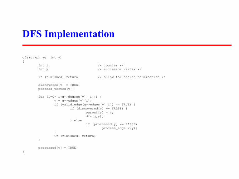
DFS Implementation

dfs(graph *g, int v){

int i; /* counter */int y; /* successor vertex */

if (finished) return; /* allow for search termination */

discovered[v] = TRUE;process_vertex(v);

for (i=0; i<g->degree[v]; i++) {y = g->edges[v][i];if (valid_edge(g->edges[v][i]) == TRUE) {

if (discovered[y] == FALSE) {parent[y] = v;dfs(g,y);

} elseif (processed[y] == FALSE)

process_edge(v,y);}if (finished) return;

}

processed[v] = TRUE;}

Connected Components

The connected components of an undirected graph are theseparate “pieces” of the graph such that there is no connectionbetween the pieces.Many seemingly complicated problems reduce to findingconnected components. Testing whether Rubik’s cube or the15-puzzle can be solved from any position is really askingwhether the graph of legal configurations is connected.Connected components can found using DFS or BFS.Anything we discover during this search must be part of thesame connected component. We then repeat the search fromany undiscovered vertex (if one exists) to define the nextcomponent, until all vertices have been found:

Connected Components Implementation

connected_components(graph *g){

int c; /* component number */int i; /* counter */

initialize_search(g);

c = 0;for (i=1; i<=g->nvertices; i++)

if (discovered[i] == FALSE) {c = c+1;printf("Component %d:",c);dfs(g,i);printf("\n");

}}

Topological Sorting

Topological sorting is the fundamental operation on directedacyclic graphs (DAGs). It constructs an ordering of thevertices such that all directed edges go from left to right.Such an ordering clearly cannot exist if the graph containsany directed cycles, because there is no way you can keepgoing right on a line and still return back to where you startedfrom!

Longest Path in a DAG

The importance of topological sorting is that it gives us a wayto process each vertex before any of its successors.Suppose we seek the shortest (or longest) path fromx toy in aDAG. Certainly no vertex appearing aftery in the topologicalorder can contribute to any such path, because there will beno way to get back toy.We can appropriately process all the vertices from left to rightin topological order, considering the impact of their outgoingedges, and know that we will look at everything we needbefore we need it.

Topological Sorting Algorithms

Topological sorting can be performed using DFS.However, a more straightforward algorithm does an analysisof the in-degrees of each vertex in a DAG. Any in-degree 0vertex may safely be placed first in topological order.Deleting its outgoing edges may create new in-degree 0vertices, continuing the process.compute_indegrees(graph *g, int in[]){

int i,j; /* counters */

for (i=1; i<=g->nvertices; i++) in[i] = 0;

for (i=1; i<=g->nvertices; i++)for (j=0; j<g->degree[i]; j++) in[ g->edges[i][j] ] ++;

}

topsort(graph *g, int sorted[]){

int indegree[MAXV]; /* indegree of each vertex */queue zeroin; /* vertices of indegree 0 */int x, y; /* current and next vertex */int i, j; /* counters */

compute_indegrees(g,indegree);init_queue(&zeroin);for (i=1; i<=g->nvertices; i++)

if (indegree[i] == 0) enqueue(&zeroin,i);

j=0;while (empty(&zeroin) == FALSE) {

j = j+1;x = dequeue(&zeroin);sorted[j] = x;for (i=0; i<g->degree[x]; i++) {

y = g->edges[x][i];indegree[y] --;if (indegree[y] == 0) enqueue(&zeroin,y);

}}

if (j != g->nvertices)printf("Not a DAG -- only %d vertices found\n",j);

}

110902 (Playing with Wheels)

Move from one number to another number using a minimumnumber of steps, while avoiding forbidden states.What is the graph, and is it weighted or unweighted?

110903 (The Tourist Guide)

Minimize the number of trips a guide needs to make in orderto ferry a group of tourists from one place to another.What is the graph theoretic problem being solved here?

110906 (Tower of Cubes)

Build the tallest possible of cubes such that touching facecolors match and lighter cubes are always on top of heaviercubes.What is the graph, and is it directed or undirected?

110907 (From Dusk Till Dawn)

Find the shortest train trip between two different cities subjectto a vampire’s particular constraints.What is the graph, and is it weighted or unweighted?

Properties of Graphs

Graph theory is the study of the properties of graphstructures. It provides us with a language with which to talkabout graphs.The key to solving many problems is identifying thefundamental graph-theoretic notion underlying the situationand then using classical algorithms to solve the resultingproblem.

Connectivity

A graph isconnectedif there is an undirected path betweenevery pair of vertices.The existence of a spanning tree is sufficient to proveconnectivity. A breadth-first or depth-first search-basedconnected components algorithm can be used to find such aspanning tree.However, there are other notions of connectivity. The mostinteresting special case when there is a single weak link in thegraph. A single vertex whose deletion disconnects the graphis called anarticulation vertex; any graph without such avertex is said to bebiconnected. A single edge whose deletiondisconnects the graph is called abridge.

Testing for articulation vertices or bridges is easy via bruteforce. For each vertex/edge, delete it from the graph and testwhether the resulting graph remains connected. Be sure toadd that vertex/edge back before doing the next deletion!In directed graphs we are often concerned withstronglyconnected components, that is, partitioning the graph intochunks such that there are directed paths between all pairsof vertices within a given chunk. Road networks should bestrongly connected, or else there will be places you can driveto but not drive home from without violating one-way signs.

Cycles in Graphs

All non-tree connected graphs contain cycles.An Eulerian cycleis a tour which visits every edge of thegraph exactly once. A mailman’s route is ideally an Euleriancycle, so he can visit every street (edge) in the neighborhoodonce before returning home.An undirected graph contains an Eulerian cycle if it isconnected and every vertex is of even degree. Why?The circuit must enter and exit every vertex it encounters,implying that all degrees must be even.

Finding an Eulerian Cycle

We can find an Eulerian cycle by building it one cycle at atime. We can find a simple cycle in the graph by finding aback edge using DFS. Deleting the edges on this cycle leaveseach vertex with even degree. Once we have partitioned theedges into edge-disjoint cycles, we can merge these cyclesarbitrarily at common vertices to build an Eulerian cycle.A Hamiltonian cycleis a tour which visits every vertex of thegraph exactly once. The traveling salesman problem asks forthe shortest such tour on a weighted graph.Unfortunately, no efficient algorithm exists for solvingHamiltonian cycle problems. If the graph is sufficientlysmall, it can be solved via backtracking.

Minimum Spanning Trees

A spanning treeof a graphG = (V, E) is a subset of edgesfrom E forming a tree connecting all vertices ofV .For edge-weighted graphs, we are particularly interested intheminimum spanning tree, the spanning tree whose sum ofedge weights is the smallest possible.Minimum spanning trees are the answer whenever we need toconnect a set of points (representing cities, junctions, or otherlocations) by the smallest amount of roadway, wire, or pipe.We present Prim’s algorithm because it is simpler to program,and because it gives Dijkstra’s shortest path algorithm withvery minimal changes.

Representing Weighted Graphs

We generalize the graph data structure to support edge-weighted graphs. Each edge-entry previously contained onlythe other endpoint of the given edge. We must replace this bya record allowing us to annotate the edge with weights:typedef struct {

int v; /* neighboring vertex */int weight; /* edge weight */

} edge;

typedef struct {edge edges[MAXV+1][MAXDEGREE]; /* adjacency info */int degree[MAXV+1]; /* outdegree of vertex */int nvertices; /* number of vertices */int nedges; /* number of edges in graph */

} graph;

Prim’s Algorithm

Prim’s algorithm grows the minimum spanning tree in stagesstarting from a given vertex. At each iteration, we add onenew vertex into the spanning tree. We greedily add thelowest-weight edge linking a vertex in the tree to a vertexon the outside.Our implementation keeps track of the cheapest edge fromthe tree to every non-tree vertex in the graph. The cheapestedge over all remaining non-tree vertices gets added in eachiteration.We must update the costs of getting to the non-tree verticesafter each insertion.

Prim’s Implementation

prim(graph *g, int start) {int i,j; /* counters */bool intree[MAXV]; /* is vertex in the tree yet? */int distance[MAXV]; /* vertex distance from start */int v; /* current vertex to process */int w; /* candidate next vertex */int weight; /* edge weight */int dist; /* shortest current distance */

for (i=1; i<=g->nvertices; i++) {intree[i] = FALSE;distance[i] = MAXINT;parent[i] = -1;

}distance[start] = 0;v = start;

while (intree[v] == FALSE) {intree[v] = TRUE;for (i=0; i<g->degree[v]; i++) {

w = g->edges[v][i].v;weight = g->edges[v][i].weight;if ((distance[w] > weight) && (intree[w]==FALSE)) {

distance[w] = weight;parent[w] = v;

}}

v = 1;dist = MAXINT;for (i=2; i<=g->nvertices; i++)

if ((intree[i]==FALSE) && (dist > distance[i])) {dist = distance[i];

v = i;}

}}

Dijkstra’s Algorithm for Shortest Paths

BFS doesnot suffice for finding shortest paths in weightedgraphs, because the shortest weighted path froma to b doesnot necessarily contain the fewest number of edges.Dijkstra’s algorithm is the method of choice for finding theshortest path between two vertices in an edge- and/or vertex-weighted graph. It finds the shortest path from start vertexs

to every other vertex, including your desired destinationt.The basic idea is very similar to Prim’s algorithm. In eachiteration, we are going to add exactly one vertex to the tree ofvertices for which weknowthe shortest path froms.

The difference between Dijkstra’s and Prim’s algorithms ishow they rate the desirability of each outside vertex. Inshortest path, we want to include the outside vertex whichis closest (in shortest-path distance) to the start. This is afunction of both the new edge weightand the distance fromthe start of the tree-vertex it is adjacent to.In fact, this change is very minor. Below we give animplementation of Dijkstra’s algorithm based on changingexactly three lines from our Prim’s implementation – one ofwhich is simply the name of the function!Unlike Prim’s, Dijkstra’s algorithm only works on graphswithout negative-cost edges. But most applications do notfeature negative-weight edges. . .

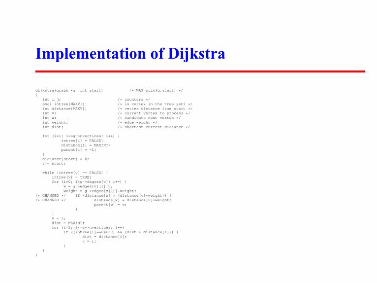
Implementation of Dijkstra

dijkstra(graph *g, int start) /* WAS prim(g,start) */{

int i,j; /* counters */bool intree[MAXV]; /* is vertex in the tree yet? */int distance[MAXV]; /* vertex distance from start */int v; /* current vertex to process */int w; /* candidate next vertex */int weight; /* edge weight */int dist; /* shortest current distance */

for (i=1; i<=g->nvertices; i++) {intree[i] = FALSE;distance[i] = MAXINT;parent[i] = -1;

}distance[start] = 0;v = start;

while (intree[v] == FALSE) {intree[v] = TRUE;for (i=0; i<g->degree[v]; i++) {

w = g->edges[v][i].v;weight = g->edges[v][i].weight;

/* CHANGED */ if (distance[w] > (distance[v]+weight)) {/* CHANGED */ distance[w] = distance[v]+weight;

parent[w] = v;}

}v = 1;dist = MAXINT;for (i=2; i<=g->nvertices; i++)

if ((intree[i]==FALSE) && (dist > distance[i])) {dist = distance[i];v = i;

}}

}

All-Pairs Shortest Path

Many applications need to know the length of the shortestpath between all pairs of vertices in a given graph. Forexample, suppose you want to find the “center” vertex, theone which minimizes the longest or average distance to allthe other nodes. This might be the best place to start a newbusiness.We could solve this problem by calling Dijkstra’s algorithmfrom each of then possible starting vertices. But Floyd’sall-pairs shortest-path algorithm is an amazingly slick way toconstruct this distance matrix from the original weight matrixof the graph.

Floyd’s Algorithm

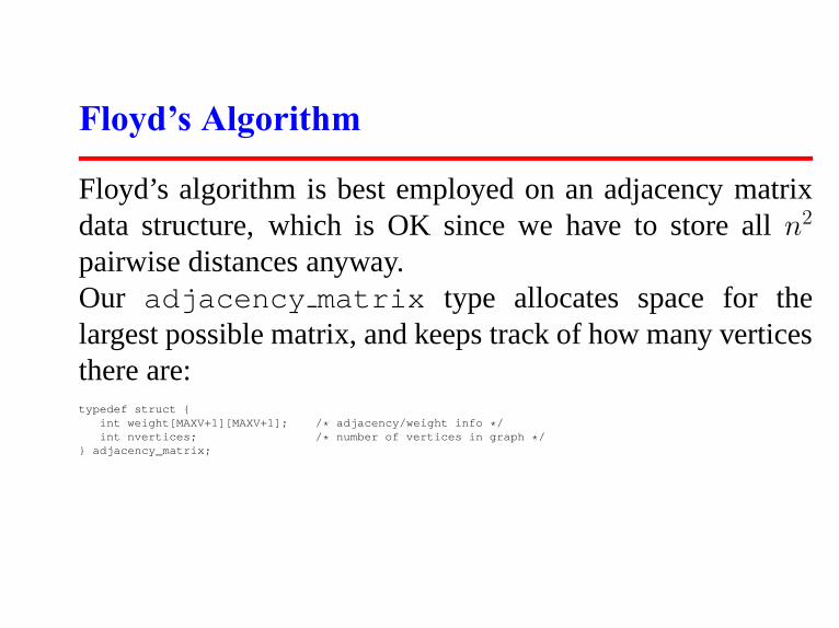
Floyd’s algorithm is best employed on an adjacency matrixdata structure, which is OK since we have to store alln2

pairwise distances anyway.Our adjacency matrix type allocates space for thelargest possible matrix, and keeps track of how many verticesthere are:typedef struct {

int weight[MAXV+1][MAXV+1]; /* adjacency/weight info */int nvertices; /* number of vertices in graph */

} adjacency_matrix;

Initializing the Adjacency MatrixA critical issue in any adjacency matrix implementation ishow we denote the edges which are not present in the graph.For unweighted graphs, a common convention is that graphedges are denoted by1 and non-edges by0.This gives exactly the wrong interpretation if the numbersdenote edge weights, for the non-edges get interpreted as afree ride between vertices. Instead, we should initialize eachnon-edge toMAXINT.initialize_adjacency_matrix(adjacency_matrix *g){

int i,j; /* counters */

g -> nvertices = 0;

for (i=1; i<=MAXV; i++)for (j=1; j<=MAXV; j++)

g->weight[i][j] = MAXINT;}

Floyd’s Idea

Floyd’s algorithm numbers the vertices ofG from 1 to n,using these numbers not to label the vertices but to orderthem.We will perform n iterations, where thekth iteration allowsonly the firstk vertices as possible intermediate steps on thepath between each pair of verticesx andy.Allowing thekth vertex as a new possible intermediary helpsiff there is a short path that goes throughk, so

W [i, j]k

= min(W [i, j]k−1, W [i, k]

k−1+ W [k, j]

k−1)

Implementation of Floyd’s Algorithm

The correctness of this is somewhat subtle, and we encourageyou to convince yourself of it. But there is nothing subtleabout how short and sweet the implementation is:floyd(adjacency_matrix *g){

int i,j; /* dimension counters */int k; /* intermediate vertex counter */int through_k; /* distance through vertex k */

for (k=1; k<=g->nvertices; k++)for (i=1; i<=g->nvertices; i++)

for (j=1; j<=g->nvertices; j++) {through_k = g->weight[i][k]+g->weight[k][j];if (through_k < g->weight[i][j])

g->weight[i][j] = through_k;}

}

Transitive Closure

Floyd’s algorithm has another important application, that ofcomputing thetransitive closureof a directed graph. Inanalyzing a directed graph, we are often interested in whichvertices are reachable from a given node.For example, consider theblackmail graphdefined on a setof n people, where there is a directed edge(i, j) if i hassensitive-enough private information onj so thati can gethim to do whatever he wants. You wish to hire one of thesen

people to be your personal representative. Who has the mostpower in terms of blackmail potential?

A simplistic answer would be the vertex of highest degree.But Steve might only be able to blackmail Miguel directly,but if Miguel can blackmail everyone else then Steve is theman you want to hire.The vertices reachable from any single node can be computedusing using breadth-first or depth-first search. But the wholebatch can be computed as an all-pairs shortest-path problem.If the shortest path fromi to j remainsMAXINT after runningFloyd’s algorithm, you can be sure there is no directed pathfrom i to j.

Network Flow

Any edge-weighted graph can be thought of as a network ofpipes, where the weight of edge(i, j) measures thecapacityof the pipe. For a given weighted graphG and two verticess and t, the network flow problemasks for the maximumamount of flow which can be sent froms to t while respectingthe maximum capacities of each pipe.While the network flow problem is of independent interest,its primary importance is that of being able to solve otherimportant graph problems. Classic examples are bipartitematching and edge/vertex connectivity testing.

Bipartite Graphs

GraphG is bipartite or two-colorableif the vertices can bedivided into two sets, say,L andR, such that all edges inGhave one vertex inL and one vertex inR.Many naturally defined graphs are bipartite. For example,suppose certain vertices represent jobs to be done and theremaining vertices people who can potentially do them. Theexistence of edge(j, p) means that jobj can potentially doneby personp. Or let certain vertices represent boys and certainvertices girls, with edges representing compatible pairs.

Bipartite Matching

A matching in a graphG = (V, E) is a subset of edgesE ′ ⊂ E such that no two edges inE ′ share a vertex. Thusa matching pairs off certain vertices such that every vertex isin at most one such pair.Matchings in bipartitie graphs have natural interpretations asjob assignments or as marriages.The largest possible bipartite matching can be found usingnetwork flow. The maximum weighted bipartite matching canbe found using the Hungarian algorithm. See the textbook fordetails.

111001 (Freckles)

Connect the dots using as little ink as possible.What classical graph problem does this correspond to?

111002 (The Necklace)

Does there exist a way to lace up bicolored beads so that eachpair of neighboring bead-faces share a color?What classical graph problem does this correspond to?What efficiently computedclassical graph problem does thisalso correspond to?

111006 (Tourist Guide)

What vertices in the graph separate the graph into two pieces,i.e. all paths betweena andb must go through them for anyaandb?How can we efficiently test whetherv is such a vertex?

111007 (The Grand Dinner)

Match team members to tables so that no two team memberssit at the same table.Can this be done using bipartite matching/network flow?

Dynamic Programming

Dynamic programming is a very powerful, general tool forsolving optimization problems on left-right-ordered itemssuch as character strings. Once understood it is relatively easyto apply, but many people have trouble understanding it.Start by reviewing the binomial coefficient function in thecombinatorics section, as an example of how we stored partialresults to help us compute what we were looking for.Floyd’s all-pairs shortest-path algorithm discussed in thegraph algorithms chapter is another example of dynamicprogramming.

Greedy Algorithms

Greedyalgorithms focus on making the best local choice ateach decision point. For example, a natural way to compute ashortest path fromx to y might be to walk out ofx, repeatedlyfollowing the cheapest edge until we get toy. Natural, butwrong!In the absence of a correctness proof greedy algorithms arevery likely to fail.Dynamic programming gives us a way to design customalgorithms which systematically search all possibilities (thusguaranteeing correctness) while storing results to avoidrecomputing (thus providing efficiency).

Evaluating Recurrence Relations

Dynamic programming algorithms are defined by recursivealgorithms/functions that describe the solution to the entireproblem in terms of solutions to smaller problems. Back-tracking is one such recursive procedure we have seen, as isdepth-first search in graphs.Efficiency in any such recursive algorithm requires storingenough information to avoid repeating computations we havedone before. Depth-first search in graphs is efficient becausewe mark the vertices we have visited so we don’t visit themagain.

Dynamic programming is a technique for efficiently imple-menting a recursive algorithm by storing partial results. Thetrick is to see that the naive recursive algorithm repeatedlycomputes the same subproblems over and over and overagain. If so, storing the answers to them in a table insteadof recomputing can lead to an efficient algorithm.Thus we must first hunt for a correct recursive algorithm –later we can worry about speeding it up by using a resultsmatrix.

Edit DistanceMisspellings and changes in word usage (“Thou shaltnot kill” morphs into “You should not murder.”) makeapproximate pattern matchingan important problem.A reasonable distance measure minimizes the cost of thechangeswhich have to be made to convert one string toanother.There are three natural types of changes:

• Substitution – Change a single character from patterns

to a different character in textt, such as changing “shot”to “spot”.

• Insertion – Insert a single character into patterns to helpit match textt, such as changing “ago” to “agog”.

• Deletion – Delete a single character from patterns tohelp it match textt, such as changing “hour” to “our”.

Properly posing the question of string similarity requires usto set the cost of each of these string transform operations.Setting each operation to cost one step defines theeditdistancebetween two strings.

Recursive Algorithm

We can compute the edit distance with recursive algorithmusing the observation that the last character in the string musteither be matched, substituted, inserted, or deleted.If weknew the cost of editing the three pairs of smaller strings,we could decide which option leads to the best solutionand choose that option accordingly. Wecan learn this cost,through the magic of recursion:

#define MATCH 0 /* enumerated type symbol for match */#define INSERT 1 /* enumerated type symbol for insert */#define DELETE 2 /* enumerated type symbol for delete */

int string_compare(char *s, char *t, int i, int j){

int k; /* counter */int opt[3]; /* cost of the three options */int lowest_cost; /* lowest cost */

if (i == 0) return(j * indel(’ ’));if (j == 0) return(i * indel(’ ’));

opt[MATCH] = string_compare(s,t,i-1,j-1) + match(s[i],t[j]);opt[INSERT] = string_compare(s,t,i,j-1) + indel(t[j]);opt[DELETE] = string_compare(s,t,i-1,j) + indel(s[i]);

lowest_cost = opt[MATCH];for (k=INSERT; k<=DELETE; k++)

if (opt[k] < lowest_cost) lowest_cost = opt[k];

return( lowest_cost );}

Speeding it Up

This program is absolutely correct but impossibly slow tocompare two 12-character strings! It takes exponential timebecause it recomputes values again and again.But there can only be|s| · |t| possible unique recursive calls,since there are only that many distinct(i, j) pairs to serve asthe parameters of recursive calls. By storing the values foreach of these(i, j) pairs in a table, we can just look them upas needed.The table is a two-dimensional matrixm where each of the|s| · |t| cells contains the cost of the optimal solution of thissubproblem, as well as a parent pointer explaining how wegot to this location:

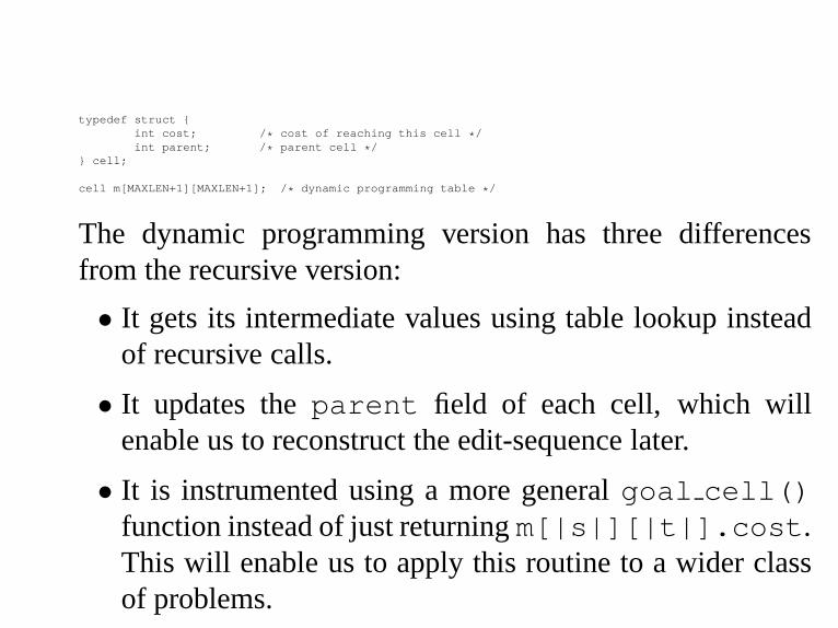
typedef struct {int cost; /* cost of reaching this cell */int parent; /* parent cell */

} cell;

cell m[MAXLEN+1][MAXLEN+1]; /* dynamic programming table */

The dynamic programming version has three differencesfrom the recursive version:

• It gets its intermediate values using table lookup insteadof recursive calls.

• It updates theparent field of each cell, which willenable us to reconstruct the edit-sequence later.

• It is instrumented using a more generalgoal cell()function instead of just returningm[|s|][|t|].cost.This will enable us to apply this routine to a wider classof problems.

Be aware that we adhere to certain unusual string and indexconventions in the following routines. In particular, weassume that each string has been padded with an initial blankcharacter, so the first real character of strings sits ins[1].

int string_compare(char *s, char *t){

int i,j,k; /* counters */int opt[3]; /* cost of the three options */

for (i=0; i<MAXLEN; i++) {row_init(i);column_init(i);

}

for (i=1; i<strlen(s); i++)for (j=1; j<strlen(t); j++) {

opt[MATCH] = m[i-1][j-1].cost + match(s[i],t[j]);opt[INSERT] = m[i][j-1].cost + indel(t[j]);opt[DELETE] = m[i-1][j].cost + indel(s[i]);

m[i][j].cost = opt[MATCH];m[i][j].parent = MATCH;for (k=INSERT; k<=DELETE; k++)

if (opt[k] < m[i][j].cost) {m[i][j].cost = opt[k];m[i][j].parent = k;

}}

goal_cell(s,t,&i,&j);return( m[i][j].cost );

}

Example

To determine the value of cell(i, j) we need three valuessitting and waiting for us, namely, the cells(i − 1, j − 1),(i, j − 1), and (i − 1, j). Any evaluation order with thisproperty will do, including row-major order.“thou shalt not” goes to “you should not” in 5 moves:DSMMMMMISMSMMMM

y o u - s h o u l d - n o t: 0 1 2 3 4 5 6 7 8 9 10 11 12 13 14

t: 1 1 2 3 4 5 6 7 8 9 10 11 12 13 13h: 2 2 2 3 4 5 5 6 7 8 9 10 11 12 13o: 3 3 2 3 4 5 6 5 6 7 8 9 10 11 12u: 4 4 3 2 3 4 5 6 5 6 7 8 9 10 11-: 5 5 4 3 2 3 4 5 6 6 7 7 8 9 10s: 6 6 5 4 3 2 3 4 5 6 7 8 8 9 10h: 7 7 6 5 4 3 2 3 4 5 6 7 8 9 10a: 8 8 7 6 5 4 3 3 4 5 6 7 8 9 10l: 9 9 8 7 6 5 4 4 4 4 5 6 7 8 9t: 10 10 9 8 7 6 5 5 5 5 5 6 7 8 8-: 11 11 10 9 8 7 6 6 6 6 6 5 6 7 8n: 12 12 11 10 9 8 7 7 7 7 7 6 5 6 7o: 13 13 12 11 10 9 8 7 8 8 8 7 6 5 6t: 14 14 13 12 11 10 9 8 8 9 9 8 7 6 5

Reconstructing the Path

The possible solutions are described by paths throughthe dynamic programming matrix, starting from the initialconfiguration(0, 0) to the final goal state(|s|, |t|).Reconstructing these decisions is done by walking backwardfrom the goal state, following theparent pointer to anearlier cell. Theparent field for m[i,j] tells us whetherthe transform at(i, j) wasMATCH, INSERT, orDELETE.

Walking backward reconstructs the solution in reverse order.However, clever use of recursion can do the reversing for us:reconstruct_path(char *s, char *t, int i, int j){

if (m[i][j].parent == -1) return;

if (m[i][j].parent == MATCH) {reconstruct_path(s,t,i-1,j-1);match_out(s, t, i, j);return;

}if (m[i][j].parent == INSERT) {

reconstruct_path(s,t,i,j-1);insert_out(t,j);return;

}if (m[i][j].parent == DELETE) {

reconstruct_path(s,t,i-1,j);delete_out(s,i);return;

}}

Customizing Edit Distance

• Table Initialization – The functionsrow init() andcolumn init() initialize the zeroth row and columnof the dynamic programming table, respectively.

• Penalty Costs – The functionsmatch(c,d) andindel(c) present the costs for transforming characterc to d and inserting/deleting characterc. For standard editdistance,match costs 0 for matching characters, and 1otherwise, whileindel returns 1.

• Goal Cell Identification – The functiongoal cellreturns the indices of the cell marking the endpoint of the

solution. For edit distance, this is defined by the length ofthe two input strings.

• Traceback Actions – The functionsmatch out,insert out, anddelete out perform the appropri-ate actions for each edit-operation during traceback. Foredit distance, this might mean printing out the name ofthe operation or character involved, as determined by theneeds of the application.

Substring Matching

Suppose that we want to find where a short patterns bestoccurs within a long textt, say, searching for “Skiena” in allits misspellings (Skienna, Skena, Skina, . . . ).We want an edit distance search where the cost of startingthe match is independent of the position in the text, so that amatch in the middle is not prejudiced against.Likewise, the goal state is not necessarily at the end of bothstrings, but the cheapest place to match the entire patternsomewhere in the text. Modifying these two functions givesus the correct solution:

row_init(int i){

m[0][i].cost = 0; /* note change */m[0][i].parent = -1; /* note change */

}

goal_cell(char *s, char *t, int *i, int *j){

int k; /* counter */

*i = strlen(s) - 1;

*j = 0;for (k=1; k<strlen(t); k++)

if (m[*i][k].cost < m[*i][*j].cost) *j = k;}

Longest Common Subsequence

Often we are interested in finding the longest scattered stringof characters which is included within both words. Thelongest common subsequence(LCS) between “democrat” and“republican” iseca.A common subsequence is defined by identical-charactermatches in an edit trace. To maximize such traces, we mustprevent substitution of non-identical characters by changingthe match-cost function:int match(char c, char d){

if (c == d) return(0);else return(MAXLEN);

}

Maximum Monotone Subsequence

A numerical sequence ismonotonically increasingif the ithelement is at least as big as the(i − 1)st element. Themaximum monotone subsequenceproblem seeks to delete thefewest number of elements from an input stringS to leavea monotonically increasing subsequence. Thus a longestincreasing subsequence of “243517698” is “23568.”In fact, this is just a longest common subsequence problem,where the second string is the elements ofS sorted inincreasing order.The trick to using edit distance is observing that your problemis just a special case of approximate string matching.

111101 (Is Bigger Smarter?)

Find the longest sequence of elephants whose weights areincreasing but whose IQ’s are decreasing.Can this be done as a special case of edit distance?

111103 (Weights and Measures)

Find the tallest possible stack of turtles you can build, whereeach turtle has a strength and weight.Can this be done as a special case of edit distance?

111104 (Unidirectional TSP)

Find the cheapest left-right path across a matrix.Is this shortest path or dynamic programming, or is Dijkstra’salgorithm really dynamic programming?

111106 (Ferry Loading)

How can we fit the most amount of cars on a two-lane ferry?Does always putting the next car on the side with the mostremaining room solve the problem?Can we exploit the fact that the sum of accumulated carlengths on each lane of the ferry is always an integer?

Geometry

This chapter will deal with programming problems associatedwith “real” geometry – lines, points, circles, and so forth.Although you did geometry in high school, it can besurprisingly difficult to program even very simple things. Onereason is that floating point arithmetic introduces numericaluncertainty.Another difficulty of geometric programming is that certain“obvious” operations you do with a pencil, such as finding theintersection of two lines, requires non-trivial programming todo correctly with a computer.

Degeneracy

Special cases ordegeneracies require extra attention whendoing geometric programming. For these reasons I recom-mend you carefully study my code fragments before writingyour own.There is more geometry to come next week, when we con-sider problems associated with line segments and polygons afield known ascomputational geometry,

Lines

Straight lines are the shortest distance between any twopoints. Lines are of infinite length in both directions, asopposed toline segments, which are finite. We limit ourdiscussion here to lines in the plane.Every line l is completely represented by any pair of points(x1, y1) and(x2, y2) which lie on it.Lines are also completely described by equations such asy = mx + b, wherem is the slope of the line andb is they-intercept, i.e., the unique point(0, b) where it crosses thex-axis.

Line Type

Vertical lines cannot be described by such equations, how-ever, because dividing by∆x means dividing by zero. Theequationx = c denotes a vertical line that crosses thex-axisat the point(c, 0).We use the more general formulaax + by + c = 0 as thefoundation of our line type because it covers all possible linesin the plane:typedef struct {

double a; /* x-coefficient */double b; /* y-coefficient */double c; /* constant term */

} line;

Multiplying these coefficients by any non-zero constantyields an alternate representation for any line. We establisha canonical representation by insisting that they-coefficientequal 1 if it is non-zero. Otherwise, we set thex-coefficientto 1:points_to_line(point p1, point p2, line *l){

if (p1[X] == p2[X]) {l->a = 1;l->b = 0;l->c = -p1[X];

} else {l->b = 1;l->a = -(p1[Y]-p2[Y])/(p1[X]-p2[X]);l->c = -(l->a * p1[X]) - (l->b * p1[Y]);

}}

point_and_slope_to_line(point p, double m, line *l){

l->a = -m;l->b = 1;l->c = -((l->a*p[X]) + (l->b*p[Y]));

}

Line Intersection

Two distinct lines have oneintersection point unless they areparallel; in which case they have none. Parallel lines sharethe same slope but have different intercepts and by definitionnever cross.bool parallelQ(line l1, line l2){

return ( (fabs(l1.a-l2.a) <= EPSILON) &&(fabs(l1.b-l2.b) <= EPSILON) );

}

The intersection point of linesl1 : y = m1x + b1 andl2 : y2 =

m2x + b2 is the point where they are equal, namely,

x =b2 − b1

m1 − m2

, y = m1

b2 − b1

m1 − m2

+ b1

Implementation

intersection_point(line l1, line l2, point p){

if (same_lineQ(l1,l2)) {printf("Warning: Identical lines, all points intersect.\n");p[X] = p[Y] = 0.0;return;

}

if (parallelQ(l1,l2) == TRUE) {printf("Error: Distinct parallel lines do not intersect.\n");return;

}

p[X] = (l2.b*l1.c - l1.b*l2.c) / (l2.a*l1.b - l1.a*l2.b);

if (fabs(l1.b) > EPSILON) /* test for vertical line */p[Y] = - (l1.a * (p[X]) + l1.c) / l1.b;

elsep[Y] = - (l2.a * (p[X]) + l2.c) / l2.b;

}

Angles

An angle is the union of two rays sharing a common endpoint.The entire range of angles spans from0 to 2π radians or,equivalently,0 to 360 degrees. Most trigonometric librariesassume angles are measured in radians.A right angle measures90

o or π/2 radians.Any two non-parallel lines intersect each other at a givenangle. Linesl1 : a1x+b1y+c1 = 0 andl2 : a2x+b2y+c2 = 0,written in the general form, intersect at the angleθ given by:

tan θ =a1b2 − a2b1

a1a2 + b1b2

For lines in slope-intercept form this reduces totan θ =

(m2 − m1)/(m1m2 + 1).Two lines areperpendicular if they cross at right angles toeach other. The line perpendicular tol : y = mx + b isy = (−1/m)x + b′, for all values ofb′.

Closest Point

A very useful subproblem is identifying the point on linelwhich is closest to a given pointp. This closest point lies onthe line throughp which is perpendicular tol, and hence canbe found using the routines we have already developed:closest_point(point p_in, line l, point p_c){

line perp; /* perpendicular to l through (x,y) */

if (fabs(l.b) <= EPSILON) { /* vertical line */p_c[X] = -(l.c);p_c[Y] = p_in[Y];return;

}

if (fabs(l.a) <= EPSILON) { /* horizontal line */p_c[X] = p_in[X];p_c[Y] = -(l.c);return;

}

point_and_slope_to_line(p_in,1/l.a,&perp); /* normal case */intersection_point(l,perp,p_c);

}

Triangles

Each pair of rays with a common endpoint defines aninternalangle of a radians and anexternal angle of 2π − a radians.The three internal (smaller) angles of any triangle add up to180

o= π radians.

The Pythagorean theorem enables us to calculate the lengthof the third side of anyright triangle given the length of theother two. Specifically,|a|2 + |b|2 = |c|2, wherea andb arethe two shorter sides, andc is the longest side orhypotenuse.We can go farther to analyze triangles using trigonometry.

TrigonometryThe trigonometric functionssine andcosine are defined as thex- andy-coordinates of points on the unit circle centered at(0, 0). Thetangent is the ratio of sine over cosine.These functions enable us to relate the lengths of any twosides of a right triangleT with the non-right angles ofT . Thenon-hypotenuse edges can be labeled asopposite or adjacentedges in relation to a given anglea. Then

cos(a) =|adjacent|

|hypotenuse|, sin(a) =

|opposite||hypotenuse|

, tan(a) =|opposite|adjacent

Use the famous Indian Chief Soh-Cah-Toa to rememberthese relations. “Cah” meansCosine equalsAdjacent overHypotenuse, for example.

Solving Triangles

TheLaw of Sines provides the relationship between sides andangles in any triangle. For anglesA, B, C, and opposingedgesa, b, c

a

sin A=

b

sin B=

c

sin CThe Law of Cosines is a generalization of the Pythagoreantheorem beyond right angles. For any triangle with anglesA,B, C, and opposing edgesa, b, c,

a2= b2

+ c2− 2bc cos A

Solving triangles is the art of deriving the unknown anglesand edge lengths of a triangle given a subset of suchmeasurements.

Area of a Triangle

The areaA(T ) of a triangleT is given byA(T ) = (1/2)ab,wherea is the altitude andb is the base of the triangle.Another approach to computing the area of a triangle isdirectly from its coordinate representation. Using linearalgebra and determinants, it can be shown that thesigned areaA(T ) of triangleT = (a, b, c) is

2·A(T ) =

∣∣∣∣∣∣∣∣∣∣∣∣

ax ay 1

bx by 1

cx cy 1

∣∣∣∣∣∣∣∣∣∣∣∣

= axby−aybx+aycx−axcy+bxcy−cxby

This formula generalizes nicely to computed! times thevolume of a simplex ind dimensions.

Note that the signed areas can be negative, so we must takethe absolute value to compute the actual area. The signof this area can be used to build important primitives forcomputational geometry.double signed_triangle_area(point a, point b, point c){

return( (a[X]*b[Y] - a[Y]*b[X] + a[Y]*c[X]- a[X]*c[Y] + b[X]*c[Y] - c[X]*b[Y]) / 2.0 );

}

double triangle_area(point a, point b, point c){

return( fabs(signed_triangle_area(a,b,c)) );}

Circles

A circle is defined as the set of points at a given distance (orradius) from its center, (xc, yc). A circle can be representedin two basic ways, either as triples of boundary points orby its center/radius. For most applications, the center/radiusrepresentation is most convenient:typedef struct {

point c; /* center of circle */double r; /* radius of circle */

} circle;

The equation of a circle of radiusr follows directly from itscenter/radius representation,r =

√(x − xc)

2 + (y − yc)2.

Many important quantities associated with circles are easy tocompute. Specifically,A = πr2 andC = 2πr.

A tangent line l intersects the boundary ofc but not itsinterior. The point of contact betweenc andl lies on the lineperpendicular tol through the center ofc.We can compute the unknown tangent lengthx using thePythagorean theorem. Fromx, we can compute either thetangent point or the anglea. The distanced from O to thecenter is computed using the distance formula.Two circlesc1 andc2 of distinct radiir1 andr2 will intersectif and only if the distance between their centers is at mostr1 + r2.The points of intersection form triangles with the two centerswhose edge lengths are totally determined (r1, r2, and thedistance between the centers), so the angles and coordinatescan be computed as needed.

111301 (Dog and Gopher)

Find a hole for a slow gopher to hide from a fast dog.Is the closest holereally the safest spot for the gopher?

111302 (Rope Crisis in Ropeland!)

What is the length of the shortest rope between two pointsaround a circular post?

111305 (Birthday Cake)

How do you cut a circular cake such that both pieces are thesame areaand contain the same number of cherries?There is always a solution to this problem if we remove theconstraint that the cutline have integer coordinates – can youprove it?Is there a more efficient solution than trying all possibleA, Bpairs?

111308 (How Big Is It?)

What is the tightest way to order a non-overlapping collectionof circles so as to minimize the ‘shadow’ of them?Is it better to order the circles from largest to smallest, or tointerleave them?Does the order evernot matter?Will backtracking work for this problem?

Line Segments

Arbitrary closed curves or shapes can be represented byordered collections of line segments orpolygons.A line segment s is the portion of a linel which lies betweentwo given points inclusive. Thus line segments are mostnaturally represented by pairs of endpoints:typedef struct {

point p1,p2; /* endpoints of line segment */} segment;

The most important geometric primitive on segments, testingwhether a given pair of them intersect, proves surprisinglycomplicated because of tricky special cases that arise.

Dealing with Degeneracy

The right way to deal with degeneracy is to base allcomputation on a small number of carefully crafted geometricprimitives. Previously we implemented a general line datatype that successfully dealt with vertical lines; those ofinfinite slope. We can reap the benefits by generalizing ourline intersection routines to line segments.Segment intersection can also be cleanly tested using aprimitive to check whether three ordered points turn in acounterclockwise direction.

Testing Intersectionbool segments_intersect(segment s1, segment s2){

line l1,l2; /* lines containing the input segments */point p; /* intersection point */

points_to_line(s1.p1,s1.p2,&l1);points_to_line(s2.p1,s2.p2,&l2);

if (same_lineQ(l1,l2)) /* overlapping or disjoint segments */return( point_in_box(s1.p1,s2.p1,s2.p2) ||

point_in_box(s1.p2,s2.p1,s2.p2) ||point_in_box(s2.p1,s1.p1,s1.p2) ||point_in_box(s2.p1,s1.p1,s1.p2) );

if (parallelQ(l1,l2)) return(FALSE);

intersection_point(l1,l2,p);

return(point_in_box(p,s1.p1,s1.p2) && point_in_box(p,s2.p1,s2.p2));}

bool point_in_box(point p, point b1, point b2){

return( (p[X] >= min(b1[X],b2[X])) && (p[X] <= max(b1[X],b2[X]))&& (p[Y] >= min(b1[Y],b2[Y])) && (p[Y] <= max(b1[Y],b2[Y])) );

}

We will use our line intersection routines to find anintersection point if one exists.

Polygons

Polygons are closed chains of non-intersecting line segments.We can implicitly represent polygons by listing then verticesin order around the boundary of the polygon. Thus a segmentexists between theith and(i + 1)st points in the chain for0 ≤ i ≤ n− 1. These indices are taken modn to ensure thereis an edge between the first and last point:typedef struct {

int n; /* number of points in polygon */point p[MAXPOLY]; /* array of points in polygon */

} polygon;

Convex Polygons

A polygon P is convex if any line segment defined by twopoints within P lies entirely within P ; i.e., there are nonotches or bumps such that the segment can exit and re-enterP . This implies that all internal angles in a convex polygonmust beacute; i.e., at most180

o or π radians.Actually computing the angle defined between three orderedpoints is a tricky problem. We can avoid the need to knowactual angles in most geometric algorithms by using thecounterclockwise predicate ccw(a,b,c). This routine testswhether pointc lies to the right of the directed line which goesfrom pointa to pointb.

Testing Angle Direction

signed triangle area() can be used to compute thesepredicates. Negative area results if pointc is to the left of

→

ab.Zero area results if all three points are collinear.bool ccw(point a, point b, point c){

double signed_triangle_area();

return (signed_triangle_area(a,b,c) > EPSILON);}

bool cw(point a, point b, point c){

double signed_triangle_area();

return (signed_triangle_area(a,b,c) < EPSILON);}

bool collinear(point a, point b, point c){

double signed_triangle_area();

return (fabs(signed_triangle_area(a,b,c)) <= EPSILON);}

Convex Hulls

Convex hull is like sorting to computational geometry, a firststep to apply to unstructured data.The convex hull C(S) of a set of pointsS is the smallestconvex polygon containingS.The Graham’s scan algorithm for convex hull which we willimplement first sorts the points in angular order, and thenincrementally inserts the points into the hull in this sortedorder. Previous hull points rendered obsolete by the lastinsertion are then deleted.Observe that both the leftmost and lowest pointsmust lie onthe hull, because they cannot lie within some other triangle ofpoints.

Graham Scan

The main loop inserts the points in increasing angular orderaround this initial point. Because of this ordering, the newlyinserted point must sit on the hull of the thus-far-insertedpoints.This new insertion may form a triangle containing formerhull points which now must be deleted. These points-to-be-deleted will sit at the end of the chain.The deletion criteria is whether the new insertion makes anobtuse angle with the last two points on the chain. So long asthe angle is too large, the last point on the chain has to go.

convex_hull(point in[], int n, polygon *hull){

int i; /* input counter */int top; /* current hull size */bool smaller_angle();

if (n <= 3) { /* all points on hull! */for (i=0; i<n; i++)

copy_point(in[i],hull->p[i]);hull->n = n;return;

}

sort_and_remove_duplicates(in,&n);copy_point(in[0],&first_point);qsort(&in[1], n-1, sizeof(point), smaller_angle);

copy_point(first_point,hull->p[0]);copy_point(in[1],hull->p[1]);copy_point(first_point,in[n]); /* sentinel for wrap-around */top = 1;i = 2;while (i <= n) {

if (!ccw(hull->p[top-1], hull->p[top], in[i]))top = top-1; /* top not on hull */

else {top = top+1;copy_point(in[i],hull->p[top]);i = i+1;

}}hull->n = top;

}

Avoiding Degeneracy

The beauty of this implementation is how naturally it avoidsmost of the problems of degeneracy.A particularly insidious problem is when three or more inputpoints are collinear. We resolve this by breaking ties insorting by angle according to the distance from the initial hullpoint.bool smaller_angle(point *p1, point *p2){

if (collinear(first_point,*p1,*p2)) {if (distance(first_point,*p1) <= distance(first_point,*p2))

return(-1);else

return(1);}

if (ccw(first_point,*p1,*p2))return(-1);

elsereturn(1);

}

The remaining degenerate case concerns repeated points. Toeliminate this problem, we remove duplicate copies of pointswhen we sort to identify the leftmost-lowest hull point:sort_and_remove_duplicates(point in[], int *n){

int i; /* counter */int oldn; /* number of points before deletion */int hole; /* index marked for potential deletion */bool leftlower();

qsort(in, *n, sizeof(point), leftlower);

oldn = *n;hole = 1;for (i=1; i<(oldn-1); i++) {

if ((in[hole-1][X]==in[i][X]) && (in[hole-1][Y]==in[i][Y]))(*n)--;

else {copy_point(in[i],in[hole]);hole = hole + 1;

}}copy_point(in[oldn-1],in[hole]);

}

bool leftlower(point *p1, point *p2){

if ((*p1)[X] < (*p2)[X]) return (-1);if ((*p1)[X] > (*p2)[X]) return (1);

if ((*p1)[Y] < (*p2)[Y]) return (-1);if ((*p1)[Y] > (*p2)[Y]) return (1);

return(0);}

There are a few final things to note aboutconvex hull.Observe the beautiful use of sentinels to simplify the code.Finally, note that we sort the points by angle without everactually computing angles. Theccw predicate is enough todo the job.

Area of a Polygon

We can compute the area of any triangulated polygon bysumming the area of all triangles. This is easy to implementusing the routines developed in the text.However, there is an even slicker algorithm based on thenotion of signed areas for triangles, which we used as thebasis for ourccw routine. By properly summing the signedareas of the triangles defined by an arbitrary pointp witheach segment of polygonP we get the area ofP , becausethe negatively signed triangles cancel the area outside thepolygon. This computation simplifies to the equation

A(P ) =1

2

n−1∑

i=0

(xi · yi+1 − xi+1 · yi)

where all indices are taken modulo the number of vertices.double area(polygon *p){

double total = 0.0; /* total area so far */int i, j; /* counters */

for (i=0; i<p->n; i++) {j = (i+1) % p->n;total += (p->p[i][X]*p->p[j][Y]) - (p->p[j][X]*p->p[i][Y]);

}

return(total / 2.0);}

111401 (Herding Frosh)

Fence in a set of points with the smallest amount of thread,including enough to tie the ends.What problem is this?

111403 (Chainsaw Massacre)

Find the largest empty rectangular area in a field of trees.Are the trees better represented by anl × w matrix or in thecompressed format of the input?

111404 (Hotter Colder)

Find the area of the region of possible locations for an objectgiven certain “hotter-colder” constraints.How should we represent the region of possibilities?Is it always a convex polygon?

111408 (Nice Milk)

Maximize the wet area of a polygon withk dips into a depth-tmilk dish?Does some form of greedy algorithm maximize wet area ormust we use exhaustive search?