Applications to problems with experimental response · Applications to problems with experimental response 85 ... and CIRIA Guide 2, show poor agreement (Teng et ... Applications

CHAPTER 6 Applications to problems with

experimental response

6.1 Introduction

This chapter applies the genetic programming methodology to building an analytical

model using data collected from physical experiments. Optimization of an

engineering system when only experimental response is available is of considerable

importance in many applications.

Building an analytical model helps deeper understanding of a system or

process under consideration. It also allows to improve its performance

characteristics.

Three applications are presented: the approximation of design charts, the

prediction of the shear strength in reinforced concrete deep beams and the

multicriteria optimization of Roman cement.

Applications to problems with experimental response 85

6.2 Approximation of design charts for software development

6.2.1 Introduction

The design procedure for steel frame structures according to BS 5950 includes

stabili ty analysis. Generally, it is assumed that the structure as a whole will remain

stable, from the commencement of erection until demoliti on. If the erected members

are incapable of keeping themselves in equili brium, then suff icient external bracing

has to be provided for stabili ty. The effect of instabili ty has been reflected in the

design process by determining the effective length of columns which, in essence, is

equivalent to carrying out a stabili ty analysis for every segment of a frame (Mahfouz,

1999).

BS 5950: Part1 differentiates between sway and non-sway frames based on the

horizontal deflection of each storey. Using two restraint coeff icients k1 and k2, the

value of the effective length factor LLeffX may be interpolated from plotted contour

lines given in Figure 23 of BS 5950 in the case of a column in non-sway framework

or Figure 24 of BS 5950 in the case of a column in sway framework. However, the

code of practice does not provide any method to obtain these values analytically.

To incorporate the determination of the effective length factor for a column in

either sway or non-sway framework into a computer based algorithm for steelwork

design (Mahfouz,1999), genetic programming has been used to construct analytical

expressions of the corresponding charts.


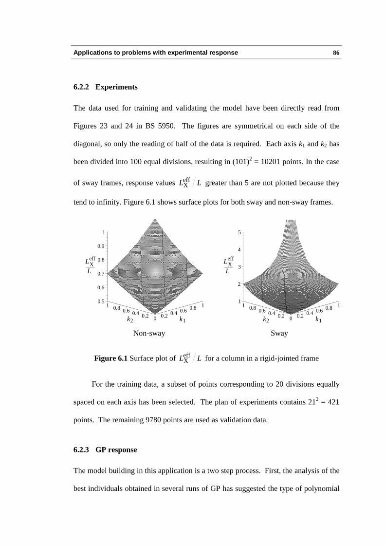
6.2.2 Experiments

The data used for training and validating the model have been directly read from

Figures 23 and 24 in BS 5950. The figures are symmetrical on each side of the

diagonal, so only the reading of half of the data is required. Each axis k1 and k2 has

been divided into 100 equal divisions, resulting in (101)2 = 10201 points. In the case

of sway frames, response values LLeffX greater than 5 are not plotted because they

tend to infinity. Figure 6.1 shows surface plots for both sway and non-sway frames.

0 0.2 0.4 0.6 0.8 1

k10.20.40.60.81

k2

0.5

0.6

0.7

0.8

0.9

1

LeffX

L

0 0.2 0.4 0.6 0.8 1

k10.20.40.60.81

k2

1

2

3

4

5

LeffX

L

Non-sway Sway

Figure 6.1 Surface plot of LLeffX for a column in a rigid-jointed frame

For the training data, a subset of points corresponding to 20 divisions equally

spaced on each axis has been selected. The plan of experiments contains 212 = 421

points. The remaining 9780 points are used as validation data.

6.2.3 GP response

The model building in this application is a two step process. First, the analysis of the

best individuals obtained in several runs of GP has suggested the type of polynomial


to be used. A typical expression in the case of columns in non-sway framework for

one run is as follows:

LLeffX = 0.5 + 0.14 k1 + 0.17 k2 + 0.092 k1

2 + 0.036 k22 -

0.12 k1 k2 + 0.34 k12 k2 + 0.17 k1 k2

2 - 0.031 k1

4 - 0.32 k13 k2

-

0.22 k12 k2

2 + 0.13 k13 k2

2 + 0.14 k14 k2

(6.1)

After careful comparison of the common terms of the best individuals in

several runs, a general structure for the expression has been assumed. The second

step has identified the tuning parameters that best fit the model into the training data.

A nonlinear optimization technique (Madsen and Hegelund, 1991) has been applied

to the following polynomial to find the coeff icients:

( ) ( ) ( ) ( ) ( )∑ ∑∑∑=

−

=

−

==

+++=m

i

i

j

jijij

m

i

ii

m

i

ii kkakakaakkF

2

1

1213

122

111021,

~(6.2)

where m is the order of the polynomial.

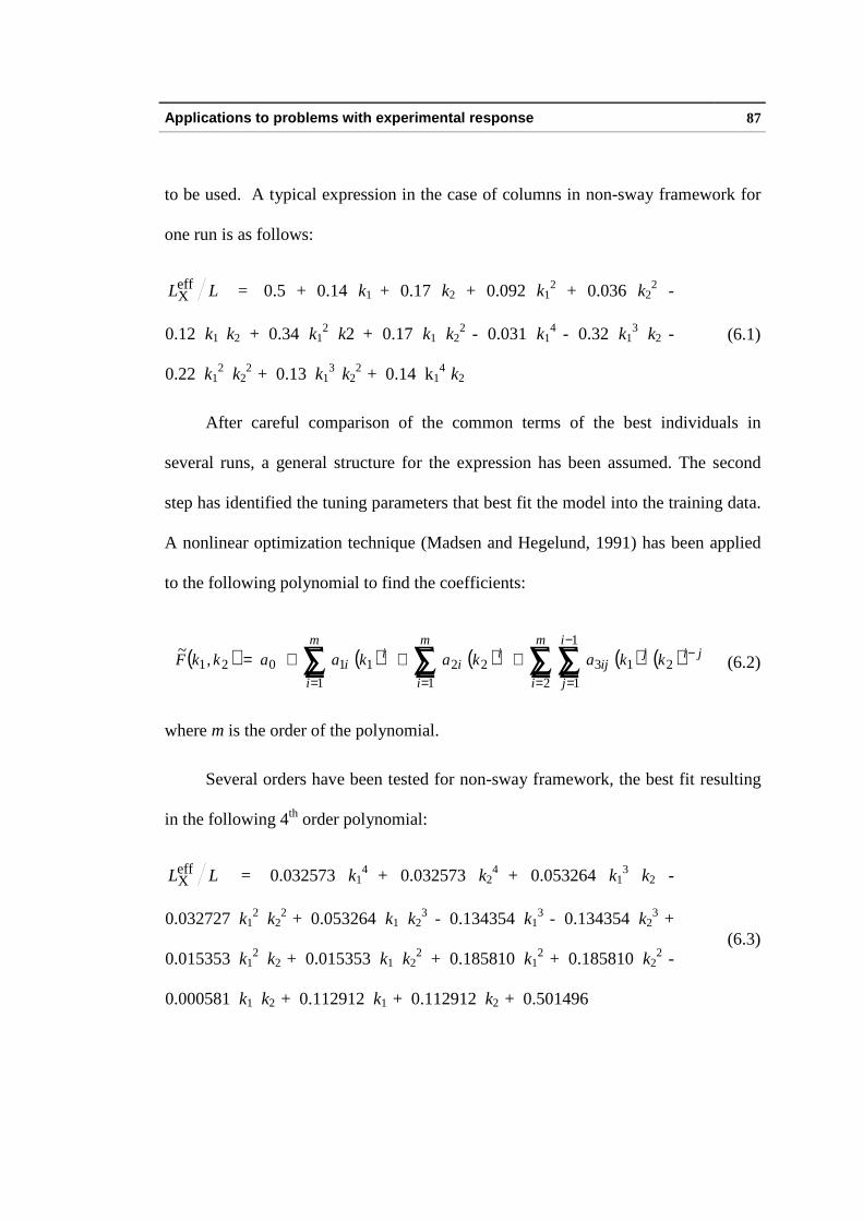
Several orders have been tested for non-sway framework, the best fit resulting

in the following 4th order polynomial:

LLeffX = 0.032573 k1

4 + 0.032573 k24 + 0.053264 k1

3 k2 -

0.032727 k12 k2

2 + 0.053264 k1 k23 - 0.134354 k1

3 - 0.134354 k23 +

0.015353 k12 k2 + 0.015353 k1 k2

2 + 0.185810 k12 + 0.185810 k2

2 -

0.000581 k1 k2 + 0.112912 k1 + 0.112912 k2 + 0.501496

(6.3)


The RMS error of expression (6.3) over the validation data is 0.011. This error

is acceptable taking into account the experimental error when reading the values

from the chart. Figure 6.2 represents the expression (6.3).

0 0.2 0.4 0.60.8 1

k 10.20.40.6

0.81

k2

0.5

0.6

0.7

0.8

0.9

1

LeffX

L

(a) Surface plot

1.0

0.5

0.75

0.55

0.85

0.575

0.625

0.95

0.675

0.6

0.8

0.65

0.7

0.525

0.9

0

0.1

0.2

0.3

0.4

0.5

0.6

0.7

0.8

0.9

1

k 2

0 0.1 0.2 0.3 0.4 0.5 0.6 0.7 0.8 0.9 1

k 1

(b) Contour plot

Figure 6.2 Graphical representation of the 4th order polynomial of LLeffX for a

column in a rigid-jointed non-sway frame


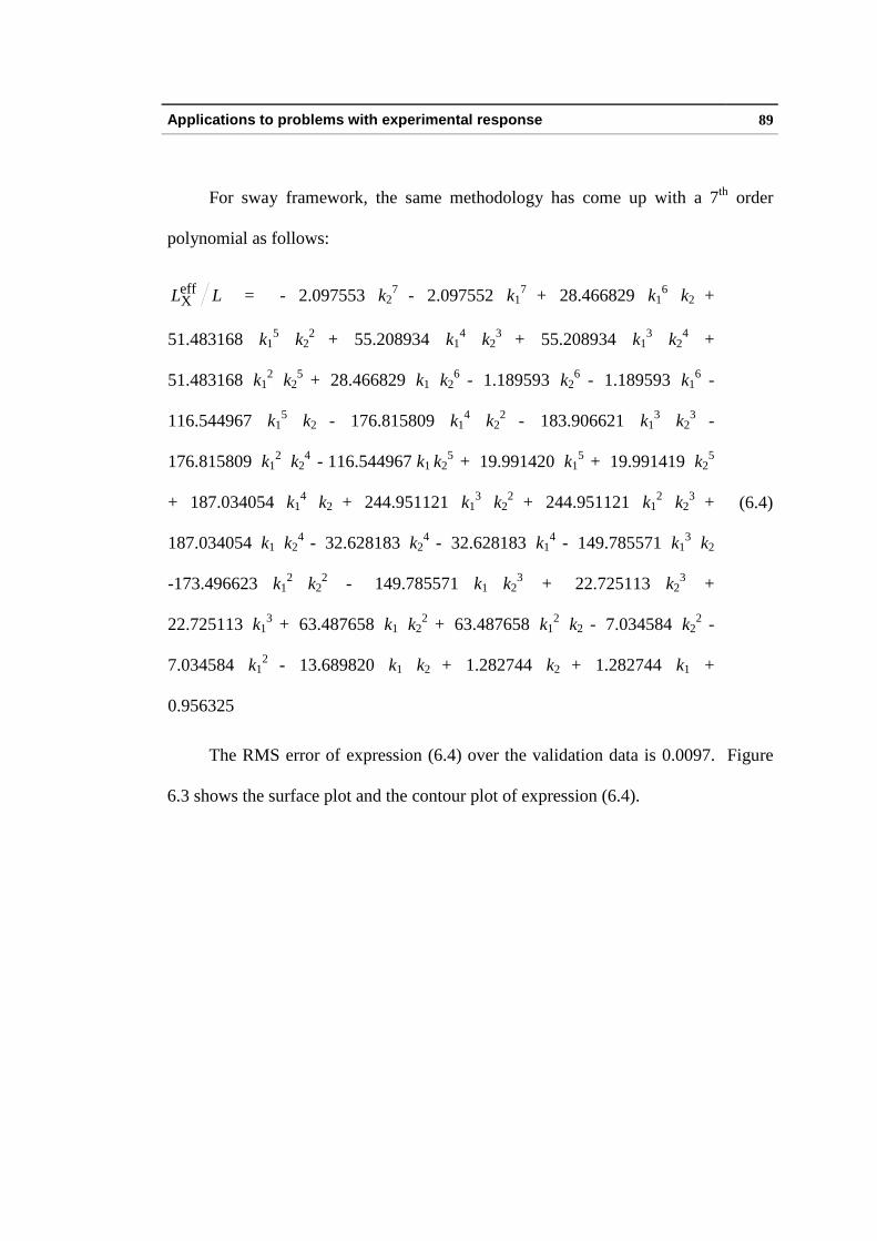
For sway framework, the same methodology has come up with a 7th order

polynomial as follows:

LLeffX = - 2.097553 k2

7 - 2.097552 k17 + 28.466829 k1

6 k2 +

51.483168 k15 k2

2 + 55.208934 k14 k2

3 + 55.208934 k13 k2

4 +

51.483168 k12 k2

5 + 28.466829 k1 k26 - 1.189593 k2

6 - 1.189593 k16 -

116.544967 k15 k2 - 176.815809 k1

4 k22 - 183.906621 k1

3 k23 -

176.815809 k12 k2

4 - 116.544967 k1 k25 + 19.991420 k1

5 + 19.991419 k25

+ 187.034054 k14 k2 + 244.951121 k1

3 k22 + 244.951121 k1

2 k23 +

187.034054 k1 k24 - 32.628183 k2

4 - 32.628183 k14 - 149.785571 k1

3 k2

-173.496623 k12 k2

2 - 149.785571 k1 k23 + 22.725113 k2

3 +

22.725113 k13 + 63.487658 k1 k2

2 + 63.487658 k12 k2 - 7.034584 k2

2 -

7.034584 k12 - 13.689820 k1 k2 + 1.282744 k2 + 1.282744 k1 +

0.956325

(6.4)

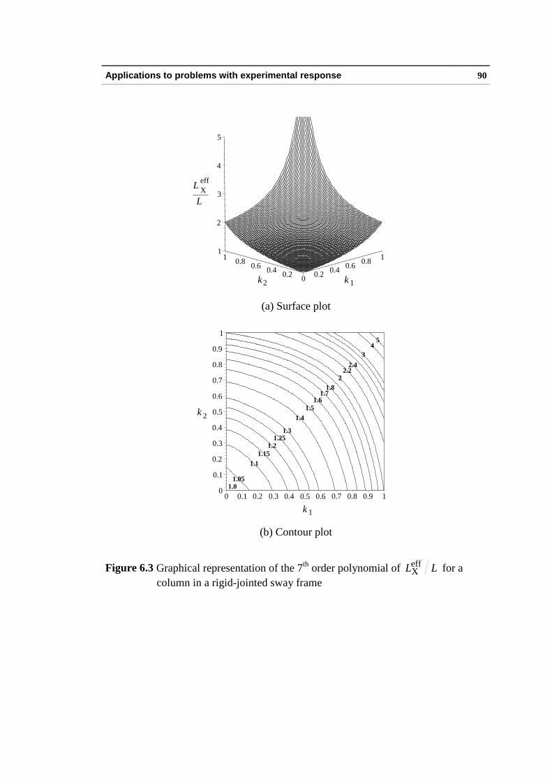
The RMS error of expression (6.4) over the validation data is 0.0097. Figure

6.3 shows the surface plot and the contour plot of expression (6.4).


0 0.2 0.4 0.60.8 1

k 10.20.40.6

0.81

k2

1

2

3

4

5

LeffX

L

(a) Surface plot

1.0

1.8

1.5 1.6

1.15

1.4

5

1.25

1.1

1.7

1.2

2.2

1.3

1.05

3

2

2.4

4

0

0.1

0.2

0.3

0.4

0.5

0.6

0.7

0.8

0.9

1

k 2

0 0.1 0.2 0.3 0.4 0.5 0.6 0.7 0.8 0.9 1

k 1

(b) Contour plot

Figure 6.3 Graphical representation of the 7th order polynomial of LLeffX for a

column in a rigid-jointed sway frame


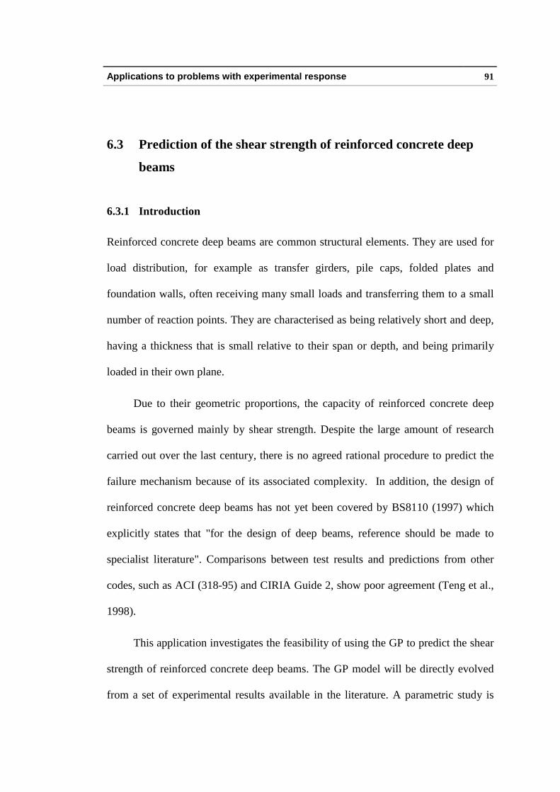
6.3 Prediction of the shear strength of reinforced concrete deep

beams

6.3.1 Introduction

Reinforced concrete deep beams are common structural elements. They are used for

load distribution, for example as transfer girders, pile caps, folded plates and

foundation walls, often receiving many small l oads and transferring them to a small

number of reaction points. They are characterised as being relatively short and deep,

having a thickness that is small relative to their span or depth, and being primarily

loaded in their own plane.

Due to their geometric proportions, the capacity of reinforced concrete deep

beams is governed mainly by shear strength. Despite the large amount of research

carried out over the last century, there is no agreed rational procedure to predict the

failure mechanism because of its associated complexity. In addition, the design of

reinforced concrete deep beams has not yet been covered by BS8110 (1997) which

explicitly states that "for the design of deep beams, reference should be made to

specialist literature". Comparisons between test results and predictions from other

codes, such as ACI (318-95) and CIRIA Guide 2, show poor agreement (Teng et al.,

1998).

This application investigates the feasibili ty of using the GP to predict the shear

strength of reinforced concrete deep beams. The GP model will be directly evolved

from a set of experimental results available in the literature. A parametric study is


conducted to examine the validity of the GP model predictions outside the range

defined for its construction.

6.3.2 Training data

The main parameters influencing the shear strength of reinforced concrete deep

beams are the concrete compressive strength, main longitudinal bottom

reinforcement, horizontal and vertical web reinforcement, beam width and depth,

shear-span and beam-span (Ashour, 2000, Kong et al., 1970, Smith and Vantsiotis,

1982).

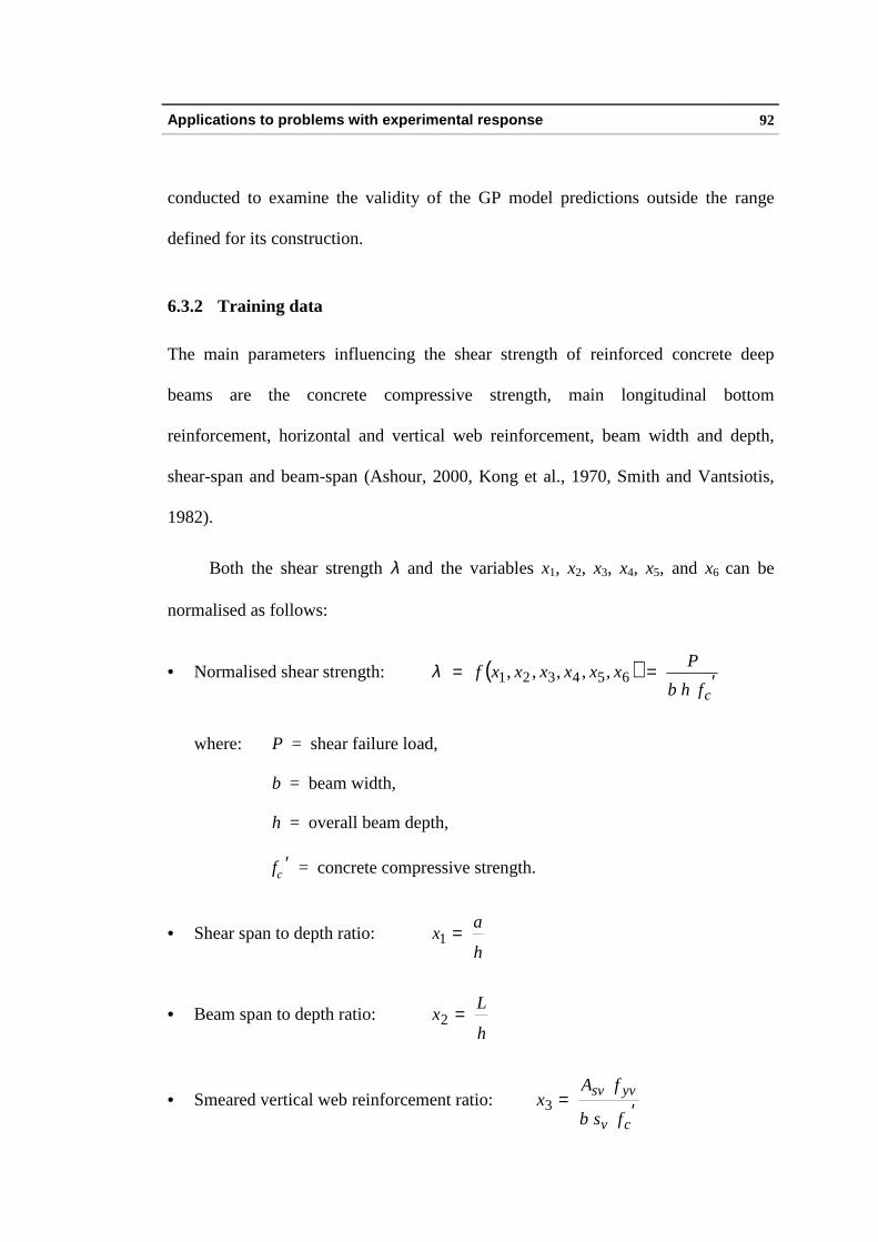
Both the shear strength λ and the variables x1, x2, x3, x4, x5, and x6 can be

normalised as follows:

• Normalised shear strength: ( ) ′==cfhb

Pxxxxxxf 654321 ,,,,,λ

where: P = shear failure load,

b = beam width,

h = overall beam depth,

fc ′ = concrete compressive strength.

• Shear span to depth ratio: h

ax =1

• Beam span to depth ratio: h

Lx =2

• Smeared vertical web reinforcement ratio: ′=cv

yvsv

fsb

fAx3


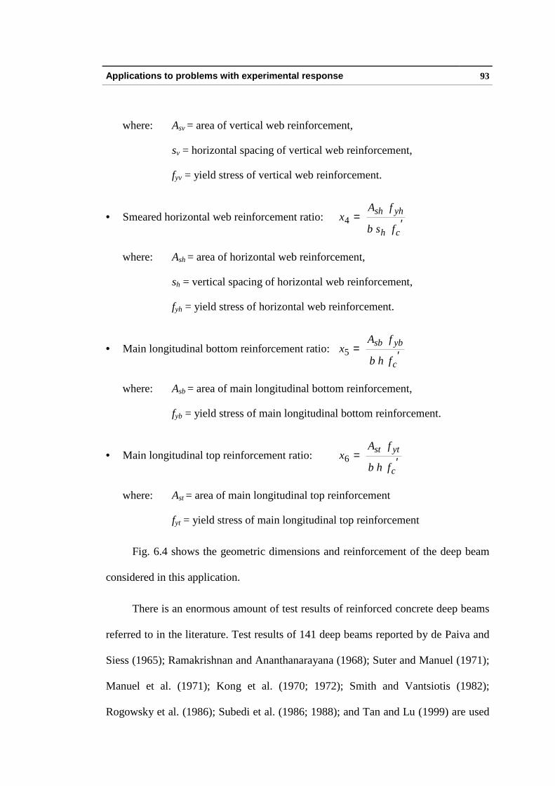
where: Asv = area of vertical web reinforcement,

sv = horizontal spacing of vertical web reinforcement,

fyv = yield stress of vertical web reinforcement.

• Smeared horizontal web reinforcement ratio: ′=ch

yhsh

fsb

fAx4

where: Ash = area of horizontal web reinforcement,

sh = vertical spacing of horizontal web reinforcement,

fyh = yield stress of horizontal web reinforcement.

• Main longitudinal bottom reinforcement ratio: ′=c

ybsb

fhb

fAx5

where: Asb = area of main longitudinal bottom reinforcement,

fyb = yield stress of main longitudinal bottom reinforcement.

• Main longitudinal top reinforcement ratio: ′=c

ytst

fhb

fAx6

where: Ast = area of main longitudinal top reinforcement

fyt = yield stress of main longitudinal top reinforcement

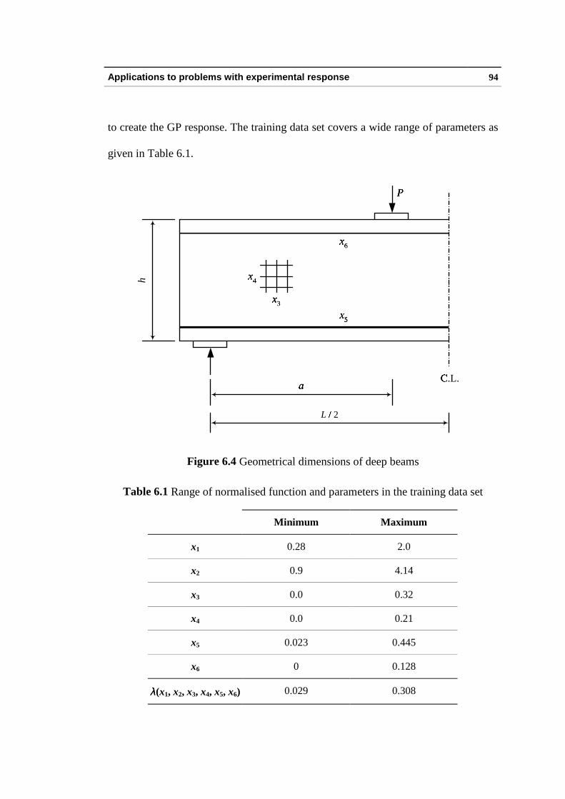
Fig. 6.4 shows the geometric dimensions and reinforcement of the deep beam

considered in this application.

There is an enormous amount of test results of reinforced concrete deep beams

referred to in the literature. Test results of 141 deep beams reported by de Paiva and

Siess (1965); Ramakrishnan and Ananthanarayana (1968); Suter and Manuel (1971);

Manuel et al. (1971); Kong et al. (1970; 1972); Smith and Vantsiotis (1982);

Rogowsky et al. (1986); Subedi et al. (1986; 1988); and Tan and Lu (1999) are used


to create the GP response. The training data set covers a wide range of parameters as

given in Table 6.1.

L / � 2

h

x �3

�

x �4

�

x �6

�

x �5

�

a � C.L. �

P �

Figure 6.4 Geometrical dimensions of deep beams

Table 6.1 Range of normalised function and parameters in the training data set

Minimum Maximum

x1 0.28 2.0

x2 0.9 4.14

x3 0.0 0.32

x4 0.0 0.21

x5 0.023 0.445

x6 0 0.128

λλ(x1, x2, x3, x4, x5, x6) 0.029 0.308


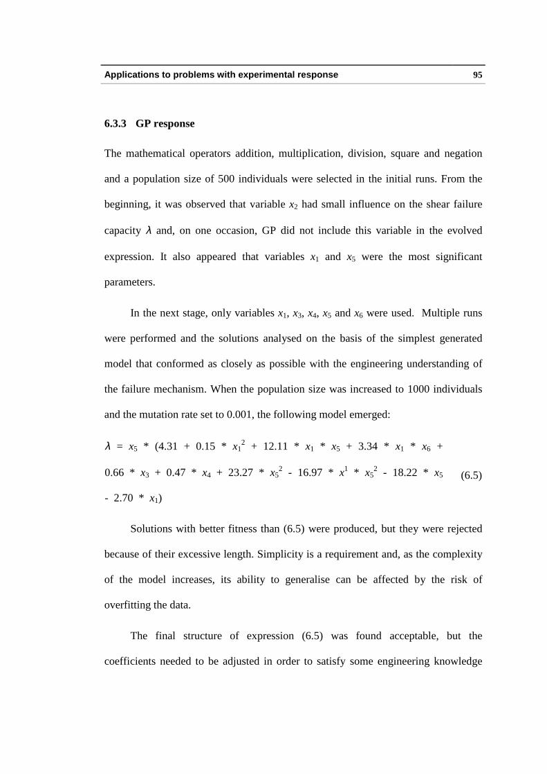
6.3.3 GP response

The mathematical operators addition, multiplication, division, square and negation

and a population size of 500 individuals were selected in the initial runs. From the

beginning, it was observed that variable x2 had small i nfluence on the shear failure

capacity λ and, on one occasion, GP did not include this variable in the evolved

expression. It also appeared that variables x1 and x5 were the most significant

parameters.

In the next stage, only variables x1, x3, x4, x5 and x6 were used. Multiple runs

were performed and the solutions analysed on the basis of the simplest generated

model that conformed as closely as possible with the engineering understanding of

the failure mechanism. When the population size was increased to 1000 individuals

and the mutation rate set to 0.001, the following model emerged:

λ = x5 * (4.31 + 0.15 * x12 + 12.11 * x1 * x5 + 3.34 * x1 * x6 +

0.66 * x3 + 0.47 * x4 + 23.27 * x52 - 16.97 * x1 * x5

2 - 18.22 * x5

- 2.70 * x1)

(6.5)

Solutions with better fitness than (6.5) were produced, but they were rejected

because of their excessive length. Simplicity is a requirement and, as the complexity

of the model increases, its abili ty to generalise can be affected by the risk of

overfitting the data.

The final structure of expression (6.5) was found acceptable, but the

coeff icients needed to be adjusted in order to satisfy some engineering knowledge


constraints (λ > 0). A sequential quadratic programming (SQP) algorithm (Madsen

and Tingleff , 1990) was applied to produce the final model, as follows:

λ = x5 * (3.50 + 0.20 * x12 - 1.76 * x1 + x1 * (3.3 * x5 +

3.37 * x6 - 1.66 * x52) - 10.67 * x5 + 9.8 * x5

2 + 0.63 * x3 +

0.71 * x4)

(6.6)

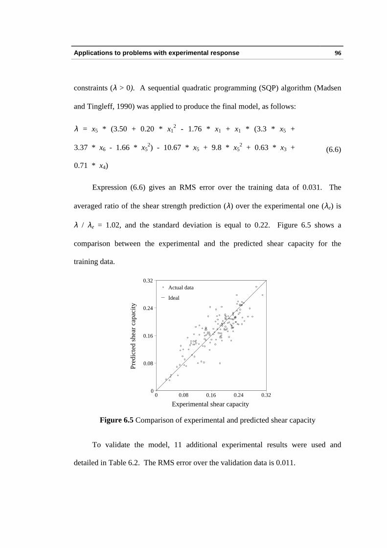
Expression (6.6) gives an RMS error over the training data of 0.031. The

averaged ratio of the shear strength prediction (λ) over the experimental one (λe) is

λ / λe = 1.02, and the standard deviation is equal to 0.22. Figure 6.5 shows a

comparison between the experimental and the predicted shear capacity for the

training data.

Actual data

Ideal

0

0.08

0.16

0.24

0.32

0 0.08 0.16 0.24 0.32

Experimental shear capacity

Pre

dict

ed s

hear

cap

acity

Figure 6.5 Comparison of experimental and predicted shear capacity

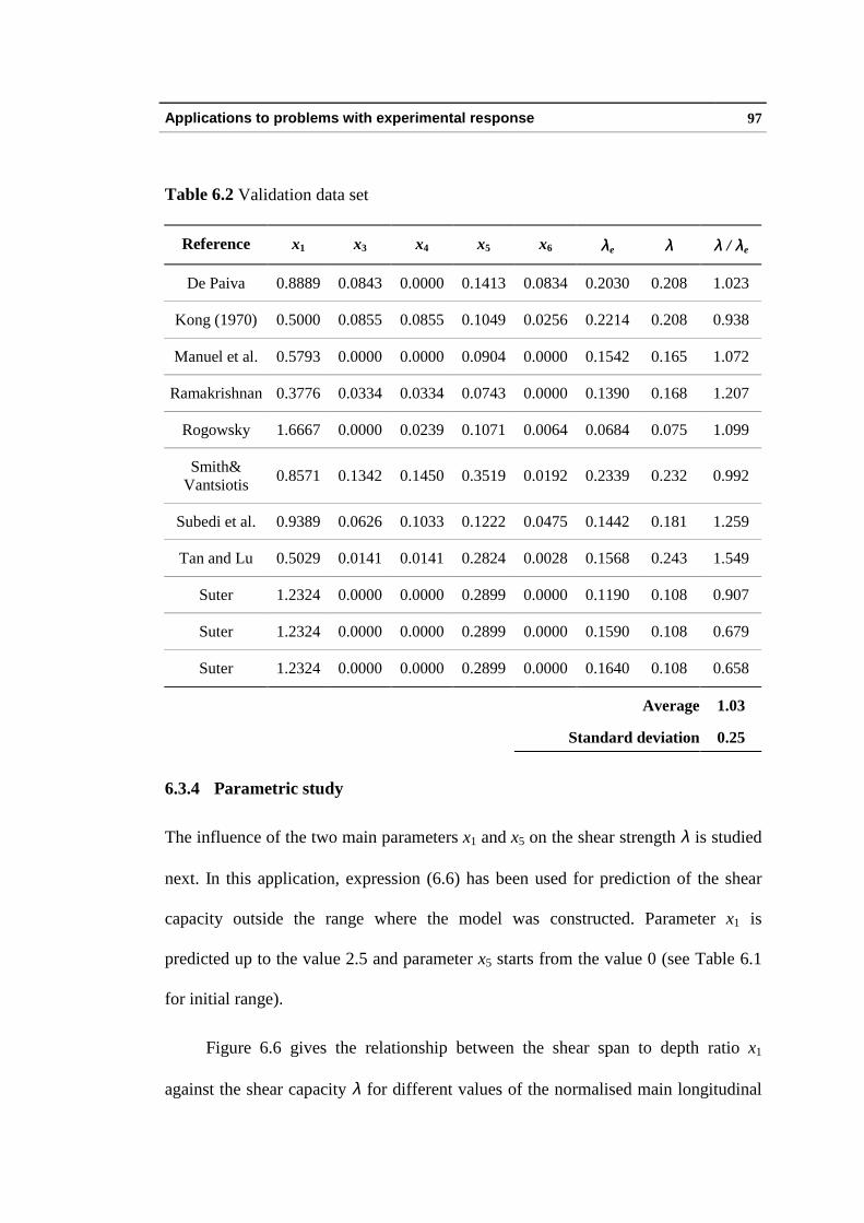
To validate the model, 11 additional experimental results were used and

detailed in Table 6.2. The RMS error over the validation data is 0.011.


Table 6.2 Validation data set

Reference x1 x3 x4 x5 x6 λλe λλ λλ / λλe

De Paiva 0.8889 0.0843 0.0000 0.1413 0.0834 0.2030 0.208 1.023

Kong (1970) 0.5000 0.0855 0.0855 0.1049 0.0256 0.2214 0.208 0.938

Manuel et al. 0.5793 0.0000 0.0000 0.0904 0.0000 0.1542 0.165 1.072

Ramakrishnan 0.3776 0.0334 0.0334 0.0743 0.0000 0.1390 0.168 1.207

Rogowsky 1.6667 0.0000 0.0239 0.1071 0.0064 0.0684 0.075 1.099

Smith&Vantsiotis

0.8571 0.1342 0.1450 0.3519 0.0192 0.2339 0.232 0.992

Subedi et al. 0.9389 0.0626 0.1033 0.1222 0.0475 0.1442 0.181 1.259

Tan and Lu 0.5029 0.0141 0.0141 0.2824 0.0028 0.1568 0.243 1.549

Suter 1.2324 0.0000 0.0000 0.2899 0.0000 0.1190 0.108 0.907

Suter 1.2324 0.0000 0.0000 0.2899 0.0000 0.1590 0.108 0.679

Suter 1.2324 0.0000 0.0000 0.2899 0.0000 0.1640 0.108 0.658

Average 1.03

Standard deviation 0.25

6.3.4 Parametric study

The influence of the two main parameters x1 and x5 on the shear strength λ is studied

next. In this application, expression (6.6) has been used for prediction of the shear

capacity outside the range where the model was constructed. Parameter x1 is

predicted up to the value 2.5 and parameter x5 starts from the value 0 (see Table 6.1

for initial range).

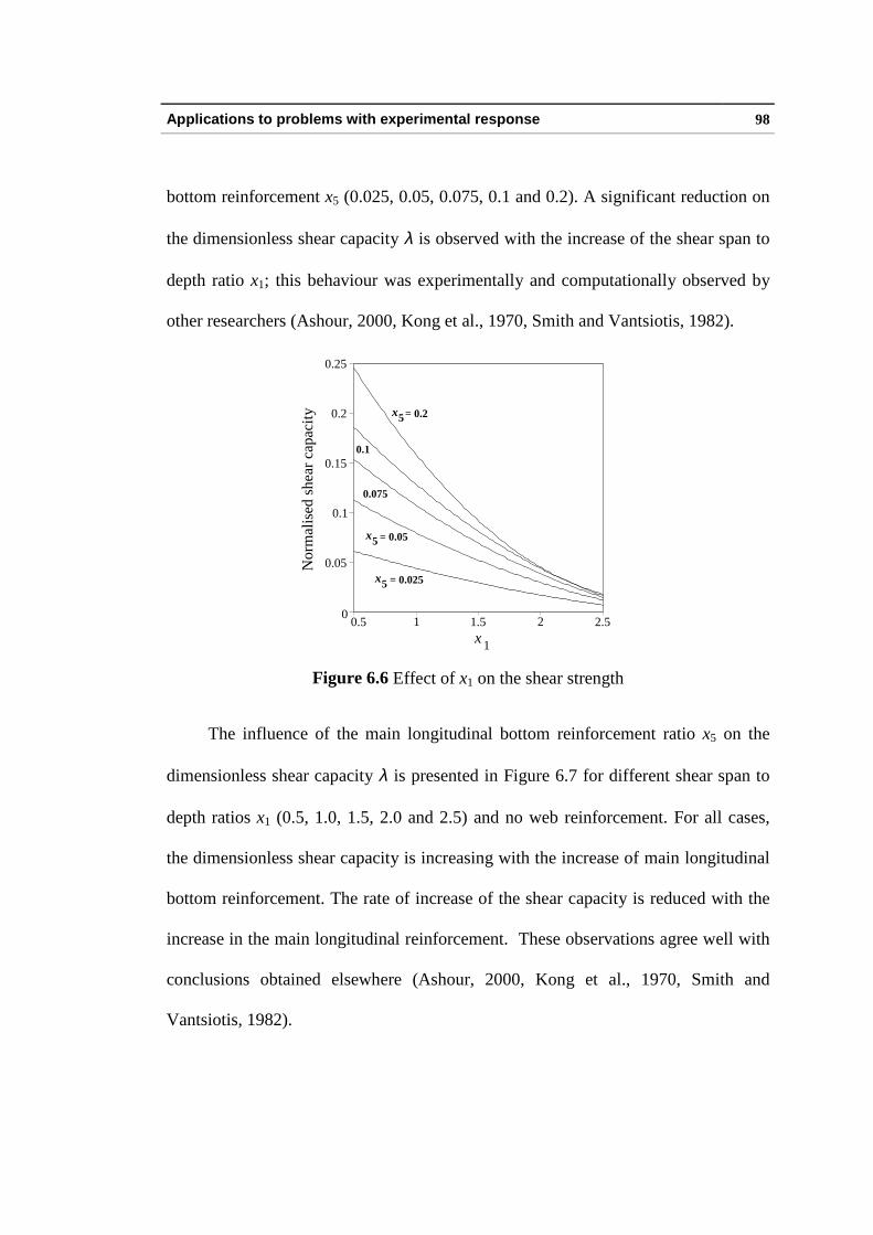
Figure 6.6 gives the relationship between the shear span to depth ratio x1

against the shear capacity λ for different values of the normalised main longitudinal


bottom reinforcement x5 (0.025, 0.05, 0.075, 0.1 and 0.2). A significant reduction on

the dimensionless shear capacity λ is observed with the increase of the shear span to

depth ratio x1; this behaviour was experimentally and computationally observed by

other researchers (Ashour, 2000, Kong et al., 1970, Smith and Vantsiotis, 1982).

= 0.0255

= 0.055

0.075

0.1

= 0.25

x

x

x

0

0.05

0.1

0.15

0.2

0.25

0.5 1 1.5 2 2.5x 1

Nor

mal

ised

she

ar c

apac

ity

Figure 6.6 Effect of x1 on the shear strength

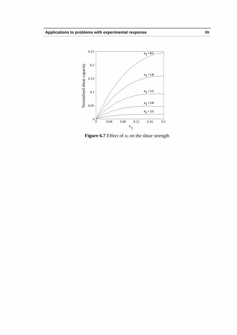
The influence of the main longitudinal bottom reinforcement ratio x5 on the

dimensionless shear capacity λ is presented in Figure 6.7 for different shear span to

depth ratios x1 (0.5, 1.0, 1.5, 2.0 and 2.5) and no web reinforcement. For all cases,

the dimensionless shear capacity is increasing with the increase of main longitudinal

bottom reinforcement. The rate of increase of the shear capacity is reduced with the

increase in the main longitudinal reinforcement. These observations agree well with

conclusions obtained elsewhere (Ashour, 2000, Kong et al., 1970, Smith and

Vantsiotis, 1982).


= 2.51

= 2.01

= 1.51

= 1.01

= 0.51

x

x

x

x

x

0

0.05

0.1

0.15

0.2

0.25

0 0.04 0.08 0.12 0.16 0.2x5

Nor

mal

ised

she

ar c

apac

ity

Figure 6.7 Effect of x5 on the shear strength


6.4 Multicriteria optimization of the calcination of Roman cement

6.4.1 Introduction

In the 19th century, Roman cement was used throughout Europe for the production of

stucco finishes in architectural decoration. However, problems with the supply of

raw materials and developments in Portland cements motivated the decline in its use

and the corresponding loss of craft techniques.

The Charter of Venice (1964) states that the process of restoration should be

based on respect for the original material. This is in contrast with the use of the

current modern cement products, finishing layers and paints that do not match the

original physical and mechanical properties of the stuccoes.

Consequently, for the re-introduction of Roman cement, there is a need to find

a suitable range of similar materials among the re-emerging natural hydraulic

binders, and to appreciate the technical knowledge and understanding of the original

cement-makers. Hughes et al. (1999) have reported experimental results on the

calcination of cement-stones from the Harwich and Whitby group of cements. This

shows that both setting time and strength development are functions of source and

calcination temperature.

In this application, a single source of cement-stone was identified for

experimentation within an optimization programme to relate mechanical and

mineralogical characteristics to calcination conditions. Genetic programming has

been used to ill ustrate the general trends of minerals and the strength development of


the cement. The data will be useful for the selection of hydraulic binders and as an

element in the re-introduction of Roman cement to the European market.

6.4.2 Experimental work

The cement-stones used in this research were collected from the Yorkshire coast at

Whitby Long Bight.

The calcination process is not well documented in the historic literature.

Previous work at Bradford University has utili sed temperatures of 940°C and 1100°C

and found the lower temperature to offer better product (Hughes et al., 1999). For

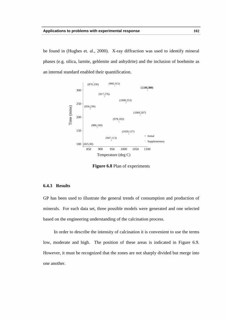
the current research, the Audze-Eglais plan of experiments shown in Figure 6.8 has

been used with 10 initial and 2 supplementary points. Each cement is referred to

using the nomenclature of temperature and residence time, e.g. 917/276 taken as

design variables x1 and x2 respectively. An electric kiln was used and no attempt

made to either circulate air through it or to seal it during calcination. It is therefore

to be expected that some cements would be produced under reducing conditions (low

oxygen content in the kiln). As more experience is gained of this group of cements,

this and additional factors will be added to future optimization programmes.

Ten kilogram batches of raw material underwent an overnight pre-soak at

300°C prior to increasing the temperature. This procedure was introduced in earlier

programmes to prevent the explosive disintegration of larger stone fragments in the

kiln. The kiln was raised to the required temperature maintained for the specified

time and then allowed to cool overnight before the samples were removed for

grinding. All cements were ground to <150µm. Characteristics of the cements may


be found in (Hughes et. al., 2000). X-ray diffraction was used to identify mineral

phases (e.g. sili ca, larnite, gehlenite and anhydrite) and the inclusion of boehmite as

an internal standard enabled their quantification.

Supplementary

Initial

(870,330)(1100,300)(1100,300)

(960,315)

(1069,207)

(1020,137)

(1008,253)

(978,183)

(947,113)

(917,276)

(886,160)

(856,230)

(825,90)100

150

200

250

300

850 900 950 1000 1050 1100

Temperature (deg C)

Tim

e (m

ins)

Figure 6.8 Plan of experiments

6.4.3 Results

GP has been used to ill ustrate the general trends of consumption and production of

minerals. For each data set, three possible models were generated and one selected

based on the engineering understanding of the calcination process.

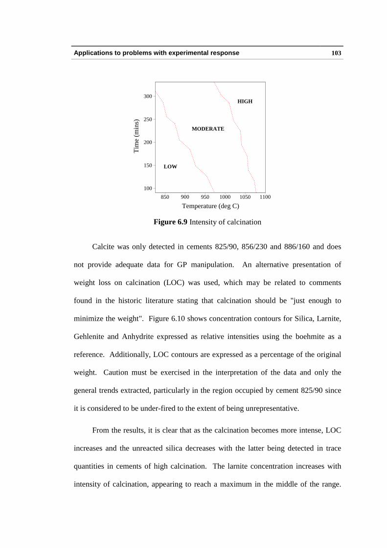
In order to describe the intensity of calcination it is convenient to use the terms

low, moderate and high. The position of these areas is indicated in Figure 6.9.

However, it must be recognized that the zones are not sharply divided but merge into

one another.


HIGH

MODERATE

LOW

100

150

200

250

300

850 900 950 1000 1050 1100

Temperature (deg C)

Tim

e (m

ins)

Figure 6.9 Intensity of calcination

Calcite was only detected in cements 825/90, 856/230 and 886/160 and does

not provide adequate data for GP manipulation. An alternative presentation of

weight loss on calcination (LOC) was used, which may be related to comments

found in the historic literature stating that calcination should be "just enough to

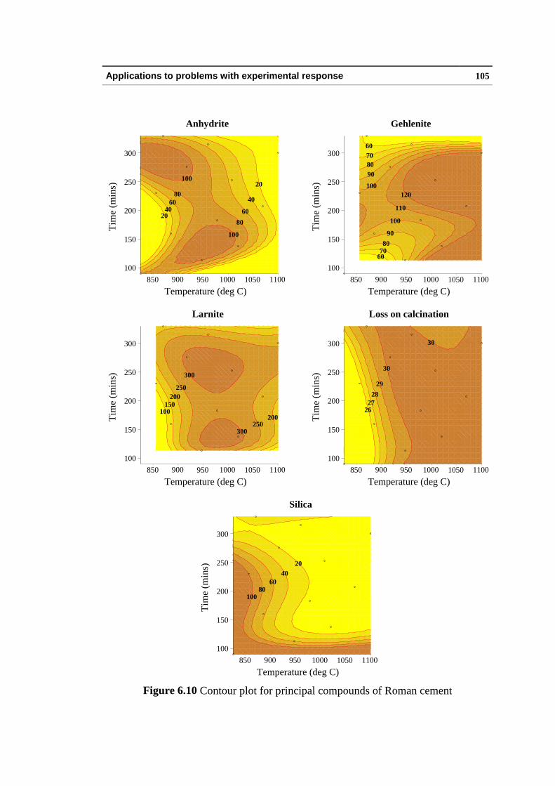
minimize the weight". Figure 6.10 shows concentration contours for Sili ca, Larnite,

Gehlenite and Anhydrite expressed as relative intensities using the boehmite as a

reference. Additionally, LOC contours are expressed as a percentage of the original

weight. Caution must be exercised in the interpretation of the data and only the

general trends extracted, particularly in the region occupied by cement 825/90 since

it is considered to be under-fired to the extent of being unrepresentative.

From the results, it is clear that as the calcination becomes more intense, LOC

increases and the unreacted sili ca decreases with the latter being detected in trace

quantities in cements of high calcination. The larnite concentration increases with

intensity of calcination, appearing to reach a maximum in the middle of the range.


Whilst gehlenite is always present, its maximum is at a higher intensity of calcination

than noted for larnite. Any link between the decrease in larnite and increase in

gehlenite must await further investigation.

Figure 6.10 also shows the concentration of anhydrite to be calcination

dependent. The decline in anhydrite with more intense calcinations was

accompanied by the emergence of Ye'elminite. Cements 825/90, 856/230, 886/160

and 947/113 also show the presence of calcium sulfite, which is associated with

reducing conditions. Pastes of these cements turned green when immersed in water,

albeit very slight in the case of 947/113 which also only contained a trace of the

sulfite.

All cements registered a final setting time much shorter than that of Portland

cement, with values in the range 30 seconds to 113 minutes.

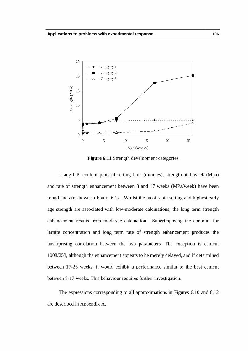
Strength development has been determined up to an age of 6 months and 3

broad categories of development identified, which correspond to the 3 intensities of

calcination decribed in Figure 6.11. Category 1 is associated with low intensity

calcination conditions, category 2 follows moderate calcination and category 3 is

displayed following high calcination.

Historically, Roman cements were often compared for quali ty on the basis of

the rapidity of their set, although it should be recognised that the rapid setting times

of some of the current pastes are shorter than those prevalent in the 19th century

(typically 5-15 minutes).


2060

80

406080

100

40

20

100

100

150

200

250

300

850 900 950 1000 1050 1100

Temperature (deg C)

AnhydriteT

ime

(min

s)

100

100

90

60

80

90

70

8070

110

120

60

100

150

200

250

300

850 900 950 1000 1050 1100

Temperature (deg C)

Gehlenite

Tim

e (m

ins)

300

300

250200

250

100150

200

100

150

200

250

300

850 900 950 1000 1050 1100

Temperature (deg C)

Larnite

Tim

e (m

ins)

30

29

2726

28

30

100

150

200

250

300

850 900 950 1000 1050 1100

Temperature (deg C)

Loss on calcinationT

ime

(min

s)

100

4020

6080

100

150

200

250

300

850 900 950 1000 1050 1100

Temperature (deg C)

Silica

Tim

e (m

ins)

Figure 6.10 Contour plot for principal compounds of Roman cement


0

5

10

15

20

25

0 5 10 15 20 25

Age (weeks)

Str

en

gth

(M

Pa

)Category 1

Category 2

Category 3

Figure 6.11 Strength development categories

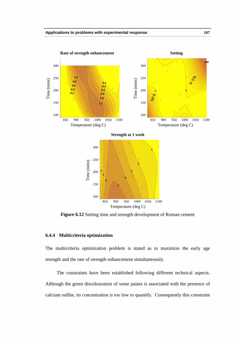
Using GP, contour plots of setting time (minutes), strength at 1 week (Mpa)

and rate of strength enhancement between 8 and 17 weeks (MPa/week) have been

found and are shown in Figure 6.12. Whilst the most rapid setting and highest early

age strength are associated with low-moderate calcinations, the long term strength

enhancement results from moderate calcination. Superimposing the contours for

larnite concentration and long term rate of strength enhancement produces the

unsurprising correlation between the two parameters. The exception is cement

1008/253, although the enhancement appears to be merely delayed, and if determined

between 17-26 weeks, it would exhibit a performance similar to the best cement

between 8-17 weeks. This behaviour requires further investigation.

The expressions corresponding to all approximations in Figures 6.10 and 6.12

are described in Appendix A.


0.20.6

0.8

1.0

1.0

0.20.4

1.2

0.4

0.8

0.6

100

150

200

250

300

850 900 950 1000 1050 1100

Temperature (deg C)

Rate of strength enhancementT

ime

(min

s)

100

5 5

2015

10

10

1520

100

150

200

250

300

850 900 950 1000 1050 1100

Temperature (deg C)

Setting

Tim

e (m

ins)

2

32

44

5

1

3

100

150

200

250

300

850 900 950 1000 1050 1100

Temperature (deg C)

Strength at 1 week

Tim

e (m

ins)

Figure 6.12 Setting time and strength development of Roman cement

6.4.4 Multicriteria optimization

The multicriteria optimization problem is stated as to maximize the early age

strength and the rate of strength enhancement simultaneously.

The constraints have been established following different technical aspects.

Although the green discolouration of some pastes is associated with the presence of

calcium sulfite, its concentration is too low to quantify. Consequently this constraint


has been represented by a maximum sili ca content (determined by X-ray difraction

using boehmite as an internal standard) expressed as relative intensity 50. This

correlates with pastes which do not turn green. Further work on the materials aspect

of the investigation is required to refine this constraint and provide a direct measure

of greenness. The LOC of 28-30% has been selected to represent the confused

historic statements of "calcine suff icient to decarbonate", "just enough to minimize

the weight" and "underfire to economize on grounding" found in the literature.

The setting time constraint imposes an artificially tight limitation since

historical Roman cements which set too rapidly were exposed to the air for a short

period of time. A thin layer of cement 917/276 was exposed to the laboratory air for

24 hours and subsequently assessed for setting and strength development. The

setting time was increased from 30 seconds to 5 minutes. The early age strength and

the rate of strength enhancement was slightly decreased, but still yielded an excellent

product.

Knowing that the setting could be controlled naturally, this constraint was

removed and the multicriteria optimization problem defined. Table 6.3 shows the

formulation of the optimization problem.

Table 6.3 Definition of the optimization problems

Strength at 1 week

Rate of strength enhancement

→ max

→ max

Subject to:Sili ca ≤ 50

28% ≤ LOC ≤ 30%


6.4.5 Pareto-optimal solution set

A characteristic of problems with multiple criteria is that the solutions in the search

space are not optimal from the point of view of any single objective, therefore the

objective functions are in conflict with one another. A set of solutions must be found

such that it is not possible to improve any of them without deteriorating at least one

of the other objective functions. These solutions are known as Pareto-optimal

solutions. Solutions belonging to the Pareto-optimal set are to be considered by a

specialist and a single solution can then be established on the basis of some

additional information, e.g. about the relative merits of these criteria or some

additional criteria. The choice of one particular solution is a compromise decision

that depends on the features of the particular problem and the knowledge of the

designer concerning the problem.

A vector x* is Pareto-optimal i f and only if there is no vector x such that

Fj (x) ≥ Fj (x*) for all j = 1,...,m

Fj (x) > Fj (x*) for at least one j = 1,...,m

(6.7)

For all non-Pareto-optimal vectors, the value of at least one objective function

Fj can be increased without decreasing the functional values of the other

components.

To find the Pareto-optimal set, first the objective and constraint functions have

been plotted to identify the feasible solution domain. Second, the numerical solution

has been performed by an SQP algorithm (Madsen and Tingleff , 1990) at regular

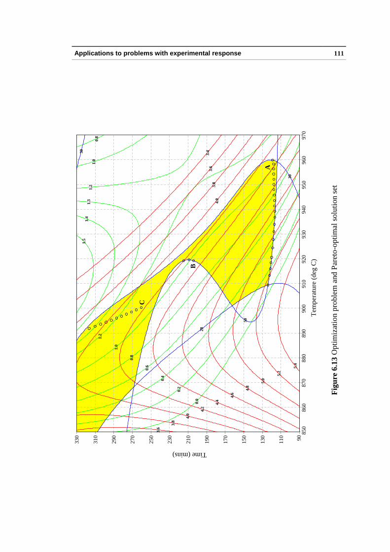
intervals. The final solution is represented in Figure 6.13. The yellow areas define


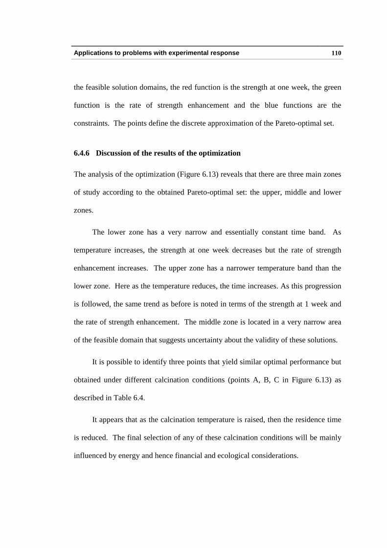
the feasible solution domains, the red function is the strength at one week, the green

function is the rate of strength enhancement and the blue functions are the

constraints. The points define the discrete approximation of the Pareto-optimal set.

6.4.6 Discussion of the results of the optimization

The analysis of the optimization (Figure 6.13) reveals that there are three main zones

of study according to the obtained Pareto-optimal set: the upper, middle and lower

zones.

The lower zone has a very narrow and essentially constant time band. As

temperature increases, the strength at one week decreases but the rate of strength

enhancement increases. The upper zone has a narrower temperature band than the

lower zone. Here as the temperature reduces, the time increases. As this progression

is followed, the same trend as before is noted in terms of the strength at 1 week and

the rate of strength enhancement. The middle zone is located in a very narrow area

of the feasible domain that suggests uncertainty about the validity of these solutions.

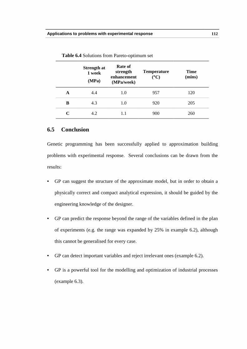
It is possible to identify three points that yield similar optimal performance but

obtained under different calcination conditions (points A, B, C in Figure 6.13) as

described in Table 6.4.

It appears that as the calcination temperature is raised, then the residence time

is reduced. The final selection of any of these calcination conditions will be mainly

influenced by energy and hence financial and ecological considerations.


A

B

C

1.0

0.8

1.4

0.8

1.2

0.6

1.2

0.4

0.0

1.3

1.5

0.2

1.0

3.8

5.2

4.0

3.4

4.0

3.6

4.8

4.2

3.6

5.0

4.6

3.8

4.4

5.4

30

30

28

50

90110

130

150

170

190

210

230

250

270

290

310

330 85

086

087

088

089

090

091

092

093

094

095

096

097

0

Tem

pera

ture

(de

g C

)

Time (mins)

Fig

ure

6.13

Opt

imiz

atio

n pr

oble

m a

nd P

aret

o-op

timal

sol

utio

n se

t


Table 6.4 Solutions from Pareto-optimum set

Strength at1 week

(MPa)

Rate ofstrength

enhancement(MPa/week)

Temperature(°°C)

Time(mins)

A 4.4 1.0 957 120

B 4.3 1.0 920 205

C 4.2 1.1 900 260

6.5 Conclusion

Genetic programming has been successfully applied to approximation building

problems with experimental response. Several conclusions can be drawn from the

results:

• GP can suggest the structure of the approximate model, but in order to obtain a

physically correct and compact analytical expression, it should be guided by the

engineering knowledge of the designer.

• GP can predict the response beyond the range of the variables defined in the plan

of experiments (e.g. the range was expanded by 25% in example 6.2), although

this cannot be generalised for every case.

• GP can detect important variables and reject irrelevant ones (example 6.2).

• GP is a powerful tool for the modelli ng and optimization of industrial processes

(example 6.3).

Documents

Applications to problems with experimental response · Applications to problems with experimental response 85 ... and CIRIA Guide 2, show poor agreement (Teng et ... Applications