APPLICATIONS OF SOLIDWORKS FLOW SIMULATION … · applications of solidworks flow simulation computational fluid dynamics software to the investigation of fires by: john b. holecek,

APPLICATIONS OF SOLIDWORKS FLOW SIMULATION COMPUTATIONAL FLUID DYNAMICS SOFTWARE TO THE INVESTIGATION OF FIRES

John B. Holecek, P.E., CFEI, Senior Consulting Engineer, Warren _____________________________________________________________

Abstract

NFPA 921 advises the use of a systematic approach to fire investigation that is best embodied by the scientific method. The scientific method includes the steps of collecting data, analyzing that data, developing a hypothesis, and then testing that hypothesis. The final step of this process, testing the hypothesis, can be done either physically or analytically. In some cases, a physical test may be conducted to confirm or falsify some aspect of the hypothesis. However, in many cases creating a physical test may be difficult or even practically impossible. It is these cases, and others, where analytic testing using computer simulations may be helpful to the fire investigator. The use of computer simulations in fire investigation is not a new concept. Computer models have been used to model fire behavior since at least the mid 1970’s. Today, software such as NIST supported Fire Dynamics Simulator is used with some frequency for analytic testing of fire origin and cause hypotheses. Third party software, such as PyroSim have been developed that eases the user interaction with the core FDS code. In parallel with the development of computer modeling tools specific to fire investigation or fire engineering, many developments have occurred in the much larger world of 3D computer aided design and engineering tools (CAD/CAE). SOLIDWORKS is a widely used suite of 3D CAD/CAE products typically used in the design of products. The software is separated into various modules that seamlessly integrate. The software starts with a CAD package that allows the creation and management of three-dimensional geometries. Mechanical simulation packages that allow many forms of stress and mechanical analysis are available. More applicable to fire investigation, SOLIDWORKS has a Flow Simulation package that utilizes Computational Fluid Dynamics (CFD) for the analysis of fluid flow and heat transfer.

APPLICATIONS OF SOLIDWORKS FLOW SIMULATION COMPUTATIONAL FLUID DYNAMICS SOFTWARE TO THE INVESTIGATION OF FIRES By: John B. Holecek, P.E., CFEI

Page 2

The author has experience in the use of SOLIDWORKS’ suite of product design software and has applied their Flow Simulation software to the solution of several problems related to fire investigation. For example, one application relates to testing the potential of a heat producing device to be a competent ignition source in a hypothesized ignition sequence. In this paper, two simulations with applications to fire investigation are examined and modeled using SOLIDWORKS Flow Simulation software. The results of the modeling are presented, along with data from real physical testing that seek to validate the SOLIDWORKS Flow Simulation model. Also presented are some limitations of Flow Simulation software as applied to fire investigation. Consulting the information presented should assist the investigator in correctly applying SOLIDWORKS, or other commercial product design software incorporating CFD, to certain aspects of fire investigation analytic testing. Introduction

Computational Fluid Dynamics (CFD) is a branch of applied science that utilizes computer numerical methods to solve problems of fluid flows and heat transfer. These problems are generally complex such that closed form solutions are not available. CFD generally involves three overall steps, pre-processing, simulation, and post processing. These steps may be accomplished using separate software for each step, or by more integrated software suites. SOLIDWORKS Flow Simulation has integrated capabilities for all three steps. Additionally, SOLIDWORKS Flow Simulation has been subjected to a verification and validation process.1

In the pre-processing phase, the basic outline of the problem is defined. This includes determination of the questions to be answered. For example: What are the temperatures of a piece of wood that is subjected to heat transfer from a nearby heat producing appliance? Also included is determining that the software has the capability to model the physical phenomena that are inherent to the problem being analyzed, a process called validation. Initial work also includes establishing the boundary of the volume of interest. For example, the volume defined by the interior of a chimney and chimney chase. Sufficient other boundary conditions must be defined such as flow rates, heat transfer coefficients, temperatures, pressures, etc. to allow full definition of the physical inputs for the simulation software. Creation of the model geometry must be accomplished within the pre-processing phase. The model geometry should be created with its eventual use in CFD in mind to avoid a


Page 3

needlessly complex geometry that complicates meshing, increases computation time, but adds little or nothing in increased accuracy of the simulation. One important pre-processing task is creating a computerized model of the geometry of interest and dividing it into a great many small volumes or cells, a process called meshing. The process of meshing is accomplished using specialized software. The selection of the appropriate mesh size, which can vary in selected parts of the model based on user input, is an important function as it can affect the precision of the simulation. Variation of the mesh size over multiple simulation runs is a normal part of CFD modeling to verify the variability of output with mesh size. Some problems can be simplified and analyzed in two dimensions wherein the modeled geometry is a 2D plane one element deep. This method is particularly useful for geometries that are sufficiently long in one dimension such that energy and fluid flows in that direction are small in comparison to the other two dimensions of the 2D plane. Once the preprocessing is finished and the required inputs are defined, the actual simulation is conducted. CFD, including SOLIDWORKS Flow Simulation, typically uses the Navier – Stokes equations as the mathematical model to relate mass, momentum and energy exchange between the individual cells and by simultaneous solution and summation, the volume of interest as a whole. This is an iterative process and can be computationally challenging, requiring good computer processing capacity. The simulation process may take from minutes to hours for some problems. The exact methods by which these equations are solved is a specialized field of continuous development beyond the scope of this paper. The reader is referred to SOLIDWORKS Flow Simulation 2017 Technical Reference for additional details regarding the inner workings of the Flow Simulation Software .2

Once the actual simulation has been completed, the post-processing step allows for examination of the results of the simulation. The software allows viewing many variables such as heat flux, temperatures and velocities for surfaces and sections. The results may be viewed as cut planes, isolines of constant values or variance of values on a surface, among others.


Page 4

SOLIDWORKS Flow Simulation

After the 3D geometry has been created in SOLIDWORKS, Flow Simulation has several required inputs that specify the nature of the simulation at hand. Problems in Flow Simulation are either internal or external analyses. Internal analysis requires that the working fluid be contained completely within the boundary, or computational domain, of the model. Any openings through the boundary must have specified conditions such as a specific environmental pressure or specified flow rate. External analysis considers flow around an object(s). The computational domain of the external simulation is set at some adequate distance from the object. External analyses can also include flow through an object. Both simulations presented in this paper are external analyses.

Several additional inputs must be specified for the simulation. These include defining if heat conduction within solids, buoyancy effects of gravity, or radiant heat transfer should be included. If heat conduction in solids is to be considered, material properties for each solid are required. A database of some material properties is included, as is a utility to build a user defined material database. The working fluid, generally air in fire related analysis, must be specified. Boundary conditions of the model must be defined. This includes defining the surfaces or walls of the model. For example, walls of an enclosure of interest can be stipulated as adiabatic or modeled with or without through conduction or convective heat transfer. If convective heat transfer is to be considered, convective heat transfer coefficients may be specified. If radiant heat transfer is to be considered, emissivity of the surfaces must be specified. Radiation shape factors are not required to be entered as the software calculates the geometric relationship between the surfaces specified to interact by radiant exchange. Another consideration that must be specified are the goals of the simulation and if the goals are time dependent or not. If the area of inquiry is understanding the steady state condition, then the analysis is not “time dependent” within Flow Simulation. If the goal is to understand how the system responds in a transient condition, then the analysis would be “time dependent”. For example, if an analysis was intended to determine the temperature of a combustible material next to a heated vent stack that had been in operation for many hours, well long enough to have reached a steady state condition, then the analysis would not be time dependent within Flow Simulation. If the goal of the analysis was to determine how quickly


Page 5

combustible material next to a heated vent stack could reach an ignitable temperature after the appliance started, then a time dependent analysis would be used. In either case, “goals” should be specified. These goals are used by Flow Simulation as a convergence criterion in its iterative solution process, although Flow Simulation has additional internal convergence criteria. For example, in the above indicated example, specifying the maximum temperature of the combustible material next to the stack as a goal would tell Flow Simulation to run the simulation until the combustible material temperature reached a maximum steady state. At that point, the simulation would stop, and output results would be given. Flow Simulation also has several optional inputs that are available to allow building a model that is well matched to the actual physical arrangement. Some inputs that are available are sources of heat, porous media and fans. Heating sources can be specified as surfaces that have a specified heat flux or volumes that have specified heat generation rates. Constant temperature sources can also be specified. Heat sources can also be made to vary over time if a transient analysis is being conducted. This feature could be used to model the effect of a specified heat release rate from an object in a study of fire spread. Porous media is a feature that treats a solid as non-homogenous, like a filter would be. This can be used to model flows in useful ways as will be shown. Fans are a feature that models the effect of an actual fan, although the geometry of a specific fan does not have to be present. An object is inserted in the model in a proper location and a flow versus pressure drop specification made for the object. When ran, the “fan” will move the specified flow through the object against the calculated pressure drop. Limitations of SOLIDWORKS Flow Simulation Although SOLIDWORKS Flow Simulation will do a great deal, it is important to know that there are certain things that it will not directly model. This includes directly modeling chemically reacting flows like combustion, although it will model heat generation in a solid or fluid which can be used to model the energy input from a combustion process. It will model mixed gas flows such as a fuel gas in air, allowing modeling of fuel / air ratios under differing conditions. This capability has clear application to modeling the flow of fugitive fuel gas that may have preceded a gas explosion. Flow Simulation will also not directly model radiant exchange between a gas (including ionized gases like a flame) and a solid to include attenuation of radiant exchange by


Page 6

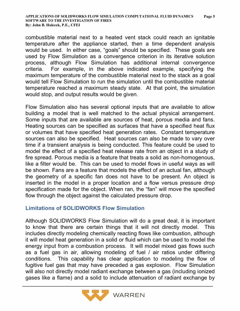
an absorbing medium such as water vapor. However, it will model radiant exchange between solids, and a flame could potentially be modeled as a radiating solid at a certain internal heat generation rate or temperature. The practical effect of these limitations varies depending on the problem under analysis. The best way to show the application of the software is by reference to an example. Flow Simulation Example 1: A Burner in a Wooden Box, Modeling a Gas Burner One question that arises in fire investigation is if a heat producing appliance (e.g. furnace, gas fireplace) created sufficiently high temperatures in adjacent combustibles to ignite a fire. Frequently such appliances use fuel gas fired burners. To refine the usage of SOLIDWORKS Flow Simulation to examining such questions, a test apparatus with gas burner was constructed and outfitted with multiple temperature sensors. The goal of the testing was to determine if Flow Simulation could be used to accurately simulate heating from a gas burner despite Flow Simulation not directly modeling combustion. The apparatus, shown in figure 1, consisted of a propane fueled tube burner mounted inside a plywood box. The burner was equipped with a #56 orifice and supplied at 2.6-2.7kPa (10.5-11.0 inwc) pressure propane gas. Openings were included near floor level and in the top of the box. The CFD model was ran as an external analysis which includes the environment around the box. Flow was allowed into and out of the openings of the box under the influence of the buoyant effects of gravity due to the burner heat. Conduction within solids was allowed as was convection to the walls. Convective heat transfer coefficients were calculated using the methodology of Section 7-9 of JP Holman’s Heat Transfer text.3 These ranged from 2.1-5.8 W/m2K (0.37-1.02 BTU/HrFT2F) for the differing surfaces. External air temperatures were set at 26.7°C (80°F), which was the temperature in the lab. Radiation was not included in this model, as the relatively “clean” flame had a comparatively low proportion of energy emitted as radiant heat. Additionally, essentially all the energy released as radiant heat would transfer to the box interior surfaces as the openings in the box were small. As shown in figure 2, the burner was modeled by creating a solid representation of the “flame” in the approximate size of the actual flame. The


Page 7

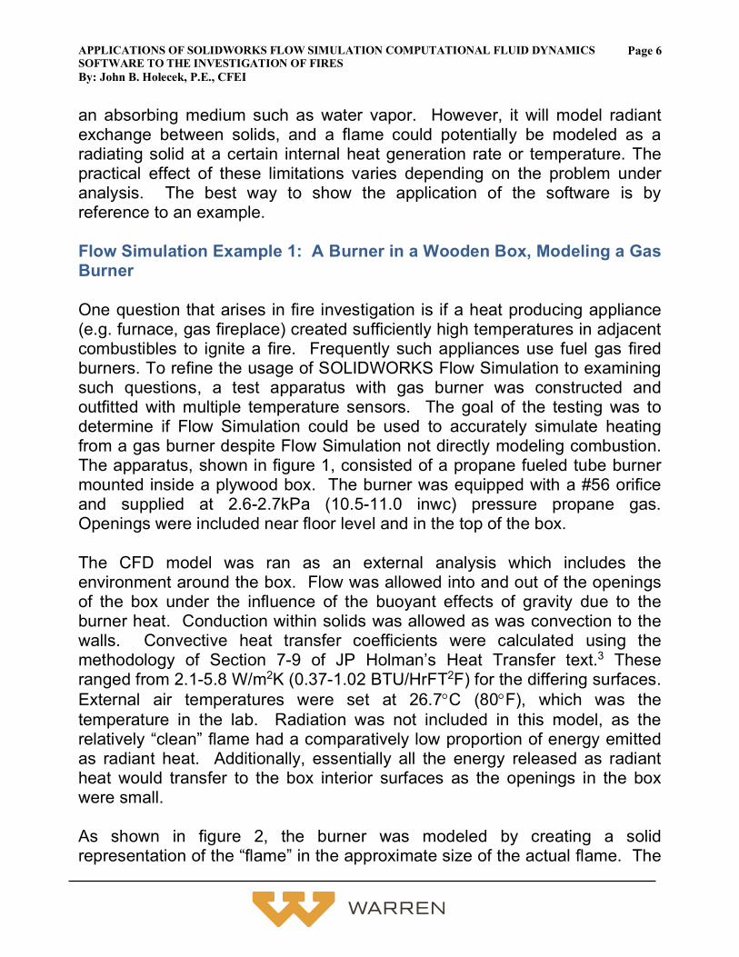
solid “flame” was made porous and given an internal heat generation rate equal to the associated lower heating value of propane for the measured flowrate of fuel. The flame was connected or “mated” to a model of the tube burner which included the burner ports. Normally, a discharge of LP gas from the burner orifice entrains air into the burner’s venturi and the combined mixture discharged from the ports. To simulate this process, a “fan” was used to model flow through the burner. In Flow Simulation, “fans” are features of a model that act as a real fan does, moving volume and/or mass at a defined rate. In this case, a fan was added that moved a mass of air equal to the stoichiometrically correct volume for the gas flow measured during the test.

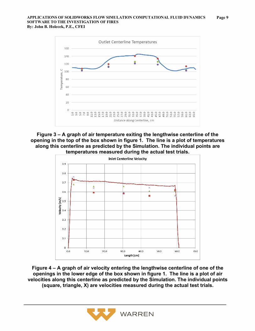
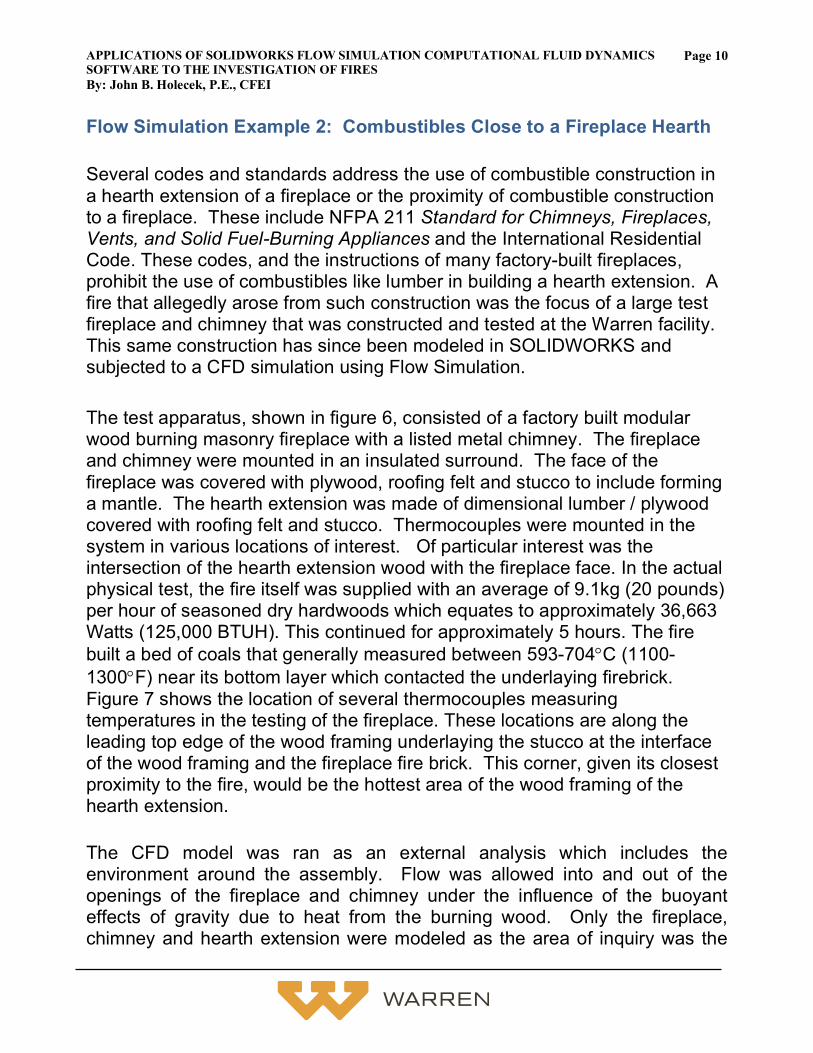
As shown in figures 3-5, the model had a reasonably close agreement with measured temperatures and velocities. For example, referencing figure 3 predicted versus measured exiting air temperatures at the top slot ranged from essentially exact agreement to a maximum difference of 21°C (121°C versus 142°C). This is a range of 0-5.3% calculated as the difference between actual and predicted values over the value of the actual temperature in absolute units (degrees Kelvin). Referencing figure 4, predicted versus measured inlet velocity varied from essential agreement to a maximum difference of 0.13 m/s (.59 to .72 m/s). This is a range of 0-22% difference calculated as the velocity difference divided by the actual value. Referencing figure 5, the single interior top surface that was monitored averaged 112°C while the predicted temperature was 113°C on one side of the slot and 98°C on the other side, a difference of 0% to 3.6% depending on what side is considered and calculated as the difference between actual and predicted values over the value of the actual temperature in absolute units (degrees Kelvin).


Page 8

Figure 1 – Flow Modeling Test Apparatus of a Wooden Box with an Internal Burner. The Corresponding Solid Model is Shown to the Right.

Figure 2 – Solid Model of the Burner Showing Several Features and the Airflow Due

to the “Fan” Feature.

“Flame”, Modeled as a Porous Material with a

Specified Heat Generation rate. The porous media

allows airflow from the “fan” to discharge through the

“flame”

SOLIDWORKS “Fan” inside burner tube specified to have

mass flowrate equal to the stoichiometrically correct quantity of airflow for the

quantity of gas burned.


Page 9

Figure 3 – A graph of air temperature exiting the lengthwise centerline of the

opening in the top of the box shown in figure 1. The line is a plot of temperatures along this centerline as predicted by the Simulation. The individual points are

temperatures measured during the actual test trials.

Figure 4 – A graph of air velocity entering the lengthwise centerline of one of the openings in the lower edge of the box shown in figure 1. The line is a plot of air

velocities along this centerline as predicted by the Simulation. The individual points (square, triangle, X) are velocities measured during the actual test trials.


Page 10

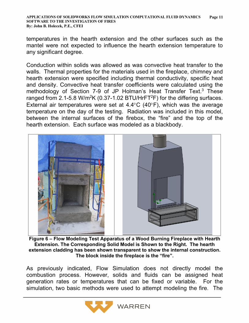
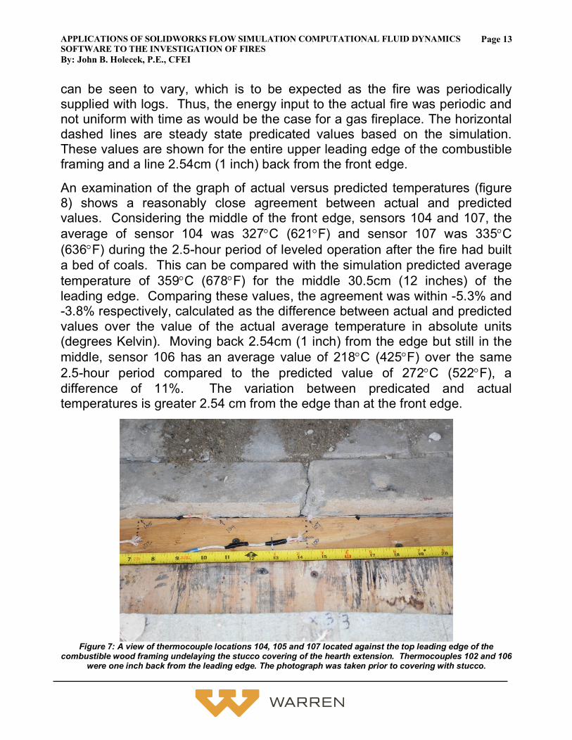
Flow Simulation Example 2: Combustibles Close to a Fireplace Hearth Several codes and standards address the use of combustible construction in a hearth extension of a fireplace or the proximity of combustible construction to a fireplace. These include NFPA 211 Standard for Chimneys, Fireplaces, Vents, and Solid Fuel-Burning Appliances and the International Residential Code. These codes, and the instructions of many factory-built fireplaces, prohibit the use of combustibles like lumber in building a hearth extension. A fire that allegedly arose from such construction was the focus of a large test fireplace and chimney that was constructed and tested at the Warren facility. This same construction has since been modeled in SOLIDWORKS and subjected to a CFD simulation using Flow Simulation. The test apparatus, shown in figure 6, consisted of a factory built modular wood burning masonry fireplace with a listed metal chimney. The fireplace and chimney were mounted in an insulated surround. The face of the fireplace was covered with plywood, roofing felt and stucco to include forming a mantle. The hearth extension was made of dimensional lumber / plywood covered with roofing felt and stucco. Thermocouples were mounted in the system in various locations of interest. Of particular interest was the intersection of the hearth extension wood with the fireplace face. In the actual physical test, the fire itself was supplied with an average of 9.1kg (20 pounds) per hour of seasoned dry hardwoods which equates to approximately 36,663 Watts (125,000 BTUH). This continued for approximately 5 hours. The fire built a bed of coals that generally measured between 593-704°C (1100-1300°F) near its bottom layer which contacted the underlaying firebrick. Figure 7 shows the location of several thermocouples measuring temperatures in the testing of the fireplace. These locations are along the leading top edge of the wood framing underlaying the stucco at the interface of the wood framing and the fireplace fire brick. This corner, given its closest proximity to the fire, would be the hottest area of the wood framing of the hearth extension.

The CFD model was ran as an external analysis which includes the environment around the assembly. Flow was allowed into and out of the openings of the fireplace and chimney under the influence of the buoyant effects of gravity due to heat from the burning wood. Only the fireplace, chimney and hearth extension were modeled as the area of inquiry was the


Page 11

temperatures in the hearth extension and the other surfaces such as the mantel were not expected to influence the hearth extension temperature to any significant degree. Conduction within solids was allowed as was convective heat transfer to the walls. Thermal properties for the materials used in the fireplace, chimney and hearth extension were specified including thermal conductivity, specific heat and density. Convective heat transfer coefficients were calculated using the methodology of Section 7-9 of JP Holman’s Heat Transfer Text.3 These ranged from 2.1-5.8 W/m2K (0.37-1.02 BTU/HrFT2F) for the differing surfaces. External air temperatures were set at 4.4°C (40°F), which was the average temperature on the day of the testing. Radiation was included in this model, between the internal surfaces of the firebox, the “fire” and the top of the hearth extension. Each surface was modeled as a blackbody.

Figure 6 – Flow Modeling Test Apparatus of a Wood Burning Fireplace with Hearth

Extension. The Corresponding Solid Model is Shown to the Right. The hearth extension cladding has been shown transparent to show the internal construction.

The block inside the fireplace is the “fire”. As previously indicated, Flow Simulation does not directly model the combustion process. However, solids and fluids can be assigned heat generation rates or temperatures that can be fixed or variable. For the simulation, two basic methods were used to attempt modeling the fire. The


Page 12

first method was to create a solid object of approximately the same size as the combined burning logs and bed of coals and ascribe to that object an internal volumetric heat generation rate equal to the average energy input of 36,663 Watts (125,000 BTUH). The second method was to create a solid object of the size of the bed of coals and ascribe to it the average 649°C (1200°F) temperature of the bed of coals as measured in the test. Several simulations were ran using the volumetric heat generation rate method. Generally, the method tended to overestimate the temperature of the “fire” when the modeled volume was of a physical size approximating the visual volume of the burning logs and bed of coals. This is likely because it confines the energy release occurring in the reacting flame into the smaller volume of the logs and coals. In short, the surface area of the modeled solid through which the specified energy must be emitted was so small as to require a higher temperature difference to transfer the heat than occurs in normal combustion. If this volumetric heat generation method is used to model a fire, it would be necessary to have a sufficiently large volume such that the temperature of the volume drops to a normal flame temperature for the actual situation at hand. Further work may show this method can be successfully employed at a sufficiently large volume. The second method employed was to fix the temperature of the volume representing the coals and logs at the average 649°C (1200°F) temperature of the bed of coals as measured in the test. A practical use of the simulation was to determine if combustible construction in the hearth extension was exposed to temperatures sufficient to result in ignition. Examination of the geometry of the wood hearth structure construction makes it apparent that conduction heat transfer from the adjacent fire brick and hearth extension stucco covering would be the dominate form of heat transfer to the underlaying combustible material. On this basis, for the specific purpose of modeling the temperature of the combustible hearth extension framing, the overall heat generation rate of the fire, mostly lost as convective heating of air and radiant heat to the environment, was considered less of a significant input as compared to the known temperature of the bed of coals. This fixed method appeared to have better promise as a means of modeling the fire for this specific purpose.

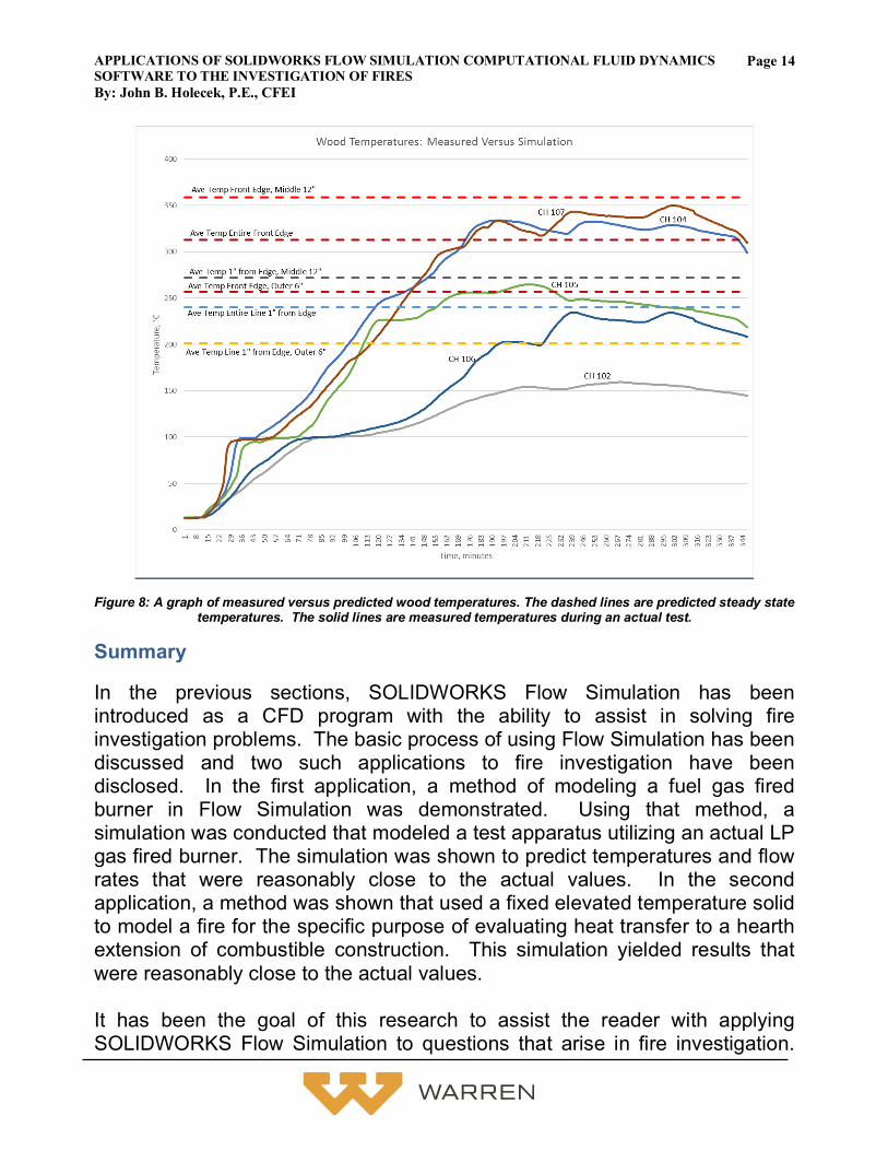
A comparison of the simulation data with temperatures recorded in the test is shown in figure 8. The solid lines that increase from the left are actual temperatures recorded in the physical test, increasing with time. The values


Page 13

can be seen to vary, which is to be expected as the fire was periodically supplied with logs. Thus, the energy input to the actual fire was periodic and not uniform with time as would be the case for a gas fireplace. The horizontal dashed lines are steady state predicated values based on the simulation. These values are shown for the entire upper leading edge of the combustible framing and a line 2.54cm (1 inch) back from the front edge.

An examination of the graph of actual versus predicted temperatures (figure 8) shows a reasonably close agreement between actual and predicted values. Considering the middle of the front edge, sensors 104 and 107, the average of sensor 104 was 327°C (621°F) and sensor 107 was 335°C (636°F) during the 2.5-hour period of leveled operation after the fire had built a bed of coals. This can be compared with the simulation predicted average temperature of 359°C (678°F) for the middle 30.5cm (12 inches) of the leading edge. Comparing these values, the agreement was within -5.3% and -3.8% respectively, calculated as the difference between actual and predicted values over the value of the actual average temperature in absolute units (degrees Kelvin). Moving back 2.54cm (1 inch) from the edge but still in the middle, sensor 106 has an average value of 218°C (425°F) over the same 2.5-hour period compared to the predicted value of 272°C (522°F), a difference of 11%. The variation between predicated and actual temperatures is greater 2.54 cm from the edge than at the front edge.

Figure 7: A view of thermocouple locations 104, 105 and 107 located against the top leading edge of the

combustible wood framing undelaying the stucco covering of the hearth extension. Thermocouples 102 and 106 were one inch back from the leading edge. The photograph was taken prior to covering with stucco.


Page 14

Figure 8: A graph of measured versus predicted wood temperatures. The dashed lines are predicted steady state

temperatures. The solid lines are measured temperatures during an actual test.

Summary

In the previous sections, SOLIDWORKS Flow Simulation has been introduced as a CFD program with the ability to assist in solving fire investigation problems. The basic process of using Flow Simulation has been discussed and two such applications to fire investigation have been disclosed. In the first application, a method of modeling a fuel gas fired burner in Flow Simulation was demonstrated. Using that method, a simulation was conducted that modeled a test apparatus utilizing an actual LP gas fired burner. The simulation was shown to predict temperatures and flow rates that were reasonably close to the actual values. In the second application, a method was shown that used a fixed elevated temperature solid to model a fire for the specific purpose of evaluating heat transfer to a hearth extension of combustible construction. This simulation yielded results that were reasonably close to the actual values. It has been the goal of this research to assist the reader with applying SOLIDWORKS Flow Simulation to questions that arise in fire investigation.


Page 15

Whereas these two simulations yielded reasonably close agreement between actual and predicted values, the extension of these methods to alternative simulations should be undertaken with care. As with any use of a simulation, careful consideration should be given to defining the problem, selecting the candidate model and model verification and validation. The use of simulations in fire investigation should be within the framework outlined in NFPA 921, which can be consulted for additional information.4

Endnotes

1. Ivanov, Trebunskikh, Platonovich: “Validation Methodology for Modern CAD-Embedded CFD Code: from Fundamental Tests to Industrial Benchmarks”. SolidWorks White Paper (2014)

2. Technical Reference, SOLIDWORKS Flow Simulation 2017, Dassault Systemes (2017)

3. Holman, JP, Heat Transfer, McGraw-Hill Book Company, New York (1981)

4. NFPA 921 Guide for Fire and Explosion Investigations, National Fire Protection Association, (2017)

About the Author John Holecek, senior consulting engineer at Warren, is a licensed professional engineer in 8 states and has both a Bachelor of Science in Mechanical Engineering and Master of Science in Mechanical Engineering from the University of South Carolina. A certified fire and explosion investigator by the national Associate of Fire Investigators, John has more than 23 years experience in the design of industrial process equipment and is extremely knowledgeable in ICC, NFPA and OSHA codes and standards. He pairs more than 13 years experience supervising manufacturing operations with deep knowledge in areas such as applied industrial heat transfer in oven design, industrial electrical process and motor control systems, material handling systems and fire protection systems. In addition, he’s designed paint finishing systems, and commercial and consumer gas fired cooking appliances. John has managed outside contractors in site safety requirements and installation of industrial process equipment. By virtue of his experience, he is well versed in federal and state worker safety regulations.

Documents

APPLICATIONS OF SOLIDWORKS FLOW SIMULATION … · applications of solidworks flow simulation computational fluid dynamics software to the investigation of fires by: john b. holecek,