Applications of Raman Spectroscopy

and Chemometrics to Semiconductor

Process Control

A thesis for the degree o f

Master of Science

Subm itted to

Dublin C ity University

By

Ian Robertson B.Sc.

R esearch Supervisor

D r Enda M cG lynn

School of Physical Sciences

D ublin C ity University

A ugust 2000

Declaration

I hereby certify that this material, which I now submit for assessment on the

program of study leading to the award of Master of Science is entirely my own work

and has not been taken from the work of others save and to the extent that such work

has been cited and acknowledged within the text of my work.

Signed:_ / j - a i J L ~ ID No: 97970301Ian Robertson

Date: rs AA<

ii

Table of Contents

Title Page iDeclaration i iTable of Contents i i iAcknowledgements vAbstract v i

Chapter 1: Introduction

1.1 Introduction 11.2 The Standard Clean (SC-1) Solution 21.3 SC-1 Compositional Analysis 41.4 Raman Spectroscopy and Chemometrics 6

Chapter 2: Spectroscopic Methods and Sample Preparation

2.1 Introduction 82.1.1 Raman Scattering 8

2.2 Classical Theory of Raman Scattering 102.3 Quantum Theory of Raman S cattering 122.4 Kaiser Holoprobe Integrated Fibre-Coupled Raman System 15

2.4.1 System Overview 152.4.2 Holographic Optics 15

2.4.2.1 Holographic Gratings 162.4.2.2 Holographic Filters 172.4.2.3 The Axial Transmission Spectrograph 18

2.4.3 Helium-Neon Laser 192.4.4 CCD Camera 192.4.5 Fibre-Optic Probe 20

2.5 Sample Preparation 222.6 Titrations 23

2.6.1 Hydro gen Peroxide 242.6.2 Ammonium Hydroxide 24

2.7 Sample Holder 252.8 System Set-up 25

Chapter 3: Chemometrics

3.1 Introduction 273.2 Univariate Analysis 27

3.2.1 Least Squares Regression 283.3 Multivariate Analysis: An Example 30

3.3.1 Introduction to Multivariate Analysis 3 3

iii

3.3.2 Principal Components Analysis 363.3.2.1 Geometrie Interpretation of Principal 3 7

Components Analysis3.3.3 Chemometrics Software 39

3.4 Conclusion 39

Chapter 4: Data Analysis

4.1 Introduction 404.1.1 Raman Spectrum of SC-1 Solution 41

4.2 Univariate Analysis of Raman Spectra 424.3 Multivariate Analysis 43

4.3.1 Regression Coefficients 434.3.2 Calibration 1 45

4.3.2.1 Percentage Models, Hydrogen Peroxide 454.3.2.2 Ammonium Hydroxide 484.3.2.3 Molar Models, Hydrogen Peroxide 494.3.2.4 Ammonium Hydroxide 51

4.3.3 Calibration 2 534.3.3.1 Percentage Models, Hydrogen Peroxide 534.3.3.2 Ammonium Hydroxide 554.3.3.3 Molar Models, Hydrogen Peroxide 564.3.3.4 Ammonium Hydroxide 58

4.3.4 Water Calibration 594.4 Conclusion 60

Chapter 5: Discussion and Conclusions 62

Bibliography 65

Appendix A A-lAppendix B B-l

i v

Acknowledgements

I would like to thank my supervisor Dr Enda McGlynn for the opportunity to

pursue research within this group. I thank Enda for his patience, encouragement and

guidance throughout the course of this project. I would also like to thank Prof. Brian

MacCraith for his help on different aspects of the research and the Chemistry

department for their help at various stages.

I am grateful to my colleagues at DCU who made my time here very

enjoyable and interesting, in particular Mark, Cathal, Jason, Clodagh, Eilish, Kieran,

Pat and Roisin. A special thanks goes to the technical staff at the Physics

department. Des and Al, I am very grateful. To Louise, thanks for the

encouragement.

Finally, I would like to dedicate this thesis to my parents, George and Esther,

for their unwavering support, understanding and patience.

Abstract

The Standard Clean (SC-1) solution, which contains a mixture of hydrogen

peroxide (H2O2), ammonium hydroxide (NH4OH) and water, makes up the most

important part in the RCA cleaning process for semiconductor wafers. This step has

proven to be the most effective method for the removal of contaminants.

The SC-1 solution is, however, very unstable due to the decomposition of

H2O2 and the evaporation of NH4OH. This work aims to use a combination of

Raman spectroscopy and chemometrics in order to predict the concentrations of the

individual components of unknown samples of SC-1. The attraction of such a

technique is that it is non-invasive and therefore can be performed on-line. The

potential cost-savings for semiconductor manufacturers are also considerable.

Both calibration and prediction sets were obtained for various concentrations

of SC-1 solutions. The results of the analyses performed are presented here.

v i

Chapter 1

Introduction

1.1 Introduction

The requirement for clean semiconductor wafers is becoming more and

more important as semiconductor device geometries continue to shrink and die

sizes grow. Such developments mean that microcontaminants such as particles and

metallic impurities will have an ever-increasing detrimental impact on device yield

and reliability.

Wet chemical processing has been widely used as a major cleaning tool in

ultra large scale integration (ULSI) manufacturing and the current wet cleaning

process for silicon wafers is based on the so called Radio Corporation of America

(RCA) cleaning method introduced by Kern and Puotien in 1 9 7 0 One of the steps

involved in the RCA process is the Standard Clean (SC-1), which contains a

mixture of hydrogen peroxide (H2O2), ammonium hydroxide (NH4OH), and water.

This step has proven to be the most successful method for the removal of particles

since it was first developed nearly thirty years ago, and has, therefore, become the

most important cleaning technique in the manufacture of sub-micron devices/ 21

The SC-1 solution is, however, notoriously unstable due to H2O2

decomposition and evaporative losses of NH3 and water.[3] The SC-1 composition

shows considerable variation over time and is almost impossible to predict.

Although in use for nearly thirty years little has been done in an attempt to control

the chemical concentrations of the processing baths. Such concentration control is

]

essential for more uniform processing, chemical cost reduction, productivity

enhancements, and for environmental reasons.

The purpose of this project was to develop a non-invasive technique for the

prediction of the individual component concentrations of SC-1 using Raman

spectroscopy in conjunction with chemometric techniques.

1.2 The Standard Clean (SC-1) Solution

The SC-1 solution consists of a mixture of ammonium-hydroxide,

hydrogen-peroxide and water. The mixture has also been referred to as APM

(Ammonium Hydroxide-Hydrogen Peroxide Mixture. This solution has been found

to be the most efficient particle removal agent to date.[4] SC-1 solutions facilitate

particle removal by etching the wafer underneath the particles; thereby loosening

the particles, so that mechanical forces can readily remove the particles from the

wafer surface. Megasonic energy can further aid particle removal through

cavitation (bubble formation) and/or acoustic streaming (fluid motion).[5'7] The

ammonium hydroxide in the solution steadily etches silicon dioxide at the boundary

between the oxide and the aqueous solution (i.e., the wafer surface). The hydrogen

peroxide in SC-1 serves to protect the surface from attack by OH’ by re-growing a

protective oxide directly on the silicon surface (i.e., at the silicon/oxide interface).

If sufficient hydrogen peroxide is not present in the solution, the silicon will be

anisotropically etched and surface roughening quickly ensues. This surface

roughening can adversely affect gate oxide breakdown. Conversely, hydrogen

peroxide is known to readily dissociate and form water and oxygen. With such

dissociation, bubbles can appear in the solution if the concentration of oxygen is too

high. The gas-liquid interfaces that result from the formation of such bubbles can

2

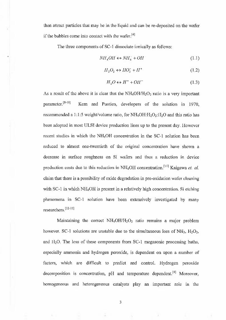
then attract particles that may be in the liquid and can be re-deposited on the wafer

if the bubbles come into contact with the wafer.141

The three components of SC-1 dissociate ionically as follows:

NH,OH <-> NH+ + OH~ (1.1)

H 20 2 <^H 0- + H + (1.2)

H 20 < ^ H + +OH~ (1.3)

As a result of the above it is clear that the NH4OH/H2O2 ratio is a very important

parameter/8"10 Kern and Puotien, developers of the solution in 1970,

recommended a 1:1:5 weight/volume ratio, for NH40H:H202:H20 and this ratio has

been adopted in most ULSI device production lines up to the present day. However

recent studies in which the NH4OH concentration in the SC-1 solution has been

reduced to almost one-twentieth of the original concentration have shown a

decrease in surface roughness on Si wafers and thus a reduction in device

production costs due to this reduction in NH4OH concentration.[11] Kaigawa el. al.

claim that there is a possibility of oxide degradation in pre-oxidation wafer cleaning

with SC-1 in which NH4OH is present in a relatively high concentration. Si etching

phenomena in SC-1 solution have been extensively investigated by many

researchers. [12'15]

Maintaining the correct NH4OH/H2O2 ratio remains a major problem

however. SC-1 solutions are unstable due to the simultaneous loss of NH3, H2O2,

and H2O. The loss of these components from SC-1 megasonic processing baths,

especially ammonia and hydrogen peroxide, is dependent on upon a number of

factors, which are difficult to predict and control. Hydrogen peroxide

decomposition is concentration, pH and temperature dependent.M oreover,

homogeneous and heterogeneous catalysts play an important role in the

3

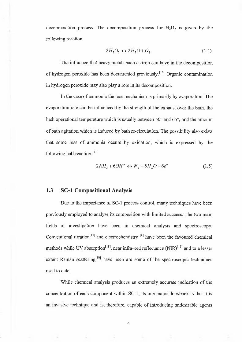
decomposition process. The decomposition process for H2O2 is given by the

following reaction.

2H20 2 <-> 2H20 + 0 2 (1.4)

The influence that heavy metals such as iron can have in the decomposition

of hydrogen peroxide has been documented previously.[16] Organic contamination

in hydrogen peroxide may also play a role in its decomposition.

In the case of ammonia the loss mechanism is primarily by evaporation. The

evaporation rate can be influenced by the strength of the exhaust over the bath, the

bath operational temperature which is usually between 50° and 65°, and the amount

of bath agitation which is induced by bath re-circulation. The possibility also exists

that some loss of ammonia occurs by oxidation, which is expressed by the

following half reaction.[4]

2NH3 +60H- < ^N 2 + 6H20 + 6e~ (1.5)

1.3 SC-1 Com positional Analysis

Due to the importance of SC-1 process control, many techniques have been

previously employed to analyse its composition with limited success. The two main

fields of investigation have been in chemical analysis and spectroscopy.

Conventional titration 171 and electrochemistry [4] have been the favoured chemical

methods while UV absorption[18], near infra-red reflectance (NIR)[11] and to a lesser

extent Raman scattering 191 have been are some of the spectroscopic techniques

used to date.

While chemical analysis produces an extremely accurate indication of the

concentration of each component within SC-1, its one major drawback is that it is

an invasive technique and is, therefore, capable of introducing undesirable agents

4

which add to the complexity of the solution and also necessitate the need for

frequent re-calibration. Furthermore, they are not well suited to on-line process

control or any level of automation as frequently the process must be shut down in

order to facilitate such measurements. Spectroscopic techniques can be applied

non-invasively, but on the other hand, they have their limitations; an example being

that UV absorption cannot detect NH4OHJ20'

Mid-infrared spectroscopy, usually in the form of Fourier Transform

Infrared (FTIR), is a widely used optical spectroscopic technique. Its advantages

are that it produces data with good S/N consisting of sharp peaks that are readily

identifiable with each chemical component. These peak areas can then be directly

converted into numerical concentration values. However there are significant

problems associated with the sampling process that restrict FTIR's usefulness in this

application. These measurements require very short path lengths (10|un or less) and

secondly the high absorbances can sometimes distort the linear relationship

between the measured signal and the actual concentration.[20]

On the other hand, NIR (near infrared) spectroscopy can be used non-

invasively; the NIR light being directed through a glass vial or cell, with either of

the transmitted or reflected signals being recorded. However, the convoluted nature

of the data returning requires that the instrument's software be calibrated on a large

number of reference samples. Any minor change introduced in the process

(particularly temperature) requires a complete re-calibration of the system. Also,

both NIR and FTIR techniques can sometimes have difficulties with aqueous

samples because of the strong water signals that are returned. Nevertheless there

has been some success with NIR spectroscopy in Japan recently.[2I]

5

1.4 Ram an Spectroscopy and Chem om etrics

The approach taken in this project was to use Raman spectroscopy coupled

with chemometrics for the non-invasive quantitative analysis of SC-1. Raman

spectroscopy has been shown to be excellent for the identification of atomic and

molecular species. The use of Raman spectroscopy up until recently, however, was

confined to research laboratories due to the need for high powered lasers with water

cooled power supplies and the need for high performance double monochromators.

When one considers such requirements coupled with a relatively weak Raman

scattering signals from most samples it is possible to envisage why such a

technique had found little usage within industry. However within the last decade a

number of technologies have combined to ensure that Raman systems are now

much more portable and compact than before. The advent of CCD detectors,

compact solid state lasers, holographic filters and fibre optic laser light delivery

have exposed Raman spectroscopy to a much broader base of applications,

especially within the microelectronics, chemical, pharmaceutical, food and

biomedical industries. Some other applications for Raman spectroscopy have been

found in:

• the characterisation of diamond like carbon filrtW221

• measurement of degree of polymerisation 231

• pharmaceutical industry 241

• silicon stress analysis 251

• petroleum Analysis126,271

Considering how much Raman technology has advanced in recent years it becomes

clear why it is now an excellent process control technique, and is ideally suited to

the current application. Also Raman spectroscopy gives very sharp well-defined

6

peaks in the SC-1 application. This is advantageous when analysing these spectra

with both univariate and multivariate analysis techniques.

7

Chapter 2

Spectroscopic Methods and Sample Preparation

2.1 Introduction

The theory behind Raman Scattering is developed in this chapter. Although

not a completely rigorous description, the fundamentals of both the classical and

quantum mechanical formulations are discussed. Following this, an outline of the

Kaiser Optical System's Holoprobe used in this project is given, and its

specifications are described.

2.1.1 Raman Scattering

The Raman effect was first predicted by Smekal128' in 1923 but it wasn't

until 1928 that it was experimentally observed by Chandresekhara Venkata Raman,

an Indian physicist 331 who was later awarded the Nobel Prize for his discovery.

Smekal predicted that radiation scattered from molecules not only contains

photons with the incident photon frequency but also photons with a change in

frequency. It is exactly this phenomenon that describes the Raman effect.

The Raman effect can be described as the inelastic scattering of light by

matter. When a photon of light, too low in energy to excite an electronic transition

from one state to another, strikes a molecule, it can be scattered in one of three

different ways. Firstly the incident photon can be scattered elastically, i.e. the

incident photon energy is the same as the scattered photon energy. This is also

8

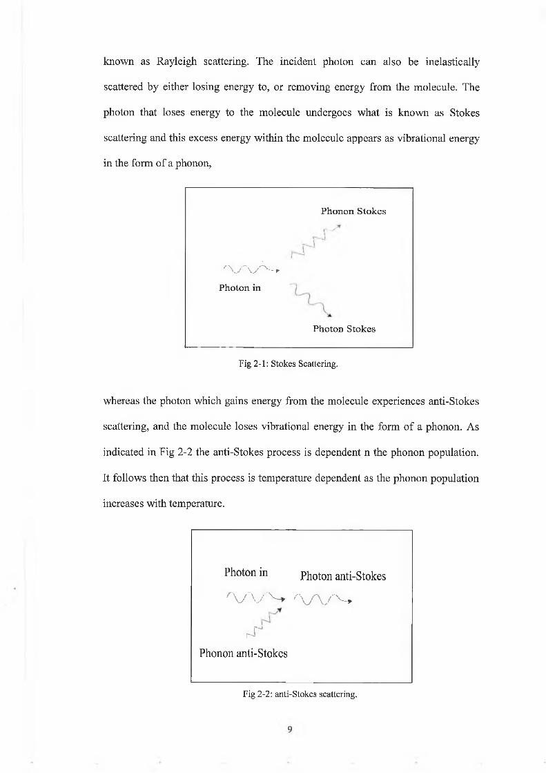
known as Rayleigh scattering. The incident photon can also be inelastically

scattered by either losing energy to, or removing energy from the molecule. The

photon that loses energy to the molecule undergoes what is known as Stokes

scattering and this excess energy within the molecule appears as vibrational energy

in the form of a phonon,

Phonon Stokes

,r\ y \ y ' N—►Photon in

Photon Stokes

Fig 2-1: Stokes Scattering.

whereas the photon which gains energy from the molecule experiences anti-Stokes

scattering, and the molecule loses vibrational energy in the form of a phonon. As

indicated in Fig 2-2 the anti-Stokes process is dependent n the phonon population.

It follows then that this process is temperature dependent as the phonon population

increases with temperature.

Photon in Photon anti-Stokes

r \ r \ r ^ * r \ / \ r - ~ +

v TPhonon anti-Stokes

Fig 2-2: anti-Stokes scattering.

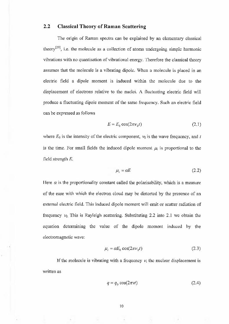
The origin of Raman spectra can be explained by an elementary classical

theory[29], i.e. the molecule as a collection of atoms undergoing simple harmonic

vibrations with no quantisation of vibrational energy. Therefore the classical theory

assumes that the molecule is a vibrating dipole. When a molecule is placed in an

electric field a dipole moment is induced within the molecule due to the

displacement of electrons relative to the nuclei. A fluctuating electric field will

produce a fluctuating dipole moment of the same frequency. Such an electric field

can be expressed as follows

E = E0 cos(2n;v0t) (2.1)

where Eq is the intensity of the electric component, Vo is the wave frequency, and t

is the time. For small fields the induced dipole moment ju\ is proportional to the

field strength E.

- aE (2.2)

Here a is the proportionality constant called the polarisability, which is a measure

of the ease with which the electron cloud may be distorted by the presence of an

external electric field. This induced dipole moment will emit or scatter radiation of

frequency Vo. This is Rayleigh scattering. Substituting 2.2 into 2.1 we obtain the

equation determining the value of the dipole moment induced by the

electromagnetic wave:

//,. = aE0 cos(27rv0t) (2.3)

If the molecule is vibrating with a frequency v, the nuclear displacement is

written as

q = q0 cos(2nvt) (2.4)

2.2 C lassical Theory o f R am an Scattering

1 0

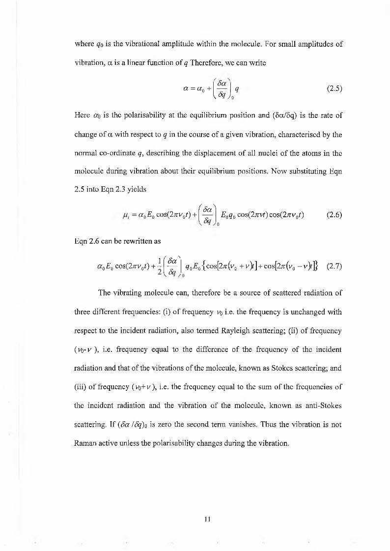
where qo is the vibrational amplitude within the molecule. For small amplitudes of

vibration, a is a linear function of q Therefore, we can write

a = a 0 + (2.5)v ^ y 0

Here ao is the polarisability at the equilibrium position and (5a/8q) is the rate of

change of a with respect to q in the course of a given vibration, characterised by the

normal co-ordinate q, describing the displacement of all nuclei of the atoms in the

molecule during vibration about their equilibrium positions. Now substituting Eqn

2.5 into Eqn 2.3 yields

= a 0E0 cos(27rv0t) +

Eqn 2.6 can be rewritten as

r 5 a ' E0q0 cos(2n:vt)cos(27rv0t) (2.6)

_ 1 ( S a 'a 0E0 cos(27rv0t) + - — q0E0 {cos[2^r(v0 + v)i] + cos[2;r(v0 - v)/]} (2.7)

The vibrating molecule can, therefore be a source of scattered radiation of

three different frequencies: (i) of frequency Vo i-e. the frequency is unchanged with

respect to the incident radiation, also termed Rayleigh scattering; (ii) of frequency

(vo-v ), i.e. frequency equal to the difference of the frequency of the incident

radiation and that of the vibrations of the molecule, known as Stokes scattering; and

(iii) of frequency ( v q + v ), i.e. the frequency equal to the sum of the frequencies of

the incident radiation and the vibration of the molecule, known as anti-Stokes

scattering. If (Sa /Sq)o is zero the second term vanishes. Thus the vibration is not

Raman active unless the polarisability changes during the vibration.

1 1

Electromagnetic radiation exhibits the properties of both a stream of

particles and a wave. Therefore the Raman effect can be described in two ways.

The previous interpretation is based on wave theory, which was the classic

approach to electromagnetic radiation. However the quantum mechanical approach

recognises the fact that the vibrational energy of a molecule is quantised showing

particulate nature, and such particles are generally known as quanta. In the case of

electromagnetic radiation they are also known as photons. The relationship between

the energy £ o f a photon and its frequency is described by the Planck formula:

E = hv (2.8)

The interaction of the photon with the molecule can yield three phenomena:

absorption, emission and scattering. It is obviously scattering that interests us in the

case of Raman spectroscopy. Scattering takes place within 10'14s of when a photon,

of energy not equal to the energy difference between any two stationary levels of

the molecule, interacts with that molecule.

The normal Raman effect takes place when a photon, with an energy

distinctly lower than that of the energy difference between the ground level and the

first excited state, interacts with a molecule.

Scattering is a two-photon process^30, 311 that cannot be separated

experimentally into two single photon steps of absorption and emission. The photon

with an initial energy of hvo can (a) proceed without a change in energy (otherwise

known as Rayleigh scattering), (b) experience a decrease in energy hvk(st)(Stokes

scattering), or (c) experience an increase in energy h vR(aSt) (anti-Stokes scattering).

Fig 2-3 illustrates what happens when identical molecules are illuminated with

monochromatic light.[33] The resulting spectrum is also shown.

2.3 Quantum Theory o f Ram an Scattering

1 2

Fig 2-3: (a) Diagram o f scattering during illumination with monochromatic light, (b) Part o f the resulting spectrum, where \iRny is the Rayleigh Scatter, Vk(s o 's the Raman Stokes Scatter, is the Raman anti-Stokes scatter, and vv is one o f the possible vibrational frequencies o f the molecule.

Two electronic levels are shown. Ground state level (0) and the first excited

state (1). The vibrational levels are also illustrated. The dashed lines depict two

virtual levels of the molecule, separated by hvw where vv is one of the possible

vibrations of the molecule. According to the Boltzmann law, most of the molecules

will occupy the vibrational ground state at room temperature. This is why Stokes

1 3

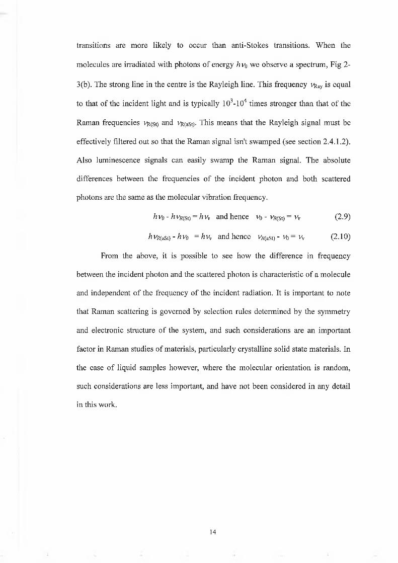
transitions are more likely to occur than anti-Stokes transitions. When the

molecules are irradiated with photons of energy hvo we observe a spectrum, Fig 2-

3(b). The strong line in the centre is the Rayleigh line. This frequency vfcay is equal

to that of the incident light and is typically 103-104 times stronger than that of the

Raman frequencies v (st) and vfc(ast)- This means that the Rayleigh signal must be

effectively filtered out so that the Raman signal isn't swamped (see section 2.4.1.2).

Also luminescence signals can easily swamp the Raman signal. The absolute

differences between the frequencies of the incident photon and both scattered

photons are the same as the molecular vibration frequency.

hvo - hVr(si) = hvv and hence Vo - vft(st) = vv (2.9)

h vft(ast) - h Vo = hvv and hence v«(ast) - H) = vv (2 .10)

From the above, it is possible to see how the difference in frequency

between the incident photon and the scattered photon is characteristic of a molecule

and independent of the frequency of the incident radiation. It is important to note

that Raman scattering is governed by selection rules determined by the symmetry

and electronic structure of the system, and such considerations are an important

factor in Raman studies of materials, particularly crystalline solid state materials. In

the case of liquid samples however, where the molecular orientation is random,

such considerations are less important, and have not been considered in any detail

in this work.

1 4

2.4 Kaiser Holoprobe Integrated Fibre Coupled Raman System

The various parts that make up the Kaiser Holoprobe Raman system used in

this project are outlined below.

2.4.1 System Overview

Shown below in Fig 2-4 is an outline of the Kaiser Optical Holoprobe

Raman system. Holographic optics, the probe head and the CCD camera are of

particular interest in terms of the modem Raman instrument. These allow for much

quicker Raman data collection.

Fig 2-4: Outline o f Kaiser Raman system

2.4.2 Holographic Optics

The Kaiser Holoprobe embraces all the recent technologies that make up the

modern Raman instrument. The emergence of holographic optics has been central

to the development of portable Raman systems. The Holoprobe uses volume phase

holograms for both filtering and dispersion functions. The advantages of such

holograms are manifold. They provide a combination of high efficiency, low

scattering and controllable spectral response.[34] Volume phase holograms are

periodic refractive index gradients generated in transparent materials. Such

periodicity means that these holograms diffract light. The thickness of the

1 5

holograms can vary from ~3¡jm to 100¡m and they operate in the Bragg (volume)

diffraction regime. The most common example of Bragg diffraction is X-ray

diffraction. In the Bragg regime, diffraction occurs through an angle, 0, given by

Eqn 2.11 and illustrated in Fig 2-5,

In Eqn 2.11 m is the order of diffraction, X is the wavelength and d is the

fringe spacing. For a sufficiently thick grating, diffraction is efficient in only the +1

and 0 orders.

2.4.2.1 Holographic Gratings

In order to obtain a large spectral bandwidth, holographic gratings use thin

films, which can result in light being diffracted into orders other than +1 and 0. The

grating used in the Kaiser Holoprobe exhibits diffraction in one order only and

therefore no light is lost to other, evanescent orders. Overall, a volume transmission

holographic grating can have a diffraction efficiency of 80% or greater for

unpolarised light. It is also possible to stack transmission gratings one after another

(2 .11)

1 st order

0th Order (undiffracted) incident beam

Fig 2-5: Simple illustration o f Bragg diffraction using tilted grating, 0th order undiffracted.

16

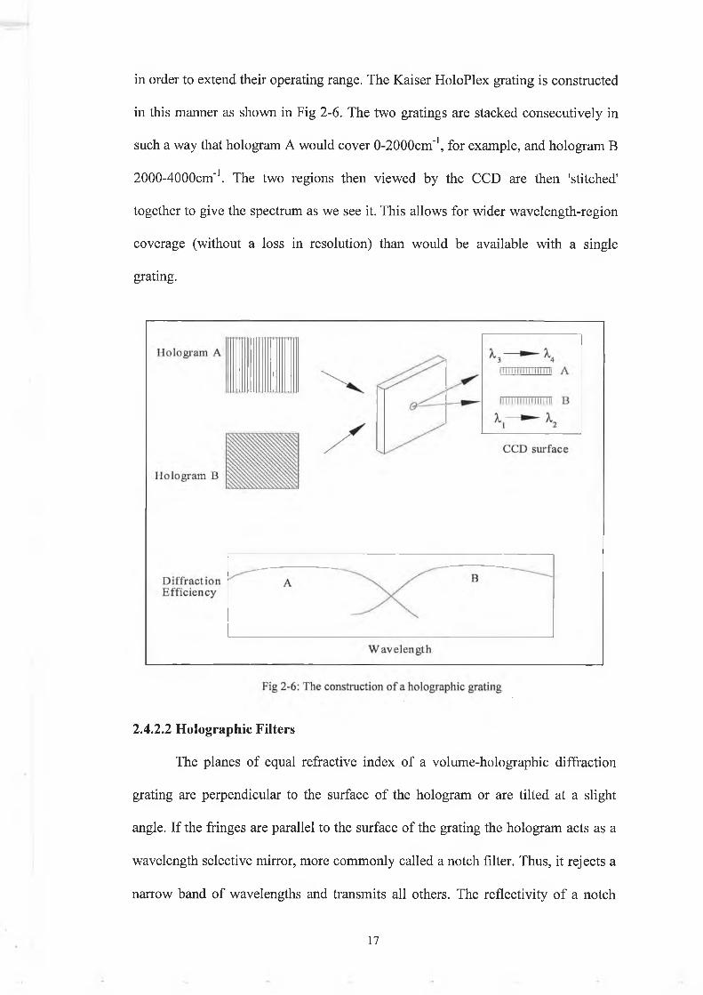
in order to extend their operating range. The Kaiser HoloPlex grating is constructed

in this manner as shown in Fig 2-6. The two gratings are stacked consecutively in

such a way that hologram A would cover 0-2000cm'1, for example, and hologram B

2000-4000cm'1. The two regions then viewed by the CCD are then 'stitched'

together to give the spectrum as we see it. This allows for wider wavelength-region

coverage (without a loss in resolution) than would be available with a single

grating.

2.4.2.2 Holographic Filters

The planes of equal refractive index of a volume-holographic diffraction

grating are perpendicular to the surface of the hologram or are tilted at a slight

angle. If the fringes are parallel to the surface of the grating the hologram acts as a

wavelength selective mirror, more commonly called a notch filter. Thus, it rejects a

narrow band of wavelengths and transmits all others. The reflectivity of a notch

1 7

filter can be quite high and its bandwidth narrow. This makes notch filters ideal

laser light rejection filters for work in Raman spectroscopy. The greatest advantage

of a holographic notch filter is the smoothness of its transmission curve, which

means it performs much better at low wavenumbers than a thin dielectric filter.

Undulations in a dielectric filter's transmission curve means that the measurement

of vibrational frequencies below 400-500cm'1 becomes nearly impossible. Also, the

holographic filter has a narrower rejection band that further enhances its low

frequency performance advantage.

2.4.2.3 The Axial Transmission Spectrograph

The axial transmissive spectrograph for the Holoprobe uses a holographic

transmission grating in combination with well corrected camera lenses to achieve

peak performance. The diffracted light from the spectrograph stage is focused onto

the surface of a CCD detector, which records the actual spectrum. The light path is

axially symmetric through the input and output lenses which minimises aberrations

in the system. The grating is at an angle close to 45° so that the diffracted light is

forced into the +1 order for highest diffraction efficiency. The complete

spectrograph is shown overleaf in Fig. 2-7. The first lens collimates the input signal

from the slit, which then passes through the notch filter to attenuate the laser light.

The filtered signal is incident on the grating and focused onto the CCD by the

second lens. The slit also functions as a resolution spatial filter to minimise the

transmission of stray light into the dispersion stage of the spectrograph.

18

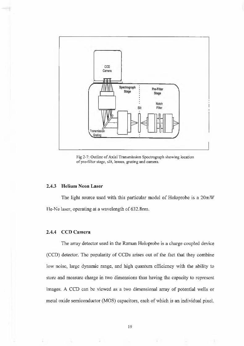
Fig 2-7: Outline o f Axial Transmission Spectrograph showing location o f pre-filter stage, slit, lenses, grating and camera.

2.4.3 Helium Neon Laser

The light source used with this particular model of Holoprobe is a 20mW

He-Ne laser, operating at a wavelength of 632.8nm.

2.4.4 CCD Camera

The array detector used in the Raman Holoprobe is a charge coupled device

(CCD) detector. The popularity of CCDs arises out of the fact that they combine

low noise, large dynamic range, and high quantum efficiency with the ability to

store and measure charge in two dimensions thus having the capacity to represent

images. A CCD can be viewed as a two dimensional array of potential wells or

metal oxide semiconductor (MOS) capacitors, each of which is an individual pixel.

1 9

The number of electrons collected in a well is directly proportional to the number of

photons incident on that pixel. The best signal to noise ratio is obtained when the

exposure of the CCD detector allows the wells to nearly fill. The most significant

source of noise in most CCDs is quantum or 'shot' noise. Shot noise arises from the

random arrival times and energies of incident photons. Two consecutive spectral

measurements of the same sample will always show some variation in the number

of photons collected at any pixel. Longer collection times can reduce the relative

levels of shot noise.

Dark current and cosmic rays can also contribute to the production of

inaccurate spectra. Dark current is a background external current that is produced

even when there is no radiation incident on the detector and leads to a dark current

curve. Cosmic rays are high-energy particles, originating from space that lead to

spikes in the spectra. The contributions from both dark current and cosmic rays can

be corrected for within the software package.

2.4.5 Fibre Optic Probe

Multimode optical fibres are an excellent choice for laser light delivery and

collection. They are small, can be used for remote or laboratory sampling and

provide stable reproducible signals from solids, liquids and gases. However silica

optical fibres themselves are a source of considerable background signal. As the

laser light is travelling down a length of fibre, it generates an intense silica Raman

spectrum. Fluorescence from the fibre cladding and from the cement holding the

bundle together is also generated. These signals emerge from the fibre head along

with the laser light. They are then reflected from any solid or liquid and collected

with the Raman spectrum of the sample. This reflected laser light generates more

2 0

background as it returns down the fibre and these signals can obscure weak Raman

signals. The fibre optic probe in the Holoprobe, shown in Fig. 2-8 eliminates this

problem by using a lens to both filter the laser light before fibre delivery onto the

sample and to collimate the Raman scattered light. Also the collected light is

focused onto a single fibre.

The light emerging from the fibre is collimated by lens assembly PL-1 and

passes through a holographic transmission grating, G in Fig. 2-8, which diffracts

the laser light towards a spatial filter (PL2 and PL3). The laser is then focused on

the sample. Only the laser wavelength passes through this spatial filter as all the

silica Raman light is removed at this stage. The collected Raman scatter, along with

the Rayleigh scatter and reflected laser radiation, is passed through a pair of notch

filters. These filters remove reflected laser light and any fibre background generated

as the Raman signal travels to the spectrograph. The use of microscope objective

lenses, PL4, allows efficient delivery and collection with single fibres. The Raman

signal is then focused onto the fibre by PL5

Fig 2-8: Diagram o f fibre optic probe-head design showing lenses one through five (PL1-PL5), power adjustment control (PA), grating (G), diffuse screen indicator (DS), probe head shutter, spatial filter (SF), beam combiner and notch filters, and the linear polarisers (PB).

2 1

The de facto industry standard ratio for the ammonium/peroxide mixture

(APM) is a 1:1:5 ratio of H202:NH40H:H20 . Therefore the samples used in this

study were made up in this way. Some results were also obtained for 1:1:4 and

1:1:6 ratios as well. For the 1:1:5 mix, 300ml of de-ionised water was used.

Without dilution the NH4OH and H2O2 were described as being 100% solutions for

this particular example. The NH4OH and H2O2 were kept at a constant volume of

50ml. The ammonia and peroxide were ratioed inversely in such a way that their

sum total equalled 100%. For example, if there was 30ml of peroxide, this meant

that 20ml of ammonia was present, i.e. 60% peroxide and 40% ammonia. To obtain

these percentages the peroxide and ammonia were diluted. Therefore a 50 %

ammonia solution was obtained by adding 25ml of water to 25ml of ammonia.

Spectra were taken at 5% increments, as detailed overleaf.

Samples were prepared as required. For each change in percentage peroxide

and ammonia, new solutions were made up. The SC-1 was not allowed to stand for

any time and spectra were taken almost immediately. Also for each percentage data

point, three batches of that concentration were prepared and analysed.

2.5 Sam ple Preparation

% Peroxide % Ammonia ml Peroxide ml Ammonia ml Water

0 100 0.0 50.0 300

5 95 2.5 47.5 300

10 90 5.0 45.0 300

15 85 7.5 42.5 300

20 80 10.0 40.0 300

25 75 12.5 37.5 300

2 2

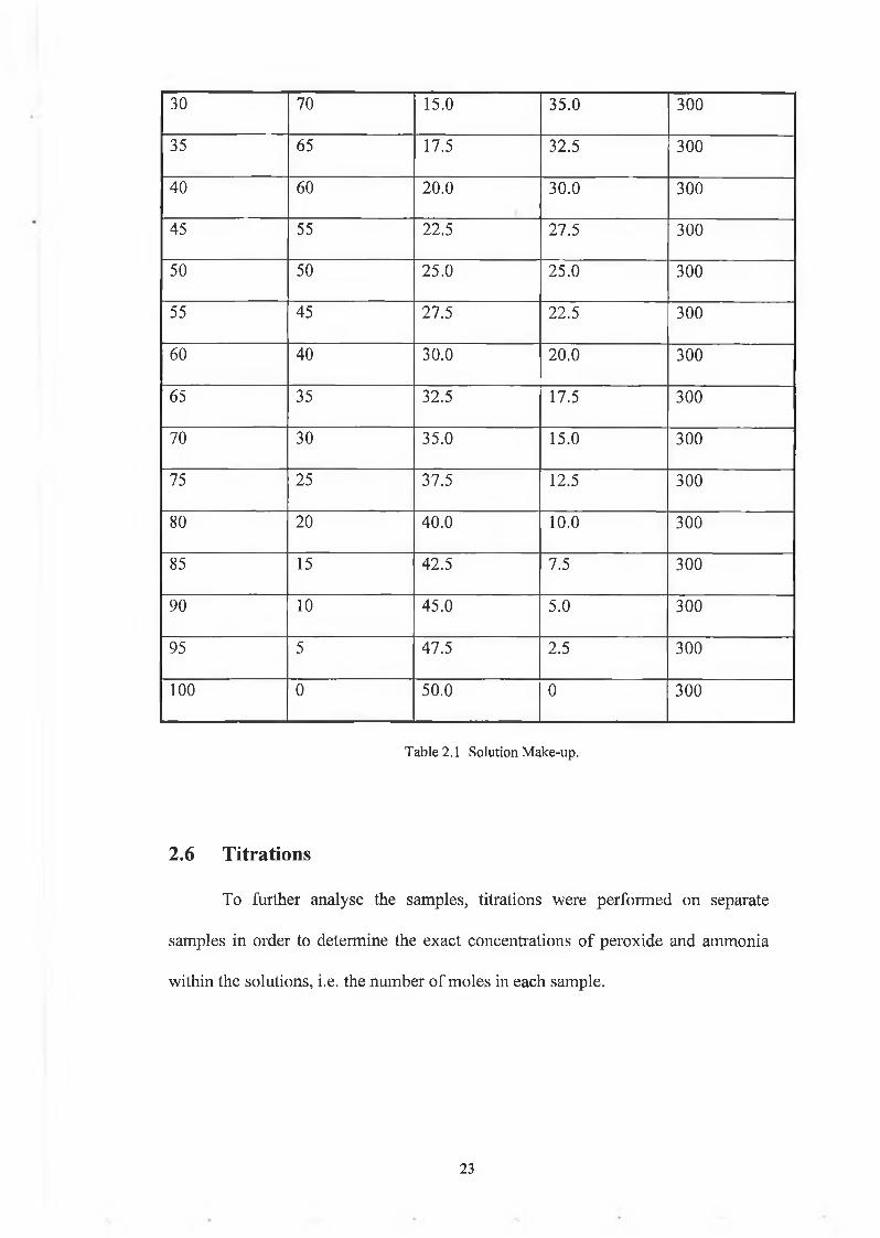
30 70 15.0 35.0 300

35 65 17.5 32.5 300

40 60 20.0 30.0 300

45 55 22.5 27.5 300

50 50 25.0 25.0 300

55 45 27.5 22.5 300

60 40 30.0 20.0 300

65 35 32.5 17.5 300

70 30 35.0 15.0 300

75 25 37.5 12.5 300

80 20 40.0 10.0 300

85 15 42.5 7.5 300

90 10 45.0 5.0 300

95 5 47.5 2.5 300

100 0 50.0 0 300

Table 2.1 Solution Make-up.

2.6 Titrations

To further analyse the samples, titrations were performed on separate

samples in order to determine the exact concentrations of peroxide and ammonia

within the solutions, i.e. the number of moles in each sample.

2 3

2.6.1 Hydrogen Peroxide

Potassium permanganate is a powerful oxidising agent and can be used to

estimate the end-point of titrations involving reducing agents such as H2O2. 5ml

samples of SC-1 were taken and the appropriate amount of sulphuric acid added in

order to facilitate the reaction. No indicator is needed for permanganate titrations.

5H 20 2 + 2KMnOA + 3H 2S 0 4 -> K2SOA + 2MnSOA + 8H 20 + 50 2 (2.12)

2.6.2 Ammonium Hydroxide

The first approach to titrating the ammonia was to employ a back titration

method using sulphuric acid (H2SO4) and sodium hydroxide (NaOH). 5ml samples

of SC-1 were taken from the batch solution and excess sulphuric acid was added to

this. The sulphuric acid served to neutralise any ammonia in the solution and the

excess was then titrated with NaOH using a phenolphthalein indicator. By

calculating how much excess H2SO4 was present and how much there was initially,

it was possible to determine how much was used up neutralising the ammonia.

Hence the ammonia concentration was calculated. The reaction processes are

outlined below.

2NHAOH + H 2SOA ->(NH4)2S 0 A+2H20 (2.13)

2NaOH + H 2SOa -> Na2S 0 A+2H20 (2.14)

This titration method proved unreliable over time, possibly due to the fact that

NaOH is not a primary standard1. NaOH absorbs CO2 from the atmosphere every

time it is left exposed. This was replaced by sodium carbonate (Na2C03) which is a

primary standard and the H2SO4 was replaced by HC1 simply because it reacts in a

1:1 ratio withNH^OH. The appropriate reactions are:

1 A primary standard is a substance that is easy to obtain, purify, dry and preserve in a pure state

2 4

NH4OH + HCl -> n h 4ci + h 2o

Na2C03 + 2HCl -> 2NaCl + H 20 + C02

(2.15)

(2.16)

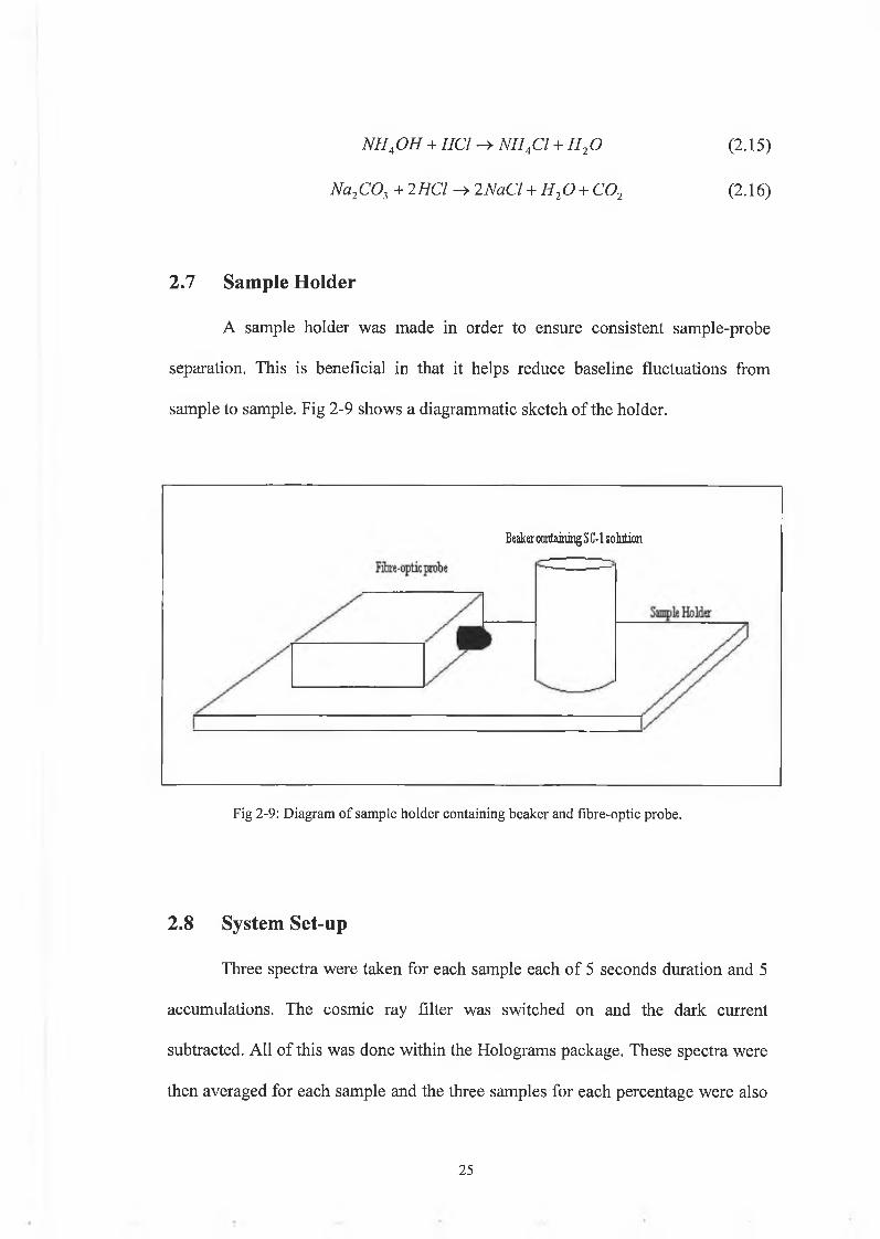
2.7 Sam ple H older

A sample holder was made in order to ensure consistent sample-probe

separation. This is beneficial in that it helps reduce baseline fluctuations from

sample to sample. Fig 2-9 shows a diagrammatic sketch of the holder.

Beaker containing S C-1 solution

Fig 2-9: Diagram o f sample holder containing beaker and fibre-optic probe.

2.8 System Set-up

Three spectra were taken for each sample each of 5 seconds duration and 5

accumulations. The cosmic ray filter was switched on and the dark current

subtracted. All of this was done within the Holograms package. These spectra were

then averaged for each sample and the three samples for each percentage were also

2 5

averaged to one. The spectra were then exported to the chemoraetrics software

package, Unscrambler 7.01, where all of the analyses were performed

2 6

Chapter 3

Chemometrics

3.1 Introduction

Multivariate analysis, or chemometrics as it is widely known, has been

defined as the chemical discipline that uses mathematical, statistical and other

methods employing formal logic to (a) design or select optimal measurement

procedures and experiments, and (b) provide maximum relevant chemical

information by analysing chemical data.1351 The advantage of multivariate

techniques as opposed to, say, the univariate approach is that by taking into account

every, or at least a large number of variables from a spectrum, it is possible to

gauge the influence of each particular data point on a model. This contrasts with the

univariate approach where discarding potentially valuable information is possible.

Multivariate calibration, then, means determining how to use many measured

variables xi, *2,.............. xn simultaneously for quantifying some target variable y P 6]>

In this work the Raman signal at various wavelengths and the concentration of the

peroxide/ammonia are the x and y variables respectively.

3.2 Univariate Analysis

Univariate analysis is best described as simple linear regression, i.e. where

there is one y variable being predicted from a second one, x, e.g. the intensity at a

single wavelength and the relationship between the two is linear. In other words all

observations are dependent upon a single variable x.

2 7

Least-Squares regression is used to describe the relationship between y and

x in general. The following method is as outlined in the work of Tedesco e t alP4]

This relationship can be defined by the function y=f{x,a,b\ ,b„) where

a,bi........ bm are constant coefficients characteristic of the regression line,

representing the intercept of the line with the y-axis and the gradient of the line,

respectively. The x value is the controlled or independent variable whereas the y

value is the dependent or measured variable. This means that there is assumed to be

no error in the x variable. However, on the condition that the error in preparing the

samples is significantly smaller than the measurement error, which is usually the

case, then this is a safe assumption for calibration problems. The values of a and b

must be chosen so as to best fit the experimental data (x\, y\). If the relationship

between x and y is considered to be a straight line then the relationship between

each observation pair (xj, y\) can be described as

y i =a + bxi (3.1)

with the values of y being the estimated, model values. The generally accepted

requirements for deriving the best straight line between x and y is that the

difference between the measured and fitted line is minimised. The most popular

technique to minimise this error is the least squares method. For each measured

value the deviation between the derived model value and the measured data is given

by yi ~ y, • The total error between the model and the observed data is the sum of

these individual errors. Each error is squared to make each value positive.

Therefore, the total error, e, is

s = Y jo > -y ^ f (3-2)1=1

3.2.1 Least Squares Regression

2 8

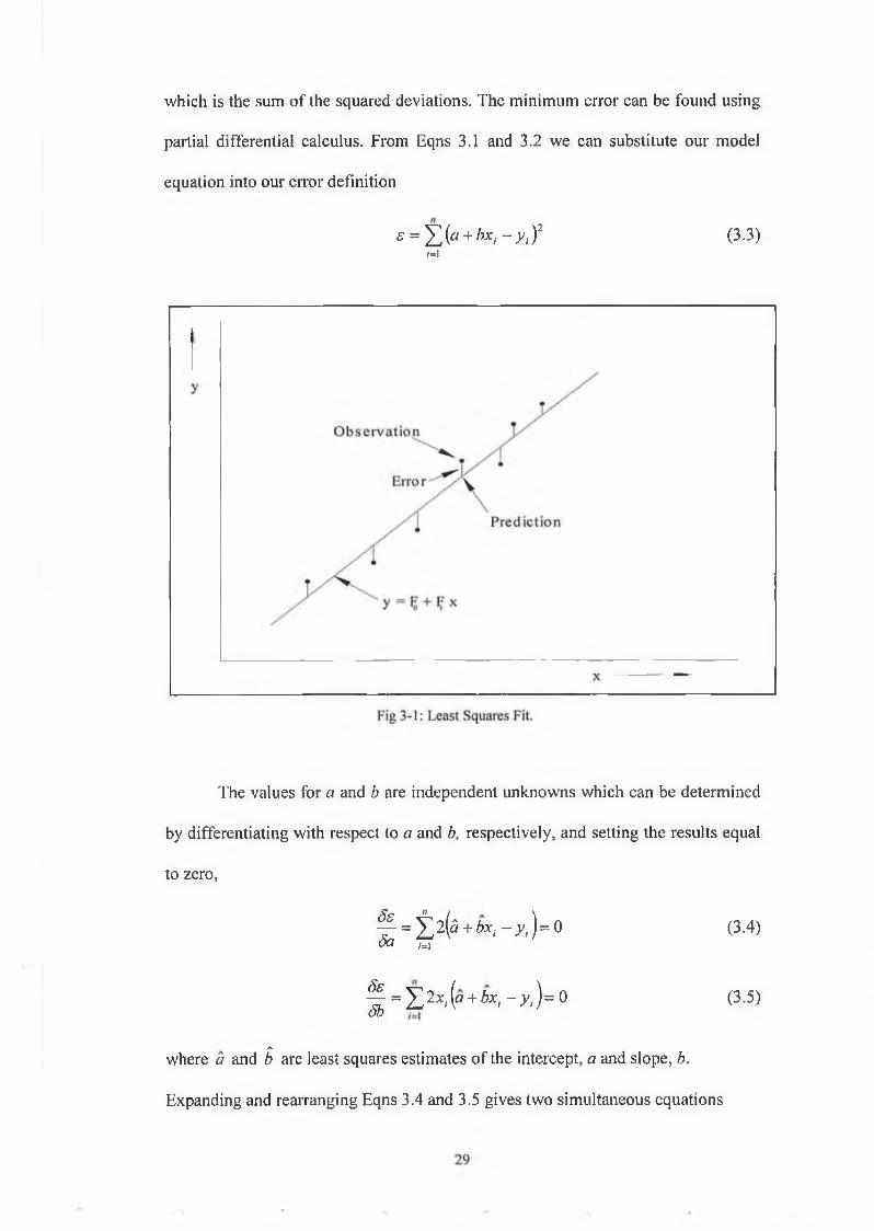
which is the sum of the squared deviations. The minimum error can be found using

partial differential calculus. From Eqns 3.1 and 3.2 we can substitute our model

equation into our error definition

s = Y J(a + bxi - y , ) 2 (3.3)M

The values for a and b are independent unknowns which can be determined

by differentiating with respect to a and b, respectively, and setting the results equal

to zero,

^ = ¿ 2 ( 5 + 6^ - x ) = 0 (3.4)5a t i

^ = Y p .x i{a + b x , - y ) = 0 (3.5)

Awhere a and b are least squares estimates of the intercept, a and slope, b.

Expanding and rearranging Eqns 3.4 and 3.5 gives two simultaneous equations

(3 .6)

(3.7)

from which the following expressions can be derived,

(3.8)

and

¿ = £ ( y'- * X y t - y )

E f e - * ) 2(3.9)

where x and y represent the mean values of x and y.

3.3 M ultivariate Analysis: An Exam ple

Univariate analysis is limited to modelling a dependent variable with a

single independent variable. However chemometrics is more often concerned with

multivariate measurements. Therefore it is important to extend our understanding of

regression to include eases in which several independent variables contribute to the

measured response. 34]

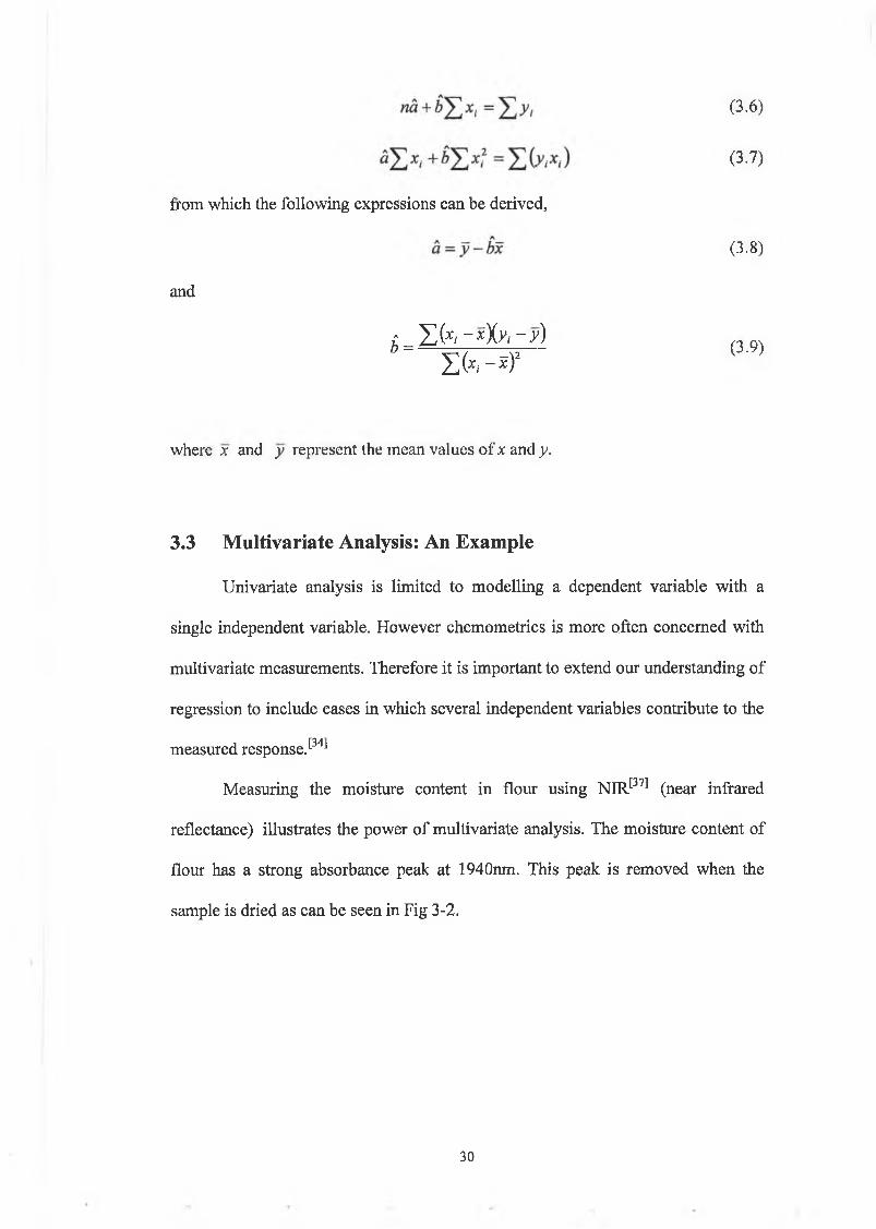
Measuring the moisture content in flour using NIR[37] (near infrared

reflectance) illustrates the power of multivariate analysis. The moisture content of

flour has a strong absorbance peak at 1940nm. This peak is removed when the

sample is dried as can be seen in Fig 3-2.

3 0

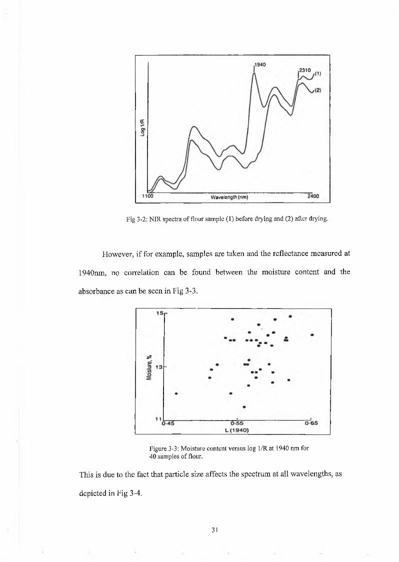
Fig 3-2: NIR spectra of flour sample (1) before drying and (2) after drying.

However, if for example, samples are taken and the reflectance measured at

1940nm, no correlation can be found between the moisture content and the

absorbance as can be seen in Fig 3-3.

Figure 3-3: Moisture content versus log 1/R at 1940 nm for 40 samples o f flour.

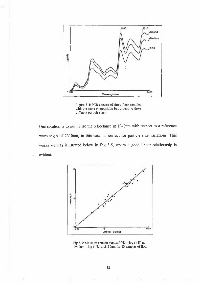
This is due to the fact that particle size affects the spectrum at all wavelengths, as

depicted in Fig 3-4.

3 1

Wavelength (nm)

Figure 3-4: NIR spectra o f three flour samples with the same composition but ground to three different particle sizes.

One solution is to normalise the reflectance at 1940nm with respect to a reference

wavelength of 2310nm, in this case, to correct for particle size variations. This

works well as illustrated below in Fig 3-5, where a good linear relationship is

evident.

Fig 3-5: Moisture content versus AOD = log (1/R) at 1940nm - log (1/R) at 2130nm for 40 samples o f flour.

3 2

The preceding example perfectly illustrates the need in some cases for

multiple wavelength selection.

3.3.1 Introduction to Multivariate Analysis

In its simplest form, the dependent response variable, y, may be a function

of two such independent variables, x\ and Xi.

y = a + bxxx +b2x2 (3.10)

Here a is the intercept on the ordinate y-axis, and b\ and bj are the partial regression

coefficients. These coefficients denote the rate of change of the mean of y as a

function of xi, with X2 constant, and the rate of change of y as a function of X2 with

x\ constant respectively. The statistical technique most commonly used to derive a

and b\ bm is Multiple Linear Regression (MLR). It is however becoming

popular to use Principal Components Regression (PCR) and Partial Least Squares

Regression (PLS). The methodology used here to derive an understanding of these

techniques is a rather intuitive one. Details of the precise algorithms for principal

components analysis and partial least squares regression may be found in the

appendices. Two concepts needed in order to understand these techniques are (a)

fitting a line by least squares, which was dealt with in the previous section and (b)

the projection of a multi-dimensional cloud of data points onto a line, which can be

visualised quite easily. By combining these two techniques it is possible to gain an

insight into MLR, PCR and PLS.[37]

From the method of least squares we have the equation^ = a+bix. If a and

b are found from the plot by measuring the intercept (a) and the slope (¿1), y can be

predicted from x using the equation and the plot can be discarded. It is common,

however that more than one x is needed for predicting y, i.e. in the case of

3 3

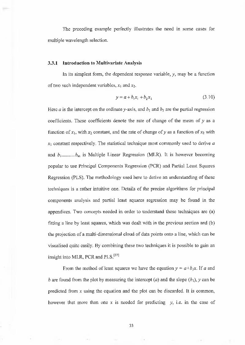
overlapping peaks. This means that we have at least two spectral measurements or

two x's, X) and xi. By ignoring y, temporarily, X2 can be plotted against x\ for the

calibration samples as in Fig 3-6(a) below. The data are displayed as a point cloud

in two dimensions. With one x only one dimension is needed to represent the point

cloud as in Fig 3-6(b). If we had data as in Fig 3-6(b) it would be possible to find an

equation using least squares.

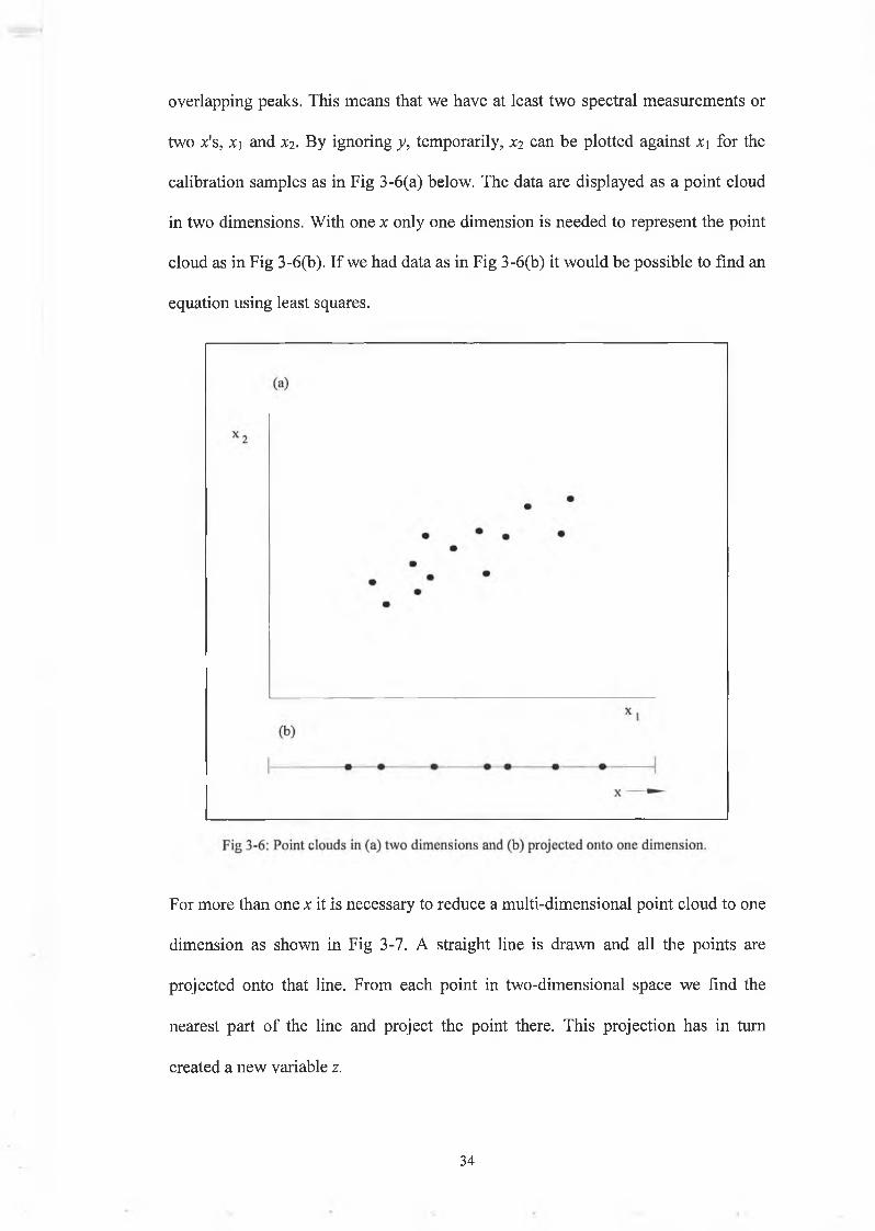
For more than one x it is necessary to reduce a multi-dimensional point cloud to one

dimension as shown in Fig 3-7. A straight line is drawn and all the points are

projected onto that line. From each point in two-dimensional space we find the

nearest part of the line and project the point there. This projection has in turn

created a new variable z.

3 4

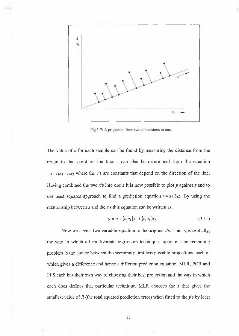
The value of z for each sample can be found by measuring the distance from the

origin to that point on the line, z can also be determined from the equation

z=ciX\+C2X2 where the c's are constants that depend on the direction of the line.

Having combined the two x's into one z it is now possible to plot y against z and to

use least squares approach to find a prediction equation y=a+b\z. By using the

relationship between z and the x's this equation can be written as.

y = a + (b]c1)xl + {bxc2)x2 (3.11)

Now we have a two variable equation in the original x's. This is, essentially,

the way in which all multivariate regression techniques operate. The remaining

problem is the choice between the seemingly limitless possible projections, each of

which gives a different z and hence a different prediction equation. MLR, PCR and

PLS each has their own way of choosing their best projection and the way in which

each does defines that particular technique. MLR chooses the z that gives the

smallest value of R (the total squared prediction error) when fitted to the / s by least

3 5

squares. PCR and PLS in their simplest form operate in the same way as MLR, i.e.

create a z by projection and predict y from z by least squares.

PCR chooses its projection without looking at the ys. It chooses so that z

has as much variability as possible in order to create the best one-dimensional

picture of the original x's. PLS combines both methods by choosing a projection

that balances the variability of z and the error in predicting the known ys. In other

words, it maximises the variability of z times the squared correlation of the y-z

equation. Clearly the mathematics generalises to more variables as can be seen

from the algorithms in appendices A and B, and in practice, formulae are used to

find a and b directly. However this intuitive method, as described in the Near Infra-

Red Publications (NIRP) chemometrics training course|37], gives an excellent

insight into the principles of multivariate regression.

3.3.2 Principal Components Analysis

To gain further insight into multivariate analysis it is useful to examine

Principal components Analysis (PCA) in more detail. PCA forms the basis for the

regression techniques used in this work and also it provides an excellent foundation

for the understanding of PLS and PCR.

PCA is a data compression technique that can reduce a large number of

variables into small number of new uncorrected variables, which retain most of the

information of the original set.[3S| PCA is widely applicable to e.g. interpreting the

chemical influence of specific components without prior knowledge of the chemical

composition of the samples. It can also be used for identifying the influence of

instrumentation on the data collected and how this can be used to improve

instrument design.

3 6

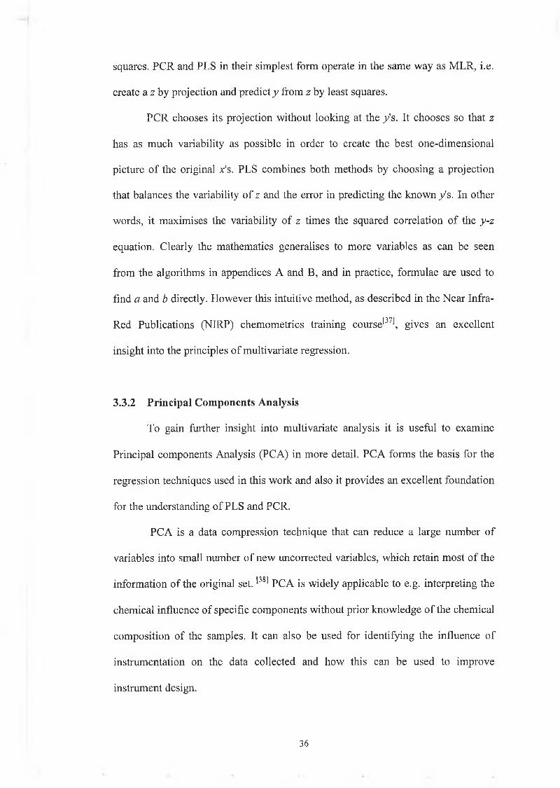
PC A can be interpreted in terms of a 3-D data cloud. Although the number

of dimensions in reality is much higher it gives a useful insight into the workings of

PCA. The first step is to centre the data. This moves the origin from the bottom left

comer to the centre of our space. The principal components are the new axes on

which we will plot the data. The derivation of principal components (PC) are

governed by the following rules:

• All PC’s must pass through the origin

• PC's are orthogonal variables, i.e. they lie at right angles to each

other

• PC's are derived in fixed sequence, with each PC representing

less variation than the previous PC.

The first PC is the line, passing through the origin, which represents the

maximum variation in the data. This maximum variation can be determined by least

squares

3.3.2.1 Geometric Interpretation o f Principal Components Analysis

Fig 3-8:Projcction o f data cloud onto its principal components.

3 7

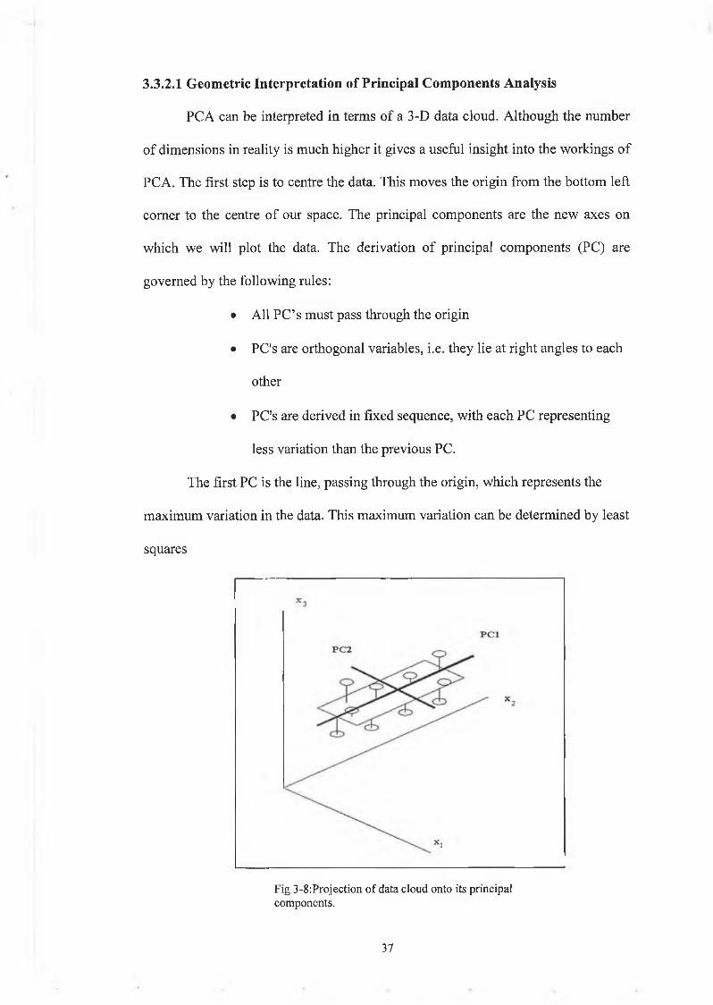
Two variables that define the first PC can be calculated now that its position

is fixed. PC loadings are the rotations required to move the original axes to the

position of the new PC. They are in fact the cosines of the angles between the new

and each original variable.

Fig 3-9: Determination o f PC loadings.

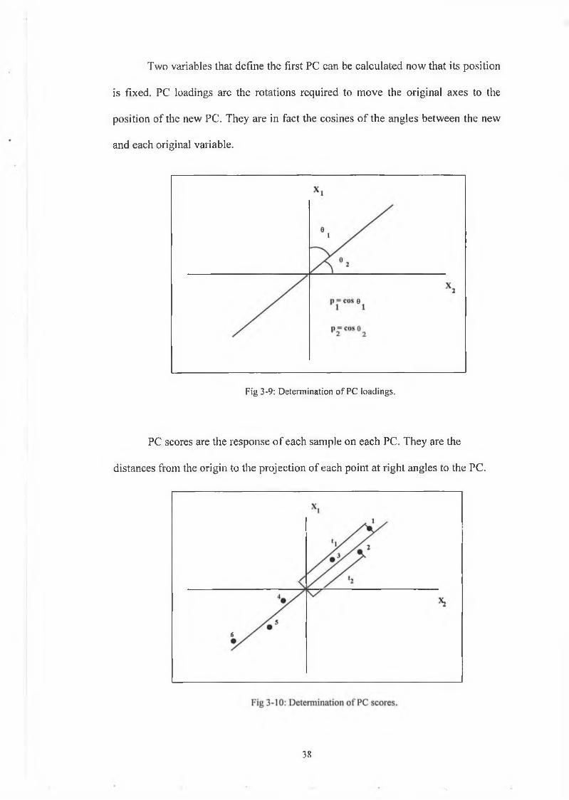
PC scores are the response of each sample on each PC. They are the

distances from the origin to the projection of each point at right angles to the PC.

3 8

Chapter 4

Data Analysis

4.1 Introduction

The data collection and analysis was carried out in a stepwise fashion in

which there were three main procedures.

1. Firstly, a simple univariate analysis was carried out in order to establish

the basis for the technique, i.e. an experimental set of data to prove that

the hydrogen peroxide and ammonium hydroxide peaks vary linearly

with concentration.

2. Secondly, a multivariate calibration and validation were carried out, of

which there were two parts. A simple percentage method was first

performed to prove the efficacy of the multivariate approach, followed

by a more absolute determination of concentrations, the results of which

were verified by titrations.

3. Finally, a second multivariate calibration and validation was performed

in an attempt to further improve the accuracy of predictions and thus

reduce the error.

4 0

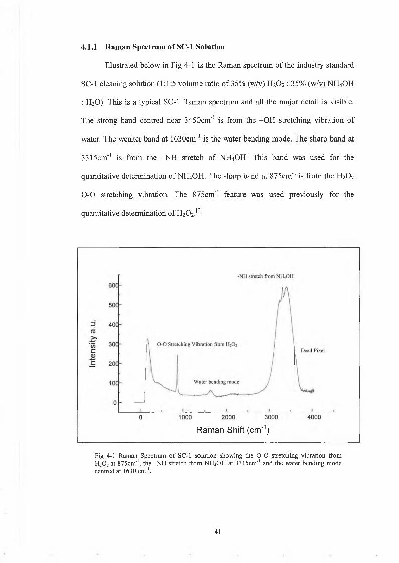
Illustrated below in Fig 4-1 is the Raman spectrum of the industry standard

SC-1 cleaning solution (1:1:5 volume ratio of 35% (w/v) H2O2 : 35% (w/v) NH4OH

: H2O). This is a typical SC-1 Raman spectrum and all the major detail is visible.

The strong band centred near 3450cm'1 is from the -OH stretching vibration of

water. The weaker band at 1630cm"1 is the water bending mode. The sharp band at

3315cm'1 is from the -NH stretch of NH4OH. This band was used for the

quantitative determination of NH4OH. The sharp band at 875cm'1 is from the H2O2

0 -0 stretching vibration. The 875cm'1 feature was used previously for the

quantitative determination of H202.[3]

4.1.1 Raman Spectrum of SC-1 Solution

Raman Shift (cm'1)

Fig 4-1 Raman Spectrum o f SC-1 solution showing the 0 - 0 stretching vibration from H20 2 at 875cm'1, the -N H stretch from NH4OH at 3315cm'1 and the water bending mode centred at 1630 cm-1.

4 1

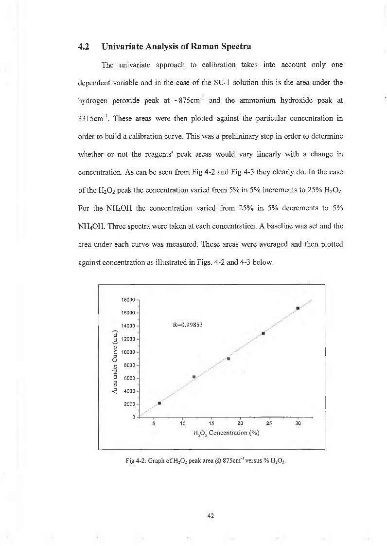
The univariate approach to calibration takes into account only one

dependent variable and in the case of the SC-1 solution this is the area under the

hydrogen peroxide peak at ~875cm'1 and the ammonium hydroxide peak at

3315cm'1. These areas were then plotted against the particular concentration in

order to build a calibration curve. This was a preliminary step in order to determine

whether or not the reagents' peak areas would vary linearly with a change in

concentration. As can be seen from Fig 4-2 and Fig 4-3 they clearly do. In the case

of the H2O2 peak the concentration varied from 5% in 5% increments to 25% H2O2.

For the NH4OH the concentration varied from 25% in 5% decrements to 5%

NH4OH. Three spectra were taken at each concentration. A baseline was set and the

area under each curve was measured. These areas were averaged and then plotted

against concentration as illustrated in Figs. 4-2 and 4-3 below.

4.2 Univariate A nalysis o f Ram an Spectra

18000

16000

14000

12000<Dt 100003of t 8000 'Tj3 6000cs(D

-5 4000

2000

0

R=0.99853

— 1 1 * 1 * 1-----1-----1-10 15 20 25 30

H 20 2 Concentration (%)

Fig 4-2: Graph o f H20 2 peak area @ 875cm"1 versus % H20 2.

4 2

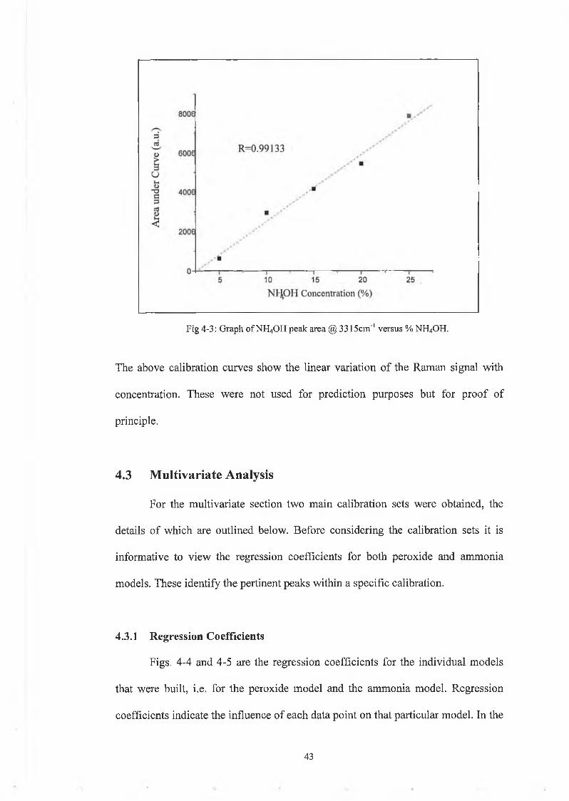
Fig 4-3: Graph o f NH4OH peak area @ 3315cm '1 versus % NH4OH.

The above calibration curves show the linear variation of the Raman signal with

concentration. These were not used for prediction purposes but for proof of

principle.

4.3 M ultivariate Analysis

For the multivariate section two main calibration sets were obtained, the

details of which are outlined below. Before considering the calibration sets it is

informative to view the regression coefficients for both peroxide and ammonia

models. These identify the pertinent peaks within a specific calibration.

4.3.1 Regression Coefficients

Figs. 4-4 and 4-5 are the regression coefficients for the individual models

that were built, i.e. for the peroxide model and the ammonia model. Regression

coefficients indicate the influence of each data point on that particular model. In the

4 3

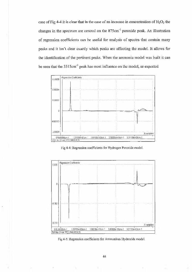
case of Fig 4-4 it is clear that in the case of an increase in concentration of H2O2 the

changes in the spectrum are centred on the 875cm'1 peroxide peak. An illustration

of regression coefficients can be useful for analysis of spectra that contain many

peaks and it isn’t clear exactly which peaks are affecting the model. It allows for

the identification of the pertinent peaks. When the ammonia model was built it can

be seen that the 3315cm'1 peak has most influence on the model, as expected

0D0006-Regression Coefficients

0 00004-

0 00002-

0-

-0 00002-

J V -

............... i ........................... ; ............................. : ]

-000004-X-i/enables

579.00000cm-1 1.23700e+03cm-1 1 B9500e+D3cm-1 2.55300e+03cm-1 3-21100e+03cm-1res114h. (Y-var PC): (MH202.1)

Fig 4-4: Regression coefficients for Hydrogen Peroxide model.

0.005-

0 005

- 0 0 1 0

Regressuin Coefficients

YT

X-variables■------------- i--------------i--------------1-------------- i------579 00000cm-1 1 23700e+03cm-1 1 89500e+03cm-1 2 55300e+03cm-1 3 21100e+C3cm-1

%1143.(Y-var, PC): (%NH4QH.2)

Fig 4-5: Regression coefficients for Ammonium Hydroxide model.

4 4

The primary aim within this calibration set was to acquire a two-

dimensional calibration model by not only varying the H2O2/NH4OH ratio but also

by changing the water ratio. Therefore three sets were measured starting at a 1:1:4

ratio of H2O2: NH4OH : H2O and working up to a 1:1:6 ratio. Within each of these

sets the H2O2/NH4OH ratio was varied from 0% H202/100% NH4OH in 5%

increments/decrements to 100% H2C>2/0% NH4OH. Three samples were made up

for each step and three spectra were recorded for each sample. To obtain an

absolute measurement three 5mL samples were titrated to obtain the number of

moles of both peroxide and ammonia as outlined in section 4.2. Therefore both

percentage and molar calibration sets were obtained for each ratio.

4.3.2.1 Percentage Models, Hydrogen Peroxide

Shown below in Fig 4-6 is the scores plot for the 1:1:5 percentage models

for both peroxide and ammonia. As illustrated in Chapter 3, scores are the response

of each sample on each principal component (PC). Therefore, it is useful to look at

the scores plot for the detection of outliers. For each model built the accompanying

scores plot is shown.

4.3.2 Calibration 1

PC2 Scores

-1500 -1000 -500 0 500 1000 1500% 1l5h.X-expl 95%.2% Y-expl 99%. 1%

Fig 4-6: Scores plot for H20 2 ‘percentage’ model.

4 5

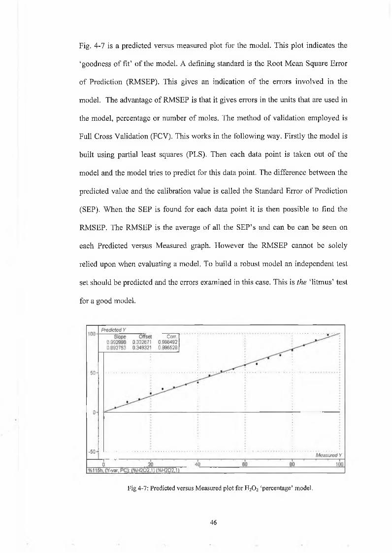
Fig. 4-7 is a predicted versus measured plot for the model. This plot indicates the

‘goodness of fit’ of the model. A defining standard is the Root Mean Square Error

of Prediction (RMSEP). This gives an indication of the errors involved in the

model. The advantage of RMSEP is that it gives errors in the units that are used in

the model, percentage or number of moles. The method of validation employed is

Full Cross Validation (FCV). This works in the following way. Firstly the model is

built using partial least squares (PLS). Then each data point is taken out of the

model and the model tries to predict for this data point. The difference between the

predicted value and the calibration value is called the Standard Error of Prediction

(SEP). When the SEP is found for each data point it is then possible to find the

RMSEP. The RMSEP is the average of all the SEP’s and can be can be seen on

each Predicted versus Measured graph. However the RMSEP cannot be solely

relied upon when evaluating a model. To build a robust model an independent test

set should be predicted and the errors examined in this case. This is the ‘litmus’ test

for a good model.

Fig 4-7: Predicted versus Measured plot for H20 2 ‘percentage’ model.

4 6

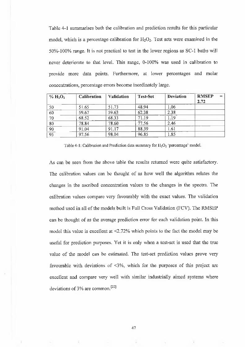
Table 4-1 summarises both the calibration and prediction results for this particular

model, which is a percentage calibration for H2O2. Test sets were examined in the

50%-100% range. It is not practical to test in the lower regions as SC-1 baths will

never deteriorate to that level. This range, 0-100% was used in calibration to

provide more data points. Furthermore, at lower percentages and molar

concentrations, percentage errors become inordinately large.

% h 2o 2 Calibration Validation Test-Set Deviation RMSEP = 2.72

50 51.65 51.73 48 .94 1.0660 59.67 59.63 62.38 2.3870 68.52 68.33 71.19 1.1980 78.84 78.60 77.56 2.4690 91.04 91.17 88.39 1.6195 97.56 98.04 96.85 1.85

Table 4-1: Calibration and Prediction data summary for H20 2 ‘percentage’ model.

As can be seen from the above table the results returned were quite satisfactory.

The calibration values can be thought of as how well the algorithm relates the

changes in the ascribed concentration values to the changes in the spectra. The

calibration values compare very favourably with the exact values. The validation

method used in all of the models built is Full Cross Validation (FCV). The RMSEP

can be thought of as the average prediction error for each validation point. In this

model this value is excellent at <2.72% which points to the fact the model may be

useful for prediction purposes. Yet it is only when a test-set is used that the true

value of the model can be estimated. The test-set prediction values prove very

favourable with deviations of <3%, which for the purposes of this project are

excellent and compare very well with similar industrially aimed systems where

deviations of 3% are common.^

4 7

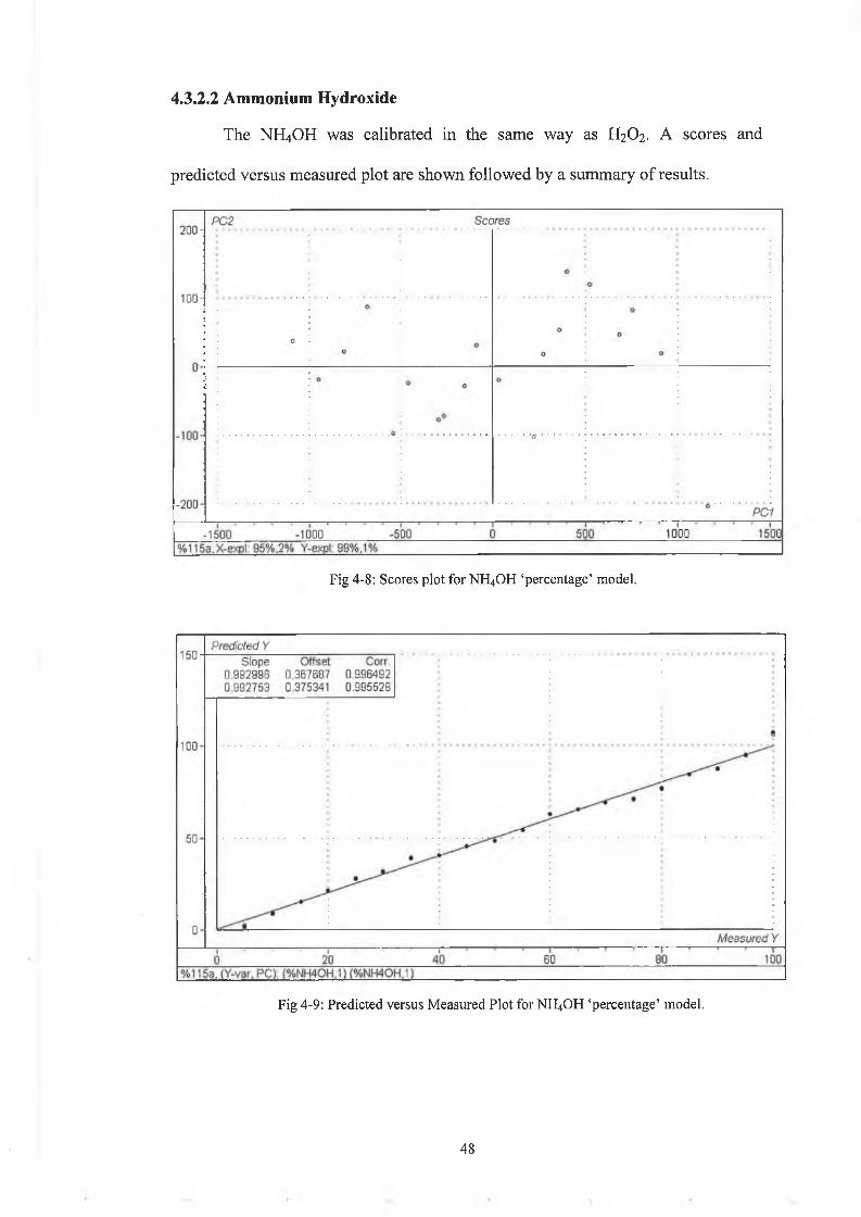
The NH4OH was calibrated in the same way as H2O2. A scores and

predicted versus measured plot are shown followed by a summary of results.

4.3.2.2 Ammonium Hydroxide

Fig 4-8: Scores plot for NH4OH ‘percentage’ model.

Fig 4-9: Predicted versus Measured Plot for NH4OH ‘percentage’ model.

4 8

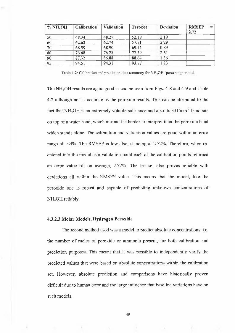
% NH4 0 H Calibration Validation Test-Set Deviation RMSEP = 2.72

50 48.34 48.27 52.19 2.1960 62.62 62.74 57.71 2.2970 68.99 68.90 69.11 0.8980 76.68 76.28 77.39 2.6190 87.32 86.88 88.64 1.3695 94.51 94.31 93.77 1.23

Table 4-2: Calibration and prediction data summary for NH4OH ‘percentage model.

The NH4OH results are again good as can be seen from Figs. 4-8 and 4-9 and Table

4-2 although not as accurate as the peroxide results. This can be attributed to the

fact that NH4OH is an extremely volatile substance and also its 3315cm'1 band sits

on top of a water band, which means it is harder to interpret than the peroxide band

which stands alone. The calibration and validation values are good within an error

range of <4%. The RMSEP is low also, standing at 2.72%. Therefore, when re­

entered into the model as a validation point each of the calibration points returned

an error value of, on average, 2.72%. The test-set also proves reliable with

deviations all within the RMSEP value. This means that the model, like the

peroxide one is robust and capable of predicting unknown concentrations of

NH4OH reliably.

4.3.2.3 Molar Models, Hydrogen Peroxide

The second method used was a model to predict absolute concentrations, i.e.

the number of moles of peroxide or ammonia present, for both calibration and

prediction purposes. This meant that it was possible to independently verify the

predicted values that were based on absolute concentrations within the calibration

set. However, absolute prediction and comparisons have historically proven

difficult due to human error and the large influence that baseline variations have on

such models.

4 9

3 0 0 -P C 2 S e e res

2 0 0 ~

•

•

1 0 0 - 0

0 :O o

• ° •

•

9

* ! o••

- 1 0 0 - •

- 2 0 0 '

e

P C I

1 5 0 0 - 1 0 0 0 - 5 0 0 0 5 0 0 1 0 0 0 1 5 0 0

t r s 1 I 5 h X -e x p l: 9 6 % ,2 % Y -e x p l: 9 9 % ,1 %

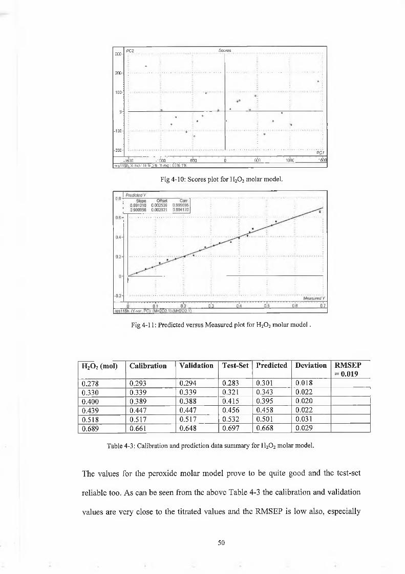
Fig 4-10: Scores plot for H20 2 molar model.

Fig 4-11: Predicted versus Measured plot for H20 2 molar m o d e l.

H20 2 (mol) Calibration Validation Test-Set Predicted Deviation RMSEP = 0.019

0.278 0.293 0.294 0.283 0.301 0.0180.330 0.339 0.339 0.321 0.343 0.0220.400 0.389 0.388 0.415 0.395 0.0200.439 0.447 0.447 0.456 0.458 0.0220.518 0.517 0.517 0.532 0.501 0.0310.689 0.661 0.648 0.697 0.668 0.029

Table 4-3: Calibration and prediction data summary for H20 2 molar model.

The values for the peroxide molar model prove to be quite good and the test-set

reliable too. As can be seen from the above Table 4-3 the calibration and validation

values are very close to the titrated values and the RMSEP is low also, especially

5 0

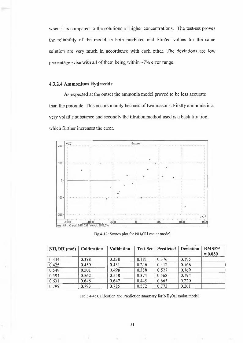
when it is compared to the solutions of higher concentrations. The test-set proves

the reliability of the model as both predicted and titrated values for the same

solution are very much in accordance with each other. The deviations are low

percentage-wise with all of them being within ~7% error range.

4.3.2.4 Ammonium Hydroxide

As expected at the outset the ammonia model proved to be less accurate

than the peroxide. This occurs mainly because of two reasons. Firstly ammonia is a

very volatile substance and secondly the titration method used is a back titration,

which further increases the error.

200 -

10Q-

0-

- 1 0 0 -

1X1

PC2 Scores

o

O

O

*0

O oo

O»0

oo

9

Q

PC1

-1500 -1000 -500 0 500 1000 1500resi 15n.X-exol: 95%.2% Y-expl: 9a% ,0%

Fig 4-12: Scores plot for NH4OH molar model.

NH4OH (mol) Calibration Validation Test-Set Predicted Deviation RMSEP = 0.030

0.334 0.338 0.338 0.181 0.376 0.1950.425 0.450 0.451 0.246 0.412 0.1660.549 0.501 0.498 0.358 0.527 0.1690.591 0.562 0.558 0.374 0.568 0.1940.631 0.646 0.647 0.445 0.665 0.2200.799 0.793 0.785 0.572 0.773 0.201

Table 4-4: Calibration and Prediction summary for NH4OH molar model.

5 1

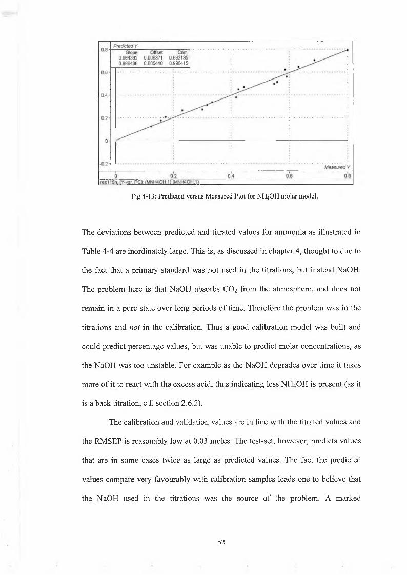
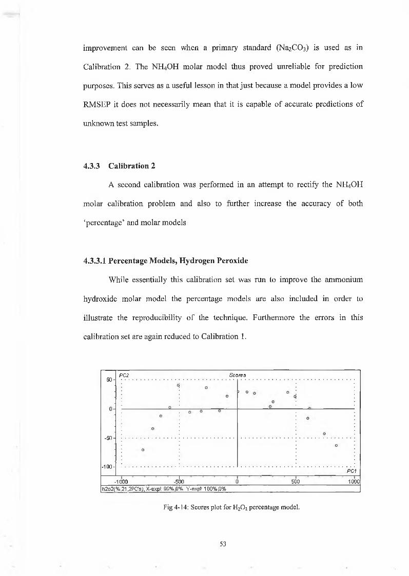
Fig 4-13: Predicted versus Measured Plot for NH4OH molar model.

The deviations between predicted and titrated values for ammonia as illustrated in

Table 4-4 are inordinately large. This is, as discussed in chapter 4, thought to due to

the fact that a primary standard was not used in the titrations, but instead NaOH.

The problem here is that NaOH absorbs CO2 from the atmosphere, and does not

remain in a pure state over long periods of time. Therefore the problem was in the

titrations and not in the calibration. Thus a good calibration model was built and

could predict percentage values, but was unable to predict molar concentrations, as

the NaOH was too unstable. For example as the NaOH degrades over time it takes

more of it to react with the excess acid, thus indicating less NH4OH is present (as it

is a back titration, c.f. section 2 .6.2).

The calibration and validation values are in line with the titrated values and

the RMSEP is reasonably low at 0.03 moles. The test-set, however, predicts values

that are in some cases twice as large as predicted values. The fact the predicted

values compare very favourably with calibration samples leads one to believe that

the NaOH used in the titrations was the source of the problem. A marked

5 2

improvement can be seen when a primary standard (NaiCC^) is used as in

Calibration 2. The NH4OH molar model thus proved unreliable for prediction

purposes. This serves as a useful lesson in that just because a model provides a low

RMSEP it does not necessarily mean that it is capable of accurate predictions of

unknown test samples.

4.3.3 Calibration 2

A second calibration was performed in an attempt to rectify the NH4OH

molar calibration problem and also to further increase the accuracy of both

‘percentage’ and molar models

4.3.3.1 Percentage Models, Hydrogen Peroxide

While essentially this calibration set was run to improve the ammonium

hydroxide molar model the percentage models are also included in order to

illustrate the reproducibility of the technique. Furthermore the errors in this

calibration set are again reduced to Calibration 1.

50-P C 2 Scores

) o

-50 -

-100-

-1000—I—-500 500

PC-I 1000

h2o2(%,21.2PC'S), X-expl 99%.0% Y-expl: 100%,0%

Fig 4-14: Scores plot for H20 2 percentage model.

5 3

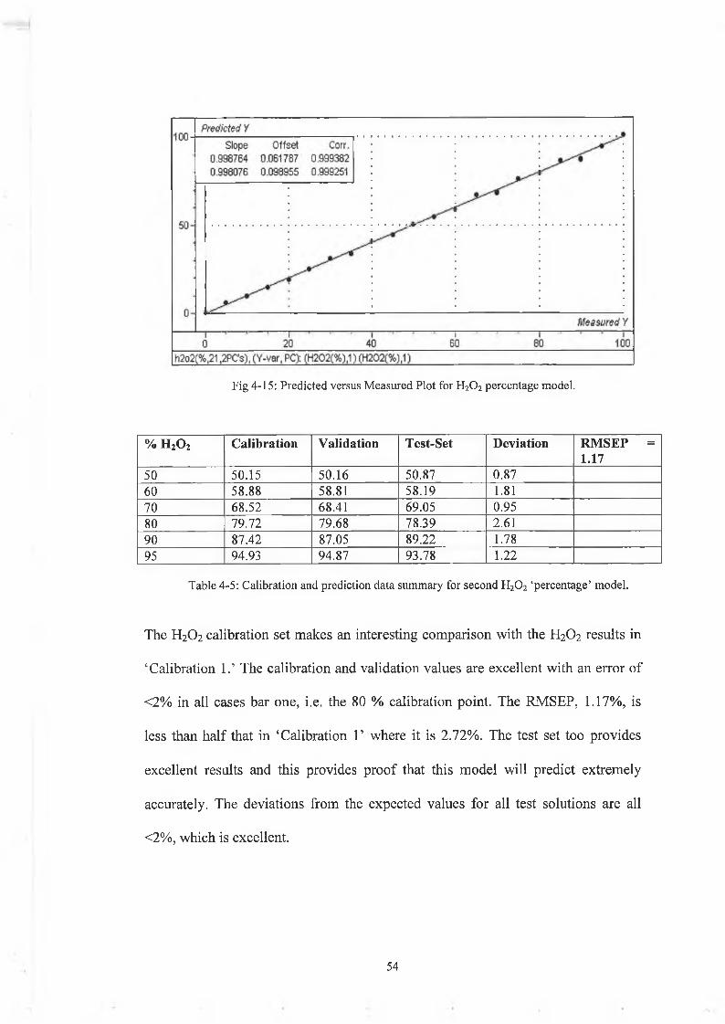
Fig 4-15: Predicted versus Measured Plot for H20 2 percentage model.

% h 2o 2 C a lib ra t io n V a lid a tio n T e s t-S e t D e v ia tio n R M S E P = 1.17

50 50.15 50.16 50.87 0.8760 58.88 58.81 58.19 1.8170 68.52 68.41 69.05 0.9580 79.72 79.68 78.39 2.6190 87.42 87.05 89.22 1.7895 94.93 94.87 93.78 1.22

Table 4-5: Calibration and prediction data summary for second H20 2 ‘percentage’ model.

The H2O2 calibration set makes an interesting comparison with the H2O2 results in

‘Calibration 1.’ The calibration and validation values are excellent with an error of

<2% in all cases bar one, i.e. the 80 % calibration point. The RMSEP, 1.17%, is

less than half that in ‘Calibration 1’ where it is 2.72%. The test set too provides

excellent results and this provides proof that this model will predict extremely

accurately. The deviations from the expected values for all test solutions are all

<2%, which is excellent.

5 4

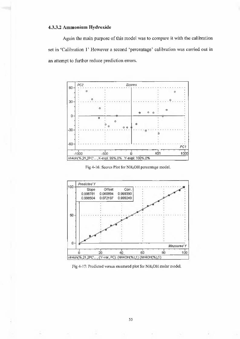
Again the main purpose of this model was to compare it with the calibration

set in ‘Calibration 1’ However a second ‘percentage’ calibration was carried out in

an attempt to further reduce prediction errors.

4.3.3.2 Ammonium Hydroxide

PC2 Scores

0

o

o

o

oO o o

o

oo

P 0o o <

0

p

PC1

- 1000 -500 C 500 1000nh4oh(%.21,2PC... ,X-expl: 99%,0% Y-expl: 100% .0%

Fig 4-16: Scores Plot for NH4OH percentage model.

Fig 4-17: Predicted versus measured plot for NH4OH molar model.

5 5

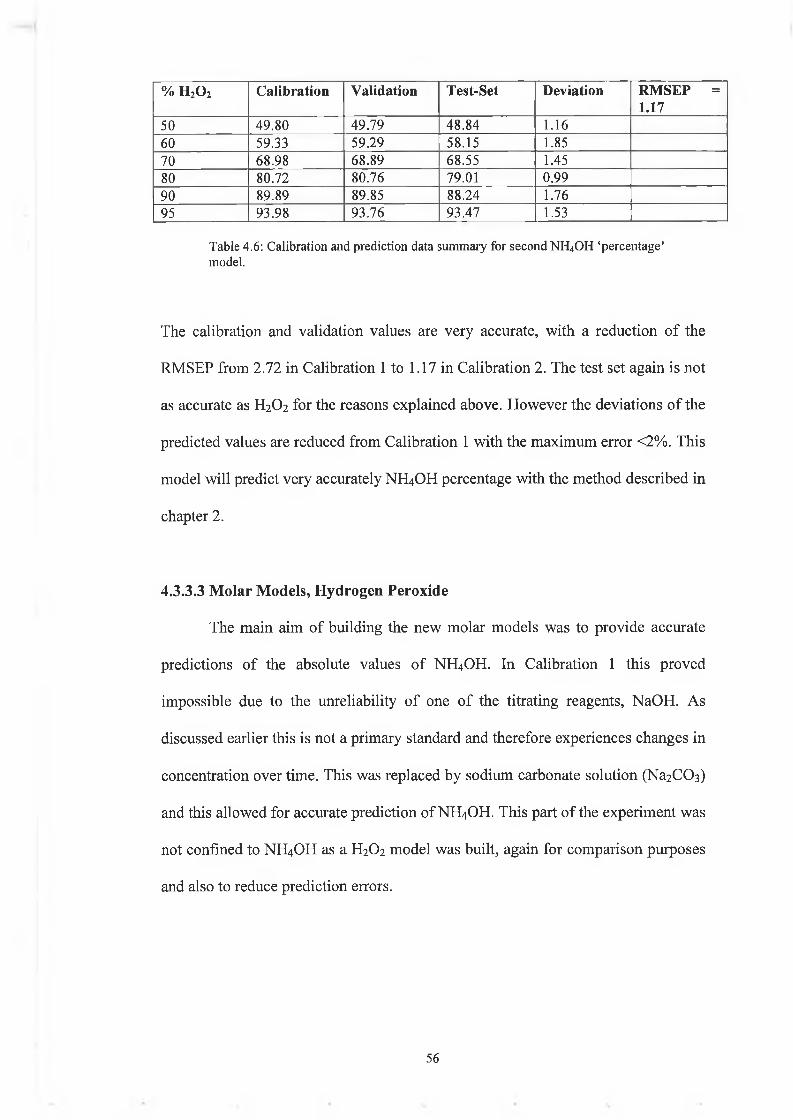
% h 2o 2 C a lib ra t io n V a lid a tio n T e s t-S e t D ev ia tio n R M S E P = 1 .17

50 49.80 49.79 48.84 1.1660 59.33 59.29 58.15 1.8570 68.98 68.89 68.55 1.4580 80.72 80.76 79.01 0.9990 89.89 89.85 88.24 1.7695 93.98 93.76 93.47 1.53

Table 4.6: Calibration and prediction data summary for second NH4OH ‘percentage’model.

The calibration and validation values are very accurate, with a reduction of the

RMSEP from 2.72 in Calibration 1 to 1.17 in Calibration 2. The test set again is not

as accurate as H2O2 for the reasons explained above. However the deviations of the

predicted values are reduced from Calibration 1 with the maximum error <2%. This

model will predict very accurately NH4OH percentage with the method described in

chapter 2 .

4.3.3.3 Molar Models, Hydrogen Peroxide

The main aim of building the new molar models was to provide accurate

predictions of the absolute values of NH4OH. In Calibration 1 this proved

impossible due to the unreliability of one of the titrating reagents, NaOH. As

discussed earlier this is not a primary standard and therefore experiences changes in

concentration over time. This was replaced by sodium carbonate solution (Na2C03)

and this allowed for accurate prediction of NH4OH. This part of the experiment was

not confined to NH4OH as a H2O2 model was built, again for comparison purposes

and also to reduce prediction errors.

5 6

50-P C 2 Scores

; i oo

0o ■

o ° 0* 0

0o

e o

o0

-50-

o0

-100-P C 1

1000 -500 50Q 1000h2o2fmol.20). X-exr)l 9E)%,0% Y-exnl: 10014.0%

Fig 4-18: Scores plot for H20 2 molar model.

Fig 4-19: Predicted versus plot for H20 2 molar model.

H20 2 (mol) Calibration Validation Test-Set Predicted Deviation RMSEP = 0.008

0.260 0.263 0.263 0.263 0.259 0.0040.312 0.307 0.307 0.298 0.284 0.0140.362 0.356 0.355 0.342 0.351 0.0090.417 0.413 0.412 0.398 0.406 0.0080.459 0.452 0.450 0.439 0.454 0.0150.481 0.489 0.491 0.486 0.478 0.008

Table 4-7: Calibration and prediction data summary for second H20 2 molar model.

57

As evidenced by Table 4-7 this model proved to be the most accurate. When

compared to the Calibration 1, molar model the RMSEP is less than half that of the

RMSEP of Calibration 1, i.e. 0.008 compared to 0.019. The deviations of the

predicted values from the test-set are also less than half that of Calibration 1,

reducing to as low as 0.004 in one case.

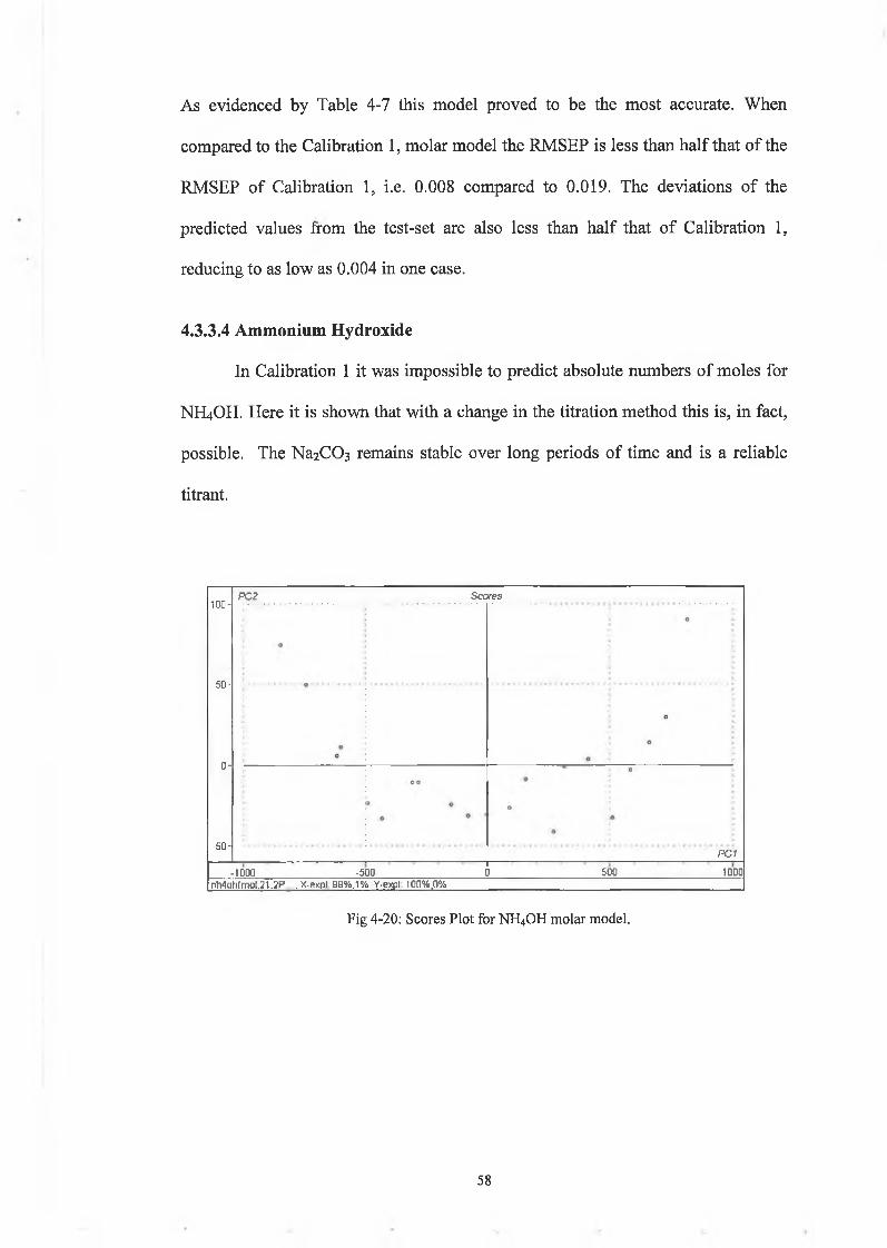
4.3.3.4 Ammonium Hydroxide

In Calibration 1 it was impossible to predict absolute numbers of moles for

NH4OH. Here it is shown that with a change in the titration method this is, in fact,

possible. The Na2C03 remains stable over long periods of time and is a reliable

titrant.

1 0 0 -PC2 Scores

50-

0-

-50-PC1

-1000 -50010 500 1000

r>M(ili[inol.21.2P . X-exol 99%. 1% Y-expl 100%.0%

Fig 4-20: Scores Plot for NH4OH molar model.

5 8

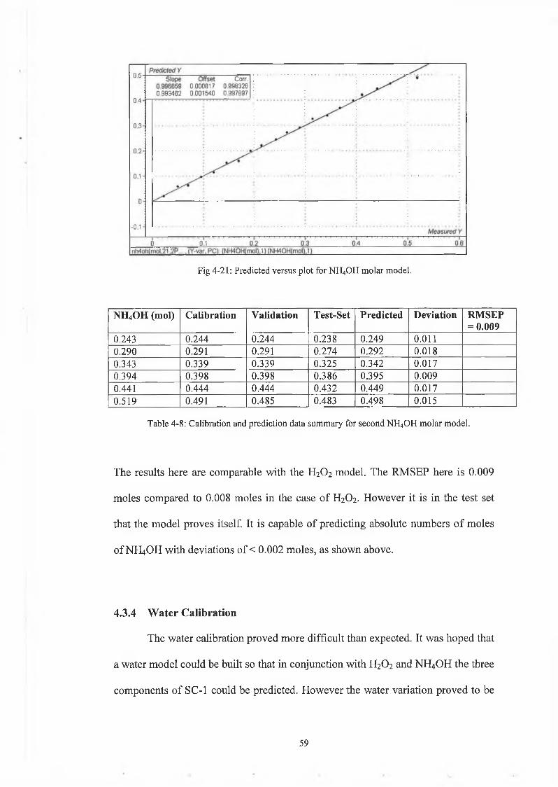
Fig 4-21: Predicted versus plot for NH4OH molar model.

NH4OH (mol) Calibration Validation Test-Set Predicted Deviation RMSEP = 0.009

0.243 0.244 0.244 0.238 0.249 0.0110.290 0.291 0.291 0.274 0.292 0.0180.343 0.339 0.339 0.325 0.342 0.0170.394 0.398 0.398 0.386 0.395 0.0090.441 0.444 0.444 0.432 0.449 0.0170.519 0.491 0.485 0.483 0.498 0.015

Table 4-8: Calibration and prediction data summary for second NH4OH molar model.

The results here are comparable with the H2O2 model. The RMSEP here is 0.009

moles compared to 0.008 moles in the case of H2O2. However it is in the test set

that the model proves itself. It is capable of predicting absolute numbers of moles

of NH4OH with deviations of < 0.002 moles, as shown above.

4.3.4 Water Calibration

The water calibration proved more difficult than expected. It was hoped that

a water model could be built so that in conjunction with H2O2 and NH4OH the three

components of SC-1 could be predicted. However the water variation proved to be

5 9

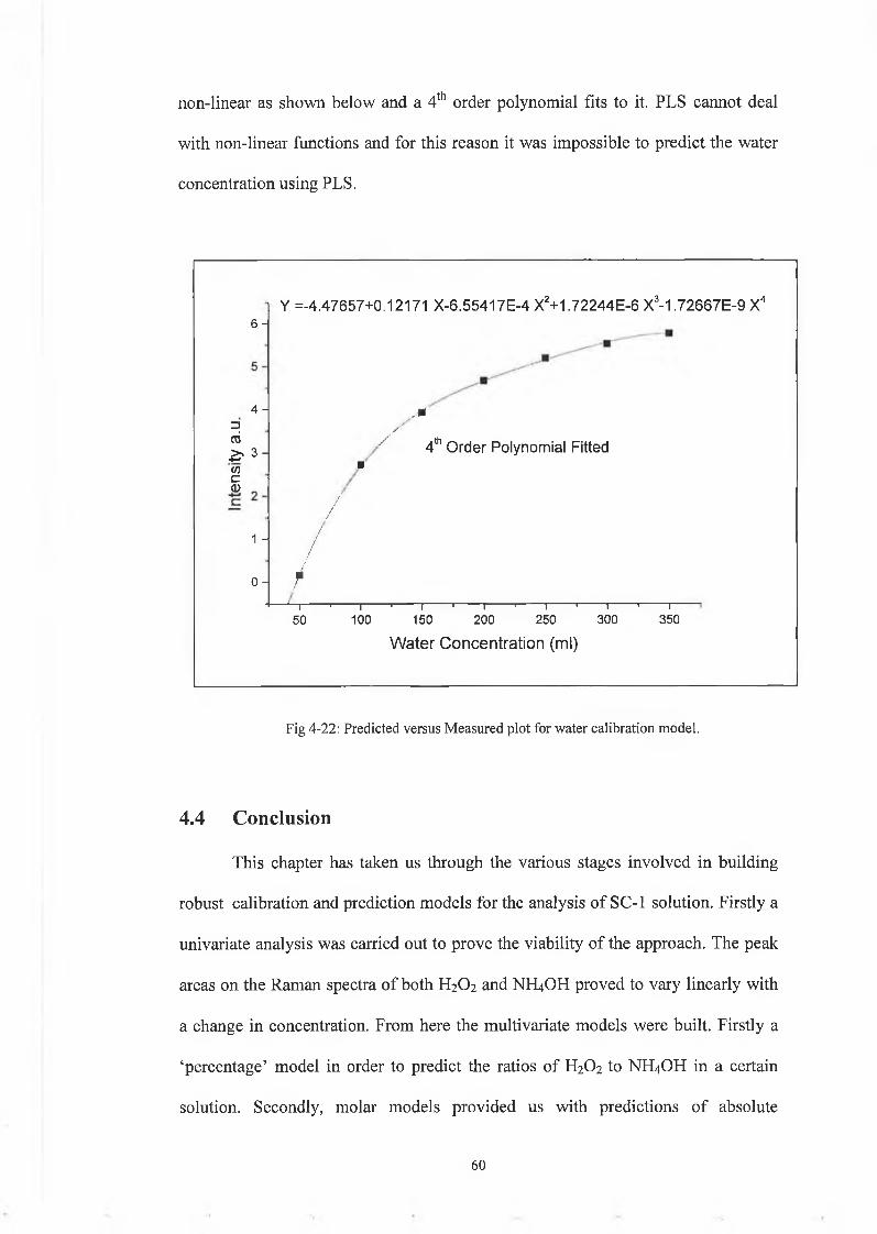
non-linear as shown below and a 4th order polynomial fits to it. PLS cannot deal

with non-linear functions and for this reason it was impossible to predict the water

concentration using PLS.

Y =-4.47657+0.12171 X-6.55417E-4 X2+1.72244E-6 X3-1.72667E-9 X46 -

4 1 ,*=! x03 / ¿th

& 3 - |</jc0)

1 -

0 -

■

//

///

/

4 Order Polynomial Fitted

“i 1---------1---------*---------1---------«---------1--------- '---------1---------t---------i---------1--------- 1—50 100 150 200 250 300 350

W ater Concentration (ml)

Fig 4-22: Predicted versus Measured plot for water calibration model.

4.4 Conclusion

This chapter has taken us through the various stages involved in building

robust calibration and prediction models for the analysis of SC-1 solution. Firstly a

univariate analysis was carried out to prove the viability of the approach. The peak

areas on the Raman spectra of both H2O2 and NH4OH proved to vary linearly with

a change in concentration. From here the multivariate models were built. Firstly a

‘percentage’ model in order to predict the ratios of H2O2 to NFLOFT in a certain

solution. Secondly, molar models provided us with predictions of absolute

6 0

concentrations. The two multivariate calibrations, including ‘percentage’ and

molar models for both of the reagents in SC-1, proved successful except for the

NH4OH molar model in Calibration 1 for reasons outlined in section 4.3.2.4. This

problem was corrected in Calibration 2 and errors were further reduced from

Calibration 1.

61

Chapter 5

Discussion and Conclusions

The aim of this project was to illustrate how Raman spectroscopy combined

with various chemometrics techniques could provide a useful tool for process

control. SC-1 monitoring has become paramount in the semiconductor industry as

both of its main components, hydrogen peroxide (H2O2) and ammonium hydroxide

(NH4OH), degrade and evaporate over time leading to non-uniform processing.

The process control application in question, SC-1 monitoring, is suited to

Raman spectroscopy because of its well-defined spectral peaks. Both H2O2 and

NH4OH produce strong Raman signals at 875cm''(0-0 stretching vibration) and

3315cm''(-NH stretch) respectively. Therefore it was possible to measure peak

areas manually for the univariate approach and for the chemometrics package to

clearly identify the pertinent peaks. In addition to this, Raman signals vary linearly

with a variation in concentration. Therefore, in theory and in practice Raman

spectroscopy was an ideal choice for this application.

Chemometrics has quickly become an invaluable tool for process scientists

as it enables one to build calibration models and thus predict unknowns from these

models. In the SC-1 application chemometrics techniques such as partial least

squares regression (PLSR) helps in building both accurate models and allows for

quick predictions of unknowns.

The principle in question in this project, i.e. is it possible to predict the

concentrations of the individual components of the SC-1 solution spectroscopically,

with the possible exception of water was proved with both univariate and

6 2

multivariate methods with prediction errors as low as 1.17% for both. The

univariate method, however, has no real industrial application, as it proves less

accurate than multivariate methods. This is because multivariate methods take

every data point into account when building models whereas univariate uses only

selected regions of the spectra. However, it does provide the basis for multivariate

analysis and is a useful indicator of the possibilities for different applications. In

this case it illustrated how the peak area varied linearly with concentration.

Multivariate models, however, prove significantly more powerful than

univariate as they take every data point into account. They also predict more

accurately and more easily than univariate and it is in such methods as PLSR and

PCA that the real industrial applications can be seen, as in this case. Chemometrics,

though, is a tool that should be used carefully as it will build models no matter what

is entered. Careful consideration should always be given to the variables used and

to errors in particular. However a model is robust only if independent test sets can

be predicted accurately and also verified. This was the reasoning behind the molar

models as the concentrations predicted could be verified independently of the

calibration model

The presented models show that chemometrics works best with ratios and to

make this project transferable it is imperative that calibrations and predictions are

made on the basis of solution ratios and not absolute volumes. However it was a

valuable exercise to calibrate and predict absolute numbers to enable to

independently verify the concentrations of the components. However it should be

noted that there is danger in working with absolute concentrations as can be seen

from problems encountered with the initial NH4OH molar model. Ratios provide a

simpler, more effective method that ultimately proves more accurate.

6 3

A vital component in this project that proved impossible to predict was the

water concentration. Water as seen in chapter 5 produces a non-linear function and

this precluded PLS from both calibrating and predicting it properly. A 4th order

polynomial was fitted to the data. However it is likely that it is possible to predict it

using a univariate analysis technique.

In principle it has been shown that unknown H2O2 and NH4OH

concentrations can be predicted from calibration models, in the form of both ratios

and absolute concentrations. This could prove invaluable to the semiconductor

industry in terms of uniform processing of wafers, productivity enhancement and

cost reduction. The models illustrated in chapter 4 show excellent accuracy, with

prediction errors of <3% in most cases, and point to the industrial relevance of this

project. Allied to this is the fact that it is a non-invasive technique. Yet, the question

remains whether or not this technique will be transferable to industry. Further

investigations need to be done to incorporate the water concentration into the

models to make this a fully viable industrial application.

6 4

Bibliography

[1] Kern, W. and Puotinen, D.A., RCA Review, 3 1 , pp. 187 (1970).

[2] Kern, J. Electrochem. Soc., 137, 1887 (1990).

[3] Pelletier, M.J., Davis, K. L., Carpio, R.A., Meyappan, M., Economou, D.J.,

Butler, S.W., Proceedings of the Symposium on Process Control,

Diagnostics and Modelling in Semiconductor Manufacturing I.

Electrochem. Soc., pp. 282-293 (1995).

[4] Verhaverbeke, S., Parker, J.W., McConnell, C.F., Proceedings of Materials

Research Society Symposium. 447, p47 (1997).

[5] A.A., Gale, G.W., Kashoush, 1.1., Precision Cleaning, II, p. 13 (1994).

[6] Putterman, S.J. Scientific American, p.46 (Feb 1995).

[7] Zhang, D., Kittleson, D.B., Liu, B., Microcontamination Conf.

Procceedings, San Jose, CA. p.215 (1994).

[8] Itano, M., Kern Jr, F.W., Rosenberg, R.W., Miyashita, M., Kawanabe, I.,

Ohmi, T., IEEE Transactions on Seimconductor Manufacturing, 5, p. 114

(1992).

[9] Kobayshi, H., Ryuta, J., Shingyuji, Shimanuki, Y., Jpn. J. Appi. Phys., 32,

pp. L45-47, Part 2, No. 1A/B (1993).

[10] Meuris, M,, Verhaverbeke, S., Mertens, P.W., Heyns, M.M., Hellemans, L.

Bruynseraede and Philipossian, A., Jpn. J. Appi. Phys., 31, pp. LI 514-1517,

Part 2, No. 11A (1992).

[11] Kaigawa, H., Yamamoto, K., Shigematsu, Y., Jpn. J. Appi. Phys., 33 pp.

4080-4085, Part 1, No. 7A, (1994).

6 5

[12] Kern, W., Semicond. Int., p.94 (1984).

[13] van den Meerakker, J.E.A.M., van der Stratten, M.Y.M., J. Electrochem.

Soc., 137, p.1239(1990).

[14] Tanaka, K , Sakurai, S., Kamizuma, S., Shimanuki, Y., J. Electrochem. Soc.

Ext. Abstr., p.689 (1990).

[15] Tanaka, K., Sakurai, S., Kamizuma, S., Shimanuki, Y., J. Electrochem. Soc.

Ext. Abstr., p.710 (1990).

[16] Sugihara, Y., Shimokawa, S., Oshida, Y., Chemical Proceedings of the

Semiconductor Pure Water and Chemicals Conference, M.J. Balzas, Editr,

Balzas Analytical Laboratory (1993).

[17] Takahashi, I., Kobayshi, H., Ryuta, J., Kishimoto, M., Shingyouji, T., Jpn.

J. Appl. Phys., 32, pp. L1183-L1185, Part 2, No. 9A, (1993).

[18] Carpio, R., Soucy, J., Peterman, S., Jahanbani, M., Electrochem. Soc. Proc,

III, Contamination Control and Defect Reduction in Semiconductor

Manufacturing, (1994).

[19] Barakaev, A.K., Glushkov, S.M., Panchishin, I.M., Zhurnal Prikladnoi

Spektroskopii, 55, p.375 (1991).

[20] Pelletier, M.J., Davis, K.L., Carpio, R.A., Semiconductor International, pp.

103-108 (March 1996).

[21] CS-200 product literature from Horiba Instruments Incorporated, Kyolo,

Japan

[22] D.S. Knight and W.B. White, J. Mater. Res., 4(2), pp.385-393 (1989).

[23] S. Farquharson and S.F. Simpson, Applications of Raman spectroscopy to

industrial processes, SPIE 1681, pp.276-290 (1992).

66

[24] A.M. Tudor, M.C. Davies, C.D. Melia, D.C. Lee, R.C. Mitchell, P.J. Hendra

and S.J. Church, The applications of near infra-red Fourier transform

Raman spectroscopy to the analysis of polymorphic forms of cimetidine,

Spectrochim. Acta., 47A, pp.1389-1393 (1991).

[25] Ingrid De Wolf, Micro Raman spectroscopy to study local mechanical stress

in silicon integrated circuits., Semicond. Sci. Technol., 11, pp. 139-154

(1996).

[26] J.B. Cooper, P.E. Flecher, T.M. Vess and W.T. Welch, Remote fibre-optic

Raman analysis of xylene isomers in mock petroleum fuels using a low cost

dispersive instrument and partial least-square regression analysis, Appl.

Spectrosc., 49, pp.586-592 (1995).

[27] J.B. Cooper, K.L. Wise, J. Groves, and W.T. Welch, Determination of

octane numbers and Reid vapour pressure of commercial petroleum fuels

using FT-Raman spectroscopy and partial least-squares regression analysis,

Anal. Chem., 67, pp.4096-4100 (1995).

[28] Smekal, A., Naturwiss., 11, p.873 (1923).

[29] Practical Raman Spectroscopy, Gardiner, D.J., Graves, P.R., Springer-

Verlag Berlin Heidelberg, (1989).

[30] Behringer, J., The Relation of Resonance Raman Scattering to resonance

Fluouescence, Journal of Raman Spectroscopy, 2(3), pp.275-299 (1974).

[31] Molecular Spectroscopy, 2, The Chemical Society, London (1974).

[32] Baranska, H., Kabudzinska, A., Terpinski, J., Laser Raman Spectrometry,

Analytical Applications, Ellis Horwod Limited, (1987).

[33] Raman, C.V., Nature, pp. 121, 501, 619, 721, (1928).

6 7

[34] Tedesco, J.M.; Owen H., Pallister, D.M., Morris, M.D., Anal. Chem. 65,

p.441A (1993).

[35] Massari, D.L., Vandeginste, B.G.M., Dening, S.M., Michotte, Y., Kaufman

L., Chemometrics: a textbook

[36] Martens, H., Naes T., Multivariate Calibration, Wiley 1989.

[37] Chemometrics for Beginners, Near Infra-Red Publications (NIRP) Training

(May 1998).

6 8

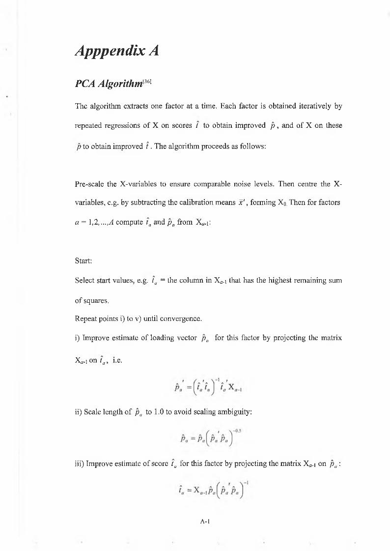
Apppendix A

P C A A l g o r i t h m |36]

The algorithm extracts one factor at a time. Each factor is obtained iteratively by

p to obtain improved i . The algorithm proceeds as follows:

Pre-scale the X-variables to ensure comparable noise levels. Then centre the X-

variables, e.g. by subtracting the calibration means x ' , forming Xo. Then for factors

a = 1,2, ...,A compute ta and p a from X ^:

Start:

Select start values, e.g. ta = the column in Xa.i that has the highest remaining sum

of squares.

Repeat points i) to v) until convergence.

i) Improve estimate of loading vector p a for this factor by projecting the matrix

Xfl-i on ta, i.e.

iii) Improve estimate of score ta for this factor by projecting the matrix Xa_i on p a :

repeated regressions of X on scores t to obtain improved p , and of X on these

ii) Scale length of pa to 1.0 to avoid scaling ambiguity:

A - l

iv) Improve the estimate of the eigenvalue xa :

v) Check convergence: If xa minus ra in the previous iteration is smaller than a

certain small pre-specified constant, e.g. 0.0001 times ra , the method has

converged for this factor. If not go to step i ).

Xa = X a_ , - r aA,'

and go to Start for the next factor.

A-2

Appendix B

P L S 1 A l g o r i t h m [36]

Calibration:

Cl The scaled input variables X and.y are first centered, e.g.

X0 = X - lx 'a n d iy0 = y - ly .

Choose 4max to be higher than the number of phenomena expected in X.

For each factor a= lv ...^4maxperform steps 2.1-2.5:

C 2.1 Use the variability remaining in;' to find the loading weights wa, using least

squares and the local ‘model’.

r

X « - l = y o- i W a + E

and scale the vector to length 1. The solution is

= ¿ C iJV i

where c is the scaling factor that makes the length of the final wa equal to 1, i.e.

C 2.2 Estimate the scores ta using the local ‘model’

tThe LS solution is (since wa wa = 1)

‘ a = X a-\™ a

C 2.3 Estimate the spectral loadings /fusing the local ‘model’

B-l

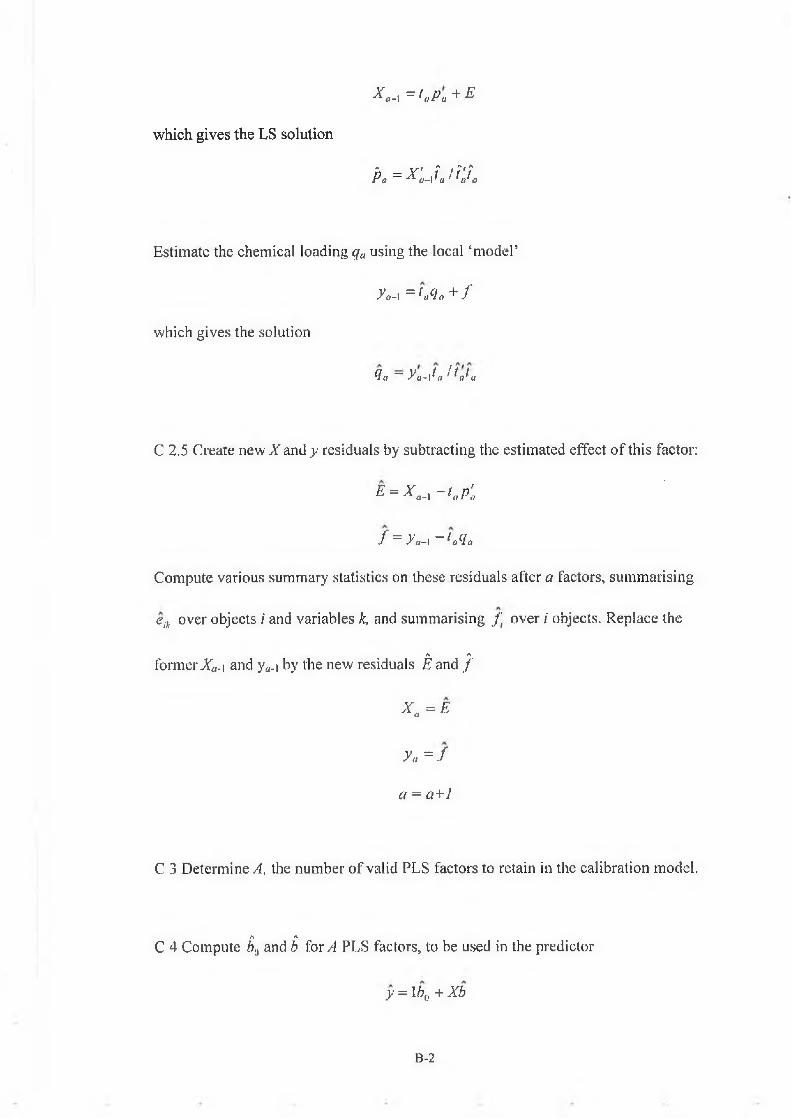
*a-\ = 1 a Pa + ^

/V - «.» * / A # A

P a = K - j J O a

Estimate the chemical loading qa using the local ‘model’

ya-1 =*.?.+/

which gives the solution

9« ~ ya-\ta 11„1 a

which gives the LS solution

C 2.5 Create new X and y residuals by subtracting the estimated effect of this factor:

E = X a_i - t ap'a

f = y a-\ ~K<la

Compute various summary statistics on these residuals after a factors, summarising

e(k over objects i and variables k, and summarising / , over i objects. Replace the

A A

former Xa.\ and y0.i by the new residuals E and /

X a =E

ya = /

a = a+1

C 3 Determine A, the number of valid PLS factors to retain in the calibration model.

A A

C 4 Compute ba and b for A PLS factors, to be used in the predictor

y = \b0 +Xb

B-2

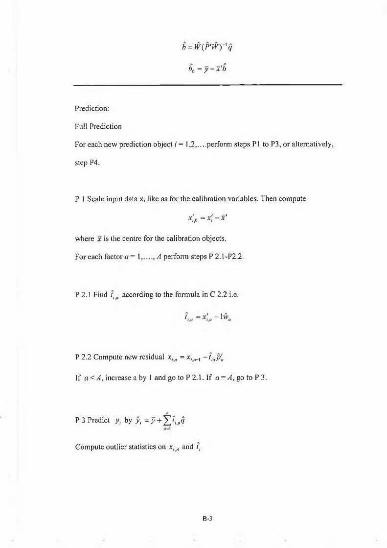
b = iv(P'wy'c]

A A

b0 = y - x b

Prediction:

Full Prediction

For each new prediction object i = 1,2,....perform steps PI to P3, or alternatively,

step P4.

P 1 Scale input data x, like as for the calibration variables. Then compute

<o = x '- x '

where x is the centre for the calibration objects.

For each factor a = 1 A perform steps P 2.1-P2.2.

P 2.1 Find t, a according to the formula in C 2.2 i.e.

P 2.2 Compute new residual x, a = x( 0_, - t lap'a

If a < A, increase a by 1 and go to P 2.1. If a = A, go to P 3.

A

P 3 Predict y, by y, = y + , J

Compute outlier statistics on xi A and (,

B-3

Short Prediction

P 4 Alternatively to steps P 1

y = b0+ x’b

P 3, find y by using b0 and b in C 4, i.e.

B-4