Journal of Neuroscience Methods 146 (2005) 22–41

Applications of multi-variate analysis of variance (MANOVA) tomulti-electrode array electrophysiology data

P.M. Hortona,∗, L. Bonnya, A.U. Nicolb, K.M. Kendrickb, J.F. Fengc,d,∗∗

a Department of Informatics, Sussex University, Falmer, Brighton BN1 9QH, UKb Laboratory of Cognitive and Behavioural Neuroscience, The Babraham Institute, Cambridge CB2 4AT, UK

c Department of Mathematics, Hunan Normal University, 410081, Changsha, PR Chinad Department of Computer Science, Warwick University, Coventry CV4 7AL, UK

Received 11 August 2004; received in revised form 22 November 2004; accepted 13 January 2005

Abstract

We have developed an adaptation of multi-variate analysis of variance (MANOVA) to analyze statistically both local and global patterns ofmulti-electrode array (MEA) electrophysiology data where the activities of many (typically >100) neurons have been recorded simultaneously.Whereas simple application of standard MANOVA techniques prohibits extraction of useful information in this kind of data, our newa logicald om the rato a simplec ed fromh©

K

1

sanDoshgdbnp

j

tion,orks.is iswithviderac-tputndi-eenctiv-

el-t

riatebersthe

nsityarse

0d

pproach, MEANOVA (=MEA+ MANOVA), allows a more useful and powerful approach to analyze such complex neurophysioata. The MEANOVA test enables the detection of the “hot-spots” in the MEA data and has been validated using recordings frlfactory bulb. To further validate the power of this approach, we have also applied the MEANOVA test to data obtained fromomputational network model. This MEANOVA software and other useful statistical methods for MEA data can be downloadttp://www.sussex.ac.uk/Users/pmh20.2004 Elsevier B.V. All rights reserved.

eywords:Multi-electrode array; Multi-variate statistical analysis; Olfactory bulb; Odour; Olfactory bulb modelling

. Introduction

After over a century of neurophysiological research, wetill do not understand the principle by which a stimulus, suchs an odour, an image or a sound, is represented by distributedeural ensembles within the brain (Albright et al., 2000;ayan and Abbott, 2001; Feng, 2004). While large numbersf studies have made detailed analyses of response profiles ofingle cells in isolation, such techniques cannot easily addressolistic issues of how large ensembles of neurones can inte-rate information both spatially and temporally. There is littleoubt that much of the information processing power of therain resides in the activities of co-operating and competingetworks of neurones and that if we can unlock the princi-les whereby information is encoded within these networks

∗ Corresponding author. Tel.: +44 7963 246444; fax: +44 1273 877873.∗∗ Co-corresponding author.E-mail addresses:pmh20@sussex.ac.uk (P.M. Horton),

ianfeng@sussex.ac.uk (J.F. Feng)

as a whole, rather than within single neurones in isolawe may actually be able to understand how the brain w

While some progress towards understanding how thachieved at a gross structural level is being achievedbrain imaging techniques, a promising approach to proan understanding at the level of multiple cell–cell intetions in the brain is the simultaneous recording of the ou(action potentials, spikes) from large numbers of cells ividually within a defined system. This technology has bapplied to an expanding number of studies of neural aity, in both perceptual(Maynard et al., 1999)and cognitive(Johnson and Welsh, 2003) systems, and also in the devopment of implantable neuroprosthetic devices (Patterson eal., 2004; Warwick et al., 2004). The two main difficulties inachieving this step have been, firstly, the lack of approptools to make simultaneous recordings from large numof individual neurones within a network and, secondly,issue of analysing the resulting huge amount of high-demulti-variate data, in which significant effects may be spacross the large sample of neurons.

165-0270/$ – see front matter © 2004 Elsevier B.V. All rights reserved.oi:10.1016/j.jneumeth.2005.01.008

P.M. Horton et al. / Journal of Neuroscience Methods 146 (2005) 22–41 23

A small number of groups have now developed the nec-essary recording hardware and software tools for data acqui-sition and these are available commercially (e.g. Plexon Inc.and Cyberkinetics Inc., USA). Currently, however, even withsome data compression algorithms, recordings from 128 elec-trodes sampled at 100 kHz routinely produce around 15 MBof data/min. With most individual experimental sessions last-ing several hours or more this can produce data sets of manyhundreds of GB. There are a number of software analyticalpackages for editing and visualising data using raster/eventplots or pseudocolour grids, and it is possible to provide arelatively cursory analysis of this high volume data usinggeneric programmes (e.g. Matlab, NeuroExplorer, Spike2).However, there is very little that has been developed for de-tailed statistical analysis, and subsequent visual representa-tion of the changing spatial and temporal patterns of infor-mation recorded across the electrode arrays.

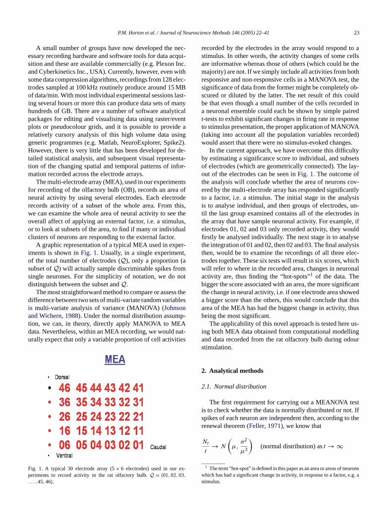
The multi-electrode array (MEA), used in our experimentsfor recording of the olfactory bulb (OB), records an area ofneural activity by using several electrodes. Each electroderecords activity of a subset of the whole area. From this,we can examine the whole area of neural activity to see theoverall affect of applying an external factor, i.e. a stimulus,or to look at subsets of the area, to find if many or individualclusters of neurons are responding to the external factor.

A graphic representation of a typical MEA used in exper-i t,o as ms notd

s thed blesia p-t Ad nat-u ies

F x-p.

recorded by the electrodes in the array would respond to astimulus. In other words, the activity changes of some cellsare informative whereas those of others (which could be themajority) are not. If we simply include all activities from bothresponsive and non-responsive cells in a MANOVA test, thesignificance of data from the former might be completely ob-scured or diluted by the latter. The net result of this couldbe that even though a small number of the cells recorded ina neuronal ensemble could each be shown by simple pairedt-tests to exhibit significant changes in firing rate in responseto stimulus presentation, the proper application of MANOVA(taking into account all the population variables recorded)would assert that there were no stimulus-evoked changes.

In the current approach, we have overcome this difficultyby estimating a significance score to individual, and subsetsof electrodes (which are geometrically connected). The lay-out of the electrodes can be seen inFig. 1. The outcome ofthe analysis will conclude whether the area of neurons cov-ered by the multi-electrode array has responded significantlyto a factor, i.e. a stimulus. The initial stage in the analysisis to analyse individual, and then groups of electrodes, un-til the last group examined contains all of the electrodes inthe array that have sample neuronal activity. For example, ifelectrodes 01, 02 and 03 only recorded activity, they wouldfirstly be analysed individually. The next stage is to analysethe integration of 01 and 02, then 02 and 03. The final analysist lec-t hichw ronala eb ificantt oweda t thisa thusb

us-i linga dours

2

2

sti t. Ifs to ther

uronsw e.g. as

ments is shown inFig. 1. Usually, in a single experimenf the total number of electrodes (Q), only a proportion (ubset ofQ) will actually sample discriminable spikes froingle neurones. For the simplicity of notation, we doistinguish between the subset andQ.

The most straightforward method to compare or assesifference between two sets of multi-variate random varia

s multi-variate analysis of variance (MANOVA) (Johnsonnd Wichern, 1988). Under the normal distribution assum

ion, we can, in theory, directly apply MANOVA to MEata. Nevertheless, within an MEA recording, we wouldrally expect that only a variable proportion of cell activit

ig. 1. A typical 30 electrode array (5× 6 electrodes) used in our eeriments to record activity in the rat olfactory bulb.Q = {01,02,03,. . ,45,46}.

hen, would be to examine the recordings of all three erodes together. These six tests will result in six scores, will refer to where in the recorded area, changes in neuctivity are, thus finding the “hot-spots”1 of the data. Thigger the score associated with an area, the more sign

he change in neural activity, i.e. if one electrode area shbigger score than the others, this would conclude tharea of the MEA has had the biggest change in activity,eing the most significant.

The applicability of this novel approach is tested hereng both MEA data obtained from computational modelnd data recorded from the rat olfactory bulb during otimulation.

. Analytical methods

.1. Normal distribution

The first requirement for carrying out a MEANOVA tes to check whether the data is normally distributed or nopikes of each neuron are independent then, accordingenewal theorem(Feller, 1971), we know that

Nt

t→ N

(µ,

σ2

µ3

)(normal distribution) ast → ∞

1 The term “hot-spot” is defined in this paper as an area or areas of nehich has had a significant change in activity, in response to a factor,timulus.

24 P.M. Horton et al. / Journal of Neuroscience Methods 146 (2005) 22–41

whereµ is the mean interspike interval,σ2 the variance andNt is the spike counting inside time window [0, t]. The inde-pendent assumption can be relaxed and replaced by a weak as-sumption: the spike train is stationary. Of course, the station-ary assumption is still a strong requirement for many cases.For example, in the MEA data from the olfactory bulb, it isclear that habituation is a common phenomenon and occursover an even smaller time scale than the recording periodused for analysis (5–10 s). There are a few ways to overcomethe difficulty. For example, when we calculateNt , we couldintroduce weights for different interspike intervals, a typicalde-trend method, and so on.

Of course, in the data from our modelling approach, sincethe interspike intervals are generated from an integrate-and-fire model, the interspike intervals are perfectly renewal pro-cesses. Hence, all our results hold true. For multi-dimensionalrenewal theorem, we refer the reader toHunter (1974a,b).

For experimental data, as far as we can tell, all statisticalapproaches including the one we developed here are validonly to a certain degree. For example, even for an in vivorecording from a single cell, we know its output is no longera stationary process. Hence, the assumption for a routine sta-tistical test such ast-test or Komogrov test fails.

However, up to date it is difficult, if not impossible, tosimulate the local field potential, since we do not know thee e finar it ons

2

rstr ofo r-r((t wF .I oft

N

w noa

uso andd(j

w

X

whereµ is the mean vector,F1 the effect of the first fac-tor, for example, stimulus factor,F2 the effect of the secondfactor, for example, trial factor,F1,2 the interaction betweenthe two factors,ξ a normally distributed random vector withmean zero,i = 1, . . . , I, j = 1, . . . , J andm = 1, . . . ,M isthe number of samplings. In other words,Xijm is a samplingofNm, that is,Xijm is the array activity ofmth window. NotethatXijm is aP-dimensional random vector. For simplicityof notation, let us further introduce that

X̄i· =J∑

j=1

M∑m=1

Xijm

JM, (2.2)

X̄·j =I∑

i=1

M∑m=1

Xijm

IM, (2.3)

X̄ij =M∑

m=1

Xijm

M, (2.4)

X̄ =I∑

i=1

J∑j=1

M∑m=1

Xijm

IJM(2.5)

whereX̄ is the average of all the observations,X̄i· the averageoa2 thei s.(t wlyd

X

d bye undri ev et ter-a evelso , ifa oulds trial2 dew

t ac-c nteda iduale weres erva-t ctorsa

xact sources to generate it; hence, we can not check thesults using modelling approach. Here, we only usepiking data.

.2. Two-way MANOVA

For a particular experiment, for example, with the fiecording trial with exposure to a fixed concentrationdour, let us assume that we haveQ electrodes in the aay and have recorded the activity ofP cells. Let Y =yp,q, p = 1, . . . , P), q ∈ Q are spike trains withyp,q =tkp,q, k = 1, . . . , Kp,q), wheretkp,q is thekth spike andKp,q ishe total number of spikes within the recorded time windoT.or a given bin sizet, we can divideT intoM = T/t time bins

nside each time bin, letNmp,q represent the spike counting

hemth window,m = 1, . . . ,M = T/t. Hence, we have

m = {Nmp,q,m = 1, . . . , T/t, p = 1, . . . , P}, q ∈ Q

hich is a normally distributed,p-dimensional vector. Ither words, we have a random vectorN with P dimensionsndM = T/t samplings (replicates).

The random vectorNm is usually dependent on variother factors. If we have two sampling periods (pre-uring-stimulus presentation) over three trials, we havei = 1pre-stimulus) andi = 2 (during stimulus),j = 1 (trial 1),= 2 (trial 2) andj = 3 (trial 3). For each fixedi, j andm,e have

ijm = µ + F1i + F2

j + F1,2ij + ξijm (2.1)

l f the observation vectors at theith level of factor 1,X̄·j theverage of the observation vectors at thejth level of factorandX̄ij is the average of the observation vectors at

th level of factor 1 and thejth level of factor 2. From Eq2.2) to (2.5), we can decompose the equation above in(2.1)o describeXijm the observational vector, using the neefined variables.

ijm = X̄ + (X̄i· − X̄) + (X̄·j − X̄)

+ (X̄ij − X̄i· − X̄·j + X̄) + (Xijm − X̄ij) (2.6)

This equation shows how the observed result is achievexamining the factors which have contributed to get the foesult, i.e. how much factor 1 (̄Xi· − X̄), factor 2 (X̄·j − X̄),nteraction (̄Xij − X̄i· − X̄·j + X̄) and the remainder of thariance (residual error) (Xijm − X̄ij) have contributed to thotal variance, thus resulting in the observation. The inction describes the relationship between the various lf factors 1 and 2. An example of interaction would bestimulus was presented in three trials, trials 1 and 3 c

how an increase in activity but a decrease was shown in. If this was the case, it would be very difficult to concluhat the affect of the factors were.The residual error describes the variance which is no

ountable by either factor 1 or 2. If a stimulus was presend the result of this was that the variance of the resrror was large and the variances of factors 1 and 2mall, would conclude that the chances are that the obsion recorded has been caused by unknown (random) fand not by either of the factors under examination.

P.M. Horton et al. / Journal of Neuroscience Methods 146 (2005) 22–41 25

2.3. MEANOVA = MEA + MANOVA

According to the classical MANOVA (Johnson and Wich-ern, 1988), we see that we should calculate the followingmatrices:

S1 =I∑

i=1

JM(X̄i· − X̄)(X̄i· − X̄)′ (2.7)

S2 =J∑

j=1

IM(X̄·j − X̄)(X̄·j − X̄)′ (2.8)

S3 =I∑

i=1

J∑j=1

M(X̄ij − X̄i· − X̄·j + X̄)

× (X̄ij − X̄i· − X̄·j + X̄)′ (2.9)

Sr =I∑

i=1

J∑j=1

M∑m=1

(Xijm − X̄ij)(Xijm − X̄ij)′ (2.10)

whereS1 is the residual error due to the first factor,S2 theresidual error due to the second factor,S3 the residual errordue to the interaction between the first factor and the sec-o thei tors( tivity.T

Λ

Λ

r1 t theh thec

chi-s t thec s andnt hy-p tionsi

−

-si

.t r the

factors 1 and 2.2 We reject the hypothesis that there is nosignificant change due to factor 1 if

−∣∣∣∣IJ(M − 1) − P + 1 − (I − 1)

2

∣∣∣∣ ln Λ1 > χ2(I−1)P (α),

(2.13)

whereχ2(I−1)(J−1)P (α) is the upper (100α) percentile of a chi-

squared distribution with (I − 1)P(α)d.f. The significancelevel (α) of 5% was used for all factor 1 tests.

We reject the hypothesis that there are no significantchanges due to factor 2 if

−∣∣∣∣IJ(M − 1) − P + 1 − (J − 1)

2

∣∣∣∣ ln Λ2 > χ2(J−1)P (α).

(2.14)

whereχ2(J−1)P (α) is the upper (100α) percentile of a chi-

square distribution with (I − 1)p(α)d.f. The significancelevel (α) of 5% was used for all factor 2 tests.

Unfortunately, the text book version of MANOVA cannot be directly applied to our MEA data. For example, asshown inFig. 10 bottom panel right, if we simply put allrecorded neurons in our analysis, we will simply concludethat there is no significant change between pre- and duringstimulus (see below for more details). The other reason ist des)i ntlyc .

ne as

S

S

S

desi

fromd tic

k/U

nd factor andSr is the total residual. The next stage innterpretation is to test the likelihood that any of the facinteractions, factor 1 or 2) caused a change in neuron achis is acheived by using Wilks’ lambda.

3 = |Sr||S3 + Sr| Λ1 = |Sr|

|S1 + Sr|

2 = |Sr||S2 + Sr| . (2.11)

Intuitively, whenΛi, i = 1,2,3, is small, the factor (facto, 2 or the interaction) is important and so we can rejecypothesis that the factor is negligible. This is exactlyase in MANOVA.

For large samples, Wilks’ lambda can be used with aquared percentile, to provide us with confidence thahange in the results was due to the factors, i.e. a stimuluot by chance. Using Barletts multiplier(Bartletts, 1954),

o improve the chi-squared approximation, we reject theothesis that there are no significant changes in interac

f ∣∣∣∣IJ(M − 1) − P + 1 − (I − 1)(J − 1)

2

∣∣∣∣× ln Λ3 > χ2

(I−1)(J−1)P (α) (2.12)

whereχ2(I−1)(J−1)P (α) is the upper (100α) percentile of a chi

quared distribution with (I − 1)(B − 1)P(α)d.f. The signif-cance level (α) of 5% was used for all interaction tests.

Under the circumstances that Eq.(2.12) is not true, i.ehe interaction is not strong enough. We can then test fo

hat we intend to detect the hottest spot (group of electron experiments, i.e. the group of neurons most significahanged in response to stimulus or due to other factors

With the above considerations in mind, we can defiignificant score for a subsetS of Q as

3(S) = −∣∣∣∣IJ(M − 1) − |S| + 1 − (I − 1)(J − 1)

2

∣∣∣∣× ln Λ3

χ2(I−1)(J−1)|S|(α)

, (2.15)

1(S) = −∣∣∣∣IJ(M − 1) − |S| + 1 − (I − 1)

2

∣∣∣∣× ln Λ1

χ2(I−1)|S|(α)

, (2.16)

2(S) = −∣∣∣∣IJ(M − 1) − |S| + 1 − (J − 1)

2

∣∣∣∣× ln Λ2

χ2(J−1)|S|(α)

, (2.17)

where|S| is the number of neurons recorded by electron S. It is routinely required thatIJ(M − 1) > |S|.

Please note that the significant score is made upividing the improved Wilks’ lambda with the test statis

2 One-way MEANOVA is available at http://www.sussex.ac.users/pmh20.

26 P.M. Horton et al. / Journal of Neuroscience Methods 146 (2005) 22–41

drawn from theχ2 distribution. A score of 1 and over will bedeemed as significant at the 5% significance level, i.e. we have95% confidence that the results, which have been affected aredue to one of the observed factors such as a presented stim-ulus. The higher the significance score the bigger the changein results, i.e. the bigger the change in neural activity.

Therefore, a subsetS which attains the highest value ofthe significant score is the ‘hottest spot’ in the array. Thehottest spots reveal the groups of neurons with most signifi-cant changes.

3. Modelling approach

An olfactory bulb model was created, adopted from a sim-ple model3 (Margrie and Schaefer, 2003), for the main pur-pose of proving that the MEANOVA approach works. Toprove this, particular mitral cells (MCs) are chosen to in-crease their activity in response to stimulus presentation, sothe cells responding most significantly will already be knownto us. MEANOVA will then be used on the spiking data cre-ated from the cells, to see if it yields the expected results, i.e.the chosen and surrounding mitral cells should have the mostsignificant change in activity.

To achieve this, two sets of mitral cell data are needed,t lusp ed byM

ings e re-m howt ctiv-i uldb tions uronsr sec-t

3

6.5( stso con-n lleda hownb

τ

T tingp her

The input (Ie) is in the form of:

Ie = 4 Hz oscillation current+ fixed current

A 4 Hz oscillatory current is injected into each of the mi-tral cells with a peak amplitude of 125 pA. This mimickedseveral sniff cycles. Each mitral cell also had a constant cur-rent, chosen randomly in the range of [0.265,0.27] nA at theoutset of the experiment injected into it. Thus, each mitralcell differed slightly from the rest. The range needed to besmall, to make all trials similar. This would ensure, that thehot areas, across the array would be similar across trials. Witha larger range, the random inputs to each neuron in each trial,could vary greatly, thereby influencing the final interactionresults, i.e. producing results larger than 1.

The final input to all mitral cells, is a postsynaptic current.The strength of the connection (conductance) corresponds tothe value ofgs. All connection strengths for all mitral cellswere 5 S (siemens). To produce an inhibitory effect on theconnection, reversal potential (Es) was set to−10 mV. Foran excitatory connection, this was set to 35 mV.

Each mitral cell was connected to eight surrounding cells,for example inFig. 1, cell 23 is connected to cells 12, 13,14, 22, 24, 32, 33 and 34. Non-target cells which are notconnected to the target cells have reciprocal inhibitory con-n t cellh rgetc tar-g fect.T

du

P

T aso is,t inge

τ

w xci-t and6

lec-t hasti imei te as itralc

-c f2 here

o show the activity of the cells, before and during-stimuresentation. These two sets of data can then be usEANOVA to calculate the significant scores.Three trials will be used, with the activity of the cells be

imilar in each, and the mitral cells chosen as responsivaining unchanged throughout. This is implemented to s

hat in different trials the same neurons change their aty, in response to stimulus presentation. MEANOVA woe used to help prove or disprove this, i.e. if the interaccores are below 1, it has been shown that particular neespond to a particular stimulus. The following two subions, discuss the model used, and the results gained.

.1. Network model used

Simulations were created and performed in MatlabThe MathWorks, Natick, MA, USA). The network consif a connected set of mitral cells where each mitral cell isected to all of the adjacent ones. Mitral cells were modes leaky integrate-and-fire neurons, the equation is selow:

m · dV

dt= El − V − gs · Ps · (V − Es) + Rm · Ie + noise

he cells had an action potential threshold of 15 mV, resotential (El ) of 12 mV, τm = 10 ms and noise was in tange of [0,0.005] nA.Rm had the value of 1 M%.

3 We have developed biophysical models inDavison et al. (2003).

ections. Non-target cells which are connected to a targeave either an excitatory connection to them from the taell, forming a cluster of heightened activity around theet, or an inhibitory connection to produce the opposite efarget cells always receive an excitatory connection.

The synaptic open probability (Ps) variable was modellesing the following:

→ Ps + Pmax(1 − Ps)

his is the state ofPs after a pre-synaptic action potential hccurred,Pmax having the value of 1. Immediately after th

he variable decays exponentially to zero, using the followquation:

s · dPs

dt= −Ps

hereτs is the time constant for the connection. The eatory and inhibitory values for the connections was 2ms, respectively.For the purposes of MEANOVA, in this section, one e

ode corresponds to a single mitral cell. Each electrodehe same labelling and layout as shown inTable 1. The spik-ng activity of all the cells was recorded over a range of tntervals, and a varying number of time bins. To creatimulus, another input was injected into the chosen mells.

The stimulus starts from timet at 0 nA and steadily inreases over a time period of (t + duration)/2 to a peak o5 nA. The stimulus then steadily decreases to 0 nA w

P.M. Horton et al. / Journal of Neuroscience Methods 146 (2005) 22–41 27

Table 1This table shows the neurons in the a 4× 4 layout

01 02 03 0411 12 13 1421 22 23 2431 32 33 34

The target neurons are shown in italic.

the final time oft + duration is reached (duration for thispaper was 0.5 s). This was used to simulate an increase anddecrease of odour concentration. This was used to inducehot-spots, i.e. a change in activity, into the selected mitralcells.

Two experiments were constructed to show theMEANOVA results, for a small and a large group of data,i.e. a small and a large array of neurons.

1. The number of mitral cells used to gain the results in thefirst experiment was 16, i.e. a 4× 4 array. This is shownin Table 1.

2. The second experiment used a 9× 9 array, and showsthat MEANOVA can pick out a few significantly changedneurons from a very large group. The stimulus is alsodecreased to a peak of 20 nA, to show the affects it has onthe significant scores.

3.2. Results generated from model for first experiment

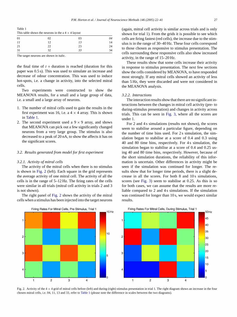
3.2.1. Activity of mitral cellsThe activity of the mitral cells when there is no stimulus

is shown inFig. 2 (left). Each square in the grid representsthe average activity of one mitral cell. The activity of all thecells is in the range of 5–12 Hz. The firing rates of the cellswere similar in all trials (mitral cell activity in trials 2 and 3i

lc urons

(again, mitral cell activity is similar across trials and is onlyshown for trial 1). From the grids it is possible to see whichcells are firing fastest (red cells), the increase due to the stim-ulus is in the range of 30–40 Hz. These four cells correspondto those chosen as responsive to stimulus presentation. Thecells surrounding these responsive cells also show increasedactivity, in the range of 15–20 Hz.

These results show that some cells increase their activityin response to stimulus presentation. The next few sectionsshow the cells considered by MEANOVA, to have respondedmost strongly. If any mitral cells showed an activity of lessthan 5 Hz, they were discarded and were not considered inthe MEANOVA analysis.

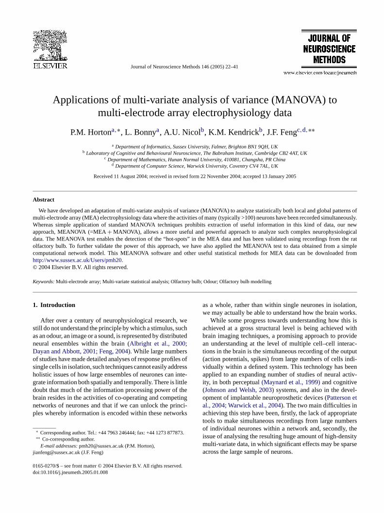
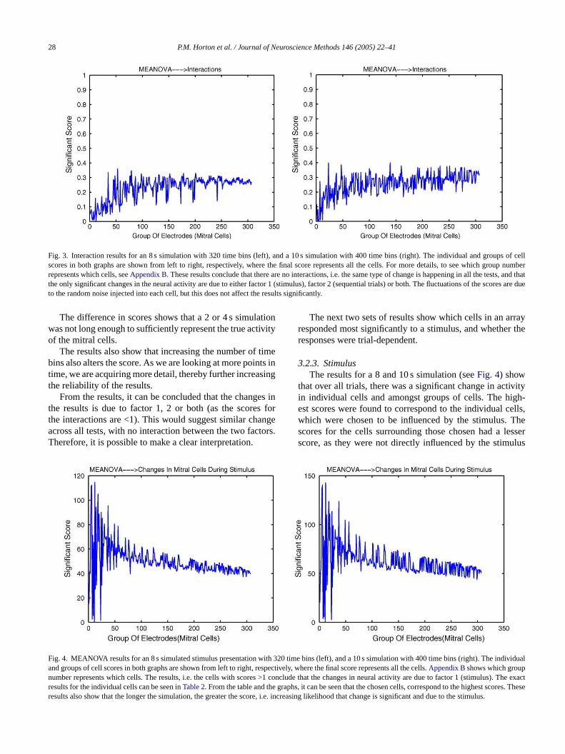
3.2.2. InteractionsThe interaction results show that there are no significant in-

teractions between the changes in mitral cell activity (pre- toduring-stimulus presentation) and changes in activity acrosstrials. This can be seen inFig. 3, where all the scores areunder 1.

For 2 and 4 s simulations (results not shown), the scoresseem to stabilise around a particular figure, depending onthe number of time bins used. For 2 s simulation, the sim-ulation began to stabilise at a score of 0.4 and 0.3 using40 and 80 time bins, respectively. For 4 s simulation, thesimulation began to stabilise at a score of 0.4 and 0.25 us-i e oft or-m bes re-s de-c ions,s sof re re-l tionw ilarr

F ight) st the fourc differe

s not shown).The right panel ofFig. 2 shows the activity of the mitra

ells when a stimulus has been injected into the target ne

ig. 2. Activity of the 4× 4 grid of mitral cells before (left) and during (rhosen mitral cells, i.e. 04, 11, 13 and 33, refer toTable 1(please note the

ng 40 and 80 time bins, respectively. However, becaushe short simulation durations, the reliability of this infation is uncertain. Other differences in activity might

een if the simulation was continued for longer. Theults show that for longer time periods, there is a slightrease in all the scores. For both 8 and 10 s simulatcores (seeFig. 3) seem to stabilise at 0.25. As this isor both cases, we can assume that the results are moiable compared to 2 and 4 s simulations. If the simulaas continued for longer than 10 s, we would expect sim

esults.

imulus presentation in trial 1. The right diagram shows an increase innce in scales between the two diagrams).

28 P.M. Horton et al. / Journal of Neuroscience Methods 146 (2005) 22–41

Fig. 3. Interaction results for an 8 s simulation with 320 time bins (left), and a 10 s simulation with 400 time bins (right). The individual and groups ofcellscores in both graphs are shown from left to right, respectively, where the final score represents all the cells. For more details, to see which group numberrepresents which cells, seeAppendix B. These results conclude that there are no interactions, i.e. the same type of change is happening in all the tests, and thatthe only significant changes in the neural activity are due to either factor 1 (stimulus), factor 2 (sequential trials) or both. The fluctuations of the scores are dueto the random noise injected into each cell, but this does not affect the results significantly.

The difference in scores shows that a 2 or 4 ssimulationwas not long enough to sufficiently represent the true activityof the mitral cells.

The results also show that increasing the number of timebins also alters the score. As we are looking at more points intime, we are acquiring more detail, thereby further increasingthe reliability of the results.

From the results, it can be concluded that the changes inthe results is due to factor 1, 2 or both (as the scores forthe interactions are <1). This would suggest similar changeacross all tests, with no interaction between the two factors.Therefore, it is possible to make a clear interpretation.

The next two sets of results show which cells in an arrayresponded most significantly to a stimulus, and whether theresponses were trial-dependent.

3.2.3. StimulusThe results for a 8 and 10 s simulation (seeFig. 4) show

that over all trials, there was a significant change in activityin individual cells and amongst groups of cells. The high-est scores were found to correspond to the individual cells,which were chosen to be influenced by the stimulus. Thescores for the cells surrounding those chosen had a lesserscore, as they were not directly influenced by the stimulus

F ith 320 ndivia specti pn >1 con s). Ttr e grap res. Theser , i.e. in

ig. 4. MEANOVA results for an 8 s simulated stimulus presentation wnd groups of cell scores in both graphs are shown from left to right, reumber represents which cells. The results, i.e. the cells with scoresesults for the individual cells can be seen inTable 2. From the table and thesults also show that the longer the simulation, the greater the score

time bins (left), and a 10 s simulation with 400 time bins (right). The idualvely, where the final score represents all the cells.Appendix Bshows which grouclude that the changes in neural activity are due to factor 1 (stimuluhe exachs, it can be seen that the chosen cells, correspond to the highest scocreasing likelihood that change is significant and due to the stimulus.

P.M. Horton et al. / Journal of Neuroscience Methods 146 (2005) 22–41 29

but by the connection strengths between them and the chosencells.

The results show that the simulation results stabilise at ascore of 50. This is not so in simulations of 2 and 4 s (resultsnot shown), where the scores were not similar and so wereless reliable.

These results show that the longer the simulation, thegreater the score, i.e. increasing likelihood that change issignificant.

MEANOVA clearly shows that the neurons with the mostsignificant change are those selected to respond to the stim-ulus (seeTable 2).

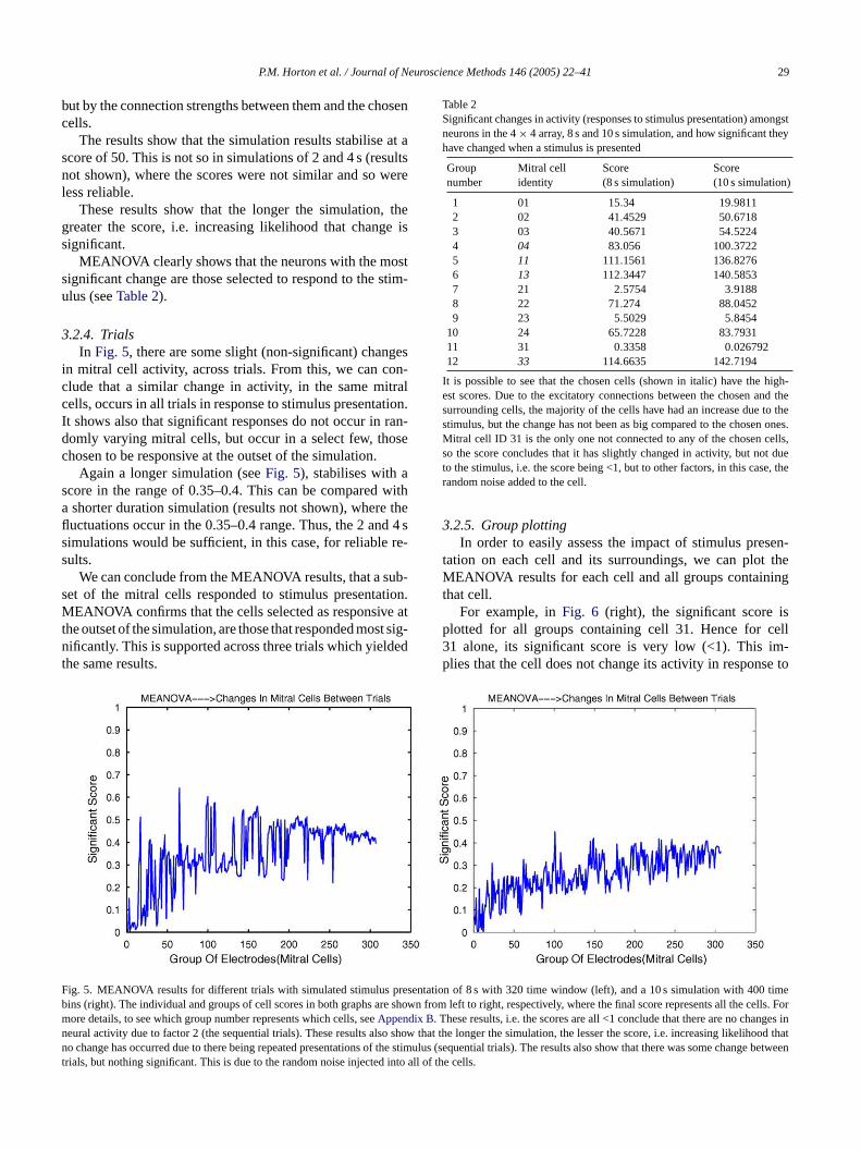
3.2.4. TrialsIn Fig. 5, there are some slight (non-significant) changes

in mitral cell activity, across trials. From this, we can con-clude that a similar change in activity, in the same mitralcells, occurs in all trials in response to stimulus presentation.It shows also that significant responses do not occur in ran-domly varying mitral cells, but occur in a select few, thosechosen to be responsive at the outset of the simulation.

Again a longer simulation (seeFig. 5), stabilises with ascore in the range of 0.35–0.4. This can be compared witha shorter duration simulation (results not shown), where thefluctuations occur in the 0.35–0.4 range. Thus, the 2 and 4 ss re-s

ub-s tion.M e att st sig-n ldedt

Table 2Significant changes in activity (responses to stimulus presentation) amongstneurons in the 4× 4 array, 8 s and 10 s simulation, and how significant theyhave changed when a stimulus is presented

Groupnumber

Mitral cellidentity

Score(8 s simulation)

Score(10 s simulation)

1 01 15.34 19.98112 02 41.4529 50.67183 03 40.5671 54.52244 04 83.056 100.37225 11 111.1561 136.82766 13 112.3447 140.58537 21 2.5754 3.91888 22 71.274 88.04529 23 5.5029 5.8454

10 24 65.7228 83.793111 31 0.3358 0.02679212 33 114.6635 142.7194

It is possible to see that the chosen cells (shown in italic) have the high-est scores. Due to the excitatory connections between the chosen and thesurrounding cells, the majority of the cells have had an increase due to thestimulus, but the change has not been as big compared to the chosen ones.Mitral cell ID 31 is the only one not connected to any of the chosen cells,so the score concludes that it has slightly changed in activity, but not dueto the stimulus, i.e. the score being <1, but to other factors, in this case, therandom noise added to the cell.

3.2.5. Group plottingIn order to easily assess the impact of stimulus presen-

tation on each cell and its surroundings, we can plot theMEANOVA results for each cell and all groups containingthat cell.

For example, inFig. 6 (right), the significant score isplotted for all groups containing cell 31. Hence for cell31 alone, its significant score is very low (<1). This im-plies that the cell does not change its activity in response to

F presen 00 timeb e show rm dix B. T nges inn o shown the sti hanget into al

imulations would be sufficient, in this case, for reliableults.

We can conclude from the MEANOVA results, that a set of the mitral cells responded to stimulus presentaEANOVA confirms that the cells selected as responsiv

he outset of the simulation, are those that responded moificantly. This is supported across three trials which yie

he same results.

ig. 5. MEANOVA results for different trials with simulated stimulusins (right). The individual and groups of cell scores in both graphs arore details, to see which group number represents which cells, seeAppeneural activity due to factor 2 (the sequential trials). These results also change has occurred due to there being repeated presentations of

rials, but nothing significant. This is due to the random noise injected

tation of 8 s with 320 time window (left), and a 10 s simulation with 4n from left to right, respectively, where the final score represents all the cells. Fohese results, i.e. the scores are all <1 conclude that there are no chathat the longer the simulation, the lesser the score, i.e. increasinglikelihood that

mulus (sequential trials). The results also show that there was some cbetweenl of the cells.

30 P.M. Horton et al. / Journal of Neuroscience Methods 146 (2005) 22–41

Fig. 6. Group plot of MEANOVA results.Left: significant score for all 12 cells and their associated groups.Right, significant score for cell 31. Hence, the firstpoint corresponds to 31, the second point to 23= (21,31), the third point to 37= (11,21,31), etc. (seeAppendix B).

stimulus presentation. However, when considered togetherwith cell 21, its significant score is 2.5, i.e. there is asignificant response to stimulus presentation for the group(21,31).

3.3. Results generated from model for secondexperiment

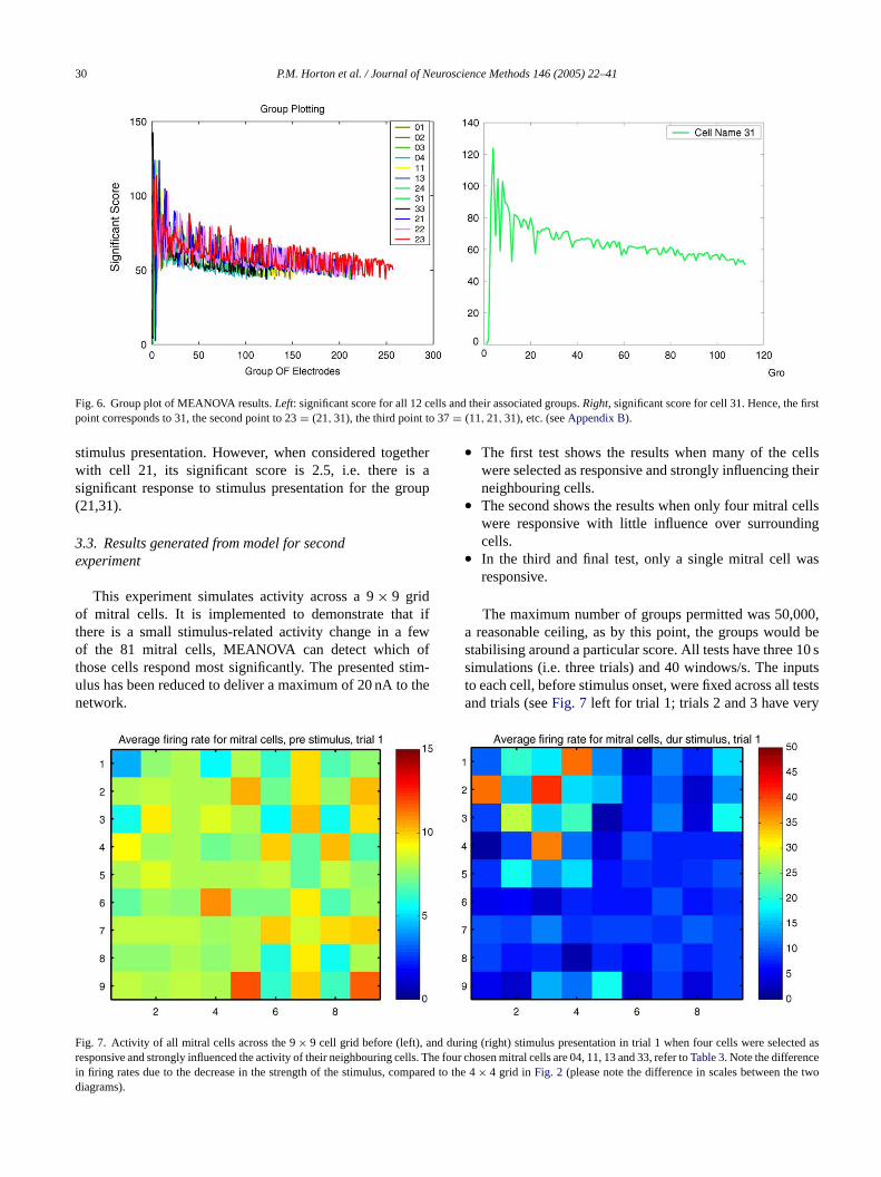
This experiment simulates activity across a 9× 9 gridof mitral cells. It is implemented to demonstrate that ifthere is a small stimulus-related activity change in a fewof the 81 mitral cells, MEANOVA can detect which ofthose cells respond most significantly. The presented stim-ulus has been reduced to deliver a maximum of 20 nA to thenetwork.

• The first test shows the results when many of the cellswere selected as responsive and strongly influencing theirneighbouring cells.

• The second shows the results when only four mitral cellswere responsive with little influence over surroundingcells.

• In the third and final test, only a single mitral cell wasresponsive.

The maximum number of groups permitted was 50,000,a reasonable ceiling, as by this point, the groups would bestabilising around a particular score. All tests have three 10 ssimulations (i.e. three trials) and 40 windows/s. The inputsto each cell, before stimulus onset, were fixed across all testsand trials (seeFig. 7 left for trial 1; trials 2 and 3 have very

F and du cted asr lls. The ei mpared twod

ig. 7. Activity of all mitral cells across the 9× 9 cell grid before (left),esponsive and strongly influenced the activity of their neighbouring cen firing rates due to the decrease in the strength of the stimulus, coiagrams).

ring (right) stimulus presentation in trial 1 when four cells were selefour chosen mitral cells are 04, 11, 13 and 33, refer toTable 3. Note the differencto the 4× 4 grid in Fig. 2 (please note the difference in scales between the

P.M. Horton et al. / Journal of Neuroscience Methods 146 (2005) 22–41 31

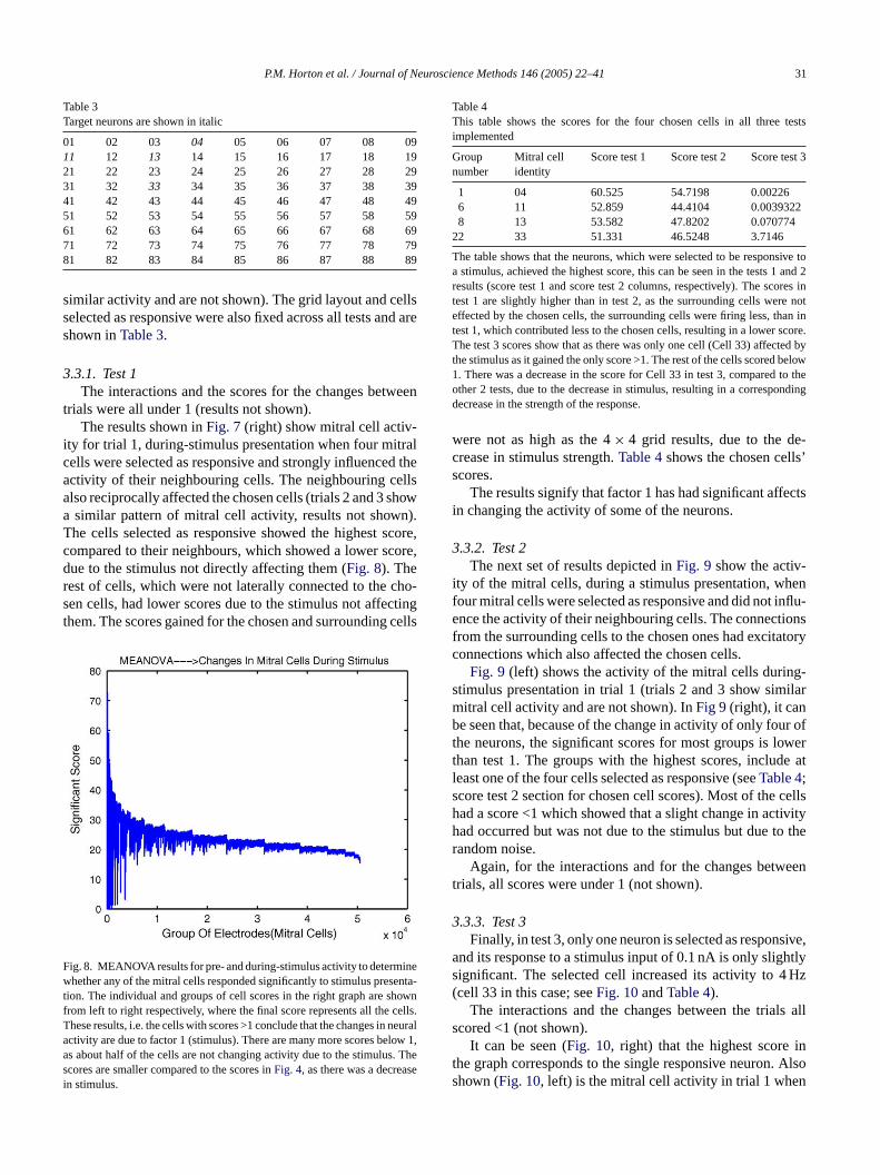
Table 3Target neurons are shown in italic

01 02 03 04 05 06 07 08 0911 12 13 14 15 16 17 18 1921 22 23 24 25 26 27 28 2931 32 33 34 35 36 37 38 3941 42 43 44 45 46 47 48 4951 52 53 54 55 56 57 58 5961 62 63 64 65 66 67 68 6971 72 73 74 75 76 77 78 7981 82 83 84 85 86 87 88 89

similar activity and are not shown). The grid layout and cellsselected as responsive were also fixed across all tests and areshown inTable 3.

3.3.1. Test 1The interactions and the scores for the changes between

trials were all under 1 (results not shown).The results shown inFig. 7(right) show mitral cell activ-

ity for trial 1, during-stimulus presentation when four mitralcells were selected as responsive and strongly influenced theactivity of their neighbouring cells. The neighbouring cellsalso reciprocally affected the chosen cells (trials 2 and 3 showa similar pattern of mitral cell activity, results not shown).The cells selected as responsive showed the highest score,compared to their neighbours, which showed a lower score,due to the stimulus not directly affecting them (Fig. 8). Therest of cells, which were not laterally connected to the cho-sen cells, had lower scores due to the stimulus not affectingthem. The scores gained for the chosen and surrounding cells

F inew enta-t hownf cells.T neuraa low 1,a . Thes sei

Table 4This table shows the scores for the four chosen cells in all three testsimplemented

Groupnumber

Mitral cellidentity

Score test 1 Score test 2 Score test 3

1 04 60.525 54.7198 0.002266 11 52.859 44.4104 0.00393228 13 53.582 47.8202 0.070774

22 33 51.331 46.5248 3.7146

The table shows that the neurons, which were selected to be responsive toa stimulus, achieved the highest score, this can be seen in the tests 1 and 2results (score test 1 and score test 2 columns, respectively). The scores intest 1 are slightly higher than in test 2, as the surrounding cells were noteffected by the chosen cells, the surrounding cells were firing less, than intest 1, which contributed less to the chosen cells, resulting in a lower score.The test 3 scores show that as there was only one cell (Cell 33) affected bythe stimulus as it gained the only score >1. The rest of the cells scored below1. There was a decrease in the score for Cell 33 in test 3, compared to theother 2 tests, due to the decrease in stimulus, resulting in a correspondingdecrease in the strength of the response.

were not as high as the 4× 4 grid results, due to the de-crease in stimulus strength.Table 4shows the chosen cells’scores.

The results signify that factor 1 has had significant affectsin changing the activity of some of the neurons.

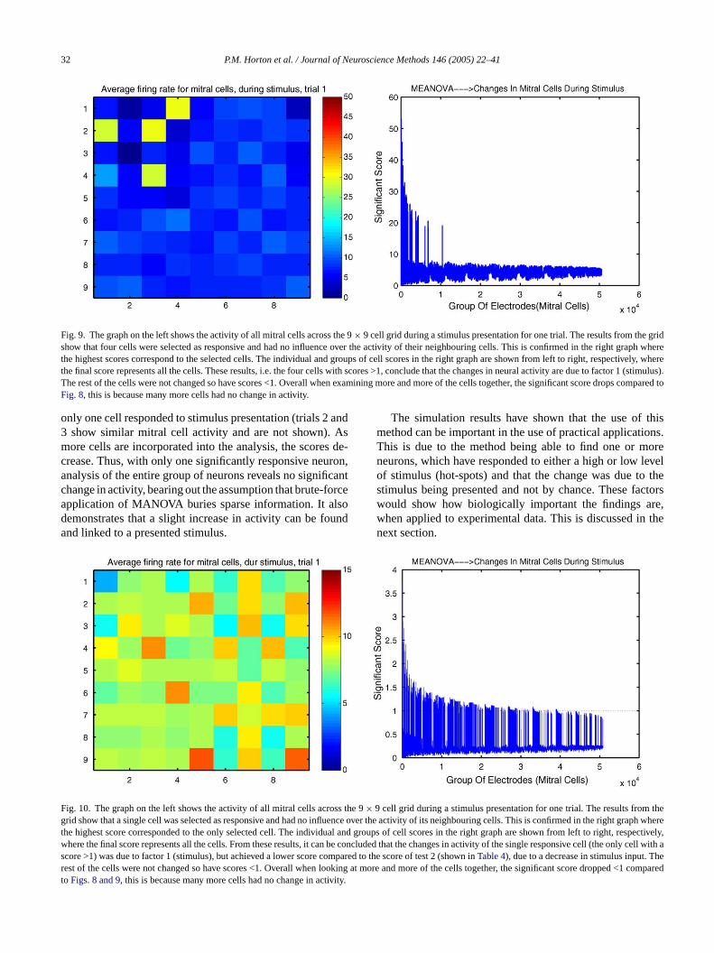
3.3.2. Test 2The next set of results depicted inFig. 9 show the activ-

ity of the mitral cells, during a stimulus presentation, whenfour mitral cells were selected as responsive and did not influ-ence the activity of their neighbouring cells. The connectionsfrom the surrounding cells to the chosen ones had excitatoryconnections which also affected the chosen cells.

Fig. 9 (left) shows the activity of the mitral cells during-stimulus presentation in trial 1 (trials 2 and 3 show similarmitral cell activity and are not shown). InFig 9(right), it canbe seen that, because of the change in activity of only four ofthe neurons, the significant scores for most groups is lowerthan test 1. The groups with the highest scores, include atleast one of the four cells selected as responsive (seeTable 4;score test 2 section for chosen cell scores). Most of the cellshad a score <1 which showed that a slight change in activityhad occurred but was not due to the stimulus but due to therandom noise.

Again, for the interactions and for the changes betweent

3sive,

a htlys Hz(

ls alls

int . Alsos n

ig. 8. MEANOVA results for pre- and during-stimulus activity to determhether any of the mitral cells responded significantly to stimulus pres

ion. The individual and groups of cell scores in the right graph are srom left to right respectively, where the final score represents all thehese results, i.e. the cells with scores >1 conclude that the changes inctivity are due to factor 1 (stimulus). There are many more scores bes about half of the cells are not changing activity due to the stimuluscores are smaller compared to the scores inFig. 4, as there was a decrean stimulus.

l

rials, all scores were under 1 (not shown).

.3.3. Test 3Finally, in test 3, only one neuron is selected as respon

nd its response to a stimulus input of 0.1 nA is only sligignificant. The selected cell increased its activity to 4cell 33 in this case; seeFig. 10andTable 4).

The interactions and the changes between the triacored <1 (not shown).

It can be seen (Fig. 10, right) that the highest scorehe graph corresponds to the single responsive neuronhown (Fig. 10, left) is the mitral cell activity in trial 1 whe

32 P.M. Horton et al. / Journal of Neuroscience Methods 146 (2005) 22–41

Fig. 9. The graph on the left shows the activity of all mitral cells across the 9× 9 cell grid during a stimulus presentation for one trial. The results from the gridshow that four cells were selected as responsive and had no influence over the activity of their neighbouring cells. This is confirmed in the right graph wherethe highest scores correspond to the selected cells. The individual and groups of cell scores in the right graph are shown from left to right, respectively, wherethe final score represents all the cells. These results, i.e. the four cells with scores >1, conclude that the changes in neural activity are due to factor 1 (stimulus).The rest of the cells were not changed so have scores <1. Overall when examining more and more of the cells together, the significant score drops comparedtoFig. 8, this is because many more cells had no change in activity.

only one cell responded to stimulus presentation (trials 2 and3 show similar mitral cell activity and are not shown). Asmore cells are incorporated into the analysis, the scores de-crease. Thus, with only one significantly responsive neuron,analysis of the entire group of neurons reveals no significantchange in activity, bearing out the assumption that brute-forceapplication of MANOVA buries sparse information. It alsodemonstrates that a slight increase in activity can be foundand linked to a presented stimulus.

The simulation results have shown that the use of thismethod can be important in the use of practical applications.This is due to the method being able to find one or moreneurons, which have responded to either a high or low levelof stimulus (hot-spots) and that the change was due to thestimulus being presented and not by chance. These factorswould show how biologically important the findings are,when applied to experimental data. This is discussed in thenext section.

F ss the× 9 theg uence grat al and espew be co ns ompare her oking <1 comparet ivity.

ig. 10. The graph on the left shows the activity of all mitral cells acrorid show that a single cell was selected as responsive and had no infl

he highest score corresponded to the only selected cell. The individuhere the final score represents all the cells. From these results, it cancore >1) was due to factor 1 (stimulus), but achieved a lower score cest of the cells were not changed so have scores <1. Overall when loo Figs. 8 and 9, this is because many more cells had no change in act

9cell grid during a stimulus presentation for one trial. The results fromover the activity of its neighbouring cells. This is confirmed in the rightph wheregroups of cell scores in the right graph are shown from left to right, rctively,

ncluded that the changes in activity of the single responsive cell (the oly cell with ad to the score of test 2 (shown inTable 4), due to a decrease in stimulus input. T

at more and more of the cells together, the significant score droppedd

P.M. Horton et al. / Journal of Neuroscience Methods 146 (2005) 22–41 33

4. Application to recordings from rat olfactory bulb

4.1. The olfactory bulb

The OB is probably the simplest system to be exploredin addressing the issue presented at the start of this paper(Kendrick et al., 1997; Uchida and Mainen, 2003). In themammalian olfactory system, much encoding of odour in-formation takes place in the OB (Desmaisons et al., 1999;Bracci et al., 2003; Debarbieux et al., 2003; Egger et al., 2003;Neville and Haberly, 2003; Pinato and Midtgaard, 2003).Olfactory receptor neurons project to glomeruli in the OB,where they synapse with efferent mitral cells. The quality ofa particular odour is believed to be encoded in the specificcombination of glomeruli activated by that stimulus.

By using MEANOVA to analyse neuronal activity cap-tured using an MEA in the olfactory bulb of the anaesthetisedrat, we hope to find an area (hot-spot) or areas of neuronswhich respond significantly to a stimulus (odour). Questionsthat can be answered from the analysis are whether the stim-ulus is encoded spatially in small groups, i.e. in few neurons,or whether it is encoded in a much larger area where manyneurons are being used for the encoding process. It will alsobe possible to see, due to the sequential trials, if the neuronsrespond to a repeatedly presented stimulus and what affectsit has on the neural activity. Examining the results createdf iono reaw

Before a MEANOVA analysis can be performed on thedata from the rat olfactory bulb, the MEA data must first besorted. Each electrode samples a continuous neural trace, butspiking is detected, and activity is captured when the voltageincreases above a certain threshold. The spikes captured fromeach electrode are grouped according to their waveform char-acteristics (more details on this process will be presented ina forthcoming paper). As the recordings are affected by ex-traneous noise, we try to group the waveforms which havesimilar characteristics. This process results in the number (P)of individual neurons being identified and associated to eachelectrode, where each neuron has a number of action poten-tials (spikes) associated with them.

As discussed in the simulation section, the recording timeand the width of the time bins are problems when analysingneural activity. These need to be chosen wisely, so that wecan obtain and interpret accurate scores from the meanovaprocess. Details of these parameters and the experiment areas follows.

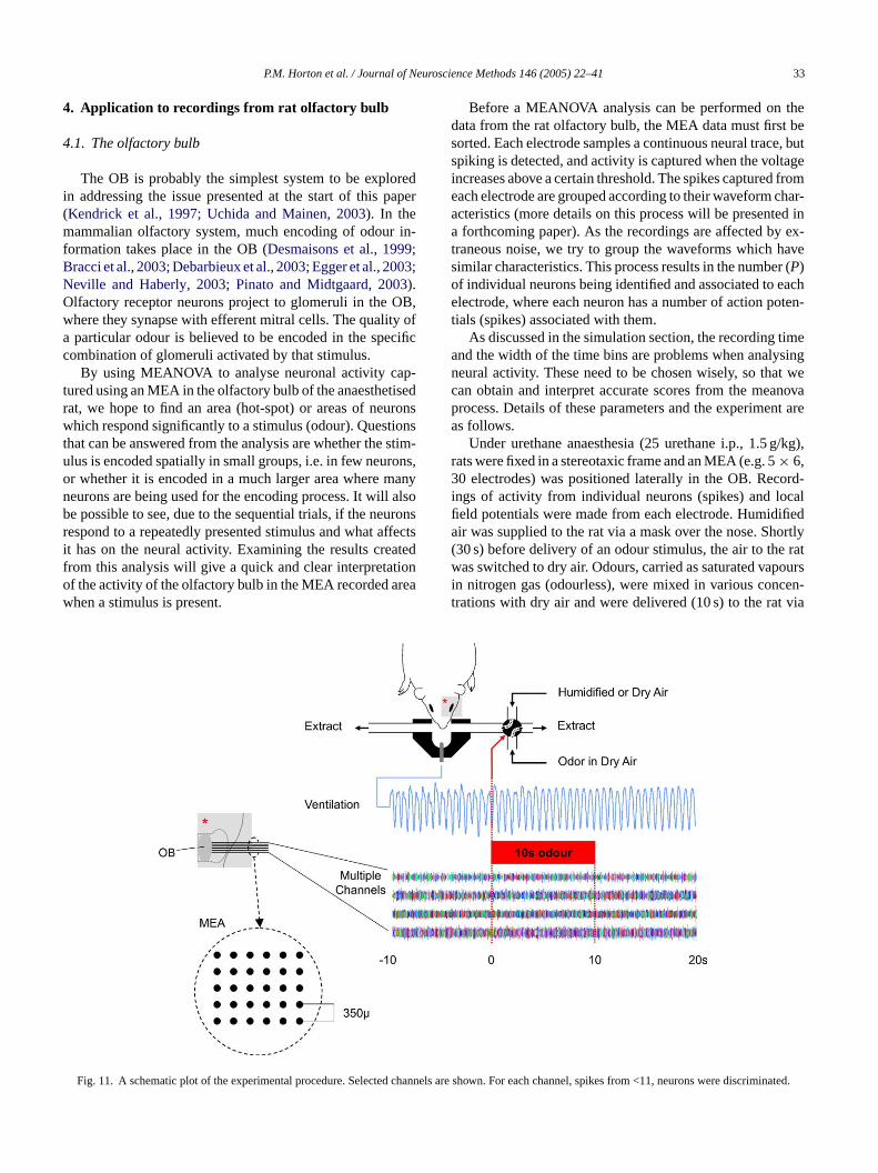
Under urethane anaesthesia (25 urethane i.p., 1.5 g/kg),rats were fixed in a stereotaxic frame and an MEA (e.g. 5× 6,30 electrodes) was positioned laterally in the OB. Record-ings of activity from individual neurons (spikes) and localfield potentials were made from each electrode. Humidifiedair was supplied to the rat via a mask over the nose. Shortly(30 s) before delivery of an odour stimulus, the air to the ratw poursi cen-t via

rom this analysis will give a quick and clear interpretatf the activity of the olfactory bulb in the MEA recorded ahen a stimulus is present.

Fig. 11. A schematic plot of the experimental procedure. Selected channe

as switched to dry air. Odours, carried as saturated van nitrogen gas (odourless), were mixed in various conrations with dry air and were delivered (10 s) to the rat

ls are shown. For each channel, spikes from <11, neurons were discriminated.

34 P.M. Horton et al. / Journal of Neuroscience Methods 146 (2005) 22–41

the mask; three presentations were made of each odour ateach concentration, with an inter-trial interval of≥3 min.Breathing was monitored and onset of odour delivery wasprecisely timed to mid-exhalation (seeFig. 11). Thus, de-livery of the odour to the nasal epithelia would have com-menced from the start of the subsequent inhalation(Nicol etal., 2003).

In our analysis below, we taket = 200 ms and thereare M = T/t = 25 windows for each cell. We also testall results fort = 400 ms and the results are presented inhttp://www.sussex.ac.uk/Users/pmh20. It is noted that thereare no significant changes betweent = 200 and 400 ms.

4.2. Results

In accordance with MEANOVA, we can compare neuronalactivity with many factors: trials, odours, concentration, etc.,as developed in our software. However, here we exclusivelyconsider two factors: factor 1, pre- and during stimulus, andfactor 2, different trials.

4.2.1. RepresentationsThe first difficulty we encounter is the representation prob-

lem. Assume we have a two-dimensional array of electrodesenumerated according to{i, i = 1, . . . ,Q} = Q.

Let us first estimate whether this is possible for an array ofelectrodes. Assume that neuronal activity has been sampledfrom every electrode in the array. Each electrode in the arrayhas four neighbours, and hence, in total we have

Total number of groups> 3√Q

Therefore, the number of groups we have to calculate in-creases exponentially with the total number of electrodes.

In our recordings, we find that electrodes which sampleneuronal activity are usually sparse, but the number maynonetheless be high. In the next section of MEANOVA anal-ysis, we simply map a group of electrodes to a single digitalnumber, as shown inAppendix A. The total number of neigh-bouring electrodes is 286, comparable with 3

√30.

Fad

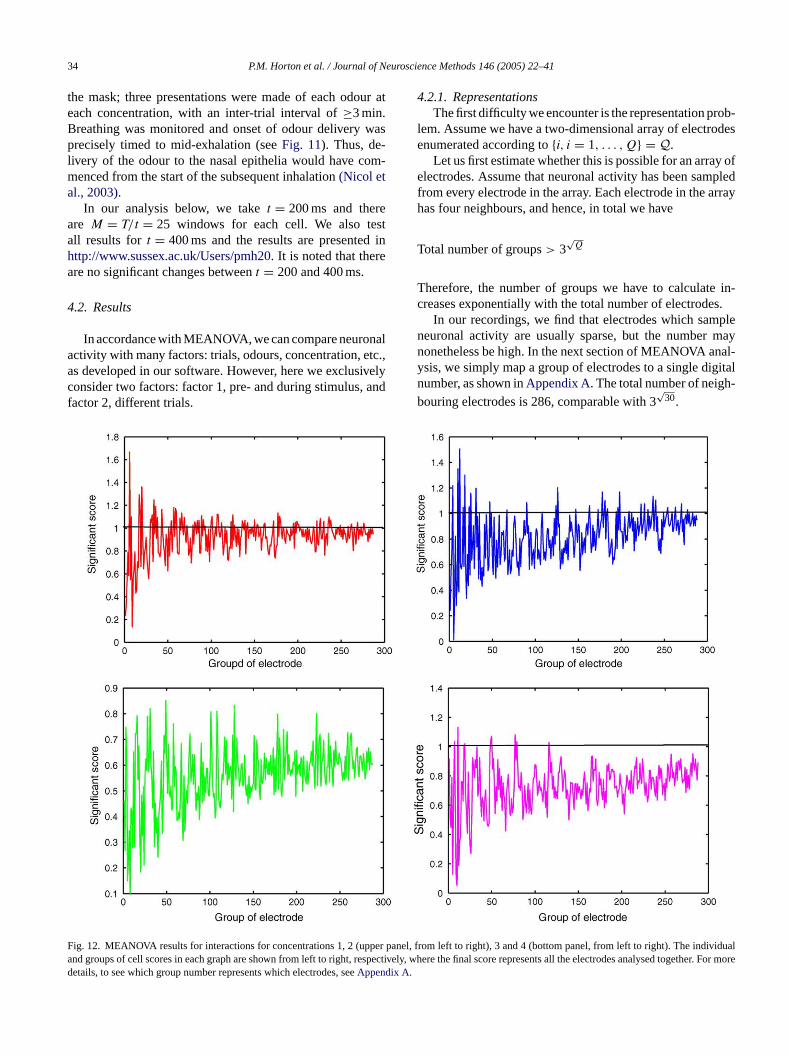
ig. 12. MEANOVA results for interactions for concentrations 1, 2 (upper pand groups of cell scores in each graph are shown from left to right, respectivetails, to see which group number represents which electrodes, seeAppendix A.

nel, from left to right), 3 and 4 (bottom panel, from left to right). The individualely, where the final score represents all the electrodes analysed together. For more

P.M. Horton et al. / Journal of Neuroscience Methods 146 (2005) 22–41 35

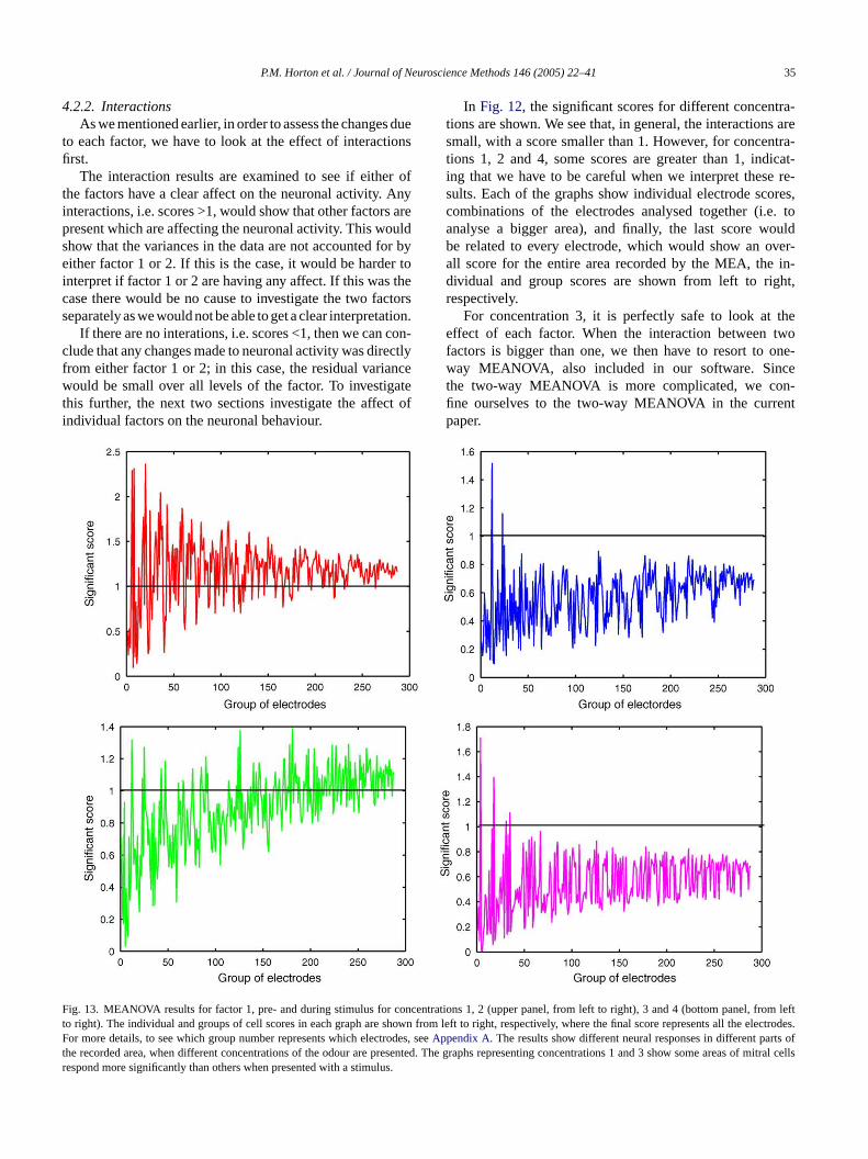
4.2.2. InteractionsAs we mentioned earlier, in order to assess the changes due

to each factor, we have to look at the effect of interactionsfirst.

The interaction results are examined to see if either ofthe factors have a clear affect on the neuronal activity. Anyinteractions, i.e. scores >1, would show that other factors arepresent which are affecting the neuronal activity. This wouldshow that the variances in the data are not accounted for byeither factor 1 or 2. If this is the case, it would be harder tointerpret if factor 1 or 2 are having any affect. If this was thecase there would be no cause to investigate the two factorsseparately as we would not be able to get a clear interpretation.

If there are no interations, i.e. scores <1, then we can con-clude that any changes made to neuronal activity was directlyfrom either factor 1 or 2; in this case, the residual variancewould be small over all levels of the factor. To investigatethis further, the next two sections investigate the affect ofindividual factors on the neuronal behaviour.

In Fig. 12, the significant scores for different concentra-tions are shown. We see that, in general, the interactions aresmall, with a score smaller than 1. However, for concentra-tions 1, 2 and 4, some scores are greater than 1, indicat-ing that we have to be careful when we interpret these re-sults. Each of the graphs show individual electrode scores,combinations of the electrodes analysed together (i.e. toanalyse a bigger area), and finally, the last score wouldbe related to every electrode, which would show an over-all score for the entire area recorded by the MEA, the in-dividual and group scores are shown from left to right,respectively.

For concentration 3, it is perfectly safe to look at theeffect of each factor. When the interaction between twofactors is bigger than one, we then have to resort to one-way MEANOVA, also included in our software. Sincethe two-way MEANOVA is more complicated, we con-fine ourselves to the two-way MEANOVA in the currentpaper.

FtFtr

ig. 13. MEANOVA results for factor 1, pre- and during stimulus for conceno right). The individual and groups of cell scores in each graph are shown for more details, to see which group number represents which electrodes,App

he recorded area, when different concentrations of the odour are presenteespond more significantly than others when presented with a stimulus.

trations 1, 2 (upper panel, from left to right), 3 and 4 (bottom panel, from leftrom left to right, respectively, where the final score represents all the electrodes.seeendix A. The results show different neural responses in different parts ofd. The graphs representing concentrations 1 and 3 show some areas of mitralcells

36 P.M. Horton et al. / Journal of Neuroscience Methods 146 (2005) 22–41

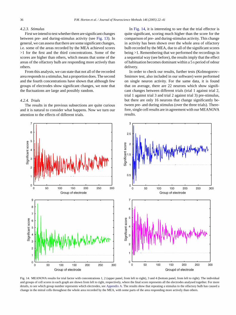
4.2.3. StimulusFirst we intend to test whether there are significant changes

between pre- and during-stimulus activity (seeFig. 13). Ingeneral, we can assess that there are some significant changes,i.e. some of the areas recorded by the MEA achieved scores>1 for the first and the third concentrations. Some of thescores are higher than others, which means that some of theareas of the olfactory bulb are responding more actively thanothers.

From this analysis, we can state that not all of the recordedarea responds to a stimulus, but a proportion does. The secondand the fourth concentrations have shown that although fewgroups of electrodes show significant changes, we note thatthe fluctuations are large and possibly random.

4.2.4. TrialsThe results in the previous subsections are quite curious

and it is natural to consider what happens. Now we turn ourattention to the effects of different trials.

In Fig. 14, it is interesting to see that the trial effector isquite significant, scoring much higher than the score for thecomparison of pre- and during-stimulus activity. This changein activity has been shown over the whole area of olfactorybulb recorded by the MEA, due to all of the significant scoresbeing >1. Remembering that we performed the recordings ina sequential way (see before), the results imply that the effectof habituation becomes dominant within a 5 s period of odourdelivery.

In order to check our results, further tests (Kolmogorov–Smirnov test, also included in our software) were performedon single neuron activity. For the same data, it is foundthat on average, there are 22 neurons which show signifi-cant changes between different trials (trial 1 against trial 2,trial 1 against trial 3 and trial 2 against trial 3) pre-stimulus,but there are only 16 neurons that change significantly be-tween pre- and during stimulus (over the three trials). There-fore, single cell results are in agreement with our MEANOVAresults.

Fadc

ig. 14. MEANOVA results for trial factor with concentrations 1, 2 (upper pannd groups of cell scores in each graph are shown from left to right, respectivetails, to see which group number represents which electrodes, seeAppendix A. Thange in the mitral cells throughout the whole area recorded by the MEA, w

el, from left to right), 3 and 4 (bottom panel, from left to right). The individualely, where the final score represents all the electrodes analysed together. For morehe results show that repeating a stimulus to the olfactory bulb has caused aith some parts of the area responding more actively than others.

P.M. Horton et al. / Journal of Neuroscience Methods 146 (2005) 22–41 37

4.2.5. FluctuationsIt is interesting to note that the magnitudes of fluctuation

of the significant score decrease as|S| increases. In otherwords, with a large value for|S|, the obtained results aremore reliable. Hence, it is natural to ask whether the observedphenomena in the previous subsections are general, or dependon our specific data. InAppendix C, we show theoreticallythat this should be the case.

5. Discussion

We have presented a novel method for applying MANOVAto the analysis of electrophysiological data using a multi-electrode array. By applying this method (MEANOVA) toboth biological and simulated data, we conclude that thisnovel approach is useful for detecting the areas within thearray that are most significantly responsive to external stim-ulation.

The score details the difference in the activity of a clusterof neurons, and if compared with the other scores, provides aninsight into whether the level of change throughout the arearecorded by the MEA is different. In addition to this, the scorealso provides a confidence level that the change in neuralactivity was due to one of the factors under investigation andnot just by chance.

thatM en tablei yedi uites (seeA ea

thatM ofa sam-p thatM ero er ofo bothi toa tiona

oneo atione larges uchs rdingf talr inga

clu-s ech-n lud-i g

(Todd and Marois, 2004) where, again, effects may be sparseacross a large sample of loci.

Acknowledgement

Partially supported by grants from EPSRC(EP/C51338X), (GR/S20574), (GR/S40443) and theRoyal Society (J.F.).

Appendix A

Numbers inside (·) are electrode numbers (seeFig. 1).Digital numbers on the left hand side of an equality representx-axis inFig. 13, with concentration 1.

A.1. Groups attained from real data

1 = (05), 2 = (13), 3 = (15), 4 = (16), 5 = (25), 6 = (26),7 = (35), 8 = (36), 9 = (41), 10 = (43), 11 = (44), 12 = (45),13 = 46 14 = (05 15), 15 = (15 16), 16 = (15 25), 17 = (1626), 18 = (25 26), 19 = (25 35), 20 = (26 36), 21 = (35 36),22 = (43 44), 23 = (35 45), 24 = (44 45), 25 = (36 46), 26 =(45 46), 27 = (05 15 16), 28 = (05 15 25), 29 = (15 16 25),30 = (15 16 26), 31 = (15 25 26), 32 = (16 25 26), 33 = (152 , 37= 444 4 =( 162 253 353 263 263 444 444 354 364 454 151 , 80= 263 5 =( 444 (353 45),9 253 , 98= 162 103= 353 108= 354 113= 162 5 35

From the perspective of methodology, we can sayEANOVA is a valuable extension of MANOVA. As thumber of electrodes increase, the variation becomes s

.e. a more reliable result is obtained. The MEA emplon acquiring the biological data presented here was qmall; neuronal activity was recorded from 11 electrodesppendix A). However, even with relatviely small MEA, wchieve near stablility in the results.

Analysis of simulated data also demonstratedEANOVA yields useful results irrespective of the sizerray used. Whilst only 11 electrodes were used tole the biological data , the simulation demonstratesEANOVA is equally effective with a much larger numbf electrodes. Furthermore, we establish that the numbbservations (time bins) and duration of sampling, are

mportant factors. For example, application of MEANOVAshort period of recording, can yield inaccurate informabout the true character of the data.

It should be emphasised that MEANOVA can detectr several cells responding strongly to stimulus presentven when this responsiveness is embedded within aample of unresponsive cells. MANOVA would hide sparse yet highly significant change. Hence when recorom a large array of electrodes, MEANOVA will play a viole in highlighting hot-spots of activity across the recordrea.

Finally, we want to emphasize that although we exively discuss our approach for dealing MEA data, this tique is readily applicable to many other types of data inc

ng gene microarrays(Riemer et al., 2004)and brain imagin

,

5 35), 34 = (16 26 36), 35 = (25 26 35), 36 = (25 26 36)(25 35 36), 38 = (26 35 36), 39 = (25 35 45), 40 = (35

5), 41 = (35 45 46), 42 = (43 44 45), 43 = (26 36 46), 435 36 45), 45 = (35 36 46), 46 = (44 45 46), 47 = (05 155), 48 = (05 15 16 26), 49 = (05 15 25 26), 50 = (05 155), 51 = (15 16 25 26), 52 = (15 16 25 35), 53 = (15 256), 54 = (16 26 35 36), 55 = (15 25 35 45), 56 = (16 255), 57 = (15 16 26 36), 58 = (15 25 26 35), 59 = (15 256), 60 = (16 25 26 36), 61 = (25 35 44 45), 62 = (35 435), 63 = (25 35 45 46), 64 = (26 35 36 45), 65 = (35 365), 66 = (16 26 36 46), 67 = (25 26 35 36), 68 = (25 265), 69 = (25 26 36 46), 70 = (25 35 36 45), 71 = (25 356), 72 = (26 35 36 46), 73 = (35 36 45 46), 74 = (35 446), 75 = (43 44 45 46), 76 = (05 15 16 25 26), 77 = (056 25 35), 78 = (05 15 25 26 35), 79 = (05 15 25 26 36)(05 15 25 35 36), 81 = (15 16 26 35 36), 82 = (15 25

5 36), 83 = (16 25 26 35 45), 84 = (16 26 35 36 45), 825 35 36 44 45), 86 = (26 35 36 44 45), 87 = (25 35 435), 88 = (25 35 44 45 46), 89 = (26 36 44 45 46), 90 =6 43 44 45), 91 = (16 25 26 36 46), 92 = (15 25 35 363 = (16 26 35 36 46), 94 = (15 25 35 44 45), 95 = (155 36 46), 96 = (15 25 35 45 46), 97 = (16 25 26 35 36)(05 15 25 35 45), 99 = (15 16 25 26 35), 100 = (05 15

6 36), 101 = (15 16 25 26 36), 102 = (15 16 25 35 36),(15 16 25 35 45), 104 = (15 25 26 35 45), 105 = (25 266 45), 106 = (25 26 35 44 45), 107 = (15 16 26 36 46),(15 25 26 36 46), 109 = (25 26 35 36 46), 110 = (25 265 46), 111 = (25 35 36 45 46), 112 = (26 35 36 45 46),(35 36 44 45 46), 114 = (35 43 44 45 46), 115 = (05 155 26 35), 116 = (05 15 16 25 26 36), 117 = (05 15 16 2

38 P.M. Horton et al. / Journal of Neuroscience Methods 146 (2005) 22–41

36), 118 = (05 15 16 26 35 36), 119 = (05 15 25 35 44 45),120 = (05 15 25 35 45 46), 121 = (15 16 25 35 44 45), 122= (15 16 25 35 45 46), 123 = (16 26 35 36 44 45), 124 = (1525 35 43 44 45), 125 = (16 26 36 44 45 46), 126 = (25 26 3543 44 45), 127 = (05 15 16 26 36 46), 128 = (05 15 25 26 3536), 129 = (05 15 25 26 35 45), 130 = (05 15 25 26 36 46),131 = (05 15 25 35 36 46), 132 = (15 16 25 26 35 36), 133= (05 15 16 25 35 45), 134 = (15 16 25 26 35 45), 135 = (1516 25 35 36 46), 136 = (15 16 26 35 36 45), 137 = (15 25 2635 36 45), 138 = (15 25 35 36 44 45), 139 = (25 26 36 44 4546), 140 = (25 35 43 44 45 46), 141 = (26 35 36 43 44 45),142 = (16 26 35 36 45 46), 143 = (25 35 36 43 44 45), 144= (15 25 35 36 45 46), 145 = (16 25 26 35 36 45), 146 = (1625 26 35 44 45), 147 = (25 26 35 36 44 45), 148 = (16 25 2635 36 46), 149 = (15 25 26 35 44 45), 150 = (15 16 25 26 3646), 151 = (05 15 25 35 36 45), 152 = (15 16 25 35 36 45),153 = (15 16 26 35 36 46), 154 = (15 25 26 35 36 46), 155= (15 25 26 35 45 46), 156 = (16 25 26 35 45 46), 157 = (2526 35 36 45 46), 158 = (15 25 35 44 45 46), 159 = (25 26 3544 45 46), 160 = (25 35 36 44 45 46), 161 = (26 35 36 44 4546), 162 = (26 36 43 44 45 46), 163 = (35 36 43 44 45 46),164 = (05 15 16 25 26 35 36), 165 = (05 15 16 25 26 35 45),166 = (05 15 16 25 35 44 45), 167 = (05 15 16 25 35 45 46),168 = (05 15 25 26 35 44 45), 169 = (05 15 25 26 35 45 46),170 = (05 15 25 35 36 44 45), 171 = (15 16 25 35 36 44 45),172 = (15 16 26 35 36 44 45), 173 = (05 15 25 35 43 44 45),1 45),1 46),1 46),1 45),1 45),1 45),1 45),1 45),1 46),1 45),1 46),1 46),1 46),2 46),2 45),2 46),2 46),2 46),2 46),2 46),2 6 354 6 253 5 152 21 =( 46),2 5 444 5 263 5 152 30 =( 46),

232 = (15 16 25 26 35 43 44 45), 233 = (15 16 25 35 36 4344 45), 234 = (15 16 25 35 43 44 45 46), 235 = (15 16 26 3536 43 44 45), 236 = (15 16 26 36 43 44 45 46), 237 = (15 2526 35 36 43 44 45), 238 = (15 25 26 36 43 44 45 46), 239 =(16 25 26 36 43 44 45 46), 240 = (15 25 35 36 43 44 45 46),241 = (16 25 26 35 36 43 44 45), 242 = (05 15 16 25 26 3536 46), 243 = (05 15 16 25 35 36 45 46), 244 = (05 15 16 2635 36 45 46), 245 = (05 15 25 26 35 36 45 46), 246 = (15 1625 26 35 36 44 45), 247 = (15 16 25 26 35 36 45 46), 248 =(15 16 25 26 35 44 45 46), 249 = (15 25 26 35 36 44 45 46),250 = (15 25 26 35 43 44 45 46), 251 = (16 25 26 35 36 4445 46), 252 = (16 25 26 35 43 44 45 46), 253 = (16 26 35 3643 44 45 46), 254 = (25 26 35 36 43 44 45 46), 255 = (05 1516 25 26 35 36 44 45), 256 = (05 15 16 25 26 35 43 44 45),257 = (05 15 16 25 26 35 44 45 46), 258 = (05 15 16 25 2636 44 45 46), 259 = (05 15 16 25 35 36 43 44 45), 260 = (0515 16 25 35 36 44 45 46), 261 = (05 15 16 26 35 36 44 4546), 262 = (05 15 16 26 36 43 44 45 46), 263 = (05 15 25 2635 36 44 45 46), 264 = (05 15 16 25 35 43 44 45 46), 265 =(05 15 16 26 35 36 43 44 45), 266 = (05 15 25 26 35 36 4344 45), 267 = (05 15 25 26 35 43 44 45 46), 268 = (05 15 2526 36 43 44 45 46), 269 = (15 16 25 26 36 43 44 45 46), 270= (05 15 25 35 36 43 44 45 46), 271 = (15 16 25 26 35 36 4344 45), 272 = (05 15 16 25 26 35 36 45 46), 273 = (15 16 2526 35 36 44 45 46), 274 = (15 16 25 26 35 43 44 45 46), 275= (15 16 25 35 36 43 44 45 46), 276 = (15 16 26 35 36 43 444 5 263 45),2 6 252 46),2 6 263 46),2 6 252

A

B

= 13= (031 3),2 , 26= 041 3 =( 24),3 (232 112 212 112 041 222 222 02

74 = (05 15 25 35 44 45 46), 175 = (15 16 25 35 43 4476 = (15 16 25 35 44 45 46), 177 = (15 16 26 36 44 4578 = (15 25 26 35 43 44 45), 179 = (15 25 26 36 44 4580 = (16 25 26 36 44 45 46), 181 = (15 25 35 36 43 4482 = (16 25 26 35 43 44 45), 183 = (16 26 35 36 43 4484 = (05 15 16 25 26 36 46), 185 = (05 15 16 25 35 3686 = (05 15 16 25 35 36 46), 187 = (05 15 16 26 35 3688 = (05 15 16 26 35 36 46), 189 = (05 15 25 26 35 3690 = (05 15 25 26 35 36 46), 191 = (05 15 25 35 36 4592 = (15 16 25 26 35 36 45), 193 = (15 16 25 26 35 4494 = (15 16 25 35 36 45 46), 195 = (16 26 35 36 44 4596 = (15 25 35 43 44 45 46), 197 = (16 26 36 43 44 4598 = (25 26 35 36 43 44 45), 199 = (15 16 26 35 36 4500 = (15 25 26 35 36 44 45), 201 = (15 25 26 35 36 4502 = (15 25 35 36 44 45 46), 203 = (16 25 26 35 36 4404 = (15 16 25 26 35 36 46), 205 = (15 16 25 26 35 4506 = (16 25 26 35 36 45 46), 207 = (15 25 26 35 44 4508 = (16 25 26 35 44 45 46), 209 = (25 26 35 36 44 4510 = (25 26 35 43 44 45 46), 211 = (25 26 36 43 44 4512 = (25 35 36 43 44 45 46), 213 = (26 35 36 43 44 4514 = (05 15 16 25 26 35 36 45), 215 = (05 15 16 25 24 45), 216 = (05 15 16 25 26 35 45 46), 217 = (05 15 15 36 44 45), 218 = (05 15 16 26 35 36 44 45), 219 = (05 26 35 36 44 45), 220 = (05 15 16 25 35 43 44 45), 205 15 16 25 35 44 45 46), 222 = (05 15 16 26 36 44 4523 = (05 15 25 26 35 43 44 45), 224 = (05 15 25 26 35 46), 225 = (05 15 25 26 36 44 45 46), 226 = (15 16 26 44 45 46), 227 = (05 15 25 35 36 43 44 45), 228 = (05 35 36 44 45 46), 229 = (15 16 25 35 36 44 45 46), 215 16 26 35 36 44 45 46), 231 = (05 15 25 35 43 44 45

5 46), 277 = (15 25 26 35 36 43 44 45 46), 278 = (16 25 36 43 44 45 46), 279 = (05 15 16 25 26 35 36 43 4480 = (05 15 16 25 26 35 36 44 45 46), 281 = (05 15 16 35 43 44 45 46), 282 = (05 15 16 25 26 36 43 44 4583 = (05 15 16 25 35 36 43 44 45 46), 284 = (05 15 15 36 43 44 45 46), 285 = (05 15 25 26 35 36 43 44 4586 = (15 16 25 26 35 36 43 44 45 46), 287 = (05 15 16 35 36 43 44 45 46), =Q.

ppendix B

.1. Groups attained from simulated data

1 = (01), 2 = (02), 3 = (03), 4 = (04), 5 = (11), 6 = (13), 7(21), 8 = (22), 9 = (23), 10 = (24), 11 = (31), 12 = (33),(01 02), 14 = (01 11), 15 = (02 03), 16 = (03 04), 17 =3), 18 = (11 21), 19 = (21 22), 20 = (13 23), 21 = (22 22 = (23 24), 23 = (21 31), 24 = (23 33), 25 = (01 02 03)(01 11 21), 27 = (02 03 04), 28 = (02 03 13), 29 = (03

3), 30 = (11 21 22), 31 = (03 13 23), 32 = (13 22 23), 313 23 24), 34 = (13 23 33), 35 = (21 22 23), 36 = (22 237 = (11 21 31), 38 = (21 22 31), 39 = (22 23 33), 40 =4 33), 41 = (01 02 03 04), 42 = (01 02 03 13), 43 = (011 22), 44 = (03 13 22 23), 45 = (11 21 22 23), 46 = (132 23), 47 = (03 13 23 24), 48 = (21 22 23 24), 49 = (011 31), 50 = (02 03 04 13), 51 = (02 03 13 23), 52 = (033 23), 53 = (21 22 23 31), 54 = (03 13 23 33), 55 = (133 24), 56 = (11 21 22 31), 57 = (13 22 23 33), 58 = (213 33), 59 = (13 23 24 33), 60 = (22 23 24 33), 61 = (01

P.M. Horton et al. / Journal of Neuroscience Methods 146 (2005) 22–41 39

03 04 13), 62 = (01 02 03 11 21), 63 = (01 02 03 13 23), 64= (01 11 21 22 23), 65 = (03 13 21 22 23), 66 = (11 13 2122 23), 67 = (03 13 22 23 24), 68 = (11 21 22 23 24), 69 =(13 21 22 23 24), 70 = (01 11 21 22 31), 71 = (02 03 04 1323), 72 = (02 03 13 22 23), 73 = (03 04 13 22 23), 74 = (0203 13 23 24), 75 = (03 04 13 23 24), 76 = (11 21 22 23 31),77 = (13 21 22 23 31), 78 = (13 21 22 23 33), 79 = (21 22 2324 31), 80 = (02 03 13 23 33), 81 = (03 04 13 23 33), 82 =(03 13 22 23 33), 83 = (11 21 22 23 33), 84 = (03 13 23 2433), 85 = (13 22 23 24 33), 86 = (21 22 23 24 33), 87 = (2122 23 31 33), 88 = (01 02 03 4 11 21), 89 = (01 02 03 11 1321), 90 = (01 02 03 11 21 22), 91 = (01 02 03 04 13 23), 92= (01 02 03 13 22 23), 93 = (01 02 03 13 23 24), 94 = (01 0203 13 23 33), 95 = (01 11 13 21 22 23), 96 = (01 11 21 22 2324), 97 = (01 11 21 22 23 33), 98 = (02 03 13 21 22 23), 99= (03 04 13 21 22 23), 100 = (03 13 21 22 23 24), 101 = (0102 03 11 21 31), 102 = (01 11 21 22 23 31), 103 = (02 03 0413 22 23), 104 = (03 11 13 21 22 23), 105 = (02 03 04 13 2324), 106 = (02 03 13 22 23 24), 107 = (03 04 13 22 23 24),108 = (03 13 21 22 23 31), 109 = (03 13 21 22 23 33), 110= (11 13 21 22 23 24), 111 = (11 13 21 22 23 31), 112 = (1121 22 23 24 31), 113 = (13 21 22 23 24 31), 114 = (02 03 0413 23 33), 115 = (02 03 13 22 23 33), 116 = (03 04 13 22 2333), 117 = (11 13 21 22 23 33), 118 = (02 03 13 23 24 33),119 = (03 04 13 23 24 33), 120 = (03 13 22 23 24 33), 121= (11 21 22 23 24 33), 122 = (13 21 22 23 24 33), 123 = (112 2 232 3 041 3 041 3 112 3 132 3 132 3 212 1 222 1 222 3 212 3 041 3 111 3 112 1 132 3 212 4 132 3 212 3 212 1 222 1 222 3 212 3 222 1 222 2 232 3 041 1 020 77 =( 31),1 3 232 3 04

13 22 23 24), 183 = (01 02 03 04 13 22 23 33), 184 = (01 0203 11 21 22 23 24), 185 = (01 02 03 11 21 22 23 33), 186 =(01 02 03 13 21 22 23 24), 187 = (01 02 03 13 21 22 23 33),188 = (01 03 11 13 21 22 23 33), 189 = (01 02 03 13 22 2324 33), 190 = (01 03 11 13 21 22 23 24), 191 = (01 11 13 2122 23 24 31), 192 = (01 11 13 21 22 23 24 33), 193 = (01 1113 21 22 23 31 33), 194 = (01 11 21 22 23 24 31 33), 195 =(02 03 04 13 21 22 23 24), 196 = (01 02 03 04 11 13 21 31),197 = (01 02 03 04 11 21 22 31), 198 = (01 02 03 11 13 2122 23), 199 = (01 02 03 11 13 21 22 31), 200 = (01 02 03 1113 21 23 31), 201 = (01 02 03 11 21 22 23 31), 202 = (02 0304 13 21 22 23 31), 203 = (02 03 04 13 21 22 23 33), 204 =(01 03 11 13 21 22 23 31), 205 = (02 03 04 11 13 21 22 23),206 = (02 03 11 13 21 22 23 24), 207 = (02 03 11 13 21 2223 31), 208 = (02 03 13 21 22 23 24 31), 209 = (02 03 13 2122 23 24 33), 210 = (03 04 13 21 22 23 24 31), 211 = (03 0413 21 22 23 24 33), 212 = (02 03 13 21 22 23 31 33), 213 =(03 04 11 13 21 22 23 24), 214 = (03 04 11 13 21 22 23 31),215 = (03 04 13 21 22 23 31 33), 216 = (03 11 13 21 22 2324 31), 217 = (02 03 11 13 21 22 23 33), 218 = (03 04 11 1321 22 23 33), 219 = (02 03 04 13 22 23 24 33), 220 = (03 1113 21 22 23 24 33), 221 = (03 11 13 21 22 23 31 33), 222 =(03 13 21 22 23 24 31 33), 223 = (11 13 21 22 23 24 31 33),224 = (01 02 03 04 11 13 21 22 23), 225 = (01 02 03 04 1113 21 23 24), 226 = (01 03 04 11 13 21 22 23 24), 227 = (0102 03 04 13 21 22 23 31), 228 = (01 03 04 11 13 21 22 233 3 132 32 =( 1 232 2 030 237= 1 232 2 030 242= 3 212 2 031 247= 2 233 2 031 252= 2 233 3 041 257= 222 2 031 33),2 1 132 (020 3 243 3 212 70 =( 1 132 73 =( 3 212 76 =( 3 21

1 22 23 31 33), 124 = (13 21 22 23 31 33), 125 = (21 24 31 33), 126 = (01 02 03 04 11 13 21), 127 = (01 02 01 21 22), 128 = (01 02 03 04 13 22 23), 129 = (01 02 03 23 24), 130 = (01 02 03 04 13 23 33), 131 = (01 02 01 22 23), 132 = (01 02 03 13 21 22 23), 133 = (01 02 02 23 24), 134 = (01 02 03 13 22 23 33), 135 = (01 02 03 24 33), 136 = (01 11 13 21 22 23 24), 137 = (01 11 12 23 31), 138 = (01 11 13 21 22 23 33), 139 = (01 11 23 24 31), 140 = (01 11 21 22 23 24 33), 141 = (01 11 23 31 33), 142 = (02 03 04 13 21 22 23), 143 = (02 03 12 23 24), 144 = (03 04 13 21 22 23 24), 145 = (01 02 01 21 31), 146 = (01 02 03 11 13 21 22), 147 = (01 02 03 21 23), 148 = (01 02 03 11 13 21 31), 149 = (01 02 01 22 31), 150 = (01 03 11 13 21 22 23), 151 = (02 03 11 22 23), 152 = (02 03 13 21 22 23 31), 153 = (02 03 12 23 33), 154 = (03 04 11 13 21 22 23), 155 = (02 03 02 23 24), 156 = (03 04 13 21 22 23 31), 157 = (03 04 12 23 33), 158 = (03 11 13 21 22 23 24), 159 = (03 11 12 23 31), 160 = (03 13 21 22 23 24 31), 161 = (03 13 23 24 33), 162 = (03 13 21 22 23 31 33), 163 = (11 13 23 24 31), 164 = (02 03 04 13 22 23 33), 165 = (03 11 12 23 33), 166 = (02 03 04 13 23 24 33), 167 = (02 03 13 24 33), 168 = (03 04 13 22 23 24 33), 169 = (11 13 23 24 33), 170 = (11 13 21 22 23 31 33), 171 = (11 21 24 31 33), 172 = (13 21 22 23 24 31 33), 173 = (01 02 01 13 21 22), 174 = (01 02 03 04 11 13 21 23), 175 = (03 04 11 21 22 23), 176 = (01 02 03 04 13 21 22 23), 101 03 04 11 13 21 22 23), 178 = (01 02 03 13 21 22 2379 = (01 02 03 11 13 21 23 33), 180 = (01 02 03 04 14 33), 181 = (01 02 03 11 13 21 23 24), 182 = (01 02 0

1), 229 = (01 03 04 11 13 21 22 23 33), 230 = (01 02 01 22 23 24 31), 231 = (01 02 03 04 11 13 21 23 33), 201 02 03 04 11 21 22 23 24), 233 = (01 02 03 11 13 24 31), 234 = (01 02 03 04 11 21 22 23 33), 235 = (01 04 13 21 22 23 24), 236 = (01 02 03 04 13 21 22 23 33),(01 02 03 11 13 21 22 23 33), 238 = (01 02 03 11 13 24 33), 239 = (01 02 03 11 13 21 23 31 33), 240 = (01 04 13 22 23 24 33), 241 = (01 02 03 11 13 21 22 23 24),(01 02 03 04 11 13 21 22 31), 243 = (01 02 03 04 11 13 31), 244 = (01 02 03 04 11 21 22 23 31), 245 = (01 01 13 21 22 23 31), 246 = (01 02 03 11 21 22 23 24 31),(01 02 03 11 21 22 23 24 33), 248 = (01 02 03 11 21 21 33), 249 = (01 02 03 13 21 22 23 24 33), 250 = (01 03 21 22 23 31 33), 251 = (01 03 11 13 21 22 23 24 31),(01 03 11 13 21 22 23 24 33), 253 = (01 03 11 13 21 21 33), 254 = (01 11 13 21 22 23 24 31 33), 255 = (02 01 13 21 22 23 24), 256 = (02 03 04 11 13 21 22 23 31),(02 03 04 13 21 22 23 24 31), 258 = (02 03 04 13 21

3 24 33), 259 = (02 03 04 13 21 22 23 31 33), 260 = (01 13 21 22 23 24 31), 261 = (02 03 13 21 22 23 24 3162 = (03 04 11 13 21 22 23 24 31), 263 = (02 03 04 11 22 23 33), 264 = (02 03 11 13 21 22 23 24 33), 265 =3 11 13 21 22 23 31 33), 266 = (03 04 11 13 21 22 23), 267 = (03 04 11 13 21 22 23 31 33), 268 = (03 04 12 23 24 31 33), 269 = (03 11 13 21 22 23 24 31 33), 201 02 03 04 11 13 21 22 23 24), 271 = (01 02 03 04 11 22 23 31), 272 = (01 02 03 04 11 13 21 23 24 31), 201 02 03 04 13 21 22 23 24 31), 274 = (01 03 04 11 12 23 24 31), 275 = (01 02 03 04 11 13 21 22 23 33), 201 02 03 04 11 13 21 23 24 33), 277 = (01 03 04 11 1

40 P.M. Horton et al. / Journal of Neuroscience Methods 146 (2005) 22–41

22 23 24 33), 278 = (01 02 03 04 11 13 21 23 31 33), 279 =(01 02 03 04 11 21 22 23 24 31), 280 = (01 02 03 04 11 2122 23 24 33), 281 = (01 02 03 04 11 21 22 23 31 33), 282 =(01 02 03 04 13 21 22 23 24 33), 283 = (01 02 03 04 13 2122 23 31 33), 284 = (01 02 03 11 13 21 22 23 24 31), 285 =(01 02 03 11 13 21 22 23 24 33), 286 = (01 02 03 11 13 2122 23 31 33), 287 = (01 03 4 11 13 21 22 23 31 33), 288 =(01 02 03 11 13 21 23 24 31 33), 289 = (01 02 03 11 21 2223 24 31 33), 290 = (01 02 03 13 21 22 23 24 31 33), 291 =(01 03 11 13 21 22 23 24 31 33), 292 = (02 03 04 11 13 2122 23 24 31), 293 = (02 03 04 11 13 21 22 23 24 33), 294 =(02 03 04 11 13 21 22 23 31 33), 295 = (02 03 04 13 21 2223 24 31 33), 296 = (02 03 11 13 21 22 23 24 31 33), 297 =(03 04 11 13 21 22 23 24 31 33), 298 = (01 02 03 04 11 1321 22 23 24 31), 299 = (01 02 03 04 11 13 21 22 23 24 33),300 = (01 02 03 04 11 13 21 22 23 31 33), 301 = (01 02 0304 11 13 21 23 24 31 33), 302 = (01 02 03 04 11 21 22 23 2431 33), 303 = (01 02 03 04 13 21 22 23 24 31 33), 304 = (0102 03 11 13 21 22 23 24 31 33), 305 = (01 03 04 11 13 21 2223 24 31 33), 306 = (02 03 04 11 13 21 22 23 24 31 33), 307= (01 02 03 04 11 13 21 22 23 24 31 33).

Appendix C

ionsw

S

W tw

|

i -s sidert

ma law)( tt si

P

W

|

Hence,

log |Sr||S|

[log λ1 + · · · + logλ|S|]|S| → E logλ1

whereλ1 is distributed according toPSr . We then have

log |Sr|∼|S|E logλ1

Similarly, for the matrixS2 + Sr, we conclude that

log |Sr + S2|∼|S| logEλ̄1

whereλ̄1 is the eigenvalue of the matrixSr + S2.Combining all arguments above, we assert that the limit

exists and so the fluctuation will become smaller and smaller.

References

Albright TD, Jessell TM, Kandel ER, Posner MI. Neural science: a centuryof progress and the mysteries that remain. Cell 2000;100:S1–55.

Bartletts MS. A note on the multiplying factors for variousχ2 approxima-tions. J R Stat Soc 1954;16:294–8.

Bracci E, Centonze D, Bernardi G, Calabresi P. Voltage-dependent mem-brane potential oscillations of rat striatal fast-spiking interneurons. JPhysiol 2003;549:121–30.

B om-Phys

C their

D our-uro-

D athe-

D den-

D ingns. J

E theflux

F ew

F apman

H robab

H Appl

J recordtion.

J h ed.

K em-

M yieldysiol

Here, we want to show theoretically that the fluctuatill become smaller as observed in MEANOVA results.Let us look atS2(S),

2(S) = −∣∣∣∣IJ(M − 1) − |S| + 1 − (J − 1)

2

∣∣∣∣ lnΛ2

χ2(J−1)|S|(α)

e could assume thatIJ(M − 1)/χ2(J−1)|S|(α) is a constan

hen|S| is large. It is easily seen that

limS|→∞

|S|χ2

(J−1)|S|(α)

s a constant. For example, whenJ = 2, α = 0.05, the contant is 1. To assess the existence of limit, we need to conhe limit of Λ2, which is more mathematically involved.

Let us assume thatSr is a random, symmetric matrix. Frogeneral results in random matrix (the Quarter circle

Cohen and Newman, 1984; Brody et al., 1981), we know thahe asymptotic eigenvalue density function ofSr convergen probability to

Sr (x) = 1

2π

√4 − x

x, 0 < x < 4

e know that

Sr| = λ1 . . . λ|S|

rody TA, Flores J, French JB, Mello PA, Pandey A, Wong SSM. Randmatrix physics: spectrum and strength fluctuations. Rev Mod1981;53:385–479.

ohen JE, Newman CM. The stability of large random matrices andproducts. Ann Probability 1984;12:283–310.

avison A, Feng JF, Brown D. Dendrodendritic inhibition and odinduced synchronization in a detailed olfactory bulb model. J Nephysiol 2003;90:192–3.

ayan P, Abbott LF. Theoretical neuroscience: computational and mmatical modeling of neural systems. MIT Press; 2001.

ebarbieux F, Audinat E, Charpak S. Action potential propagation indrites of rate mitral cells in vivo. J Neurosci 2003;23:5553–60.

esmaisons D, Vincent JD, Lledo PM. Control of action potential timby intrinsic subthreshold oscillations in olfactory bulb ouput neuroNeurosci 1999;19:10727–37.

gger V, Svoboda K, Mainen ZF. Mechanisms of lateral inhibition inolfactory bulb: efficiency and modulation of spike-evoked calcium ininto granule cells. J Neurosci 2003;23:7551–8.

eller W. An introduction to probability theory and its application. NYork: John Wiley and Sons; 1971.

eng JF. Computational neuroscience: a comprehensive approach. Chand Hall/CRC Press; 2004.

unter JJ. Renewal theory in two dimensions: basic results. Adv Appl P1974;6:376–91.

unter JJ. Renewal theory in two dimensions: asymptotic results. AdvProbab 1974;6:546–62.

ohnson JL, Welsh JP. Independently movable multielectrode array tomultiple fast-spiking neurons in the cerebral cortex during cogniMethods 2003;30:64–78.

ohnson RA, Wichern DW. Applied multivariate statistical analysis. 4tPrentice Hall; 1988.

endrick KM, GuevaraGuzman R, Zorrilla J. Formation of olfactory mories mediated by nitric oxide. Nature 1997;388:670–4.

argrie T, Schaefer A. Theta osciallation coupled spike latenciescomputational vigour in a mammalian sensory system. J Ph2003;546:363–74.

P.M. Horton et al. / Journal of Neuroscience Methods 146 (2005) 22–41 41

Maynard EM, Hatsopoulos NG, Ojakangas CL, Acuna BD, Sanes JN,Normann RA, Donoghue JP. Neuronal interactions improve corticalpopulation coding of movement direction. J Neurosci 1999;19:8083–93.

Neville KR, Haberly LB. Beta and gamma oscillations in the olfactory systemof the urethane-anesthetized rat. J Neurophysiol 2003;90:3921–30.

Nicol A, Man MS, Feng JF, Mason R, Kendrick K. Differential spatial acti-vation patterns evoled by odor stimui in the rate olfactory bulb. AnnualMeeting of Neuroscience; 2003.

Patterson WR, Song YK, Bull CW, Ozden I, Deangellis AP, Lay C,McKay JL, Nurmikko AV, Donoghue JD, Connors BW. A micro-electrode/microelectronic hybrid device for brain implantable neu-roprosthesis applications. IEEE Trans Biomed Eng 2004;51:1845–53.

Pinato G, Midtgaard J. Regulation of granule cell excitability by alow-threshold calcium spike in turtle olfactory bulb. J Neurophysiol2003;90:3341–51.

Riemer C, Neidhold S, Burwinkel M, Schwarz A, Schultz J, KratzschmarJ, Monning U, Baier M. Gene expression profiling of scrapie-infected brain tissue. Biochem Biophys Res Commun 2004;323:556–64.

Todd JJ, Marois R. Capacity limit of visual short-term memory in humanposterior parietal cortex. Nature 2004;428:751–4.

Uchida N, Mainen ZF. Speed and accuracy of olfactory discrimination in therat. Nat: Neurosci 2003;1224–9.

Warwick K, Gasson M, Hutt B, Goodhew I, Kyberd P, Andrews B, Teddy P,Shad A. The application of implant technology for cybernetic systems.Arch Neurol 2004;60:1369–73.