Embed Size (px)
Citation preview
Applications of machine learning in speech and audio processing
Amir R. Moghimi
July 2020
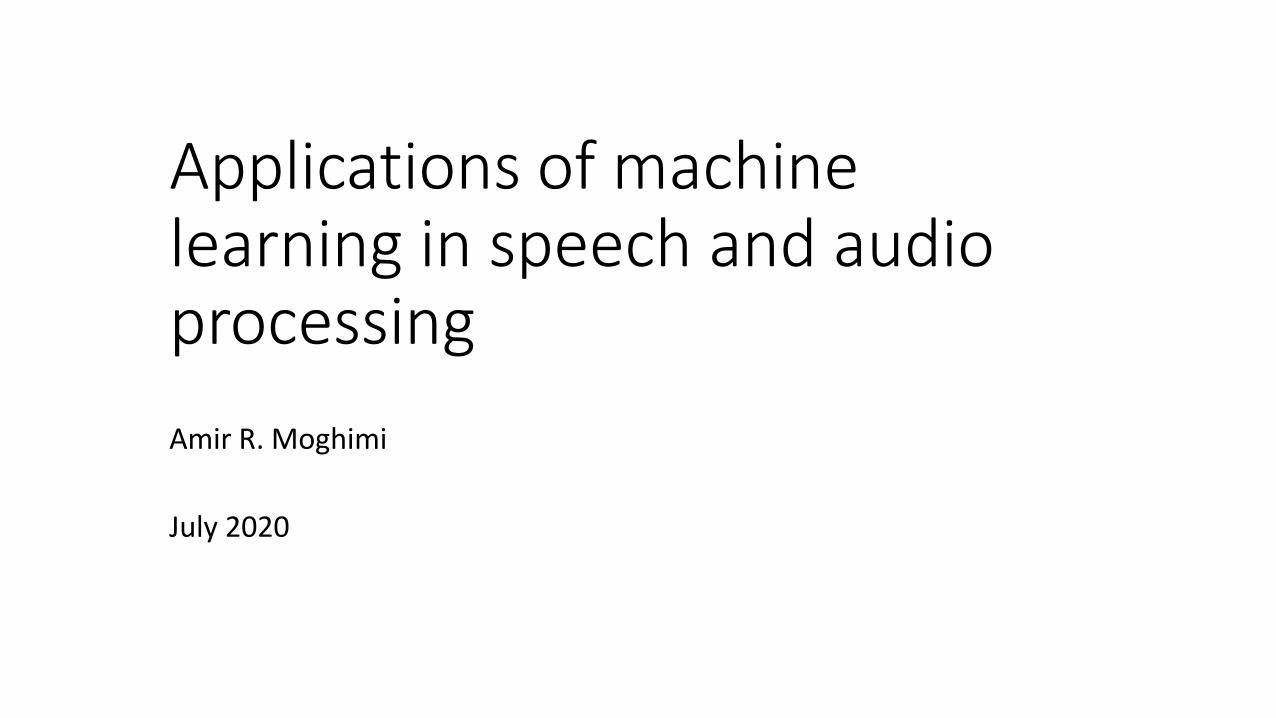
My background
Jan 2007 Jun 2014 May 2018
Nov 2019
Sep 2002
2
You are here
Topics for today
Automatic Speech Recognition (ASR)What someone is saying (audio → text)
Voice Activity Detection (VAD)Whether someone is speaking
Speech EnhancementMaking speech sound better
3
But first, a look at speech
4
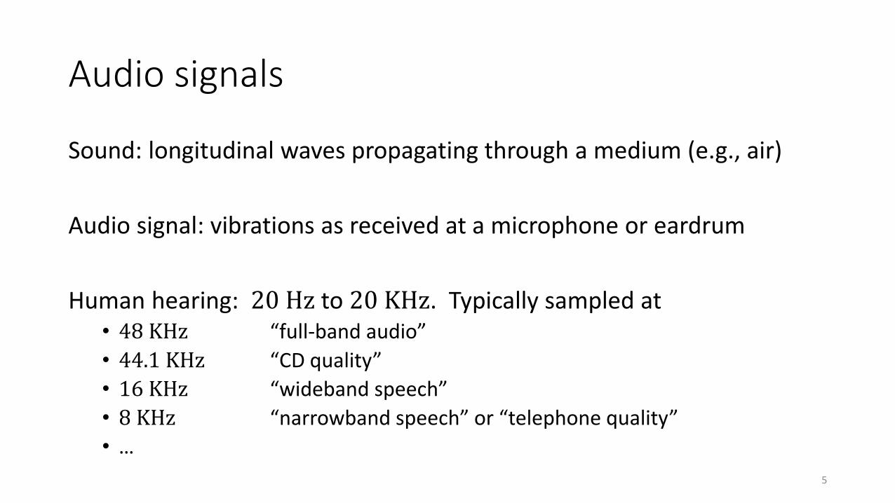
Audio signals
Sound: longitudinal waves propagating through a medium (e.g., air)
Audio signal: vibrations as received at a microphone or eardrum
Human hearing: 20 Hz to 20 KHz. Typically sampled at• 48 KHz “full-band audio”
• 44.1 KHz “CD quality”
• 16 KHz “wideband speech”
• 8 KHz “narrowband speech” or “telephone quality”
• …
5
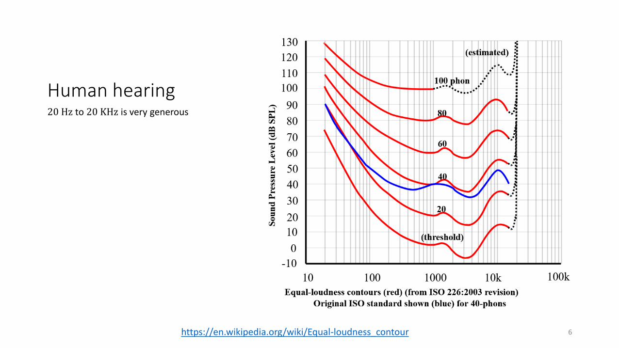
Human hearing20 Hz to 20 KHz is very generous
https://en.wikipedia.org/wiki/Equal-loudness_contour 6
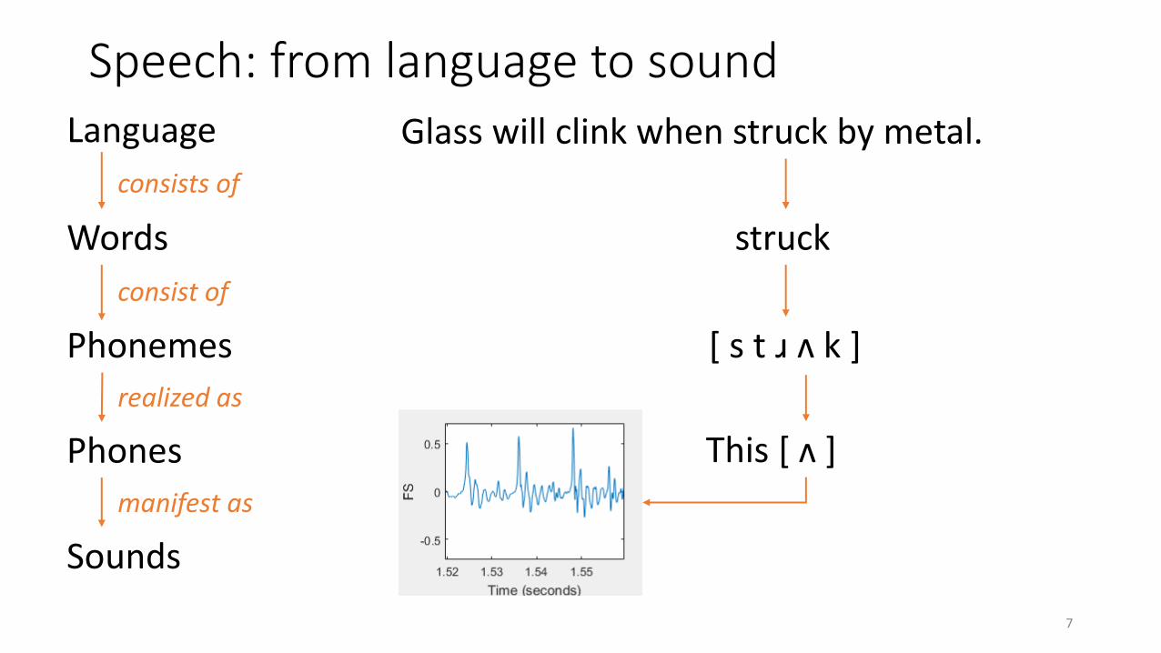
Speech: from language to sound
7
Language
Sounds
Words
Phonemes
Phones
consists of
consist of
realized as
manifest as
Glass will clink when struck by metal.
struck
[ s t ɹ ʌ k ]
This [ ʌ ]
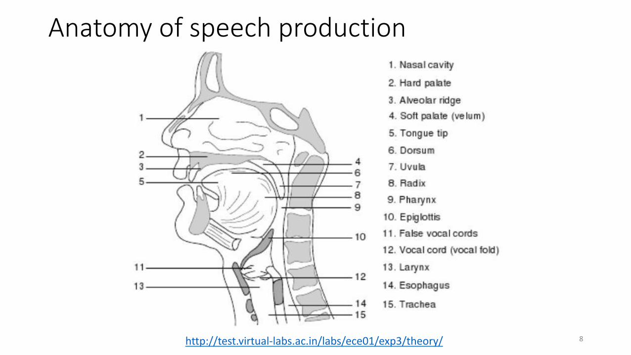
Anatomy of speech production
8http://test.virtual-labs.ac.in/labs/ece01/exp3/theory/
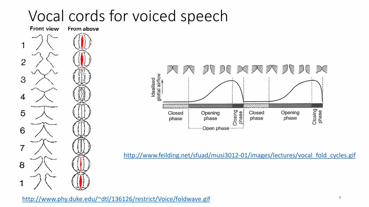
Vocal cords for voiced speech
9http://www.phy.duke.edu/~dtl/136126/restrict/Voice/foldwave.gif
http://www.feilding.net/sfuad/musi3012-01/images/lectures/vocal_fold_cycles.gif
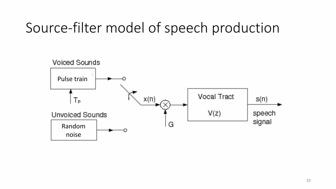
Source-filter model of speech production
10
Pulse train
Random noise
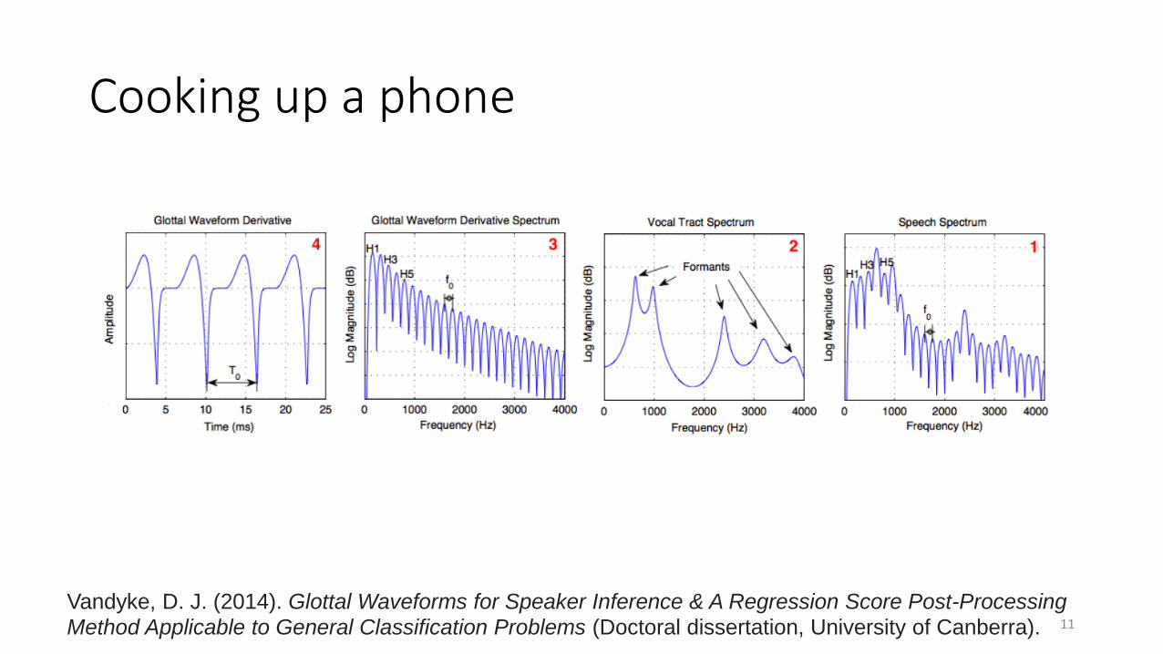
Cooking up a phone
11
Vandyke, D. J. (2014). Glottal Waveforms for Speaker Inference & A Regression Score Post-Processing
Method Applicable to General Classification Problems (Doctoral dissertation, University of Canberra).
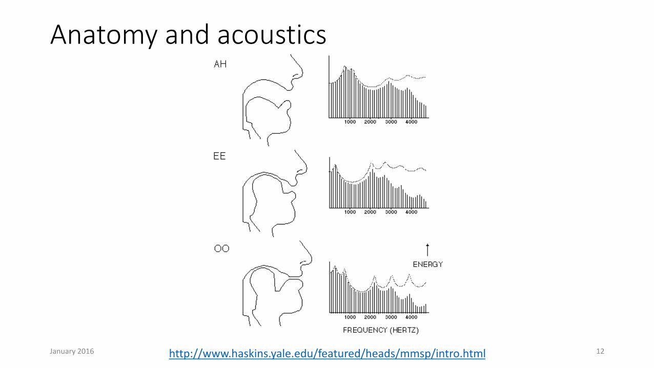
Anatomy and acoustics
January 2016 12http://www.haskins.yale.edu/featured/heads/mmsp/intro.html
/ɒ/ /i/ /u/ /m/
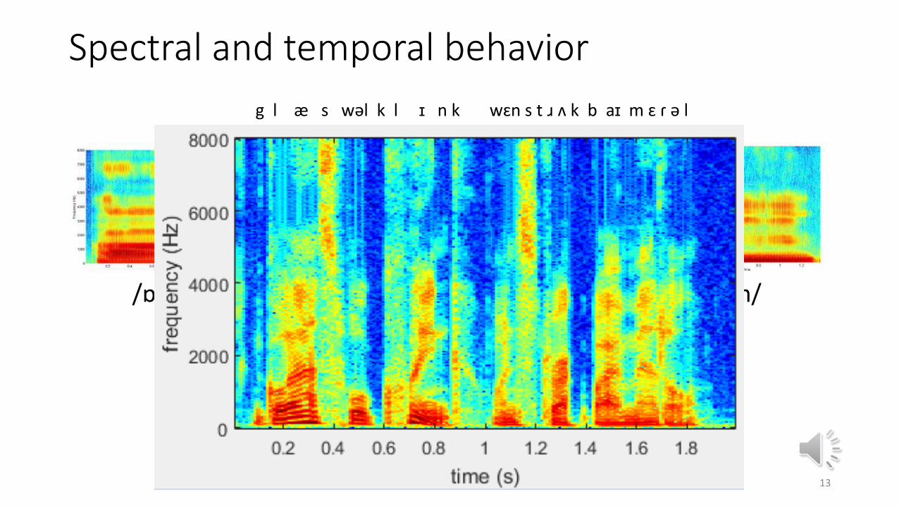
Spectral and temporal behavior
13
g l æ s wəl k l ɪ n k wɛn s t ɹ ʌ k b aɪ m ɛ ɾ ə l
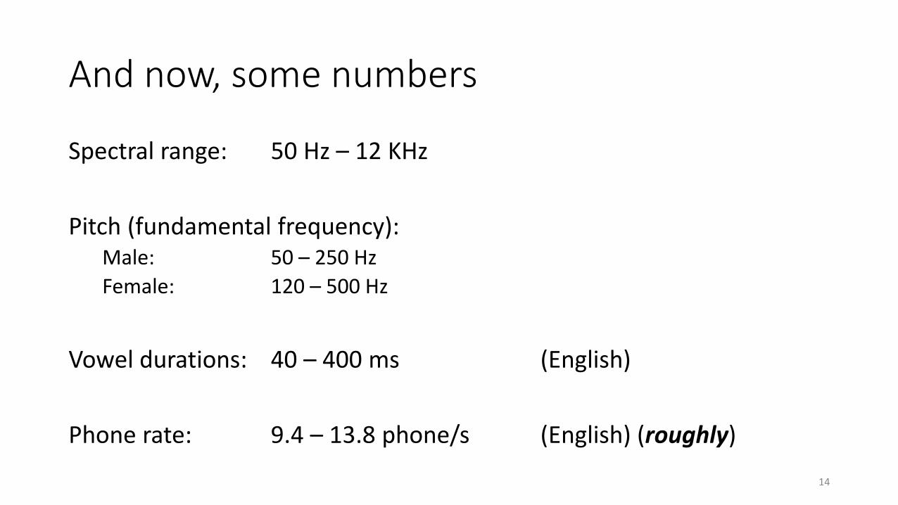
And now, some numbers
Spectral range: 50 Hz – 12 KHz
Pitch (fundamental frequency):Male: 50 – 250 Hz
Female: 120 – 500 Hz
Vowel durations: 40 – 400 ms (English)
Phone rate: 9.4 – 13.8 phone/s (English) (roughly)
14
Speech processing problems
15
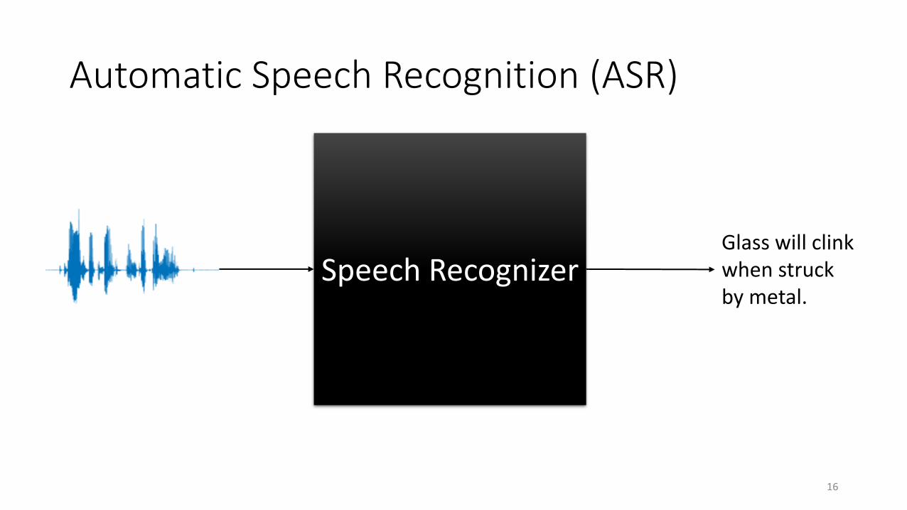
Automatic Speech Recognition (ASR)
16
Glass will clink when struck by metal.
Speech Recognizer
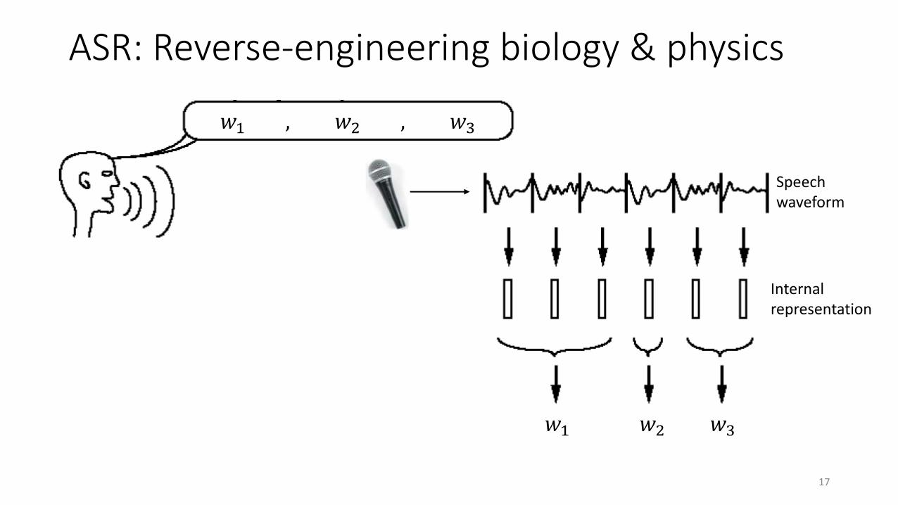
ASR: Reverse-engineering biology & physics
17
𝑤1 , 𝑤2 , 𝑤3
𝑤1 𝑤2 𝑤3
Speech waveform
Internal representation
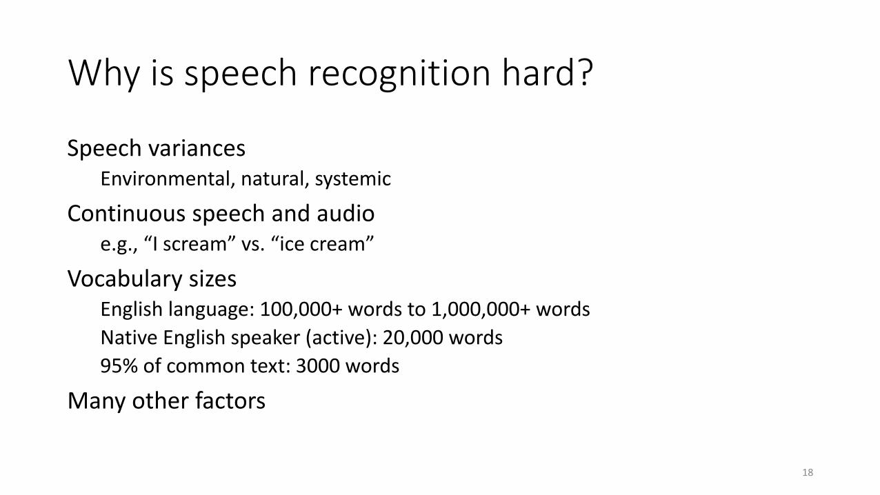
Why is speech recognition hard?
Speech variancesEnvironmental, natural, systemic
Continuous speech and audioe.g., “I scream” vs. “ice cream”
Vocabulary sizesEnglish language: 100,000+ words to 1,000,000+ words
Native English speaker (active): 20,000 words
95% of common text: 3000 words
Many other factors
18
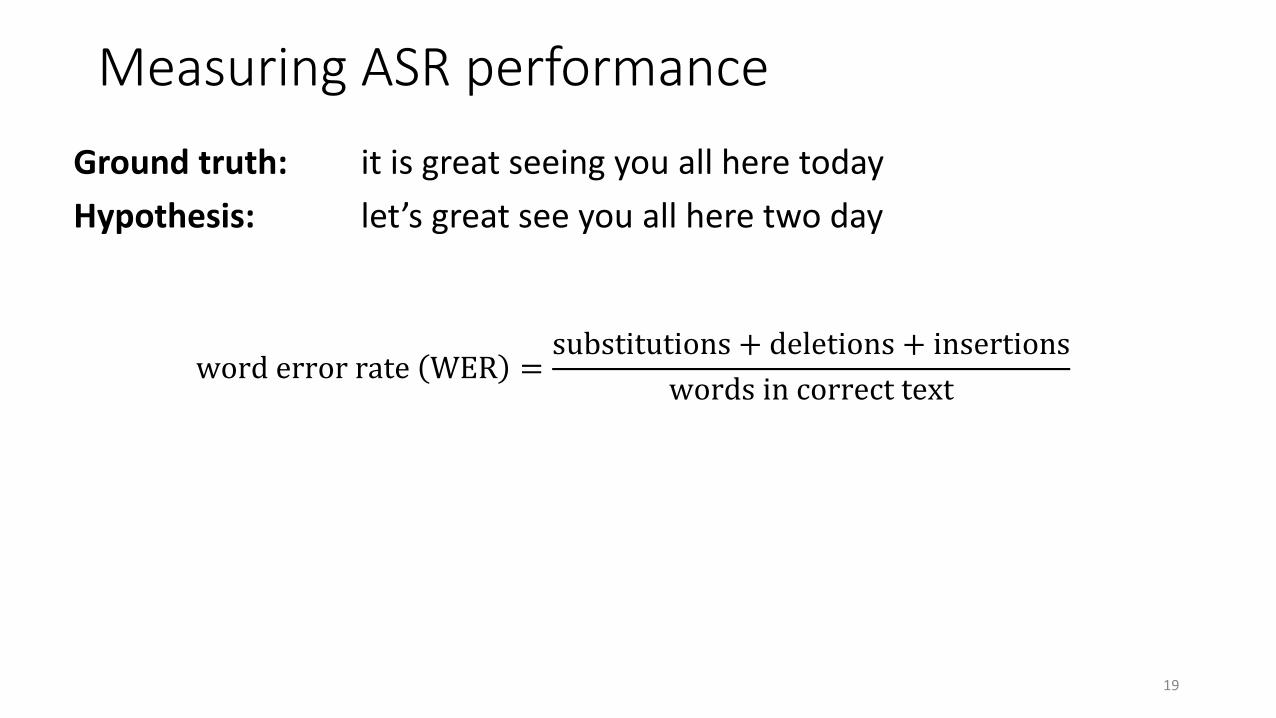
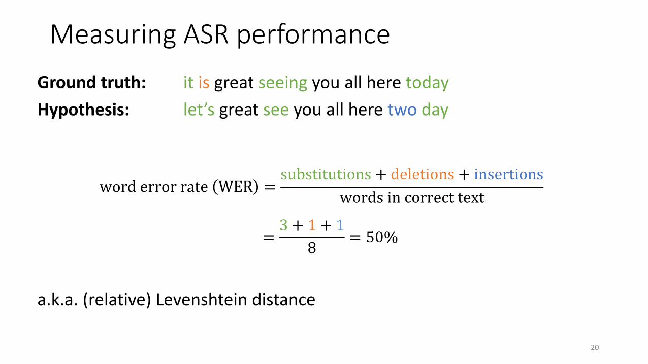
Measuring ASR performance
Ground truth: it is great seeing you all here today
Hypothesis: let’s great see you all here two day
19
word error rate WER =substitutions + deletions + insertions
words in correct text
Measuring ASR performance
Ground truth: it is great seeing you all here today
Hypothesis: let’s great see you all here two day
a.k.a. (relative) Levenshtein distance
20
word error rate WER =substitutions + deletions + insertions
words in correct text
=3 + 1 + 1
8= 50%
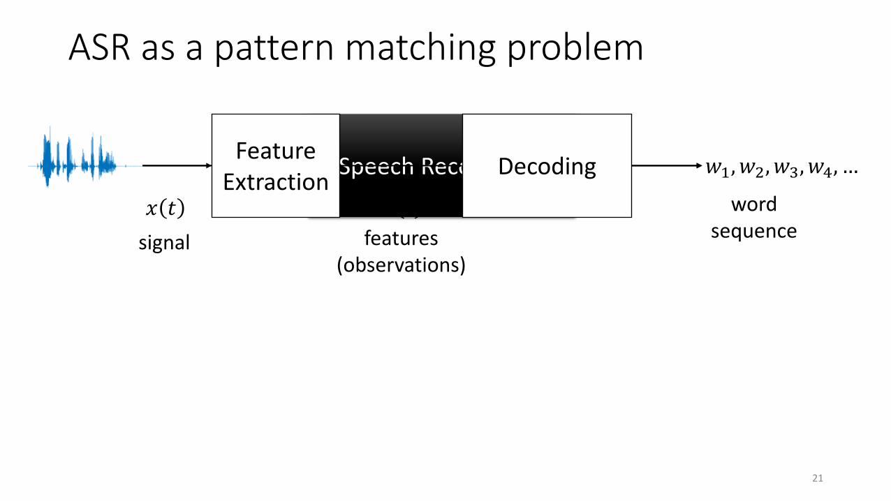
ASR as a pattern matching problem
21
Speech Recognition 𝑤1, 𝑤2, 𝑤3, 𝑤4, …Feature
ExtractionDecoding
𝑥 𝑡 𝐨 𝑡
signal features(observations)
word sequence
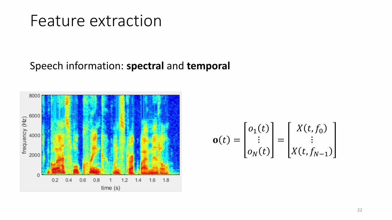
Feature extraction
Speech information: spectral and temporal
22
𝐨 𝑡 =𝑜1 𝑡⋮
𝑜𝑁 𝑡=
𝑋 𝑡, 𝑓0⋮
𝑋 𝑡, 𝑓𝑁−1

Commonly used speech features
Energy and pitch
Log power spectra
Linear Predictive Coding (LPC) coefficients
Mel-frequency Cepstral Coefficients (MFCC)
Perceptual Linear Prediction (PLP) coefficients
Power-normalized Cepstral Coefficients (PNCC)
…
23
Very early ASR
Template matchingCompare new recording to pre-recorded samples
Dynamic Time Warping (DTW)Allows for timing fluidity
24
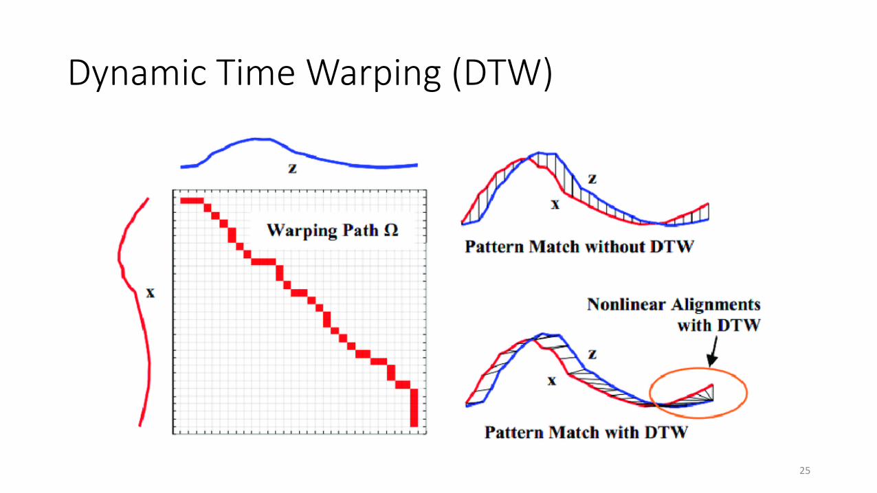
Dynamic Time Warping (DTW)
25
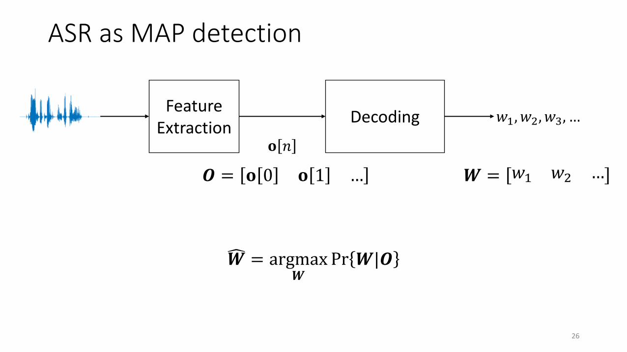
ASR as MAP detection
26
𝑤1, 𝑤2, 𝑤3, …Feature
ExtractionDecoding
𝐨 𝑛
𝑶 = 𝐨 0 𝐨 1 … 𝑾 = 𝑤1 𝑤2 …
𝑾 = argmax𝑾
Pr 𝑾|𝑶
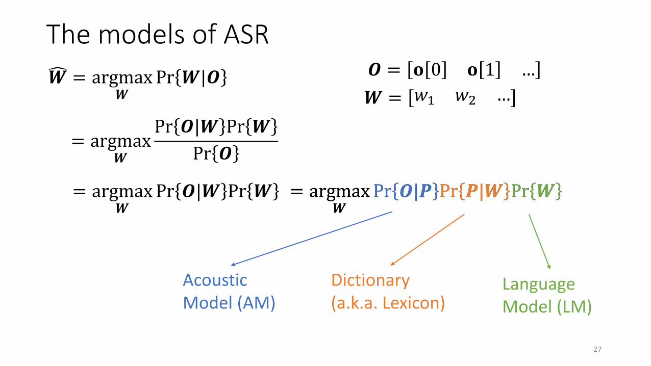
The models of ASR
27
= argmax𝑾
Pr 𝑶|𝑾 Pr 𝑾 = argmax𝑾
Pr 𝑶|𝑷 Pr 𝑷|𝑾 Pr 𝑾= argmax𝑾
Pr 𝑶|𝑷 Pr 𝑷|𝑾 Pr 𝑾
Acoustic Model (AM)
Dictionary (a.k.a. Lexicon)
Language Model (LM)
𝑾 = argmax𝑾
Pr 𝑾|𝑶
= argmax𝑾
Pr 𝑶|𝑾 Pr 𝑾
Pr 𝑶
𝑶 = 𝐨 0 𝐨 1 …
𝑾 = 𝑤1 𝑤2 …
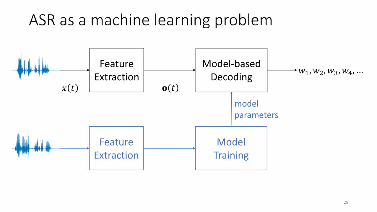
ASR as a machine learning problem
28
𝑤1, 𝑤2, 𝑤3, 𝑤4, …Feature
ExtractionModel-based
Decoding𝑥 𝑡 𝐨 𝑡
Feature Extraction
Model Training
model parameters
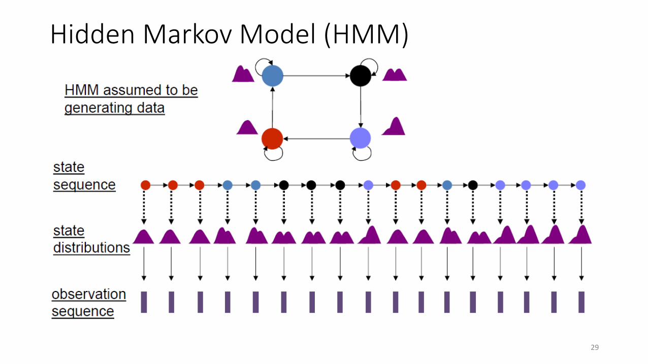
Hidden Markov Model (HMM)
29
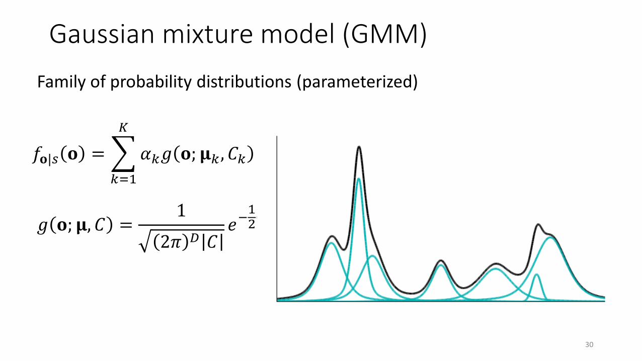
Gaussian mixture model (GMM)
Family of probability distributions (parameterized)
30
𝑔 𝐨; 𝛍, 𝐶 =1
2𝜋 𝐷 𝐶𝑒−
12 𝐨−𝛍 𝑇𝐶−1 𝐨−𝛍
𝑓𝐨|𝑠 𝐨 =
𝑘=1
𝐾
𝛼𝑘𝑔 𝐨; 𝛍𝑘 , 𝐶𝑘 ,
𝑘=1
𝐾
𝛼𝑘 = 1
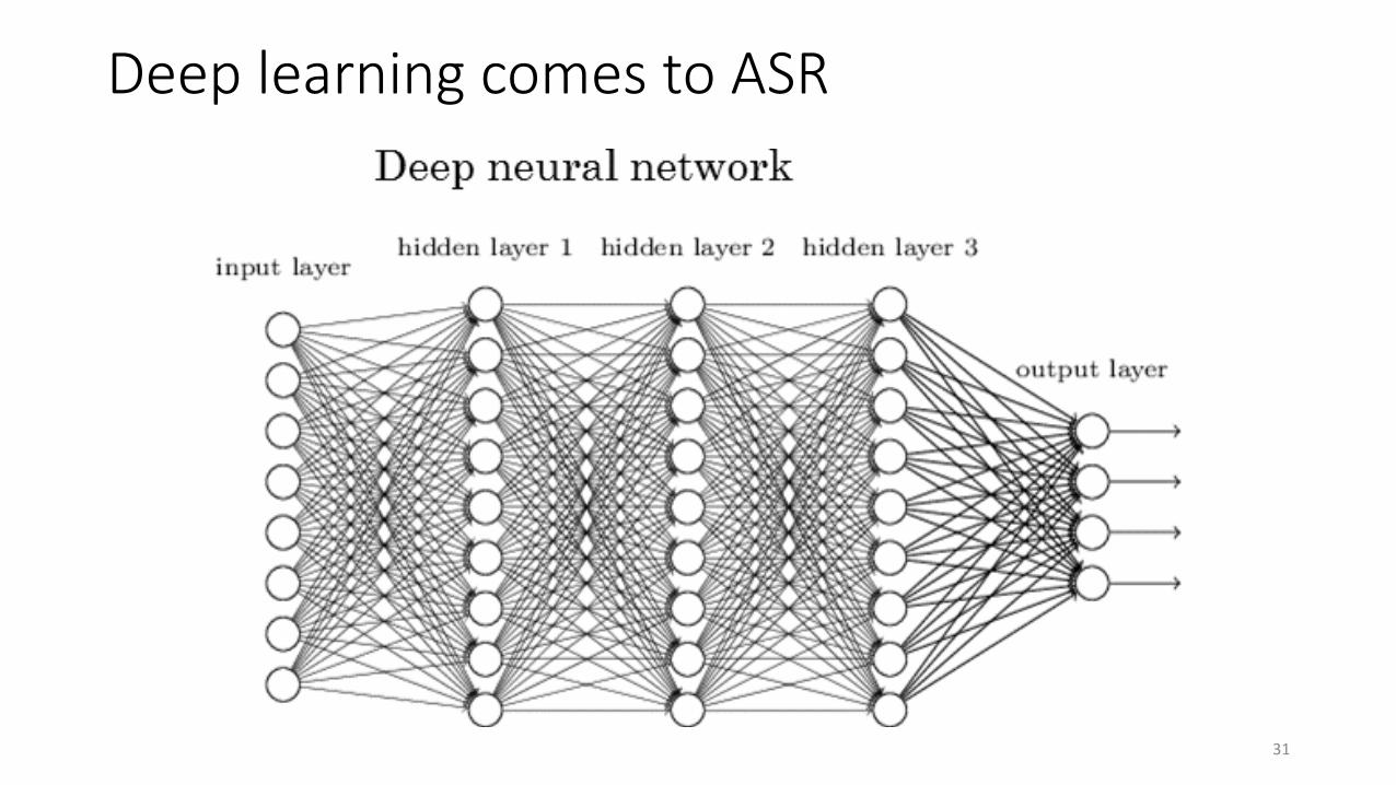
Deep learning comes to ASR
31
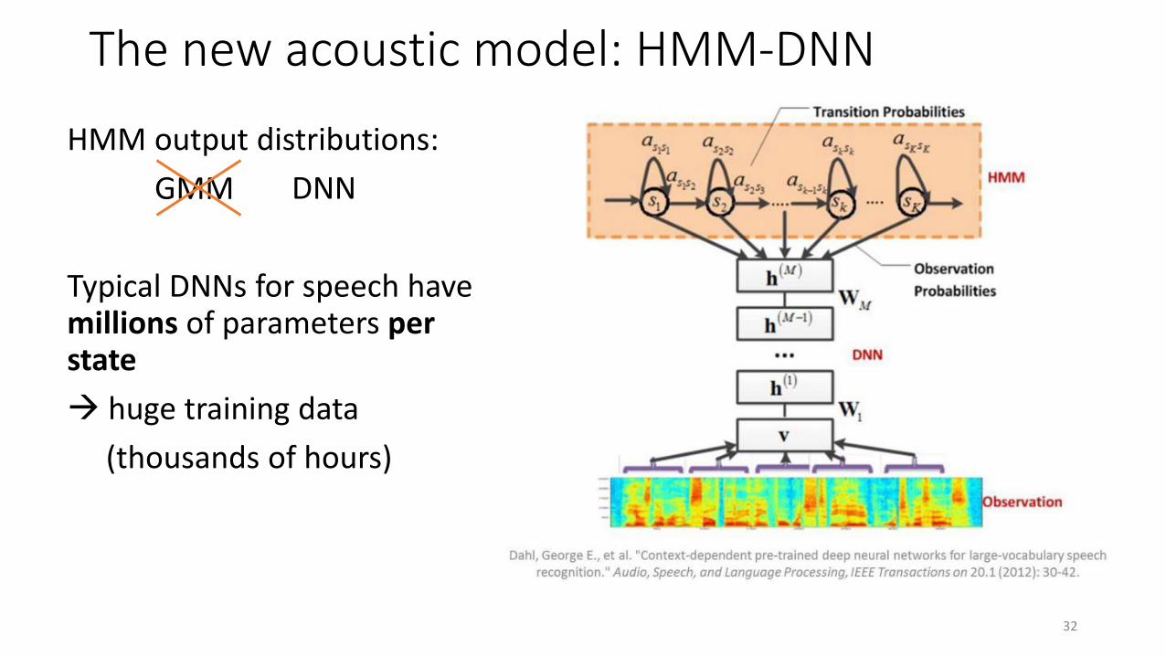
The new acoustic model: HMM-DNN
32
HMM output distributions:
GMM
Typical DNNs for speech have millions of parameters per state
→ huge training data
(thousands of hours)
DNN
Detour:Recurrent Neural Networks (RNNs)
33
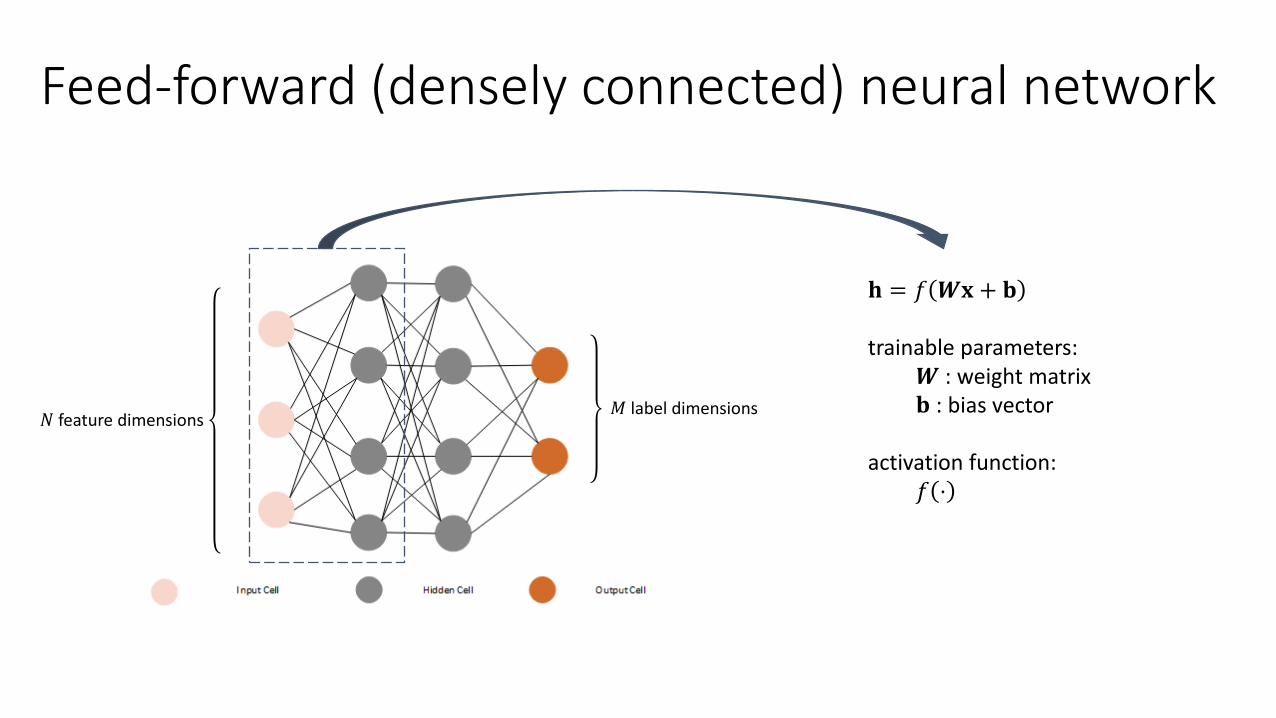
Feed-forward (densely connected) neural network
𝑁 feature dimensions 𝑀 label dimensions
𝐡 = 𝑓 𝑾𝐱 + 𝐛
trainable parameters:𝑾 : weight matrix𝐛 : bias vector
activation function:𝑓 ⋅
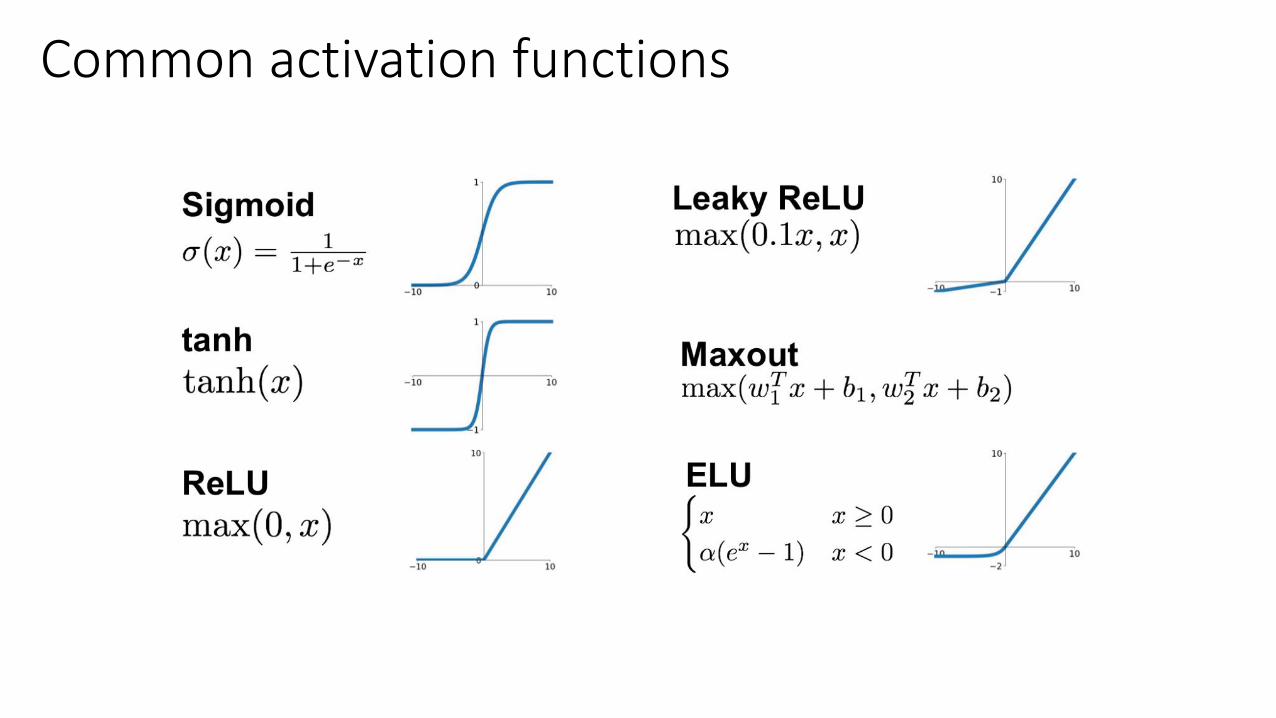
Common activation functions
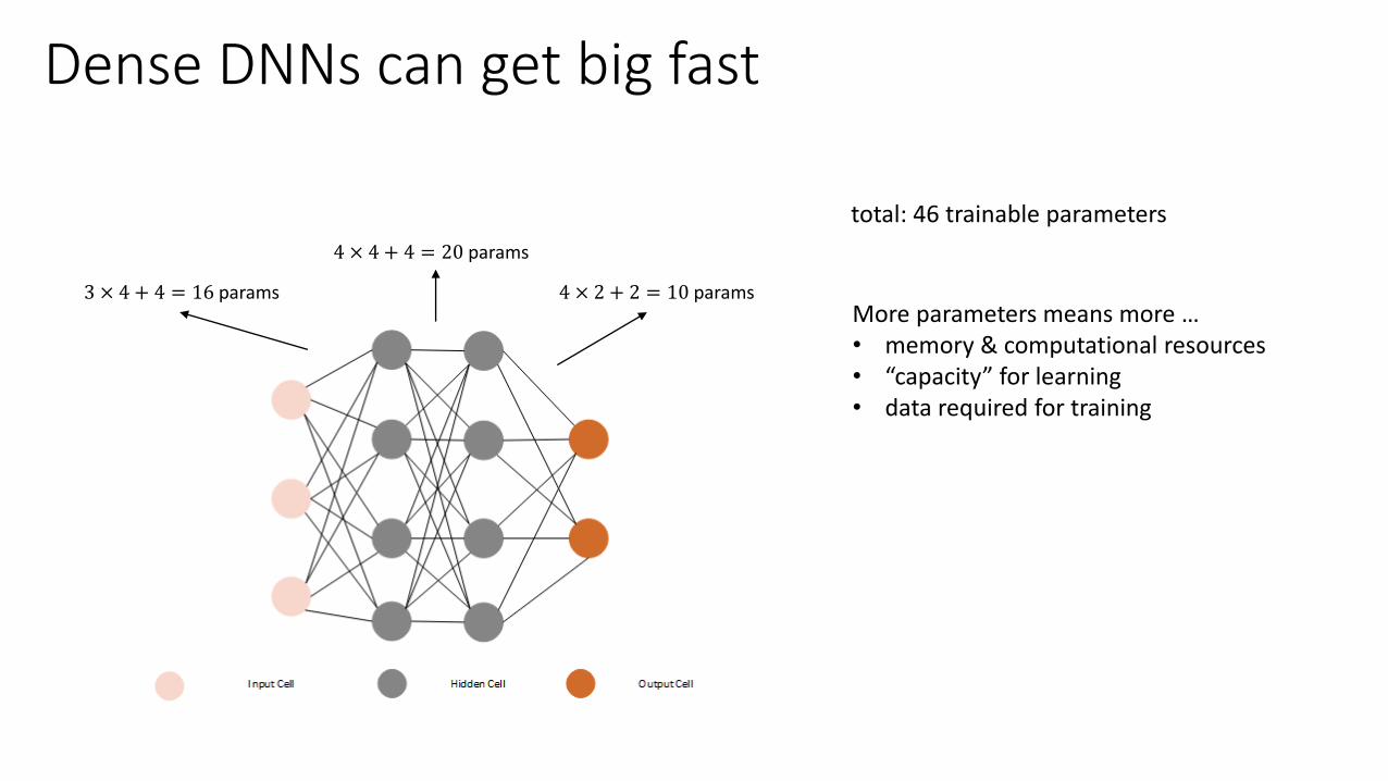
Dense DNNs can get big fast
3 × 4 + 4 = 16 params
4 × 4 + 4 = 20 params
4 × 2 + 2 = 10 params
total: 46 trainable parameters
More parameters means more …• memory & computational resources• “capacity” for learning• data required for training
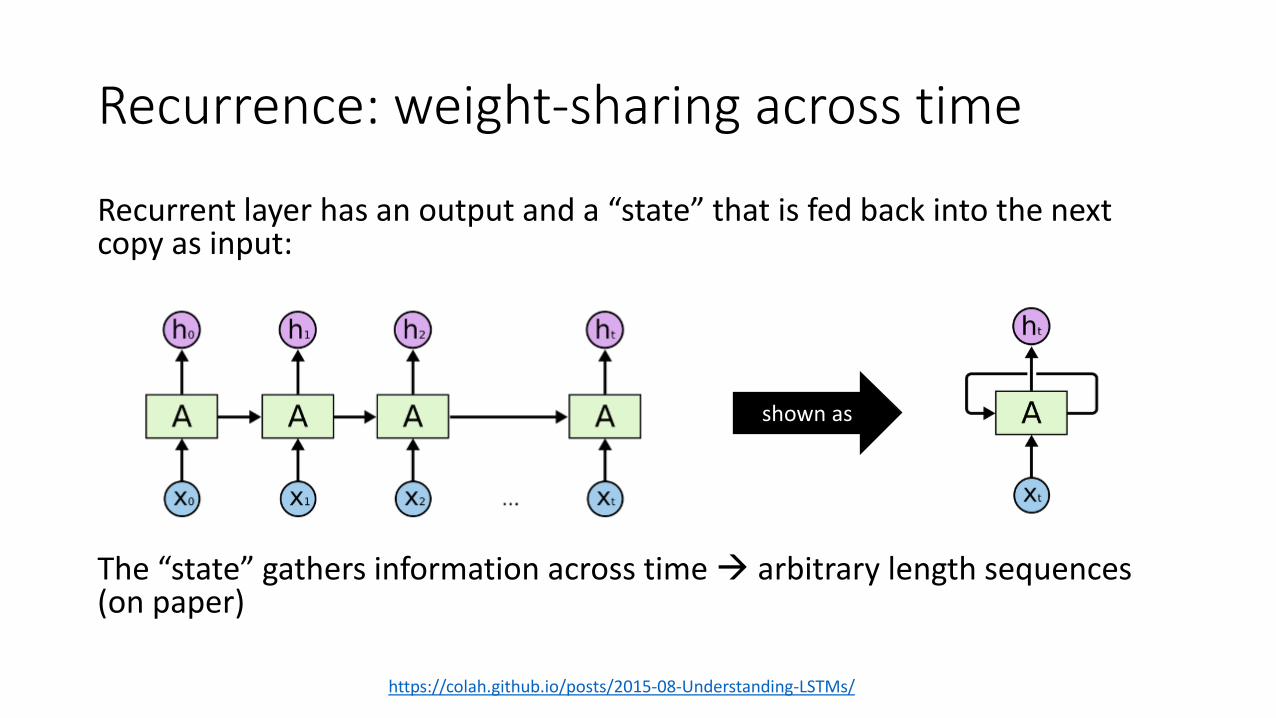
Recurrence: weight-sharing across time
Recurrent layer has an output and a “state” that is fed back into the next copy as input:
The “state” gathers information across time → arbitrary length sequences (on paper)
https://colah.github.io/posts/2015-08-Understanding-LSTMs/
shown as
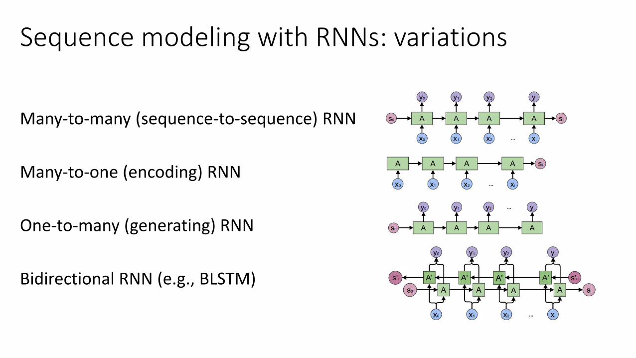
Many-to-many (sequence-to-sequence) RNN
Many-to-one (encoding) RNN
One-to-many (generating) RNN
Bidirectional RNN (e.g., BLSTM)
Sequence modeling with RNNs: variations

And now, back to our show
39
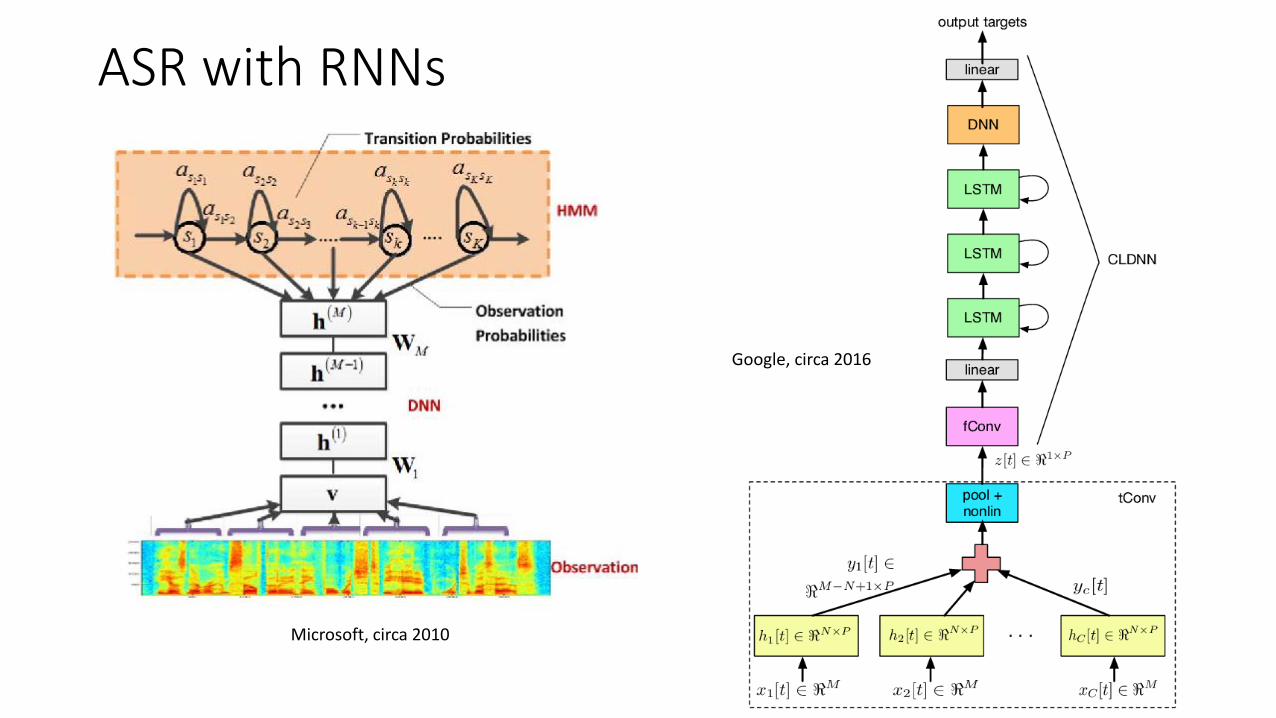
ASR with RNNs
40
Microsoft, circa 2010
Google, circa 2016
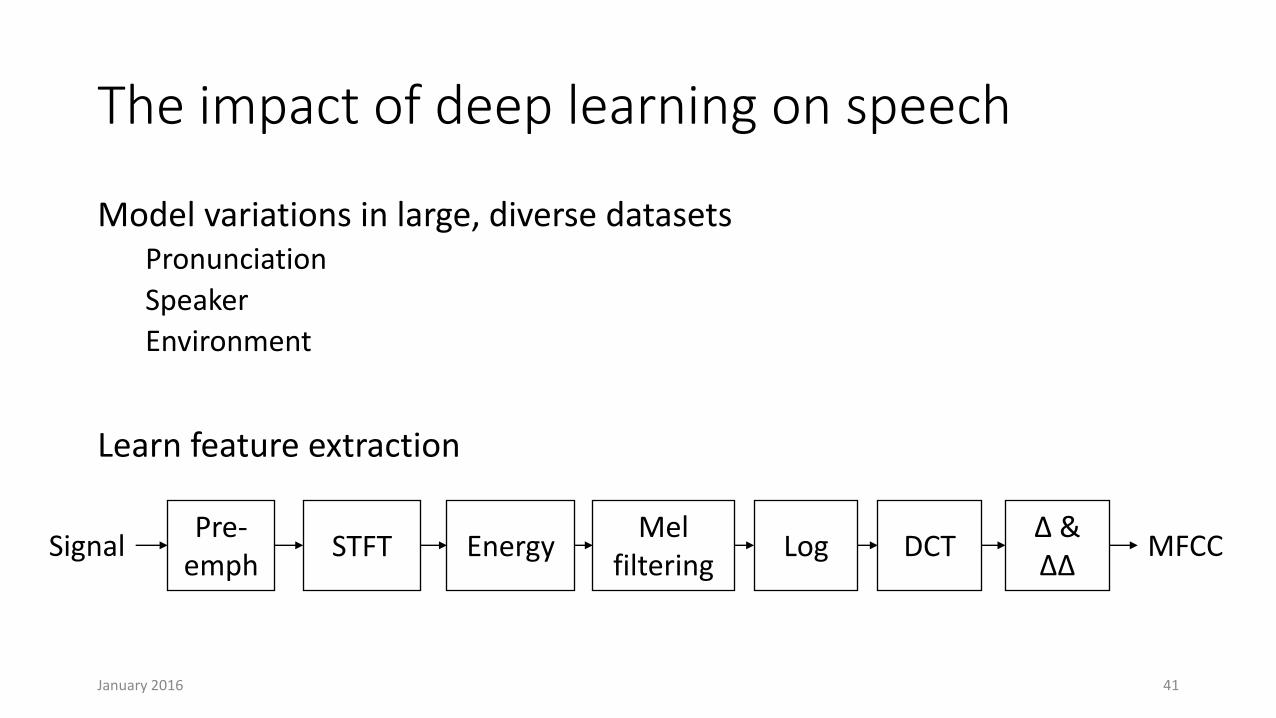
The impact of deep learning on speech
Model variations in large, diverse datasetsPronunciation
Speaker
Environment
Learn feature extraction
January 2016 41
Pre-emph
STFT EnergyMel
filteringLog DCT
Δ &ΔΔ
Signal MFCC
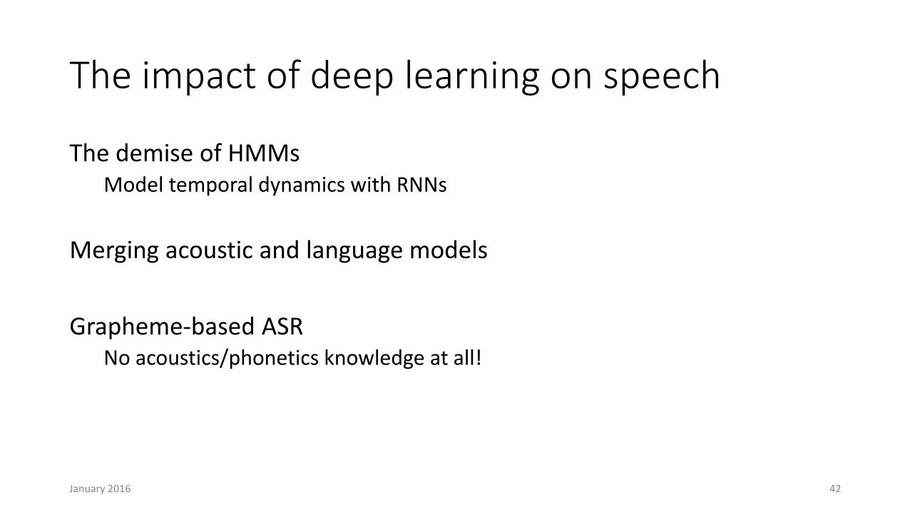
The impact of deep learning on speech
The demise of HMMsModel temporal dynamics with RNNs
Merging acoustic and language models
Grapheme-based ASRNo acoustics/phonetics knowledge at all!
January 2016 42
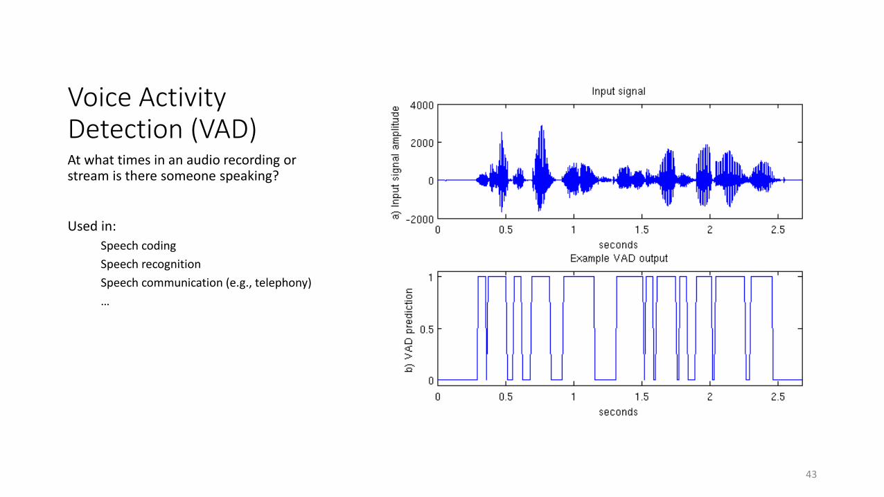
Voice Activity Detection (VAD)At what times in an audio recording or stream is there someone speaking?
Used in:
Speech coding
Speech recognition
Speech communication (e.g., telephony)
…
43
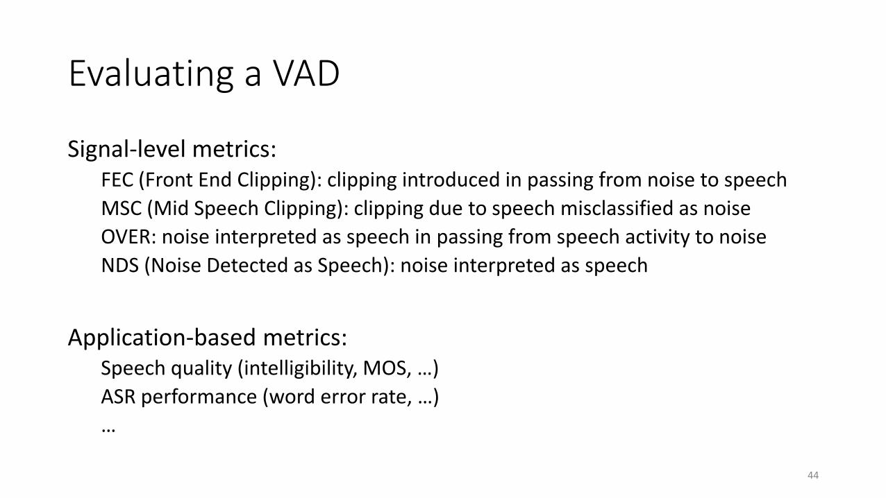
Evaluating a VAD
Signal-level metrics:FEC (Front End Clipping): clipping introduced in passing from noise to speech
MSC (Mid Speech Clipping): clipping due to speech misclassified as noise
OVER: noise interpreted as speech in passing from speech activity to noise
NDS (Noise Detected as Speech): noise interpreted as speech
Application-based metrics:Speech quality (intelligibility, MOS, …)
ASR performance (word error rate, …)
…
44
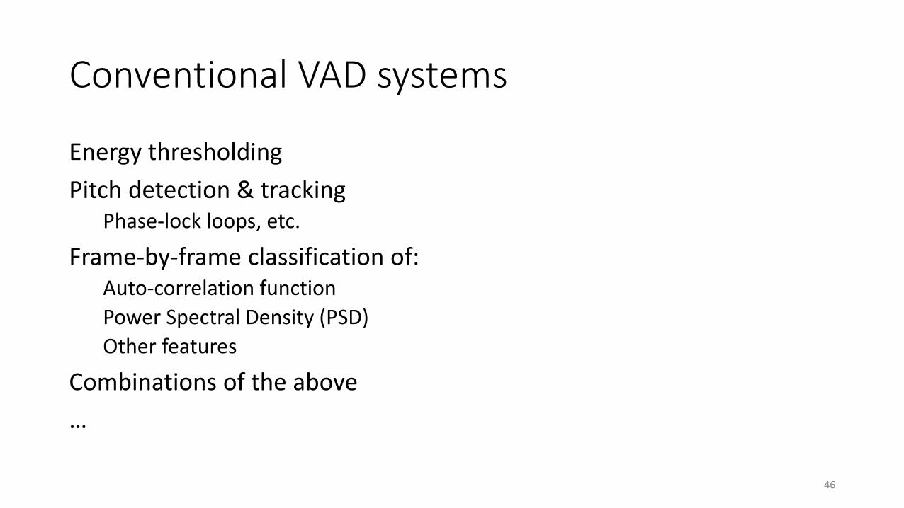
Conventional VAD systems
Energy thresholding
Pitch detection & trackingPhase-lock loops, etc.
Frame-by-frame classification of:Auto-correlation function
Power Spectral Density (PSD)
Other features
Combinations of the above
…
46
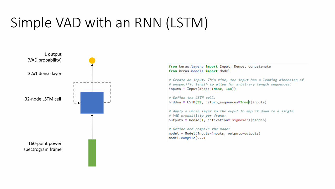
Simple VAD with an RNN (LSTM)
32x1 dense layer
32-node LSTM cell
1 output(VAD probability)
160-point power spectrogram frame
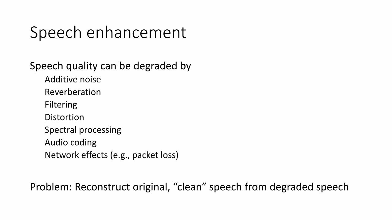
Speech enhancement
Speech quality can be degraded byAdditive noise
Reverberation
Filtering
Distortion
Spectral processing
Audio coding
Network effects (e.g., packet loss)
Problem: Reconstruct original, “clean” speech from degraded speech
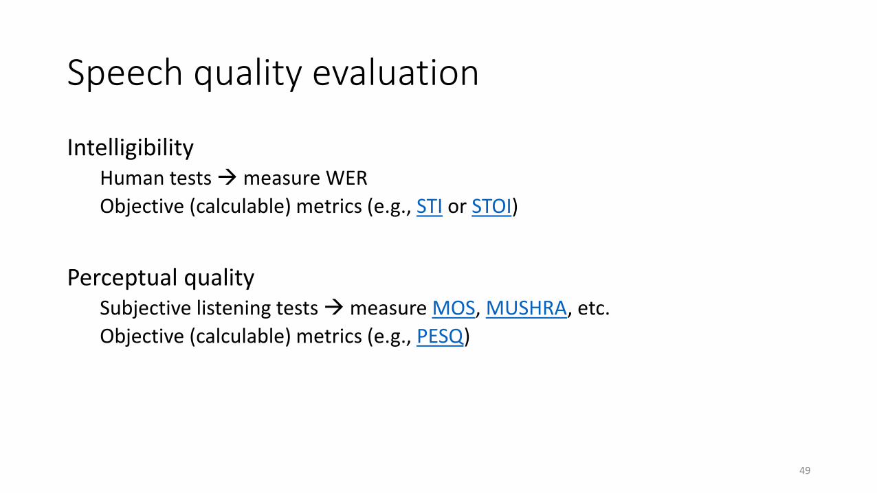
Speech quality evaluation
IntelligibilityHuman tests →measure WER
Objective (calculable) metrics (e.g., STI or STOI)
Perceptual qualitySubjective listening tests →measure MOS, MUSHRA, etc.
Objective (calculable) metrics (e.g., PESQ)
49
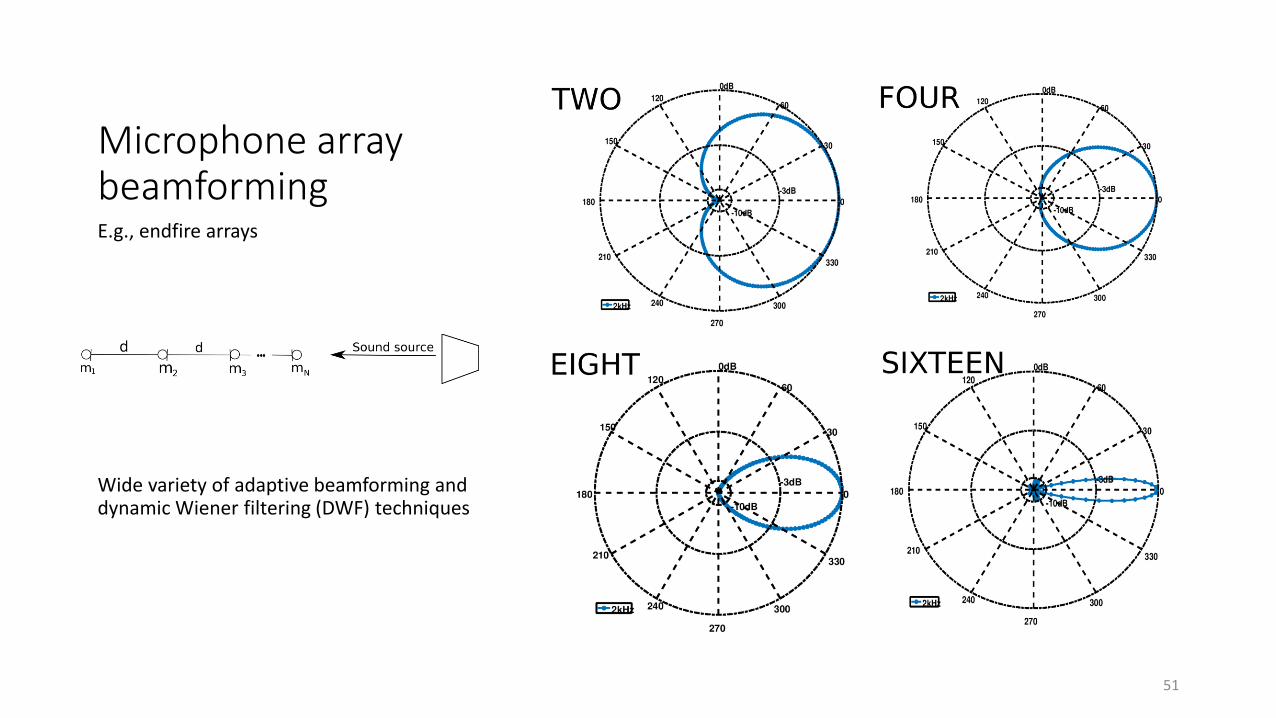
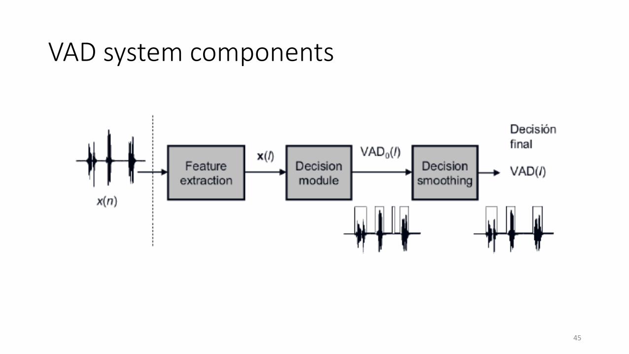
Microphone array beamformingE.g., endfire arrays
Wide variety of adaptive beamforming and dynamic Wiener filtering (DWF) techniques
51
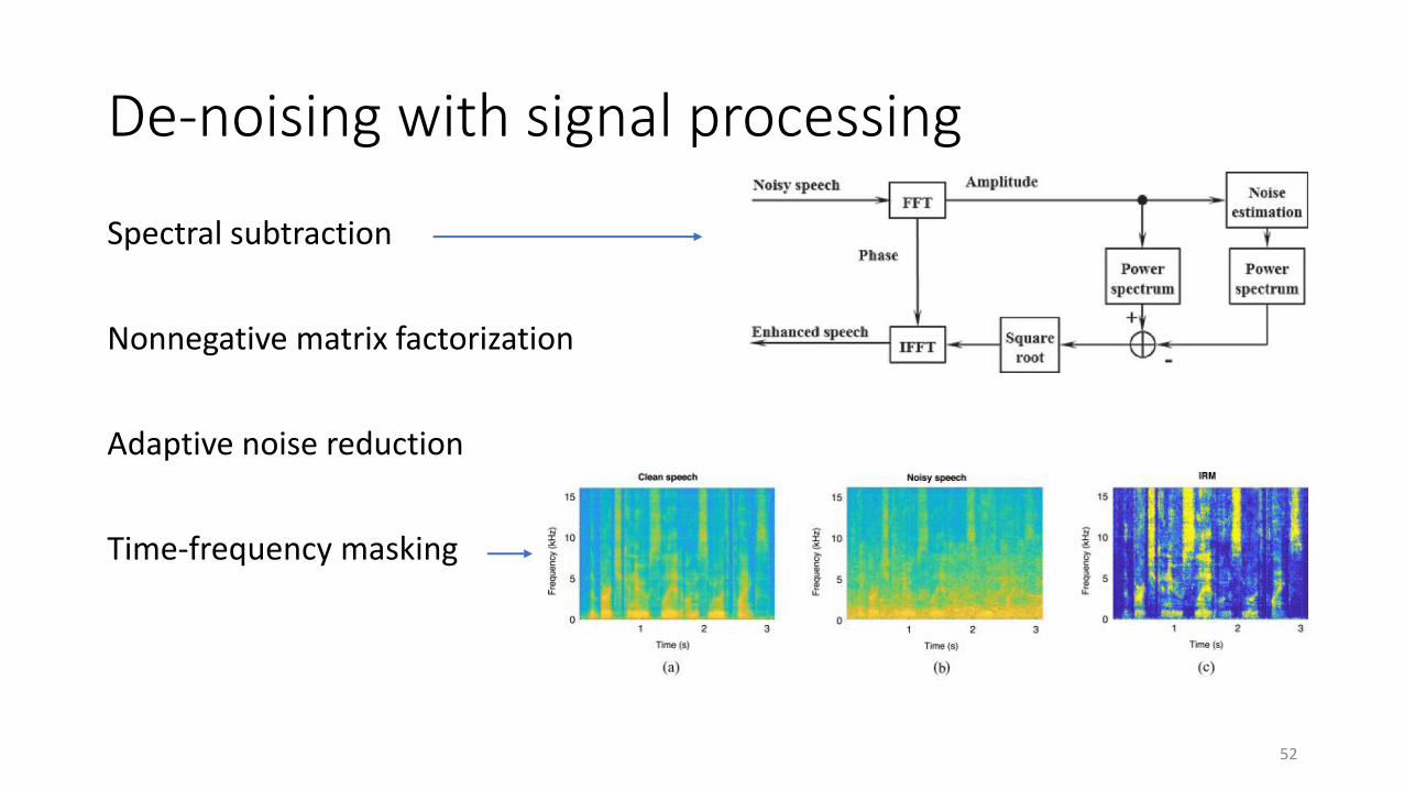
De-noising with signal processing
Spectral subtraction
Nonnegative matrix factorization
Adaptive noise reduction
Time-frequency masking
52
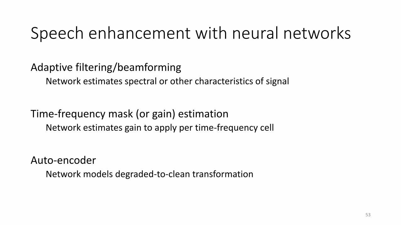
Speech enhancement with neural networks
Adaptive filtering/beamformingNetwork estimates spectral or other characteristics of signal
Time-frequency mask (or gain) estimationNetwork estimates gain to apply per time-frequency cell
Auto-encoderNetwork models degraded-to-clean transformation
53
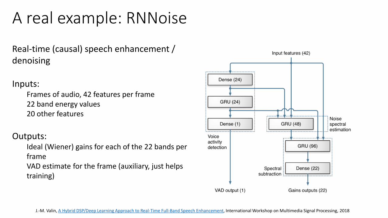
Real-time (causal) speech enhancement / denoising
Inputs: Frames of audio, 42 features per frame22 band energy values20 other features
Outputs:Ideal (Wiener) gains for each of the 22 bands per frameVAD estimate for the frame (auxiliary, just helps training)
A real example: RNNoise
J.-M. Valin, A Hybrid DSP/Deep Learning Approach to Real-Time Full-Band Speech Enhancement, International Workshop on Multimedia Signal Processing, 2018
Where we are now
Machine learning (especially deep learning) has completely overrun speech processing research
Promises of deep learning:Solves unsolvable problems
Finds unintuitive solutions
Removes the need for detailed expertise and handcrafting
Pitfalls of deep learning:Behavior difficult to explain/predict
Too easy to apply (and misapply)
Blind spots / false confidence / catastrophic failures

Thank you!
56