Embed Size (px)
Citation preview

Applications of Empirical Processes in Learning
Theory: Algorithmic Stability and Generalization
Bounds
by
Alexander Rakhlin
Submitted to the Department of Brain and Cognitive Sciencesin partial fulfillment of the requirements for the degree of
Doctor of Philosophy
at the
MASSACHUSETTS INSTITUTE OF TECHNOLOGY
June 2006
c© Massachusetts Institute of Technology 2006. All rights reserved.
Author . . . . . . . . . . . . . . . . . . . . . . . . . . . . . . . . . . . . . . . . . . . . . . . . . . . . . . . . . . . . . .Department of Brain and Cognitive Sciences
May 15, 2006
Certified by. . . . . . . . . . . . . . . . . . . . . . . . . . . . . . . . . . . . . . . . . . . . . . . . . . . . . . . . . .Tomaso Poggio
Eugene McDermott Professor of Brain SciencesThesis Supervisor
Accepted by . . . . . . . . . . . . . . . . . . . . . . . . . . . . . . . . . . . . . . . . . . . . . . . . . . . . . . . . .Matt Wilson
Head, Department Graduate Committee

2
Applications of Empirical Processes in Learning Theory:
Algorithmic Stability and Generalization Bounds
by
Alexander Rakhlin
Submitted to the Department of Brain and Cognitive Scienceson May 15, 2006, in partial fulfillment of the
requirements for the degree ofDoctor of Philosophy
Abstract
This thesis studies two key properties of learning algorithms: their generalizationability and their stability with respect to perturbations. To analyze these properties,we focus on concentration inequalities and tools from empirical process theory. Weobtain theoretical results and demonstrate their applications to machine learning.
First, we show how various notions of stability upper- and lower-bound the biasand variance of several estimators of the expected performance for general learningalgorithms. A weak stability condition is shown to be equivalent to consistency ofempirical risk minimization.
The second part of the thesis derives tight performance guarantees for greedyerror minimization methods – a family of computationally tractable algorithms. Inparticular, we derive risk bounds for a greedy mixture density estimation procedure.We prove that, unlike what is suggested in the literature, the number of terms in themixture is not a bias-variance trade-off for the performance.
The third part of this thesis provides a solution to an open problem regardingthe stability of Empirical Risk Minimization (ERM). This algorithm is of centralimportance in Learning Theory. By studying the suprema of the empirical process,we prove that ERM over Donsker classes of functions is stable in the L1 norm. Hence,as the number of samples grows, it becomes less and less likely that a perturbation ofo(√
n) samples will result in a very different empirical minimizer. Asymptotic ratesof this stability are proved under metric entropy assumptions on the function class.Through the use of a ratio limit inequality, we also prove stability of expected errorsof empirical minimizers. Next, we investigate applications of the stability result. Inparticular, we focus on procedures that optimize an objective function, such as k-means and other clustering methods. We demonstrate that stability of clustering,just like stability of ERM, is closely related to the geometry of the class and theunderlying measure. Furthermore, our result on stability of ERM delineates a phasetransition between stability and instability of clustering methods.
In the last chapter, we prove a generalization of the bounded-difference concentra-tion inequality for almost-everywhere smooth functions. This result can be utilized to
3
analyze algorithms which are almost always stable. Next, we prove a phase transitionin the concentration of almost-everywhere smooth functions. Finally, a tight concen-tration of empirical errors of empirical minimizers is shown under an assumption onthe underlying space.
Thesis Supervisor: Tomaso PoggioTitle: Eugene McDermott Professor of Brain Sciences
4

TO MY PARENTS
5

Acknowledgments
I would like to start by thanking Tomaso Poggio for advising me throughout my years
at MIT. Unlike applied projects, where progress is observed continuously, theoretical
research requires a certain time until the known results are understood and the new
results start to appear. I thank Tommy for believing in my abilities and allowing me
to work on interesting open-ended theoretical problems. Additionally, I am grateful
to Tommy for introducing me to the multi-disciplinary approach to learning.
Many thanks go to Dmitry Panchenko. It is after his class that I became very
interested in Statistical Learning Theory. Numerous discussions with Dmitry shaped
the direction of my research. I very much value his encouragement and support all
these years.
I thank Andrea Caponnetto for being a great teacher, colleague, and a friend.
Thanks for the discussions about everything – from philosophy to Hilbert spaces.
I owe many thanks to Sayan Mukherjee, who supported me since my arrival at
MIT. He always found problems for me to work on and a pint of beer when I felt
down.
Very special thanks to Shahar Mendelson, who invited me to Australia. Shahar
taught me the geometric style of thinking, as well as a great deal of math. He also
taught me to publish only valuable results instead of seeking to lengthen my CV.
I express my deepest gratitude to Petra Philips.
Thanks to Gadi for the wonderful coffee and interesting conversations; thanks to
Mary Pat for her help on the administrative front; thanks to all the past and present
CBCL members, especially Gene.
I thank the Student Art Association for providing the opportunity to make pottery
and release stress; thanks to the CSAIL hockey team for keeping me in shape.
I owe everything to my friends. Without you, my life in Boston would have been
dull. Lots of thanks to Dima, Essie, Max, Sashka, Yanka & Dimka, Marina, Shok,
and many others. Special thanks to Dima, Lena, and Sasha for spending many hours
fixing my grammar. Thanks to Lena for her support.
6

Finally, I would like to express my deepest appreciation to my parents for every-
thing they have done for me.
7

8

Contents
1 Theory of Learning: Introduction 17
1.1 The Learning Problem . . . . . . . . . . . . . . . . . . . . . . . . . . 18
1.2 Generalization Bounds . . . . . . . . . . . . . . . . . . . . . . . . . . 20
1.3 Algorithmic Stability . . . . . . . . . . . . . . . . . . . . . . . . . . . 21
1.4 Overview . . . . . . . . . . . . . . . . . . . . . . . . . . . . . . . . . . 23
1.5 Contributions . . . . . . . . . . . . . . . . . . . . . . . . . . . . . . . 24
2 Preliminaries 27
2.1 Notation and Definitions . . . . . . . . . . . . . . . . . . . . . . . . . 27
2.2 Estimates of the Performance . . . . . . . . . . . . . . . . . . . . . . 30
2.2.1 Uniform Convergence of Means to Expectations . . . . . . . . 32
2.2.2 Algorithmic Stability . . . . . . . . . . . . . . . . . . . . . . . 33
2.3 Some Algorithms . . . . . . . . . . . . . . . . . . . . . . . . . . . . . 34
2.3.1 Empirical Risk Minimization . . . . . . . . . . . . . . . . . . . 34
2.3.2 Regularization Algorithms . . . . . . . . . . . . . . . . . . . . 34
2.3.3 Boosting Algorithms . . . . . . . . . . . . . . . . . . . . . . . 36
2.4 Concentration Inequalities . . . . . . . . . . . . . . . . . . . . . . . . 37
2.5 Empirical Process Theory . . . . . . . . . . . . . . . . . . . . . . . . 42
2.5.1 Covering and Packing Numbers . . . . . . . . . . . . . . . . . 42
2.5.2 Donsker and Glivenko-Cantelli Classes . . . . . . . . . . . . . 43
2.5.3 Symmetrization and Concentration . . . . . . . . . . . . . . . 45
9

3 Generalization Bounds via Stability 47
3.1 Introduction . . . . . . . . . . . . . . . . . . . . . . . . . . . . . . . . 47
3.2 Historical Remarks and Motivation . . . . . . . . . . . . . . . . . . . 49
3.3 Bounding Bias and Variance . . . . . . . . . . . . . . . . . . . . . . . 51
3.3.1 Decomposing the Bias . . . . . . . . . . . . . . . . . . . . . . 51
3.3.2 Bounding the Variance . . . . . . . . . . . . . . . . . . . . . . 53
3.4 Bounding the 2nd Moment . . . . . . . . . . . . . . . . . . . . . . . . 55
3.4.1 Leave-one-out (Deleted) Estimate . . . . . . . . . . . . . . . . 56
3.4.2 Empirical Error (Resubstitution) Estimate: Replacement Case 58
3.4.3 Empirical Error (Resubstitution) Estimate . . . . . . . . . . . 60
3.4.4 Resubstitution Estimate for the Empirical Risk Minimization
Algorithm . . . . . . . . . . . . . . . . . . . . . . . . . . . . . 62
3.5 Lower Bounds . . . . . . . . . . . . . . . . . . . . . . . . . . . . . . . 64
3.6 Rates of Convergence . . . . . . . . . . . . . . . . . . . . . . . . . . . 65
3.6.1 Uniform Stability . . . . . . . . . . . . . . . . . . . . . . . . . 65
3.6.2 Extending McDiarmid’s Inequality . . . . . . . . . . . . . . . 67
3.7 Summary and Open Problems . . . . . . . . . . . . . . . . . . . . . . 69
4 Performance of Greedy Error Minimization Procedures 71
4.1 General Results . . . . . . . . . . . . . . . . . . . . . . . . . . . . . . 71
4.2 Density Estimation . . . . . . . . . . . . . . . . . . . . . . . . . . . . 76
4.2.1 Main Results . . . . . . . . . . . . . . . . . . . . . . . . . . . 78
4.2.2 Discussion of the Results . . . . . . . . . . . . . . . . . . . . . 80
4.2.3 Proofs . . . . . . . . . . . . . . . . . . . . . . . . . . . . . . . 82
4.3 Classification . . . . . . . . . . . . . . . . . . . . . . . . . . . . . . . 88
5 Stability of Empirical Risk Minimization over Donsker Classes 91
5.1 Introduction . . . . . . . . . . . . . . . . . . . . . . . . . . . . . . . . 91
5.2 Notation . . . . . . . . . . . . . . . . . . . . . . . . . . . . . . . . . . 94
5.3 Main Result . . . . . . . . . . . . . . . . . . . . . . . . . . . . . . . . 95
5.4 Stability of almost-ERM . . . . . . . . . . . . . . . . . . . . . . . . . 98
10

5.5 Rates of Decay of diamMξ(n)S . . . . . . . . . . . . . . . . . . . . . . 101
5.6 Expected Error Stability of almost-ERM . . . . . . . . . . . . . . . . 104
5.7 Applications . . . . . . . . . . . . . . . . . . . . . . . . . . . . . . . . 104
5.7.1 Finding the Least (or Most) Dense Region . . . . . . . . . . . 105
5.7.2 Clustering . . . . . . . . . . . . . . . . . . . . . . . . . . . . . 106
5.8 Conclusions . . . . . . . . . . . . . . . . . . . . . . . . . . . . . . . . 112
6 Concentration and Stability 115
6.1 Concentration of Almost-Everywhere Smooth Functions . . . . . . . . 115
6.2 The Bad Set . . . . . . . . . . . . . . . . . . . . . . . . . . . . . . . . 120
6.2.1 Main Result . . . . . . . . . . . . . . . . . . . . . . . . . . . . 121
6.2.2 Symmetric Functions . . . . . . . . . . . . . . . . . . . . . . . 126
6.3 Concentration of Measure: Application of Inequality of Bobkov-Ledoux 128
A Technical Proofs 131
11

12

List of Figures
2-1 Fitting the data. . . . . . . . . . . . . . . . . . . . . . . . . . . . . . 32
2-2 Multiple minima of the empirical risk: two dissimilar functions fit the
data. . . . . . . . . . . . . . . . . . . . . . . . . . . . . . . . . . . . . 35
2-3 Unique minimum of the regularized fit to the data. . . . . . . . . . . 36
2-4 Probability surface . . . . . . . . . . . . . . . . . . . . . . . . . . . . 41
4-1 Step-up and step-down functions on the [0, 1] interval . . . . . . . . . 75
4-2 Convex loss ` upper-bounds the indicator loss. . . . . . . . . . . . . . 89
5-1 Realizable setting. . . . . . . . . . . . . . . . . . . . . . . . . . . . . . 96
5-2 Single minimum of expected error. . . . . . . . . . . . . . . . . . . . . 96
5-3 Finite number of minimizers of expected error. . . . . . . . . . . . . . 96
5-4 Infinitely many minimizers of expected error. . . . . . . . . . . . . . . 96
5-5 The most dense region of a fixed size. . . . . . . . . . . . . . . . . . . 105
5-6 The clustering objective is to place the centers Zk to minimize the sum
of squared distances from points to their closest centers. . . . . . . . 108
5-7 To prove Lemma 5.7.1 it is enough to show that the shaded area is
upperbounded by the L1 distance between the functions ha1,...,aKand
hb1,...,bKand lower-bounded by a power of d. We deduce that d cannot
be large. . . . . . . . . . . . . . . . . . . . . . . . . . . . . . . . . . . 111
6-1 Function f defined at the vertices as −1 or 1 such that Ef = 0. . . . 122
13

6-2 n-dimensional cube with a −1, 1-valued function defined on the ver-
tices. The dashed line is the boundary separating the set of −1’s from
the set of 1’s. The points at the boundary are the “bad set”. . . . . . 123
6-3 The boundary is smallest when the cube is cut in the middle. The
extremal set is the set of points at most n/2-Hamming distance away
from the origin. . . . . . . . . . . . . . . . . . . . . . . . . . . . . . . 123
14

List of Tables
2.1 Table of notation . . . . . . . . . . . . . . . . . . . . . . . . . . . . . 30
15

16

Chapter 1
Theory of Learning: Introduction
Intelligence is a very general mental capability that, among other things, involves the
ability to reason, plan, solve problems, think abstractly, comprehend complex ideas,
learn quickly and learn from experience. It is not merely book learning, a narrow
academic skill, or test-taking smarts. Rather, it reflects a broader and deeper capability
for comprehending our surroundings –“catching on,” “making sense” of things, or
“figuring out” what to do. [30]
The quest for building intelligent computer systems started in the 1950’s, when
the term “artificial intelligence” (AI) was first coined by John McCarthy. Since
then, major achievements have been made, ranging from medical diagnosis systems to
the Deep Blue chess playing program that beat the world champion Gary Kasparov
in 1997. However, when measured against the definition above, the advances in
Artificial Intelligence are still distant from their goal. It can be argued that, although
the current systems can reason, plan, and solve problems in particular constrained
domains, it is the “learning” part that stands out as an obstacle to overcome.
Machine learning has been an extremely active area of research in the past fifteen
years. Since the pioneering work of Vapnik and Chervonenkis, theoretical foundations
of learning have been laid out and numerous successful algorithms developed. This
thesis aims to add to our understanding of the theory behind learning processes.
The problem of learning is often formalized within a probabilistic setting. Once
such a mathematical framework is set, the following questions can be attacked:
17

How many examples are needed to accurately learn a concept? Will a given system
be likely to give a correct answer on an unseen example? What is easier to learn and
what is harder? How should one proceed in order to build a system that can learn?
What are the key properties of predictive systems, and what does this knowledge tell
us about biological learning?
Valuable tools and concepts for answering these questions within a probabilistic
framework have been developed in Statistical Learning Theory. The beauty of the
results lies in the inter-disciplinary approach to the study of learning. Indeed, a
conference on machine learning would likely present ideas in the realms of Computer
Science, Statistics, Mathematics, Economics, and Neuroscience.
Learning from examples can be viewed as a high-dimensional mathematical prob-
lem, and results from convex geometry and probability in Banach spaces have played
an important role in the recent advances. This thesis employs tools from the theory
of empirical processes to address some of the questions posed above. Without getting
into technical definitions, we will now describe the learning problem and the questions
studied by this thesis.
1.1 The Learning Problem
The problem of learning can be viewed as a problem of estimating some unknown phe-
nomenon from the observed data. The vague word “phenomenon” serves as a common
umbrella for diverse settings of the problem. Some interesting settings considered in
this thesis are classification, regression, and density estimation. The observed data is
often referred to as the training data and the learning process as training.
Recall that “intelligence ... is not merely book learning.” Hence, simply memo-
rizing the observed data does not qualify as learning the phenomenon. Finding the
right way to extrapolate or generalize from the observed data is the key problem of
learning.
Let us call the precise method of learning (extrapolating from examples) an al-
gorithm or a procedure. How does one gauge the success of a learning algorithm? In
18

other words, how well does the algorithm estimate the unknown phenomenon? A
natural answer is to check if a new sample generated by the phenomenon fits the
estimate. Finding quantitative bounds on this measure of success is one of the main
problems of Statistical Learning Theory.
Since the exposition so far has been somewhat imprecise, let us now describe a
few concrete learning scenarios.
One classical learning problem is recognition of hand-written digits (e.g. [24]).
Such a system can be used for automatically determining the zip-code written on
an envelope. The training data is given as a collection of images of hand-written
digits, with the additional information, label, denoting the actual digit depicted in
each image. Such a labeling is often performed by a human – a process which from
the start introduces some inaccuracies. The aim is to constrict a decision rule to
predict the label of a new image, one which is not in our collection. Since the new
image of a hand-written digit is likely to differ from the previous ones, the system
must perform clever extrapolation, ignoring some potential errors introduced in the
labeling process.
Prescribing different treatments for a disease can be viewed as a complex learning
problem. Assume there is a collection of therapies that could be prescribed to an ill
person. The observed data consists of a number of patients’ histories, with particular
treatment decisions made by doctors at various stages. The number of treatments
could be large, and their order might make a profound difference. Taking into account
variability of responses of patients and variability of their symptoms turns this into a
very complex problem. But the question is simple: what should be the best therapy
strategy for a new patient? In other words, is it possible to extrapolate a new patient’s
treatment from what happened in the observed cases?
Spam filtering, web search, automatic camera surveillance, face recognition, finger-
print recognition, stock market predictions, disease classification – this is only a small
number of applications that benefited from the recent advances in machine learning.
Theoretical foundations of learning provide performance guarantees for learning algo-
rithms, delineate important properties of successful approaches, and offer suggestions
19

for improvements. In this thesis, we study two key properties of learning algorithms:
their predictive ability (generalization bounds), and their robustness with respect to
noise (stability). In the next two sections, we motivate the study of these properties.
1.2 Generalization Bounds
Recall that the goal of learning is to estimate the unknown phenomenon from the
observed data; that is, the estimate has to be correct on unseen samples. Hence, it is
natural to bound the probability of making a mistake on an unseen sample. At first,
it seems magical that any such guarantee is possible. After all, we have no idea what
the unseen sample looks like. Indeed, if the observed data and the new sample were
generated differently, there would be little hope of extrapolating from the data. The
key assumption in Statistical Learning Theory is that all the data are independently
drawn from the same distribution. Hence, even though we do not know what the
next sample will be, we have some idea which samples are more likely.
Once we agree upon the measure of the quality of the estimate (i.e. the error on
an unseen example), the goal is to provide probabilistic bounds for it. These bounds
are called performance guarantees or generalization bounds.
Following Vapnik [73], we state key topics of learning theory related to proving
performance guarantees:
• the asymptotic theory of consistency of learning processes;
• the non-asymptotic theory of the rate of convergence of learning processes.
The first topic addresses the limiting performance of the procedures as the number
of observed samples increases to infinity. Vaguely speaking, consistency ensures that
the learning procedure estimates the unknown phenomenon perfectly with infinite
amount of data.
The second topic studies the rates of convergence (as the number of samples
increases) of the procedure to the unknown phenomenon which generated the data.
Results are given as confidence intervals for the performance on a given number of
20

samples. These confidence intervals can be viewed as sample bounds – number of
examples needed to achieve a desired accuracy.
The pioneering work of Vapnik and Chervonenkis [74, 75, 76, 72], addressed the
above topics for the simplest learning algorithm, Empirical Risk Minimization (ERM).
Vapnik-Chervonenkis (VC) dimension, a combinatorial notion of complexity of a bi-
nary function class, turned out to be the key to demonstrating uniform convergence
of empirical errors to the expected performance; the result has been extended to the
real-valued function classes through the notion of fat-shattering dimension by Alon et
al [1]. While the theory of performance of ERM is well understood, the algorithm is
impractical. It can be shown (e.g. Ben-David et al [9]) that minimizing mistakes even
over a simple class of hypotheses is NP-hard. In recent years, tractable algorithms,
such as Support Vector Machines [72] and Boosting [65, 27], became very popular off-
the-shelf methods in machine learning. However, their performance guarantees are
not as well-understood. In this thesis, we obtain generalization bounds for a family
of greedy error minimization methods, which subsume regularized boosting, greedy
mixture density estimation, and other algorithms.
The theory of uniform convergence, developed by Vapnik and Chervonenkis, pro-
vides a bound on the generalization performance in terms of the empirical performance
for any algorithm working on a “small” function class. This generality is also a weak-
ness of this approach. In the next section, we discuss an algorithm-based approach
to obtaining generalization bounds.
1.3 Algorithmic Stability
The motivation for studying stability of learning algorithms is many-fold. Let us
start from the perspective of human learning. Suppose a child is trying to learn the
distinction between Asian and African elephants. A successful strategy in this case
is to realize that the African elephant has large ears matching the shape of Africa,
while the Asian elephant has smaller ears which resemble the shape of India. After
observing N pictures of each type of elephant, the child has formed some hypothesis
21
about what makes up the difference. Now, a new example is shown, and the child
somewhat changes his mind (forms a new hypothesis). If the new example is an
’outlier’ (i.e. not representative of the populations), then the child should ignore it
and keep the old hypothesis. If the new example is similar to what has been seen
before, the hypothesis should not change much. It can therefore be argued that a
successful learning procedure should become more and more stable as the number of
observations N increases. Of course, this is a very vague statement, which will be
made precise in the following chapters.
Another motivation for studying stability of learning processes is to get a handle
on the variability of hypotheses formed from different draws of samples. Roughly
speaking, if the learning process is stable, it is easier to predict its performance than
if it is unstable. Indeed, if the learning algorithm always outputs the same hypothesis,
The Central Limit Theorem provides exponential bounds on the convergence of the
empirical performance to the expected performance. This “dumb” learning algorithm
is completely stable – the hypothesis does not depend on the observed data. Once this
assumption is relaxed, obtaining bounds on the convergence of empirical errors to their
expectations becomes difficult. The worst-case approach of Vapnik and Chervonenkis
[74, 75] provides loose bounds for this purpose. By studying stability of the specific
algorithm, tighter confidence intervals can sometimes be obtained. In fact, Rogers,
Devroye, and Wagner [63, 21, 23] showed that bounds on the expected performance
can be obtained for k-Nearest Neighbors and other local rules even when the VC-based
approach fails completely.
If stability of a learning algorithm is a desirable property, why not try to enforce
it? Based on this intuition, Breiman [17] advocated averaging classifiers to increase
stability and reduce the variance. While averaging helps increase stability, its effect on
the bias of the procedure is less clear. We will provide some answers to this question
in Chapter 3.
Which learning algorithms are stable? The recent work by Bousquet and Elisseeff
[16] surprised the learning community by proving very strong stability of Tikhonov
regularization-based methods and by deducing exponential bounds on the difference
22

of empirical and expected performance solely from these stability considerations. In-
tuitively, the regularization term in these learning algorithms enforces stability, in
agreement with the original motivation of the work of Tikhonov and Arsenin [68] on
restoring well-posedness of ill-posed inverse problems.
Kutin and Nyiogi [44, 45] introduced a number of various notions of stability,
showing various implications between them. Poggio et al [58, 55] made an important
connection between consistency and stability of ERM. This thesis builds upon these
results, proving in a systematic manner how algorithmic stability upper- and lower-
bounds the performance of learning methods.
In past literature, algorithmic stability has been used as a tool for obtaining
bounds on the expected performance. In this thesis, we advocate the study of stability
of learning methods also for other purposes. In particular, in Chapter 6 we prove
hypothesis (or L1) stability of empirical risk minimization algorithms over Donsker
function classes. This result reveals the behavior of the algorithm with respect to
perturbations of the observed data, and is interesting on its own. With the help of
this result, we are able to analyze sensitivity of various optimization procedures to
noise and perturbations of the training data.
1.4 Overview
Let us now outline the organization of this thesis. In Chapter 2 we introduce notation
and definitions to be used throughout the thesis, as well as provide some background
results. We discuss a measure of performance of learning methods and ways to esti-
mate it (Section 2.2). In Section 2.3, we discuss specific algorithms, and in Sections
2.4 and 2.5 we introduce concentration inequalities and the tools from the Theory of
Empirical Processes which will be used in the thesis.
In Chapter 3, we show how stability of a learning algorithm can upper- and lower-
bound the bias and variance of estimators of the performance, thus obtaining perfor-
mance guarantees from stability conditions.
Chapter 4 investigates performance of a certain class of greedy error minimization
23

methods. We start by proving general estimates in Section 4.1. The methods are
then applied in the classification setting in Section 4.3 and in the density estimation
setting in Section 4.2.
In Chapter 5, we prove a surprising stability result on the behavior of the empirical
risk minimization algorithm over Donsker function classes. This result is applied to
several optimization methods in Section 5.7.
Connections are made between concentration of functions and stability in Chapter
6. In Section 6.1 we study concentration of almost-everywhere smooth functions.
1.5 Contributions
We now briefly outline the contributions of this thesis:
• A systematic approach to upper- and lower-bounding the bias and variance of
estimators of the expected performance from stability conditions (Chapter 3).
Most of these results have been published in Rakhlin et al [60].
• A performance guarantee for a class of greedy error minimization procedures
(Chapter 4) with application to mixture density estimation (Section 4.2). Most
of these results appear in Rakhlin et al [61].
• A solution to an open problem regarding L1 stability of empirical risk minimiza-
tion. These results, obtained in collaboration with A. Caponnetto, are under
review for publication [18].
• Applications of the stability result of Chapter 5 for optimization procedures
(Section 5.7), such as finding most/least dense regions and clustering. These
results are under preparation for publication.
• An extension of McDiarmid’s inequality for almost-everywhere Lipschitz func-
tions (Section 6.1). This result appears in Rakhlin et al [60].
• A proof of a phase transition for concentration of real-valued functions on a
binary hypercube (Section 6.2). These results are in preparation for publication.
24

• A tight concentration of empirical errors around the mean for empirical risk
minimization under a condition on the underlying space (Section 6.3). These
results are in preparation for publication.
25

26
Chapter 2
Preliminaries
2.1 Notation and Definitions
The notion of a “phenomenon”, discussed in the previous chapter, is defined formally
as the probability space (Z,G, P ). The measurable space (Z,G) is usually assumed
to be known, while P is not. The only information available about P is through the
finite sample S = Z1, . . . , Zn of n ∈ Z+ independent and identically distributed
(according to P ) random variables. Note that we use upper-case letters X, Y, Z to
denote random variables, while x, y, z are their realizations.
“Learning” is formally defined as finding a hypothesis h based on the observed
samples Z1, . . . , Zn. To evaluate the quality of h, a bounded real-valued loss (cost)
function ` is introduced, such that `(h; z) indicates how well h explains (or fits) z.
Unless specified otherwise, we assume throughout the thesis that −M ≤ ` ≤ M for
some M > 0.
• Classification:
Z is defined as the product X ×Y , where X is an input space and Y is a discrete
output space denoting the labels of inputs. In the case of binary classification,
Y = −1, 1, corresponding to the labels of the two classes. The loss function `
takes the form `(h; z) = `(yh(x)), and h is called a binary classifier. The basic
27
example of ` is the indicator loss:
`(yh′(x)) = I(yh′(x) < 0) = I(y 6= sign(h′(x))).
• Regression:
Z is defined as the product X × Y , where X is an input space and Y is a real
output space denoting the real-valued labels of inputs. The loss function ` often
takes the form `(h; z) = `(y − h(x)), and the basic example is the square loss:
`(y − h(x)) = (y − h(x))2.
• Density Estimation:
The functions h are probability densities over Z, and the loss function takes
the form `(h; z) = `(h(z)). For instance,
`(h(z)) = − log h(z)
is the likelihood of a point z being generated by h.
A learning algorithm is defined as the mapping A from samples z1, . . . , zn to
functions h. With this notation, the quality of extrapolation from z1, . . . , zn to a new
sample z is measured by `(A(z1, . . . , zn); z).
Whenever Z = X × Y , it is the function h : X 7→ Y that we seek. In this case,
A(Z1, . . . , Zn) : X 7→ Y . Let us denote by A(Z1, . . . , Zn; X) the evaluation of the
function, learned on Z1, . . . , Zn, at the point X.
Unless indicated, we will assume that the algorithm ignores the ordering of S, i.e.
A(z1, . . . , zn) = A(π(z1, . . . , zn)) for any permutation π ∈ Sn, the symmetric group.
If the learning algorithm A is clear from the context, we will write `(Z1, . . . , Zn; ·)instead of `(A(Z1, . . . , Zn); ·).
The functions `(h; ·) are called the loss functions. If we have a class H of hypothe-
28

ses available, the class
L(H) = `(h; ·) : h ∈ H
is called the loss class.
To ascertain the overall quality of a function h, we need to evaluate the loss `(h; ·)on an unseen sample z. Since some z’s are more likely than others, we integrate over
Z with respect to the measure P . Hence, the quality of h is measured by
R(h) := E`(h; Z),
called the expected error or expected risk of h. For an algorithm A, its performance
is the random variable
R(A(Z1, . . . , Zn)) = E [`(A(Z1, . . . , Zn); Z)|Z1, . . . , Zn] .
If the algorithm is clear from the context, we will simply write R(Z1, . . . , Zn).
Since P is unknown, the expected error is impossible to compute. A major part of
Statistical Learning Theory is concerned with bounding it in probability, i.e. proving
bounds of the type
P (R(Z1, . . . , Zn) ≥ ε) ≤ δ(ε, n),
where the probability is with respect to an i.i.d. draw of samples Z1, . . . , Zn.
Such bounds are called generalization bounds or performance guarantees. In the
above expression, ε sometimes depends on a quantity computable from the data. In
the next chapter, we will consider bounds of the form
P(∣∣∣R(Z1, . . . , Zn)− R(Z1, . . . , Zn)
∣∣∣ ≥ ε)≤ δ(ε, n), (2.1)
where R(Z1, . . . , Zn) is an estimate of the unknown R(Z1, . . . , Zn) from the data
Z1, . . . , Zn. The next section discusses such estimates (proxies) for R. The reader is
referred to the excellent book of Devroye et al [20] for more information.
29
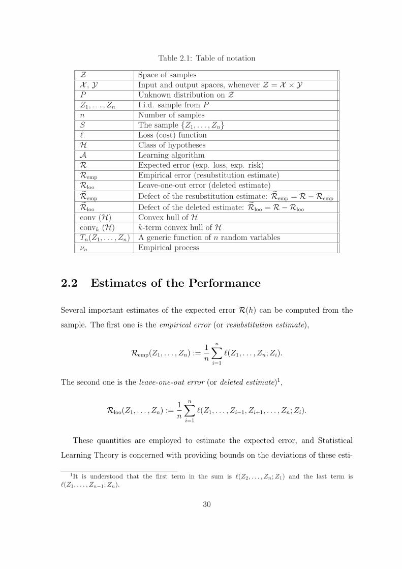
Table 2.1: Table of notation
Z Space of samplesX , Y Input and output spaces, whenever Z = X × YP Unknown distribution on ZZ1, . . . , Zn I.i.d. sample from Pn Number of samplesS The sample Z1, . . . , Zn` Loss (cost) functionH Class of hypothesesA Learning algorithmR Expected error (exp. loss, exp. risk)Remp Empirical error (resubstitution estimate)Rloo Leave-one-out error (deleted estimate)
Remp Defect of the resubstitution estimate: Remp = R−Remp
Rloo Defect of the deleted estimate: Rloo = R−Rloo
conv (H) Convex hull of Hconvk (H) k-term convex hull of HTn(Z1, . . . , Zn) A generic function of n random variablesνn Empirical process
2.2 Estimates of the Performance
Several important estimates of the expected error R(h) can be computed from the
sample. The first one is the empirical error (or resubstitution estimate),
Remp(Z1, . . . , Zn) :=1
n
n∑i=1
`(Z1, . . . , Zn; Zi).
The second one is the leave-one-out error (or deleted estimate)1,
Rloo(Z1, . . . , Zn) :=1
n
n∑i=1
`(Z1, . . . , Zi−1, Zi+1, . . . , Zn; Zi).
These quantities are employed to estimate the expected error, and Statistical
Learning Theory is concerned with providing bounds on the deviations of these esti-
1It is understood that the first term in the sum is `(Z2, . . . , Zn;Z1) and the last term is`(Z1, . . . , Zn−1; Zn).
30

mates from the expected error. For convenience, denote these deviations
Remp(Z1, . . . , Zn) := R(Z1, . . . , Zn)−Remp(Z1, . . . , Zn),
Rloo(Z1, . . . , Zn) := R(Z1, . . . , Zn)−Rloo(Z1, . . . , Zn).
With this notation, Equation 2.1 becomes
P(∣∣∣Remp(Z1, . . . , Zn)
∣∣∣ ≥ ε)
< δ(ε, n) (2.2)
or
P(∣∣∣Rloo(Z1, . . . , Zn)
∣∣∣ ≥ ε)
< δ(ε, n) (2.3)
If one can show that Remp (or Rloo) is “small”, then the empirical error (resp.
leave-one-out error) is a good proxy for the expected error. Hence, a small empirical
(or leave-one-out error) implies a small expected error, with a certain confidence. In
particular, we are often interested in the rate of the convergence of Remp and Rloo to
zero as n increases.
The goal is to derive bounds such that limn→∞ δ(ε, n) = 0 for any fixed ε > 0.
If the rate of decrease of δ(ε, n) is not important, we will write |Remp| P−→ 0 and
|Rloo| P−→ 0.
Let us focus on the random variable Remp(Z1, . . . , Zn). Recall that the Central
Limit Theorem (CLT) guarantees that the average of n i.i.d. random variables con-
verges to their mean (under the assumption of finiteness of second moment) quite
fast. Unfortunately, the random variables
`(Z1, . . . , Zn; Z1), . . . , `(Z1, . . . , Zn; Zn)
are dependent, and the CLT is not applicable. In fact, the interdependence of these
random variables makes the resubstitution estimate positively biased, as the next
example shows.
31

Example 1. Let X = [0, 1], Y = 0, 1, and
P (X) = U [0, 1], P (Y |X) = δY =1.
Suppose `(h(x), y) = I(h(x) 6= y), and A is defined as A(Z1, . . . , Zn; X) = 1 if
X ∈ X1, ..., Xn and 0 otherwise. In other words, the algorithm observes n data
points (Xi, 1), where Xi is distributed uniformly on [0, 1], and generates a hypothesis
which fits exactly the observed data, but outputs 0 for unseen points X. This situation
is depicted in Figure 2-1. The empirical error of A is 0, while the expected error is
1, i.e. Remp(Z1, . . . , Zn) = 1 for any Z1, . . . , Zn.
X1 Xn
0
1
Figure 2-1: Fitting the data.
No guarantee on smallness of Remp can be made in Example 1. Intuitively, this is
due to the fact that the algorithm can fit any data, i.e. the space of functions L(H)
is too large.
Assume that we have no idea what the learning algorithm is except that it picks
its hypotheses from H. To bound Remp, we would need to resort to the worst-
case approach of bounding the deviations between empirical and expected errors for
all functions simultaneously. The ability to make such a statement is completely
characterized by the “size” of L(H), as discussed next.
2.2.1 Uniform Convergence of Means to Expectations
The class L(H) is called uniform Glivenko-Cantelli if for every ε > 0,
32

limn→∞
supµP
(sup
`∈L(H)
∣∣∣∣∣E`− 1
n
n∑i=1
`(Zi)
∣∣∣∣∣ ≥ ε
)= 0,
where Z1, . . . , Zn are i.i.d random variables distributed according to µ.
Non-asymptotic results of the form
P
(sup
`∈L(H)
∣∣∣∣∣E`− 1
n
n∑i=1
`(Zi)
∣∣∣∣∣ ≥ ε
)≤ δ(ε, n,L(H))
give uniform (over the class L(H)) rates of convergence of empirical means to expec-
tations. Since the guarantee is given for all functions in the class, we immediately
obtain
P(∣∣∣Remp(Z1, . . . , Zn)
∣∣∣ ≥ ε)≤ δ(ε, n,L(H)).
We postpone further discussion of Glivenko-Cantelli classes of functions to Section
2.5.
2.2.2 Algorithmic Stability
The uniform-convergence approach above ignores the algorithm, except for the fact
that it picks its hypotheses from H. Hence, this approach might provide only loose
bounds on Remp. Indeed, suppose that the algorithm would in fact only pick one
function from H. The bound on Remp would then follow immediately from The
Central Limit Theorem. It turns out that analogous bounds can be proved even if
the algorithm picks diverse functions, as long is it is done in a “smooth” way. In
Chapter 3, we will derive bounds on both Remp and Rloo in terms of various stability
conditions on the algorithm. Such algorithm-dependent conditions provide guarantees
for Remp and Rloo even when the uniform-convergence approach of Section 2.2.1 fails.
33
2.3 Some Algorithms
2.3.1 Empirical Risk Minimization
The simplest method of learning from observed data is the Empirical Risk Minimiza-
tion (ERM) algorithm
A(Z1, . . . , Zn) = arg minh∈H
1
n
n∑i=1
`(h; Zi).
Note that the ERM algorithm is defined with respect to a class H. Although an
exact minimizer of empirical risk in this class might not exist, an almost-minimizer
always exists. This situation will be discussed in much greater detail in Chapter 5.
The algorithm in Example 1 is an example of ERM over the function class
H =⋃n≥1
hx : x = (x1, . . . , xn) ∈ [0, 1]n,
where hx(x) = 1 if x = xi for some 1 ≤ i ≤ n and hx(x) = 0 otherwise.
ERM over uniform Glivenko-Cantelli classes is a consistent procedure in the sense
that the expected performance converges to the best possible within the class of
hypotheses.
There are a number of drawbacks of ERM: ill-posedness for general classes H, as
well as computational intractability (e.g. for classification with the indicator loss).
The following two families of algorithms, regularization algorithms and boosting algo-
rithms, aim to overcome these difficulties.
2.3.2 Regularization Algorithms
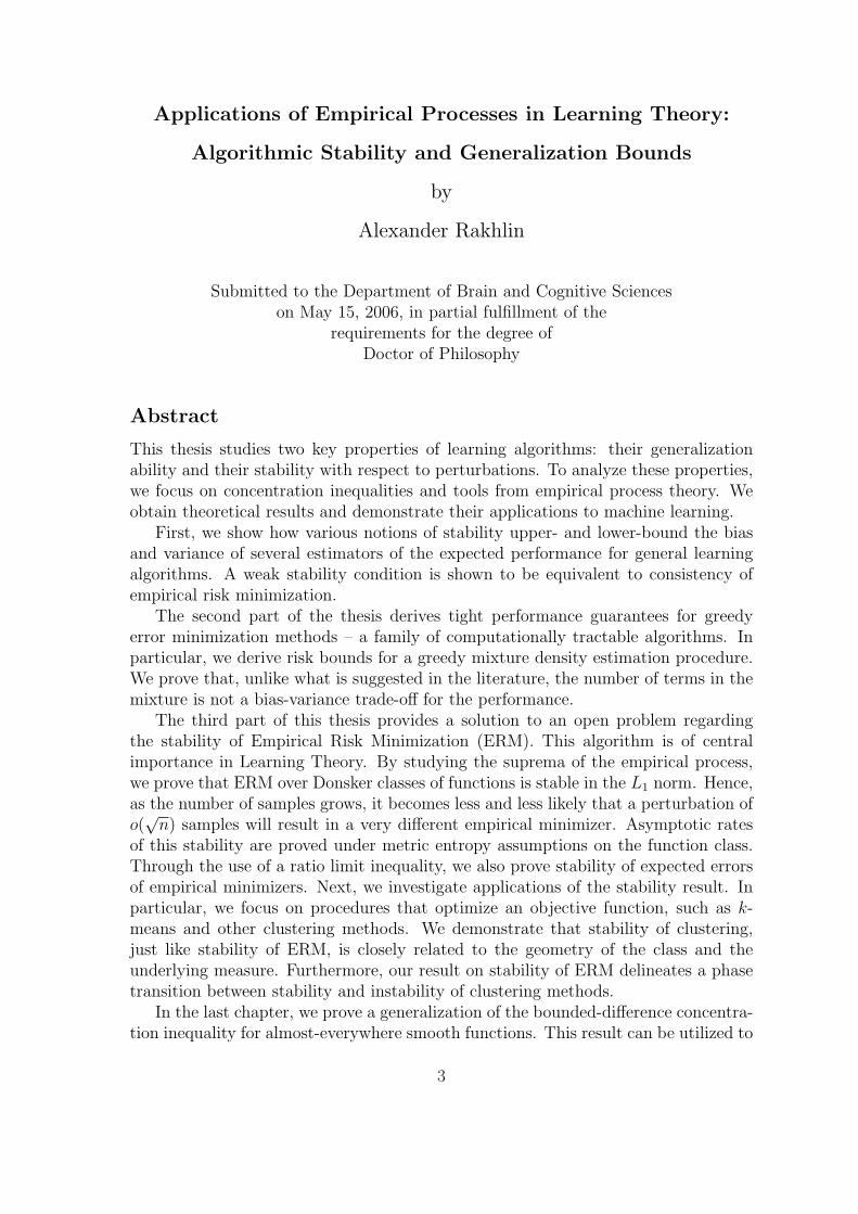
One of the drawbacks of ERM is ill-posedness of the solution. Indeed, learning can be
viewed as reconstruction of the function from the observed data (inverse problem),
and the information contained in the data is not sufficient for the solution to be
unique. For instance, there could be an infinite number of hypotheses with zero
empirical risk, as shown in Figure 2-2. Moreover, the inverse mapping tends to be
34

unstable.
Figure 2-2: Multiple minima of the empirical risk: two dissimilar functions fit thedata.
The regularization method described next is widely used in machine learning
[57, 77], and arises from the theory of solving ill-posed problems. Discovered by
J. Hadamard, ill-posed inverse problems turned out to be important in physics and
statistics (see Chapter 7 of Vapnik [72]).
Let Z = X × Y , i.e. we consider regression or classification. The Tikhonov regu-
larization method [68], applied to the learning setting, proposes to solve the following
minimization problem
A(Z1, . . . , Zn) = arg minh∈H
1
n
n∑i=1
`(h(Xi), Yi) + λ‖h‖2K ,
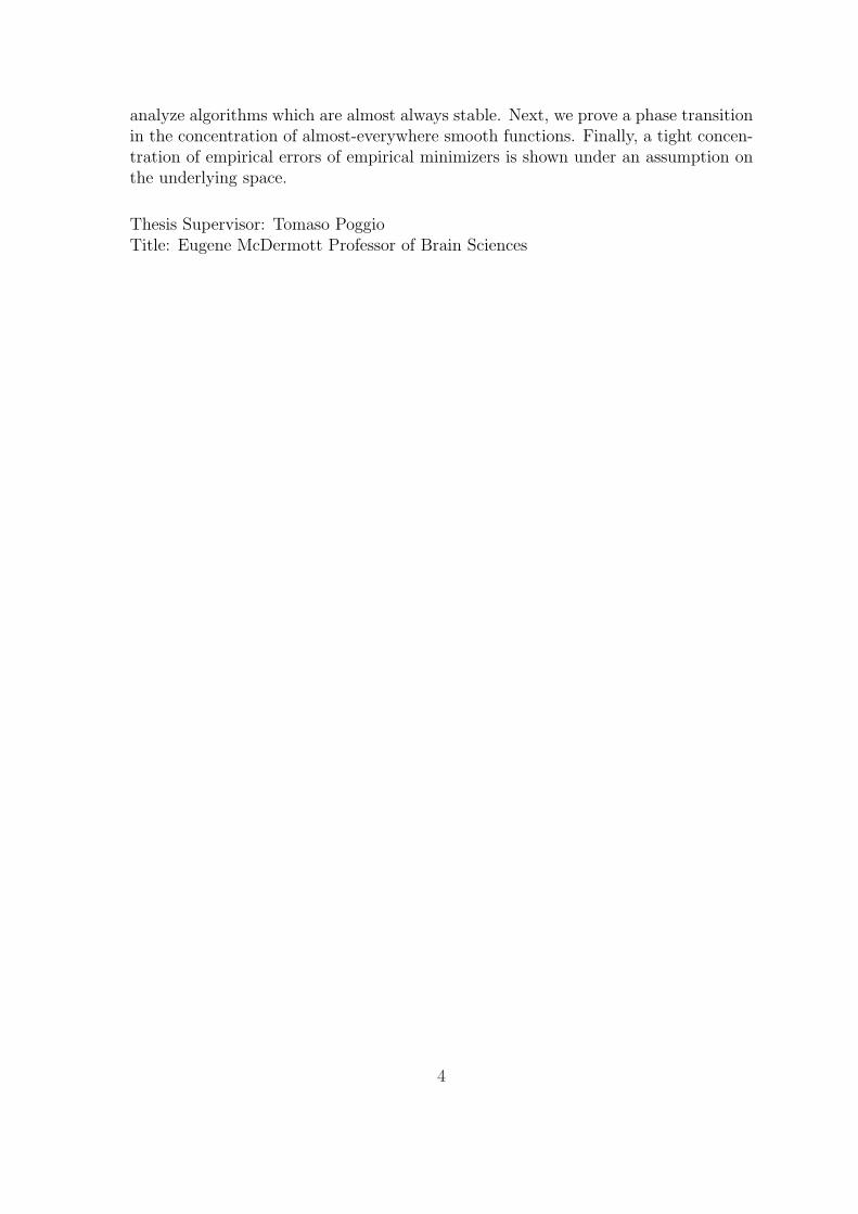
where K is a positive definite kernel and ‖·‖ is the norm in the associated Reproducing
Kernel Hilbert Space H. The parameter λ ≥ 0 controls the balance of the fit to
the data (the first term) and the “smoothness” of the solution (the second term),
and is usually set by a cross-validation method. It is exactly this balance between
smoothness and fit to the data that restores the uniqueness of the solution. It also
restores stability.
This particular minimization problem owes its success to the following surprising
(although simple to prove) fact: even though the minimization is performed over a
possibly infinite-dimensional Hilbert Space of functions, the solution always has the
35
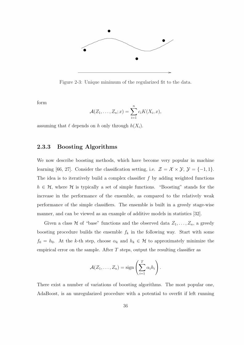
Figure 2-3: Unique minimum of the regularized fit to the data.
form
A(Z1, . . . , Zn; x) =n∑
i=1
ciK(Xi, x),
assuming that ` depends on h only through h(Xi).
2.3.3 Boosting Algorithms
We now describe boosting methods, which have become very popular in machine
learning [66, 27]. Consider the classification setting, i.e. Z = X × Y , Y = −1, 1.The idea is to iteratively build a complex classifier f by adding weighted functions
h ∈ H, where H is typically a set of simple functions. “Boosting” stands for the
increase in the performance of the ensemble, as compared to the relatively weak
performance of the simple classifiers. The ensemble is built in a greedy stage-wise
manner, and can be viewed as an example of additive models in statistics [32].
Given a class H of “base” functions and the observed data Z1, . . . , Zn, a greedy
boosting procedure builds the ensemble fk in the following way. Start with some
f0 = h0. At the k-th step, choose αk and hk ∈ H to approximately minimize the
empirical error on the sample. After T steps, output the resulting classifier as
A(Z1, . . . , Zn) = sign
(T∑
i=1
αihi
).
There exist a number of variations of boosting algorithms. The most popular one,
AdaBoost, is an unregularized procedure with a potential to overfit if left running
36
for enough time. The regularization is performed as a constraint on the norm of the
coefficients or via early stopping. The precise details of a boosting procedure with the
constraint on the `1 norm of the coefficients are given in Chapter 4, where a bound
on the generalization performance is proved.
2.4 Concentration Inequalities
In the context of learning theory, concentration inequalities serve as tools for obtain-
ing generalization bounds. While deviation inequalities are probabilistic statements
about the deviation of a random variable from its expectation, the term “concentra-
tion” often refers to the exponential bounds on the deviation of a function of many
random variables from its mean. The reader is referred to the excellent book of
Ledoux [47] for more information on the concentration of measure phenomenon. The
well-known probabilistic statements mentioned below can be found, for instance, in
the survey by Boucheron et al [13].
Let us start with some basic probability inequalities. For a non-negative random
variable X,
EX =
∫ ∞
0
P (X ≥ t) dt.
The integral above can be lower-bounded by the product tP (X ≥ t) for any fixed
t > 0. Hence, we obtain Markov’s inequality:
P (X > t) ≤ EX
t
for a non-negative random variable X and any t > 0.
For a non-negative strictly monotonically increasing function φ,
P (X ≥ t) = P (φ(X) ≥ φ(t)) ,
resulting in
P (X ≥ t) ≤ Eφ(X)
φ(t)
37

for an arbitrary random variable X.
Setting φ(x) = xq for any q > 0 leads to the method of moments
P (|X − EX| ≥ t) ≤ E |X − EX|qtq
for any random variable X. Since the inequality holds for any q > 0, one can optimize
the bound to get the smallest one. This idea will be used in Chapter 6. Setting
q = 2 we obtain Chebyshev’s inequality which uses the second-moment information
to bound the deviation of X from its expectation:
P (|X − EX| ≥ t) ≤ VarX
t2.
Other choices of φ lead to useful probability inequalities. For instance, φ(x) = esx
for s > 0 leads to the Chernoff’s bounding method. Since
P (X ≥ t) = P(esX ≥ est
),
we obtain
P (X ≥ t) ≤ EesX
est.
Once some information about X is available, one can minimize the above bound over
s > 0.
So far, we have discussed generic probability inequalities which do not exploit any
“structure” of X. Suppose X is in fact a function of n random variables. Instead of
the letter X, let us denote the function of n random variables by Tn(Z1, . . . , Zn).
Theorem 2.4.1 (Hoeffding [34]). Suppose Tn(Z1, . . . , Zn) =∑n
i=1 Zi, where Zi’s are
independent and ai ≤ Zi ≤ bi. Then for any ε > 0,
P (|Tn − ETn| > ε) ≤ 2e−2ε2Pn
i=1(bi−ai)
2
Hoeffding’s inequality does not use any information about the variances of Zi’s.
A tighter bound can be obtained whenever these variances are small.
38

Theorem 2.4.2 (Bennett [10]). Suppose Tn(Z1, . . . , Zn) =∑n
i=1 Zi, where Zi’s are
independent, and for any i, EZi = 0 and |Zi| ≤ M . Let σ2 = 1n
∑ni=1 VarZi. Then
for any ε > 0,
P (|Tn| > ε) ≤ 2 exp
(−nσ2
M2φ
(εM
nσ2
)),
where φ(x) = (1 + x) log(1 + x)− x.
Somewhat surprisingly, exponential deviation inequalities hold not only for sums,
but for general “smooth” functions of n variables.
Theorem 2.4.3 (McDiarmid [54]). Let Tn : Zn → R such that
∀z1, . . . , zn, z′1, . . . , z′n ∈ Z |Tn(z1, . . . , zn)− Tn(z1, . . . , z
′i, . . . , zn)| ≤ ci.
Let Z1, . . . , Zn be independent random variables. Then
P (Tn(Z1, . . . , Zn)− ETn(Z1, . . . , Zn) > ε) ≤ exp
(− ε2
2∑n
i=1 c2i
)
and
P (Tn(Z1, . . . , Zn)− ETn(Z1, . . . , Zn) < −ε) ≤ exp
(− ε2
2∑n
i=1 c2i
).
The following Efron-Stein’s inequality can be used to directly upper-bound the
variance of functions of n random variables.
Theorem 2.4.4 (Efron-Stein [26]). Let Tn : Zn 7→ R be a measurable function of n
variables and define Γ = Tn(Z1, . . . , Zn) and Γ′i = Tn(Z1, . . . , Z′i, . . . , Zn), where
Z1, . . . , Zn, Z′1, . . . , Z
′n
are i.i.d. random variables. Then
Var(Tn) ≤ 1
2
n∑i=1
E[(Γ− Γ′i)
2]. (2.4)
A “removal” version of the above is the following:
39
Theorem 2.4.5 (Efron-Stein). Let Tn : Zn 7→ R be a measurable function of n
variables and T ′n : Zn−1 7→ R of n − 1 variables. Define Γ = Tn(Z1, . . . , Zn) and
Γi = T ′n(Z1, . . . , Zi−1, Zi+1, . . . , Zn), where Z1, . . . , Zn are i.i.d. random variables.
Then
Var(Tn) ≤n∑
i=1
E[(Γ− Γi)
2]. (2.5)
A collection of random functions Tn for n = 1, 2, . . . can be viewed as a sequence
of random variables Tn. There are several important notions of convergence of
sequences of random variables: in probability and almost surely.
Definition 2.4.1. A sequence Tn, n = 1, 2, . . ., of random variables converges to
T in probability
TnP−→ T
if for each ε > 0
limn→∞
P (|Tn − T | ≥ ε) = 0.
This can also be written as
P (|Tn − T | ≥ ε) → 0.
Definition 2.4.2. A sequence Tn, n = 1, 2, . . ., of random variables converges to
T almost surely if
P(
limn→∞
Tn = T)
= 0.
Deviation inequalities provide specific upper bounds on the convergence of
P (|Tn − T | ≥ ε) → 0.
Assume for simplicity that Tn is a non-negative function and the limit T is 0. When
inspecting inequalities of the type
P (Tn ≥ ε) ≤ δ(ε, n)
40
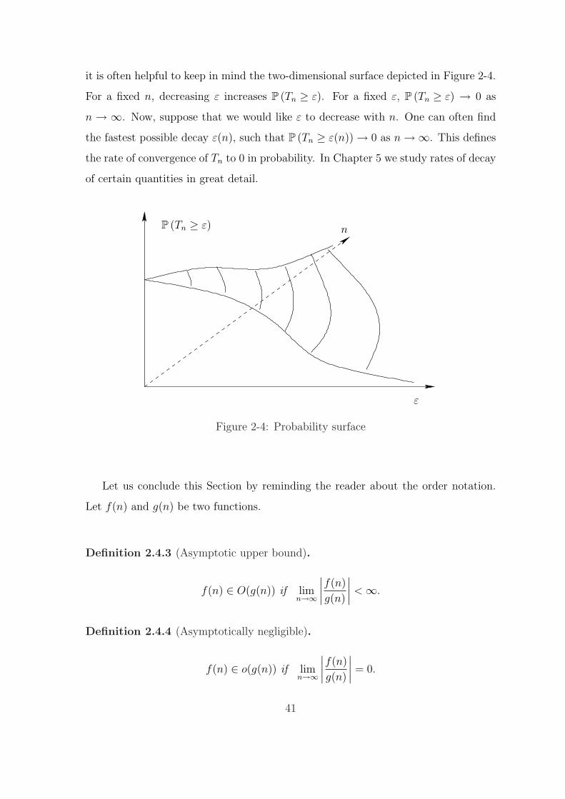
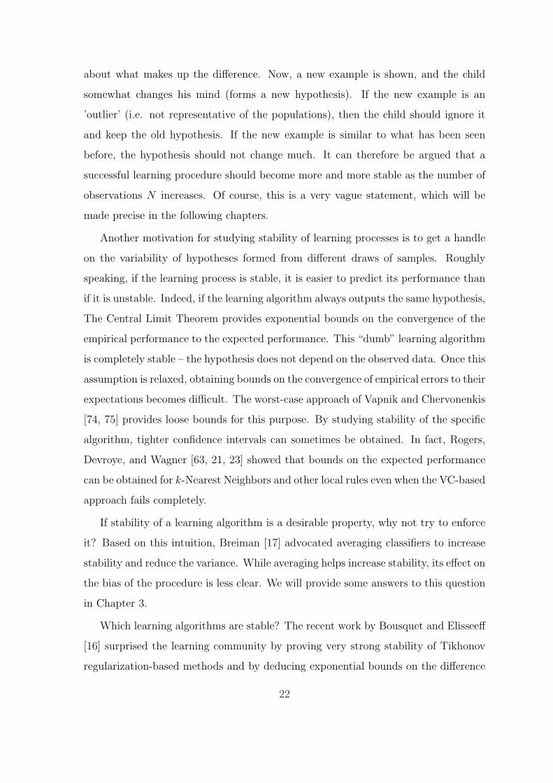
it is often helpful to keep in mind the two-dimensional surface depicted in Figure 2-4.
For a fixed n, decreasing ε increases P (Tn ≥ ε). For a fixed ε, P (Tn ≥ ε) → 0 as
n → ∞. Now, suppose that we would like ε to decrease with n. One can often find
the fastest possible decay ε(n), such that P (Tn ≥ ε(n)) → 0 as n →∞. This defines
the rate of convergence of Tn to 0 in probability. In Chapter 5 we study rates of decay
of certain quantities in great detail.
ε
nP (Tn ≥ ε)
Figure 2-4: Probability surface
Let us conclude this Section by reminding the reader about the order notation.
Let f(n) and g(n) be two functions.
Definition 2.4.3 (Asymptotic upper bound).
f(n) ∈ O(g(n)) if limn→∞
∣∣∣∣f(n)
g(n)
∣∣∣∣ < ∞.
Definition 2.4.4 (Asymptotically negligible).
f(n) ∈ o(g(n)) if limn→∞
∣∣∣∣f(n)
g(n)
∣∣∣∣ = 0.
41

Definition 2.4.5 (Asymptotic lower bound).
f(n) ∈ Ω(g(n)) if limn→∞
∣∣∣∣f(n)
g(n)
∣∣∣∣ > 0.
In the above definitions, “∈” will often be replaced by “=”.
2.5 Empirical Process Theory
In this section, we briefly mention a few results from the Theory of Empirical Pro-
cesses, relevant to this thesis. The reader is referred to the excellent book by A. W.
van der Waart and J. A. Wellner [71].
2.5.1 Covering and Packing Numbers
Fix a distance function d(f, g) for f, g ∈ H.
Definition 2.5.1. Given ε > 0 and h1, . . . , hN ∈ H, we say that h1, . . . , hN are
ε-separated if d(hi, hj) > ε for any i 6= j.
The ε-packing number, D(H, ε, d), is the maximal cardinality of an ε-separated
set.
Definition 2.5.2. Given ε > 0 and h1, . . . , hN ∈ H, we say that the set h1, . . . , hN
is an ε-cover of H if for any h ∈ H, there exists 1 ≤ i ≤ N such that d(h, hi) ≤ ε.
The ε-covering number, N (H, ε, d), is the minimal cardinality of an ε-cover of H.
Furthermore, logN (H, ε, d) is called metric entropy.
It can be shown that
D(H, 2ε, d) ≤ N (H, ε, d) ≤ D(H, ε, d).
Definition 2.5.3. Entropy with bracketing N[](H, ε, d) is defined as the smallest num-
ber N for which there exists pairs hi, h′iN
i=1 such that d(hi, h′i) ≤ ε for all i and for
any h ∈ H there exists a pair hj, h′j such that hj ≤ h ≤ h′j.
42

2.5.2 Donsker and Glivenko-Cantelli Classes
Let Pn stand for the discrete measure supported on Z1, . . . , Zn. More precisely,
Pn =1
n
n∑i=1
δZi,
the sum of Dirac measures at the samples. Throughout this thesis, we will denote
Pf = EZf(Z) and Pnf =1
n
n∑i=1
f(Zi).
Define the sup norm as
‖Qf‖F = supf∈F
|Qf |
for any measure Q.
We now introduce the notion of empirical process.
Definition 2.5.4. The empirical process νn indexed by a function class F is defined
as the map
f 7→ νn(f) =√
n(Pn − P )f =1√n
n∑i=1
(f(Zi)− Pf).
The Law of Large Numbers (LLN) guarantees that Pnf converges to Pf for a
fixed f , if the latter exists. Moreover, the Central Limit Theorem (CLT) guaran-
tees that the empirical process νn(f) converges to N(0, P (f − Pf)2) if Pf 2 is finite.
Similar statements can be made for a finite number of functions simultaneously. The
analogous statements that hold uniformly over infinite function classes are the core
topic of Empirical Process Theory.
Definition 2.5.5. A class F is called P -Glivenko-Cantelli if
‖Pn − P‖F P ∗−→ 0,
where the convergence is in (outer) probability or (outer) almost surely [71].
43

Definition 2.5.6. A class F is called P -Donsker if
νn à ν
in `∞(F), where the limit ν is a tight Borel measurable element in `∞(F) and “ Ã′′
denotes weak convergence, as defined on p. 17 of [71].
In fact, it follows that the limit process ν must be a zero-mean Gaussian process
with covariance function Eν(f)ν(f ′) = 〈f, f ′〉 (i.e. a Brownian bridge).
While Glivenko-Cantelli classes of functions have been used in Learning Theory
to a great extent, the important properties of Donsker classes have not been utilized.
In Chapter 5, P -Donsker classes of functions play an important role because of a
specific covariance structure they possess. We hypothesize that many more results
can be discovered for learning with Donsker classes.
Various Donsker theorems provide sufficient conditions for a class being P -Donsker.
Here we mention a few known results (see [71], Eqn. 2.1.7 and [70], Thm. 6.3) in
terms of entropy logN and entropy with bracketing logN[].
Proposition 2.5.1. If the envelope F of F is square integrable and
∫ ∞
0
supQ
√logN (ε ‖F‖Q,2 ,F , L2(Q))dε < ∞,
then F is P -Donsker for every P , i.e. F is a universal Donsker class. Here the
supremum is taken over all finitely discrete probability measures.
Proposition 2.5.2. If∫∞
0
√logN[](ε,F , L2(P ))dε < ∞, then F is P -Donsker.
From the learning theory perspective, however, the most interesting theorems are
probably those relating the Donsker property to the VC-dimension. For example, if Fis a 0, 1-valued class, then F is universal Donsker if and only if its VC dimension is
finite (Thm. 10.1.4 of [25] provides a more general result involving Pollard’s entropy
condition). As a corollary of their Proposition 3.1, [29] show that under the Pollard’s
entropy condition, the 0, 1-valued class F is in fact uniform Donsker. Finally,
44
Rudelson and Vershynin [64] extended these results to the real-valued case: a class
F is uniform Donsker if the square root of its VC dimension is integrable.
2.5.3 Symmetrization and Concentration
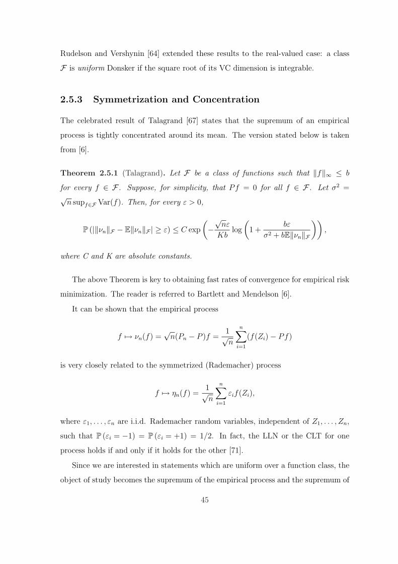
The celebrated result of Talagrand [67] states that the supremum of an empirical
process is tightly concentrated around its mean. The version stated below is taken
from [6].
Theorem 2.5.1 (Talagrand). Let F be a class of functions such that ‖f‖∞ ≤ b
for every f ∈ F . Suppose, for simplicity, that Pf = 0 for all f ∈ F . Let σ2 =√
n supf∈F Var(f). Then, for every ε > 0,
P (|‖νn‖F − E‖νn‖F | ≥ ε) ≤ C exp
(−√
nε
Kblog
(1 +
bε
σ2 + bE‖νn‖F
)),
where C and K are absolute constants.
The above Theorem is key to obtaining fast rates of convergence for empirical risk
minimization. The reader is referred to Bartlett and Mendelson [6].
It can be shown that the empirical process
f 7→ νn(f) =√
n(Pn − P )f =1√n
n∑i=1
(f(Zi)− Pf)
is very closely related to the symmetrized (Rademacher) process
f 7→ ηn(f) =1√n
n∑i=1
εif(Zi),
where ε1, . . . , εn are i.i.d. Rademacher random variables, independent of Z1, . . . , Zn,
such that P (εi = −1) = P (εi = +1) = 1/2. In fact, the LLN or the CLT for one
process holds if and only if it holds for the other [71].
Since we are interested in statements which are uniform over a function class, the
object of study becomes the supremum of the empirical process and the supremum of
45
the Rademacher process. The Symmetrization technique [28] is key to relating these
two.
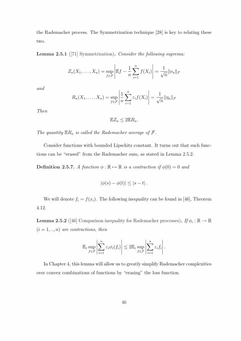
Lemma 2.5.1 ([71] Symmetrization). Consider the following suprema:
Zn(X1, . . . , Xn) = supf∈F
∣∣∣∣∣Ef − 1
n
n∑i=1
f(Xi)
∣∣∣∣∣ =1√n‖νn‖F
and
Rn(X1, . . . , Xn) = supf∈F
∣∣∣∣∣1
n
n∑i=1
εif(Xi)
∣∣∣∣∣ =1√n‖ηn‖F
Then
EZn ≤ 2ERn.
The quantity ERn is called the Rademacher average of F .
Consider functions with bounded Lipschitz constant. It turns out that such func-
tions can be “erased” from the Rademacher sum, as stated in Lemma 2.5.2.
Definition 2.5.7. A function φ : R 7→ R is a contraction if φ(0) = 0 and
|φ(s)− φ(t)| ≤ |s− t| .
We will denote fi = f(xi). The following inequality can be found in [46], Theorem
4.12.
Lemma 2.5.2 ([46] Comparison inequality for Rademacher processes). If φi : R→ R
(i = 1, .., n) are contractions, then
Eε supf∈F
∣∣∣∣∣n∑
i=1
εiφi(fi)
∣∣∣∣∣ ≤ 2Eε supf∈F
∣∣∣∣∣n∑
i=1
εifi
∣∣∣∣∣ .
In Chapter 4, this lemma will allow us to greatly simplify Rademacher complexities
over convex combinations of functions by “erasing” the loss function.
46

Chapter 3
Generalization Bounds via
Stability
The results of this Chapter appear in [60].
3.1 Introduction
Albeit interesting from the theoretical point of view, the uniform bounds, discussed
in Section 2.2.1, are, in general, loose, as they are worst-case over all functions in the
class. As an extreme example, consider the algorithm that always ouputs the same
function (the constant algorithm)
A(Z1, . . . , Zn) = f0, ∀(Z1, . . . , Zn) ∈ Zn.
The bound on Remp(Z1, . . . , Zn) follows from the CLT and an analysis based upon
the complexity of a class H does not make sense.
Recall from the previous Chapter that we would like, for a given algorithm, to
obtain the following generalization bounds
P(∣∣∣Remp(Z1, . . . , Zn)
∣∣∣ > ε)
< δ(ε, n) or P(∣∣∣Rloo(Z1, . . . , Zn)
∣∣∣ > ε)
< δ(ε, n)
47

with δ(ε, n) → 0 as n →∞.
Throughout this Chapter, we assume that the loss function ` is bounded and non-
negative, i.e. 0 ≤ ` ≤ M . Notice that Remp and Rloo are bounded random variables.
By Markov’s inequality,
∀ε ≥ 0, P(|Remp| ≥ ε
)≤ E|Remp|
ε
and also
∀ε′ ≥ 0, E|Remp| ≤ MP(|Remp| ≥ ε′
)+ ε′.
Therefore, showing
|Remp| P−→ 0
is equivalent to showing
E|Remp| → 0.
The latter is equivalent to
E(Remp)2 → 0
since |Remp| ≤ M . Further notice that
E(Remp)2 = Var(Remp) + (ERemp)
2.
We will call ERemp the bias, Var(Remp) the variance, and E(Remp)2 the second mo-
ment of Remp. The same derivations and terminology hold for Rloo.
Hence, studying conditions for convergence in probability of the estimators to zero
is equivalent to studying their mean and variance (or the second moment alone).
In this Chapter we consider various stability conditions which allow one to bound
bias and variance or the second moment, and thus imply convergence of Remp and
Rloo to zero in probability. Though the reader should expect a number of definitions
of stability, the common flavor of these notions is the comparison of the “behavior”
of the algorithm A on similar samples. We hope that the present work sheds light
on the important stability aspects of algorithms, suggesting principles for designing
48

predictive learning systems.
We now sketch the organization of this Chapter. In Section 3.2 we motivate
the use of stability and give some historical background. In Section 3.3, we show
how bias (Section 3.3.1) and variance (Section 3.3.2) can be bounded by various
stability quantities. Sometimes it is mathematically more convenient to bound the
second moment instead of bias and variance, and this is done in Section 3.4. In
particular, Section 3.4.1 deals with the second moment E(Rloo)2 in the spirit of [22],
while in Sections 3.4.3 and 3.4.2 we bound E(Remp)2 in the spirit of [55] and [16],
respectively. The goal of Sections 3.4.1 and 3.4.2 is to re-derive some known results
in a simple manner that allows one to compare the proofs side-by-side. The results
of these sections hold for general algorithms. Furthermore, for specific algorithms
the results can be improved, i.e. simpler quantities might govern the convergence
of the estimators to zero. To illustrate this, in Section 3.4.4 we prove that for the
empirical risk minimization algorithm, a bound on the bias ERemp implies a bound on
the second moment E(Remp)2. We therefore provide a simple necessary and sufficient
condition for consistency of ERM. If rates of convergence are of importance, rather
than using Markov’s inequality, one can make use of more sophisticated concentration
inequalities with a cost of requiring more stringent stability conditions. In Section
3.6, we discuss the most rigid stability, Uniform Stability, and provide exponential
bounds in the spirit of [16]. In Section 3.6.2 we consider less rigid notions of stability
and prove exponential inequalities based on powerful moment inequalities of [15].
Finally, Section 3.7 summarizes the Chapter and discusses further directions and
open questions.
3.2 Historical Remarks and Motivation
Devroye, Rogers, and Wagner (see e.g. [22]) were the first, to our knowledge, to
observe that the sensitivity of the algorithms with regard to small changes in the
sample is related to the behavior of the leave-one-out estimate. The authors were
able to obtain results for the k-Nearest-Neighbor algorithm, where VC theory fails
49
because of large class of potential hypotheses. These results were further extended
for k-local algorithms and for potential learning rules. Kearns and Ron [36] later
discovered a connection between finite VC-dimension and stability. Bousquet and
Elisseeff [16] showed that a large class of learning algorithms, based on Tikhonov
Regularization, is stable in a very strong sense, which allowed the authors to obtain
exponential generalization bounds. Kutin and Niyogi [44] introduced a number of
notions of stability and showed implications between them. The authors emphasized
the importance of “almost-everywhere” stability and proved valuable extensions of
McDiarmid’s exponential inequality [43]. Mukherjee et al [55] proved that a com-
bination of three stability notions is sufficient to bound the difference between the
empirical estimate and the expected error, while for empirical risk minimization these
notions are necessary and sufficient. The latter result showed an alternative to VC
theory condition for consistency of empirical risk minimization. In this Chapter we
prove, in a unified framework, some of the important results mentioned above, as well
as show new ways of incorporating stability notions in Learning Theory.
We now give some intuition for using algorithmic stability. First, note that without
any assumptions on the algorithm, nothing can be said about the mean and the
variance of Remp. One can easily come up with settings when the mean is converging
to zero, but not the variance, or vice versa (e.g. Example 1), or both quantities
diverge from zero.
The assumptions of this Chapter that allow us to bound the mean and the variance
of Remp and Rloo are loosely termed as stability assumptions. Recall that if the
algorithm is a constant algorithm, Remp is bounded by the Central Limit Theorem.
Of course, this is an extreme and the most “stable” case. It turns out that the
“constancy” assumption on the algorithm can be relaxed while still achieving tight
bounds. A central notion here is that of Uniform Stability [16]:
Definition 3.2.1. Uniform Stability β∞(n) of an algorithm A is
β∞(n) := supZ1,...,Zn,z∈Z,x∈X
|A(Z1, . . . , Zn; X)−A(z, Z2, . . . , Zn; X)|.
50
Intuitively, if β∞(n) → 0, the algorithm resembles more and more the constant
algorithm when considered on similar samples (although it can produce distant func-
tions on different samples). It can be shown that some well-known algorithms possess
Uniform Stability with a certain rate on β∞(n) (see [16] and section 3.6.1).
In the following sections, we will show how the bias and variance (or second
moment) can be upper-bounded or decomposed in terms of quantities over “similar”
samples. The advantage of this approach is that it allows one to check stability for a
specific algorithm and derive generalization bounds without much further work. For
instance, it is easy to show that k-Nearest Neighbors algorithm is L1-stable and a
generalization bound follows immediately (see section 3.4.1).
3.3 Bounding Bias and Variance
3.3.1 Decomposing the Bias
The bias of the resubstitution estimate and the deleted estimate can be written as
quantities over similar samples:
ERemp = E
[1
n
n∑i=1
[Ez`(Z1, . . . , Zn; Z)− `(Z1, . . . , Zn; Zi)]
]
= E [`(Z1, . . . , Zn; Z)− `(Z1, . . . , Zn; Z1)]
= E [`(Z,Z2, . . . , Zn; Z1)− `(Z1, . . . , Zn; Z1)] .
The first equality above follows because
E`(Z1, . . . , Zn; Zk) = E`(Z1, . . . , Zn; Zm)
for any k, m. The second equality holds by noticing that
E`(Z1, . . . , Zn; Z) = E`(Z, Z2, . . . , Zn; Z1)
51

because the roles of Z and Z1 can be switched (see [63]). We will employ this trick
many times in the later proofs, and for convenience we shall denote this renaming
process by Z ↔ Z1.
Let us inspect the quantity
E [`(Z,Z2, . . . , Zn; Z1)− `(Z1, . . . , Zn; Z1)] .
It is the average difference between the loss at a point Z1 when it is not present in the
learning sample (out-of-sample) and the loss at Z1 when it is present in the n-tuple
(in-sample). Hence, the bias ERemp will decrease if and only if the average behavior
on in-sample and out-of-sample points is becoming more and more similar. This is a
stability property and we will give a name to it:
Definition 3.3.1. Average Stability βbias(n) of an algorithm A is
βbias(n) := E [`(Z, Z2, . . . , Zn; Z1)− `(Z1, . . . , Zn; Z1)] .
We now turn to the deleted estimate. The bias ERloo can be written as
ERloo = E
[1
n
n∑i=1
(EZ`(Z1, . . . , Zn; Z)− `(Z1, . . . , Zi−1, Zi+1, . . . , Zn; Zi))
]
= E [`(Z1, . . . , Zn; Z)− `(Z2, . . . , Zn; Z1)]
= E [R(Z1, . . . , Zn)−R(Z2, . . . , Zn)]
We will not give a name to this quantity, as it will not be used explicitly later. One
can see that the bias of the deleted estimate should be small for reasonable algorithms.
Unfortunately, the variance of the deleted estimate is large in general (see e.g. page
415 of [20]). The opposite is believed to be true for the resubstitution estimate. We
refer the reader to Chap. 23, 24, and 31 of [20] for more information. Surprisingly,
we will show in section 3.4.4 that for empirical risk minimization algorithms, if one
shows that the bias of the resubstitution estimate decreases, one also obtains that the
variance decreases.
52

3.3.2 Bounding the Variance
Having shown a decomposition of the bias of Remp and Rloo in terms of stability
conditions, we now show a simple way to bound the variance in terms of quantities
over “similar” samples. In order to upper-bound the variance, we will use the Efron-
Stein’s bounds (Theorems 2.4 and 2.5).
The proofs of the Efron-Stein bounds are based on the fact that
Var(Γ) ≤ E(Γ− c)2
for any constant c, and so
Vari(Γ) = Ezi(Γ− Ezi
Γ)2 ≤ Ezi(Γ− Γi)
2.
Thus, we artificially introduce a quantity over a “similar” sample to upper-bound the
variance. If the increments Γ− Γi and Γ− Γ′i are small, the variance is small. When
applied to the function Tn = Remp(Z1, . . . , Zn), this translates exactly into controlling
the behavior of the algorithm A on similar samples:
Var(Remp) ≤ nE(Remp(Z1, . . . , Zn)− Remp(Z2, . . . , Zn))2
≤ 2nE (R(Z1, . . . , Zn)−R(Z2, . . . , Zn))2
+ 2nE (Remp(Z2, . . . , Zn)−Remp(Z1, . . . , Zn))2 (3.1)
Here we used the fact that the algorithm is invariant under permutation of coor-
dinates, and therefore all the terms in the sum of Equation (2.5) are equal. This
symmetry will be exploited to a great extent in the later sections. Note that similar
results can be obtained using the replacement version of Efron-Stein’s bound.
The meaning of the above bound is that if the mean square of the difference
between expected errors of functions, learned from samples differing in one point, is
decreasing faster than n−1, and if the same holds for the empirical errors, then the
variance of the resubstitution estimate is decreasing. Let us give names to the above
53
quantities.
Definition 3.3.2. Empirical-Error (Removal) Stability of an algorithm A is
β2emp(n) := E |Remp(Z1, . . . , Zn)−Remp(Z1, . . . , Zi−1, Zi+1, . . . , Zn)|2 .
Definition 3.3.3. Expected-Error (Removal) Stability of an algorithm A is
β2exp(n) := E |R(Z1, . . . , Zn)−R(Z1, . . . , Zi−1, Zi+1, . . . , Zn)|2 .
With the above definitions, the following Theorem follows:
Theorem 3.3.1.
Var(Remp) ≤ 2n(β2exp(n) + β2
emp(n)).
The following example shows that the ERM algorithm is always Empirical-Error
Stable with βemp(n) ≤ M(n − 1)−1. We deduce that RempP−→ 0 for ERM whenever
βexp = o(n−1/2). As we will show in Section 3.4.4, the decay of Average Stability,
βbias(n) = o(1), is both necessary and sufficient for RempP−→ 0 for ERM.
Example 2. For an empirical risk minimization algorithm, βemp(n) ≤ Mn−1
:
Remp(Z2, . . . , Zn)−Remp(Z1, . . . , Zn) ≤
≤ 1
n− 1
n∑i=2
`(Z2, . . . , Zn; Zi) − 1
n− 1
n∑i=1
`(Z1, . . . , Zn; Zi) +M
n− 1
≤ 1
n− 1
n∑i=2
`(Z2, . . . , Zn; Zi) − 1
n− 1
n∑i=2
`(Z1, . . . , Zn; Zi)
+M
n− 1− 1
n− 1`(Z1, . . . , Zn; Z1) ≤ M
n− 1
and the other direction is proved similarly.
We will show in the following sections that a direct study of the second moment
leads to better bounds. For the bound on the variance in Theorem 3.3.1 to decrease,
βexp and βemp have to be o(n−1/2). With an additional assumption, we will be able to
54

remove the factor n from the bound 3.1 by upper-bounding the second moment and
by exploiting the structure of the random variables Rloo and Remp.
3.4 Bounding the 2nd Moment
Instead of bounding the mean and variance of the estimators, we can bound the
second moment. The reason for doing so is mathematical convenience and is due to
the following straight-forward bounds on the second moment:
E(Remp)2 = E [EZ`(Z1, . . . , Zn; Z)]2 − E
[EZ`(Z1, . . . , Zn; Z)
1
n
n∑i=1
`(Z1, . . . , Zn; Zi)
]
+ E
[1
n
n∑i=1
`(Z1, . . . , Zn; Zi)
]2
− E[Ez`(Z1, . . . , Zn; Z)
1
n
n∑i=1
`(Z1, . . . , Zn; Zi)
]
≤ E [Ez`(Z1, . . . , Zn; Z)EZ′`(Z1, . . . , Zn; Z ′)− EZ`(Z1, . . . , Zn; Z)`(Z1, . . . , Zn; Z1)]
+ E [`(Z1, . . . , Zn; Z1)`(Z1, . . . , Zn; Z2)− EZ`(Z1, . . . , Zn; Z)`(Z1, . . . , Zn; Z1)]
+1
nE`(Z1, . . . , Zn; Z1)
2,
and the last term is bounded by M2
n. Similarly,
E(Rloo)2 ≤ E [EZ`(Z1, . . . , Zn; Z)EZ′`(Z1, . . . , Zn; Z ′)− EZ`(Z1, . . . , Zn; Z)`(Z2, . . . , Zn; Z1)]
+ E [`(Z2, . . . , Zn; Z1)`(Z1, Z3, · · · , Zn; Z2)− Ez`(Z1, . . . , Zn; Z)`(Z2, . . . , Zn; Z1)]
+1
nE`(Z2, . . . , Zn; Z1)
2,
and the last term is bounded by M2
n.
In the proofs we will use the following inequality for random variables X, X ′ and
Y :
E [XY −X ′Y ] ≤ ME|X −X ′| (3.2)
if −M ≤ Y ≤ M . The bounds on the second moments are already sums of terms of
the type “E [XY −WZ]”, and we will find a way to use symmetry to change these
55

terms into the type “E [XY −X ′Y ]”, where X and X ′ will be quantities over similar
samples, and so E|X −X ′| will be bounded by a certain stability of the algorithm.
3.4.1 Leave-one-out (Deleted) Estimate
We have seen that
ERloo = E [R(Z1, . . . , Zn)−R(Z2, . . . , Zn)]
and thus the bias decreases if and only if the expected errors are similar when learning
on similar (one additional point) samples. Moreover, intuitively, these errors have
to occur at the same places because otherwise evaluation of leave-one-out functions
`(Z1, . . . , Zi−1, Zi+1, . . . , Zn; Z) will not tell us about `(Z1, . . . , Zn; Z). This implies
that the L1 distance between the functions on similar (one additional point) samples
should be small. This connection between L1 stability and the leave-one-out estimate
has been observed by Devroye and Wagner [22] and further studied in [36]. We now
define this stability notion:
Definition 3.4.1. L1-Stability of an algorithm A is
β1(n) : = ‖`(Z1, . . . , Zn; ·)− `(Z2, . . . , Zn; ·)‖L1(µ)
= EZ |`(Z1, . . . , Zn; Z)− `(Z2, . . . , Zn; Z)| .
The following Theorem is proved in [22, 20] for classification algorithms. We give
a similar proof for general learning algorithms. The result shows that the second
moment (and therefore both bias and variance) of the leave-one-out error estimate is
bounded by the L1 distance between loss functions on similar samples.
Theorem 3.4.1.
E(Rloo)2 ≤ M(2β1(n− 1) + 4β1(n)) +
M2
n.
Proof. The first term in the decomposition of the second moment of E(Rloo)2 can be
56

bounded as follows:
E [`(Z1, . . . , Zn; Z)`(Z1, . . . , Zn; Z ′)− `(Z1, . . . , Zn; Z)`(Z2, . . . , Zn; Z1)]
= E [`(Z1, . . . , Zn; Z)`(Z1, . . . , Zn; Z ′)− `(Z ′, Z2, . . . , Zn; Z)`(Z2, . . . , Zn; Z ′)]
= E [`(Z1, . . . , Zn; Z)`(Z1, . . . , Zn; Z ′)− `(Z2, . . . , Zn; Z)`(Z1, . . . , Zn; Z ′)]
+ E [`(Z2, . . . , Zn; Z)`(Z1, . . . , Zn; Z ′)− `(Z ′, Z2, . . . , Zn; Z)`(Z1, . . . , Zn; Z ′)]
+ E [`(Z ′, Z2, . . . , Zn; Z)`(Z1, . . . , Zn; Z ′)− `(z′, Z2, . . . , Zn; Z)`(Z2, . . . , Zn; Z ′)]
≤ 3Mβ1(n).
The first equality holds by renaming Z ′ ↔ Z1. In doing this, we are using the fact
that all the variables Z1, . . . , Zn, Z, Z ′ are identically distributed and independent.
To obtain the inequality above, note that each of the three terms is bounded (using
Ineq. 3.2) by Mβ1(n) .
The second term in the decomposition is bounded similarly:
E [`(Z2, . . . , Zn; Z1)`(Z1, Z3, . . . , Zn; Z2)− `(Z1, . . . , Zn; Z)`(Z2, . . . , Zn; Z1)]
= E [`(Z ′, Z3, . . . , Zn; Z)`(Z, Z3, . . . , Zn; Z ′)− `(Z ′, Z2, . . . , Zn; Z)`(Z2, . . . , Zn; Z ′)]
= E [`(Z ′, Z3, . . . , Zn; Z)`(Z, Z3, . . . , Zn; Z ′)− `(Z ′, Z2, . . . , Zn; Z)`(Z,Z3, . . . , Zn; Z ′)]
+ E [`(Z ′, Z2, . . . , Zn; Z)`(Z, Z3, . . . , Zn; Z ′)− `(Z ′, Z2, . . . , Zn; Z)`(Z3, . . . , Zn; Z ′)]
+ E [`(Z ′, Z2, . . . , Zn; Z)`(Z3, . . . , Zn; Z ′)− `(Z ′, Z2, . . . , Zn; Z)`(Z2, . . . , Zn; Z ′)]
≤ Mβ1(n) + 2Mβ1(n− 1)
The first equality follows by renaming Z2 ↔ Z ′ as well as Z1 ↔ Z in the first term,
and Z1 ↔ Z ′ in the second term. Finally, we bound the last term by M2/n to obtain
the result.
57

3.4.2 Empirical Error (Resubstitution) Estimate: Replace-
ment Case
Recall that the the bias of the resubstitution estimate is the Average Stability,
ERemp = βbias. However this is not enough to bound the second moment E(Remp)2 for
general algorithms. Nevertheless, βbias measures the average performance of in-sample
and out-of-sample errors and this is inherently linked to the closeness of the resub-
stitution (in-sample) estimate and the expected error (out-of-sample performance).
It turns out that it is possible to derive bounds on E(Remp)2 by using a stronger
version of the Average Stability. The natural strengthening is requiring that not only
the first, but also the second moment of `(Z1, . . . , Zn; Zi) − `(Z1, . . . , Z′i, . . . , Zn; Zi)
is decaying to 0. We follow [44] in calling this type of stability Cross-Validation (CV)
stability:
Definition 3.4.2. CV (Replacement) Stability of an algorithm A is
βcvr := E|`(Z1, . . . , Zn; Z1)− `(Z, Z2, . . . , Zn; Z1)|,
where the expectation is over a draw of n + 1 points.
The following Theorem was proved in [16]. Here we give a version of the proof.
Theorem 3.4.2.
E(Remp)2 ≤ 6Mβcvr(n) +
M2
n.
58

Proof. The first term in the decomposition of E(Remp)2 can be bounded as follows:
E [EZ`(Z1, . . . , Zn; Z)EZ′`(Z1, . . . , Zn; Z ′)− EZ`(Z1, . . . , Zn; Z)`(Z1, . . . , Zn; Z2)]
= E [`(Z1, Z′, Z3, . . . , Zn; Z)`(Z1, Z
′, Z3, . . . , Zn; Z2)
− `(Z1, . . . , Zn; Z)`(Z1, . . . , Zn; Z2)]
= E [`(Z1, Z′, Z3, . . . , Zn; Z)`(Z1, Z
′, Z3, . . . , Zn; Z2)
− `(Z1, Z, Z3, . . . , Zn; Z)`(Z1, Z′, Z3, . . . , Zn; Z2)]
+ E [`(Z1, Z, Z3, . . . , Zn; Z)`(Z1, Z′, Z3, . . . , Zn; Z2)
− `(Z1, . . . , Zn; Z)`(Z1, Z′, Z3, . . . , Zn; Z2)]
+ E [`(Z1, . . . , Zn; Z)`(Z1, Z′, Z3, . . . , Zn; Z2)
− `(Z1, . . . , Zn; Z)`(Z1, . . . , Zn; Z2)]
≤ 3Mβcvr(n).
The first equality follows from renaming Z2 ↔ Z ′ in the first term. Each of the three
terms in the sum above is bounded by Mβcvr(n).
The second term in the decomposition of E(Remp)2 can be bounded as follows:
E [`(Z1, . . . , Zn; Z1)`(Z1, . . . , Zn; Z2)− EZ`(Z1, . . . , Zn; Z)`(Z1, . . . , Zn; Z1)]
= E [`(Z, Z2, . . . , Zn; Z)`(Z,Z2, . . . , Zn; Z2)− `(Z1, . . . , Zn; Z)`(Z1, . . . , Zn; Z2)]
= E [`(Z, Z2, . . . , Zn; Z)`(Z,Z2, . . . , Zn; Z2)− `(Z1, . . . , Zn; Z)`(Z,Z2, . . . , Zn; Z2)]
+ E [`(Z1, . . . , Zn; Z)`(Z,Z2, . . . , Zn; Z2)− `(Z1, . . . , Zn; Z)`(Z1, Z, Z3, . . . , Zn; Z2)]
+ E [`(Z1, . . . , Zn; Z)`(Z1, Z, Z3, . . . , Zn; Z2)− `(Z1, . . . , Zn; Z)`(Z1, . . . , Zn; Z2)]
≤ 3Mβcvr(n).
The first equality follows by renaming Z1 ↔ Z in the first term. Again, each of the
three terms in the sum above can be bounded by Mβcvr(n).
59

3.4.3 Empirical Error (Resubstitution) Estimate
Mukherjee et al [55] considered the removal version of the CV stability defined in
Section 3.4.3, the motivation being that addition of a new point Z ′ complicates
the cross-validation nature of the stability. Another motivation is the fact that
`(Z1, . . . , Zn; Z1)− `(Z2, . . . , Zn; Z1) is non-negative for Empirical Risk Minimization.
It turns out that this removal version of the CV stability together with Expected
and Empirical Stabilities upper-bound ERemp. Following [55], we have the following
definition:
Definition 3.4.3. CV (Removal) Stability of an algorithm A is
βcv(n) := E|`(Z1, . . . , Zn; Z1)− `(Z2, . . . , Zn; Z1)|.
The following theorem was proved in [55]. Here we give a version of the proof.
Theorem 3.4.3.
E(Remp)2 ≤ M(βcv(n) + 4βexp(n) + 2βemp(n)) +
M2
n.
Proof. The first term in the decomposition of the second moment of E(Remp)2 can
be bounded as follows:
E [`(Z1, . . . , Zn; Z)`(Z1, . . . , Zn; Z ′)− `(Z1, . . . , Zn; Z)`(Z1, . . . , Zn; Z1)]
= E [`(Z ′, Z2, . . . , Zn; Z)`(Z ′, Z2, . . . , Zn; Z1)− `(Z1, . . . , Zn; Z)`(Z1, . . . , Zn; Z1)]
= E [`(Z ′, Z2, . . . , Zn; Z)EZ1`(Z′, Z2, . . . , Zn; Z1)− `(Z ′, Z2, . . . , Zn; Z)EZ1`(Z2, . . . , Zn; Z1)]
+ E [EZ`(Z ′, Z2, . . . , Zn; Z)`(Z2, . . . , Zn; Z1)− EZ`(Z2, . . . , Zn; Z)`(Z2, . . . , Zn; Z1)]
+ E [EZ`(Z2, . . . , Zn; Z)`(Z2, . . . , Zn; Z1)− EZ`(Z1, . . . , Zn; Z)`(Z2, . . . , Zn; Z1)]
+ E [`(Z1, . . . , Zn; Z)`(Z2, . . . , Zn; Z1)− `(Z1, . . . , Zn; Z)`(Z1, . . . , Zn; Z1)]
≤ M(3βexp(n) + βcv(n)).
The first equality follows by renaming Z1 ↔ Z in the first term. In the sum above,
60
the first three terms are each bounded by Mβexp(n), while the last one is bounded
by Mβcv(n). Since the Expected (and Empirical) Error stability has been defined in
Section 3.3.2 as expectation of a square, we used the fact that E|X| ≤ (EX2)1/2.
The second term in the decomposition of E(Remp)2 is bounded as follows:
E
(1
n
n∑i=1
`(Z1, . . . , Zn; Zi)
)2
− Ez`(Z1, . . . , Zn; Z)1
n
n∑i=1
`(Z1, . . . , Zn; Zi)
= E
[`(Z1, . . . , Zn; Z1)
1
n
n∑i=1
`(Z1, . . . , Zn; Zi)− `(Z1, . . . , Zn; Z)1
n
n∑i=1
`(Z1, . . . , Zn; Zi)
]
= E
[`(Z1, . . . , Zn; Z1)
1
n
n∑i=1
`(Z1, . . . , Zn; Zi)− `(Z2, . . . , Zn; Z1)1
n
n∑i=1
`(Z1, . . . , Zn; Zi)
]
+ E
[`(Z2, . . . , Zn; Z1)
1
n
n∑i=1
`(Z1, . . . , Zn; Zi)− `(Z2, . . . , Zn; Z)1
n− 1
n∑i=2
`(Z2, . . . , Zn; Zi)
]
+ E
[`(Z2, . . . , Zn; Z)
1
n− 1
n∑i=2
`(Z2, . . . , Zn; Zi)− `(Z2, . . . , Zn; Z)1
n
n∑i=1
`(Z1, . . . , Zn; Zi)
]
+ E
[EZ`(Z2, . . . , Zn; Z)
1
n
n∑i=1
`(Z1, . . . , Zn; Zi)− EZ`(Z1, . . . , Zn; Z)1
n
n∑i=1
`(Z1, . . . , Zn; Zi)
]
≤ M(βcv(n) + 2βemp(n) + βexp(n)).
The first equality follows by symmetry:
`(Z1, . . . , Zn; Zk)1
n
n∑i=1
`(Z1, . . . , Zn; Zi) = `(Z1, . . . , Zn; Zm)1
n
n∑i=1
`(Z1, . . . , Zn; Zi)
for all k, m. First term in the sum above is bounded by Mβcv(n). The second term is
bounded by Mβemp(n) (and Z1 ↔ Z). The third term is also bounded by Mβemp(n),
and the last term by Mβexp(n).
61

3.4.4 Resubstitution Estimate for the Empirical Risk Mini-
mization Algorithm
It turns out that for the ERM algorithm, Remp is “almost positive”. Intuitively, if one
minimizes the empirical error, then the expected error is likely to be larger than the
empirical estimate. Since Remp is “almost positive”, ERemp → 0 implies |Remp| P−→ 0.
We now give a formal proof of this reasoning.
Recall that an ERM algorithm searches in the function space H. Let
f ∗ = arg minf∈H
EZ`(f ; Z),
the minimizer of the expected error1. Consider the shifted loss class
L′(H) = `′(f ; ·) = `(f ; ·)− `(f ∗; ·)|f ∈ H
and note that EZ`′(f ; Z) ≥ 0 for any f ∈ H. Trivially, if `(Z1, . . . , Zn; ·) is an
empirical minimizer over the loss class L(H), then `′(f ; ·) = `(Z1, . . . , Zn; ·)− `(f ∗; ·)is an empirical minimizer over the shifted loss class L′(H)
Ez`′(Z1, . . . , Zn; Z)− 1
n
n∑i=1
`′(Z1, . . . , Zn; Zi) =
Ez`(Z1, . . . , Zn; Z)− 1
n
n∑i=1
`(Z1, . . . , Zn; Zi)
−(EZ`(f ∗; Z)− 1
n
n∑i=1
`(f ∗; Zi)
).
Note that 1n
∑ni=1 `′(Z1, . . . , Zn; Zi) ≤ 0 because L′(H) contains the zero function.
Therefore, the left-hand side is non-negative and the second term on the right-hand
1If the minimizer does not exist, we consider ε-minimizer
62
side is small with high probability because f ∗ is non-random. We have
P(Remp(Z1, . . . , Zn) < −ε
)≤ P
(EZ`(f ∗; Z)− 1
n
n∑i=1
`(f ∗; Zi) < −ε
)
≤ e−2nε2/M2
.
Therefore,
E|Remp| ≤ ERemp + 2ε + 2Me−2nε2/M2
.
If ERemp → 0, the right-hand side can be made arbitrarily small for large enough n,
thus proving E|Remp| → 0. Clearly, ERemp → 0 whenever E|Remp| → 0. Hence, we
have the following Theorem:
Theorem 3.4.4. For empirical risk minimization, βbias(n) → 0 is equivalent to
|Remp| P−→ 0.
Remark 3.4.1. With this approach the rate of convergence of Remp(Z1, . . . , Zn) to
R(Z1, . . . , Zn) is limited by the rate of convergence of 1n
∑ni=1 `(f ∗; Zi) to EZ`(f ∗; Z),
which is O(n−1/2) without further assumptions.
For ERM, one can show that
|Remp(Z1, . . . , Zn)−Remp(Z2, . . . , Zn)| ≤ M
n.
Hence, a “removal” version of Average Stability is closely related to Average Stability:
E (`(Z1, . . . , Zn; Z1)− `(Z2, . . . , Zn; Z1)) = E (Remp(Z1, . . . , Zn)−R(Z2, . . . , Zn))
= βbias(n− 1) + E (Remp(Z2, . . . , Zn)−Remp(Z1, . . . , Zn)) .
Thus,
E (`(Z1, . . . , Zn; Z1)− `(Z2, . . . , Zn; Z1)) → 0
is also equivalent to |Remp| P−→ 0.
63

Furthermore, one can show that
`(Z1, . . . , Zn; Z1)− `(Z2, . . . , Zn; Z1) ≥ 0
for ERM (see [55]), and so CV (Removal) Stability, defined in Section 3.4.3, is equal
to the above removal version of Average Stability. Hence, βcv(n) → 0 is equivalent to
|Remp| P−→ 0.
Since empirical risk minimization over a uniform Glivenko-Cantelli class implies
that |Remp| P−→ 0, it also implies that βbias(n) → 0 and βcv(n) → 0. Thus, ERM over a
UGC class is stable in these regards. By using techniques from the Empirical Process
Theory, it can be shown (see [19]) that for ERM over a smaller family of classes,
called Donsker classes, a much stronger stability in L1 norm (see Definition 3.4.1)
holds: β1(n)P−→ 0. Donsker classes are classes of functions satisfying the Central
Limit Theorem, and for binary classes of function this is equivalent to finiteness of
the VC dimension.
3.5 Lower Bounds
We lower-bound the second moment E(Remp)2 as follows.
E(Remp)2 ≥ (E`(Z1, . . . , Zn; Z)− E 1
n
n∑i=1
`(Z1, . . . , Zn; Zi))2
= (E`(Z1, . . . , Zn; Z)− E`(Z1, . . . , Zn; Z1))2
= (E [`(Z,Z2, . . . , Zn; Z1)− `(Z1, . . . , Zn; Z1)])2
= β2bias(n)
Therefore, convergence of the Average Stability βbias(n) → 0 is a necessary condi-
tion for the convergence of the empirical error to the expected error. For ERM, this
condition is also sufficient, as shown in the previous Section.
64

Now, rewrite Remp as
Remp(Z1, . . . , Zn) = R(Z1, . . . , Zn)−Remp(Z1, . . . , Zn)
= R(Z1, . . . , Zn)− ER(Z1, . . . , Zn)
+ ER(Z1, . . . , Zn)− ERemp(Z1, . . . , Zn)
+ ERemp(Z1, . . . , Zn)−Remp(Z1, . . . , Zn)
= (R(Z1, . . . , Zn)− ER(Z1, . . . , Zn))
+ (Remp(Z1, . . . , Zn)− ERemp(Z1, . . . , Zn))
+ βbias(n)
If for an algorithm one shows that |R − ER| P−→ 0, then |Remp − ERemp| P−→ 0 if
and only if RempP−→ 0. Same holds in the other direction: if empirical errors converge
to their expectations in probability, then RempP−→ 0 if and only if the expected errors
also converge.
3.6 Rates of Convergence
Previous sections focused on finding rather weak conditions for proving RempP−→ 0
and RlooP−→ 0 via Markov’s inequality. With stronger notions of stability, it is possible
to use more sophisticated inequalities, which is the focus of this section.
3.6.1 Uniform Stability
Uniform Stability (see Definition 3.2.1), is a very strong notion, and we would not
expect, in general, that β∞(n) → 0. Surprisingly, for Tikhonov Regularization algo-
rithms
A(Z1, . . . , Zn) = arg minh∈H
1
n
n∑i=1
`(h; Zi) + λ‖h‖2K
it can be shown [16] that
β∞(n) ≤ L2κ2
2λn,
65

where H is a reproducing kernel Hilbert space (RKHS) with kernel K, K(x, x) ≤κ2 < ∞,∀x ∈ X , and L is a Lipschitz constant relating distances between functions
f ∈ H to distances between losses `(f) ∈ L(H).
Clearly, β∞ dominates all stabilities discussed in the previous sections, and so can
be used to bound the mean and variance of the estimators. For this strong stability
a more powerful concentration inequality can be used instead of Markov’s inequality.
McDiarmid’s bounded difference inequality (Chapter 2, Theorem 2.4.3) states that
if a function of many random variables does not change much when one variable is
changed, then the function is almost a constant. This is exactly what we need to
bound Remp or Rloo.
Bousquet and Elisseeff [16] applied McDiarmid’s inequality to Tn = Remp:
|Remp(Z1, . . . , Zn)− Remp(Z1, . . . , Z, . . . , Zn)|≤ |Remp(Z1, . . . , Zn)−Remp(Z, Z2, . . . , Zn)|+ |R(Z1, . . . , Zn)−R(Z, Z2, . . . , Zn)|
≤ 1
n|`(Z1, . . . , Zn; Z1)− `(Z,Z2, . . . , Zn; Z)|
+1
n
n∑j=2
|`(Z1, . . . , Zn; Zj)− `(Z, Z2, . . . , Zn; Zj)|
+ E′Z |`(Z1, . . . , Zn; Z ′)− `(Z,Z2, . . . , Zn; Z ′)|
≤ 2β∞(n) +M
n=: βn.
If β∞(n) = o(n−1/2), McDiarmid’s inequality shows that Remp is exponentially
concentrated around ERemp, which is also small:
ERemp = βbias(n) ≤ β∞(n).
Therefore,
∀ε > 0, P(Remp ≥ β∞(n) + ε
)≤ 2 exp
(− nε2
(2nβ∞(n) + M)2
).
66

Notice that for ERM,
|Remp(Z1, . . . , Zn)−Remp(Z, Z2, . . . , Zn)| ≤ M
n
and so it is enough to require
βbias → 0
and
|R(Z1, . . . , Zn)−R(Z, Z2, . . . , Zn)| = o(n−1/2)
to get exponential bounds. The last requirement is strong, as it requires expected
errors on similar samples to be close for every sample. The next section deals with
“almost-everywhere” stabilities (see [44]), i.e. when a stability quantity is small for
most samples.
3.6.2 Extending McDiarmid’s Inequality
As one extreme, if we know that β∞(n) = o(n−1/2), we can use exponential McDi-
armid’s inequality. As the other extreme, if we only have information about averages
βemp and βexp, we are forced to use the second moment and Chebyshev’s or Markov’s
inequality. What happens in-between these extremes? What if we know more about
the random variables Remp(Z1, . . . , Zn) − Remp(Z, Z2, . . . , Zn)? One example is the
case when we know that these random variables are almost always small. Unfortu-
nately, assumptions of McDiarmid’s inequality are no longer satisfied, so other ways
of deriving exponential bounds are needed. This section discusses this situation. The
proofs of the results are deferred to Chapter 6.
Assume that for a given βn, a measurable function Tn : Zn 7→ [−M,M ] satisfies
the bounded difference condition
∀i, supz′i∈Z
|Tn(Z1, . . . , Zn)− Tn(Z1, . . . , z′i, . . . , Zn)| ≤ βn (3.3)
67
on a subset G ⊆ Zn of measure 1− δn, while
∀(Z1, . . . , Zn) ∈ G,∃z′i ∈ Z s.t.
βn < |Tn(Z1, . . . , Zn)− Tn(Z1, . . . , z′i, . . . , Zn)| ≤ 2M.
Here G denotes the complement of the subset G. Again, denote Γ = Tn(Z1, . . . , Zn),
Γ′i = Tn(Z1, . . . , Z′i, . . . , Zn). A simple application of Efron-Stein inequality (Theorem
2.4) shows that
Var(Tn) ≤ 1
2nE (Tn(Z1, . . . , Zn)− Tn(Z, Z2, . . . , Zn))2 (3.4)
≤ 1
2nE
[I(Z1,...,Zn)∈G (Tn(Z1, . . . , Zn)− Tn(Z, Z2, . . . , Zn))2]
+1
2nE
[I(Z1,...,Zn)∈G (Tn(Z1, . . . , Zn)− Tn(Z, Z2, . . . , Zn))2]
≤ 1
2n(β2
n + 4M2δn).
This leads to a polynomial bound on P (|Tn − ETn| ≥ ε). Kutin and Niyogi [44, 43]
proved an inequality which is exponential when δn decays exponentially with n, thus
extending McDiarmid’s inequality to incorporate a small possibility of a large jump
of Tn. A more general version of their bound is the following:
Theorem 3.6.1 (Kutin and Niyogi [44]). Assume Tn : Zn 7→ [−M, M ] satisfies
the bounded difference condition (3.3) on a set of measure 1 − δn and denote Γ =
Tn(Z1, . . . , Zn). Then for any ε > 0,
P (|Tn − ETn| ≥ ε) ≤ 2 exp
( −ε2
8nβ2n
)+
2Mnδn
βn
. (3.5)
Note that the bound tightens only if βn = o(n−1/2) and δn/βn = o(n−1). Further-
more, the bound is exponential only if δn decays exponentially2.
In Chapter 6 we prove the following extension of McDiarmid’s inequality.
Theorem 3.6.2 (Chapter 6, Theorem 6.1.4). Assume Tn : Zn 7→ R satisfies the
2By exponential rate we mean decay o(exp(−nr)) for a fixed r > 0.
68

bounded difference condition (3.3) on a set of measure 1 − δn, and denote Γ =
Tn(Z1, . . . , Zn). Then for any q ≥ 2 and ε > 0,
P (Tn − ETn > ε) ≤ (nq)q/2((2κ)q/2βqn + (2M)qδn)
εq,
where κ ≈ 1.271.
Having proved extension to McDiarmid’s inequality, we can use it in a straight-
forward way to derive bounds on P(|Remp| > ε
)and P
(|Rloo| > ε
)when expected
and empirical quantities do not change “most of the time”, when compared on similar
samples (see [44] for examples).
3.7 Summary and Open Problems
We have shown how stability of algorithms provides an alternative to classical Statis-
tical Learning Theory approach for controlling the behavior of empirical and leave-
one-out estimates. The results presented are by no means a complete picture: one
can come up with other notions of algorithmic stability, suited for the problem. Our
goal was to present some results in a common framework and delineate important
techniques for proving bounds.
One important (and largely unexplored) area of further research is looking at
existing algorithms and proving bounds on their stabilities. For instance, work of
Caponnetto and Rakhlin [19] showed that empirical risk minimization (over certain
classes) is L1 stable. It might turn out that other algorithms are stable in this
(or even stronger) sense when considered over restricted function classes, which are
nevertheless used in practice. Can these results lead to faster learning rates for
algorithms?
Adding a regularization term for ERM leads to an extremely stable Tikhonov Reg-
ularization algorithm. How can regularization be used to stabilize other algorithms,
and how does this affect the bias-variance tradeoff of fitting the data versus having a
simple solution?
69

Though the results presented in this Chapter are theoretical, there is a potential
for estimating stability in practice. Can a useful quantity be computed by running
the algorithm many times to determine its stability? Can this quantity serve as a
measure of the performace of the algorithm?
70
Chapter 4
Performance of Greedy Error
Minimization Procedures
The results of this Chapter appear partially in [61].
4.1 General Results
Recall that the empirical risk minimization principle states that one should search
for a function minimizing the empirical risk within a class H:
A(Z1, . . . , Zn) = arg minh∈H
1
n
n∑i=1
`(h; Zi).
In practice, such a procedure is not tractable for two reasons:
• the loss function might not be convex;
• the class H is too large.
Let us discuss the convexity issue. It can be shown (see Arora et al [2], Ben-David
et al [9]) that minimizing the empirical error in the classification setting with the
indicator loss
`(yh(x)) = I(yh(x) ≤ 0)
71

is computationally intractable even for simple classes of functions. In recent years,
several papers addressed this difficulty. Bartlett et al [5], Lugosi and Vayatis [51],
and Zhang [79] have studied the statistical consequence of replacing the indicator loss
by a convex upper bound φ. For instance, Bartlett et all [5] showed that for any f ,
ψ(R(f)−R∗) ≤ Rφ(f)−R∗φ
for a nondecreasing function ψ : [0, 1] → [0,∞). Here Rφ(f) = Eφ(Y f(X)), R∗φ =
inff Rφ(f), and R∗ = inff EI(Y f(X) ≤ 0). The latter quantity is called the Bayes
risk. In fact, φ does not need to be convex for this result, but rather “classification-
calibrated” (see [5]). Hence, minimization of the surrogate φ risk might not only
alleviate the computational difficulty of minimizing the indicator loss, but also result
in a consistent procedure with respect to the original loss. This type of result provides
one of the first connections between computational and statistical issues in learning
algorithms.
We now turn to the second computational issue related to the size of H. If the
class of functions is large, the search for an empirical minimizer is intractable. A
small class H means we have little hope of capturing the unknown phenomenon, i.e.
the approximation error is large. In this chapter we present an approximate greedy
minimization method, which is computationally tractable. This method allows us to
search in a greedy way over a large class, which is a convex hull of a small class.
The greedy procedure described next goes back at least to the paper of Jones [35].
Variants of it have been used by Barron [3, 49] and Mannor et al [52, 53]. The version
described here is the most general one, appearing in the paper of Zhang [80].
Suppose H is a subset of a linear space. Denote the convex hull of k > 0 terms as
convk (H) =
k∑
i=1
αihi : αi ≥ 0,k∑
i=1
αi = 1, hi ∈ H
72

and the convex hull of H as
conv (H) = ∪k≥1convk (H).
We would like to minimize a convex functional Υ over the convex hull conv (H).
Define the closeness of a solution g ∈ conv (H) to the optimal by
4Υ (g) = Υ (g)− infv∈conv (H)
Υ (v).
The objective is to find a sequence gk of functions such that 4Υ (gk) → 0 and
gk ∈ convk (H).
Algorithm 1 Greedy Minimization Algorithm
1: Start with g1 ∈ H2: for k = 2 to N do3: Find h ∈ H and 0 ≤ αk ≤ 1 such that4: (h, αk) = argmin Υ ((1− αk)gk−1 + αkh)5: Let gk = (1− αk)gk−1 + αkh6: end for
The minimization step can be performed approximately, to within some εk ≥ 0
converging to zero:
Υ ((1− αk)gk−1 + αkh) ≤ infα,h
Υ ((1− α)gk−1 + αkh) + εk.
The following Theorem of Zhang [80] states that under very general assumptions
on Υ , the sequence gk converges to the optimum at the rate O(1/k).
Theorem 4.1.1 (Zhang [80]). Assume Υ is differentiable and
supg′,g′′∈conv (H),θ∈(0,1)
d2
dθ2Υ ((1− θ)g′ + θg′′) ≤ c < +∞.
Assume that the optimization at step (3) of Algorithm 1 can be performed exactly for
all k ≥ 1. Then
4Υ (gk) ≤ 2c
k + 2.
73
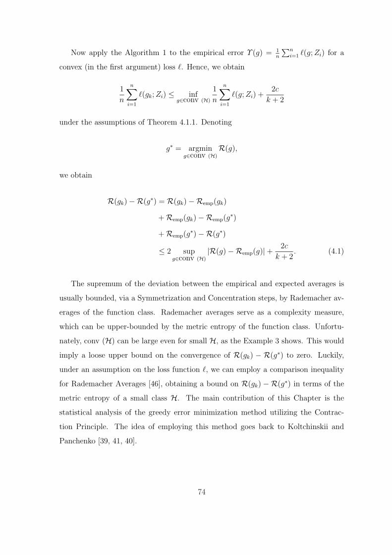
Now apply the Algorithm 1 to the empirical error Υ (g) = 1n
∑ni=1 `(g; Zi) for a
convex (in the first argument) loss `. Hence, we obtain
1
n
n∑i=1
`(gk; Zi) ≤ infg∈conv (H)
1
n
n∑i=1
`(g; Zi) +2c
k + 2
under the assumptions of Theorem 4.1.1. Denoting
g∗ = argming∈conv (H)
R(g),
we obtain
R(gk)−R(g∗) = R(gk)−Remp(gk)
+Remp(gk)−Remp(g∗)
+Remp(g∗)−R(g∗)
≤ 2 supg∈conv (H)
|R(g)−Remp(g)|+ 2c
k + 2. (4.1)
The supremum of the deviation between the empirical and expected averages is
usually bounded, via a Symmetrization and Concentration steps, by Rademacher av-
erages of the function class. Rademacher averages serve as a complexity measure,
which can be upper-bounded by the metric entropy of the function class. Unfortu-
nately, conv (H) can be large even for small H, as the Example 3 shows. This would
imply a loose upper bound on the convergence of R(gk) − R(g∗) to zero. Luckily,
under an assumption on the loss function `, we can employ a comparison inequality
for Rademacher Averages [46], obtaining a bound on R(gk) −R(g∗) in terms of the
metric entropy of a small class H. The main contribution of this Chapter is the
statistical analysis of the greedy error minimization method utilizing the Contrac-
tion Principle. The idea of employing this method goes back to Koltchinskii and
Panchenko [39, 41, 40].
74

a
-1 -1
b1
100
1 1
Figure 4-1: Step-up and step-down functions on the [0, 1] interval
Example 3. Let H be the class of simple step-up and step-down functions on the [0, 1]
interval, parametrized by a and b, as shown in Figure 4-1. The Vapnik-Chervonenkis
dimension of H is two. Let F = conv H. First, rescale the functions:
f =T∑
i=1
λihi = 2T∑
i=1
λi
(hi + 1
2
)− 1 = 2f ′ − 1
where
f ′ =T∑
i=1
λih′i
and
h′i =hi + 1
2.
We can generate any non-decreasing function f ′ such that f ′(0) = 0 and f ′(1) = 1.
Similarly, we can generate any non-increasing f ′ such that f ′(0) = 1 and f ′(1) = 0.
Rescaling back to f , we can get any non-increasing and non-decreasing functions of
the form
-1 -1
1100
1 1
2f1f
75
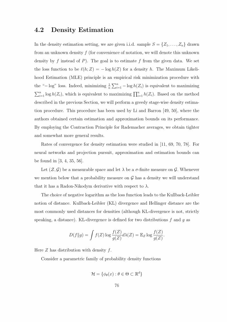
4.2 Density Estimation
In the density estimation setting, we are given i.i.d. sample S = Z1, . . . , Zn drawn
from an unknown density f (for convenience of notation, we will denote this unknown
density by f instead of P ). The goal is to estimate f from the given data. We set
the loss function to be `(h; Z) = − log h(Z) for a density h. The Maximum Likeli-
hood Estimation (MLE) principle is an empirical risk minimization procedure with
the “− log” loss. Indeed, minimizing 1n
∑ni=1− log h(Zi) is equivalent to maximizing
∑ni=1 log h(Zi), which is equivalent to maximizing
∏ni=1 h(Zi). Based on the method
described in the previous Section, we will perform a greedy stage-wise density estima-
tion procedure. This procedure has been used by Li and Barron [49, 50], where the
authors obtained certain estimation and approximation bounds on its performance.
By employing the Contraction Principle for Rademacher averages, we obtain tighter
and somewhat more general results.
Rates of convergence for density estimation were studied in [11, 69, 70, 78]. For
neural networks and projection pursuit, approximation and estimation bounds can
be found in [3, 4, 35, 56].
Let (Z,G) be a measurable space and let λ be a σ-finite measure on G. Whenever
we mention below that a probability measure on G has a density we will understand
that it has a Radon-Nikodym derivative with respect to λ.
The choice of negative logarithm as the loss function leads to the Kullback-Leibler
notion of distance. Kullback-Leibler (KL) divergence and Hellinger distance are the
most commonly used distances for densities (although KL-divergence is not, strictly
speaking, a distance). KL-divergence is defined for two distributions f and g as
D(f‖g) =
∫f(Z) log
f(Z)
g(Z)dλ(Z) = EZ log
f(Z)
g(Z).
Here Z has distribution with density f .
Consider a parametric family of probability density functions
H = φθ(x) : θ ∈ Θ ⊂ Rd
76
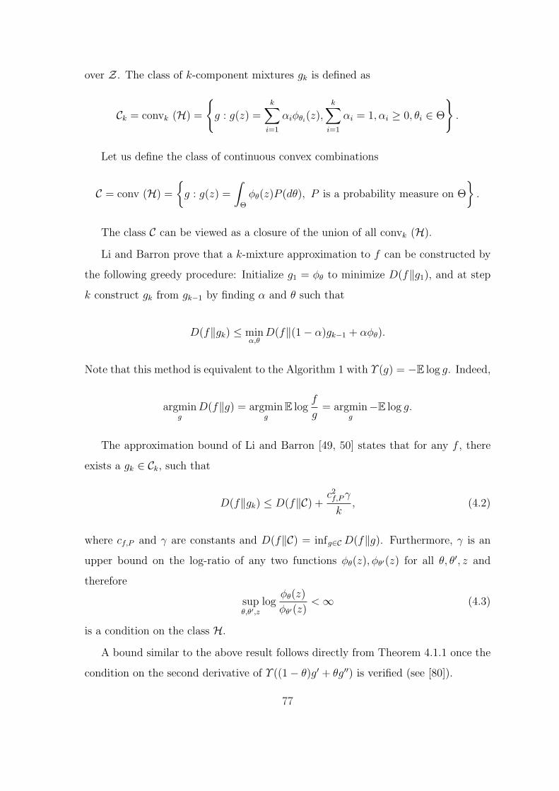
over Z. The class of k-component mixtures gk is defined as
Ck = convk (H) =
g : g(z) =
k∑i=1
αiφθi(z),
k∑i=1
αi = 1, αi ≥ 0, θi ∈ Θ
.
Let us define the class of continuous convex combinations
C = conv (H) =
g : g(z) =
∫
Θ
φθ(z)P (dθ), P is a probability measure on Θ
.
The class C can be viewed as a closure of the union of all convk (H).
Li and Barron prove that a k-mixture approximation to f can be constructed by
the following greedy procedure: Initialize g1 = φθ to minimize D(f‖g1), and at step
k construct gk from gk−1 by finding α and θ such that
D(f‖gk) ≤ minα,θ
D(f‖(1− α)gk−1 + αφθ).
Note that this method is equivalent to the Algorithm 1 with Υ (g) = −E log g. Indeed,
argming
D(f‖g) = argming
E logf
g= argmin
g−E log g.
The approximation bound of Li and Barron [49, 50] states that for any f , there
exists a gk ∈ Ck, such that
D(f‖gk) ≤ D(f‖C) +c2f,P γ
k, (4.2)
where cf,P and γ are constants and D(f‖C) = infg∈C D(f‖g). Furthermore, γ is an
upper bound on the log-ratio of any two functions φθ(z), φθ′(z) for all θ, θ′, z and
therefore
supθ,θ′,z
logφθ(z)
φθ′(z)< ∞ (4.3)
is a condition on the class H.
A bound similar to the above result follows directly from Theorem 4.1.1 once the
condition on the second derivative of Υ ((1− θ)g′ + θg′′) is verified (see [80]).
77

Of course, greedy minimization of −E log g is not possible since f is unknown. As
motivated in Chapter 2, we aim to minimize the empirical counterpart. A connection
between KL-divergence and Maximum Likelihood suggests the following method to
compute the estimate gk from the data by greedily choosing φθ at step k so that
n∑i=1
log gk(Zi) ≥ maxα,θ
n∑i=1
log[(1− α)gk−1(Zi) + αφθ(Zi)]. (4.4)
This procedure corresponds to Algorithm 1 with Υ (g) = −∑ni=1 log g(Zi).
Li and Barron proved the following theorem:
Theorem 4.2.1. Let gk(x) be either the maximizer of the likelihood over k-component
mixtures or, more generally, any sequence of density estimates satisfying (4.4). As-
sume additionally that Θ is a d-dimensional cube with side-length A, and that
supz∈Z
| log φθ(z)− log φθ′(z)| ≤ B
d∑j
|θj − θ′j| (4.5)
for any θ, θ′ ∈ Θ. Then
E [D(f‖gk)]−D(f‖C) ≤ c1
k+
c2k
nlog(nc3), (4.6)
where c1, c2, c3 are constants (dependent on A,B, d).
The above bound combines the approximation and estimation results. Note that
the first term decreases with the number of components k, while the second term
increases. The rate of convergence for the optimal k is therefore O(√
log nn
).
4.2.1 Main Results
We assume that the densities in H are bounded above and below by some constants a
and b, respectively. This boundedness naturally extends to the convex combinations
as well. We prove the following results:
Theorem 4.2.2. Suppose a ≤ φθ ≤ b for all φθ ∈ H. For gk(z) being either the
78

maximizer of the likelihood over k-component mixtures or more generally any sequence
of density estimates satisfying (4.4),
E [D(f‖gk)]−D(f‖C) ≤ c1
k+ E
[c2√n
∫ b
0
log1/2D(H, ε, dn)dε
],
where c1, c2 are constants (dependent on a, b) and D(H, ε, dn) is the ε-covering number
of H with respect to empirical distance dn (d2n(φ1, φ2) = 1
n
∑ni=1(φ1(Zi)− φ2(Zi))
2).
Corollary 4.2.1. Under the conditions of Theorem 4.2.1 (i.e. H satisfying condi-
tion (4.5) and Θ being a cube with side-length A) and assuming boundedness of the
densities, the bound of Theorem 4.2.2 becomes
E [D(f‖gk)]−D(f‖C) ≤ c1
k+
c2√n
,
where c1 and c2 are constants (dependent on a, b, A, B, d).
Corollary 4.2.2. The bound of Corollary 4.2.1 holds for the class of (truncated)
Gaussian densities H = fµ,σ : gµ,σ(z) = 1Zµ,σ
1σ√
2πexp
(− (z−µ)2
2σ2
), |µ| ≤ M, σmin ≤
σ ≤ σmax over a compact domain Z ( Zµ,σ is needed for normalization).
Remark 4.2.1. Theorem 4.2.2 hides the dependence of constants c1, c2 on a and b for
the sake of easy comparison to Theorem 4.2.1. We now state the result with explicit
dependence on a and b:
D(f‖gk)−D(f‖C) ≤ 1√n
(1
aE
[c1
∫ b
0
log1/2D(H, ε, dn)dε
]+
8
a
)
+
√t
n
(2√
2 logb
a
)+
1
k
8b2
a2
(2 + log
b
a
)
with probability at least 1− e−t, or, by integrating,
79

E [D(f‖gk)]−D(f‖C) ≤ 1√n
(1
aE
[c1
∫ b
0
log1/2D(H, ε, dn)dε
]+
8
a+ 2
√2 log
b
a
)
+1
k
8b2
a2
(2 + log
b
a
),
where c1 is an absolute constant.
Remark 4.2.2. Upper and lower bounds a and b are determined by the class H.
Assume there exists a sequence of truncations fi of f , such that ai ≤ fi(z) ≤ bi
for all z ∈ Z, and ai is decreasing and bi increasing. Further assume that each
class Hi contains functions bounded by ai and bi. As the number of samples n grows,
one can choose more and more complex models Hi. If ai is a decreasing function of
n and bi is an increasing function of n, Remark 4.2.1 provides the rate for learning
fi, the truncated version of f . This could be applied, for instance, to a sequence of
classes Hi of Gaussian densities over an increasing domain and an increasing range
of variances.
4.2.2 Discussion of the Results
The result of Theorem 4.2.2 is two-fold. The first implication concerns dependence of
the bound on k, the number of components. Our results show that there is an esti-
mation bound of the order O( 1√n) that does not depend on k. Therefore, the number
of components is not a trade-off that has to be made with the approximation part
(which decreases with k). The bound also suggests that the number of components
k should be chosen to be O(√
n).
The second implication concerns the rate of convergence in terms of n, the number
of samples. The rate of convergence (in the sense of KL-divergence) of the estimated
mixture to the true density is of the order O(1/√
n). As Corollary 4.2.1 shows, for the
specific class H considered by Li and Barron, the Dudley integral converges and does
not depend on n. We therefore improve the results of Li and Barron by removing the
log n factor. Furthermore, the result of this paper holds for general base classes H
80
with a converging entropy integral, extending the result of Li and Barron. Note that
the bound of Theorem 4.2.2 is in terms of the metric entropy of H, as opposed to the
metric entropy of C. This is a strong result because the convex class C can be very
large even for small H (see Example 3).
Rates of convergence for the MLE in mixture models were studied by Sara van
de Geer [69]. As the author notes, the optimality of the rates depends primarily on
the optimality of the entropy calculations. Unfortunately, in the results of [69], the
entropy of the convex class appears in the bounds, which is undesirable. Moreover,
only finite combinations are considered.
Wong and Shen [78] also considered density estimation, deriving rates of conver-
gence in Hellinger distance for a class of bounded Lipschitz densities. In their work,
a bound on the metric entropy of the whole class appears.
An advantage of the approach of [69] is the use of Hellinger distance to avoid
problems near zero. Li and Barron address this problem by requiring (4.3), which
is boundedness of the log of the ratio of two densities. Birge and Massart ([11],
page 122) cite a counterexample of Bahadur (1958) which shows that even with a
compact parameter space, M.L.E. can diverge when likelihood ratios are unbounded.
Unfortunately, boundedness of the ratios of densities is not enough for the proofs of
this paper. We assume boundedness of the densities themselves. This is critical in
one step of the proof, when the contraction principle is used (for the second time).
Although the boundedness condition seems a somewhat strict requirement, note that
a class of densities that satisfies (4.3), but not boundedness of the densities, has to
contain functions which all go to zero (or infinity) in exactly the same manner. Also
note that on a non-compact domain IR even a simple class of Gaussian densities does
not satisfy (4.3). Indeed, the log-ratio of the tails of two Gaussians with the same
variance but different means becomes infinite. If one considers a compact domain X ,
the boundedness of densities assumption does not seem very restrictive.
The proof technique of this paper seems to be a powerful general method for
bounding uniform deviations of empirical and expected quantities. The main ingre-
dients of the proof are the Comparison inequality for Rademacher processes and the
81
fact that Rademacher averages (as defined in Lemma 2.5.1) of the convex hull are
equivalent to those of the base class.
4.2.3 Proofs
Assume
0 < a ≤ φθ(z) ≤ b ∀z ∈ Z, ∀φθ ∈ H.
Constants which depend only on a and b will be denoted by c with various subscripts.
The values of the constants might change from line to line.
Theorem 4.2.3. For any fixed density f and S = (Z1, . . . , Zn) drawn i.i.d from f ,
with probability at least 1− e−t,
supg∈C
∣∣∣∣∣1
n
n∑i=1
log g(Zi)− E log g
∣∣∣∣∣ ≤ E[
c1√n
∫ b
0
log1/2D(H, ε, dn)dε
]+ c2
√t
n,
where c1 and c2 are constants that depend on a and b.
Proof. First, we apply Lemma 2.4.3 to the random variable
Tn(Z1, . . . , Zn) = supg∈C
∣∣∣∣∣1
n
n∑i=1
log g(Zi)− E log g
∣∣∣∣∣ .
Let ti = log g(zi) and t′i = log g(z′i). The bound on the martingale difference follows:
|Tn(z1, . . . , z′i, . . . , zn)− Z(Z1, . . . , Zn)|
=
∣∣∣∣supg∈C
∣∣∣∣E log g − 1
n(t1 + . . . + ti + . . . + tn)
∣∣∣∣
− supg∈C
∣∣∣∣E log g − 1
n(t1 + . . . + t′i + . . . + tn)
∣∣∣∣∣∣∣∣
≤ supg∈C
1
n|log g(z′i)− log g(zi)| ≤ 1
nlog
b
a= ci.
The above chain of inequalities holds because of the triangle inequality and the prop-
82

erties of sup. Applying McDiarmid’s inequality (see Lemma 2.4.3),
P (Tn − ETn > u) ≤ exp
(− u2
2∑
c2i
)= exp
(− nu2
2(log b
a
)2
).
Therefore,
supg∈C
∣∣∣∣∣1
n
n∑i=1
log g(Zi)− E log g
∣∣∣∣∣ ≤ E supg∈C
∣∣∣∣∣1
n
n∑i=1
log g(Zi)− E log g
∣∣∣∣∣ +√
2 logb
a
√t
n
with probability at least 1− e−t and by Lemma 2.5.1,
E supg∈C
∣∣∣∣∣1
n
n∑i=1
log g(Zi)− E log g
∣∣∣∣∣ ≤ 2E supg∈C
∣∣∣∣∣1
n
n∑i=1
εi log g(Zi)
∣∣∣∣∣ .
Combining,
supg∈C
∣∣∣∣∣1
n
n∑i=1
log g(Zi)− E log g
∣∣∣∣∣ ≤ 2E supg∈C
∣∣∣∣∣1
n
n∑i=1
εi log g(Zi)
∣∣∣∣∣ +√
2 logb
a
√t
n
with probability at least 1− e−t.
Therefore, instead of bounding the difference between the “empirical” and the “ex-
pectation”, it is enough to bound the above expectation of the Rademacher average.
This is a simpler task, but first we have to deal with the logarithm in the Rademacher
sum. To eliminate this difficulty, we apply Lemma 2.5.2. Once we reduce our problem
to bounding the Rademacher sum of the basis functions supφ∈H∣∣ 1n
∑ni=1 εiφ(Zi)
∣∣, we
will be able to use the entropy of class H.
Let pi = g(xi)− 1 and note that a− 1 ≤ pi ≤ b− 1. Consider φ(p) = log(1 + p).
The largest derivative of log(1 + p) on the interval p ∈ [a − 1, b − 1] is at p = a − 1
and is equal to 1/a. So, a log(p + 1) is 1-Lipschitz. Also, φ(0) = 0. By Lemma 2.5.2
83
applied to φ(p),
2E supg∈C
∣∣∣∣∣1
n
n∑i=1
εi log g(Zi)
∣∣∣∣∣ = 2E supg∈C
∣∣∣∣∣1
n
n∑1
εiφ(pi)
∣∣∣∣∣
≤ 41
aE sup
g∈C
∣∣∣∣∣1
n
n∑i=1
εig(Zi)− 1
n
n∑1
εi
∣∣∣∣∣
≤ 41
aE sup
g∈C
∣∣∣∣∣1
n
n∑i=1
εig(Zi)
∣∣∣∣∣ + 41
aEε
∣∣∣∣∣1
n
n∑i=1
εi
∣∣∣∣∣
≤ 41
aE sup
g∈C
∣∣∣∣∣1
n
n∑i=1
εig(Zi)
∣∣∣∣∣ +4
a
1√n
.
The last inequality holds because
Eε
∣∣∣∣∣1
n
n∑i=1
εi
∣∣∣∣∣ ≤Eε
(1
n
n∑i=1
εi
)2
1/2
=1√n
.
Combining the inequalities, with probability at least 1− e−t
supg∈C
∣∣∣∣∣1
n
n∑i=1
log g(Zi)− E log g
∣∣∣∣∣ ≤ 4
aE sup
g∈C
∣∣∣∣∣1
n
n∑i=1
εig(Zi)
∣∣∣∣∣ +√
2 logb
a
√t
n+
4
a
1√n
.
The power of using Rademacher averages to estimate complexity comes from the
fact that the Rademacher averages of a class are equal to those of the convex hull.
Indeed, consider
supg∈C
∣∣∣∣∣1
n
n∑i=1
εig(Zi)
∣∣∣∣∣
with g(z) =∫
θφθ(z)P (dθ). Since a linear functional over convex combinations
achieves its maximum value at the vertices, the above supremum is equal to
supθ
∣∣∣∣∣1
n
n∑i=1
εiφθ(Zi)
∣∣∣∣∣ ,
84

the corresponding supremum on the basis functions φ ∈ H. Therefore,
Eε supg∈C
∣∣∣∣∣1
n
n∑i=1
εig(Zi)
∣∣∣∣∣ = Eε supθ∈Θ
∣∣∣∣∣1
n
n∑i=1
εiφθ(Zi)
∣∣∣∣∣ .
Next, we use the following classical result (see [71]),
Eε supφ∈H
∣∣∣∣∣1
n
n∑i=1
εiφ(Zi)
∣∣∣∣∣ ≤c1√n
∫ b
0
log1/2D(H, ε, dn)dε,
where dn is the empirical distance with respect to the set Z1, . . . , Zn.
Combining the results, the following holds with probability at least 1− e−t:
supg∈C
∣∣∣∣∣1
n
n∑i=1
log g(Zi)− E log g
∣∣∣∣∣ ≤[
c1√n
∫ b
0
log1/2D(H, ε, dn)dε
]+ c2
√t
n.
Remark 4.2.3. If H is a VC-subgraph with VC dimension V , the Dudley integral
above is bounded by c√
V and we obtain O(1/√
n) convergence. One example of such
a class is the class of (truncated) Gaussian densities over a compact domain and with
bounded variance (see Corollary 4.2.2). Another example is the class considered in
[49], and its cover is computed in the proof of Corollary 4.2.1. More information on
the classes with converging Dudley integral and examples of VC-subgraph classes can
be found in [25, 71].
We are now ready to prove Theorem 4.2.2:
85

Proof.
D(f‖gk)−D(f‖gk) = E log gk − E log gk
=
(E log gk − 1
n
n∑i=1
log gk(Zi)
)
+
(1
n
n∑i=1
log gk(Zi)− 1
n
n∑i=1
log gk(Zi)
)
+
(1
n
n∑i=1
log gk(Zi)− E log gk
)
≤ 2 supg∈C
∣∣∣∣∣1
n
n∑i=1
log g(Zi)− E log g
∣∣∣∣∣
+
(1
n
n∑i=1
log gk(Zi)− 1
n
n∑i=1
log gk(Zi)
)
≤ E[
c1√n
∫ b
0
log1/2D(H, ε, dn)dε
]+ c2
√t
n+
1
n
n∑i=1
loggk(Zi)
gk(Zi)
with probability at least 1− e−t (by Theorem 4.2.3). Note that 1n
∑ni=1 log gk(Zi)
gk(Zi)≤ 0
if fk is constructed by maximizing the likelihood over k-component mixtures. If it
is constructed by the Algorithm 1, Theorem 4.1.1 shows that gk achieves “almost
maximum likelihood”. Another proof of this result is given on page 27 of [50], or
section 3 of [49]:
∀g ∈ C, 1
n
n∑i=1
log(gk(Zi))(ni) ≥ 1
n
n∑i=1
log(g(Zi))(ni)− γc2Fn,P
k.
Here c2Fn,P = (1/n)
∑ni=1
Rφ2
θ(zi)P (dθ)
(R
φθ(zi)P (dθ))2 ≤ b2
a2 and γ = 4 log(3√
e) + 4 log ba. Hence,
with probability at least 1− e−t,
D(f‖gk)−D(f‖gk) ≤ E[
c1√n
∫ b
0
log1/2D(H, ε, dn)dε
]+ c2
√t
n+
c3
k.
We now write the overall error of estimating an unknown density f as the sum
of approximation and estimation errors. The former is bounded by (4.2) and the
latter is bounded as above. Note again that c2f,P and γ in the approximation bound
86
(4.2) are bounded above by constants which depend only on a and b. Therefore, with
probability at least 1− e−t,
D(f‖gk)−D(f‖C) = (D(f‖gk)−D(f‖C)) + (D(f‖gk)−D(f‖gk))
≤ c
k+
[c1√n
∫ b
0
log1/2D(H, ε, dn)dε
]+ c2
√t
n. (4.7)
Remark 4.2.4. Note that we could have obtained the above bound from the Equation
4.1 without the decomposition into the approximation and estimation errors.
Finally, we rewrite the above probabilistic statement as a statement in terms of
expectations. Let ζ = ck
+ E[
c1√n
∫ b
0log1/2D(H, ε, dn)dε
]and ξ = D(f‖gk)−D(f‖C).
We have shown that P(ξ ≥ ζ + c2
√tn
)≤ e−t. Since ξ ≥ 0,
E [ξ] =
∫ ζ
0
P (ξ > u) du +
∫ ∞
ζ
P (ξ > u) du ≤ ζ +
∫ ∞
0
P (ξ > u + ζ) du.
Now set u = c2
√tn. Then t = c3nu2 and E [ξ] ≤ ζ +
∫∞0
e−c3nu2du ≤ ζ + c√
n.
Hence,
E [D(f‖gk)]−D(f‖C) ≤ c1
k+ E
[c2√n
∫ b
0
log1/2D(H, ε, dn)dε
].
Remark 4.2.5. Inequality (4.7) is much stronger than the result of Theorem 4.2.2
because it reveals the tail behavior of D(f‖gk) −D(f‖C). Nevertheless, to be able to
compare our results to those of Li and Barron, we present our results in terms of
expectations.
Remark 4.2.6. In the actual proof of the bounds, Li and Barron [50, 49] use a
specific sequence of αi for the finite combinations. The authors take α1 = 1, α2 = 12,
87

and αk = 2k
for k ≥ 2. It can be shown that in this case
gk =2
k(k − 1)
(1
2φ1 +
1
2φ2 +
k∑m=3
(m− 1)φm
),
so the later choices have more weight.
We now prove Corollary 4.2.1:
Proof. Since we consider bounded densities a ≤ φθ ≤ b, condition (4.5) implies that
∀z, log
(φθ(z)− φθ′(z)
b+ 1
)≤ B|θ − θ′|L1 .
This allows us to bound L∞ distances between functions in H in terms of the L1
distances between the corresponding parameters. Since Θ is a d-dimensional cube of
side-length A, we can cover Θ by(
Aδ
)dballs of L1-radius d δ
2. This cover induces a
cover of H. For any φθ there exists an element of the cover φθ′ , so that
dn(φθ, φθ′) ≤ |φθ − φθ′|∞ ≤ beB dδ2 − b = ε.
Therefore, δ =2 log( ε
b+1)
Bdand the cardinality of the cover is (A
δ)d =
(ABd
2 log( εb+1)
)d
.
Hence, ∫ b
0
log1/2D(H, ε, dn)dε =
∫ b
0
√d log
ABd
2 log(
εb+ 1
)dε.
A straightforward calculation shows that the integral above converges.
By creating a simple net over the class H in Corollary 4.2.2, one can easily show
that H has a finite cover D(H, ε, dn) = Kε2
, for some constant K. Corollary 4.2.2
follows.
4.3 Classification
The analysis of the greedy algorithm (Algorithm 1) in the classification setting fol-
lows along the same lines as that of density estimation. Once the loss function in
88

Equation 4.1 is specified, the Concentration and Symmetrization steps can be per-
formed similarly to the proofs of the previous Section. Similar proofs have been done
independently by Mannor et al [53].
Suppose Z = X × Y and Y = −1, 1. Let `(g; Z) = `(yg(x)) such that
`(yg(x)) ≥ I(yg(x) ≤ 0)
and `(·) is a convex function with a Lipschitz constant L. For natural convex loss
functions, the Lipschitz constant is finite if the functions g are bounded.
0
1
`(yg(x))
I(yg(x) ≤ 0)
yg(x)
Figure 4-2: Convex loss ` upper-bounds the indicator loss.
By performing the greedy minimization procedure with Υ (g) = 1n
∑ni=1 `(Yig(Xi))
over the convex hull conv (H), we obtain gk such that, according to the Equation 4.1,
R(gk)−R(g∗) ≤ 2 supg∈conv (H)
|R(g)−Remp(g)|+ 2c
k + 2.
Zhang [80] provides the specific constants c for common loss functions `.
Using the Symmetrization and Concentration steps as well as employing the com-
parison inequality for Rademacher processes, we obtain a result similar to Theorem
4.2.3:
89
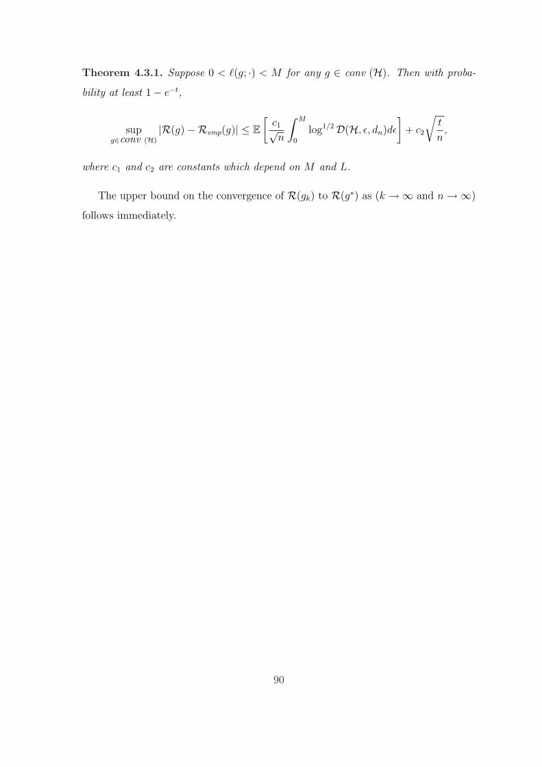
Theorem 4.3.1. Suppose 0 < `(g; ·) < M for any g ∈ conv (H). Then with proba-
bility at least 1− e−t,
supg∈conv (H)
|R(g)−Remp(g)| ≤ E[
c1√n
∫ M
0
log1/2D(H, ε, dn)dε
]+ c2
√t
n,
where c1 and c2 are constants which depend on M and L.
The upper bound on the convergence of R(gk) to R(g∗) as (k →∞ and n →∞)
follows immediately.
90

Chapter 5
Stability of Empirical Risk
Minimization over Donsker Classes
The results of this Chapter appear partially in [18, 19].
5.1 Introduction
Empirical risk minimization (ERM) algorithm has been studied in learning theory to
a great extent. Vapnik and Chervonenkis [74, 76] showed necessary and sufficient con-
ditions for its consistency. In recent developments, [6, 8, 7, 38] proved sharp bounds
on the performance of ERM. Tools from empirical process theory have been success-
fully applied, and, in particular, it has been shown that the localized Rademacher
averages play an important role in studying the behavior of the ERM algorithm.
In this Chapter we are not directly concerned with rates of performance of ERM.
Rather, we prove some properties of ERM algorithms, which, to our knowledge, do
not appear in the literature. The analysis of this Chapter has been motivated by
the study of algorithmic stability: the behavior of a learning algorithm with respect
to perturbations of the training set. Algorithmic stability has been studied in the
recent years as an alternative to the classical (complexity-oriented) approach to de-
riving generalization bounds [16, 45, 55, 58, 60]. Motivation for studying algorithmic
stability comes, in part, from the work of [22]. Their results indicate that for any al-
91
gorithm, the performance of the leave-one-out estimator of expected error is bounded
by L1-stability of the algorithm, i.e. by the average L1 distance between hypotheses
on similar samples. This result can be used to derive bounds on the performance of
the leave-one-out estimate for algorithms such as k-Nearest Neighbors. It is impor-
tant to note that no class of finite complexity is searched by algorithms like k-NN,
and so the classical approach of using complexity of the hypothesis space fails.
Further important results were proved by Bousquet and Elisseeff [16], where a
large family of algorithms (Tikhonov regularization based methods) has been shown to
possess a strong L∞ stability with respect to changes of single samples of the training
set, and exponential bounds have been proved for the generalization error in terms
of empirical error. Tikhonov regularization based algorithms minimize the empirical
error plus a stabilizer, and are closely related to ERM. Though ERM is not, in general,
L∞-stable, it is L1-stable over certain classes of functions, as one of the results below
shows. To the best of our knowledge, the outcomes of the present Chapter do not
follow directly from results available in the machine learning literature. In fact we
had to turn to the empirical process theory (see Section 2.5) for the mathematical
tools necessary for studying stability of ERM.
Various assumptions on the function class, over which ERM is performed, have
been considered recently to obtain fast rates on the performance of ERM. The im-
portance of having a unique best function in the class has been shown by [48]: the
difficult learning problems seem to be the ones where two minimizers of the expected
error exist and are far apart. Although we do not address the question of performance
rates here, our results does shed some light on the behavior of ERM when two (or
more) minimizers of expected error exist. Our results imply that, under a certain
weak condition on the class, as the expected performance of empirical minimizers ap-
proaches the best in the class, a jump to a different part of the function class becomes
less and less likely.
Some algorithmic implications of our results are straight-forward. For example, in
the context of on-line learning, when a point is added to the training set, with high
probability one has to search for empirical minimizers in a small L1-ball around the
92

current hypothesis, which can be a tractable problem. Moreover, it seems plausible
that L1-stability can have consequences for computational complexity of ERM. While
it has been shown that ERM is NP-hard even for simple function classes (see e.g. [9]),
our results could allow more optimistic average-case analysis.
Since ERM minimizes empirical error instead of expected error, it is reasonable to
require that the two quantities become close uniformly over the class, as the number
of examples grows. Hence, ERM is a sound strategy only if the function class is
uniform Glivenko-Cantelli, that is, it satisfies the uniform law of large numbers. In
this Chapter we focus our attention on more restricted family of function classes:
Donsker classes (see Section 2.5). These are classes satisfying not only the law of
large numbers, but also a version of the central limit theorem. Though a more
restricted family of classes, Donsker classes are still quite general. In particular,
uniform Donsker and uniform Glivenko-Cantelli properties are equivalent in the case
of binary-valued functions (and also equivalent to finiteness of VC dimension). The
central limit theorem for Donsker classes states a form of convergence of the empirical
process to a Gaussian process with a specific covariance structure (e.g. [25, 71]).
This structure is used in the proof of the main result of this Chapter to control the
correlation of the empirical errors of ERM minimizers on similar samples.
This Chapter is organized as follows. In Section 5.2 we introduce the notation
and background results. Section 5.3 presents the main result, which is proved in
the appendix using tools from empirical process theory. In Section 5.4, we show L1-
stability of ERM over Donsker classes as an application of the main result of Section
5.3. In Section 5.5 we show an improvement (in terms of the rates) of the main result
under a suitable Komlos-Major-Tusnady condition and an assumption on entropy
growth. Section 5.6 combines the results of Sections 5.4 and 5.5 and uses a uniform
ratio limit theorem to obtain fast rates of decay on the deviations of expected errors
of almost-ERM solutions, thus establishing strong expected error stability of ERM (see
Chapter 3). Several further applications of the results are considered in Section 5.7.
Most of the proofs are postponed to the Appendix. Section 5.8 is a final summary of
the results.
93

5.2 Notation
Let (Z,G) be a measurable space. Let P be a probability measure on (Z,G) and
Z1, . . . , Zn be independent copies of Z with distribution P . Let F be a class of
functions from Z to R. In the setting of learning theory, samples Z are input-output
pairs (X, Y ) and for f ∈ F , f(Z) measures how well the relationship between X
and Y is captured by f . Hence, F is usually the loss class of some other function
class H, i.e. F = L(H) (see Section 2.1). The goal is to minimize Pf = Ef(Z)
where information about the unknown P is given only through the finite sample
S = (Z1, . . . , Zn). Define the empirical measure as Pn = 1n
∑ni=1 δZi
.
Definition 5.2.1. Given a sample S,
fS := argminf∈F
Pnf = argminf∈F
1
n
n∑i=1
f(Zi)
is a minimizer of the empirical risk (empirical error), if the minimum exists.
Since an exact minimizer of the empirical risk might not exist, as well as for
algorithmic reasons, we consider the set of almost-minimizers of empirical risk.
Definition 5.2.2. Given ξ ≥ 0 and S, define the set of almost empirical minimizers
MξS = f ∈ F : Pnf − inf
g∈FPng ≤ ξ
and define its diameter as
diamMξS = sup
f,g∈MξS
‖f − g‖ .
Note that MξS ⊂ Mξ′
S whenever ξ ≤ ξ′. Moreover, if f, g ∈ MξS and h =
(1− λ)f + λg ∈ F , then h ∈ MξS by linearity of the average. Hence, if F is convex,
so is MξS for any ξ > 0.
The ‖·‖ in the above definition is the seminorm on F induced by symmetric
94

bilinear product
〈f, f ′〉 = P (f − Pf) (f ′ − Pf ′) .
This is a natural measure of distance between functions, as will become apparent
later, because of the central role of the covariance structure of Brownian bridges in
our proofs. The results obtained for the seminorm ‖·‖ will be easily extended to the
L2(P ) norm, thanks to the close relation of these two notions of distance.
5.3 Main Result
We now state the main result of this Chapter.
Theorem 5.3.1. Let F be a P-Donsker class. For any sequence ξ(n) = o(n−1/2),
diamMξ(n)S
P ∗−→ 0.
The outer probability P ∗ above is due to measurability issues. Definitions and
results on various types of convergence, as well as ways to deal with measurability
issues arising in the proofs, are based on the rigorous book of [71].
Before turning to the proof of Theorem 5.3.1, let us discuss the geometry of the
function class F and its relation to the results. Recall that P -Donsker class F is also
a P -Glivenko-Cantelli class, and so empirical risk minimization on F is consistent:
as n →∞,
PfSP ∗−→ inf
g∈FPg.
For simplicity, assume for a second that functions f ∈ F are the square loss functions
over some class H and Z = X × Y :
F = f(z) = `(h, z) = (h(x)− y)2 : h ∈ H = L(H).
Figures 5-1 through 5-4 depict four important possibilities regarding the geometry of
the function class.
95

H
h∗
Figure 5-1: Realizable setting.
H
h∗
Figure 5-2: Single minimum of ex-pected error.
H
h2
h1
h∗
Figure 5-3: Finite number of minimiz-ers of expected error.
H
h∗
Figure 5-4: Infinitely many minimizersof expected error.
The simplest situation, that of realizable setting, occurs when the target function
h∗ (the function achieving the zero expected error) belongs to the class H. In this
case, one can show that the empirical minimizers converge to this function in L2(P )
distance and, by the triangle inequality, the distance between two empirical minimiz-
ers over different sets converges to zero in probability. In fact, one can upper-bound
the rate of this decrease. Similar behavior can be shown for non-realizable settings
when there is a single (Figure 5-2) best function in the given class. For a finite number
(Figure 5-3) of best functions in the given class, one can show, based on the binomial
result, that Ω(√
n) changes is enough to induce a large jump of the empirical mini-
mizer. Nevertheless, in this case empirical minimization is still stable with respect to
o(√
n) changes. Hence, n−1/2 is the rate defining the transition between stability and
instability in the case of the finite number of minimizers of the expected error. Once
96
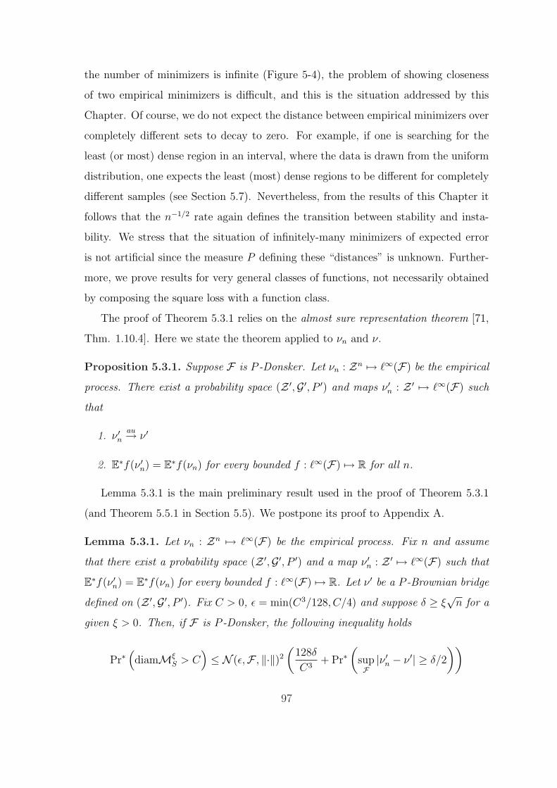
the number of minimizers is infinite (Figure 5-4), the problem of showing closeness
of two empirical minimizers is difficult, and this is the situation addressed by this
Chapter. Of course, we do not expect the distance between empirical minimizers over
completely different sets to decay to zero. For example, if one is searching for the
least (or most) dense region in an interval, where the data is drawn from the uniform
distribution, one expects the least (most) dense regions to be different for completely
different samples (see Section 5.7). Nevertheless, from the results of this Chapter it
follows that the n−1/2 rate again defines the transition between stability and insta-
bility. We stress that the situation of infinitely-many minimizers of expected error
is not artificial since the measure P defining these “distances” is unknown. Further-
more, we prove results for very general classes of functions, not necessarily obtained
by composing the square loss with a function class.
The proof of Theorem 5.3.1 relies on the almost sure representation theorem [71,
Thm. 1.10.4]. Here we state the theorem applied to νn and ν.
Proposition 5.3.1. Suppose F is P -Donsker. Let νn : Zn 7→ `∞(F) be the empirical
process. There exist a probability space (Z ′,G ′, P ′) and maps ν ′n : Z ′ 7→ `∞(F) such
that
1. ν ′nau→ ν ′
2. E∗f(ν ′n) = E∗f(νn) for every bounded f : `∞(F) 7→ R for all n.
Lemma 5.3.1 is the main preliminary result used in the proof of Theorem 5.3.1
(and Theorem 5.5.1 in Section 5.5). We postpone its proof to Appendix A.
Lemma 5.3.1. Let νn : Zn 7→ `∞(F) be the empirical process. Fix n and assume
that there exist a probability space (Z ′,G ′, P ′) and a map ν ′n : Z ′ 7→ `∞(F) such that
E∗f(ν ′n) = E∗f(νn) for every bounded f : `∞(F) 7→ R. Let ν ′ be a P -Brownian bridge
defined on (Z ′,G ′, P ′). Fix C > 0, ε = min(C3/128, C/4) and suppose δ ≥ ξ√
n for a
given ξ > 0. Then, if F is P -Donsker, the following inequality holds
Pr∗(diamMξ
S > C)≤ N (ε,F , ‖·‖)2
(128δ
C3+ Pr∗
(supF|ν ′n − ν ′| ≥ δ/2
))
97
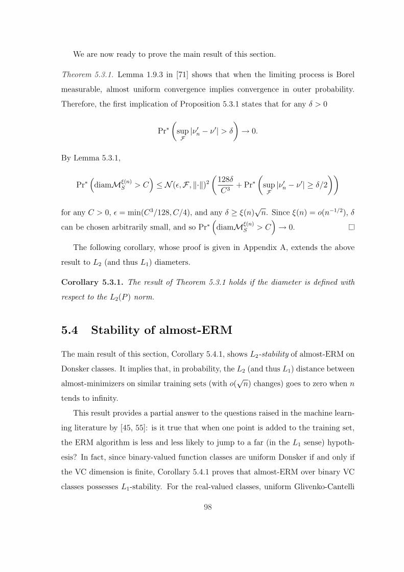
We are now ready to prove the main result of this section.
Theorem 5.3.1. Lemma 1.9.3 in [71] shows that when the limiting process is Borel
measurable, almost uniform convergence implies convergence in outer probability.
Therefore, the first implication of Proposition 5.3.1 states that for any δ > 0
Pr∗(
supF|ν ′n − ν ′| > δ
)→ 0.
By Lemma 5.3.1,
Pr∗(diamMξ(n)
S > C)≤ N (ε,F , ‖·‖)2
(128δ
C3+ Pr∗
(supF|ν ′n − ν ′| ≥ δ/2
))
for any C > 0, ε = min(C3/128, C/4), and any δ ≥ ξ(n)√
n. Since ξ(n) = o(n−1/2), δ
can be chosen arbitrarily small, and so Pr∗(diamMξ(n)
S > C)→ 0.
The following corollary, whose proof is given in Appendix A, extends the above
result to L2 (and thus L1) diameters.
Corollary 5.3.1. The result of Theorem 5.3.1 holds if the diameter is defined with
respect to the L2(P ) norm.
5.4 Stability of almost-ERM
The main result of this section, Corollary 5.4.1, shows L2-stability of almost-ERM on
Donsker classes. It implies that, in probability, the L2 (and thus L1) distance between
almost-minimizers on similar training sets (with o(√
n) changes) goes to zero when n
tends to infinity.
This result provides a partial answer to the questions raised in the machine learn-
ing literature by [45, 55]: is it true that when one point is added to the training set,
the ERM algorithm is less and less likely to jump to a far (in the L1 sense) hypoth-
esis? In fact, since binary-valued function classes are uniform Donsker if and only if
the VC dimension is finite, Corollary 5.4.1 proves that almost-ERM over binary VC
classes possesses L1-stability. For the real-valued classes, uniform Glivenko-Cantelli
98

property is weaker than uniform Donsker property, and therefore it remains unclear
if almost-ERM over uGC but not uniform Donsker classes is stable in the L1 sense.
The use of L1-stability goes back to [22], who showed that this stability is sufficient
to bound the difference between the leave-one-out error and the expected error of a
learning algorithm. In particular, Devroye and Wagner show that nearest-neighbor
rules possess L1-stability [see also 20]. Our Corollary 5.4.1 implies L1-stability of
ERM (or almost-ERM) algorithms on Donsker classes.
In the following [n] denotes the set 1, 2, . . . , n and A 4 B is the symmetric
difference of sets A and B.
Corollary 5.4.1. Assume F is P -Donsker and uniformly bounded with envelope F ≡1. For I ⊂ N, define S(I) = (Zi)i∈I . Let In ⊂ N such that Mn := |In4 [n]| = o(n1/2).
Suppose fn ∈Mξ(n)S([n]) and f ′n ∈Mξ′(n)
S(In) for some ξ(n) = o(n−1/2) and ξ′(n) = o(n−1/2).
Then
‖fn − f ′n‖ P ∗−→ 0.
The norm ‖·‖ can be replaced by L2(P ) or L1(P ) norm.
Proof. It is enough to show that f ′n ∈ Mξ′′(n)S([n]) for some ξ′′(n) = o(n−1/2) and result
follows from the Theorem 5.3.1.
1
n
∑
i∈[n]
f ′n(Zi) ≤ Mn
n+
1
n
∑i∈In
f ′n(Zi)
≤ Mn
n+|In|n
(ξ′(n) + inf
g∈F1
|In|∑i∈In
g(Zi)
)
≤ Mn
n+|In|n
ξ′(n) +1
n
∑i∈In
fn(Zi)
≤ 2Mn
n+|In|n
ξ′(n) +1
n
∑
i∈[n]
fn(Zi)
≤ 2Mn
n+|In|n
ξ′(n) + ξ(n) + infg∈F
1
n
∑
i∈[n]
g(Zi)
Define
ξ′′(n) := 2Mn
n+|In|n
ξ′(n) + ξ(n).
99
Because Mn = o(n12 ), it follows that ξ′′(n) = o(n−1/2). Corollary 5.3.1 implies con-
vergence in L2(P ), and, therefore, in L1(P ) norm.
Let us now generalize the above result to functions with a bounded Lipschitz
constant. The Lipschitz assumption allows us to study sensitivity of functions with
respect to perturbations of the data points in the space instead of complete removals
or additions.
More precisely, assume that the space Z is equipped with a distance metric d.
Furthermore, suppose Z is compact: say, Z ⊂ Bd(0, R). Suppose that F consists of
functions with a bounded Lipschitz constant L:
∀z, z′ ∈ Z, ∀f ∈ F , |f(z)− f(z′)| ≤ Ld(z, z′).
Define the “distance” between two sets S, T as follows. For sets S = z1, . . . , zn,T = z′1, . . . , z′n of equal size
d(S, T ) = infπ
1
n
|S|∑i=1
d(zi, z′π(i)).
If |S| < |T |,
d(S, T ) = infπ
1
n
|S|∑i=1
d(zi, z′π(i)) + 2R(|T | − |S|)
and if |S| > |T |,
d(S, T ) = infπ
1
n
|T |∑i=1
d(zπ(i), z′) + 2R(|S| − |T |).
In other words, the “distance” between two sets is defined as the best way to
pair up points from one set with points from the other set, and paying the constant
(diameter of the ball) for each unmatched point.
Corollary 5.4.2. Assume F is P -Donsker and uniformly bounded with envelope F ≡1. Suppose F consists of functions with a bounded Lipschitz constant L and Z ⊂Bd(0, R). Suppose fS ∈ Mξ(n)
S and fT ∈ Mξ′(n)T for some ξ(n) = o(n−1/2) and
100
ξ′(n) = o(n−1/2). If d(S, T ) = o(n−1/2), then
‖fS − fT‖ P ∗−→ 0.
The norm ‖·‖ can be replaced by L2(P ) or L1(P ) norm.
Proof. Without loss of generality suppose that n = |S| < |T |. Similarly to the proof
of Corollary 5.4.1,
1
n
∑z∈T
fS(z)− 1
n
∑z∈T
fT (z) =1
n
∑z∈T
fS(z)− 1
n
∑z∈S
fS(z)
+1
n
∑z∈S
fS(z)− 1
n
∑z∈S
fT (z)
+1
n
∑z∈S
fT (z)− 1
n
∑z∈T
fT (z)
≤ 2L
n
n∑i=1
d(zi, z′i) + 2R(|T | − |S|) + ξ(n)
In fact, since we can permute T in any suitable way, we have
1
n
∑z∈T
fS(z)− 1
n
∑z∈T
fT ≤ 2Ld(S, T ) + ξ(n).
Since both terms decaying faster than n−1/2 and fT ∈Mξ′(n)T , we have that
fS ∈Mξ′′(n)T
for ξ′′(n) = o(n−1/2). We apply Theorem 5.3.1 to obtain the result.
5.5 Rates of Decay of diamMξ(n)S
The statement of Lemma 5.3.1 reveals that the rate of the decay of the diameter
diamMξ(n)S is related to the rate at which Pr∗ (supF |ν − νn| ≥ δ) → 0 for a fixed δ.
A number of papers studied this rate of convergence, and here we refer to the notion of
101

Komlos-Major-Tusnady class (KMT class), as defined by [42]. Let ν ′n : Zn 7→ `∞(F)
be the empirical process defined on the probability space (Z ′,G ′, P ′).
Definition 5.5.1. F is called a Komlos-Major-Tusnady class with respect to P and
with the rate of convergence τn (F ∈ KMT (P ; τn)) if F is P -pregaussian and for
each n ≥ 1 there is a version ν(n) of P -Brownian bridge defined on (Z ′,G ′““““““, P ′)
such that for all t > 0,
Pr∗(
supF|ν(n) − ν ′n| ≥ τn(t + K log n)
)≤ Λe−θt
where K > 0, Λ > 0 and θ > 0 are constants, depending only on F .
Sufficient conditions for a class to be KMT (P ; n−α) have been investigated in the
literature; some results of this type can be found in [42, 62] and [25], Section 9.5(B).
The following theorem shows that for KMT classes fulfilling a suitable entropy
condition, it is possible to give explicit rates of decay for the diameter of ERM almost-
minimizers.
Theorem 5.5.1. Assume F is P -Donsker and F ∈ KMT (P ; n−α) for some α > 0.
Assume N (ε,F , ‖·‖) ≤ (Aε
)Vfor some constants A, V > 0. Let ξ(n)
√n = o(n−η),
η > 0. Then
nγdiamMξ(n)S
P ∗−→ 0
for any γ < 13(2V +1)
min(α, η).
Proof. The result of Lemma 5.3.1 is stated for a fixed n. We now choose C, ξ,
and δ depending on n as follows. Let C(n) = Bn−γ, where γ < 13(2V +1)
min(α, η)
and B > 0 is an arbitrary constant. Let ξ = ξ(n). Let δ(n) = n−β, where β =
12(min(α, η) + 3(2V + 1)γ). When β is defined this way, we have
min(α, γ) > β > 3(2V + 1)γ
because γ < 13(2V +1)
min(α, η) by assumption. In particular, β < η and, hence,
eventually δ(n) > ξ(n)√
(n) = o(n−η).
102

Since C(n) decays to zero and ε(n) = min(C(n)3/128, C(n)/4), eventually ε(n) =
C(n)3/128 = n−3γB3/128.
Since F ∈ KMT (P ; n−α),
Pr∗(
supF|ν(n) − νn| ≥ n−α(t + K log n)
)≤ Λe−θt
for any t > 0, choosing t = nαδ(n)/2−K log n we obtain
Pr∗(
supF|ν(n) − νn| ≥ δ(n)/2
)≤ Λe−θ(nα−β/2−K log n).
Lemma 5.3.1 then implies
Pr∗(diamMξ(n)
S > C(n))≤ N (ε,F , ‖·‖)2
(128δ
C(n)3+ Pr∗
(supF|ν ′n − ν ′| ≥ δ/2
))
≤(
128A
B3n3γ
)2V128
B3n−βn3γ +
(128A
B3n3γ
)2V
Λe−θ(nα−β/2−K log n)
=
(128A
B3
)2V128
B3n3γ(2V +1)−β + Λ
(128A
B3
)2V
nkθ+6γV e−θ2nα−β
Since α > β > 3γ(2V + 1), both terms above go to zero, i.e.
Pr∗(nγdiamMξ(n)
S > B)→ 0 for any B > 0.
The entropy condition in Theorem 5.5.1 is clearly verified by VC-subgraph classes
of dimension V . In fact, since L2 norm dominates ‖·‖ seminorm, upper bounds on L2
covering numbers of VC-subgraph classes induce analogous bounds on ‖·‖ covering
numbers. Corollary 5.5.1 is a an application of Theorem 5.5.1 to this important family
of classes. It follows in a straight-forward way from the remark above.
Corollary 5.5.1. Assume F is a VC-subgraph class with VC-dimension V , and for
some α > 0 F ∈ KMT (P, n−α). Let ξ(n)√
n = o(n−η), η > 0. Then
nγdiamMξ(n)S
P ∗−→ 0
103

for any γ < 13(2V +1)
min(α, η).
5.6 Expected Error Stability of almost-ERM
In the previous section, we proved bounds on the rate of decay of the diameter of
almost-minimizers. In this section, we show that given such a bound, as well as
some additional conditions on the class, the differences between expected errors of
almost-minimizers decay faster than n−1/2. This implies a form of strong expected
error stability for ERM.
The proof of Theorem 5.6.1 relies on the following ratio inequality of [59].
Proposition 5.6.1. Let G be a uniformly bounded function class with the envelope
function G ≡ 2. Assume N (γ,G) = supQN (2γ,G, L1(Q)) < ∞ for 0 < γ ≤ 1 and Q
ranging over all discrete probability measures. Then
Pr∗(
supG
|Pnf − Pf |ε(Pn|f |+ P |f |) + 5γ
> 26
)≤ 32N (γ,G) exp(−nεγ)
The next theorem gives explicit rates for expected error stability of ERM over
VC-subgraph classes fulfilling a KMT type condition.
Theorem 5.6.1. If F is a VC-subgraph class with VC-dimension V ,√
nξ(n) =
o(n−η), and F ∈ KMT (P ; n−α), then for any κ < min(
16(2V +1)
min(α, η), 1/2)
n1/2+κ supf,f ′∈Mξ(n)
S
|P (f − f ′)| P ∗−→ 0.
5.7 Applications
We now apply the results of the previous sections to the unsupervised setting. Suppose
we are given n i.i.d. samples X1, . . . , Xn from the unknown P and we are interested
in finding out something about P . Clustering and density estimation are two such
tasks. However, let us first consider a simpler example.
104

5.7.1 Finding the Least (or Most) Dense Region
Suppose we are interested in finding the most dense (or least dense) contiguous region
of a fixed size (see Figure 5-5). A natural question is: what is the stability of such
a procedure? Note that finding the most dense contiguous region can be phrased
as an empirical risk minimization procedure, as described in the next paragraph.
If the underlying density has a single mode, we expect that the most dense region
will be located at that mode for large n and will not be significantly shifting with
perturbations of the data. This corresponds to the single-minimizer setting, discussed
in Section 5.3 and depicted in Figure 5-2. However, if there are two equal modes in the
density, we expect the most dense region to jump between the modes with the addition
of Ω(n1/2) points. This situation corresponds to Figure 5-3. If the underlying density
is uniform, the setting corresponds to the one depicted in Figure 5-4, as any region
of a fixed size is equally good (equally bad) with respect to the uniform density. The
stability of the latter case is difficult to analyze, and we employ the result of Theorem
5.3.1 for this purpose.
Figure 5-5: The most dense region of a fixed size.
Suppose for simplicity that X = [0, 1] and Y = 0, 1. Define
Hc = h[a,b] : 0 ≤ a < b ≤ 1, b− a ≤ c, h[a,b](x) = I(x /∈ [a, b])
for some fixed c > 0. In other words, the function class consists of binary functions
taking the value 0 on an interval of length smaller than c and the value 1 everywhere
else. Let P (Y = y|X) = δy=0, i.e. the data has the y-label zero. Let `(h(X), Y ) =
h(X) − Y = h(X), i.e. the functions in Hc are the losses. Note that h[a,b] makes
mistakes on the data X1, . . . , Xn whenever Xi /∈ [a, b]. Hence, to minimize the number
105

of mistakes, [a, b] has to contain the most number of points out of X1, . . . , Xn, which
is the most dense region.
Note that the VC dimension of Hc is 2 for any c > 0. Indeed, no three points
x1 < x2 < x3 can be shattered, as there is no way to assign 1 to x2 and 0 to x1, x2
with a function from Hc.
Hence, Hc is uniform Donsker and we obtain the following result.
Corollary 5.7.1. Let In = X1, . . . , Xn and Jn = X ′1, . . . , X
′n, Xi, X
′i ∈ [0, 1] are
i.i.d. according to P . Suppose that Mn := |In4Jn| = o(n1/2). Let [aI , bI ] and [aJ , bJ ]
be most dense regions of size c > 0 in In and Jn. Then
|aI − aJ |+ |bI − bJ | P ∗−→ 0.
The example extends naturally to d-dimensional axis-parallel boxes or other finite-
VC classes.
Corollary 5.7.2. Let In = X1, . . . , Xn and Jn = X ′1, . . . , X
′n, Xi, X
′i ∈ [0, 1]d are
i.i.d. according to P . Suppose that Mn := |In4Jn| = o(n1/2). Let [a1I , b
1I ]×. . .×[ad
I , bdI ]
and [a1J , b1
J ]× . . .× [adJ , bd
J ] be most dense regions in In and Jn such that ai − bi ≤ ci.
Then for any 1 ≤ i ≤ d
|aiI − ai
J |+ |biI − bi
J | P ∗−→ 0.
Remark 5.7.1. The following extensions are straightforward:
• The size of the d-dimensional boxes can be restricted in many other ways, de-
pending on the problem at hand.
• The same results hold for the least dense region problem.
• The results hold for k most dense (or least dense) disjoint regions.
5.7.2 Clustering
In the previous section we discussed the connection between the problem of finding the
most (or least) dense region and empirical risk minimization. Furthermore, we showed
106

that the underlying density and the function class determine one of the settings
depicted in Figures 5-1 through 5-4. The same reasoning holds for clustering, where
an objective function determines the quality of the clustering (such as the within-point
scatter for K-means). If there is only one best clustering (i.e. the minimum of the
objective function is unique), the situation is represented in Figure 5-2, and we expect
stability of the minimizers of the objective function with respect to complete changes
of the dataset. However, if there are finite number of minimizers, the binomial result
tells us that we expect stability with respect to o(√
n) changes of points, while no
stability is expected for Ω(√
n) changes. Again, the case of infinitely-many minimizers
cannot be resolved by similar arguments, and we employ the result of Theorem 5.3.1.
Let Z1, . . . , Zn ∈ Rm be a sample of points. A partition function C : Z 7→1, . . . , K assigns to each point Z its “cluster identity”. The quality of C on
Z1, . . . , Zn is measured by the “within-point scatter” (see [33])
W (C) =1
2
K∑
k=1
∑
i,j:C(Zi)=C(Zj)=k
‖Zi − Zj‖2. (5.1)
Because the similarity of samples is the Euclidean square distance, the within-point
scatter can be rewritten as
W (C) =1
2
K∑
k=1
∑
i:C(Zi)=k
‖Zi − Zk‖2 (5.2)
where Zk is the mean of the k-th cluster based on the assignment C (see Figure 5-6).
The K-means clustering algorithm is an alternating procedure minimizing the
within-point scatter W (C). The centers ZkKk=1 are computed in the first step,
following by the assignment of each Zi to its closest center Zk; the procedure is
repeated. The algorithm can get into a local minima, and various strategies, such as
starting with several random assignments, are employed.
The problem of minimizing W (C) can be phrased as an empirical minimization
procedure. The K-means algorithm is an attempt at finding the minimizer in practice
107
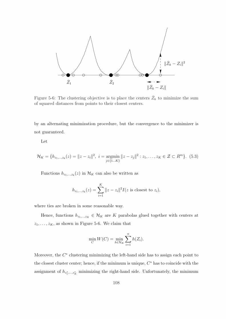
‖Zk − Zi‖2
Z2Z1
‖Zk − Zi‖
Figure 5-6: The clustering objective is to place the centers Zk to minimize the sumof squared distances from points to their closest centers.
by an alternating minimization procedure, but the convergence to the minimizer is
not guaranteed.
Let
HK = hz1,...,zk(z) = ‖z − zi‖2, i = argmin
j∈1...K‖z − zj‖2 : z1, . . . , zK ∈ Z ⊂ Rm. (5.3)
Functions hz1,...,zk(z) in HK can also be written as
hz1,...,zk(z) =
K∑i=1
‖z − zi‖2I(z is closest to zi),
where ties are broken in some reasonable way.
Hence, functions hz1,...,zK∈ HK are K parabolas glued together with centers at
z1, . . . , zK , as shown in Figure 5-6. We claim that
minC
W (C) = minh∈HK
n∑i=1
h(Zi).
Moreover, the C∗ clustering minimizing the left-hand side has to assign each point to
the closest cluster center; hence, if the minimum is unique, C∗ has to coincide with the
assignment of hz∗1 ,...,z∗K minimizing the right-hand side. Unfortunately, the minimum
108

of the empirical average minh∈H∑n
i=1 h(Zi) might not be unique, corresponding to
the scenario depicted in Figures 5-3 and 5-4. In this case, it is interesting to address
the question of stability of this minimization problem.
Let B2(R) denote an L2-ball of radius R, centered at the origin. If Z ⊂ B2(R) for
some constant R, the functions in HK are bounded above by 4R2. Hence, for a fixed
K, the class HK is Donsker. We can apply the result of Corollary 5.4.1 to deduce the
following result.
Theorem 5.7.1. Suppose Z ⊂ B2(R). Let ha1,...,aKand hb1,...,bK
be minimizers of
minh∈HK
n∑i=1
h(Zi)
over the sets S and T , respectively. Here HK is defined as in 5.3. Suppose that
|S 4 T | = o(√
n). Then
‖ha1,...,aK− hb1,...,bK
‖L1(P )P−→ 0.
Stability of ha1,...,aKimplies stability of the centers of the clusters with respect to
perturbation of the data Z1, . . . , Zn.
Definition 5.7.1. Suppose a1, . . . , aK and b1, . . . , bK are centers of two cluster-
ings. Define a “distance” between these clusterings as
dmax(a1, . . . , aK, b1, . . . , bK) := max
(max
imin
j‖ai − bj‖, max
jmin
i‖ai − bj‖
)
Lemma 5.7.1. Assume the measure P is bounded away from 0, i.e. P (z) > c for
some c > 0. Assume further that Z ⊂ B2(0, R) for some R < ∞. Suppose
‖ha1,...,aK− hb1,...,bK
‖L1(P ) ≤ ε.
Then
dmax(a1, . . . , aK, b1, . . . , bK) ≤(
ε
cc,m,R
)1/m
109
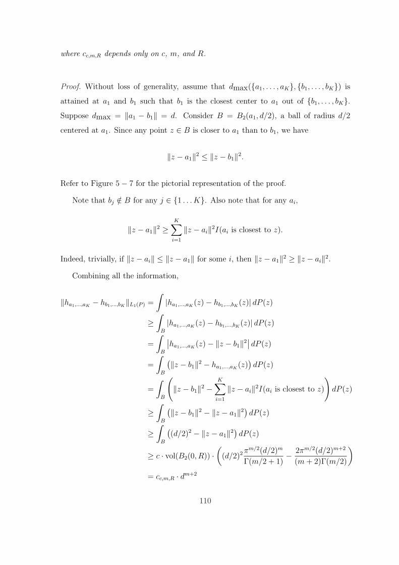
where cc,m,R depends only on c, m, and R.
Proof. Without loss of generality, assume that dmax(a1, . . . , aK, b1, . . . , bK) is
attained at a1 and b1 such that b1 is the closest center to a1 out of b1, . . . , bK.Suppose dmax = ‖a1 − b1‖ = d. Consider B = B2(a1, d/2), a ball of radius d/2
centered at a1. Since any point z ∈ B is closer to a1 than to b1, we have
‖z − a1‖2 ≤ ‖z − b1‖2.
Refer to Figure 5− 7 for the pictorial representation of the proof.
Note that bj /∈ B for any j ∈ 1 . . . K. Also note that for any ai,
‖z − a1‖2 ≥K∑
i=1
‖z − ai‖2I(ai is closest to z).
Indeed, trivially, if ‖z − ai‖ ≤ ‖z − a1‖ for some i, then ‖z − a1‖2 ≥ ‖z − ai‖2.
Combining all the information,
‖ha1,...,aK− hb1,...,bK
‖L1(P ) =
∫|ha1,...,aK
(z)− hb1,...,bK(z)| dP (z)
≥∫
B
|ha1,...,aK(z)− hb1,...,bK
(z)| dP (z)
=
∫
B
∣∣ha1,...,aK(z)− ‖z − b1‖2
∣∣ dP (z)
=
∫
B
(‖z − b1‖2 − ha1,...,aK(z)
)dP (z)
=
∫
B
(‖z − b1‖2 −
K∑i=1
‖z − ai‖2I(ai is closest to z)
)dP (z)
≥∫
B
(‖z − b1‖2 − ‖z − a1‖2)dP (z)
≥∫
B
((d/2)2 − ‖z − a1‖2
)dP (z)
≥ c · vol(B2(0, R)) ·(
(d/2)2 πm/2(d/2)m
Γ(m/2 + 1)− 2πm/2(d/2)m+2
(m + 2)Γ(m/2)
)
= cc,m,R · dm+2
110
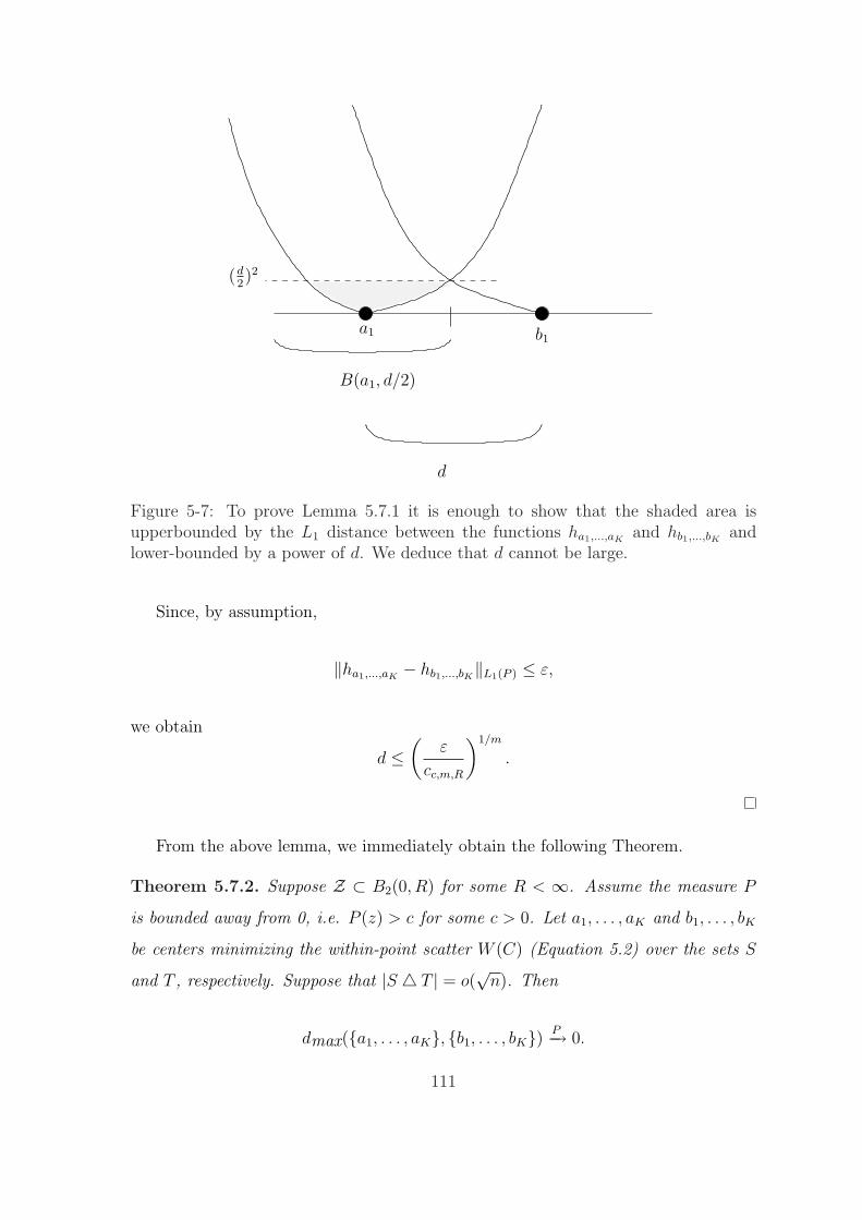
B(a1, d/2)
d
a1 b1
(d2)2
Figure 5-7: To prove Lemma 5.7.1 it is enough to show that the shaded area isupperbounded by the L1 distance between the functions ha1,...,aK
and hb1,...,bKand
lower-bounded by a power of d. We deduce that d cannot be large.
Since, by assumption,
‖ha1,...,aK− hb1,...,bK
‖L1(P ) ≤ ε,
we obtain
d ≤(
ε
cc,m,R
)1/m
.
From the above lemma, we immediately obtain the following Theorem.
Theorem 5.7.2. Suppose Z ⊂ B2(0, R) for some R < ∞. Assume the measure P
is bounded away from 0, i.e. P (z) > c for some c > 0. Let a1, . . . , aK and b1, . . . , bK
be centers minimizing the within-point scatter W (C) (Equation 5.2) over the sets S
and T , respectively. Suppose that |S 4 T | = o(√
n). Then
dmax(a1, . . . , aK, b1, . . . , bK) P−→ 0.
111

Hence, the minimum of the within-point scatter is stable with respect to pertur-
bations of o(√
n) points. Similar results can be obtained for other procedures which
optimize some function of the data by applying Corollary 5.4.1.
5.8 Conclusions
We have presented some new results establishing stability properties of ERM over
certain classes of functions. This study was motivated by the question, raised by
some recent papers, of L1-stability of ERM under perturbations of a single sample
[55, 45, 60]. We gave a partially positive answer to this question, proving that, in
fact, ERM over Donsker classes fulfills L2-stability (and hence also L1-stability) under
perturbations of o(n12 ) among the n samples of the training set. This property follows
directly from the main result which shows decay (in probability) of the diameter of
the set of solutions of almost-ERM with tolerance function ξ(n) = o(n−12 ). We stress
that for classification problems (i.e. for binary-valued functions) no generality is
lost in assuming the Donsker property, since for ERM to be a sound algorithm, the
equivalent Glivenko-Cantelli property has to be assumed anyway. On the other hand,
in the real-valued case, many complexity-based characterizations of Donsker property
are available in the literature.
In the perspective of possible algorithmic applications, we have analyzed some
additional assumptions implying uniform rates of the decay of the L1 diameter of
almost-minimizers. It turned out that an explicit rate of this type can be given for
VC-subgraph classes satisfying a suitable Komlos-Major-Tusnady type condition. For
this condition, many independent characterizations are known. Using a suitable ratio
inequality, we showed how L1-stability results can induce strong forms of expected
error stability, providing a further insight into the behavior of the empirical risk
minimization algorithm.
As in the case of empirical risk minimization, where the geometry of the class
and the underlying measure determine the stability of the minimizers, robustness of
clustering is also related to the number of minimizers of the objective function (i.e.
112

best clusters); we applied our result on the L1-stability of ERM to clustering and the
problem of finding the most/least dense region.
113

114

Chapter 6
Concentration and Stability
In Chapter 3, we proved probabilistic bounds on Remp and Rloo in terms of stability
conditions. The key tools were various deviation and concentration inequalities stated
in Chapter 2.
Recall that the variance of a function of n random variables is small if the function
is not sensitive to changes of each coordinate alone. This corresponds naturally to
the idea of algorithmic stability: the concept learned by the algorithm should not be
sensitive to a change of a training sample. Chapter 3 made the connections between
deviation inequalities and algorithmic stability precise. In the present Chapter, we
provide some further theoretical results on the concentration of functions.
6.1 Concentration of Almost-Everywhere Smooth
Functions
Consider a probability space (Z,G, µ) and the product space (Zn, µn). Let
Tn : Zn 7→ [−1, 1].
We are interested in the connection between the concentration of Tn around its ex-
pectation and the smoothness properties of Tn.
We start with the following definitions.
115

Definition 6.1.1 (Kutin and Niyogi [43]). We say that Tn : Zn 7→ [−1, 1] is strongly
difference-bounded by (β, δ) if there is a subset B ⊂ Zn of measure µn(B) ≤ δ such
that for any 1 ≤ k ≤ n, if ω, ω′ ∈ Zn differ only in the k-th coordinate, then
|Tn(ω)− Tn(ω′)| ≤ β whenever ω /∈ B. (6.1)
We will call B the bad set.
Remark 6.1.1. While in the literature on the concentration of measure phenomenon
the term “concentration” is used in conjunction with exponential bounds on the prob-
ability, we will use this term to denote any convergence of |Tn − ETn| to zero in
probability.
Definition 6.1.2. We will say that Tn concentrates if for any ε > 0
P (|Tn − ETn| > ε) → 0
as n →∞.
Assume that Tn is a bounded function and recall McDiarmid’s inequality (Theorem
2.4.3).
Theorem 6.1.1 (McDiarmid [54]). If Tn : Zn 7→ [−1, 1] is strongly difference-bounded
by (β, 0), then
P (|Tn − ETn| > ε) ≤ 2 exp
(−2ε2
nβ2
)
for any ε > 0.
Hence, Tn concentrates whenever it is strongly difference-bounded by (βn, 0) and
βn = o(n−1/2). We are interested in extensions of McDiarmid’s inequality to non-zero
bad sets, i.e. to functions which are strongly difference-bounded by (βn, δn).
The following extension has been proved by Kutin and Niyogi [43].
116
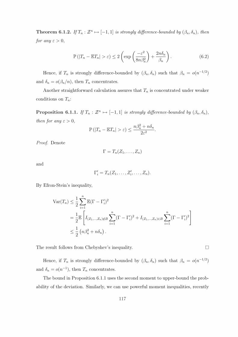
Theorem 6.1.2. If Tn : Zn 7→ [−1, 1] is strongly difference-bounded by (βn, δn), then
for any ε > 0,
P (|Tn − ETn| > ε) ≤ 2
(exp
( −ε2
8nβ2n
)+
2nδn
βn
). (6.2)
Hence, if Tn is strongly difference-bounded by (βn, δn) such that βn = o(n−1/2)
and δn = o(βn/n), then Tn concentrates.
Another straightforward calculation assures that Tn is concentrated under weaker
conditions on Tn:
Proposition 6.1.1. If Tn : Zn 7→ [−1, 1] is strongly difference-bounded by (βn, δn),
then for any ε > 0,
P (|Tn − ETn| > ε) ≤ nβ2n + nδn
2ε2.
Proof. Denote
Γ = Tn(Z1, . . . , Zn)
and
Γ′i = Tn(Z1, . . . , Z′i, . . . , Zn).
By Efron-Stein’s inequality,
Var(Tn) ≤ 1
2
n∑i=1
E(Γ− Γ′i)2
=1
2E
[I(Z1,...,Zn)/∈B
n∑i=1
(Γ− Γ′i)2 + I(Z1,...,Zn)∈B
n∑i=1
(Γ− Γ′i)2
]
≤ 1
2
(nβ2
n + nδn
).
The result follows from Chebyshev’s inequality.
Hence, if Tn is strongly difference-bounded by (βn, δn) such that βn = o(n−1/2)
and δn = o(n−1), then Tn concentrates.
The bound in Proposition 6.1.1 uses the second moment to upper-bound the prob-
ability of the deviation. Similarly, we can use powerful moment inequalities, recently
117
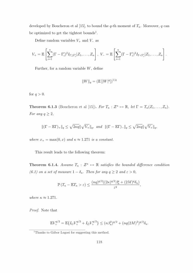
developed by Boucheron et al [15], to bound the q-th moment of Tn. Moreover, q can
be optimized to get the tightest bounds1.
Define random variables V+ and V− as
V+ = E
[n∑
i=1
(Γ− Γ′i)2IΓ≥Γ′i|Z1, . . . , Zn
], V− = E
[n∑
i=1
(Γ− Γ′i)2IΓ<Γ′i|Z1, . . . , Zn
].
Further, for a random variable W , define
‖W‖q = (E [|W |q])1/q
for q > 0.
Theorem 6.1.3 (Boucheron et al [15]). For Tn : Zn 7→ R, let Γ = Tn(Z1, . . . , Zn).
For any q ≥ 2,
‖(Γ− EΓ)+‖q ≤√
2κq‖√
V+‖q, and ‖(Γ− EΓ)−‖q ≤√
2κq‖√
V+‖q,
where x+ = max(0, x) and κ ≈ 1.271 is a constant.
This result leads to the following theorem:
Theorem 6.1.4. Assume Tn : Zn 7→ R satisfies the bounded difference condition
(6.1) on a set of measure 1− δn. Then for any q ≥ 2 and ε > 0,
P (Tn − ETn > ε) ≤ (nq)q/2((2κ)q/2βqn + (2M)qδn)
εq,
where κ ≈ 1.271.
Proof. Note that
EVq/2+ = EIGV
q/2+ + IGV
q/2+ ≤ (nβ2
n)q/2 + (nq(2M)2)q/2δn.
1Thanks to Gabor Lugosi for suggesting this method.
118
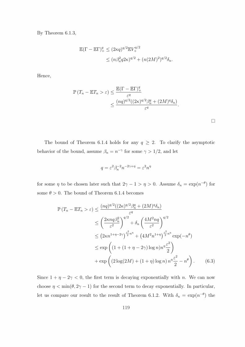
By Theorem 6.1.3,
E(Γ− EΓ)q+ ≤ (2κq)q/2EV
q/2+
≤ (nβ2nq2κ)q/2 + (n(2M)2)q/2δn.
Hence,
P (Tn − ETn > ε) ≤ E(Γ− EΓ)q+
εq
≤ (nq)q/2((2κ)q/2βqn + (2M)qδn)
εq.
The bound of Theorem 6.1.4 holds for any q ≥ 2. To clarify the asymptotic
behavior of the bound, assume βn = n−γ for some γ > 1/2, and let
q = ε2β−2n n−2γ+η = ε2nη
for some η to be chosen later such that 2γ − 1 > η > 0. Assume δn = exp(n−θ) for
some θ > 0. The bound of Theorem 6.1.4 becomes
P (Tn − ETn > ε) ≤ (nq)q/2((2κ)q/2βqn + (2M)qδn)
εq
≤(
2κnqβ2n
ε2
)q/2
+ δn
(4M2nq
ε2
)q/2
≤ (2κn1+η−2γ
) ε2
2nη
+(4M2n1+η
) ε2
2nη
exp(−nθ)
≤ exp
((1 + (1 + η − 2γ) log n)nη ε2
2
)
+ exp
((2 log(2M) + (1 + η) log n) nη ε2
2− nθ
). (6.3)
Since 1 + η − 2γ < 0, the first term is decaying exponentially with n. We can now
choose η < min(θ, 2γ − 1) for the second term to decay exponentially. In particular,
let us compare our result to the result of Theorem 6.1.2. With δn = exp(n−θ) the
119

bound in Equation (6.2) becomes
P (Tn − ETn > ε) ≤ exp
(−ε2
8n2γ−1
)
+ exp((log M + (γ + 1) log n)− nθ
). (6.4)
Depending on whether θ < 2γ − 1 or not, the first or second term dominates conver-
gence to zero, which coincides exactly with the asymptotic behavior of our bound. In
fact, one can verify that the terms in the exponents of bounds (6.3) and (6.4) have
the same order.
We have therefore recovered the result2 of Theorem 6.1.2 for the interesting case
δn = exp(−nθ) by using moment inequality of Boucheron et al [15]. Note that the
result of Theorem 6.1.4 is very general and different ways of picking q might prove
useful. For instance, if δn = 0, i.e. the bounded difference condition (6.1) holds over
the whole Zn, we can choose
q =ε2
4nβ2n
to recover McDiarmid’s inequality.
6.2 The Bad Set
The results of the previous section provide guarantees for the concentration of Tn in
terms of δn and βn. However, not every rate of decay of δn and βn implies that Tn
is concentrated. In fact, this is not due to a weakness in our approach, but rather
due to an apparent phase transition between concentration and non-concentration for
functions of n random variables.
The next example is a negative result: there exists a function Tn with βn = 0 and
δn = Ω(n−1/2) which does not concentrate.
Example 4. Let Z = −1, 1. Let
Tn(Z1, . . . , Zn) = majority(Z1, . . . , Zn).
2This gives an answer to the open question 6.2 in [43].
120
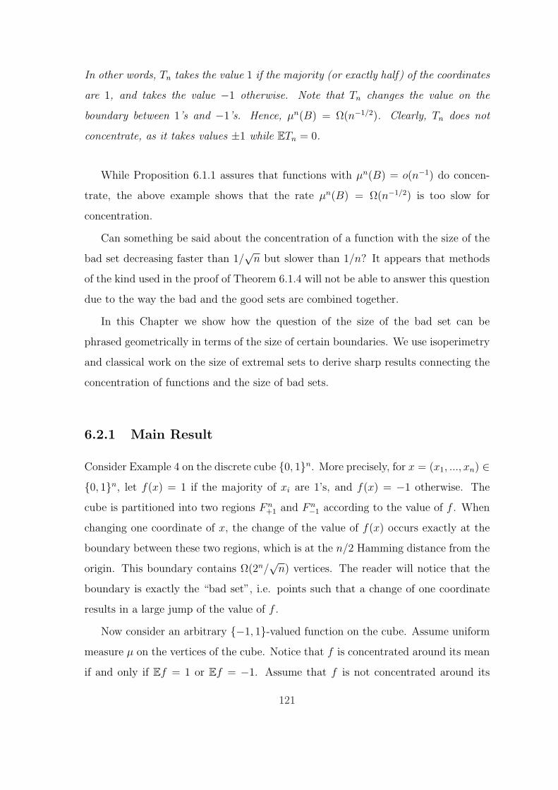
In other words, Tn takes the value 1 if the majority (or exactly half) of the coordinates
are 1, and takes the value −1 otherwise. Note that Tn changes the value on the
boundary between 1’s and −1’s. Hence, µn(B) = Ω(n−1/2). Clearly, Tn does not
concentrate, as it takes values ±1 while ETn = 0.
While Proposition 6.1.1 assures that functions with µn(B) = o(n−1) do concen-
trate, the above example shows that the rate µn(B) = Ω(n−1/2) is too slow for
concentration.
Can something be said about the concentration of a function with the size of the
bad set decreasing faster than 1/√
n but slower than 1/n? It appears that methods
of the kind used in the proof of Theorem 6.1.4 will not be able to answer this question
due to the way the bad and the good sets are combined together.
In this Chapter we show how the question of the size of the bad set can be
phrased geometrically in terms of the size of certain boundaries. We use isoperimetry
and classical work on the size of extremal sets to derive sharp results connecting the
concentration of functions and the size of bad sets.
6.2.1 Main Result
Consider Example 4 on the discrete cube 0, 1n. More precisely, for x = (x1, ..., xn) ∈0, 1n, let f(x) = 1 if the majority of xi are 1’s, and f(x) = −1 otherwise. The
cube is partitioned into two regions F n+1 and F n
−1 according to the value of f . When
changing one coordinate of x, the change of the value of f(x) occurs exactly at the
boundary between these two regions, which is at the n/2 Hamming distance from the
origin. This boundary contains Ω(2n/√
n) vertices. The reader will notice that the
boundary is exactly the “bad set”, i.e. points such that a change of one coordinate
results in a large jump of the value of f .
Now consider an arbitrary −1, 1-valued function on the cube. Assume uniform
measure µ on the vertices of the cube. Notice that f is concentrated around its mean
if and only if Ef = 1 or Ef = −1. Assume that f is not concentrated around its
121

mean and that Ef = 03 . Then, clearly,
µ(F n+1) = µ(F n
−1) = 1/2.
An example of such a function f is depicted in Figure 6-1 below.
−1 −1
−1
+1 +1
+1
+1−1
Figure 6-1: Function f defined at the vertices as −1 or 1 such that Ef = 0.
As in the previous example, the value of f(x) changes only at the boundary
between F n+1 and F n
−1, but this boundary can be more complex than the one in the
previous example (see Figure 6-2). Moreover, by the isoperimetric result of Harper
[31], the extremal set4 of measure 1/2 is exactly the set
x ∈ 0, 1n :n∑
i=1
xi ≤ n/2
i.e. F n−1 of the “majority” example (see Figure 6-3). For more information on extremal
sets see [47], page 31.
Hence, the boundary between two sets of vertices of measure 1/2 has measure
Ω(1/√
n). We therefore have the following theorem:
Theorem 6.2.1. If f : 0, 1n → −1, +1 does not concentrate, then the measure
of the bad set is Ω(1/√
n).
3Throughout this Section we assume, for simplicity, that f is zero-mean, although the proofs arethe same for any non-zero constant mean.
4A set is called extremal if it has the smallest boundary out of sets with the given measure.
122
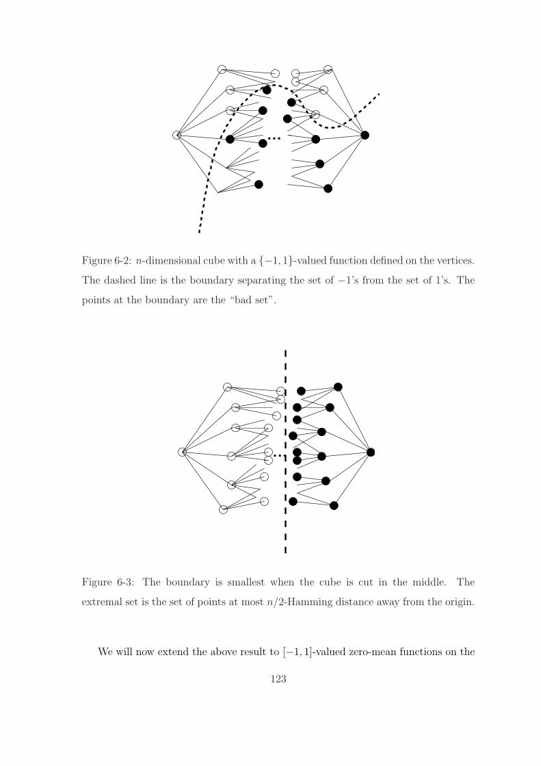
...
Figure 6-2: n-dimensional cube with a −1, 1-valued function defined on the vertices.
The dashed line is the boundary separating the set of −1’s from the set of 1’s. The
points at the boundary are the “bad set”.
...
Figure 6-3: The boundary is smallest when the cube is cut in the middle. The
extremal set is the set of points at most n/2-Hamming distance away from the origin.
We will now extend the above result to [−1, 1]-valued zero-mean functions on the
123
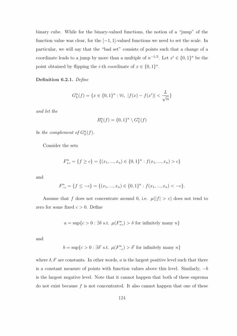
binary cube. While for the binary-valued functions, the notion of a “jump” of the
function value was clear, for the [−1, 1]-valued functions we need to set the scale. In
particular, we will say that the “bad set” consists of points such that a change of a
coordinate leads to a jump by more than a multiple of n−1/2. Let xi ∈ 0, 1n be the
point obtained by flipping the i-th coordinate of x ∈ 0, 1n.
Definition 6.2.1. Define
GnL(f) = x ∈ 0, 1n : ∀i, |f(x)− f(xi)| < L√
n
and let the
BnL(f) = 0, 1n \Gn
L(f)
be the complement of GnL(f).
Consider the sets
F n+c = f ≥ c = (x1, ..., xn) ∈ 0, 1n : f(x1, ..., xn) > c
and
F n−c = f ≤ −c = (x1, ..., xn) ∈ 0, 1n : f(x1, ..., xn) < −c.
Assume that f does not concentrate around 0, i.e. µ(|f | > c) does not tend to
zero for some fixed c > 0. Define
a = supc > 0 : ∃δ s.t. µ(F n+c) > δ for infinitely many n
and
b = supc > 0 : ∃δ′ s.t. µ(F n−c) > δ′ for infinitely many n
where δ, δ′ are constants. In other words, a is the largest positive level such that there
is a constant measure of points with function values above this level. Similarly, −b
is the largest negative level. Note that it cannot happen that both of these suprema
do not exist because f is not concentrated. It also cannot happen that one of these
124
levels is positive while the other supremum does not exist since Ef = 0 and f is
bounded. Thus, a > 0 and b > 0. Let c = min(a, b). By the definition, µ(F n+c) > δ+
and µ(F n−c) > δ−, where δ+ and δ− are constants that depend on c only. Choosing
δc = minδ+, δ−, we obtain
µ(F n+c) > δc and µ(F n
−c) > δc.
The set x : −c < f(x) < c has measure at most 1 − 2δc. Consider slices of
[−c, c]:
Ct =
x : f(x) ∈
[−c + t
L√n
,−c + (t + 1)L√n
]
for t = 0, ...,√
n(2c)L
− 1. These are sets of points on which f takes values within a
L/√
n window. Hence, there exists an interval t0 such that
µ(Ct0) ≤1− 2δc√
n(2c)L
=L(1− 2δc)√
n(2c).
Consider a new (binary-valued) function g : 0, 1n → −1, 1 obtained from f as
follows:
g(x) =
1, if f(x) > −c + (t0 + 1/2) L√n
−1, otherwise
Consider a point x /∈ Ct0 . If a change of any of the coordinates of x results in a
change of the value of g, then the same change of the coordinate results in a change
of the value of f by more than L/√
n. Therefore, the size of the “bad set” of g is
smaller than the size of the bad set of f plus the size of Ct0 :
µ(Bn2 (g)) ≤ µ(Bn
L(f)) + µ(Ct0) ≤ µ(BnL(f)) +
L(1− 2δc)√n(2c)
The result then follows from the Theorem 6.2.1:
Theorem 6.2.2. If f : 0, 1n → [−1, +1] does not concentrate, then there exists an
absolute constant L such that the size of the bad set BnL is Ω(1/
√n).
125

6.2.2 Symmetric Functions
In this section we give an alternate proof for the special case of symmetric functions.
Although the proof of Theorem 6.2.2 is simpler, the following provides some insight
into the geometry of symmetric functions on the binary cube.
The reasoning in this section will be as follows. Assuming that f does not concen-
trate, we will find two sets of constant measure, on which f is “large” positive and
“large” negative, respectively. Next we will show that at least half of each set has to
be within const/√
n Hamming distance from the main diagonal of the cube. This will
imply that Ω(√
n) flips is enough to change a point on which f is large positive into
one on which f is large and negative. In order for this to happen, one of the steps
must be large and that’s what we will call a part of the “bad set”. Due to the nature of
the symmetric functions on the cube, this will imply that a large portion of points is
contained in this “bad set”. This establishes the connection between the concentration
of f and the size of the “bad set”.
Note that the symmetric function f(x1, ..., xn) can take only n values and these
values are determined by the number of 1′s in the bit-string x1, ..., xn. Let
Si = (x1, ..., xn) ∈ 0, 1n :∑
xj = i
and note that f is constant on Si. Since f is symmetric, both F n+c and F n
−c are unions
of Sj’s. Assuming uniform measure, µ(Si) = |Si|/2n. The size |Si| is exactly(
ni
),
while∑n
i=1 |Si| = 2n and µ(Sn/2) = Ω(1/√
n). For x ∈ 0, 1n let |x| denote the
number of 1’s in x (equivalently, Hamming distance from the origin). By definition,
x ∈ S|x|.
Theorem 6.2.3. Assume f : 0, 1n → [−1, 1] is symmetric. If f does not concen-
trate around its mean, there exists an absolute constant L such that the size of the
bad set BnL is at least Ω(1/
√n).
Proof. We define F n+c and F n
+c as in the previous section and recall that µ(F n+c) > δc,
µ(F n−c) > δc. First, we would like to say that at least half of the set F n
+c is within
126

rc
√n Hamming distance from the “main diagonal” Sn/2, where rc is some constant.
From Talagrand’s inequality [47] it follows that
µ
rc√
n⋃i=1
Si
= µ
x : dH(x,
n⋃
j=n/2
Sj) > rc
√n
≤ 1
2e−r2
c .
So,
µ
rc√
n⋃i=1
Si
⋃
n⋃
i=n/2+rc√
n
Si
≤ e−r2
c .
The message of the above inequality is that most of the mass in the cube is concen-
trated around the main diagonal Sn/2. Choosing rc >√
log 2δc
,
µ
rc√
n⋃i=1
Si⋃
n⋃
i=n/2+rc√
n
Si
≤ δc
2
and therefore at least half of F n+c and at least half of F n
−c are within rc
√n Hamming
distance from Sn/2. Denote these subsets by
Hn+c = F n
+c
⋂ x ∈ 0, 1n : |x| ∈ [n/2− rc
√n, n/2 + rc
√n]
and
Hn−c = F n
−c
⋂ x ∈ 0, 1n : |x| ∈ [n/2− rc
√n, n/2 + rc
√n]
.
By the above argument, µ(Hn+c) ≥ δc
2and µ(Hn
−c) ≥ δc
2.
Both Hn+c and Hn
−c are unions of Sj’s and j ∈ [n/2 − rc
√n, n/2 + rc
√n]. Thus,
there must be two indices i, j ∈ [n/2 − rc
√n, n/2 + rc
√n] such that Si ⊂ Hn
+c and
Sj ⊂ Hn−c and by construction, |i− j| ≤ 2rc
√n.
Pick a point x ∈ Si ⊂ Hn+c and change |i − j| coordinates to arrive at some
y ∈ Sj ⊂ Hn−c. Thus, there exists a path of at most 2rc
√n steps from x ∈ Hn
+c
to some y ∈ Hn−c. Note that f(x) > c and f(y) < −c by definition. Therefore,
there is at least one change of a coordinate on this path which results in a jump
of the function value by at least 2c2rc
√n. Assume this jump occurs between some w
127

and wk on the path between x and y, i.e. |f(w) − f(wk)| > crc√
nfor some k. Then
w ∈ Bncrc
. Since f is symmetric, the whole set S|w| belongs to Bncrc
. By construction,
|w| ∈ [n/2 − rc
√n, n/2 + rc
√n]. It then follows that µ(S|w|) = Ω(1/
√n) and thus
µ(Bncrc
) is at least Ω(1/√
n).
6.3 Concentration of Measure: Application of In-
equality of Bobkov-Ledoux
Following Bobkov and Ledoux [12], consider a probability measure µ on a metric
space (Z, d) and a product measure µn on Zn. For g : Zn 7→ R, define
|∇g|(x) = lim supy→x
|g(x)− g(y)|d(x, y)
(6.5)
and let |∇ig| denote the gradient with respect to the ith coordinate. We say that µ
satisfies a Poincare inequality with constant λ if, for every g such that∫
g2dµ < ∞and
∫ |∇g|2dµ < ∞,
λVarµ(g) ≤∫|∇g|2dµ.
Theorem 6.3.1 (Corollary 3.2, [12]). Assume that µ satisfies 6.5 with λ > 0. Then
for every bounded function g on Zn such that
n∑i=1
|∇ig|2 ≤ α2 and maxi≤i≤n
|∇ig| ≤ β
µ-a.e., and for every t ≥ 0
µn
(g ≥
∫fdµn + t
)≤ exp
(− 1
Kmin
(t
β,
t2
α2
))
where K > 0 and only depends on λ > 0.
For S = Z1, . . . , Zn, let fS be an (approximate) empirical minimizer over F .
Similarly, fT is an (approximate) empirical minimizer for the set T = Z ′1, ..., Z
′k.
128

We will apply the concentration result of Theorem 6.3.1 to
g(Z1, . . . , Zn) =1
n
n∑i=1
fS(zi).
To do so, we need to show that g is smooth.
Note that if S and T differ only in the ith sample,
∣∣∣∣∣1
n
∑z∈S
fS(z)− 1
n
∑z∈T
fT (z)
∣∣∣∣∣ ≤L
nd(zi, z
′i)
by a proof similar to that of Corollary 5.4.2. Hence,
|∇ig| ≤ L
n.
Now, assume µ satisfies the Poincare inequality with λ > 0. We now apply
Theorem 6.3.1 to the function g : Zn 7→ [−2, 2] with α2 = L2
nand β = L
n. We obtain
P (g ≥ Eg + t) ≤ exp
(− 1
Kmin
(nt
L,nt2
L2
)).
By applying the concentration inequality to −g we can obtain the two-sided inequal-
ity:
P (|g − Eg| ≥ t) ≤ 2 exp
(− 1
Kmin
(nt
L,nt2
L2
)).
Note that Eg is a constant which depends on the problem.
Theorem 6.3.2. Assume µ satisfies the Poincare inequality with λ > 0 and that all
functions f ∈ F are Lipschitz with a constant L. For any δ > 0 and n > K log 2δ,
∣∣∣∣∣1
n
n∑i=1
fS(zi)− φn
∣∣∣∣∣ ≤KL log 2
δ
n
with probability at least 1− δ. Here φn = ESfS(z1) is a data-independent quantity
and K depends on λ.
The Poincare condition on the measure µ is fairly restrictive, as it allows such
129

tight concentration of empirical errors. In particular, it follows that for independent
draws of S and T ,
∣∣∣∣∣1
n
∑z∈S
fS(z)− 1
n
∑z∈T
fT (z)
∣∣∣∣∣ ≤KL log 2
δ
n
with probability at least 1− 2δ. Hence, the empirical errors of empirical minimizers
over different samples are very close to each other with high probability. Such behavior
has been observed by Boucheron et al [14] (Theorem 19) and others, although under
different complexity conditions on the function class.
130

Appendix A
Technical Proofs
In this appendix we derive some results presented in Section 5.3. In particular, we
prove Lemma 5.3.1, which was used in the proof of Theorem 5.3.1, and Corollary
5.3.1. Let us start with some technical Lemmas.
Lemma A.0.1. Let f0, f1 ∈ F , ‖f0 − f1‖ ≥ C/2, ‖f1‖ ≤ ‖f0‖. Let h : F → R be
defined as h(f ′) = 〈f ′,f0〉‖f0‖2 . Then for any ε ≤ C3
128
infB(f0,ε)
h− supB(f1,ε)
h ≥ C2
16.
Proof.
∆ := infB(f0,ε)
h− supB(f1,ε)
h
= h(f0)− h(f1) + infh(f ′ − f0) + h(f1 − f ′′)|f ′ ∈ B(f0, ε), f′′ ∈ B(f1, ε)
≥ h(f0)− h(f1)− 2ε
‖f0‖ ≥ h(f0)− h(f1)− 8ε
C,
since ‖f0‖ ≥ C/4.
Finally
2 〈f0 − f1, f0〉 = ‖f0 − f1‖2 − ‖f1‖2 + ‖f0‖2 ≥ ‖f0 − f1‖2 ≥ C2
4,
131

then
h(f0)− h(f1) ≥ C2
8 ‖f0‖2 ≥C2
8,
which proves that
∆ ≥ C2
8− 8ε
C≥ C2
16.
The following Lemma is an adaptation of Lemma 2.3 of [37].
Lemma A.0.2. Let f0, f1, h be defined as in Lemma A.0.1. Suppose ε ≤ C3
128. Let νµ
be a Gaussian process on F with mean µ and covariance cov(νµ(f), νµ(f ′)) = 〈f, f ′〉.Then for all δ > 0
Pr∗(| supB(f0,ε)
νµ − supB(f1,ε)
νµ| ≤ δ
)≤ 64δ
C3.
Proof. Define the Gaussian process Y (·) = νµ(·)− h(·)νµ(f0). Since
cov(Y (f ′), νµ(f0)) = 〈f ′, f0〉 − h(f ′) ‖f0‖2 = 0,
νµ(f0) and Y (·) are independent.
We now reason conditionally with respect to Y (·). Define
Γi(z) = supB(fi,ε)
Y (·) + h(·)z with i = 0, 1.
Notice that
Pr∗(| supB(f0,ε)
νµ − supB(f1,ε)
νµ| ≤ δ|Y)
= Pr∗ (|Γ0(νµ(f0))− Γ1(νµ(f0))| ≤ δ) .
132

Moreover Γ0 and Γ1 are convex and
inf ∂−Γ0 − sup ∂+Γ1 ≥ infB(f0,ε)
h− supB(f1,ε)
h ≥ C2
16,
by Lemma A.0.1. Then Γ0 = Γ1 in a single point z0 and
Pr∗ (|Γ0(νµ(f0))− Γ1(νµ(f0))| ≤ δ) ≤ Pr∗ (νµ(f0) ∈ [z0 −∆, z0 + ∆]) ,
with ∆ = 16δ/C2.
Furthermore,
Pr∗ (νµ(f0) ∈ [z0 −∆, z0 + ∆]) ≤ 32δ
C2√
2πvar(νµ(f0)),
and var(νµ(f0)) = ‖f0‖2 ≥ C2/16, which completes the proof.
The reasoning in the proof of the next lemma goes as follows. We consider a finite
cover of F . Pick any two almost-minimizers which are far apart. They belong to two
covering balls with centers far apart. Because the two almost-minimizers belong to
these balls, the infima of the empirical risks over these two balls are close. This is
translated into the event that the suprema of the shifted empirical process over these
two balls are close. By looking at the Gaussian limit process, we are able to exploit
the covariance structure to show that the suprema of the Gaussian process over balls
with centers far apart are unlikely to be close.
Lemma 5.3.1. Consider the ε-covering fi|i = 1, . . . ,N (ε,F , ‖·‖). Such a covering
exists because F is totally bounded in ‖·‖ norm [see page 89, 71]. For any f, f ′ ∈MξS
s.t. ‖f − f ′‖ > C, there exist k and l such that ‖f − fk‖ ≤ ε ≤ C/4, ‖f ′ − fl‖ ≤ ε ≤C/4. By triangle inequality it follows that ‖fk − fl‖ ≥ C/2.
Moreover
infF
Pn ≤ infB(fk,ε)
Pn ≤ Pnf ≤ infF
Pn + ξ
133

and
infF
Pn ≤ infB(fl,ε)
Pn ≤ Pnf ′ ≤ infF
Pn + ξ.
Therefore, ∣∣∣∣ infB(fk,ε)
Pn − infB(fl,ε)
Pn
∣∣∣∣ ≤ ξ.
The last relation can be restated in terms of the empirical process νn:
∣∣∣∣∣ supB(fk,ε)
−νn −√
nP − supB(fl,ε)
−νn −√
nP∣∣∣∣∣ ≤ ξ
√n ≤ δ.
Now,
Pr∗(diamMξ
S > C)
= Pr∗(∃f, f ′ ∈Mξ
S, ‖f − f ′‖ > C)≤
Pr∗(∃l, k s.t. ‖fk − fl‖ ≥ C/2,
∣∣∣∣∣ supB(fk,ε)
−νn −√
nP − supB(fl,ε)
−νn −√
nP∣∣∣∣∣ ≤ δ
).
By union bound
Pr∗(diamMξ
S > C)
≤N (ε,F ,‖·‖)∑
k,l=1‖fk−fl‖≥C/2
Pr∗(∣∣∣∣∣ sup
B(fk,ε)
−νn −√
nP − supB(fl,ε)
−νn −√
nP∣∣∣∣∣ ≤ δ
).
We now want to bound the terms in the sum above. Assuming without loss of
generality that ‖fk‖ ≥ ‖fl‖, we obtain
Pr∗(∣∣∣∣∣ sup
B(fk,ε)
−νn −√
nP − supB(fl,ε)
−νn −√
nP∣∣∣∣∣ ≤ δ
)
= Pr∗(∣∣∣∣∣ sup
B(fk,ε)
−ν ′n −√
nP − supB(fl,ε)
−ν ′n −√
nP∣∣∣∣∣ ≤ δ
)
= Pr∗(∣∣∣∣∣ sup
B(fk,ε)
−ν ′ −√nP + ν ′ − ν ′n − supB(fl,ε)
−ν ′ −√nP + ν ′ − ν ′n∣∣∣∣∣ ≤ δ
)
134

≤ Pr∗(∣∣∣∣∣ sup
B(fk,ε)
−ν ′ −√nP − supB(fl,ε)
−ν ′ −√nP∣∣∣∣∣ ≤ 2δ
)
+ Pr∗(
supF|ν ′n − ν ′| ≥ δ/2
)
≤ 128δ
C3+ Pr∗
(supF|ν ′n − ν ′| ≥ δ/2
),
where the first inequality results from a union bound argument while the second
one results from Lemma A.0.2 noticing that −ν ′ −√nP is a Gaussian process with
covariance 〈f, f ′〉 and mean −√nP , and since by construction ε ≤ C3/128.
Finally, the claimed result follows from the two last relations.
We now prove, Corollary 5.3.1, the extension of Theorem 5.3.1 to L2 diameters.
The proof relies on the observation that a P -Donsker class is also Glivenko-Cantelli.
Corollary 5.3.1. Note that
‖f − f ′‖2L2
= ‖f − f ′‖2+ (P (f − f ′))2
.
The expected errors of almost-minimizers over a Glivenko-Cantelli (and therefore
over Donsker) class are close because empirical averages uniformly converge to the
expectations.
Pr∗(∃f, f ′ ∈Mξ(n)
S s.t. ‖f − f ′‖L2> C
)
≤ Pr∗(∃f, f ′ ∈Mξ(n)
S s.t. |Pf − Pf ′| > C/√
2)
+ Pr∗(diamMξ(n)
S > C/√
2)
.
The first term can be bounded as
Pr∗(∃f, f ′ ∈Mξ(n)
S s.t. |Pf − Pf ′| > C/√
2)
≤ Pr∗(∃f, f ′ ∈ F , |Pnf − Pnf
′| ≤ ξ(n), |Pf − Pf ′| > C/√
2)
≤ Pr∗(
supf,f ′∈F
|(Pn − P )(f − f ′)| > |C/√
2− ξ(n)|)
which goes to 0 because the class f − f ′|f, f ′ ∈ F is Glivenko-Cantelli. The second
135
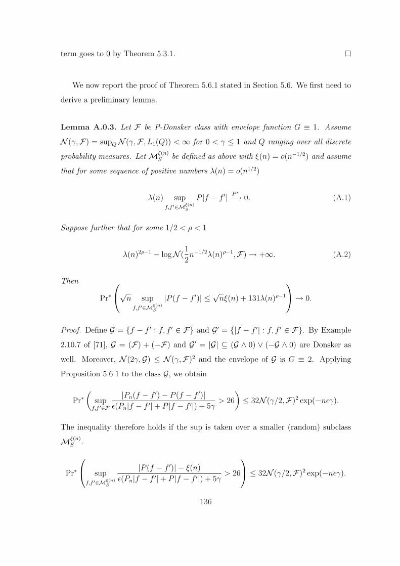
term goes to 0 by Theorem 5.3.1.
We now report the proof of Theorem 5.6.1 stated in Section 5.6. We first need to
derive a preliminary lemma.
Lemma A.0.3. Let F be P-Donsker class with envelope function G ≡ 1. Assume
N (γ,F) = supQN (γ,F , L1(Q)) < ∞ for 0 < γ ≤ 1 and Q ranging over all discrete
probability measures. Let Mξ(n)S be defined as above with ξ(n) = o(n−1/2) and assume
that for some sequence of positive numbers λ(n) = o(n1/2)
λ(n) supf,f ′∈Mξ(n)
S
P |f − f ′| P ∗−→ 0. (A.1)
Suppose further that for some 1/2 < ρ < 1
λ(n)2ρ−1 − logN (1
2n−1/2λ(n)ρ−1,F) → +∞. (A.2)
Then
Pr∗
√n sup
f,f ′∈Mξ(n)S
|P (f − f ′)| ≤ √nξ(n) + 131λ(n)ρ−1
→ 0.
Proof. Define G = f − f ′ : f, f ′ ∈ F and G ′ = |f − f ′| : f, f ′ ∈ F. By Example
2.10.7 of [71], G = (F) + (−F) and G ′ = |G| ⊆ (G ∧ 0) ∨ (−G ∧ 0) are Donsker as
well. Moreover, N (2γ,G) ≤ N (γ,F)2 and the envelope of G is G ≡ 2. Applying
Proposition 5.6.1 to the class G, we obtain
Pr∗(
supf,f ′∈F
|Pn(f − f ′)− P (f − f ′)|ε(Pn|f − f ′|+ P |f − f ′|) + 5γ
> 26
)≤ 32N (γ/2,F)2 exp(−nεγ).
The inequality therefore holds if the sup is taken over a smaller (random) subclass
Mξ(n)S .
Pr∗
sup
f,f ′∈Mξ(n)S
|P (f − f ′)| − ξ(n)
ε(Pn|f − f ′|+ P |f − f ′|) + 5γ> 26
≤ 32N (γ/2,F)2 exp(−nεγ).
136
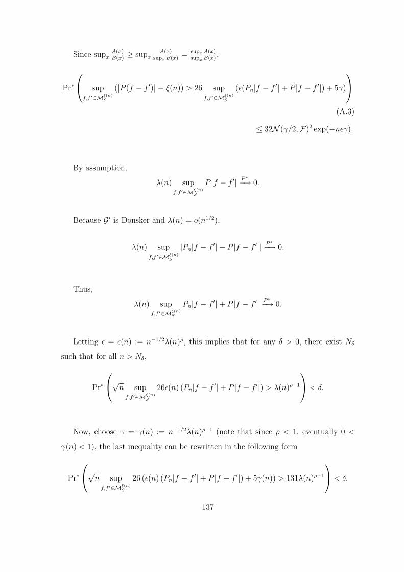
Since supxA(x)B(x)
≥ supxA(x)
supx B(x)= supx A(x)
supx B(x),
Pr∗
sup
f,f ′∈Mξ(n)S
(|P (f − f ′)| − ξ(n)) > 26 supf,f ′∈Mξ(n)
S
(ε(Pn|f − f ′|+ P |f − f ′|) + 5γ)
(A.3)
≤ 32N (γ/2,F)2 exp(−nεγ).
By assumption,
λ(n) supf,f ′∈Mξ(n)
S
P |f − f ′| P ∗−→ 0.
Because G ′ is Donsker and λ(n) = o(n1/2),
λ(n) supf,f ′∈Mξ(n)
S
|Pn|f − f ′| − P |f − f ′|| P ∗−→ 0.
Thus,
λ(n) supf,f ′∈Mξ(n)
S
Pn|f − f ′|+ P |f − f ′| P ∗−→ 0.
Letting ε = ε(n) := n−1/2λ(n)ρ, this implies that for any δ > 0, there exist Nδ
such that for all n > Nδ,
Pr∗
√n sup
f,f ′∈Mξ(n)S
26ε(n) (Pn|f − f ′|+ P |f − f ′|) > λ(n)ρ−1
< δ.
Now, choose γ = γ(n) := n−1/2λ(n)ρ−1 (note that since ρ < 1, eventually 0 <
γ(n) < 1), the last inequality can be rewritten in the following form
Pr∗
√n sup
f,f ′∈Mξ(n)S
26 (ε(n) (Pn|f − f ′|+ P |f − f ′|) + 5γ(n)) > 131λ(n)ρ−1
< δ.
137

Combining the relation above with Eqn. A.3,
Pr∗
√n sup
f,f ′∈Mξ(n)S
|P (f − f ′)| ≤ √nξ(n) + 131λ(n)ρ−1
≥ 1− 32N(
1
2n−1/2λ(n)ρ−1,F
)2
exp(−λ(n)2ρ−1)− δ.
The result follows by the assumption on the entropy and by arbitrariness of δ.
We are now ready to prove Theorem 5.6.1.
Theorem 5.6.1. By Corollary 5.5.1,
nγdiamMξ(n)S
P ∗−→ 0
for any γ < min(
13(2V +1)
min(α, η), 1/2). Let λ(n) = nγ and note that λ(n) = o(
√n),
which is a condition in Lemma A.0.3. First, we show that a power decay of the ‖·‖diameter implies the same rate of decay of the L1 diameter, hence verifying condition
(A.1) in Lemma A.0.3. Proof of this fact is very similar to the proof of Corollary
5.3.1, except that C is replaced by Cλ(n)−1.
Pr∗(∃f, f ′ ∈Mξ(n)
S s.t. ‖f − f ′‖L2> Cλ(n)−1
)
≤ Pr∗(∃f, f ′ ∈Mξ(n)
S s.t. |Pf − Pf ′| > Cλ(n)−1/√
2)
+ Pr∗(diamMξ(n)
S > Cλ(n)−1/√
2)
.
The second term goes to zero since λ(n)diamMξ(n)S
P ∗−→ 0. Moreover, since λ(n) =
138

o(√
n) and G is Donsker, the first term can be bounded as
Pr∗(∃f, f ′ ∈Mξ(n)
S s.t. |Pf − Pf ′| > Cλ(n)−1/√
2)
≤ Pr∗(∃f, f ′ ∈ F , |Pnf − Pnf
′| ≤ ξ(n), |Pf − Pf ′| > Cλ(n)−1/√
2)
≤ Pr∗(
supf,f ′∈F
|P (f − f ′)− Pn(f − f ′)| >∣∣∣∣
C√2λ(n)−1 − ξ(n)
∣∣∣∣)
= Pr∗(
λ(n) supg∈G
|Pg − Png| >∣∣∣∣
C√2− ξ(n)λ(n)
∣∣∣∣)→ 0,
proving condition (A.1) in Lemma A.0.3.
We now verify condition (A.2) in Lemma A.0.3. Since F is a VC-subgraph class of
dimension V , its entropy numbers logN (ε,F) behave like V log Aε
(A is a constant),
that is
logN(
1
2n−1/2λ(n)ρ−1,F
)≤ const +
1
2V log n + (1− ρ)V log λ(n).
Condition (A.2) of Lemma A.0.3 will therefore hold whenever λ(n) grows faster than
(log n)1
2ρ−1 , for any 1 > ρ > 12. In our problem, λ(n) grows polynomially, so condition
(A.2) is satisfied for any fixed 1 > ρ > 1/2.
Hence, by Lemma A.0.3
Pr∗
√n sup
f,f ′∈Mξ(n)S
|P (f − f ′)| ≤ √nξ(n) + 131nγ(ρ−1)
→ 0.
Choose any 0 < κ < γ/2 and multiply both sides of the inequality by nκ. We obtain
Pr∗
nκ
√n sup
f,f ′∈Mξ(n)S
|P (f − f ′)| ≤ √nξ(n)nκ + 131nγ(ρ−1)+κ
→ 0. (A.4)
Now fix a ρ such that 1/2 < ρ < 1− κ/γ. Because 0 < κ < γ/2, there is always such
a choice of ρ. Furthermore, 1 > ρ > 1/2 so that the above convergence holds. Our
choice of ρ implies that γ(ρ − 1) + κ < 0 and so nγ(ρ−1)+κ → 0. Since κ < γ/2 < η,
139

√nξ(n)nκ → 0. Hence,
n1/2+κ supf,f ′∈Mξ(n)
S
|P (f − f ′)| P ∗−→ 0
for any κ < min(
16(2V +1)
min(α, η), 1/2).
140
Bibliography
[1] N. Alon, S. Ben-David, N. Cesa-Bianchi, and D. Haussler. Scale-sensitive di-
mensions, uniform convergnce, and learnability. J. of the ACM, 44(4):615–631,
1997.
[2] S. Arora, L. Babai, J. Stern, and Z. Sweedyk. Hardness of approximate optima
in lattices, codes, and linear systems. Journal of Computer and System Sciences,
54(2):317–331, 1997.
[3] A.R. Barron. Universal approximation bounds for superpositions of a sigmoidal
function. IEEE Transaction on Information Theory, 39(3):930–945, May 1993.
[4] A.R. Barron. Approximation and estimation bounds for artificial neural net-
works. Machine Learning, 14:115–133, 1994.
[5] Peter L. Bartlett, Michael I. Jordan, and Jon D. McAuliffe. Convexity, classifi-
cation, and risk bounds. Journal of the American Statistical Association, 2005.
To appear.
[6] Peter L. Bartlett and Shahar Mendelson. Empirical minimization. Probability
Theory and Related Fields, 2005. To appear.
[7] Peter L. Bartlett, Shahar Mendelson, and PetraPhilips. Local complexities
for empirical risk minimization. In Proceedings of the 17th Annual Conference
on Computational Learning Theory (COLT2004), volume 3120, pages 270–284.
Springer, 2004.
141

[8] Peter L. Bartlett, Shahar Mendelson, and PetraPhilips. Optimal sample-based
estimates of the expectation of the empirical minimizer. Submitted., 2005.
[9] S. Ben-David, N. Eiron, and P. M. Long. On the difficulty of approximately
maximizing agreements. Journal of Computer and System Sciences, 66(3):496–
514, 2003.
[10] G. Bennett. Probability inequalities for sums of independent random variables.
Journal of the American Statistical Association, 57:33–45, 1962.
[11] L. Birge and P. Massart. Rates of convergence for minimum contrast estimators.
Probability Theory and Related Fields, 97:113–150, 1993.
[12] S. Bobkov and M. Ledoux. Poincare’s inequalities and talagrand’s concentration
phenomenon for the exponential distribution. Probability Theory and Related
Fields, 107:383–400, 1997.
[13] S. Boucheron, O. Bousquet, and G. Lugosi. Concentration Inequalities, pages
208–240. springer, 2004.
[14] S. Boucheron, G. Lugosi, and P. Massart. Concentration inequalities using the
entropy method. The Annals of Probability, 31:1583–1614, 2003.
[15] Stephane Boucheron, Olivier Bousquet, Gabor Lugosi, and Pascal Massart. Mo-
ment inequalities for functions of independent random variables. The Annals of
Probability, 33(2):514–560, 2005.
[16] Olivier Bousquet and Andre Elisseeff. Stability and generalization. Journal of
Machine Learning Research, 2:499–526, 2002.
[17] L. Breiman. Bagging predictors. Machine Learning, 26(2):123–140, 1996.
[18] A. Caponnetto and A. Rakhlin. Some properties of empirical risk minimization
over Donsker classes. Available at http://cbcl.mit.edu/people/rakhlin/erm.pdf.
Submitted to JMLR, 2005.
142

[19] A. Caponnetto and A. Rakhlin. Some properties of empirical risk minimization
over donsker classes. AI Memo 2005-018, Massachusetts Institute of Technology,
May 2005.
[20] L. Devroye, L. Gyorfi, and G. Lugosi. A Probabilistic Theory of Pattern Recog-
nition. Number 31 in Applications of mathematics. Springer, New York, 1996.
[21] L. Devroye and T. Wagner. Distribution-free probability inequalities for the
deleted and holdout estimates. IEEE Transactions on Information Theory,
25:202–207, 1979.
[22] L.P. Devroye and T.J. Wagner. Distribution-free performance bounds for poten-
tial function rules. IEEE Transactions on Information Theory, 25(5):601–604,
1979.
[23] L.P. Devroye and T.J. Wagner. Distribution-free consistency results in non-
parametric discrimination and regression function estimation. The Annals of
Statistics, 8:231–239, 1980.
[24] R. O. Duda and P. E. Hart. Pattern Classification and Scene Analysis. Wiley,
New York, 1973.
[25] Richard M. Dudley. Uniform Central Limit Theorems. Cambridge University
Press, 1999.
[26] B. Efron and C. Stein. The jackknife estimate of variance. The Annals of
Statistics, 9(3):586–596, 1981.
[27] Y. Freund and R. Schapire. A short introduction to boosting. Journal of Japanese
Society for Artificial Intelligence, 14(5):771–780, 1999.
[28] E. Gine and J. Zinn. Some limit theorems for empirical processes. The Annals
of Probability, 12(4):929–989, 1984.
[29] E. Gine and J. Zinn. Gaussian characterization of uniform Donsker classes of
functions. The Annals of Probability, 19:758–782, 1991.
143

[30] L. S. Gottfredson. Mainstream science on intelligence: An editorial with 52
signatories, history, and bibliography. Intelligence, 24(1):13–23, 1997.
[31] L.H. Harper. Optimal numberings and isoperimetric problems on graphs. Journal
of Combinatorial Theory, 1:385–393, 1966.
[32] T. Hastie and R. Tibshirani. Generalized Additive Models, volume 43 of Mono-
graphs on Statistics and Applied Probability. Chapman and Hall, London, 1990.
[33] Trevor Hastie, Robert Tibshirani, and Jerome Friedman. The Elements of Sta-
tistical Learning - Data Mining, Inference, and Prediction. Springer, 2002. HAS
t 01:1 1.Ex.
[34] W. Hoeffding. Probability inequalities for sums of bounded random variables.
Journal of the American Statistical Association, 58(301):13–30, 1963.
[35] L.K. Jones. A simple lemma on greedy approximation in Hilbert space and
convergence rates for Projection Pursuit Regression and neural network training.
The Annals of Statistics, 20(1):608–613, March 1992.
[36] M. J. Kearns and D. Ron. Algorithmic stability and sanity-check bounds for
leave-one-out cross-validation. In Proceedings of the Tenth Annual Conference
on Computational Learning Theory (COLT), pages 152–162. ACM Press, New
York, 1997.
[37] J. Kim and D. Pollard. Cube root asymptotics. Annals of Statistics, 18:191–219,
1990.
[38] V. Koltchinskii. Local Rademacher complexities and oracle inequalities in risk
minimization. Technical report, University of New Mexico, August 2003.
[39] V. Koltchinskii and D. Panchenko. Rademacher processes and bounding the risk
of function learning. High Dimensional Probability, II:443–459, 2000.
144

[40] V. Koltchinskii and D. Panchenko. Empirical margin distributions and bounding
the generalization error of combined classifiers. The Annals of Statistics, 30(1):1–
50, 2002.
[41] V. Koltchinskii, D. Panchenko, and F. Lozano. Bounding the generalization
error of convex combinations of classifiers: balancing the dimensionality and the
margins. Annals of Applied Probability, 13(1):213–252, 2003.
[42] Vladimir I. Koltchinskii. Komlos-Major-Tusnady approximation for the general
empirical process and Haar expansion of classes of functions. Journal of Theo-
retical Probability, 7:73–118, 1994.
[43] S. Kutin. Extensions to mcdiarmid’s inequality when differences are bounded
with high probability. Technical report TR-2002-04, University of Chicago, 2002.
[44] S. Kutin and P. Niyogi. Almost-everywhere algorithmic stability and generaliza-
tion error. Technical report TR-2003-03, University of Chicago, 2002.
[45] Samuel Kutin and Partha Niyogi. Almost-everywhere algorithmic stability and
generalization error. In UAI, pages 275–282, 2002.
[46] M. Ledoux and M. Talagrand. Probability in Banach Spaces. Springer-Verlag,
New York, 1991.
[47] Michael Ledoux. The Concentration of Measure Phenomenon, volume 89 of
Mathematical Surveys and Monographs. American Mathematical Society, 2001.
[48] W. S. Lee, P. L. Bartlett, and R. C. Williamson. The importance of convex-
ity in learning with squared loss. IEEE Transactions on Information Theory,
44(5):1974–1980, 1998.
[49] J. Li and A. Barron. Mixture density estimation. In S. A. Solla, T. K. Leen,
and K.-R. Muller, editors, Advances in Neural information processings systems
12, San Mateo, CA, 1999. Morgan Kaufmann Publishers.
145
[50] Jonathan Q. Li. Estimation of Mixture Models. PhD thesis, The Department of
Statistics. Yale University, 1999.
[51] G. Lugosi and N. Vayatis. On the Bayes-risk consistency of regularized boosting
methods. The Annals of Statistics, 32(1):30–55, 2004.
[52] Shie Mannor, Ron Meir, and Tong Zhang. The consistency of greedy algorithms
for classification. In COLT, pages 319–333, 2002.
[53] Shie Mannor, Ron Meir, and Tong Zhang. Greedy algorithms for classification
– consistency, convergence rates, and adaptivity. Journal of Machine Learning
Research, 4:713–741, 2003.
[54] C. McDiarmid. On the method of bounded differences. In Surveys in Combina-
torics, London Math. Soc. Lect. Note Series 141, pages 148–188, 1989.
[55] S. Mukherjee, P. Niyogi, T. Poggio, and R. Rifkin. Statistical learning: Stability
is necessary and sufficient for consistency of empirical risk minimization. CBCL
Paper 2002-023, Massachusetts Institute of Technology, December 2002 [January
2004 revision].
[56] P. Niyogi and F. Girosi. Generalization bounds for function approximation from
scattered noisy data. Advances in Computational Mathematics, 10:51–80, 1999.
[57] T. Poggio and F. Girosi. Networks for approximation and learning. Proceedings
of the IEEE, 78(9), September 1990.
[58] T. Poggio, T. Rifkin, R. Mukherjee S., and P. Niyogi. General conditions for
predictivity in learning theory. Nature, pages 419–422, 2004.
[59] D. Pollard. Uniform ratio limit theorems for empirical processes. Scandinavian
Journal of Statistics, 22(3):271–278, 1995.
[60] A. Rakhlin, S. Mukherjee, and T. Poggio. Stability results in learning theory.
Analysis and Applications, 3(4):397–419, 2005.
146

[61] A. Rakhlin, D. Panchenko, and S. Mukherjee. Risk bounds for mixture density
estimation. ESAIM: Probability and Statistics, 9:220–229, 2005.
[62] E. Rio. Strong approximation for set-indexed partial sum processes via KMT
constructions I. The Annals of Probability, 21(2):759–790, 1993.
[63] W. H. Rogers and T. J. Wagner. A finite sample distribution-free performance
bound for local discrimination rules. The Annals of Statistics, 6(3):506–514,
1978.
[64] M. Rudelson and R. Vershynin. Combinatorics of random processes and sections
of convex bodies. Annals of Mathematics. To appear.
[65] R. Schapire. A brief introduction to boosting. In Proceedings of the Sixteenth
International Joint Conference on Artificial Intelligence, pages 1401–1406, 1999.
[66] R. E. Schapire. The strength of weak learnability. Machine Learning, 5(2):197–
227, 1990.
[67] M. Talagrand. Sharper bounds for Gaussian and empirical processes. The Annals
of Probability, 22:20–76, 1994.
[68] A. N. Tikhonov and V. Y. Arsenin. Solutions of Ill-posed Problems. W. H.
Winston, Washington, D.C., 1977.
[69] S.A. van de Geer. Rates of convergence for the maximum likelihood estimator
in mixture models. Nonparametric Statistics, 6:293–310, 1996.
[70] S.A. van de Geer. Empirical Processes in M-Estimation. Cambridge University
Press, 2000.
[71] A. W. van der Vaart and J. A. Wellner. Weak Convergence and Empirical Pro-
cesses with Applications to Statistics. Springer-Verlag, New York, 1996.
[72] V. Vapnik. The Nature of Statistical Learning Theory. Springer, New York, 1995.
147

[73] V. N. Vapnik. An overview of statistical learning theory. IEEE Transactions on
Neural Networks, 10(5):988–99, 1999.
[74] V. N. Vapnik and A. Y. Chervonenkis. On the uniform convergence of rela-
tive frequencies of events to their probabilities. Theory of Probability and Its
Applications, 16(2):264–280, 1971.
[75] V.N. Vapnik and A. Ya. Chervonenkis. The necessary and sufficient conditions
for the uniform convergence of averages to their expected values. Teoriya Veroy-
atnostei i Ee Primeneniya, 26(3):543–564, 1981.
[76] V.N. Vapnik and A. Ya. Chervonenkis. The necessary and sufficient conditions
for consistency in the empirical risk minimization method. Pattern Recognition
and Image Analysis, 1(3):283–305, 1991.
[77] G. Wahba. Splines Models for Observational Data. Series in Applied Mathemat-
ics, Vol. 59, SIAM, Philadelphia, 1990.
[78] W.H. Wong and X. Shen. Probability inequalities for likelihood ratios and con-
vergence rates for sieve mles. Annals of Statistics, 23:339–362, 1995.
[79] T. Zhang. Statistical behavior and consistency of classification methods based
on convex risk minimization. The Annals of Statistics, 32(1):56–85, 2004.
[80] Tong Zhang. Sequential greedy approximation for certain convex optimization
problems. IEEE Transactions on Information Theory, 49(3):682–691, 2003.
148


![Atmospheric Processes Governing the Northern Hemisphere ...davet/ao/Thompson...1 Atmospheric Processes Governing the Northern Hemisphere ... 1981] or rotated empirical orthogonal functions](https://img.pdfslide.us/doc/110x75/602df21aea1b56338f4a1953/atmospheric-processes-governing-the-northern-hemisphere-davetaothompson.jpg)