Applications of Differential Geometry to Mathematical Physics · Ste en Krusch Applications of Di erential Geometry to Mathematical Physics. More on sections Vector bundles always

Applications of Differential Geometry toMathematical Physics

Steffen KruschSMSAS, University of Kent

30 January, 2013

Steffen Krusch SMSAS, University of Kent Applications of Differential Geometry to Mathematical Physics

Outline

Manifolds

Fibre bundles

Vector bundles, principal bundles

Sections in fibre bundles

Metric, Connection

General Relativity, Yang-Mills theory

Steffen Krusch Applications of Differential Geometry to Mathematical Physics

The 2-sphere S2

S2 =

{(x1, x2, x3) :

3∑i=1

x2i = 1

}.

Polar coordinates:

x1 = cosφ sin θ,

x2 = sinφ sin θ,

x3 = cos θ.

Problem: We can’t label S2 withsingle coord system such that

1 Nearby points have nearbycoords.

2 Every point has unique coords.

Stereographic Projection

X1 =x1

1− x3,

X2 =x2

1− x3.


Manifold

Def: M is an m-dimensional (differentiable) manifold if

M is a topological space.

M comes with family of charts {(Ui , φi )} known as atlas.

{Ui} is family of open sets covering M:⋃i

Ui = M.

φi is homeomorphism from Ui onto open subset U ′i of Rm.

Given Ui ∩ Uj 6= ∅, then the map

ψij = φi ◦ φ−1j : φj(Ui ∩ Uj)→ φi (Ui ∩ Uj)

is C∞. ψij are called crossover maps.


Picture

ψij = φi ◦ φ−1j : φj(Ui ∩ Uj)→ φi (Ui ∩ Uj)


Example: S2

Projection from North pole:

X1 =x1

1− x3,

X2 =x2

1− x3.

U1 = S2 \ N, U ′1 = R2 :

φ1 : U1 → R2 :

(x1, x2, x3) 7→ (X1,X2)

Projection from South pole:

Y1 =x1

1 + x3,

Y2 =x2

1 + x3.

U2 = S2 \ S , U ′2 = R2 :

φ2 : U2 → R2 :

(x1, x2, x3) 7→ (Y1,Y2)

Crossover map ψ21 = φ2 ◦ φ−11 :

ψ21 : R2 \ {0} → R2 : (X1,X2) 7→ (Y1,Y2) =(

X1

X 21+X 2

2, −X2

X 21+X 2

2

).


Example: S3

Stereographic coords for S3 work the same way as for S2, e.g.

Xi =xi

1− x4,

where i = 1, 2, 3 for the projection from the “North pole”.

Note S3 can be identified with SU(2), i.e. complex 2× 2 matriceswhich satisfy

U U† = U†U = 1 and det U = 1. (1)

Setting

U =

(z1 z2−z2 z1

)satisfies all the conditions in (1) provided

|z1|2 + |z2|2 = 1,

which is the equation for S3.


The trivial bundle

Often manifolds can be build up from smaller manifolds.

An important example is the Cartesian product: E = B × F (knownas trivial bundle)

Fibre bundles are manifolds which look like Cartesian products,locally, but not globally.

This concept is very useful for physics. Non-trivial fibre bundlesoccur for example in general relativity, but also due to boundaryconditions “at infinity”.


Fibre bundle

Def: A fibre bundle (E , π,M,F ,G ) consists of

A manifold E called total space, a manifold M called base space anda manifold F called fibre (or typical fibre)

A surjection π : E → M called the projection. The inverse image ofa point p ∈ M is called the fibre at p, namely π−1(p) = Fp

∼= F .

A Lie group G called structure group which acts on F on the left.

A set of open coverings {Ui} of M with diffeomorphismφi : Ui × F → π−1(Ui ), such that π ◦ φi (p, f ) = p. The map iscalled the local trivialization, since φ−1i maps π−1(Ui ) to Ui × F .

Transition functions tij : Ui ∩ Uj → G , such thatφj(p, f ) = φi (p, tij(p)f ). Fix p then tij = φ−1i ◦ φj .


The importance of the transition functions

Consistency conditions (ensure tij ∈ G )

tii (p) = e p ∈ Ui

tij(p) = t−1ji (p) p ∈ Ui ∩ Uj

tij(p) · tjk(p) = tik(p) p ∈ Ui ∩ Uj ∩ Uk

If all transition functions are the identity map e, then the fibrebundle is called the trivial bundle, E = M × F .

The transition functions of two local trivializations {φi} and {φi} forfixed {Ui} are related via

tij(p) = g−1i (p) · tij(p) · gj(p).

where for fixed p, we define gi : F → F : gi = φ−1i ◦ φi .For the trivial bundle, tij(p) = g−1i (p) · gj(p).


Tangent vectors

Given a curve c : (−ε, ε)→ M and a function f : M → R, we definethe tangent vector X [f ] at c(0) as directional derivative of f (c(t))along c(t) at t = 0, namely

X [f ] =df (c(t))

dt

∣∣∣∣t=0

.

In local coords, this becomes

∂f

∂xµdxµ(c(t))

dt

∣∣∣∣t=0

,

hence

X [f ] = Xµ

(∂f

∂xµ

).

To be more mathematical, the tangent vectors are defined viaequivalence classes of curves.


More about Tangent vectors

Vectors are independent of the choice of coordinates, hence

X = Xµ ∂

∂xµ= Xµ ∂

∂yµ.

The components of Xµ and Xµ are related via

Xµ = X ν ∂yµ

∂xν.

It is very useful to define the pairing⟨dxν ,

∂

∂xµ

⟩=∂xν

∂xµ= δνµ.

This leads us to one-forms ω = ωµdxµ, also independent of choiceof coordinates. Now, we have

ω = ωµdxµ = ωνdyν =⇒ ων = ωµ∂xµ

∂yν.

This can be generalized further to tensors Tµ1...µqν1...νr .


The Tangent bundle

At each point p ∈ M all the tangent vectors form an n dimensionalvector space TpM, so tangent vectors can be added and multipliedby real numbers:

αX1 + βX2 ∈ TpM for α, β ∈ R, X1,X2 ∈ TpM.

A basis of TpM is given by ∂/∂xµ, (1 ≤ µ ≤ n), hencedim M = dim TpM.

The union of all tangent spaces forms the tangent bundle

TM =⋃p∈M

TpM.

TM is a 2n dimensional manifold with base space M and fibre Rn. Itis an example of a vector bundle.


The Tangent bundle TS2

We use the two stereographic projections as our charts.

The coords (X1,X2) ∈ U ′1 and (Y1,Y2) ∈ U ′2 are related via

Y1 =X1

X 21 + X 2

2

, Y2 =−X2

X 21 + X 2

2

.

Given u ∈ TS2 with π(u) = p ∈ U1 ∩ U2, then the localtrivializations φ1 and φ2 satisfy φ−11 (u) = (p,V µ

1 ) andφ−12 (u) = (p,V µ

2 ). The local trivialization is

t12 =∂(Y1,Y2)

∂(X1,X2)=

1

(X 21 + X 2

2 )2

(X 22 − X 2

1 −2X1X2

−2X1X2 X 21 − X 2

2

).

Check: t21(p) = t−112 (p).


Example: U(1) bundle over S2

Consider a fibre bundle with fibre U(1) and base space S2.

Let {UN ,US} be an open covering of S2 where

UN = {(θ, φ) : 0 ≤ θ < π/2 + ε, 0 ≤ φ < 2π}US = {(θ, φ) : π/2− ε < θ ≤ π, 0 ≤ φ < 2π}

The intersection UN ∩ US is a strip which is basically the equator.Local trivializations are

φ−1N (u) = (p, e iαN ), φ−1S (u) = (p, e iαS )

where p = π(u).

Possible transition functions are tNS = e inφ, where n ∈ Z.

The fibre coords in UN ∩ US are related via

e iαN = e inφe iαS .

If n = 0 this is the trivial bundle P0 = S2 × S1. For n 6= 0 the U(1)bundle Pn is twisted.


Magnetic monopoles and the Hopf bundle

Pn is an example of a principal bundle because the fibre is the sameas the structure group G = U(1).

In physics, Pn is interpreted as a magnetic monopole of charge n.

Given S3 ={

x ∈ R4 : x21 + x2

2 + x23 + x2

4 = 1}

we can define theHopf map: π : S3 → S2 by

ξ1 = 2(x1x3 + x2x4)

ξ2 = 2(x2x3 − x1x4)

ξ3 = x21 + x2

2 − x23 − x2

4 .

which implies ξ21 + ξ22 + ξ23 = 1.

It turns out that with this choice of coords S3 can be identified withP1, a nontrivial U(1) bundle over S2, known as the Hopf bundle.


Sections

Def: Let (E ,M, π) be a fibre bundle. A section s : M → E is a smoothmap which satisfies π ◦ s = idM . Here, s|p is an element of the fibreFp = π−1(p). The space of section is denoted by Γ(E ).

A local section is defined on U ⊂ M, only.

Note that not all fibre bundles admit global sections!

Example: The wave function ψ(x, t) in quantum mechanics can bethought of as a section of a complex line bundle E = R3,1 × C.Vector fields associate a tangent vector to each point in M. Theycan be thought of as sections of TM.


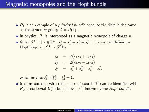
More on sections

Vector bundles always have at least one section, the null section s0with

φ−1i (s0(p)) = (p, 0)

in any local trivialization.

A principal bundle E only admits a global section if it is trivial:E = M × F .

A section in a principal bundle can be used to construct thetrivialization of the bundle which uses that we can define a rightaction which is independent of the local trivialization:

ua = φ(p, gia), a ∈ G


Associated Vector bundle

Given a principal fibre bundle P(M,G , π) and a k-dimensionalvector space V , and let ρ be a k dimensional representation of Gthen the associated vector bundle E = P ×ρ V is defined byidentifying the points

(u, v) and (ug , ρ(g)−1v) ∈ P × V

where u ∈ P, g ∈ G , and v ∈ V .

The projection πE : E → M is defined by πE (u, v) = π(u), which iswell defined because

πE (ug , ρ(g)−1v) = π(ug) = π(u) = πE (u, v)

The transition functions of E are given by ρ(tij(p)) where tij(p) arethe transition functions of P.

Conversely, a vector bundle naturally induces a principal bundleassociated with it.


Metric

Manifolds can carry further structure, for example a metric.

A metric g is a (0, 2) tensor which satisfies at each point p ∈ M :1 gp(U,V ) = gp(V ,U)2 gp(U,U) ≥ 0, with equality only when U = 0.

where U,V ∈ TpM.

The metric g provides an inner product for each tangent space TpM.

Notation:g = gµνdxµdxν .

If M is a submanifold of N with metric gN and f : M → N is theembedding map, then the induced metric gM is

gMµν(x) = gNαβ(f (x))∂f α

∂xµ∂f β

∂xν.


Connection for the Tangent bundle

Consider the “derivative” of a vector field V = V µ ∂∂xµ w.r.t. xν :

∂V µ

∂xν= lim4x→0

V µ(. . . , xν +4xν , . . . )− V µ(. . . , xν , . . . )

4xν

This doesn’t work as the first vector is defined at x +4x and thesecond at x .

We need to transport the vector V µ from x to x +4x “withoutchange”. This is known as parallel transport.

This is achieved by specifying a connection Γµνλ, namely the paralleltransported vector V µ is given by

V µ(x +4x) = V µ(x)− V λ(x)Γµνλ(x)4xν .

The covariant derivative of V w.r.t. xν is

lim4xν→0

V µ(x +4x)− V µ(x +4x)

4xν=∂V µ

∂xν+ V λΓµνλ.


The Levi-Civita Connection

We demand that the metric g is covariantly constant.

This means, if two vectors X and Y are parallel transported alongany curve, then the inner product g(X ,Y ) remains constant.

The condition∇V (g(X ,Y )) = 0,

gives us the Levi-Civita connection.

The Levi-Civita connection can be written as

Γκµν = 12gκλ (∂µgνλ + ∂νgµλ − ∂λgµν) .


General Relativity

The Levi-Civita connection doesn’t transform like a tensor. However,from it, we can build the curvature tensor:

Rκλµν = ∂µΓκνλ − ∂νΓκµλ + ΓηνλΓκµη − ΓηµλΓκνη.

Important contractions of the curvature tensor are the Ricci tensorRic :

Ricµν = Rλµλν .

and the scalar curvature R :

R = gµνRicµν .

Now, we have the ingredients for Einstein’s Equations of GeneralRelativity, namely

Ricµν − 12gµνR = 8πGTµν ,

where G is the gravitational constant and Tµν is the energymomentum tensor which describes the distribution of matter.


Yang-Mills theory

An example of Yang-Mills theory is given by the followingLagrangian density,

L =1

8Tr (FµνFµν) +

1

2(DµΦ)† DµΦ− U(Φ†Φ). (2)

where

DµΦ = ∂µΦ + AµΦ and Fµν = ∂µAν − ∂νAµ + [Aµ,Aν ] .

Here Φ is a two component complex scalar field.

Aµ is called a gauge field and is su(2)-valued, i.e. Aµ areanti-hermitian 2× 2 matrices.

Fµν is known as the field strength (also su(2)-valued)

This Lagrangian is Lorentz invariant.


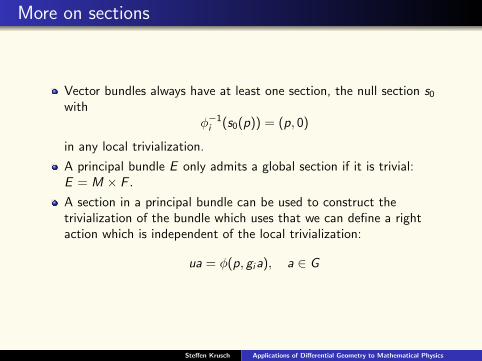
Gauge invariance

Lagrangian (2) is also invariant under local gauge transformations:

Let g ∈ SU(2) be a space-time dependent gauge transformation with

Φ 7→ gΦ, and Aµ 7→ gAµg−1 − ∂µgg−1.

The covariant derivative DµΦ transforms as

DµΦ 7→ ∂µ(gΦ) +(gAµg−1 − ∂µgg−1

)gΦ

= gDµΦ

Hence Φ†Φ 7→ (gΦ)†gΦ = Φ†g†gΦ = Φ†Φ, and similarly for

(DµΦ)† DµΦ.

Finally, Fµν 7→ gFµνg−1, so

Tr (FµνFµν)

is also invariant


Yang-Mills theory and Fibre bundles

In a more mathematical language:

The gauge field Aµ corresponds to the connection of the principalSU(2) bundle.

The field strength Fµν corresponds to the curvature of the principalSU(2) bundle.

The complex scalar field Φ is a section of the associated C2 vectorbundle.

The action of g ∈ SU(2) on Φ and Aµ is precisely what we expectfor an associated fibre bundle.

Surprisingly, mathematicians and physicist derived the same resultvery much independently!


Documents

Applications of Differential Geometry to Mathematical Physics · Ste en Krusch Applications of Di erential Geometry to Mathematical Physics. More on sections Vector bundles always