Applications of Computer Algebra to the Theory ofHypergeometric Series

A Dissertation

Presented to

The Faculty of the Graduate School of Arts and Sciences

Brandeis University

Department of Mathematics

Professor Ira Gessel, Advisor

In Partial Fulfillment

of the Requirements for the Degree

Doctor of Philosophy

by

Ping Zhou

May, 2003

This dissertation, directed and approved by Ping Zhou’s Committee, hasbeen accepted and approved by the Faculty of Brandeis University in partialfulfillment of the requirements for the degree of :

DOCTOR OF PHILOSOPHY

Dean of Arts and Sciences

Dissertation Committee:

Ira Gessel, Mathematics

Susan Parker, Mathematics

Martin Cohn, Computer Science, Brandeis University

Acknowledgements

I would like to express my deepest gratitude to Ira Gessel, my advisor, forhis mathematical insight and his guidance, and for the tremendous patiencehe has shown me and the enormous amount of time he has shared with meso generously. Without his help, I do not think I could even come close tofinishing this work.

I thank my family for always being there for me and would like to dedi-cate this thesis to my parents.

iii

ABSTRACT

Applications of Computer Algebra to the Theory ofHypergeometric Series

A dissertation presented to the faculty ofthe Graduate School of Arts and Sciences ofBrandeis University, Waltham, Massachusetts

by Ping Zhou

This thesis consists of two parts which both deal with the application of com-puters to the theory of hypergeometric series. In the first part of this thesiswe study how symbolic computational software, like Maple, can be used togenerate hypergeometric transformations systematically. Based on the ob-servation that

∑i

(∑j aij

)=

∑j

(∑i aij

), we generate double sums which

both inner sums can be evaluated by known hypergeometric summation the-orems. In a similar way, we generate transformations for two-variable hyper-geometric series. In the second part we focus on the WZ(Wilf-Zeilberger)method. We use a WZ pair to assign weight to a step and derive the pathindependence theorem which states that sum of the weights along pathsdepend only on the endpoints. We derive the change of variable theorem.Then we give some applications of path independence theorem. We alsoextend the WZ method to Euler’s and Pfaff’s transformations. We general-ized the application of the path independence theorem from hypergeometricfunctions to symmetric functions in the end.

iv

Contents

Chapter 0. Introduction 1

Chapter 1. Hypergeometric Transformations from Double Summation

1.1 Introduction 2

1.2 Deriving hypergeometric series by double summation 4

1.3 Generation of hypergeometric transformation via Maple 7

1.4 Transformations Generated by the Maple Program 13

1.5 More Hypergeometric Transformations via Index Shifting 18

1.6 Transformations Generated by the Maple Program via Index shifting 19

Chapter 2. Hypergeometric Transformations of Two Variables by Coefficient Extraction

2.1 A Transformation of Appell’s F1 21

2.2 A Systematic Way to Generate Transformations 22

2.3 From Gauss’s and Gauss’s Theorem 24

2.4 From Gauss’s and Saalschutz’s Theorems 26

2.6 Identification of the Transformations 26

2.7 Trivial Transformations 27

2.8 Description of the Program 29

Chapter 3. WZ Forms and their Change of Variables Theorem

3.1 Introduction to WZ Forms 31

3.2 Path Independence Theorem and Change of Variables Theorem for WZ Forms 32

3.3 Examples of Path Independence Theorem 34

3.4 WZ Forms of Linear Hypergeometric Transformations 38

3.5 Symmetric Functions and Path Independence Theorem of WZ Forms 45

v

Chapter 0. Introduction

In chapter 1 we look at double sums of the form

∑i,j

(a1)p1i+q1j · · · (an)pni+qnj

i!j!c1

ic2j .

We associate such a double sum with a multiset {(p1, q1), · · · (pn, qn)}, which we call the partition

associated with the sum. We study the use of Maple to generate all the partitions whose correspond-

ing double sums can be evaluated when first summed on i and when first summed on j. This gives

us transformations for hypergeometric series. In chapter 2, we start with a hypergeometric series

with two variables, say f(x, y) =∑

aijxiyj , then we do a simple transformation on the variables,

like (1 − x)p(1 − y)qf( x1−x , y

1−y ) and express the coefficient of xiyj as hypergeometric series. We

then evaluate the hypergeometric series by known hypergeometric summation theorems and obtain

a hypergeometric transformations in two variables.

In chapter 3, we study WZ forms for hypergeometric series. In particular, we derive the path

independence theorem for WZ forms and give some applications of the path independence theorem.

We prove the change of variables theorem for WZ forms which is a straightforward consequence of

the path independence theorem. We show how the change of variables theorem gives the connection

between various forms of a hypergeometric evaluation and its WZ forms. We also extend the WZ

method to Euler’s and Pfaff’s transformations. In the end of chapter 3, we generalize the application

of the path independence theorem from hypergeometric functions to symmetric functions.

1

Chapter 1. Hypergeometric Transformations from Double Summation

§1.1 Introduction

A hypergeometric series∑

i≥0 ai is a series in which the ratio of every two consecutive terms,ai+1

ai, is a rational function of the summation index i. If we define a rising factorial in a to be

(a)n =

a(a + 1) · · · (a + n− 1), if n > 0;

(−1)n

(1− a)−n, if n < 0;

1, if n = 0

then obviously, the following is a hypergeometric series

∞∑i=0

(a1)i · · · (an)i

i!(b1)i · · · (bm)ivi, (1.1.1)

and we denote it by

nFm

(a1, · · · , an

b1, · · · , bm

∣∣∣∣ v) . (1.1.2)

We call a1, · · · , an its numerator parameters, b1, · · · , bm its denominator parameters, and z its argu-

ment. Note that

(a)n =Γ(a + n)

Γ(a)

as long as a is not a negative integer. There are some well-known hypergeometric identities such as

the binomial theorem

1F0

(a

−

∣∣∣∣x) = (1− x)−a,

Gauss’s theorem

2F1

(a, b

c

∣∣∣∣ 1) =Γ(c)Γ(c− a− b)Γ(c− a)Γ(c− b)

,

where R(c− a− b) > 0, or a or b is a nonpositive integer and Saalschutz’s theorem

3F2

(a, b,−n

c, d

∣∣∣∣ 1) =(c− a)n(c− b)n

(c)n(c− a− b)n,

where a+b−n+1 = c+d, and n is a nonnegative integer. In Saalschutz’s theorem the hypergeometric

series is said to be balanced since its parameters satisfy the relation a + b− n + 1 = c + d [3, (2.5)].

An identity which transforms one hypergeometric series to another one is called a hypergeometric

transformation. There are many ways to get hypergeometric transformations. One of the most

powerful techniques is based on the observation that

∑i

(∑j

aij

)=∑

j

(∑i

aij

).

2

This technique has been used widely in the theory of hypergeometric series and various authors

have studied this method somewhat systematically [3, 4], but have restricted their attention to what

appeared to be the most promising cases, because looking at all possible cases would be too tedious.

However, the computer, more specifically the mathematical symbolic computation software such as

Maple, makes it possible for us to consider all possibilities. It can help generate all possible double

sums, examine each one of them and evaluate it if possible. For example, we can come up with a

Maple program to systematically apply the method of double summation in the cases in which one

side is evaluated by Gauss’s, the binomial or Saalschutz’s theorem and the other side is evaluated

by one of these theorems as well.

3

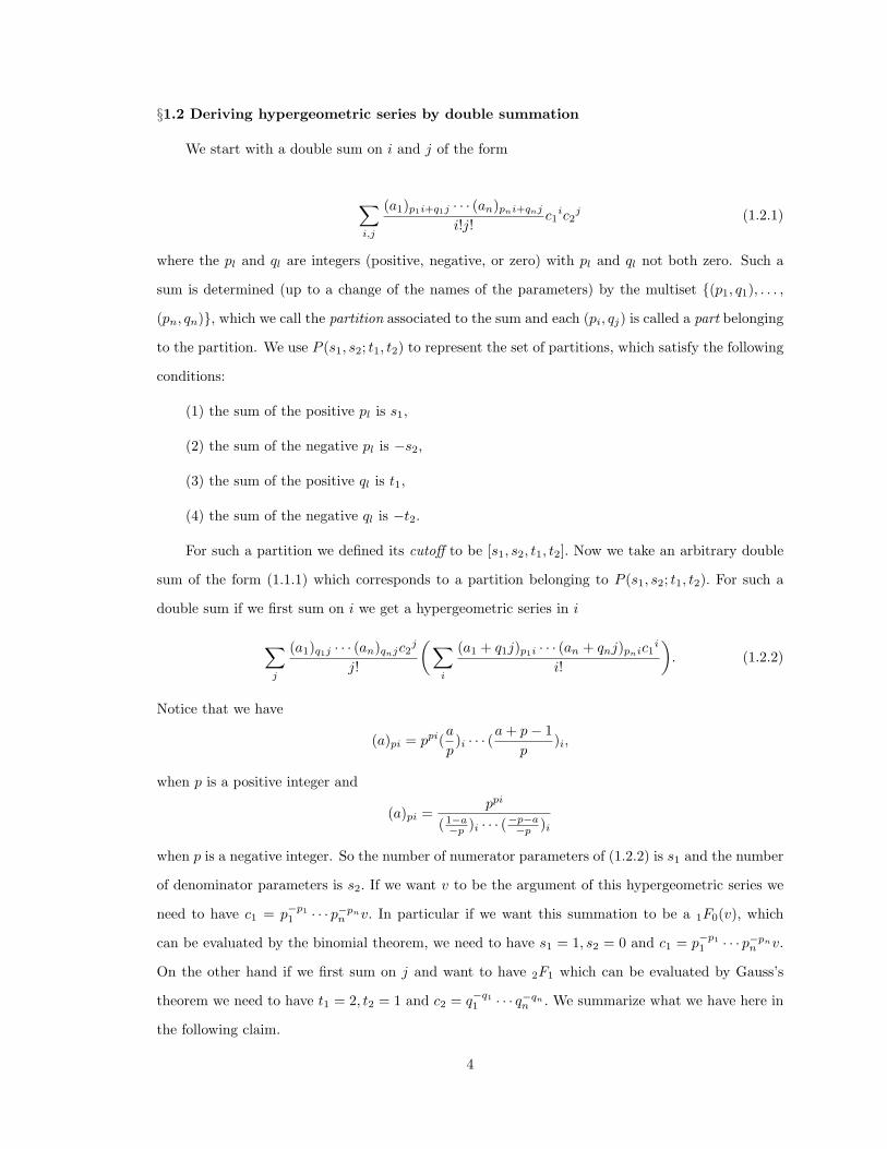
§1.2 Deriving hypergeometric series by double summation

We start with a double sum on i and j of the form

∑i,j

(a1)p1i+q1j · · · (an)pni+qnj

i!j!c1

ic2j (1.2.1)

where the pl and ql are integers (positive, negative, or zero) with pl and ql not both zero. Such a

sum is determined (up to a change of the names of the parameters) by the multiset {(p1, q1), . . . ,

(pn, qn)}, which we call the partition associated to the sum and each (pi, qj) is called a part belonging

to the partition. We use P (s1, s2; t1, t2) to represent the set of partitions, which satisfy the following

conditions:

(1) the sum of the positive pl is s1,

(2) the sum of the negative pl is −s2,

(3) the sum of the positive ql is t1,

(4) the sum of the negative ql is −t2.

For such a partition we defined its cutoff to be [s1, s2, t1, t2]. Now we take an arbitrary double

sum of the form (1.1.1) which corresponds to a partition belonging to P (s1, s2; t1, t2). For such a

double sum if we first sum on i we get a hypergeometric series in i

∑j

(a1)q1j · · · (an)qnjc2j

j!

(∑i

(a1 + q1j)p1i · · · (an + qnj)pnic1i

i!

). (1.2.2)

Notice that we have

(a)pi = ppi(a

p)i · · · (

a + p− 1p

)i,

when p is a positive integer and

(a)pi =ppi

( 1−a−p )i · · · (−p−a

−p )i

when p is a negative integer. So the number of numerator parameters of (1.2.2) is s1 and the number

of denominator parameters is s2. If we want v to be the argument of this hypergeometric series we

need to have c1 = p−p11 · · · p−pn

n v. In particular if we want this summation to be a 1F0(v), which

can be evaluated by the binomial theorem, we need to have s1 = 1, s2 = 0 and c1 = p−p11 · · · p−pn

n v.

On the other hand if we first sum on j and want to have 2F1 which can be evaluated by Gauss’s

theorem we need to have t1 = 2, t2 = 1 and c2 = q−q11 · · · q−qn

n . We summarize what we have here in

the following claim.

4

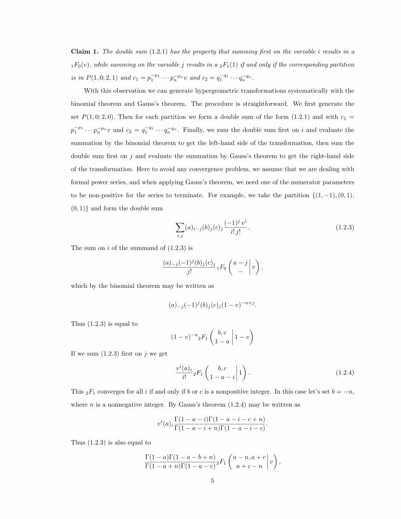
Claim 1. The double sum (1.2.1) has the property that summing first on the variable i results in a

1F0(v), while summing on the variable j results in a 2F1(1) if and only if the corresponding partition

is in P (1, 0; 2, 1) and c1 = p−p11 · · · p−pn

n v and c2 = q−q11 · · · q−qn

n .

With this observation we can generate hypergeometric transformations systematically with the

binomial theorem and Gauss’s theorem. The procedure is straightforward. We first generate the

set P (1, 0; 2, 0). Then for each partition we form a double sum of the form (1.2.1) and with c1 =

p−p11 · · · p−pn

n v and c2 = q−q11 · · · q−qn

n . Finally, we sum the double sum first on i and evaluate the

summation by the binomial theorem to get the left-hand side of the transformation, then sum the

double sum first on j and evaluate the summation by Gauss’s theorem to get the right-hand side

of the transformation. Here to avoid any convergence problem, we assume that we are dealing with

formal power series, and when applying Gauss’s theorem, we need one of the numerator parameters

to be non-positive for the series to terminate. For example, we take the partition {(1,−1), (0, 1),

(0, 1)} and form the double sum

∑i,j

(a)i−j(b)j(c)j(−1)j vi

i! j!. (1.2.3)

The sum on i of the summand of (1.2.3) is

(a)−j(−1)j(b)j(c)j

j! 1F0

(a− j

−

∣∣∣∣ v) ,

which by the binomial theorem may be written as

(a)−j(−1)j(b)j(c)j(1− v)−a+j .

Thus (1.2.3) is equal to

(1− v)−a2F1

(b, c

1− a

∣∣∣∣ 1− v

)If we sum (1.2.3) first on j we get

vi(a)i

i! 2F1

(b, c

1− a− i

∣∣∣∣ 1) . (1.2.4)

This 2F1 converges for all i if and only if b or c is a nonpositive integer. In this case let’s set b = −n,

where n is a nonnegative integer. By Gauss’s theorem (1.2.4) may be written as

vi(a)iΓ(1− a− i)Γ(1− a− i− c + n)Γ(1− a− i + n)Γ(1− a− i− c)

.

Thus (1.2.3) is also equal to

Γ(1− a)Γ(1− a− b + n)Γ(1− a + n)Γ(1− a− c) 2F1

(a− n, a + c

a + c− n

∣∣∣∣ v) ,

5

and we get a well known linear transformation

(1− v)−a2F1

(−n, c

1− a

∣∣∣∣ 1− v

)=

Γ(1− a)Γ(1− a− c + n)Γ(1− a + n)Γ(1− a− c) 2F1

(a− n, a + c

a + c− n

∣∣∣∣ v)=

(1− a− c)n

(1− a)n2F1

(a− n, a + c

a + c− n

∣∣∣∣ v) .

6

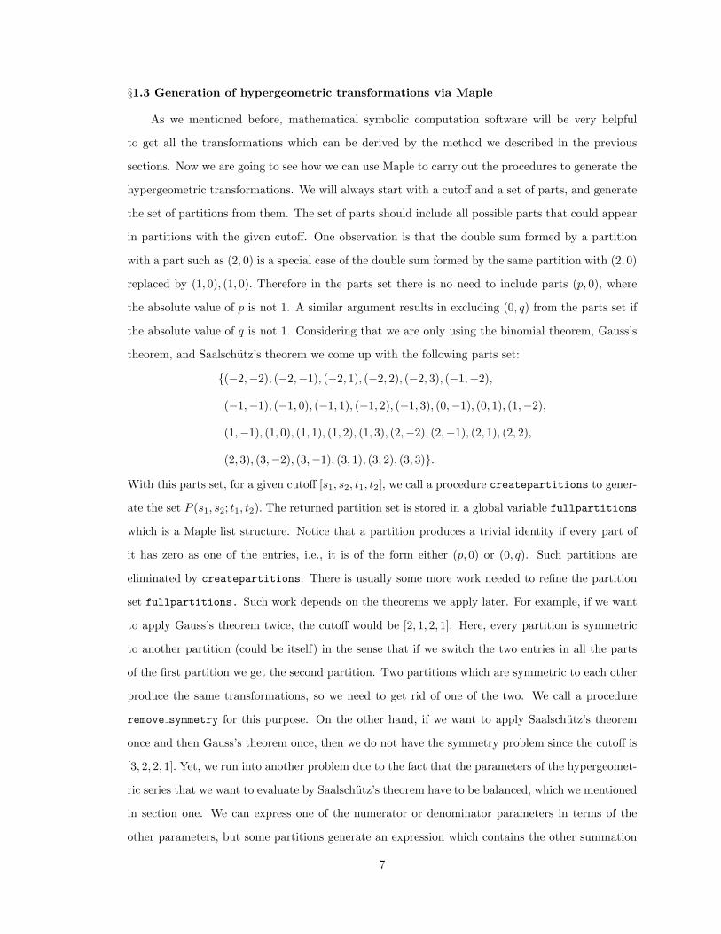
§1.3 Generation of hypergeometric transformations via Maple

As we mentioned before, mathematical symbolic computation software will be very helpful

to get all the transformations which can be derived by the method we described in the previous

sections. Now we are going to see how we can use Maple to carry out the procedures to generate the

hypergeometric transformations. We will always start with a cutoff and a set of parts, and generate

the set of partitions from them. The set of parts should include all possible parts that could appear

in partitions with the given cutoff. One observation is that the double sum formed by a partition

with a part such as (2, 0) is a special case of the double sum formed by the same partition with (2, 0)

replaced by (1, 0), (1, 0). Therefore in the parts set there is no need to include parts (p, 0), where

the absolute value of p is not 1. A similar argument results in excluding (0, q) from the parts set if

the absolute value of q is not 1. Considering that we are only using the binomial theorem, Gauss’s

theorem, and Saalschutz’s theorem we come up with the following parts set:

{(−2,−2), (−2,−1), (−2, 1), (−2, 2), (−2, 3), (−1,−2),

(−1,−1), (−1, 0), (−1, 1), (−1, 2), (−1, 3), (0,−1), (0, 1), (1,−2),

(1,−1), (1, 0), (1, 1), (1, 2), (1, 3), (2,−2), (2,−1), (2, 1), (2, 2),

(2, 3), (3,−2), (3,−1), (3, 1), (3, 2), (3, 3)}.

With this parts set, for a given cutoff [s1, s2, t1, t2], we call a procedure createpartitions to gener-

ate the set P (s1, s2; t1, t2). The returned partition set is stored in a global variable fullpartitions

which is a Maple list structure. Notice that a partition produces a trivial identity if every part of

it has zero as one of the entries, i.e., it is of the form either (p, 0) or (0, q). Such partitions are

eliminated by createpartitions. There is usually some more work needed to refine the partition

set fullpartitions. Such work depends on the theorems we apply later. For example, if we want

to apply Gauss’s theorem twice, the cutoff would be [2, 1, 2, 1]. Here, every partition is symmetric

to another partition (could be itself) in the sense that if we switch the two entries in all the parts

of the first partition we get the second partition. Two partitions which are symmetric to each other

produce the same transformations, so we need to get rid of one of the two. We call a procedure

remove symmetry for this purpose. On the other hand, if we want to apply Saalschutz’s theorem

once and then Gauss’s theorem once, then we do not have the symmetry problem since the cutoff is

[3, 2, 2, 1]. Yet, we run into another problem due to the fact that the parameters of the hypergeomet-

ric series that we want to evaluate by Saalschutz’s theorem have to be balanced, which we mentioned

in section one. We can express one of the numerator or denominator parameters in terms of the

other parameters, but some partitions generate an expression which contains the other summation

7

index. For example, partition ((−1, 2), (1,−1), (1, 0), (1, 0), (−1, 0)) has cutoff [3, 2, 2, 1]. We form a

double sum of the form (1.2.1) from this partition and first sum on i we get

(a)−i+2 j(b)i−j(c)i(d)i(e)−i(−1)2i+j(2)−2j

i! j!.

If we first sum this sum on i we get

∑j

(a)2 j

(14

)j (b)−j (−1)j

j! 3F2

(b− j, c, d

1− a− 2 j, 1− e

∣∣∣∣1) .

In order to use Saalschutz’s theorem the parameters of 3F2 needs to satisfy the condition

b− j + c + d + 1 = 1− a− 2j + 1− e.

Since condition is dependent on j it cannot produce a valid variable substitution expression. If the

coefficient of j on the left hand side of the equation is equal to the coeffient of j on the right hand

side, then we can get a variable substition expression independent of j. In fact the coefficient on

the left hand side is the sum of the second tuple for all parts whose first tuple is positive, while

the coefficient on the right hand side is the negative of the sum of the second tuple for all parts

whose first tuple is negative. In general, a partition P from P (3, 2; 2, 1) produces a valid substitution

expression if and only if the terms containing the summation index cancel each other, i.e.:∑(p,q)∈P,p>0

q =∑

(p,q)∈P,p<0

(−q).

We call a procedure select balanced to just include such good partitions in the fullpartitions

list. The following is the Maple output when calling some of the procedures we just described.

> cutoff := [2, 1, 2, 1]

> createpartitions(cutoff);

> nops(fullpartitions);

24

> remove symmetry();

[[[−1, 2], [0, −1], [1, 0], [1, 0]], [[−1, −1], [0, 1], [0, 1], [1, 0], [1, 0]],

[[−1, 1], [0, −1], [0, 1], [1, 0], [1, 0]], [[−1, 2], [1, −1], [1, 0]], [[−1, 1], [0, 1], [1, −1], [1, 0]],

[[−1, −1], [1, 1], [1, 1]], [[−1, 0], [0, −1], [1, 1], [1, 1]], [[−1, 1], [1, −1], [1, 1]],

[[−1, 0], [0, 1], [1, −1], [1, 1]], [[−1, −1], [0, 1], [1, 0], [1, 1]],

[[−1, 0], [0, −1], [0, 1], [1, 0], [1, 1]], [[−1, 0], [1, −1], [1, 2]], [[−1, −1], [1, 0], [1, 2]],

[[−1, 0], [0, −1], [1, 0], [1, 2]], [[−1, 2], [2, −1]], [[−1, −1], [2, 2]], [[−1, 0], [0, −1], [2, 2]]]

8

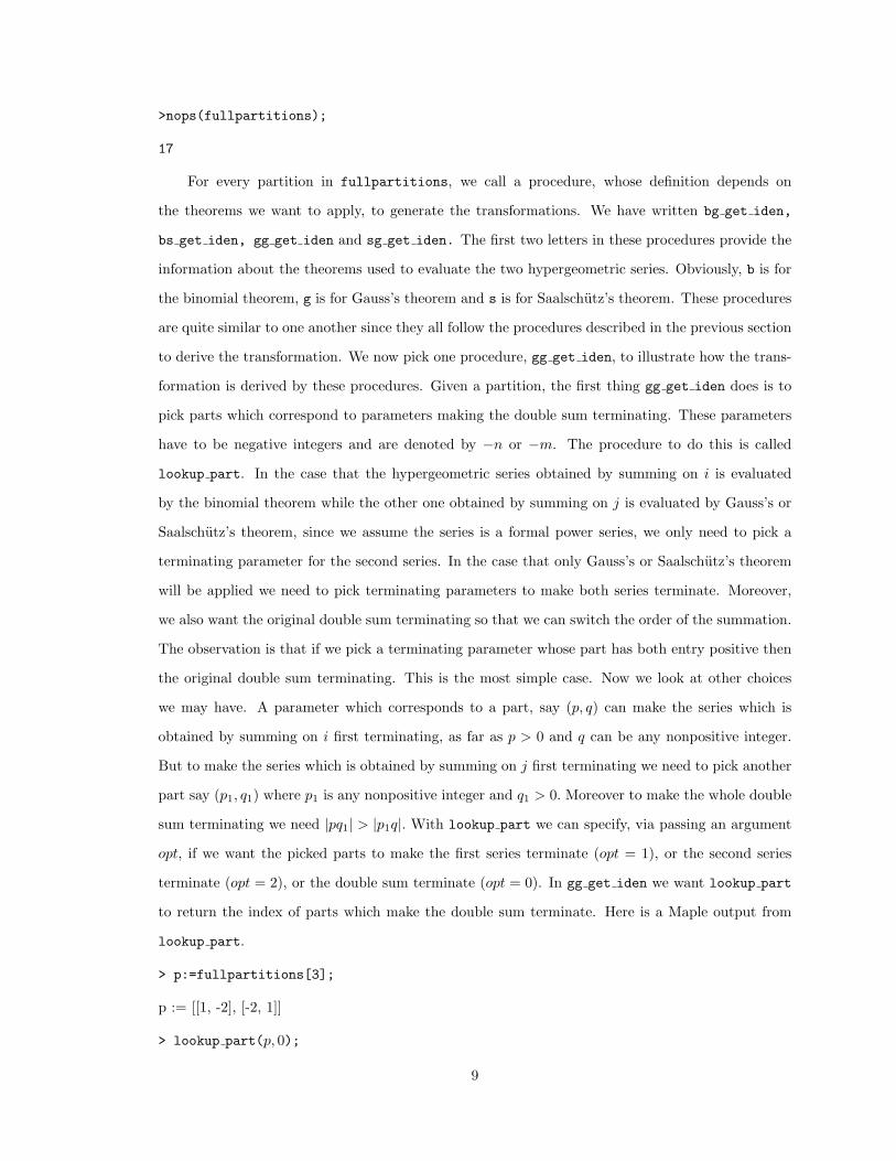
>nops(fullpartitions);

17

For every partition in fullpartitions, we call a procedure, whose definition depends on

the theorems we want to apply, to generate the transformations. We have written bg get iden,

bs get iden, gg get iden and sg get iden. The first two letters in these procedures provide the

information about the theorems used to evaluate the two hypergeometric series. Obviously, b is for

the binomial theorem, g is for Gauss’s theorem and s is for Saalschutz’s theorem. These procedures

are quite similar to one another since they all follow the procedures described in the previous section

to derive the transformation. We now pick one procedure, gg get iden, to illustrate how the trans-

formation is derived by these procedures. Given a partition, the first thing gg get iden does is to

pick parts which correspond to parameters making the double sum terminating. These parameters

have to be negative integers and are denoted by −n or −m. The procedure to do this is called

lookup part. In the case that the hypergeometric series obtained by summing on i is evaluated

by the binomial theorem while the other one obtained by summing on j is evaluated by Gauss’s or

Saalschutz’s theorem, since we assume the series is a formal power series, we only need to pick a

terminating parameter for the second series. In the case that only Gauss’s or Saalschutz’s theorem

will be applied we need to pick terminating parameters to make both series terminate. Moreover,

we also want the original double sum terminating so that we can switch the order of the summation.

The observation is that if we pick a terminating parameter whose part has both entry positive then

the original double sum terminating. This is the most simple case. Now we look at other choices

we may have. A parameter which corresponds to a part, say (p, q) can make the series which is

obtained by summing on i first terminating, as far as p > 0 and q can be any nonpositive integer.

But to make the series which is obtained by summing on j first terminating we need to pick another

part say (p1, q1) where p1 is any nonpositive integer and q1 > 0. Moreover to make the whole double

sum terminating we need |pq1| > |p1q|. With lookup part we can specify, via passing an argument

opt, if we want the picked parts to make the first series terminate (opt = 1), or the second series

terminate (opt = 2), or the double sum terminate (opt = 0). In gg get iden we want lookup part

to return the index of parts which make the double sum terminate. Here is a Maple output from

lookup part.

> p:=fullpartitions[3];

p := [[1, -2], [-2, 1]]

> lookup part(p, 0);

9

[]

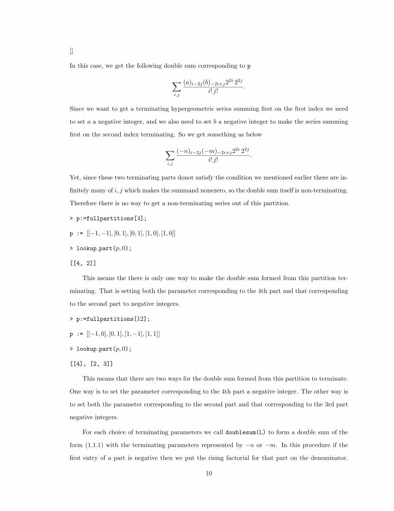
In this case, we get the following double sum corresponding to p

∑i,j

(a)i−2j(b)−2i+j22i 22j

i! j!.

Since we want to get a terminating hypergeometric series summing first on the first index we need

to set a a negative integer, and we also need to set b a negative integer to make the series summing

first on the second index terminating. So we get something as below

∑i,j

(−n)i−2j(−m)−2i+j22i 22j

i! j!.

Yet, since these two terminating parts donot satisfy the condition we mentioned earlier there are in-

finitely many of i, j which makes the summand nonezero, so the double sum itself is non-terminating.

Therefore there is no way to get a non-terminating series out of this partition.

> p:=fullpartitions[4];

p := [[−1,−1], [0, 1], [0, 1], [1, 0], [1, 0]]

> lookup part(p, 0);

[[4, 2]]

This means the there is only one way to make the double sum formed from this partition ter-

minating. That is setting both the parameter corresponding to the 4th part and that corresponding

to the second part to negative integers.

> p:=fullpartitions[12];

p := [[−1, 0], [0, 1], [1,−1], [1, 1]]

> lookup part(p, 0);

[[4], [2, 3]]

This means that there are two ways for the double sum formed from this partition to terminate.

One way is to set the parameter corresponding to the 4th part a negative integer. The other way is

to set both the parameter corresponding to the second part and that corresponding to the 3rd part

negative integers.

For each choice of terminating parameters we call doublesum(L) to form a double sum of the

form (1.1.1) with the terminating parameters represented by −n or −m. In this procedure if the

first entry of a part is negative then we put the rising factorial for that part on the denominator.

10

We then call toF(summand, i) to convert hypergeometric series obtained by i into the form defined

by (1.1.2) and procedure gauss evaluates this hypergeometric series by Gauss’s theorem. We use

hypercombine to convert the summand to rising factorials in j and combine factorials in fractional j,

if such factorials exist, to one factorial in j if possible. In the end tor is called to convert the summand

to be a product of rising factorials in n or m. In this way, we obtain one side of the transformation

and the other side is obtained in a similar manner.

The following shows how all the procedures can be used to generate transformations from a

partition. Note that " in Maple denotes the result of the last calculation.

> var:=[a,b,c,d,e,f,g,h];

> part:=[[−1, 0], [0, 1], [1,−1], [1, 1]]:

> lookup part(",0);

[[4], [2, 3]]

> doublesum(part);

(−1)j(b)j(c)i−j(d)i+j

i! j! (a)i

> d sum:=subs(var[4]=-n, ");

d sum :=(−1)j(b)j(c)i−j(−n)i+j

i! j! (a)i

> L0:=toF(d sum, j);

L0 :=(c)i(−n)iF ([b,−n + i], [1− c− i], 1)

i!(a)i

> L1:=gauss(L0);

L1 :=(c)i(−n)iΓ(1− c− i)Γ(1− c− 2i− b + n)

i!(a)iΓ(1− c− i− b)Γ(1− c− 2i + n)

> L2:=toF(L1,i):

> L3:=tor(",n);

L3 :=(1− c− b)n

(1− c)nF ([−n, c + b,

12c− 1

2n,

12c− 1

2n +

12], [a,

12c +

12b− 1

2n,

12c +

12b− 1

2n +

12], 1)

> R0:=toF(d sum,i);

R0 :=(−1)j(b)j(c)−j(−n)j

j!F ([c− j,−n + j], [a], 1)

> gauss(");

(−1)j(b)j(c)−j(−n)jΓ(a)Γ(a− c + n)j!Γ(a− c + j)Γ(a + n− j)

11

> toF(",j);

Γ(a)Γ(a− c + n)Γ(a− c)Γ(a + n)

F ([b,−n, 1− a− n], [1− c, a− c],−1)

> tor(",n);

(a− c)n

(a)nF ([b,−n, 1− a− n], [1− c, a− c],−1)

So the hypergeometric transformation we got here is

{(−1, 0), (0, 1), (1,−1), (1, 1)}

(1− c− b)n

(1− c)n4F3

(−n, c + b, c

2 −n2 , c

2 −n2 + 1

2

a, c2 + b

2 −n2 , c

2 + b2 −

n2 + 1

2

∣∣∣∣1)

=(a− c)n

(a)n3F2

(b,−n, 1− a− n

1− c, a− c

∣∣∣∣− 1)

. (1.3.1)

The hypergeometric transformation we get in the same way from setting the second and third

parameters nonpositive is

{(−1, 0), (0, 1), (1,−1), (1, 1)}

(1 + m− d)n

(1 + m)n4F3

(d,−m− n,−m

2 + d2 ,−m

2 + d2 + 1

2

1− a,−m2 − n

2 + d2 ,−m

2 − n2 + d

2 + 12

∣∣∣∣1)

=(1− a− d)m

(1− a)m3F2

(−n, d, a + d

1 + m, 1− a + m

∣∣∣∣− 1)

(1.3.2)

12

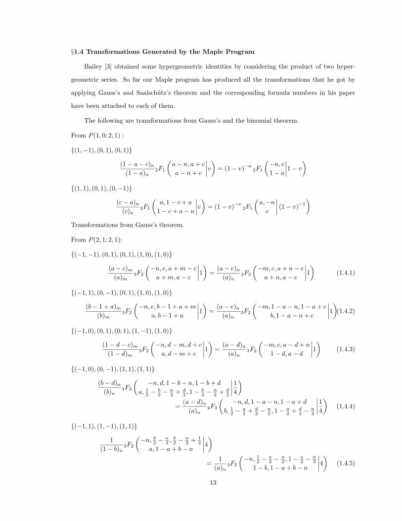
§1.4 Transformations Generated by the Maple Program

Bailey [3] obtained some hypergeometric identities by considering the product of two hyper-

geometric series. So far our Maple program has produced all the transformations that he got by

applying Gauss’s and Saalschutz’s theorem and the corresponding formula numbers in his paper

have been attached to each of them.

The following are transformations from Gauss’s and the binomial theorem.

From P (1, 0; 2, 1) :

{(1,−1), (0, 1), (0, 1)}

(1− a− c)n

(1− a)n2F1

(a− n, a + c

a− n + c

∣∣∣∣v) = (1− v)−a2F1

(−n, c

1− a

∣∣∣∣1− v

){(1, 1), (0, 1), (0,−1)}

(c− a)n

(c)n2F1

(a, 1− c + a

1− c + a− n

∣∣∣∣v) = (1− v)−a2F1

(a,−n

c

∣∣∣∣ (1− v)−1

)Transformations from Gauss’s theorem.

From P (2, 1; 2, 1):

{(−1,−1), (0, 1), (0, 1), (1, 0), (1, 0)}

(a− c)m

(a)m3F2

(−n, e, a + m− c

a + m,a− c

∣∣∣∣1) =(a− e)n

(a)n3F2

(−m, c, a + n− e

a + n, a− e

∣∣∣∣1) (1.4.1)

{(−1, 1), (0,−1), (0, 1), (1, 0), (1, 0)}

(b− 1 + a)m

(b)m3F2

(−n, e, b− 1 + a + m

a, b− 1 + a

∣∣∣∣1) =(a− e)n

(a)n3F2

(−m, 1− a− n, 1− a + e

b, 1− a− n + e

∣∣∣∣1)(1.4.2)

{(−1, 0), (0, 1), (0, 1), (1,−1), (1, 0)}

(1− d− c)m

(1− d)m3F2

(−n, d−m, d + c

a, d−m + c

∣∣∣∣1) =(a− d)n

(a)n3F2

(−m, c, a− d + n

1− d, a− d

∣∣∣∣1) (1.4.3)

{(−1, 0), (0,−1), (1, 1), (1, 1)}

(b− d)n

(b)n4F3

(−n, d, 1− b− n, 1− b + d

a, 12 −

b2 −

n2 + d

2 , 1− b2 −

n2 + d

2

∣∣∣∣14)

=(a− d)n

(a)n4F3

(−n, d, 1− a− n, 1− a + d

b, 12 −

a2 + d

2 −n2 , 1− a

2 + d2 −

n2

∣∣∣∣14)

(1.4.4)

{(−1, 1), (1,−1), (1, 1)}

1(1− b)n

3F2

(−n, b

2 −n2 , b

2 −n2 + 1

2

a, 1− a + b− n

∣∣∣∣4)=

1(a)n

3F2

(−n, 1

2 −a2 −

n2 , 1− a

2 −n2

1− b, 1− a + b− n

∣∣∣∣4) (1.4.5)

13

{(−1, 0), (0, 1), (1,−1), (1, 1)}

(1− c− b)n

(1− c)n4F3

(−n, c + b, c

2 −n2 , c

2 −n2 + 1

2

a, c2 + b

2 −n2 , c

2 + b2 −

n2 + 1

2

∣∣∣∣1)

=(a− c)n

(a)n3F2

(b,−n, 1− a− n

1− c, a− c

∣∣∣∣− 1)

(1.4.6)

{(−1, 1), (0,−1), (1, 0), (1, 1)}

(b− 1 + a)n

(b)n3F2

(c,−n, 1− b− n

a, b− 1 + a

∣∣∣∣− 1)

=(a− c)n

(a)n4F3

(−n, 1− a + c, 1

2 −a2 −

n2 , 1− a

2 −n2

b, 12 −

a2 + c

2 −n2 , 1− a

2 + c2 −

n2

∣∣∣∣1)

(1.4.7)

{(−1, 0), (0,−1), (0, 1), (1, 0), (1, 1)}

(b− c)n

(b)n3F2

(d,−n, 1− b− n

a, 1− b + c− n

∣∣∣∣1) =(a− d)n

(a)n3F2

(c,−n, 1− a− n

b, 1− a + d− n

∣∣∣∣1) (1.4.8)

{(−1, 0), (0,−1), (0, 1), (1, 0), (1, 1)}

(b− e)m

(b)m3F2

(−n, e, 1− b + e

a, 1− b−m + e

∣∣∣∣1) =(a− e)n

(a)n3F2

(−m, e, 1− a + e

b, 1− a− n + e

∣∣∣∣1) (1.4.9)

{(−1, 0), (1,−1), (1, 2)}

( 12 − b)n2n

(1− 2 b)n4F3

(−n, 2 b

3 − n3 , 2 b

3 − n3 + 1

3 , 2 b3 − n

3 + 23

a, 14 + b

2 −n2 , 3

4 + b2 −

n2

∣∣∣∣2732

)

=(a− b)n

(a)n4F3

(−n

2 ,−n2 + 1

2 , 12 −

a2 −

n2 , 1− a

2 −n2

1− b, 1− a + b− n, a− b

∣∣∣∣− 4)

(1.4.10)

{(−1,−1), (1, 0), (1, 2)}

(a− 12 )n2n

(2 a− 1)n2F1

(b,−n

2 a + n− 1

∣∣∣∣2) =(a− b)n

(a)n3F2

(−n

2 ,−n2 + 1

2 , 1− a− n

1− a + b− n, a− b

∣∣∣∣1) (1.4.11)

{(−1, 0), (0,−1), (1, 0), (1, 2)}

(b− 12 )n2n

(2 b− 1)n3F2

(c,−n, 2− 2 b− n

a, 32 − b− n

∣∣∣∣12)

=(a− c)n

(a)n4F3

(−n

2 ,−n2 + 1

2 , 12 −

a2 −

n2 , 1− a

2 −n2

b, 12 −

a2 + c

2 −n2 , 1− a

2 + c2 −

n2

∣∣∣∣1)

(1.4.12)

{(−1, 1), (0,−1), (2, 1)}

(b− 1 + a)n

(b)n4F3

(−n

2 ,−n2 + 1

2 , 12 −

b2 −

n2 , 1− b

2 −n2

a, 2− b− a− n, b− 1 + a

∣∣∣∣− 4)

=(a− 1

2 )n2n

(2 a− 1)n4F3

(−n, 2

3 −2 a3 − n

3 , 1− 2 a3 − n

3 , 43 −

2 a3 − n

3

b, 34 −

a2 −

n2 , 5

4 −a2 −

n2

∣∣∣∣2732

)(1.4.13)

14

{(−1,−1), (0, 1), (2, 1)}

(a− b)n

(a)n3F2

(−n

2 ,−n2 + 1

2 , 1− a− n

1− a + b− n, a− b

∣∣∣∣1) =(a− 1

2 )n2n

(2 a− 1)n2F1

(b,−n

2 a + n− 1

∣∣∣∣2) (1.4.14)

{(−1, 0), (0,−1), (0, 1), (2, 1)}

(b− c)n

(b)n4F3

(−n

2 ,−n2 + 1

2 , 12 −

b2 −

n2 , 1− b

2 −n2

a, 12 −

b2 + c

2 −n2 , 1− b

2 + c2 −

n2

∣∣∣∣1)

=(a− 1

2 )n2n

(2 a− 1)n3F2

(c,−n, 2− 2 a− n

b, 32 − a− n

∣∣∣∣12)

(1.4.15)

{(−1, 0), (0,−1), (2, 2)}

(b− 12 )n

(2 b− 1)n4F3

(−n

2 ,−n2 + 1

2 , 1− b− n2 , 3

2 − b− n2

a, 34 −

b2 −

n2 , 5

4 −b2 −

n2

∣∣∣∣14)

=(a− 1

2 )n

(2 a− 1)n4F3

(−n

2 ,−n2 + 1

2 , 1− a− n2 , 3

2 − a− n2

b, 34 −

a2 −

n2 , 5

4 −a2 −

n2

∣∣∣∣14)

(1.4.16)

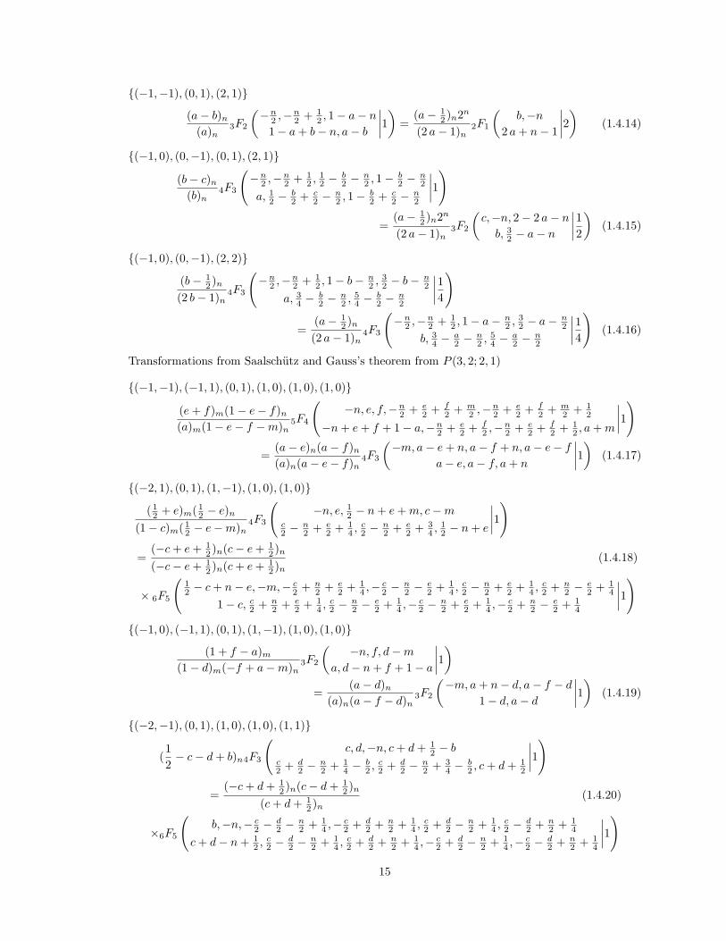
Transformations from Saalschutz and Gauss’s theorem from P (3, 2; 2, 1)

{(−1,−1), (−1, 1), (0, 1), (1, 0), (1, 0), (1, 0)}

(e + f)m(1− e− f)n

(a)m(1− e− f −m)n5F4

(−n, e, f,−n

2 + e2 + f

2 + m2 ,−n

2 + e2 + f

2 + m2 + 1

2

−n + e + f + 1− a,−n2 + e

2 + f2 ,−n

2 + e2 + f

2 + 12 , a + m

∣∣∣∣1)

=(a− e)n(a− f)n

(a)n(a− e− f)n4F3

(−m,a− e + n, a− f + n, a− e− f

a− e, a− f, a + n

∣∣∣∣1) (1.4.17)

{(−2, 1), (0, 1), (1,−1), (1, 0), (1, 0)}

( 12 + e)m( 1

2 − e)n

(1− c)m( 12 − e−m)n

4F3

(−n, e, 1

2 − n + e + m, c−mc2 −

n2 + e

2 + 14 , c

2 −n2 + e

2 + 34 , 1

2 − n + e

∣∣∣∣1)

=(−c + e + 1

2 )n(c− e + 12 )n

(−c− e + 12 )n(c + e + 1

2 )n

× 6F5

(12 − c + n− e,−m,− c

2 + n2 + e

2 + 14 ,− c

2 −n2 −

e2 + 1

4 , c2 −

n2 + e

2 + 14 , c

2 + n2 −

e2 + 1

4

1− c, c2 + n

2 + e2 + 1

4 , c2 −

n2 −

e2 + 1

4 ,− c2 −

n2 + e

2 + 14 ,− c

2 + n2 −

e2 + 1

4

∣∣∣∣1)(1.4.18)

{(−1, 0), (−1, 1), (0, 1), (1,−1), (1, 0), (1, 0)}

(1 + f − a)m

(1− d)m(−f + a−m)n3F2

(−n, f, d−m

a, d− n + f + 1− a

∣∣∣∣1)=

(a− d)n

(a)n(a− f − d)n3F2

(−m,a + n− d, a− f − d

1− d, a− d

∣∣∣∣1) (1.4.19)

{(−2,−1), (0, 1), (1, 0), (1, 0), (1, 1)}

(12− c− d + b)n4F3

(c, d,−n, c + d + 1

2 − bc2 + d

2 −n2 + 1

4 −b2 , c

2 + d2 −

n2 + 3

4 −b2 , c + d + 1

2

∣∣∣∣1)

=(−c + d + 1

2 )n(c− d + 12 )n

(c + d + 12 )n

×6F5

(b,−n,− c

2 −d2 −

n2 + 1

4 ,− c2 + d

2 + n2 + 1

4 , c2 + d

2 −n2 + 1

4 , c2 −

d2 + n

2 + 14

c + d− n + 12 , c

2 −d2 −

n2 + 1

4 , c2 + d

2 + n2 + 1

4 ,− c2 + d

2 −n2 + 1

4 ,− c2 −

d2 + n

2 + 14

∣∣∣∣1)(1.4.20)

15

{(−2,−1), (0, 1), (1, 0), (1, 0), (1, 1)}

(d + 12 )m( 1

2 − d)n( 12 − d− e−m)n

(d + e + 12 )m( 1

2 − d−m)n

× 4F3

(−n, d, e,−n + d + 1

2 + m

−n2 + d

2 + e2 + 1

4 + m2 ,−n

2 + d2 + e

2 + 34 + m

2 ,−n + d + 12

∣∣∣∣1)

=(−d + e + 1

2 )n(d− e + 12 )n

(d + e + 12 )n

× 6F5

(−m, e, n

2 −d2 + e

2 + 14 , n

2 + d2 −

e2 + 1

4 ,−n2 + d

2 + e2 + 1

4 ,−n2 −

d2 −

e2 + 1

4

−n + d + e + 12 ,−n

2 −d2 + e

2 + 14 ,−n

2 + d2 −

e2 + 1

4 , n2 + d

2 + e2 + 1

4 , n2 −

d2 −

e2 + 1

4

∣∣∣∣1)

(1.4.21)

{(−1,−1), (−1, 0), (0, 1), (1, 0), (1, 0), (1, 1)}

(a− c)n3F2

(d, e,−n

d + e− n + 1− a, a− c

∣∣∣∣1)=

(a− d)n(a− e)n

(a− e− d)n3F2

(c,−n, a− e− d

a− e, a− d

∣∣∣∣1) (1.4.22)

{(−1,−1), (−1, 0), (0, 1), (1, 0), (1, 0), (1, 1)}

(a− f)m

(a)m3F2

(−n, e, f

−n + e + f + 1− a, a + m

∣∣∣∣1)=

(a− e)n(a− f)n

(a)n(a− e− f)n3F2

(−m, f, a− e + n

a− e, a + n

∣∣∣∣1) (1.4.23)

{(−1, 0), (−1, 0), (0, 1), (1,−1), (1, 0), (1, 1)}

(1− d− c)n

(1− d)n5F4

(e,−n, d + c, d

2 −n2 , d

2 −n2 + 1

2

a, d + e− n + 1− a, d2 + c

2 −n2 , d

2 + c2 −

n2 + 1

2

∣∣∣∣1)

=(a− d)n(a− e)n

(a)n(a− e− d)n4F3

(c,−n, a− e− d, 1− a− n

1− d, 1− a + e− n, a− d

∣∣∣∣1) (1.4.24)

{(−1, 0), (−1, 0), (0, 1), (1,−1), (1, 0), (1, 1)}

(1− d− f)m

(1− d)m5F4

(−n, f, d−m, d

2 + f2 , d

2 + f2 + 1

2

a, d− n + f + 1− a, d2 −

m2 + f

2 , d2 −

m2 + f

2 + 12

∣∣∣∣1)

=(a− d)n(a− f)n

(a)n(a− f − d)n4F3

(−m, f, a + n− d, 1 + f − a

1− d, 1− n + f − a, a− d

∣∣∣∣1) (1.4.25)

{(−1, 0), (−1, 1), (0, 1), (1, 0), (2,−1)}

( 32 − a)m(− 1

2 + a)n

(1− e)m(− 12 + a−m)n

4F3

(−n,− 1

2 + n + a, e2 −

m2 , e

2 −m2 + 1

2

a,−n + e + 32 − a,− 1

2 + n + a−m

∣∣∣∣1)

=(a− e

2 )n(a− e2 −

12 )n

(a)n(a− e− 12 )n

3F2

(−m,a− e− 1

2 , 2 a− e− 1 + 2 n

1− e, 2 a− e− 1

∣∣∣∣1) (1.4.26)

16

{(−1, 0), (−1, 0), (0, 1), (1, 1), (2,−1)}

(1− e− c)n

(1− e)n6F5

(−n, e

2 + c2 , e

2 + c2 + 1

2 , e3 −

n3 , e

3 −n3 + 1

3 , e3 −

n3 + 2

3

a,−n + e + 32 − a, e

3 + c3 −

n3 , e

3 + c3 −

n3 + 1

3 , e3 + c

3 −n3 + 2

3

∣∣∣∣1)

=(a− e

2 )n(a− e2 −

12 )n

(a)n(a− e− 12 )n

4F3

(c,−n, a− e− 1

2 , 1− a− n

1− e, 2− 2 a + e− 2 n, 2 a− e− 1

∣∣∣∣4) (1.4.27)

{(−1, 0), (−1, 0), (0, 1), (1,−1), (2, 1)}

(1− d− c)n

(1− d)n6F5

(−n

2 ,−n2 + 1

2 , d + c, d3 −

n3 , d

3 −n3 + 1

3 , d3 −

n3 + 2

3

a, d− n + 32 − a, d

3 + c3 −

n3 , d

3 + c3 −

n3 + 1

3 , d3 + c

3 −n3 + 2

3

∣∣∣∣1)

=(− 1

2 + a)n(2 a− 1− 2 d)n

(a− 12 − d)n(−1 + 2 a)n

4F3

(c,−n, 2 a + n− 1− 2 d, 2− 2 a− n

1− d, 32 − n− a, a− d

∣∣∣∣14)

(1.4.28)

{(−2,−1), (0, 1), (1, 0), (2, 1)}

(−c + b)n3F2

(c,−n

2 ,−n2 + 1

2c2 −

n2 + 1

2 −b2 , c

2 −n2 + 1− b

2

∣∣∣∣1)

= (c)n4F3

(b,−n, c

2 −n2 + 1

2 , c2 + n

2

c− n + 1,− c2 −

n2 + 1

2 ,− c2 + n

2

∣∣∣∣1)

(1.4.29)

{(−1,−1), (−1, 0), (0, 1), (1, 0), (2, 1)}

(a− c)n

(a)n4F3

(d,−n

2 ,−n2 + 1

2 , 1− a− n

d− n + 32 − a, 1− a + c− n, a− c

∣∣∣∣1)

=(− 1

2 + a)n(2 a− 1− 2 d)n

(a− 12 − d)n(−1 + 2 a)n

3F2

(c,−n, 2 a + n− 1− 2 d

a− d, 2 a + n− 1

∣∣∣∣1) (1.4.30)

{(−1,−1), (−1, 0), (0, 1), (1, 0), (2, 1)}

(a− e)m

(a)m4F3

(−n, e

2 , e2 + 1

2 , 1− a + e

−n + e + 32 − a, 1− a−m + e, a + m

∣∣∣∣1)

=(a− e

2 )n(a− e2 −

12 )n

(a)n(a− e− 12 )n

3F2

(−m, e, 2 a− e− 1 + 2 n

a + n, 2 a− e− 1

∣∣∣∣1) (1.4.31)

{(−1,−1), (−1, 0), (0, 1), (3, 1)}

(a− c)n

(a)n5F4

(−n

3 ,−n3 + 1

3 ,−n3 + 2

3 , 12 −

a2 −

n2 , 1− a

2 −n2

−n + 2− a, 12 −

a2 + c

2 −n2 , 1− a

2 + c2 −

n2 , a− c

∣∣∣∣1)

=(3 a− 3)2n3−n

(a− 1)n(3 a− 2)n3F2

(c,−n, 3 a + 2 n− 3

3 a2 + n

2 − 1, 3 a2 + n

2 −12

∣∣∣∣34)

(1.4.32)

17

§1.5 More Hypergeometric Transformations via Index Shifting

Consider the following double sum

∑k,j

(−1)jvk(b)k+j

j!(a)j(k − j)!. (1.5.1)

If we first sum on j and apply Gauss’s theorem we get

2F1

(b, 1− a + b

a

∣∣∣∣ − v

).

To sum (1.5.1) on k we shift the index by setting k = i + j, and sum first on i. We get a 1F0 which

can be evaluated by the binomial theorem to be

(1− v)−b2F1

( 12b, 1

2b + 12

a

∣∣∣∣ − 4v

(1− v)2

),

and the quadratic transformation obtained is

2F1

(b, 1− a + b

a

∣∣∣∣ − v

)= (1− v)−b

2F1

( 12b, 1

2b + 12

a

∣∣∣∣ − 4v

(1− v)2

).

So the observation here is that we can use any partitions from P (1, 0; 1, 1) to form a double sum like

(1.5.1), then evaluate the sum by Gauss’s and the binomial theorem via index shifting.

Similarly, if we have a double sum such as

∑k,j

vk(a)k−j(−1)j(2)−2j

j! (k − 2j)!,

we can first sum on j and apply Gauss’s theorem, to get

1F0

(2a

−

∣∣∣∣ 12v

).

We can also set k = i + 2j and sum first on i then we get

(1− v)−a1F0

(a

−

∣∣∣∣ − 14

v2

1− v

).

We obtain another quadratic transformation

1F0

(2a

−

∣∣∣∣ 12v

)= (1− v)−a

1F0

(a

−

∣∣∣∣ − 14

v2

1− v

).

Note that this transformation is trivial since both sides can be evaluated by binomial theorem. More

transformations by index shifting are given in the following section.

18

§1.6 Transformations Generated by Maple Program via Index Shifting

Transformations from the binomial theorem and Gauss’s theorem by setting k = i + j from

P (0, 0; 2, 1) :

{(0,−1), (0, 1), (0, 1)}

(a− c)n

(a)n2F1

(−n, c

1− a− n + c

∣∣∣∣v) = 2F1

(−n, c

a

∣∣∣∣1− v

)(1.6.1)

Transformations from the binomial and Gauss’s theorem by setting k = i + j from P (1, 0; 1, 1)

{(1, 1), (0,−1)}

(1− v)−a2F1

(a2 , a

2 + 12

b

∣∣∣∣− 4 v

(1− v)2

)= 2F1

(a, 1− b + a

b

∣∣∣∣− v

)(1.6.2)

[3, §4.09; 2, §2.11]

{(1, 0), (0, 1), (0,−1)}

(1− v)−a2F1

(a, b

c

∣∣∣∣− v

1− v

)= 2F1

(a, c− b

c

∣∣∣∣v) (1.6.3)

Transformations from the binomial and Gauss’s theorem by setting k = i + 2j from P (1, 0; 0, 1):

{(1,−1)}

(1− v)−a1F0

(a

−

∣∣∣∣− v2

4− 4 v

)= 1F0

(2 a∣∣∣∣v2)

(1.6.4)

{(1, 0), (0,−1)}

(1− v)−a2F1

(a2 , a

2 + 12

b

∣∣∣∣ v2

(1− v)2

)= 2F1

(a, b− 1

2

2 b− 1

∣∣∣∣2 v

)(1.6.5)

[3, §4.18; 2, §2.11]

Transformations from Saalschutz’s and the binomial theorems by setting k = i + j from

P (2, 2; 1, 0) :

{(−2, 1), (1, 0), (1, 0)}

(1− v)−12+b+c

2F1

(b, c

b + c + 12

∣∣∣∣4 v (1− v))

= 2F1

(12 − b + c, 1

2 + b− c

b + c + 12

∣∣∣∣v)

(1.6.6)

{(−1, 0), (−1, 1), (1, 0), (1, 0)}

(1− v)−a+d+c2F1

(c, d

a

∣∣∣∣v) = 2F1

(a− c, a− d

a

∣∣∣∣v) (1.6.7)

[3, §2.06]

19

{(−1, 0), (−1, 0), (1, 0), (1, 1)}

(1− v)−d3F2

(c, d

2 , d2 + 1

2

a, c + d + 1− a

∣∣∣∣− 4 v

(1− v)2

)= 3F2

(d, a− c, 1− a + d

c + d + 1− a, a

∣∣∣∣v) (1.6.8)

[3, §4.12, §4.07, §4.08; 2, §2.11(32), 3]

{(−1, 0), (−1, 0), (2, 1)}

(1− v)−c3F2

(c3 , c

3 + 13 , c

3 + 23

a, c + 32 − a

∣∣∣∣ −27 v

4 (1− v)3

)

= 3F2

(c, 2 a− c− 1, 2− 2 a + c

c + 32 − a, a

∣∣∣∣v4)

(1.6.9)

[3, §4.05; 2§2.11(42)]

Transformations from Saalschutz and the binomial theorems by setting k = i + 2j from

P (1, 2; 1, 0).

{(−1, 0), (−1, 1), (1, 0)}

(1− v)12+c−a

2F1

(− 1

2 − c + a, c

a

∣∣∣∣ v2

−4 + 4 v

)= 2F1

(a− 1

2 ,−1− 2 c + 2 a

2 a− 1

∣∣∣∣v) (1.6.10)

[3, §4.06]

{(−1, 0), (−1, 0), (1, 1)}

(1− v)−c3F2

(c3 , c

3 + 13 , c

3 + 23

a, c + 32 − a

∣∣∣∣− 27 v2

4 (−1 + v)3

)= 3F2

(c, a− 1

2 , 1− a + c

2 + 2 c− b2 a, 2 a− 1

∣∣∣∣4 v

)(1.6.11)

[3, §4.22]

20

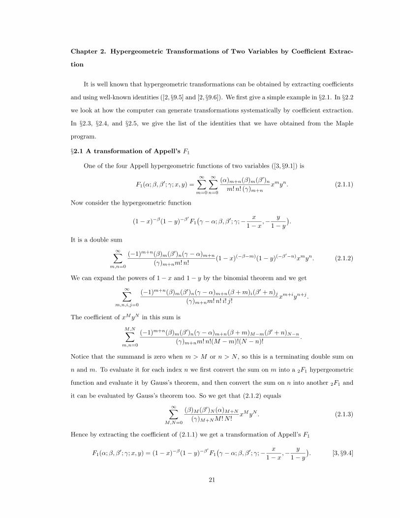
Chapter 2. Hypergeometric Transformations of Two Variables by Coefficient Extrac-

tion

It is well known that hypergeometric transformations can be obtained by extracting coefficients

and using well-known identities ([2, §9.5] and [2, §9.6]). We first give a simple example in §2.1. In §2.2

we look at how the computer can generate transformations systematically by coefficient extraction.

In §2.3, §2.4, and §2.5, we give the list of the identities that we have obtained from the Maple

program.

§2.1 A transformation of Appell’s F1

One of the four Appell hypergeometric functions of two variables ([3, §9.1]) is

F1(α;β, β′; γ;x, y) =∞∑

m=0

∞∑n=0

(α)m+n(β)m(β′)n

m!n! (γ)m+nxmyn. (2.1.1)

Now consider the hypergeometric function

(1− x)−β(1− y)−β′F1

(γ − α;β, β′; γ;− x

1− x,− y

1− y

).

It is a double sum

∞∑m,n=0

(−1)m+n(β)m(β′)n(γ − α)m+n

(γ)m+nm!n!(1− x)(−β−m)(1− y)(−β′−n)xmyn. (2.1.2)

We can expand the powers of 1− x and 1− y by the binomial theorem and we get

∞∑m,n,i,j=0

(−1)m+n(β)m(β′)n(γ − α)m+n(β + m)i(β′ + n)j

(γ)m+nm!n! i! j!xm+iyn+j .

The coefficient of xMyN in this sum is

M,N∑m,n=0

(−1)m+n(β)m(β′)n(γ − α)m+n(β + m)M−m(β′ + n)N−n

(γ)m+nm!n!(M −m)!(N − n)!.

Notice that the summand is zero when m > M or n > N , so this is a terminating double sum on

n and m. To evaluate it for each index n we first convert the sum on m into a 2F1 hypergeometric

function and evaluate it by Gauss’s theorem, and then convert the sum on n into another 2F1 and

it can be evaluated by Gauss’s theorem too. So we get that (2.1.2) equals

∞∑M,N=0

(β)M (β′)N (α)M+N

(γ)M+NM !N !xMyN . (2.1.3)

Hence by extracting the coefficient of (2.1.1) we get a transformation of Appell’s F1

F1(α;β, β′; γ;x, y) = (1− x)−β(1− y)−β′F1

(γ − α;β, β′; γ;− x

1− x,− y

1− y

). [3, §9.4]

21

§2.2 A systematic way to generate transformations

After we look at the way of getting the transformation in §2.1 more closely, it is clear that

the whole procedure, from a known double sum (2.1.2) to a new one (2.1.3) is just a routine which

can be done by computer. So the computer can always start with an arbitrary double sum of the

type (2.1.1), then perform the same routines as we did in the previous section and try to get a new

double sum of the type (2.1.3). Similar to the method in chapter 1, we can use partitions with

various cutoffs to generate such arbitrary double sums for the computer to start with.

Let’s illustrate the process with an example. We start with a formal power series in x and y

(1− x)p (1− y)q∑m,n

(a)m+n(b)m(c)n

m!n! (d)n(e)m

(− x

1− x

)m(− y

1− y

)n

.

Notice that this double sum corresponds to the partition {(1, 1), (1, 0), (0, 1), (0,−1), (−1, 0)},

which has cutoff (2, 1; 2, 1). The program first applies the procedure gather to combine the powers

of x, y, 1 − x and 1 − y then uses binexpand to expand powers of 1 − x and 1 − y by the binomial

theorem. After this it applies extract to get the coefficient of xM and yN , so the original sum

equals ∑M,N

∑m,n

(−1)m+n(a)m+n(−p + m)−m+M (b)m(−q + n)−n+N (c)n

m!n! (−m + M)! (−n + N)! (d)n(e)mxMyN .

The coefficient of xMyN is a terminating double sum in m and n. For each index n the program

first converts the corresponding sum in m into a hypergeometric series as

∑n

(−1)n (a)n(−p)M (−q + n)−n+N (c)n

n!M ! (−n + N)! (d)n3F2

(−M,a + n, b

−p, e

∣∣∣∣1) .

We would like to choose the parameters so that the 3F2 can be evaluated. Since only one parameter

a+n has the summation index n the numerators and denominators of the 3F2 cannot be adjusted to

make it balanced. So Saalschutz’s theorem cannot be applied. The only choice is Gauss’s theorem.

The program needs to reduce, through cancellation, the number of both the numerator and the

denominator parameters of the 3F2 by 1. The numerator parameter, b and the denominator param-

eters −p and e can be used for that purpose. Since canceling b with e is equivalent to canceling b

with −p and then setting e = −p this will just give some identities which are special cases of the

identities we get from setting b = −p. So we just have one way to do the cancellation, namely setting

b = −p. After cancellation and evaluating the resulting 2F1 by Gauss’s theorem the coefficient of

xMyN is a hypergeometric series in n,

(−p)M (−q)N (e− a)M

M !N ! (d)M4F3

(−N, a, c, 1− e + a

d,−q, 1− e−M + a

∣∣∣∣1) .

22

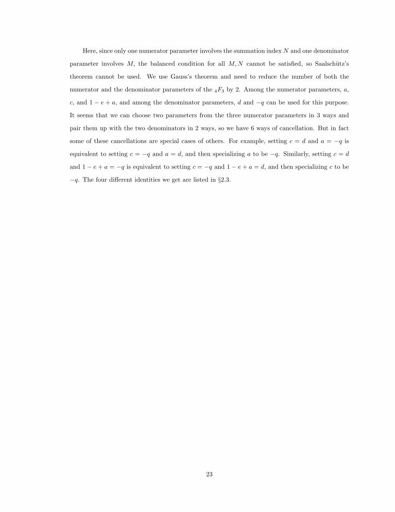
Here, since only one numerator parameter involves the summation index N and one denominator

parameter involves M, the balanced condition for all M,N cannot be satisfied, so Saalschutz’s

theorem cannot be used. We use Gauss’s theorem and need to reduce the number of both the

numerator and the denominator parameters of the 4F3 by 2. Among the numerator parameters, a,

c, and 1 − e + a, and among the denominator parameters, d and −q can be used for this purpose.

It seems that we can choose two parameters from the three numerator parameters in 3 ways and

pair them up with the two denominators in 2 ways, so we have 6 ways of cancellation. But in fact

some of these cancellations are special cases of others. For example, setting c = d and a = −q is

equivalent to setting c = −q and a = d, and then specializing a to be −q. Similarly, setting c = d

and 1− e + a = −q is equivalent to setting c = −q and 1− e + a = d, and then specializing c to be

−q. The four different identities we get are listed in §2.3.

23

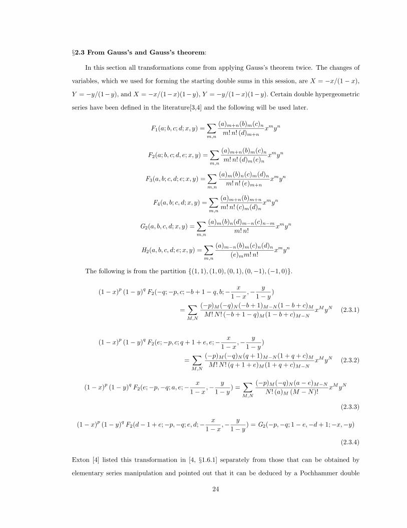
§2.3 From Gauss’s and Gauss’s theorem:

In this section all transformations come from applying Gauss’s theorem twice. The changes of

variables, which we used for forming the starting double sums in this session, are X = −x/(1− x),

Y = −y/(1−y), and X = −x/(1−x)(1−y), Y = −y/(1−x)(1−y). Certain double hypergeometric

series have been defined in the literature[3,4] and the following will be used later.

F1(a; b, c; d;x, y) =∑m,n

(a)m+n(b)m(c)n

m!n! (d)m+nxmyn

F2(a; b, c; d, e;x, y) =∑m,n

(a)m+n(b)m(c)n

m!n! (d)m(e)nxmyn

F3(a, b; c, d; e;x, y) =∑m,n

(a)m(b)n(c)m(d)n

m!n! (e)m+nxmyn

F4(a, b; c, d;x, y) =∑m,n

(a)m+n(b)m+n

m!n! (c)m(d)nxmyn

G2(a, b, c, d;x, y) =∑m,n

(a)m(b)n(d)m−n(c)n−m

m!n!xmyn

H2(a, b, c, d; e;x, y) =∑m,n

(a)m−n(b)m(c)n(d)n

(e)mm!n!xmyn

The following is from the partition {(1, 1), (1, 0), (0, 1), (0,−1), (−1, 0)}.

(1− x)p (1− y)q F2(−q;−p, c;−b + 1− q, b;− x

1− x,− y

1− y)

=∑M,N

(−p)M (−q)N (−b + 1)M−N (1− b + c)M

M !N ! (−b + 1− q)M (1− b + c)M−NxMyN (2.3.1)

(1− x)p (1− y)q F2(e;−p, c; q + 1 + e, e;− x

1− x,− y

1− y)

=∑M,N

(−p)M (−q)N (q + 1)M−N (1 + q + c)M

M !N ! (q + 1 + e)M (1 + q + c)M−NxMyN (2.3.2)

(1− x)p (1− y)q F2(e;−p,−q; a, e;− x

1− x,− y

1− y) =

∑M,N

(−p)M (−q)N (a− e)M−N

N ! (a)M (M −N)!xMyN

(2.3.3)

(1− x)p (1− y)q F2(d− 1 + e;−p,−q; e, d;− x

1− x,− y

1− y) = G2(−p,−q; 1− e,−d + 1;−x,−y)

(2.3.4)

Exton [4] listed this transformation in [4, §1.6.1] separately from those that can be obtained by

elementary series manipulation and pointed out that it can be deduced by a Pochhammer double

24

loop integral for G2. We now have shown that this transformation can also be obtained by means

of elementary series manipulations.

(1− x)p (1− y)q H2(b− e,−q,−p, e, b,− y

1− y,

x

1− x) = H2(−b + 1,−p,−q, e,−b + 1 + e, x,−y)

(2.3.5)

The following is from the partition {(1, 0), (0, 1), (1, 0), (0, 1), (−1,−1)}.

(1− x)p (1− y)q F3(−p, b; e,−q; e + b;− x

1− x,− y

1− y) = F3(−p,−q; b, e; e + b;x, y) (2.3.6)

The following is from the partition {(−1,−1), (0, 1), (1, 0), (1, 1)}.

(1− x)p (1− y)q F1(−q;−p, b; a;− x

1− x,− y

1− y)∑M,N

(−p)M (−q)N (a + q)M (a− b)M+N

M !N ! (a)M+N (a− b)MxMyN

(2.3.7)

(1− x)p (1− y)q F1(d;−p,−q; a;− x

1− x,− y

1− y) = F1(a− d;−p,−q; a;x, y) (2.3.8)

This transformation appears in [3, §9.4], where Bailey got it by evaluating on integral by change

of variables. The following is from the partition {(1,−1), (−1, 1), (1, 0), (0, 1)}.

(1− x)p (1− y)q G2(−p,−q; 1− a, c;x

1− x,

y

1− y) = F2(a− c;−p,−q; a, 1− c;x, y) (2.3.9)

(1− x)p (1− y)q G2(−p, 1− c; 1− a, c;x

1− x,

y

1− y) =

∑M,N

(−p)M (a− c)M (−q − 1 + a)M+N

M !N ! (a)M (−q − 1 + a)MxMyN

(2.3.10)

The right hand side of the above sum can be evaluated by binomial theorem and reduced to a single

sum. What we get is

(1− x)p (1− y)q G2(−p, 1−c; 1−a, c;x

1− x,

y

1− y) = (1− y)q+1−a

2F1

(−p, a− c

a

∣∣∣∣ x

1− y

)(2.3.11)

This one is from the partition {(−1, 0), (0,−1), (1, 1), (1, 1)}.

(1− x)p (1− y)q F4(−p,−q; a, b;− x

(1− x) (1− y),− y

(1− y) (1− x))

=∑M,N

(1− b− p)M (−p)M (a + q)M−N (−q)N (1− a− q)N

M !N ! (a)M (1− b− p)M−N (b)NxMyN (2.3.12)

This transformation is used by Bailey to prove another transformation. See [3, §9.6].

25

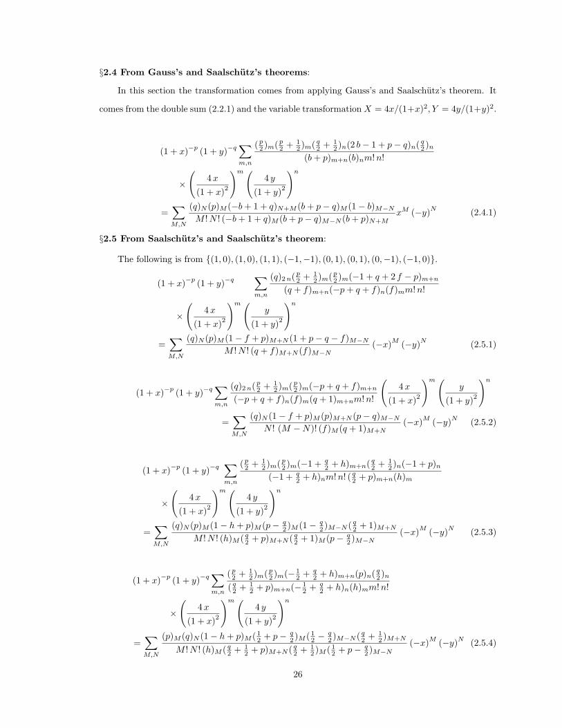
§2.4 From Gauss’s and Saalschutz’s theorems:

In this section the transformation comes from applying Gauss’s and Saalschutz’s theorem. It

comes from the double sum (2.2.1) and the variable transformation X = 4x/(1+x)2, Y = 4y/(1+y)2.

(1 + x)−p (1 + y)−q∑m,n

(p2 )m(p

2 + 12 )m( q

2 + 12 )n(2 b− 1 + p− q)n( q

2 )n

(b + p)m+n(b)nm!n!

×

(4 x

(1 + x)2

)m(4 y

(1 + y)2

)n

=∑M,N

(q)N (p)M (−b + 1 + q)N+M (b + p− q)M (1− b)M−N

M !N ! (−b + 1 + q)M (b + p− q)M−N (b + p)N+MxM (−y)N (2.4.1)

§2.5 From Saalschutz’s and Saalschutz’s theorem:

The following is from {(1, 0), (1, 0), (1, 1), (−1,−1), (0, 1), (0, 1), (0,−1), (−1, 0)}.

(1 + x)−p (1 + y)−q∑m,n

(q)2 n(p2 + 1

2 )m(p2 )m(−1 + q + 2 f − p)m+n

(q + f)m+n(−p + q + f)n(f)mm!n!

×

(4 x

(1 + x)2

)m(y

(1 + y)2

)n

=∑M,N

(q)N (p)M (1− f + p)M+N (1 + p− q − f)M−N

M !N ! (q + f)M+N (f)M−N(−x)M (−y)N (2.5.1)

(1 + x)−p (1 + y)−q∑m,n

(q)2 n(p2 + 1

2 )m(p2 )m(−p + q + f)m+n

(−p + q + f)n(f)m(q + 1)m+nm!n!

(4 x

(1 + x)2

)m(y

(1 + y)2

)n

=∑M,N

(q)N (1− f + p)M (p)M+N (p− q)M−N

N ! (M −N)! (f)M (q + 1)M+N(−x)M (−y)N (2.5.2)

(1 + x)−p (1 + y)−q∑m,n

(p2 + 1

2 )m(p2 )m(−1 + q

2 + h)m+n( q2 + 1

2 )n(−1 + p)n

(−1 + q2 + h)nm!n! ( q

2 + p)m+n(h)m

×

(4 x

(1 + x)2

)m(4 y

(1 + y)2

)n

=∑M,N

(q)N (p)M (1− h + p)M (p− q2 )M (1− q

2 )M−N ( q2 + 1)M+N

M !N ! (h)M ( q2 + p)M+N ( q

2 + 1)M (p− q2 )M−N

(−x)M (−y)N (2.5.3)

(1 + x)−p (1 + y)−q∑m,n

(p2 + 1

2 )m(p2 )m(− 1

2 + q2 + h)m+n(p)n( q

2 )n

( q2 + 1

2 + p)m+n(− 12 + q

2 + h)n(h)mm!n!

×

(4 x

(1 + x)2

)m(4 y

(1 + y)2

)n

=∑M,N

(p)M (q)N (1− h + p)M ( 12 + p− q

2 )M ( 12 −

q2 )M−N ( q

2 + 12 )M+N

M !N ! (h)M ( q2 + 1

2 + p)M+N ( q2 + 1

2 )M ( 12 + p− q

2 )M−N

(−x)M (−y)N (2.5.4)

26

(1 + x)−p (1 + y)−q∑m,n

(p2 + 1

2 )m(p2 )m(2− 2 h + p)n( q

2 + 12 )m+n( q

2 )n

(h)m( q2 + 3

2 − h)nm!n! ( q2 + 3

2 − h + p)m+n

×

(4 x

(1 + x)2

)m(4 y

(1 + y)2

)n

=∑M,N

(p)M (q)N (1− h + p)M (− q2 + 3

2 − h + p)M (− 12 −

q2 + h)M−N (− 1

2 + q2 + h)M+N

M !N ! (h)M ( q2 + 3

2 − h + p)M+N (− 12 + q

2 + h)M (− q2 + 3

2 − h + p)M−N

× (−x)M (−y)N (2.5.5)

(1 + x)−p (1 + y)−q∑m,n

(p2 + 1

2 )m(p2 )m(1− 2 h + p)n( q

2 + 12 )n( q

2 )m+n

( q2 + 1− h)n(h)mm!n! ( q

2 + 1− h + p)m+n

×

(4 x

(1 + x)2

)m(4 y

(1 + y)2

)n

=∑M,N

(p)M (q)N (1− h + p)M (− q2 + 1− h + p)M (− q

2 + h)M−N ( q2 + h)M+N

M !N ! (h)M ( q2 + 1− h + p)M+N ( q

2 + h)M (− q2 + 1− h + p)M−N

× (−x)M (−y)N (2.5.6)

§2.6 Identification of the transformations

Our program actually generates far more identities than what we have listed here. But most

of them are special cases of others, and we give an example to show why this is so. We start with

a double sum which corresponds to the partition {(−1,−1), (0,−1), (0, 1), (0, 1), (0, 1), (1, 0), (1, 0)}.

Following the same procedure as in §2.2 after first applying Gauss’s theorem to the coefficient, it

produces a hypergeometric series in n,

(q)N (p)M (1 + p− a)M (−1)NxMyN

M !N ! (a)M6F5

(−N, q + N, c, g, h, a− p

q2 , q

2 + 12 , b, a + M,a− p−M

∣∣∣∣1) .

To apply Saalschutz’s theorem the program enforces the balanced condition for the numerator and

denominator parameters, which is a + b − c − d − 1 = 0 and tries to reduce the 6F5 to a 3F2.

Numerator parameters c, g, h, and a− p, and denominator parameters q2 , q

2 + 12 , and b can be used

for the reduction. There are(43

)ways to choose the numerator parameters and 3! ways to pair them

up with the denominator parameters for cancellation, hence the number of identities is expected

to be 24. But in the end we just listed one identity in §2.4. Let’s look at the reasons that reduce

the number of identities. First, we need to eliminate identical identities due to the symmetry in

numerator or denominator parameters. In this case since the numerator parameters c, g, h are three

symmetric parameters, if two or all three are chosen then all permutations among them give the

27

same identities. And since at least two of the three symmetric parameters should be chosen for

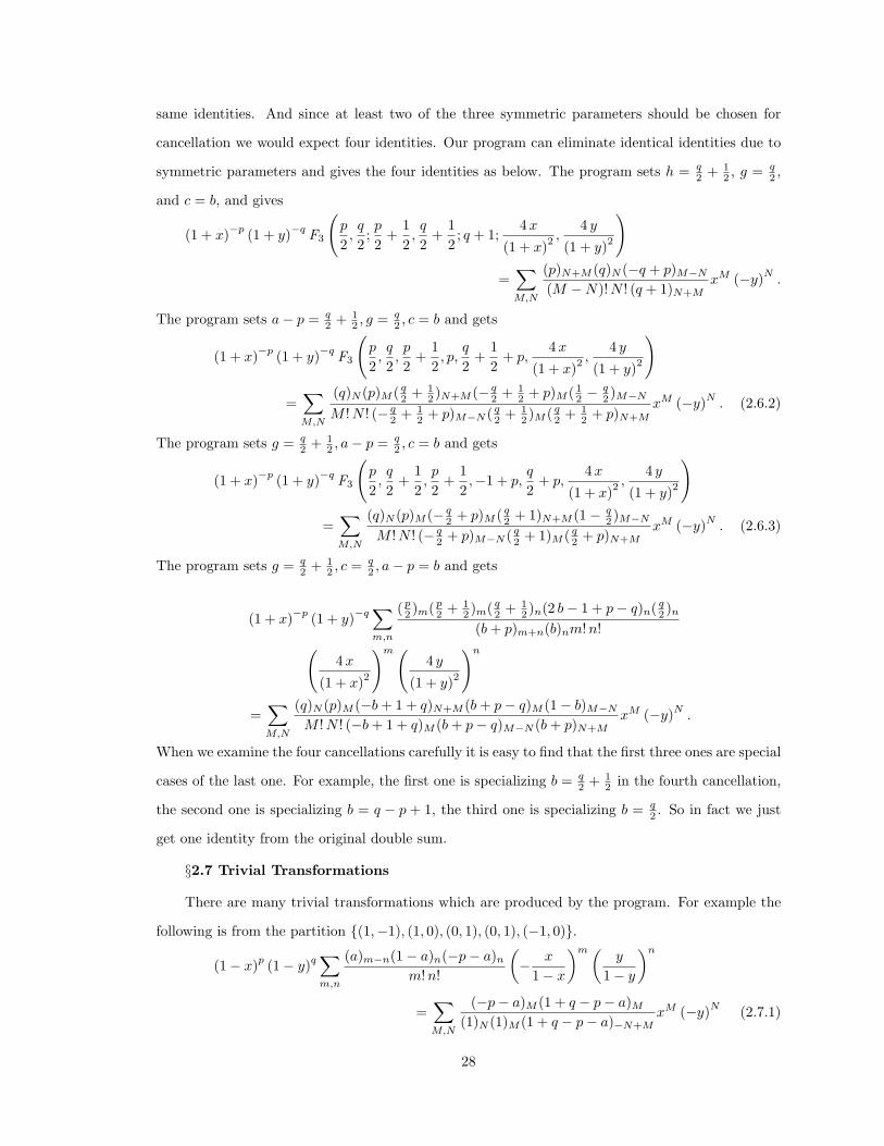
cancellation we would expect four identities. Our program can eliminate identical identities due to

symmetric parameters and gives the four identities as below. The program sets h = q2 + 1

2 , g = q2 ,

and c = b, and gives

(1 + x)−p (1 + y)−q F3

(p

2,q

2;p

2+

12,q

2+

12; q + 1;

4 x

(1 + x)2,

4 y

(1 + y)2

)

=∑M,N

(p)N+M (q)N (−q + p)M−N

(M −N)!N ! (q + 1)N+MxM (−y)N

.

The program sets a− p = q2 + 1

2 , g = q2 , c = b and gets

(1 + x)−p (1 + y)−q F3

(p

2,q

2,p

2+

12, p,

q

2+

12

+ p,4 x

(1 + x)2,

4 y

(1 + y)2

)

=∑M,N

(q)N (p)M ( q2 + 1

2 )N+M (− q2 + 1

2 + p)M ( 12 −

q2 )M−N

M !N ! (− q2 + 1

2 + p)M−N ( q2 + 1

2 )M ( q2 + 1

2 + p)N+M

xM (−y)N. (2.6.2)

The program sets g = q2 + 1

2 , a− p = q2 , c = b and gets

(1 + x)−p (1 + y)−q F3

(p

2,q

2+

12,p

2+

12,−1 + p,

q

2+ p,

4 x

(1 + x)2,

4 y

(1 + y)2

)

=∑M,N

(q)N (p)M (− q2 + p)M ( q

2 + 1)N+M (1− q2 )M−N

M !N ! (− q2 + p)M−N ( q

2 + 1)M ( q2 + p)N+M

xM (−y)N. (2.6.3)

The program sets g = q2 + 1

2 , c = q2 , a− p = b and gets

(1 + x)−p (1 + y)−q∑m,n

(p2 )m(p

2 + 12 )m( q

2 + 12 )n(2 b− 1 + p− q)n( q

2 )n

(b + p)m+n(b)nm!n!(4 x

(1 + x)2

)m(4 y

(1 + y)2

)n

=∑M,N

(q)N (p)M (−b + 1 + q)N+M (b + p− q)M (1− b)M−N

M !N ! (−b + 1 + q)M (b + p− q)M−N (b + p)N+MxM (−y)N

.

When we examine the four cancellations carefully it is easy to find that the first three ones are special

cases of the last one. For example, the first one is specializing b = q2 + 1

2 in the fourth cancellation,

the second one is specializing b = q − p + 1, the third one is specializing b = q2 . So in fact we just

get one identity from the original double sum.

§2.7 Trivial Transformations

There are many trivial transformations which are produced by the program. For example the

following is from the partition {(1,−1), (1, 0), (0, 1), (0, 1), (−1, 0)}.

(1− x)p (1− y)q∑m,n

(a)m−n(1− a)n(−p− a)n

m!n!

(− x

1− x

)m(y

1− y

)n

=∑M,N

(−p− a)M (1 + q − p− a)M

(1)N (1)M (1 + q − p− a)−N+MxM (−y)N (2.7.1)

28

Both sides can be evaluated by applying the binomial theorem twice and both reduce to

(1− y)q−p−a(1− x + xy)p+a.

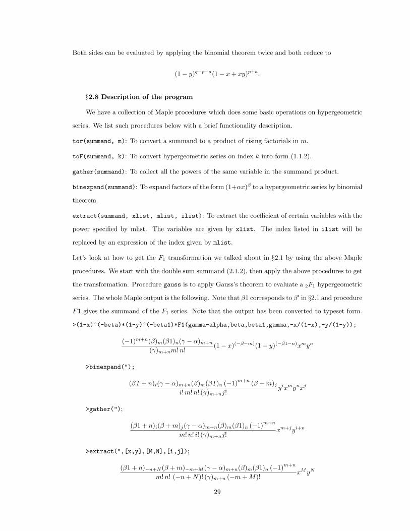
§2.8 Description of the program

We have a collection of Maple procedures which does some basic operations on hypergeometric

series. We list such procedures below with a brief functionality description.

tor(summand, m): To convert a summand to a product of rising factorials in m.

toF(summand, k): To convert hypergeometric series on index k into form (1.1.2).

gather(summand): To collect all the powers of the same variable in the summand product.

binexpand(summand): To expand factors of the form (1+αx)β to a hypergeometric series by binomial

theorem.

extract(summand, xlist, mlist, ilist): To extract the coefficient of certain variables with the

power specified by mlist. The variables are given by xlist. The index listed in ilist will be

replaced by an expression of the index given by mlist.

Let’s look at how to get the F1 transformation we talked about in §2.1 by using the above Maple

procedures. We start with the double sum summand (2.1.2), then apply the above procedures to get

the transformation. Procedure gauss is to apply Gauss’s theorem to evaluate a 2F1 hypergeometric

series. The whole Maple output is the following. Note that β1 corresponds to β′ in §2.1 and procedure

F1 gives the summand of the F1 series. Note that the output has been converted to typeset form.

>(1-x)^(-beta)*(1-y)^(-beta1)*F1(gamma-alpha,beta,beta1,gamma,-x/(1-x),-y/(1-y));

(−1)m+n(β)m(β1)n(γ − α)m+n

(γ)m+nm!n!(1− x)(−β−m)(1− y)(−β1−n)xmyn

>binexpand(");

(β1 + n)i(γ − α)m+n(β)m(β1 )n (−1)m+n (β + m)j

i!m!n! (γ)m+nj!yixmynxj

>gather(");

(β1 + n)i(β + m)j(γ − α)m+n(β)m(β1)n (−1)m+n

m!n! i! (γ)m+nj!xm+jyi+n

>extract(",[x,y],[M,N],[i,j]);

(β1 + n)−n+N (β + m)−m+M (γ − α)m+n(β)m(β1)n (−1)m+n

m!n! (−n + N)! (γ)m+n (−m + M)!xMyN

29

>toF(",m);

(β1 + n)−n+N (β)M (γ − α)n(β1)n (−1)n2F1

(γ−α+n,−M

γ+n

∣∣∣∣1)n! (−n + N)! (γ)nΓ(M + 1)

xMyN

>gauss(");

(β1 + n)−n+N (β)M (γ − α)n(β1 )n (−1)n Γ(γ + n)Γ(α + M)n! (−n + N)! (γ)nΓ(M + 1)Γ(α)Γ(γ + n + M)

xMyN

>toF(",n);

(β1)N (β)MΓ(γ)Γ(α + M)2F1

(γ−α,−N

γ+M

∣∣∣∣1)Γ(N + 1)Γ(M + 1)Γ(α)Γ(γ + M)

xMyN

>gauss(");(β1)N (β)MΓ(γ)Γ(M + N + α)

Γ(N + 1)Γ(M + 1)Γ(α)Γ(γ + M + N)xMyN

>tor(",M,N);(β1)N (β)M (α)M+N

(1)N (1)M (γ)M+NxMyN

The following carry out the systematic procedures (see §2.2) to generate the transformations.

createsummand: To create the partitions needed to generate the starting double sums. This is a

skeleton procedure which we modify to generate partitions with different cutoffs. For example to

generate partitions with cutoff (2, 1; 2, 1), we modify this procedure to become ggcreatesummand.

The name is due to the fact that most of the partitions form a double sum that require applying

Gauss’s theorem twice to give a transformation. Similarly with procedure gscreatesummand. The

s here refers to Saalschutz’s theorem.

get iden: To apply combinations of well known theorems to get the transformation. Just like

createsummand this is a skeleton procedure and is modified to different procedures which will try

applying different combinations of theorems.

30

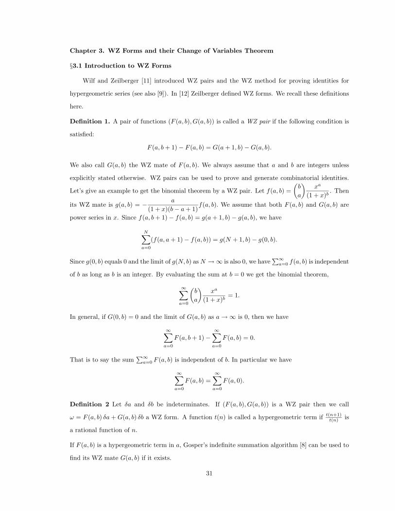
Chapter 3. WZ Forms and their Change of Variables Theorem

§3.1 Introduction to WZ Forms

Wilf and Zeilberger [11] introduced WZ pairs and the WZ method for proving identities for

hypergeometric series (see also [9]). In [12] Zeilberger defined WZ forms. We recall these definitions

here.

Definition 1. A pair of functions (F (a, b), G(a, b)) is called a WZ pair if the following condition is

satisfied:

F (a, b + 1)− F (a, b) = G(a + 1, b)−G(a, b).

We also call G(a, b) the WZ mate of F (a, b). We always assume that a and b are integers unless

explicitly stated otherwise. WZ pairs can be used to prove and generate combinatorial identities.

Let’s give an example to get the binomial theorem by a WZ pair. Let f(a, b) =(

b

a

)xa

(1 + x)b. Then

its WZ mate is g(a, b) = − a

(1 + x)(b− a + 1)f(a, b). We assume that both F (a, b) and G(a, b) are

power series in x. Since f(a, b + 1)− f(a, b) = g(a + 1, b)− g(a, b), we have

N∑a=0

(f(a, a + 1)− f(a, b)) = g(N + 1, b)− g(0, b).

Since g(0, b) equals 0 and the limit of g(N, b) as N →∞ is also 0, we have∑∞

a=0 f(a, b) is independent

of b as long as b is an integer. By evaluating the sum at b = 0 we get the binomial theorem,

∞∑a=0

(b

a

)xa

(1 + x)b= 1.

In general, if G(0, b) = 0 and the limit of G(a, b) as a →∞ is 0, then we have

∞∑a=0

F (a, b + 1)−∞∑

a=0

F (a, b) = 0.

That is to say the sum∑∞

a=0 F (a, b) is independent of b. In particular we have

∞∑a=0

F (a, b) =∞∑

a=0

F (a, 0).

Definition 2 Let δa and δb be indeterminates. If (F (a, b), G(a, b)) is a WZ pair then we call

ω = F (a, b) δa + G(a, b) δb a WZ form. A function t(n) is called a hypergeometric term if t(n+1)t(n) is

a rational function of n.

If F (a, b) is a hypergeometric term in a, Gosper’s indefinite summation algorithm [8] can be used to

find its WZ mate G(a, b) if it exists.

31

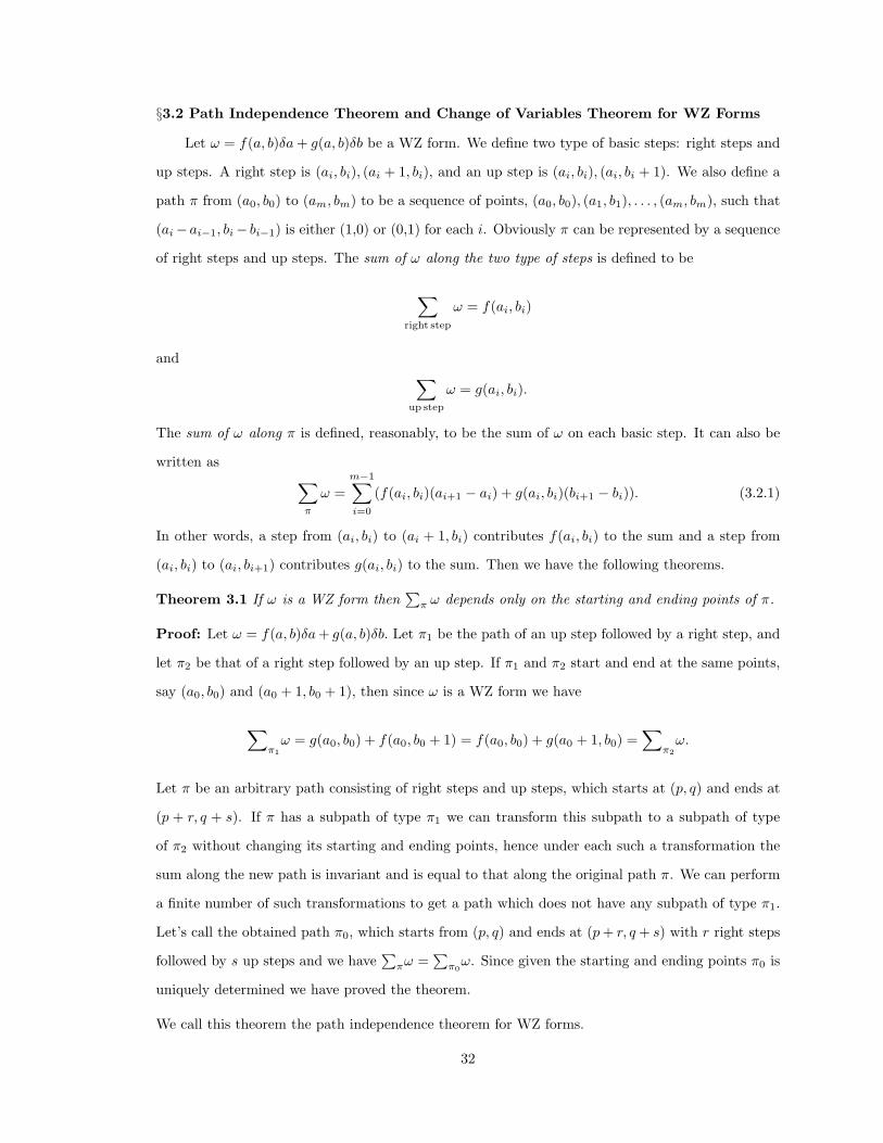
§3.2 Path Independence Theorem and Change of Variables Theorem for WZ Forms

Let ω = f(a, b)δa + g(a, b)δb be a WZ form. We define two type of basic steps: right steps and

up steps. A right step is (ai, bi), (ai + 1, bi), and an up step is (ai, bi), (ai, bi + 1). We also define a

path π from (a0, b0) to (am, bm) to be a sequence of points, (a0, b0), (a1, b1), . . . , (am, bm), such that

(ai−ai−1, bi− bi−1) is either (1,0) or (0,1) for each i. Obviously π can be represented by a sequence

of right steps and up steps. The sum of ω along the two type of steps is defined to be

∑right step

ω = f(ai, bi)

and ∑up step

ω = g(ai, bi).

The sum of ω along π is defined, reasonably, to be the sum of ω on each basic step. It can also be

written as ∑π

ω =m−1∑i=0

(f(ai, bi)(ai+1 − ai) + g(ai, bi)(bi+1 − bi)). (3.2.1)

In other words, a step from (ai, bi) to (ai + 1, bi) contributes f(ai, bi) to the sum and a step from

(ai, bi) to (ai, bi+1) contributes g(ai, bi) to the sum. Then we have the following theorems.

Theorem 3.1 If ω is a WZ form then∑

π ω depends only on the starting and ending points of π.

Proof: Let ω = f(a, b)δa + g(a, b)δb. Let π1 be the path of an up step followed by a right step, and

let π2 be that of a right step followed by an up step. If π1 and π2 start and end at the same points,

say (a0, b0) and (a0 + 1, b0 + 1), then since ω is a WZ form we have

∑π1

ω = g(a0, b0) + f(a0, b0 + 1) = f(a0, b0) + g(a0 + 1, b0) =∑

π2ω.

Let π be an arbitrary path consisting of right steps and up steps, which starts at (p, q) and ends at

(p + r, q + s). If π has a subpath of type π1 we can transform this subpath to a subpath of type

of π2 without changing its starting and ending points, hence under each such a transformation the

sum along the new path is invariant and is equal to that along the original path π. We can perform

a finite number of such transformations to get a path which does not have any subpath of type π1.

Let’s call the obtained path π0, which starts from (p, q) and ends at (p + r, q + s) with r right steps

followed by s up steps and we have∑

πω =∑

π0ω. Since given the starting and ending points π0 is

uniquely determined we have proved the theorem.

We call this theorem the path independence theorem for WZ forms.

32

Theorem 3.2 Suppose that ω = f(a, b)δa + g(a, b)δb is a WZ form. Then for any positive integers

r, s, t, u [ (r(a+1)+sb,t(a+1)+ub)∑(ra+sb,ta+ub)

ω

]δa +

[ (ra+s(b+1),ta+u(b+1))∑(ra+sb,ta+ub)

ω

]δb

is a WZ form.

Proof: Let

F (a, b) =(r(a+1)+sb,t(a+1)+ub)∑

(ra+sb,ta+ub)

ω

and

G(a, b) =(ra+s(b+1),ta+u(b+1))∑

(ra+sb,ta+ub)

ω.

We sum ω along two paths starting from (ra + sb, ta + ub) and ending at (r(a + 1) + s(b + 1), t(a +

1) + u(b + 1)). By Theorem 3.1 the sum is independent of the chosen paths so we may choose the

path to pass through the point (r(a + 1) + sb, t(a + 1) + ub). We have:

[ (r(a+1)+s(b+1),t(a+1)+u(b+1))∑(ra+sb,ta+ub)

ω

]=[ (r(a+1)+sb,t(a+1)+ub)∑

(ra+sb,ta+ub)

ω

]+[ (r(a+1)+s(b+1),t(a+1)+u(b+1))∑

(r(a+1)+sb,t(a+1)+ub)

ω

]= F (a, b) + G(a + 1, b)

.

If we choose the path to pass through the point (ra + s(b + 1), ta + u(b + 1)) we have

[ (r(a+1)+s(b+1),t(a+1)+u(b+1))∑(ra+sb,ta+ub)

ω

]=[ (ra+s(b+1),ta+u(b+1))∑

(ra+sb,ta+ub)

ω

]+[ (r(a+1)+s(b+1),t(a+1)+u(b+1))∑

(ra+s(b+1),ta+u(b+1))

ω

]= G(a, b) + F (a, b + 1)

.

So (F (a, b), G(a, b)) is a WZ pair and ω is a WZ form.

We call this theorem the change of variables theorem for WZ forms.

In (3.2.1) we have defined the sum of a WZ form along the paths which consist of right and up

steps. Now define two more types of basic step: a left step as (ai, bi), (ai − 1, bi), and a down step

as (ai, bi), (ai, bi − 1). We define the sum of the WZ form ω along these two steps by

∑left step

ω = −f(ai − 1, bi)

∑down step

ω = −g(ai, bi − 1).

With this definition we can extend the definition of the sum of ω along any path π, which is a

sequence of the four type of basic steps, to be the sum of ω on each step of ω. It is obvious that

33

the change of variables theorem generalizes to such paths as π. Moreover, we can define the sum

of ω along (ai, bi), (ai + 1, bi + 1) to be f(ai, bi) + g(ai + 1, bi), along (ai, bi), (ai + 1, bi − 1) to be

f(ai, bi)− g(ai + 1, bi − 1), along (ai, bi), (ai − 1, bi − 1) to be −f(ai − 1, bi)− g(ai − 1, bi − 1) and

along (ai, bi), (ai − 1, bi + 1) to be −f(ai − 1, bi) + g(ai − 1, bi). With such definition, the type of

steps of π can to extended to include the four types of diagonal steps and the path independence

theorem still holds on such paths.

§3.3 Examples of Path Independence Theorem

In this section we start with the WZ pair for Gauss’s theorem with numerator parameters

differing by a half. We first show how to get Gauss’s theorem by summing this WZ form on a path,

then we’ll show how summing along other paths gives other identities.

Let F1, · · · , Fn be n functions of variables a1, · · · , an. For any i, j, we can think of (Fi, Fj) as

functions of ai and aj with other variables fixed. If for all i, j, (Fi, Fj) is a WZ pair then we call

ω = F1δa1 + · · ·+Fnδan a WZ form in a1, · · · , an. In all the cases that we are interested in, it is easy

to show that if for all i (F1, Fi) is a WZ pair then for all i, j, (Fi, Fj) is also a WZ pair. We define the

sum of ω along a step (a1, · · · , ai, · · · , an), (a1, · · · , ai +1, · · · , an) to be Fi(a1, · · · , ai, · · · , an). We also

define the sum of ω along a step (a1, · · · , ai, · · · , an), (a1, · · · , ai − 1, · · · , an) to be −Fi(a1, · · · , ai −

1, · · · , an). With this definition, the path independence theorem holds true for n−variable WZ forms

and the proof is similar to the path independence theorem in two variables. For the sum of ω on an

arbitrary step, we can always define it to be the sum along a path which has the same starting and

ending point and consists only of the two types of steps on which we just defined the sum of ω.

The following is Gauss’s theorem with numerator parameters differing by a half:

2F1

(c2 , c

2 + 12

c + 12 + b

∣∣∣∣1)

=2c+2 b−1Γ(b)Γ(c + 1

2 + b)√

πΓ(c + 2 b), (3.3.1)

where c is a nonpositive integer. If we expand the hypergeometric series in (3.3.1) with summation

index a then divide each summand by the right hand side of (3.3.1) then (3.3.1) may be written as

∑a

Fa = 1

where

Fa =√

πΓ(c + 2 b)Γ(c + 2 a)21−2a−2b−c

Γ(a + c + 12 + b)Γ(c)Γ(1 + a)Γ(b)

.

With Gosper’s algorithm we can find Fb, and Fc such that (Fa, Fb) and (Fa, Fc) are WZ pairs, and

it follows that (Fb, Fc) is a WZ pair, so Faδa + Fbδb + Fcδc is a WZ form. We can leave out the

34

constant factor 2√

π in Fa and the WZ form in three variables we get is

2−2a−2b−cΓ(c + 2 b)Γ(c + 2 a)Γ(1 + a)Γ(b)Γ(c)Γ(a + c + 1

2 + b)δa

+2−2a−2b−cΓ(c + 2 b)Γ(c + 2 a)

Γ(a)Γ(b + 1)Γ(c)Γ(a + c + 12 + b)

δb

− 21−2a−2b−cΓ(c + 2 b)Γ(c + 2 a)Γ(a)Γ(b)Γ(1 + c)Γ(a + c + 1

2 + b)δc. (3.3.2)

Now we show how we can derive (3.3.1) when c is a nonpositive integer, say −n, with this WZ form

using the path independence theorem. Suppose n is a nonnegative even integer. We pick a path

from (0, b,−n) to (n2 + 1, b,−n) with (1, 0, 0) steps, then from (n

2 + 1, b,−n) to (n2 + 1, b, 0) with all

(0, 0, 1) steps, then from (n2 + 1, b, 0) to (0, b, 0) with all (−1, 0, 0) steps, then back to the starting

point (0, b,−n) with all (0, 0,−1) steps. The sum of the WZ form from (0, b,−n) to (n2 +1, b,−n) is

Γ(2 b− n)2n−2 b

Γ(−n + 12 + b)Γ(b) 2F1

(−n

2 ,−n2 + 1

2

−n + 12 + b

∣∣∣∣1)

. (3.3.3)

The sum of the WZ form from (n2 + 1, b,−n) to (n

2 + 1, b, 0) is

−1∑c=−n

2−c−2 bΓ(c + 2 b)( c2 )n

2 +1( c2 + 1

2 )n2 +1

Γ(b + 1)Γ(n2 + 1)Γ(c + 1

2 + b)(c + 12 + b)n

2 +1

.

Since ( c2 )n

2 +1( c2 + 1)n

2 +1 is always 0, so the sum above is equal to 0. The sum on the steps from

(n2 + 1, b, 0) to (0, b, 0) is

−n2∑

a=0

Γ(2 b)2−2 b(0)a( 12 )a

Γ(b)Γ(b + 12 )(1)a(b + 1

2 )a

.

The summand is 0 except when a = 0 so the sum of the WZ form by the duplication formula

for the gamma function is

− Γ(2 b)2−2 b

Γ(b + 12 )Γ(b)

= − 12√

π.

The sum on steps from (0, b, 0) back to (0, b,−n) is

−−n∑c=0

2−c−2 bΓ(c + 2 b)( c2 )0( c

2 + 12 )0

Γ(b + 1)Γ(0)Γ(c + 12 + b)(c + 1

2 + b)0.

The sum is 0 due to Γ(0) in the denominator of the summand. By the path independence theorem,

the sum on the whole path is 0, so we get

Γ(c + 2 b)2−c−2 b

Γ(c + 12 + b)Γ(b) 2F1

(c2 , c

2 + 12

c + 12 + b

∣∣∣∣1)

=1

2√

π.

After dividing all the extra factors to leave only the 2F1 on the left side of the equation, we get

(3.3.1). Similarly, we can prove the case when n is odd.

35

We use the term segment to refer to the connected section of a path which consists of the most

possible same type of steps. So the path we chose above has four segments. Our observation is

that the sum of the WZ form gives a hypergeometric series with some coefficient on one segment

of the path. The sum on the parallel segment is the evaluation of that hypergeometric series with

the coefficient at one of the parameters of the hypergeometric series equal to 0. As a result, the

hypergeometric series has only one nonzero term which is 1. Thus the evaluation is a constant.

Moreover, the terms of the sum of the WZ form on the other two parallel segments are all 0, hence,

indicating the value of the hypergeometric series is a constant. In our following examples, all the

paths we choose give us an evaluation of a hypergeometric series in the same manner.

Now we look at the sum of the WZ forms on different type of steps. The sum on step (a, b, c +

i), (a, b, c + i + 1) is

− 21−c−i−2a−2bΓ(c + i + 2 b)Γ(c + i + 2 a)Γ(c + i + 1)Γ(a)Γ(a + c + i + 1

2 + b)Γ(b).

When c equals 0, summing on i gives a hypergeometric series

−Γ(a + 1

2 )Γ(b + 12 )

2 π Γ(a + b + 12 ) 2F1

(2 b, 2 a

a + b + 12

∣∣∣∣12)

. (3.3.4)

By setting a to be a nonpositive integer, say −n, we get a terminating hypergeometric series

−( 12 − b)n

2√

π( 12 )n

2F1

(2 b,−2 n

−n + b + 12

∣∣∣∣12)

. (3.3.5)

Furthermore we pick the following path which shows that the terminating hypergeometric series

sums to a constant value. The path goes from (−n, b, 0) to (−n, b, 2n + 1) with all (0, 0, 1) steps

which gives us (3.3.5), then to (0, b, 2n+1) with (1, 0, 0) steps on which the WZ form is all 0, then to

(0, b, 0) with all (0, 0,−1) steps, the sum of the WZ form on which is the negative of the evaluation

of (3.3.4) at a = 0, then back to (−n, b, 0) with all (−1, 0, 0) steps on which the WZ form is again

all 0. Thus we have

2F1

(2 b,−2 n

−n + b + 12

∣∣∣∣12)

=( 12 )n

( 12 − b)n

.

Now we sum (3.3.2) on the step (a + i, b− i, c), (a + i + 1, b− i− 1, c). We get

−Γ(c + 2 b− 2− 2 i)Γ(c + 2 a + 2 i) (−b + 2 i + 1 + a) 22−2 a−2 b−c

Γ(c)Γ(a + i + 1)Γ(b− i)Γ(a− 12 + c + b)

.

When a = 0, summing on i we get

−Γ(c + 2 b− 2) (1− b) 22−2 b−c

Γ(b)Γ(− 12 + c + b) 4F3

(c2 , c

2 + 12 , 1− b, 3

2 −b2

32 −

c2 − b, 2− c

2 − b, 12 −

b2

∣∣∣∣− 1

).

36

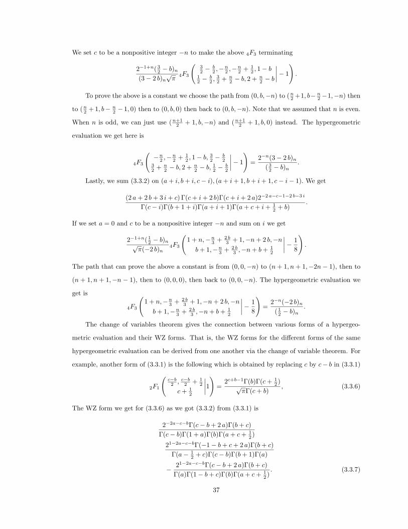
We set c to be a nonpositive integer −n to make the above 4F3 terminating

2−1+n( 32 − b)n

(3− 2 b)n√

π4F3

(32 −

b2 ,−n

2 ,−n2 + 1

2 , 1− b12 −

b2 , 3

2 + n2 − b, 2 + n

2 − b

∣∣∣∣− 1

).

To prove the above is a constant we choose the path from (0, b,−n) to (n2 +1, b− n

2 −1,−n) then

to (n2 + 1, b− n

2 − 1, 0) then to (0, b, 0) then back to (0, b,−n). Note that we assumed that n is even.

When n is odd, we can just use (n+12 + 1, b,−n) and (n+1

2 + 1, b, 0) instead. The hypergeometric

evaluation we get here is

4F3

(−n

2 ,−n2 + 1

2 , 1− b, 32 −

b2

32 + n

2 − b, 2 + n2 − b, 1

2 −b2

∣∣∣∣− 1

)=

2−n(3− 2 b)n

( 32 − b)n

.

Lastly, we sum (3.3.2) on (a + i, b + i, c− i), (a + i + 1, b + i + 1, c− i− 1). We get

(2 a + 2 b + 3 i + c) Γ(c + i + 2 b)Γ(c + i + 2 a)2−2 a−c−1−2 b−3 i

Γ(c− i)Γ(b + 1 + i)Γ(a + i + 1)Γ(a + c + i + 12 + b)

.

If we set a = 0 and c to be a nonpositive integer −n and sum on i we get

2−1+n( 12 − b)n√

π(−2 b)n4F3

(1 + n,−n

3 + 2 b3 + 1,−n + 2 b,−n

b + 1,−n3 + 2 b

3 ,−n + b + 12

∣∣∣∣− 18

).

The path that can prove the above a constant is from (0, 0,−n) to (n + 1, n + 1,−2n− 1), then to

(n + 1, n + 1,−n − 1), then to (0, 0, 0), then back to (0, 0,−n). The hypergeometric evaluation we

get is

4F3

(1 + n,−n

3 + 2 b3 + 1,−n + 2 b,−n

b + 1,−n3 + 2 b

3 ,−n + b + 12

∣∣∣∣− 18

)=

2−n(−2 b)n

( 12 − b)n

.

The change of variables theorem gives the connection between various forms of a hypergeo-

metric evaluation and their WZ forms. That is, the WZ forms for the different forms of the same

hypergeometric evaluation can be derived from one another via the change of variable theorem. For

example, another form of (3.3.1) is the following which is obtained by replacing c by c− b in (3.3.1)

2F1

(c−b2 , c−b

2 + 12

c + 12

∣∣∣∣1)

=2c+b−1Γ(b)Γ(c + 1

2 )√

πΓ(c + b), (3.3.6)

The WZ form we get for (3.3.6) as we got (3.3.2) from (3.3.1) is

2−2a−c−bΓ(c− b + 2 a)Γ(b + c)Γ(c− b)Γ(1 + a)Γ(b)Γ(a + c + 1

2 )

21−2a−c−bΓ(−1− b + c + 2 a)Γ(b + c)Γ(a− 1

2 + c)Γ(c− b)Γ(b + 1)Γ(a)

− 21−2a−c−bΓ(c− b + 2 a)Γ(b + c)Γ(a)Γ(1− b + c)Γ(b)Γ(a + c + 1

2 ). (3.3.7)

37

If we use change of variables theorem to compute the new WZ form for (3.3.2) under the change of

variables a → a, b → b, c → c− b we also get (3.3.7).

§3.4 WZ forms of linear hypergeometric transformations

Finding the WZ mate for a linear hypergeometric transformation is not trivial. For example,

we take Euler’s transformation

(1− x)b+c−d2F1

(b, c

d

∣∣∣∣x) = 2F1

(d− b, d− c

d

∣∣∣∣x) . (3.4.1)

We divide the left side summand by the right side and get

F (a, b) =(1− x)b+c−d (b)a(c)a

(d)a

xa

a!

2F1

(d− b, d− c

d

∣∣∣∣x) . (3.4.2)

Gosper’s algorithm cannot find a WZ mate G(a, b) for F (a, b), such that F (a, b+1)−F (a, b) =

G(a + 1, b) − G(a, b). In fact, F (a, b) is not even a hypergeometric term. If we make a change of

variables c = d + m, assuming that m is an integer, then the summand becomes

F (a, b) =(1− x)b+m (b)a(d + m)a

(d)a

xa

a!

2F1

(d− b,−m

d

∣∣∣∣x) , (3.4.3)

which can also be written as

F (a, b) =Γ(b + a)xa(1− x)b+m(d + m)a

Γ(b)Γ(a + 1)2F1

(d− b,−m

d

∣∣∣∣x) .

Now if we let m = 1, the denominator is a polynomial in b, so F (a, b) is a hypergeometric term.

Applying Gosper’s algorithm we get the WZ mate for (3.4.3)

−Γ(b + a)xa(1− x)b+1(d + a)3F2

(d− b, d + a− 1,−1

d, d + a

∣∣∣∣x)Γ(b + 1)Γ(a) d 2F1

(d− b,−1

d

∣∣∣∣x) 2F1

(d− b− 1,−1

d

∣∣∣∣x) . (3.4.4)

The WZ mate turns out to have a nice formula and it motivated us to look at more values of m in

the hope that we can find a general form for the WZ mate for (3.4.3). When m = 2 we have the

WZ mate for (3.4.3)

−Γ(b + a)xa(1− x)b+2(d + a)2 3F2

(d− b, d + a− 1,−2

d, d + a

∣∣∣∣x)Γ(b + 1)Γ(a)(d)2 2F1

(d− b,−2

d

∣∣∣∣x) 2F1

(d− b− 1,−2

d

∣∣∣∣x) . (3.4.5)

38

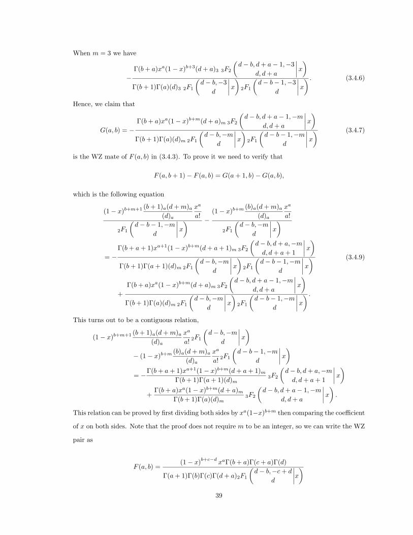
When m = 3 we have

−Γ(b + a)xa(1− x)b+3(d + a)3 3F2

(d− b, d + a− 1,−3

d, d + a

∣∣∣∣x)Γ(b + 1)Γ(a)(d)3 2F1

(d− b,−3

d

∣∣∣∣x) 2F1

(d− b− 1,−3

d

∣∣∣∣x) . (3.4.6)

Hence, we claim that

G(a, b) = −Γ(b + a)xa(1− x)b+m(d + a)m 3F2

(d− b, d + a− 1,−m

d, d + a

∣∣∣∣x)Γ(b + 1)Γ(a)(d)m 2F1

(d− b,−m

d

∣∣∣∣x) 2F1

(d− b− 1,−m

d

∣∣∣∣x) (3.4.7)

is the WZ mate of F (a, b) in (3.4.3). To prove it we need to verify that

F (a, b + 1)− F (a, b) = G(a + 1, b)−G(a, b),

which is the following equation

(1− x)b+m+1 (b + 1)a(d + m)a

(d)a

xa

a!

2F1

(d− b− 1,−m

d

∣∣∣∣x) −(1− x)b+m (b)a(d + m)a

(d)a

xa

a!

2F1

(d− b,−m

d

∣∣∣∣x)

= −Γ(b + a + 1)xa+1(1− x)b+m(d + a + 1)m 3F2

(d− b, d + a,−m

d, d + a + 1

∣∣∣∣x)Γ(b + 1)Γ(a + 1)(d)m 2F1

(d− b,−m

d

∣∣∣∣x) 2F1

(d− b− 1,−m

d

∣∣∣∣x)

+Γ(b + a)xa(1− x)b+m(d + a)m 3F2

(d− b, d + a− 1,−m

d, d + a

∣∣∣∣x)Γ(b + 1)Γ(a)(d)m 2F1

(d− b,−m

d

∣∣∣∣x) 2F1

(d− b− 1,−m

d

∣∣∣∣x) .

(3.4.9)

This turns out to be a contiguous relation,

(1− x)b+m+1 (b + 1)a(d + m)a

(d)a

xa

a! 2F1

(d− b,−m

d

∣∣∣∣x)− (1− x)b+m (b)a(d + m)a

(d)a

xa

a! 2F1

(d− b− 1,−m

d

∣∣∣∣x)= −Γ(b + a + 1)xa+1(1− x)b+m(d + a + 1)m

Γ(b + 1)Γ(a + 1)(d)m3F2

(d− b, d + a,−m

d, d + a + 1

∣∣∣∣x)+

Γ(b + a)xa(1− x)b+m(d + a)m

Γ(b + 1)Γ(a)(d)m3F2

(d− b, d + a− 1,−m

d, d + a

∣∣∣∣x) .

This relation can be proved by first dividing both sides by xa(1−x)b+m then comparing the coefficient

of x on both sides. Note that the proof does not require m to be an integer, so we can write the WZ

pair as

F (a, b) =(1− x)b+c−d

xaΓ(b + a)Γ(c + a)Γ(d)

Γ(a + 1)Γ(b)Γ(c)Γ(d + a)2F1

(d− b,−c + d

d

∣∣∣∣x)39

and

G(a, b) = − (1− x)b+c−dxaΓ(b + a)Γ(c + a)Γ(d)

Γ(a)Γ(b + 1)Γ(c)Γ(d + a)

3F2

(d− b, d + a− 1,−c + d

d, d + a

∣∣∣∣x)2F1

(d− b,−c + d

d

∣∣∣∣x) 2F1

(d− b− 1,−c + d

d

∣∣∣∣x) .

It is easy to see that, if (f(a, b), g(a, b)) is a WZ pair, then (−f(−a − 1, b), g(−a, b)) is also a

WZ pair [5]. For example, the WZ pair for binomial theorem is

f(a, b) =Γ(b + 1)xa

Γ(a + 1)Γ(b− a + 1) (1 + x)b,

and

g(a, b) = − aΓ(b + 1)xa

(b− a + 1)Γ(a + 1)Γ(b− a + 1) (1 + x)b+1.

So the following is a new WZ pair,

f ′(a, b) = −f(−a− 1, b) = − Γ(b + 1)x−a−1

Γ(−a)Γ(b + a + 2) (1 + x)b,

and

g′(a, b) = g(−a, b) =aΓ(b + 1)x−a

(b + a + 1) Γ(−a + 1)Γ(b + a + 1) (1 + x)b+1.

When a is a nonnegative integer, f ′(a, b) is zero. To make a more interesting WZ pair out of

(f ′(a, b), g′(a, b)) we recall another method that a new pair of WZ form is derived from an existing

WZ pair in [5]. If p(a, b) is a function such that p(a+1, b) = p(a, b+1) = p(a, b) for all complex a and

b for which p(a, b) is defined then (p(a, b)F (a, b), p(a, b)G(a, b)) is a WZ-pair. Clearly (F (a,b)p(a,b) , G(a,b)

p(a,b) )

is also a WZ-pair. One such p(a, b) is (−1)sa+tb[sinπ(sa+ tb)]/π, where (−1)α is defined to be eiπα.

By the reflection formula for the gamma function, we have Γ(sa+tb)Γ(1−sa−tb) = π/ sinπ(sa+tb).

So p(a, b) can also be expressed as

p(a, b) =(−1)sa+tb

Γ(sa + tb)Γ(1− sa− tb).

So we can multiply both f ′(a, b) and g′(a, b) by

Γ(−a)Γ(1 + a)(−1)−a

and the new WZ pair we get is

f ′′(a, b) = − (−1)−a Γ(b + 1)Γ(a + 1)x−a−1

Γ(b + a + 2) (1 + x)b

and

g′′(a, b) = − (−1)−a Γ(b + 1)Γ(a + 1)x−a

Γ(b + a + 2) (1 + x)1+b.

40

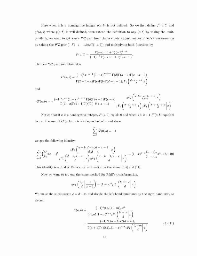
Here when a is a nonnegative integer p(a, b) is not defined. So we first define f ′′(a, b) and

g′′(a, b) where p(a, b) is well defined, then extend the definition to any (a, b) by taking the limit.

Similarly, we want to get a new WZ pair from the WZ pair we just got for Euler’s transformation

by taking the WZ pair (−F (−a− 1, b), G(−a, b)) and multiplying both functions by

P (a, b) =Γ(−a)Γ(a + 1) (−1)b−a

(−1)−a Γ(−b + a + 1)Γ(b− a).

The new WZ pair we obtained is

F ′(a, b) =(−1)bx−a−1 (1− x)b+c−d Γ(d)Γ(a + 1)Γ(c− a− 1)

Γ(2− b + a)Γ(c)Γ(b)Γ(d− a− 1)2F1

(d−b,−c+d

d

∣∣∣∣x)and

G′(a, b) = − (−1)bx−a (1− x)b+c−d Γ(d)Γ(a + 1)Γ(c− a)Γ(d− a)Γ(b + 1)Γ(c)Γ(−b + a + 1)

3F2

(d−b,d−a−1,−c+d

d,d−a

∣∣∣∣x)2F1

(d−b,−c+d

d

∣∣∣∣x) 2F1

(d−b−1,−c+d

d

∣∣∣∣x) .

Notice that if a is a nonnegative integer, F ′(a, 0) equals 0 and when b > a + 1 F ′(a, b) equals 0

too, so the sum of G′(a, b) on b is independent of n and since

∞∑b=0

G′(0, b) = −1

we get the following identity

a∑b=0

(a

b

)(x−1)b

3F2

(d− b, d− c, d− a− 1

d, d− a

∣∣∣∣ x)2F1

(d− b, d− c

d

∣∣∣∣ x) 2F1

(d− b− 1, d− c

d

∣∣∣∣ x) = (1−x)d−c (1− c)a

(1− d)axa. (3.4.10)

This identity is a dual of Euler’s transformation in the sense of [5] and [11].

Now we want to try out the same method for Pfaff’s transformation,

2F1

(b, c

d

∣∣∣∣ x

x− 1

)= (1− x)b

2F1

(b, d− c

d

∣∣∣∣x) .

We make the substitution c = d + m and divide the left hand summand by the right hand side, so

we get

F (a, b) =(−1)a(b)a(d + m)axa

(d)aa! (1− x)a+b2F1

(b,−m

d

∣∣∣∣x)=

(−1)aΓ(a + b)xa(d + m)a

Γ(a + 1)Γ(b)(d)a(1− x)a+b2F1

(b,−m

d

∣∣∣∣x) (3.4.11)

41

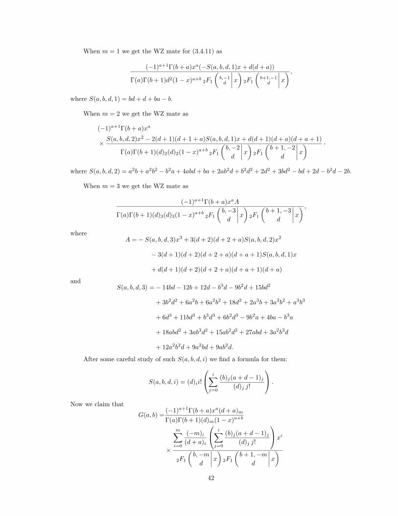
When m = 1 we get the WZ mate for (3.4.11) as

(−1)a+1Γ(b + a)xa(−S(a, b, d, 1)x + d(d + a))

Γ(a)Γ(b + 1)d2(1− x)a+b2F1

(b,−1

d

∣∣∣∣x) 2F1

(b+1,−1

d

∣∣∣∣x) ,

where S(a, b, d, 1) = bd + d + ba− b.

When m = 2 we get the WZ mate as

(−1)a+1Γ(b + a)xa

× S(a, b, d, 2)x2 − 2(d + 1)(d + 1 + a)S(a, b, d, 1)x + d(d + 1)(d + a)(d + a + 1)

Γ(a)Γ(b + 1)(d)2(d)2(1− x)a+b2F1

(b,−2

d

∣∣∣∣x) 2F1

(b + 1,−2

d

∣∣∣∣x),

where S(a, b, d, 2) = a2b + a2b2 − b2a + 4abd + ba + 2ab2d + b2d2 + 2d2 + 3bd2 − bd + 2d− b2d− 2b.

When m = 3 we get the WZ mate as

(−1)a+1Γ(b + a)xaA

Γ(a)Γ(b + 1)(d)3(d)3(1− x)a+b2F1

(b,−3

d

∣∣∣∣x) 2F1

(b + 1,−3

d

∣∣∣∣x) ,

whereA =− S(a, b, d, 3)x3 + 3(d + 2)(d + 2 + a)S(a, b, d, 2)x2

− 3(d + 1)(d + 2)(d + 2 + a)(d + a + 1)S(a, b, d, 1)x

+ d(d + 1)(d + 2)(d + 2 + a)(d + a + 1)(d + a)

andS(a, b, d, 3) =− 14bd− 12b + 12d− b3d− 9b2d + 15bd2

+ 3b2d2 + 6a2b + 6a2b2 + 18d2 + 2a3b + 3a3b2 + a3b3

+ 6d3 + 11bd3 + b3d3 + 6b2d3 − 9b2a + 4ba− b3a

+ 18abd2 + 3ab3d2 + 15ab2d2 + 27abd + 3a2b3d

+ 12a2b2d + 9a2bd + 9ab2d.

After some careful study of such S(a, b, d, i) we find a formula for them:

S(a, b, d, i) = (d)ii!

i∑j=0

(b)j(a + d− 1)j

(d)j j!

.

Now we claim that

G(a, b) =(−1)a+1Γ(b + a)xa(d + a)m

Γ(a)Γ(b + 1)(d)m(1− x)a+b

×

m∑i=0

(−m)i

(d + a)i

i∑j=0

(b)j(a + d− 1)j

(d)j j!

xi

2F1

(b,−m

d

∣∣∣∣x) 2F1

(b + 1,−m

d

∣∣∣∣x)42

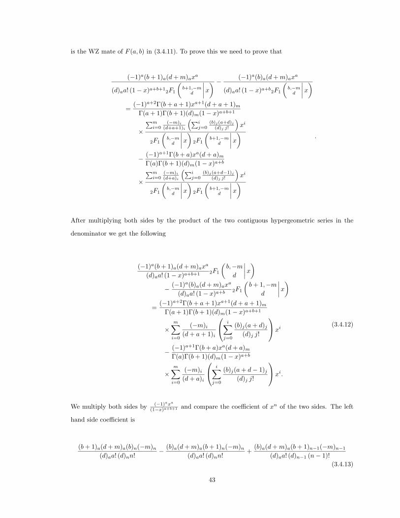
is the WZ mate of F (a, b) in (3.4.11). To prove this we need to prove that

(−1)a(b + 1)a(d + m)axa

(d)aa! (1− x)a+b+12F1

(b+1,−m

d

∣∣∣∣x) − (−1)a(b)a(d + m)axa

(d)aa! (1− x)a+b2F1

(b,−m

d

∣∣∣∣x)=

(−1)a+2Γ(b + a + 1)xa+1(d + a + 1)m

Γ(a + 1)Γ(b + 1)(d)m(1− x)a+b+1

×

∑mi=0

(−m)i

(d+a+1)i

(∑ij=0

(b)j(a+d)j

(d)j j!

)xi

2F1

(b,−m

d

∣∣∣∣x) 2F1

(b+1,−m

d

∣∣∣∣x)− (−1)a+1Γ(b + a)xa(d + a)m

Γ(a)Γ(b + 1)(d)m(1− x)a+b

×

∑mi=0

(−m)i

(d+a)i

(∑ij=0

(b)j(a+d−1)j

(d)j j!

)xi

2F1

(b,−m

d

∣∣∣∣x) 2F1

(b+1,−m

d

∣∣∣∣x)

.

After multiplying both sides by the product of the two contiguous hypergeometric series in the

denominator we get the following

(−1)a(b + 1)a(d + m)axa

(d)aa! (1− x)a+b+1 2F1

(b,−m

d

∣∣∣∣x)− (−1)a(b)a(d + m)axa

(d)aa! (1− x)a+b 2F1

(b + 1,−m

d

∣∣∣∣x)=

(−1)a+2Γ(b + a + 1)xa+1(d + a + 1)m

Γ(a + 1)Γ(b + 1)(d)m(1− x)a+b+1

×m∑

i=0

(−m)i

(d + a + 1)i

i∑j=0

(b)j(a + d)j

(d)j j!

xi

− (−1)a+1Γ(b + a)xa(d + a)m

Γ(a)Γ(b + 1)(d)m(1− x)a+b

×m∑

i=0

(−m)i

(d + a)i

i∑j=0

(b)j(a + d− 1)j

(d)j j!

xi.

(3.4.12)

We multiply both sides by (−1)axa

(1−x)a+b+1 and compare the coefficient of xn of the two sides. The left

hand side coefficient is

(b + 1)a(d + m)a(b)n(−m)n

(d)aa! (d)nn!− (b)a(d + m)a(b + 1)n(−m)n

(d)aa! (d)nn!+

(b)a(d + m)a(b + 1)n−1(−m)n−1

(d)aa! (d)n−1 (n− 1)!(3.4.13)

43

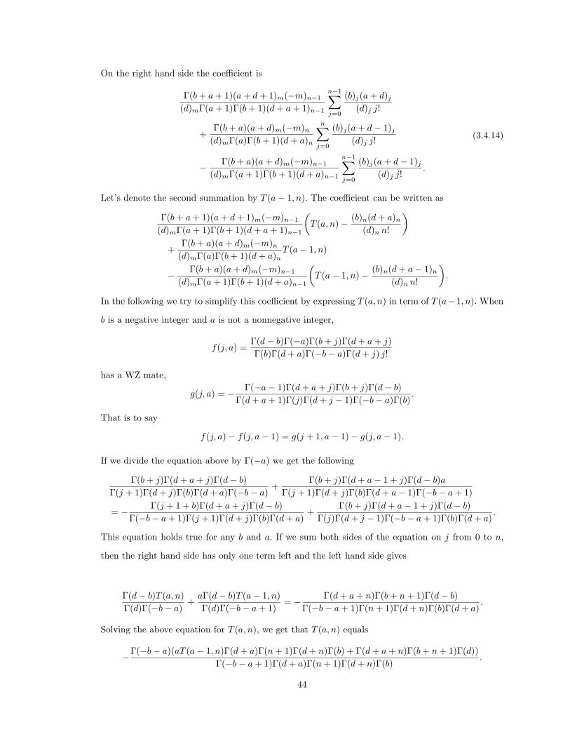
On the right hand side the coefficient is

Γ(b + a + 1)(a + d + 1)m(−m)n−1

(d)mΓ(a + 1)Γ(b + 1)(d + a + 1)n−1

n−1∑j=0

(b)j(a + d)j

(d)j j!

+Γ(b + a)(a + d)m(−m)n

(d)mΓ(a)Γ(b + 1)(d + a)n

n∑j=0

(b)j(a + d− 1)j

(d)j j!

− Γ(b + a)(a + d)m(−m)n−1

(d)mΓ(a + 1)Γ(b + 1)(d + a)n−1

n−1∑j=0

(b)j(a + d− 1)j

(d)j j!.

(3.4.14)

Let’s denote the second summation by T (a− 1, n). The coefficient can be written as

Γ(b + a + 1)(a + d + 1)m(−m)n−1

(d)mΓ(a + 1)Γ(b + 1)(d + a + 1)n−1

(T (a, n)− (b)n(d + a)n

(d)n n!

)+

Γ(b + a)(a + d)m(−m)n

(d)mΓ(a)Γ(b + 1)(d + a)nT (a− 1, n)

− Γ(b + a)(a + d)m(−m)n−1

(d)mΓ(a + 1)Γ(b + 1)(d + a)n−1

(T (a− 1, n)− (b)n(d + a− 1)n

(d)n n!

).

In the following we try to simplify this coefficient by expressing T (a, n) in term of T (a−1, n). When

b is a negative integer and a is not a nonnegative integer,

f(j, a) =Γ(d− b)Γ(−a)Γ(b + j)Γ(d + a + j)Γ(b)Γ(d + a)Γ(−b− a)Γ(d + j) j!

has a WZ mate,

g(j, a) = − Γ(−a− 1)Γ(d + a + j)Γ(b + j)Γ(d− b)Γ(d + a + 1)Γ(j)Γ(d + j − 1)Γ(−b− a)Γ(b)

.

That is to say

f(j, a)− f(j, a− 1) = g(j + 1, a− 1)− g(j, a− 1).

If we divide the equation above by Γ(−a) we get the following

Γ(b + j)Γ(d + a + j)Γ(d− b)Γ(j + 1)Γ(d + j)Γ(b)Γ(d + a)Γ(−b− a)

+Γ(b + j)Γ(d + a− 1 + j)Γ(d− b)a

Γ(j + 1)Γ(d + j)Γ(b)Γ(d + a− 1)Γ(−b− a + 1)

= − Γ(j + 1 + b)Γ(d + a + j)Γ(d− b)Γ(−b− a + 1)Γ(j + 1)Γ(d + j)Γ(b)Γ(d + a)

+Γ(b + j)Γ(d + a− 1 + j)Γ(d− b)

Γ(j)Γ(d + j − 1)Γ(−b− a + 1)Γ(b)Γ(d + a).

This equation holds true for any b and a. If we sum both sides of the equation on j from 0 to n,

then the right hand side has only one term left and the left hand side gives

Γ(d− b)T (a, n)Γ(d)Γ(−b− a)

+aΓ(d− b)T (a− 1, n)Γ(d)Γ(−b− a + 1)

= − Γ(d + a + n)Γ(b + n + 1)Γ(d− b)Γ(−b− a + 1)Γ(n + 1)Γ(d + n)Γ(b)Γ(d + a)

.

Solving the above equation for T (a, n), we get that T (a, n) equals

−Γ(−b− a)(aT (a− 1, n)Γ(d + a)Γ(n + 1)Γ(d + n)Γ(b) + Γ(d + a + n)Γ(b + n + 1)Γ(d))Γ(−b− a + 1)Γ(d + a)Γ(n + 1)Γ(d + n)Γ(b)

.

44

Thus, we can have expressed T (a, n) in term of T (a− 1, n), and we can write (3.4.14) as

Γ(b + a + 1)(a + d + 1)m(−m)n−1

(d)mΓ(a + 1)Γ(b + 1)(d + a + 1)n−1

×(− Γ(−b− a)(aT (a− 1, n)Γ(d + a)Γ(n + 1)Γ(d + n)Γ(b) + Γ(d + a + n)Γ(b + n + 1)Γ(d))

Γ(−b− a + 1)Γ(d + a)Γ(n + 1)Γ(d + n)Γ(b)

− (b)n(d + a)n

(d)n n!

)+

Γ(b + a)(a + d)m(−m)n

(d)mΓ(a)Γ(b + 1)(d + a)nT (a− 1, n)

− Γ(b + a)(a + d)m(−m)n−1

(d)mΓ(a + 1)Γ(b + 1)(d + a)n−1(T (a− 1, n)− (b)n(d + a− 1)n

(d)n n!).

(3.4.16)

The coefficient of T (a− 1, n) in (3.4.16) is

− Γ(b + a + 1)(a + d + 1)m(−m)n−1Γ(−b− a)a(d)mΓ(a + 1)(a + d + 1)n−1Γ(b + 1)Γ(−b− a + 1)

+Γ(b + a)(d + a)m(−m)n

(d)mΓ(a)Γ(b + 1)(d + a)n

− Γ(b + a)(d + a)m(−m)n−1

(d)mΓ(a)Γ(b + 1)(d + a)n−1.

The above reduces to 0 when we simplify it in Maple. Moreover, simplifying the difference (3.4.13)−

(3.4.16) in Maple gives 0. Hence we proved that the contiguous relation in (3.4.12) is true. Therefore,

we have proved that

G(a, b) =(−1)a+1Γ(b + a)xa(d + a)m

Γ(a)Γ(b + 1)(d)m(1− x)a+b

×

m∑i=0

(−m)i

(d + a)i

i∑j=0

(b)j(a + d− 1)j

(d)j j!

xi

2F1

(b,−m

d

∣∣∣∣x) 2F1

(b + 1,−m

d

∣∣∣∣x)is the WZ mate of

F (a, b) =(−1)aΓ(a + b)xa(d + m)a

Γ(a + 1)Γ(b)(d)a(1− x)a+b2F1

(b,−m

d

∣∣∣∣x) .

§3.5 Symmetric Function and Path Independence Theorem of WZ forms

So far all the WZ forms we studied are for hypergeometric functions. In this section we use the

symmetric function WZ pair defined in [7] and apply the path independence theorem to prove the

q-binomial identity in [6].

Let us define the complete symmetric functions hn in the variables u1, u2, · · · , um by

hn(u0, u1, · · · , um) =∑

0≤i1≤i2≤···≤in≤m

ui1ui2 · · ·uin ,

45

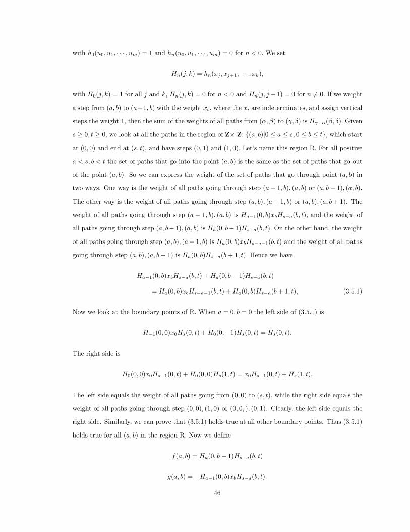
with h0(u0, u1, · · · , um) = 1 and hn(u0, u1, · · · , um) = 0 for n < 0. We set

Hn(j, k) = hn(xj , xj+1, · · · , xk),

with H0(j, k) = 1 for all j and k, Hn(j, k) = 0 for n < 0 and Hn(j, j− 1) = 0 for n 6= 0. If we weight

a step from (a, b) to (a+1, b) with the weight xb, where the xi are indeterminates, and assign vertical

steps the weight 1, then the sum of the weights of all paths from (α, β) to (γ, δ) is Hγ−α(β, δ). Given

s ≥ 0, t ≥ 0, we look at all the paths in the region of Z× Z: {(a, b)|0 ≤ a ≤ s, 0 ≤ b ≤ t}, which start

at (0, 0) and end at (s, t), and have steps (0, 1) and (1, 0). Let’s name this region R. For all positive

a < s, b < t the set of paths that go into the point (a, b) is the same as the set of paths that go out

of the point (a, b). So we can express the weight of the set of paths that go through point (a, b) in

two ways. One way is the weight of all paths going through step (a− 1, b), (a, b) or (a, b− 1), (a, b).

The other way is the weight of all paths going through step (a, b), (a + 1, b) or (a, b), (a, b + 1). The

weight of all paths going through step (a − 1, b), (a, b) is Ha−1(0, b)xbHs−a(b, t), and the weight of

all paths going through step (a, b− 1), (a, b) is Ha(0, b− 1)Hs−a(b, t). On the other hand, the weight

of all paths going through step (a, b), (a + 1, b) is Ha(0, b)xbHs−a−1(b, t) and the weight of all paths

going through step (a, b), (a, b + 1) is Ha(0, b)Hs−a(b + 1, t). Hence we have

Ha−1(0, b)xbHs−a(b, t) + Ha(0, b− 1)Hs−a(b, t)

= Ha(0, b)xbHs−a−1(b, t) + Ha(0, b)Hs−a(b + 1, t), (3.5.1)

Now we look at the boundary points of R. When a = 0, b = 0 the left side of (3.5.1) is

H−1(0, 0)x0Hs(0, t) + H0(0,−1)Hs(0, t) = Hs(0, t).

The right side is

H0(0, 0)x0Hs−1(0, t) + H0(0, 0)Hs(1, t) = x0Hs−1(0, t) + Hs(1, t).

The left side equals the weight of all paths going from (0, 0) to (s, t), while the right side equals the

weight of all paths going through step (0, 0), (1, 0) or (0, 0, ), (0, 1). Clearly, the left side equals the

right side. Similarly, we can prove that (3.5.1) holds true at all other boundary points. Thus (3.5.1)

holds true for all (a, b) in the region R. Now we define

f(a, b) = Ha(0, b− 1)Hs−a(b, t)

g(a, b) = −Ha−1(0, b)xbHs−a(b, t).

46

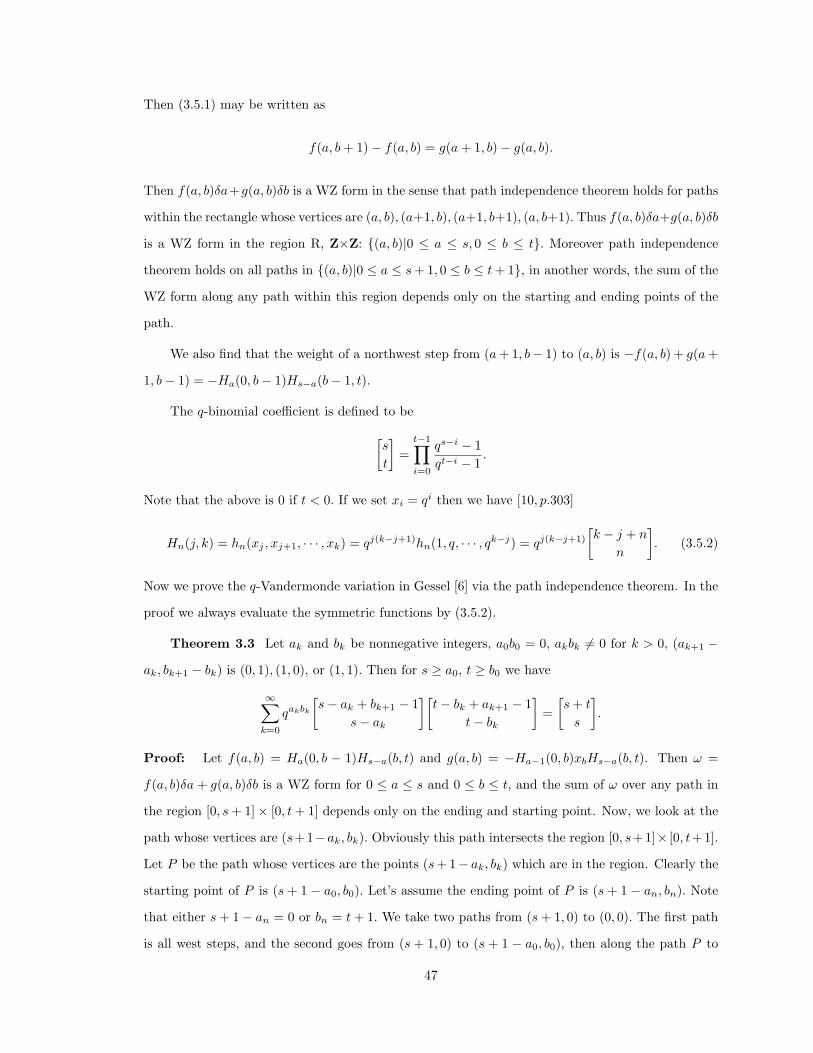
Then (3.5.1) may be written as

f(a, b + 1)− f(a, b) = g(a + 1, b)− g(a, b).

Then f(a, b)δa+g(a, b)δb is a WZ form in the sense that path independence theorem holds for paths

within the rectangle whose vertices are (a, b), (a+1, b), (a+1, b+1), (a, b+1). Thus f(a, b)δa+g(a, b)δb

is a WZ form in the region R, Z×Z: {(a, b)|0 ≤ a ≤ s, 0 ≤ b ≤ t}. Moreover path independence

theorem holds on all paths in {(a, b)|0 ≤ a ≤ s + 1, 0 ≤ b ≤ t + 1}, in another words, the sum of the

WZ form along any path within this region depends only on the starting and ending points of the

path.

We also find that the weight of a northwest step from (a + 1, b− 1) to (a, b) is −f(a, b) + g(a +

1, b− 1) = −Ha(0, b− 1)Hs−a(b− 1, t).

The q-binomial coefficient is defined to be[s

t

]=

t−1∏i=0

qs−i − 1qt−i − 1

.

Note that the above is 0 if t < 0. If we set xi = qi then we have [10, p.303]

Hn(j, k) = hn(xj , xj+1, · · · , xk) = qj(k−j+1)hn(1, q, · · · , qk−j) = qj(k−j+1)

[k − j + n

n

]. (3.5.2)

Now we prove the q-Vandermonde variation in Gessel [6] via the path independence theorem. In the

proof we always evaluate the symmetric functions by (3.5.2).

Theorem 3.3 Let ak and bk be nonnegative integers, a0b0 = 0, akbk 6= 0 for k > 0, (ak+1 −

ak, bk+1 − bk) is (0, 1), (1, 0), or (1, 1). Then for s ≥ a0, t ≥ b0 we have

∞∑k=0

qakbk

[s− ak + bk+1 − 1

s− ak

][t− bk + ak+1 − 1

t− bk

]=[s + t

s

].

Proof: Let f(a, b) = Ha(0, b − 1)Hs−a(b, t) and g(a, b) = −Ha−1(0, b)xbHs−a(b, t). Then ω =

f(a, b)δa + g(a, b)δb is a WZ form for 0 ≤ a ≤ s and 0 ≤ b ≤ t, and the sum of ω over any path in

the region [0, s + 1]× [0, t + 1] depends only on the ending and starting point. Now, we look at the

path whose vertices are (s+1−ak, bk). Obviously this path intersects the region [0, s+1]× [0, t+1].

Let P be the path whose vertices are the points (s + 1− ak, bk) which are in the region. Clearly the

starting point of P is (s + 1 − a0, b0). Let’s assume the ending point of P is (s + 1 − an, bn). Note

that either s + 1− an = 0 or bn = t + 1. We take two paths from (s + 1, 0) to (0, 0). The first path

is all west steps, and the second goes from (s + 1, 0) to (s + 1 − a0, b0), then along the path P to

47

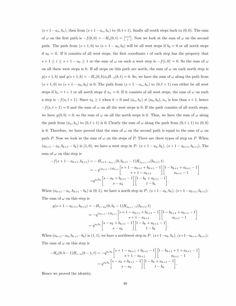
(s+1−an, bn), then from (s+1−an, bn) to (0, t+1), finally all south steps back to (0, 0). The sum

of ω on the first path is −f(0, 0) = −Hs(0, t) =[s+t

t

]. Now we look at the sum of ω on the second

path. The path from (s + 1, 0) to (s + 1 − a0, b0) will be all west steps if b0 = 0 or all north steps

if a0 = 0. If it consists of all west steps, the first coordinate i of each step has the property that

s + 1 ≥ i ≥ s + 1 − a0 ≥ 1 so the sum of ω on such a west step is −f(i, 0) = 0. So the sum of ω

on all these west steps is 0. If all steps on this path are north, the sum of ω on each north step is

g(s+1, b) and g(s+1, b) = −Hs(0, b)xbH−1(b, t) = 0. So, we have the sum of ω along the path from

(s + 1, 0) to (s + 1 − a0, b0) is 0. The path from (s + 1 − an, bn) to (0, t + 1) can either be all west

steps if bn = t + 1 or all north steps if an = 0. If it consists of all west steps, the sum of ω on such

a step is −f(a, t + 1). Since ak ≥ 1 when k > 0 and (an, bn) 6= (a0, b0), an is less than s + 1, hence

−f(a, t + 1) = 0 and the sum of ω on all the west steps is 0. If the path consists of all north steps,

we have g(0, b) = 0, so the sum of ω on all the north steps is 0. Thus, we have the sum of ω along

the path from (an, bn) to (0, t + 1) is 0. Clearly the sum of ω along the path from (0, t + 1) to (0, 0)

is 0. Therefore, we have proved that the sum of ω on the second path is equal to the sum of ω on

path P. Now we look at the sum of ω on the steps of P. There are three types of step on P. When

(ak+1 − ak, bk+1 − bk) is (1, 0), we have a west step in P : (s + 1− ak, bk), (s + 1− ak+1, bk+1). The

sum of ω on this step is

−f(s + 1− ak+1, bk+1) =−Hs+1−ak+1(0, bk+1 − 1)Hak+1−1(bk+1, t)

=− q(ak+1−1)bk+1

[s + 1− ak+1 + bk+1 − 1

s + 1− ak+1

][t− bk+1 + ak+1 − 1

ak+1 − 1

]=qakbk

[s− ak + bk+1 − 1

s− ak

][t− bk + ak+1 − 1

t− bk

].

When (ak+1−ak, bk+1− bk) is (0, 1), we have a north step in P : (s+1−ak, bk), (s+1−ak+1, bk+1).

The sum of ω on this step is

g(s + 1− ak+1, bk+1) = −Hs−ak(0, bk − 1)Hak+1−1(bk+1, t)

= −q(ak+1−1)bk+1

[s + 1− ak+1 + bk+1 − 1

s + 1− ak+1

][t− bk+1 + ak+1 − 1

ak+1 − 1

]= qakbk

[s− ak + bk+1 − 1

s− ak

][t− bk + ak+1 − 1

t− bk

].

When (ak+1−ak, bk+1−bk) is (1, 1), we have a northwest step in P : (s+1−ak, bk), (s+1−ak+1, bk+1).

The sum of ω on this step is

−Ha(0, b− 1)Hs−a(b− 1, t) = −qakbk

[s + 1− ak+1 + bk+1 − 1

s + 1− ak+1

][t− bk+1 + 1 + ak+1 − 1

ak+1 − 1

]= qakbk

[s− ak + bk+1 − 1

s− ak

][t− bk + ak+1 − 1

t− bk

].

Hence we proved the identity.

48

References

[1] T. Amdeberhan and D. Zeilberger, Hypergeometric series acceleration via the WZ Method, Elec-

tronic Journal of Combinatorics, 4 (1997).

[2] Bateman Manuscript Project–Higher Transcendental Functions, Vol. 1 (McGraw Hill, 1954).

[3] W. Bailey, Generalized Hypergeometric Series, (Cambridge University Press, New York, 1972).

[4] H. Exton, Multiple Hypergeometric Functions and Applications, (Ellis Horwood Ltd, 1976).

[5] I. M. Gessel, Finding identities with the WZ Method, J. Symbolic Computation, 20 (1995) 537–566.

[6] I. M. Gessel, Some generalized Durfee square identities, Discrete Math., 49 (1984), 41–44.

[7] I. M. Gessel, Combinatorial aspects of the WZ method, unpublished manuscript, (2001).

[8] R. W. Gosper Jr., Decision procedure for indefinite hypergeometric series, SIAM J. Math. Anal.,

12 (1978) 295–308.

[9] M. Petkovsek, H.S. Wilf, and D. Zeilberger, A = B, (A.K. Peters, Ltd., Wellesley, Mass., 1996).

[10] R. P. Stanley, Enumerative Combinatorics, Vol. 2, (Cambridge University Press, 1999).

[11] H.S. Wilf, and D. Zeilberger, Rational functions certify combinatorial identities, J. Amer. Math.

Soc. 3 (1990) 147–158.

[12] D. Zeilberger, Closed form (pun intended!) Contemporary Mathematics, 143 (1993) 579–607.

49