Applications of Computational Fluid Dynamics-based methods to problems in computational science

Computing Systems in Engineering Vol. 1, No. 1. pp. 7-22, 1990 0956-0521/90 $3.(~1+0.(~J Printed in Great Britain © 1991) Pergamon Press plc

APPLICATIONS OF COMPUTATIONAL FLUID DYNAMICS-BASED METHODS TO PROBLEMS IN COMPUTATIONAL SCIENCE

V. SHANKAR, W. F. HALL, A. H. MOHAMMADIAN and S. CHAKRAVARTHY

Rockwell International Science Center, Thousand Oaks, CA 91360, U.S.A.

(Received 10 April 1990)

Abstract--The objective is to describe how some of the attributes of Computational Fluid Dynamics (CFD) can be extended to solve mathematical problems in other disciplines, such as electromagnetics, that are,, governed by appropriate partial differential equations and boundary conditions. The concept of finite-w31ume schemes applied to the conservation forms of fluid dynamics equations, such as the Euler and Navier-Stokes equations, is readily extendable to other equations. For example, Maxwell's equations of electromagnetics, when cast in conservation form, can be easily solved using characteristic theory-based CFD methods allowing for a precise implementation of material interface and other boundary conditions.

The possibility of extending CFD-based methods to other disciplines has a special significance because increasingly the development of advanced aerospace systems requires a total integration of multidisciplinary technologies (aerodynamics, structures, propulsion, controls, low observables, etc.). Many of the computational issues such as (1) development of implicit/explicit, higher order accurate schemes, (2) complex geometry representation and setup of structured or unstructured grid cells, (3) vector/ massively parallel computer architectures and execution/memory requirements, (4) pre/post processing graphics, and (5) user interface/training requirements, are common to many disciplines.

The establishment of "Computational Science" to perform interdisciplinary coupled problems addressing many of the above computational issues can certainly benefit from the CFD experience.

It is hriefly explained how some of the CFD-based methods are applied to study scattering problems for radar cross section (RCS) studies, and simulation of laser/material interaction accounting for melting. Also mentioned are some of the interdisciplinary computations involving CFD, aeroelasticity, and controls. Future studies will include coupling of RCS and CFD in the design process.

INTRODUCTION

The deve lopment of modern aerospace vehicles increasingly requires synergism in integrating multidisciplinary technologies such as ( i ) fluid dynamics for flow management , (2) structures for flexibility effects, (3) propulsion for thrust, (4) controls for stability, and (5) low observables for stealth con- siderations. Implement ing such an integrated approach demands development of a computat ional envi ronment that encompasses many disciplines.

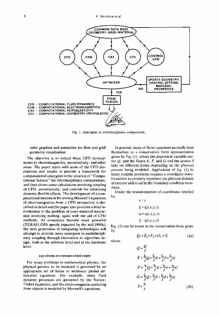
Along with rapid strides in algorithm and code deve lopment , the increasing power of supercomputers , superminicomputers , and graphics workstations is rapidly advancing the state of the art of computational simulation of problems in mathematical physics. One area that is setting the pace is Computa- tional Fluid Dynamics (CFD). Other disciplines such as Computat ional Electromagnetics (CEM) are starting to benefit from the C F D experience, as shown in Fig. 1, to achieve synergism in multidisciplinary computat ion. The thrust of this paper is to briefly describe the attributes of C F D and how some of them can be extended to other disciplines, especially CEM.

CFD has been evolving over the last 30 years, addressing the simulation of complex linear/nonlinear flow processes using advanced numerical techniques and state-of-the-art computers. Some of the attributes of C F D are listed here.

(1) The hierarchy of gas dynamics equations such as the full potential , Euler , and Navier -S tokes equat ions are usually cast in a conservation form as

Q,+Ex+F~+G~=source, (1)

where Q is the solution vector and E, F, and G are the fluxes in x, y, and z coordinate directions, respectively. The conservation form readily ad- mits weak solutions such as shock waves.

(2) Body-fitted coordinates are employed to represent the complex geometry topology and allow easy implementat ion of the boundary conditions.

(3) Numerical gridding procedures are used to set up ei ther structured or unstructured computat ional cells.

(4) Characteristics-based numerical algorithms are employed in developing upwind-biased, higher order accurate (space and time), stable, implicit or explicit schemes.

(5) Supercomputers employing both vector (CRAY-class) and massively parallel (hypercube) architecture are employed to solve the complex flow equat ions with current computing technology providing G I G A F L O P S (10 9 opera- tions/second) performance.

(6) Graphics workstations provide a versatile capa- bility for performing pre/post processing with

8 W. SHANKAR et al.

OMETRY, (~ OPTIMIZER ~ = I CONTROL SETTING,

t FINAL ]

DESIGN CFD - COMPUTATIONAL FLUID DYNAMICS t t

CEM - COMPUTATIONAL ELECTROMAGNETICS J L CAE COMPUTATIONAL AEROELASTICITY CCh COMPUTATIONAL CHEMISTRY (PROPULSION) 7 7 /

Fig. 1. Synergism in rnultidisciplinary computation.

color graphics and animation for flow and grid/ geometry visualization.

The objective is to extend these CFD develop- ments to electromagnetics, aeroelasticity, and other areas. The paper starts with some of the CFD des- criptions and results to provide a framework for computational synergism in the creation of "Compu- tational Science" for interdisciplinary computations, and then shows some calculations involving coupling of CFD, aeroelasticity, and controls for simulating dynamic flexible effects. The development of a computational treatment for solving Maxwell's equations of electromagnetics from a CFD perspective is described in detail and the paper also provides a brief introduction to the problem of laser-material interaction involving melting, again with the aid of CFD methods. As computers become more powerful (TERAFLOPS speeds expected by the mid-1990s), the next generation of computing technologies will attempt to provide more synergism in multidisciplinary coupling through innovation in algorithm design, both at the software level and at the hardware level.

EQUATIONS IN CONSERVATION FORM

For many problems in mathematical physics, the physical process to be modeled is governed by an appropriate set of linear or nonlinear partial differential equations. For example, many fluid dynamic processes are governed by the Navier- Stokes equations, and the electromagnetic scattering from objects is modeled by Maxwell's equations.

In general, many of these equations naturally lend themselves to a conservation form representation given by Eq. (1), where the dependent variable vector Q, and the fluxes E, F, and G and the source S take on different forms depending on the physical process being modeled. Application of Eq. (1) to many realistic problems requires a coordinate transformation to properly represent the physical domain of interest and to aid in the boundary condition treatment.

Under the transformation of coordinates implied by

T = t

= ~(t,x,y, z)

rl = "q( t,x, y,z)

= ~(t,x,y,z)

Eq. (1) can be recast in the conservation form given by

O.r + / ~ +/',~ + (~ = ,-¢, (2a) where

o=_Q J

E = ~Q+--jE+ J F + T G

[.= "q, Q+'q~E+ ~_~F+TbG J J J J

1~ = ~O+ ~ E + ~F+ ~ G J ~ J J J

$=s J

(2b)

Applications of CFD-based methods 9

where, in turn, J is the Jacobian of the transformation

J = O('r,~,'q,O/O(t,x,y,z ) (2c)

and ~,, ~x, ~y, ~z, vl,, rl~, Vly, "q~, ~,, ~x, ~, and ~ are the .transformation metrics.

Associating the subscripts j, k and I with the ~, ~q, and { directions as shown in Fig. 2, a numerical approximation to Eq. (2a) may be expressed in the semidiscrete conservation law form given by

+ (d, . , . ,+, ,2-dj . , . ,_ , ,~):0, (3)

where ~, P, and (~ are the numerical fluxes representing the physical fluxes E, [', and O at the bound- ing sides of the cell for which discrete conservation is considered, and 0~.,.t is the representative conserved quantity (the numerical approximation to Q) considered conveniently to be the centroidal value. The half-integer subscripts denote cell sides and the integer subscripts the cell itself or its centroid.

The semidiscrete conservation law form given by Eq. (3) may be regarded as representing a finite volume discretization because the Jacobian J appearing in 0 is associated with the volume of the cell (~.~J,.t = ( Q V ) , , j , V is the volume), and the metrics ~/J, ~,./J, and so on appearing in the flux terms are nothing but the components of the appropriate surface normal.

Within this framework of a finite volume representation, the concept of a unified algorithm/solver addresses two issues: (1) representation of the numerical fluxes ~, /e, and 0 to account for different physical phenomena to be encountered in the problem being modeled (for example, in fluid dynamics, a unified flux representation will allow for subsonic, transonic, and supersonic flow situations for both

steady and unsteady, including proper transition through shocks and sonic rarefaction); and (2) numerical issues of solving Eq. (3). Under the numerical issue, a unified algorithm will be one that performs both the space and time integration within the logic of a single solver. A unified solution treatment will allow one to consider a wide class of problem areas within the capacity of a single code. For example, in fluid dynamics, a unified solver will perform space marching for supersonic flows (supersonic flow direction is treated as time-like) and allows time marching for subsonic, transonic, and unsteady flows. Similarly, in the case of Maxwell's equations, a unified flow representation will allow one to consider any type of material medium for the scatterer (thin layers, lossy coatings, frequency and time-dependent material properties, etc.).

The objective is to solve Eq. (3) for the dependent vector Q. After incorporation of proper flux representation, the discrete form of Eq. (3) can be written as

R(Q) = 0. (4)

If Q is known at a known neighborhood state, denoted by Q*, then solution to Eq. (4) can be written a s

OR . , , ~ ( Q - Q ) = - R ( Q * ) , (5)

where OR/OQ, in general, is a differential operator. Many numerical algorithmic issues such as implicit, explicit, relaxation, approximate factorization, algorithm unification, etc. come into play in the modeling of the differential operator OR/OQ. Issues such as higher order accuracy, proper upwinding, etc. come into OR/OQ as well as in the modeling of the right hand side R(Q*).

F I N I T E - V O L U M E CELL

P H Y S I C A L

k - 7,1 j- 'A ~ j+'/,

C O M P U T A T I O N A L

• j + ½, k + 1/2, ~ + 1/= ARE CELL FACES WHERE FLUXES A A A E. F AND G ARE EVALUATED

A • j,k,~ IS CELL CENTROID WHERE Q IS DEFINED

Fig. 2. Nomenclature for finite-volume cell.

10 V. SHANKAR et al.

COMPUTATIONAL FLUID DYNAMICS

CFD has been the pace setter for sophisticated algorithm design for solving the discrete forms of the hierarchy of fluid dynamics equations from the simple full potential to the complex Navier-Stokes equations. These algorithms are designed to cover a wide range of problem areas such as (1) inviscid/viscous flows, (2) compressible/incompressible flows, (3) steady/unsteady phenomena, (4) subsonic/supersonic flows, and (5) perfect/real gas flows, to name just a few. It is possible to construct unified solution algorithms ~-3 which can perform (1) time-asymptotic steady-state computations, (2) supersonic space marching, and (3) time-accurate unsteady computations, all within the same framework. Besides the modeling of various physics, such unified algorithms also address some of the critical issues such as higher order accuracy, stability (explicit schemes with con- ditional stability and implicit schemes with somewhat unconditional stability), computational efficiency (diagonalized schemes), vectorizability and parallel- izability aspects, and so on. For a unified code that accounts for both space and time marching, one option is to split the OR/OQ operator in the form

OR o O - L~Lc, (6)

where

L , = L, [ (~ ,0 , '~]

L~ = L~[(~,¢),¢].

Equation (6) represents a double approximate factorization in the (~1,~) plane with relaxation in the ~j- direction assumed to represent the predominant flow direction. The grouping (T, 0 in the L , and Lc operator represents a collection of terms involving time and ~ derivative terms. For time marching, the time-step size A-r is chosen to maintain the stability and accuracy of the operator, Eq. (6). For space marching, A.r is usually set very large and the operator L~ becomes L,(~j,rl) and L~ = L~(~j,~) representing ~j as the marching direction. Space marching along ~ is possible only if the equation is hyperbolic with respect to that direction. A code that is based on the unified solver will include the following options:

OR 0

L¢(~, T)L,('q,'r), Le(~, T)- - - - t r ip l e approximate factorization with time marching

LvI[(T , ~), '!]1, L~[(T,~) , ¢]---'double approximate factorization with time marching

L,(~, "q)Lc(~, "q) -----~..p . . . . . . . hingalong ~ setting A-r~ ~. (7)

For time marching, Q* is usually set to be Qn as a first guess, where Qn is the solution at the previous time plane. For space marching, Q* is initially set to be Qj_~, representing the solution at the previous space marching plane in the ~ direction. Starting

from the initial guess for Q*, Eq. (5) is iterated to convergence driving [IQ-Q*[[ to some preset small value at every time or space marching plane. Usually, this process might involve only a few iterations.

Details of the various CFD algorithms are not presented in this article. Reference 4 presents a full potential-based space marching algorithm for supersonic flows and Refs 5 and 6 provide a more general full potential algorithm for unsteady flows. Refer- ence 7 presents a space marching algorithm for the Euler equations. A unified solution algorithm for the Euler/Navier-Stokes equations is given in Ref. 8. Some of the associated CFD-related issues such as turbulence modeling and finite-rate chemistry are covered in Refs 9 and 10, respectively.

One of the tedious aspects of CFD is the geometry modeling and the associated grid setup, either structured or unstructured. The gridding procedure can be analytical or numerical depending on the com- plexity of the geometry. Reference 11 provides an excellent overview of many of the currently available gridding techniques. Increasingly, unstructured, finite element-type gridding is becoming quite practi- cal for modeling very complex geometries. 12

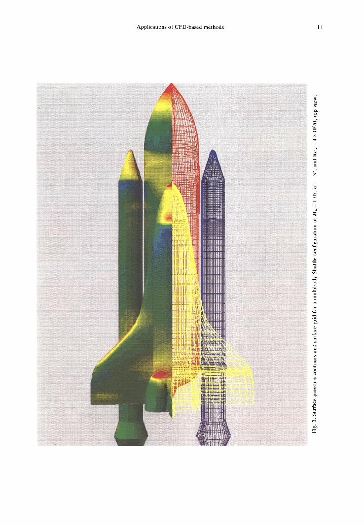
In order to illustrate the present status of CFD, the modeling of the viscous, near sonic flow over the en- tire Shuttle mated configuration is shown in Fig. 3, and a sample correlation of Orbiter surface pressures on the side of the fuselage between computation and experimental data is shown in Fig. 4. Reference 13 provides many more results for the Shuttle problem.

CFD, which has been taxing the vector supercomputers, such as the CRAY-YMP with eight processors, to their limits (both memory and execution speed), is starting to embark on algorithm designs (both software and hardware) for massively parallel processing. 14

COMPUTATIONAL AEROELASTICITY

In the spirit of developing a computational environment to encompass many disciplines as shown in Fig. 1, a preliminary multidisciplinary computation involving coupling of CFD codes, aeroelastic structural response, and active control laws is set up as outlined in Fig. 5. The CFD component in this coupling process is providing the aerodynamic load acting on a flexible structure and, depending on the physics being modeled, one can employ any one of the hierarchy of CFD tools (full potential, Euler, Navier-Stokes, . . .).

Aeroelastic model

The aeroelastic model is based on the generalized modal approach. In the physical space, the structural equation is written as

[m]2+,[c]2+ [k]z = {f), (8)

6-

oa

Fig

. 3.

Sur

face

pre

ssur

e co

ntou

rs a

nd s

urfa

ce g

rid

for

a m

ult

ibod

y Sh

uttl

e co

nfig

urat

ion

at M

~ =

1.05

, ~

= -3

°,

and

Rex

= 4

x 1

0o/f

t, t

op v

iew

.


0.80 I I I I + ' 9 0 0

0.32

-0 .16

I

- 0.54

-1 .12 o ~ - 0 0 /

- 1.60 ~ I I I 550 810 1070 1330 1590 1850

x (INCHES) Fig. 4. Comparison of pressure coefficient from computation ( ) with experimental data (©) at a side fuselage loca-

tion. M~ = 1.05, ~ = - 3 °, Re~ = 4 x 106/ft.

where m, c, k, and f represent the mass, damping, stiffness, and force, respectively. Corresponding to each natural frequency toi [eigenvalues of Eq. (8)], there exists an eigenvector (Di which represents the amplitude of deflection of the various points of the system. For the first n modes of natural frequency, one can compute the n left and right eigenvectors forming the generalized mode shapes. Using the generalized mode shape, one can rewrite Eq. (8) as

M{gl}+[C]{q)+[K]{q} = {F}, (9)

where M, C, and K are generalized mass, damping, and stiffness matrices and {F) is the generalized force. These are defined by M = +rm+, K= +Tk+, C=4)rc4~, F=+rf, and z=+q, where q is the generalized deflection.

The aeroelastic coupling can be performed under any of the following modes: (1) static flexible, (2) dynamic flexible, and (3) dynamic flexible with active feedback control law. The implementation details, including the dynamic grid update procedure

GEOMETRY AND GRID SETUP I

GEOMETRY AND GRID UPDATE ]

* CFD I (LOADS)

I STRUCTURAL I RESPONSE

STRUCTURAL OPTIMIZATION

• CONTROL LAW • CONTROL SETTING

Fig. 5. Coupling of aerodynamics, aeroelasticity, and controls.

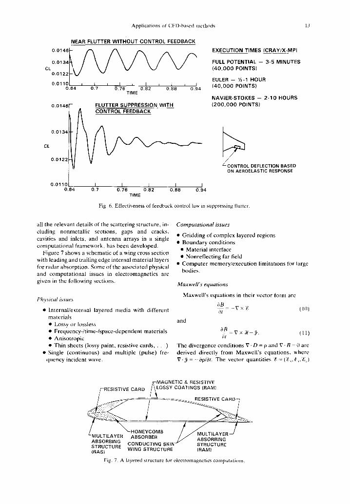
and appropriate feedback control laws for flutter suppression, are given in Refs 15 and 16. Figure 6 illustrates the effectiveness of a feedback control law in damping out flutter by showing the time history of lift variation due to aeroelastic motion.

COMPUTATIONAL ELECTROMAGNETICS

As mentioned earlier, the development of modern aerospace vehicle concepts increasingly requires coupled optimization studies involving fluid dynamics, structures, propulsion, controls, and electromagnetics [radar cross section (RCS)]. In the process of developing a muitidisciplinary computational environment, one of the goals is to provide a unified numerical treatment for the many different mathematical equations representing different physics. For example, just like fluid dynamics problems are modeled by Navier-Stokes equations, the electromagnetics discipline is modeled by Maxwell's equations. Though they represent a totally different physics, there is a lot of commonality between the two equations at the differential equation level. The objective here is to employ the mathematic rigor and algorithmic elegance of CFD to solve problems in CEM and be able to eventually perform coupled CFD/CEM optimization studies under a unified algorithmic framework of Fig. 1.

The ability to predict radar return from complex structures with layered material media over a wide frequency range (100 MHz-20 GHz) is a critical technology requirement for the development of stealth aerospace configurations. Traditionally, RCS calculations have employed one of two methods: high frequency asymptotics, which treats scattering and diffraction as local phenomena; or solution of an integral equation for radiating sources on (or inside) the scattering body, which couples all parts of the body through a multiple scattering process. A third approach is the direct integration of the differential form of Maxwell's equations in time.

The time-domain Maxwell equations represent a more general form than do the frequency-domain vector Helmholtz equations, which are usually employed in solving scattering problems. A time- domain approach can, for instance, handle continuous waves (single frequency, harmonic) as well as a single pulse (broadband frequency) transient response. Frequency-domain-based methods usually provide the RCS response for all angles of incidence at a single frequency, while time-domain-based methods provide solutions for many frequencies from a single transient calculation. Also, in a time- domain approach, one can consider time-varying material properties for treatment of active surfaces. By using special methods, the time-domain transient solutions can be processed to provide the frequency-domain response.

A general time-domain approach based on proven CFD-based numerical techniques which can capture


N E A R F L U T T E R W I T H O U T C O N T R O L F E E D B A C K

0.0134

C L o . o 1 2 2 r ~ /

0 . 0 1 1 0 L I I I I t I , I , I 0.64 0.7 0.76 0.82 0.88 0.94

TIME

0.0146

0 . 0 1 3 4

CL

0 . 0 1 2 2

- F L U T T E R S U P P R E S S I O N WITH

0 . 0 1 1 0 i I I I I J 0 . 6 4 '0.7 0 . 7 6 0 . 8 2 0 . 8 8 0 . 9 4

TIME

E X E C U T I O N T I M E S ( C R A Y / X - M P )

FULL POTENTIAL -- 3-5 MINUTES ( 4 0 , 0 0 0 POINTS)

E U L E R - ½ - 1 H O U R ( 4 0 , 0 0 0 POINTS)

N A V I E R - S T O K E S - - 2 - 1 0 H O U R S ( 2 0 0 , 0 0 0 P O I N T S )

Z C O N T R O L DEFLECTION BASED ON AEROELASTIC RESPONSE

Fig. 6. Effectiveness of feedback control law in suppressing flutter.

all the relevant details of the scattering structure, including nonmetall ic sections, gaps and cracks, cavities and inlets, and antenna arrays in a single computat ional f ramework, has been developed.

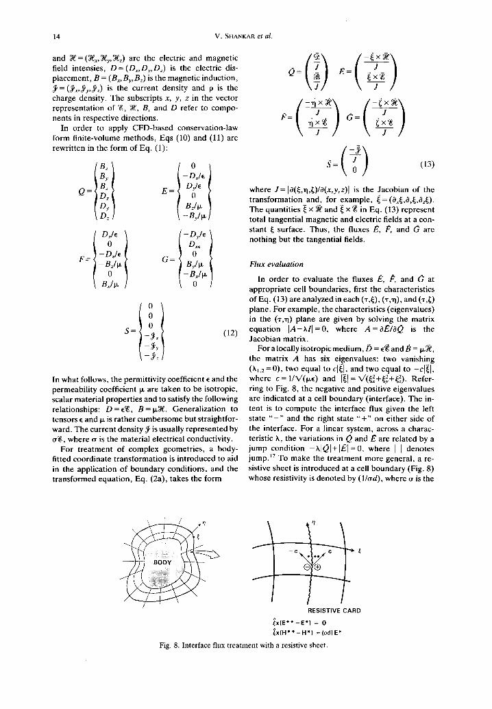
Figure 7 shows a schematic of a wing cross section with leading and trailing edge internal material layers for radar absorption. Some of the associated physical and computat ional issues in electromagnetics are given in the following sections.

Physical issues

• Internal/external layered media with different materials • Lossy or lossless • Frequency-/ t ime-/space-dependent materials • Anisotropic • Thin sheets (Iossy paint, resistive cards . . . . )

• Single (continuous) and multiple (pulse) frequency incident wave.

Computational issues

• Gridding of complex layered regions • Boundary conditions

• Material interface • Nonreflect ing far field

• Compute r memory/execut ion limitations for large bodies.

Maxwell's equations

Maxwelrs equat ions in their vector form are

OB - - V x ~

at

and

(m)

~B -V x ~-~. (11)

0t

The divergence conditions V. D = p and V. B = 0 are derived directly from Maxwelrs equations, v,'here V - ~ = - a p / a t . The vector quantities ~#~ = ( '~, ~;,.,'~)

RES,ST,V CARD

::iii:!!!:ii:f : ~ / - ~_

COMB ULTILAYER ABSORBER / / / AI3SOtXnc:nnm~J~

S TI~UC'TURE CONDUCTING SKIN~ STRUCTURE WING STRUCTURE (RAM) (RAS)

Fig. 7. A layered structure for electromagnetics computations.


and ~' = (~ ,~y,~ '~) are the electric and magnetic field intensies, D = (Dx, Dy, Dz) is the electric dis- placement, B = (Bx, By, B~) is the magnetic induction,

= ()~,)y,¢~) is the current density and p is the charge density. The subscripts x, y, z in the vector representation of %, ~£, B, and D refer to components in respective directions.

In order to apply CFD-based conservation-law form finite-volume methods, Eqs (10) and (11) are rewritten in the form of Eq. (1):

Q= t By [ -- D J•

D~ E= Dy [ Bz/Ix Dz ~ - By/Ix

F=

D~

- D ~ I e

-B/Ix

Bx/IX

G= -Dy/EDo~,: 1

By~Ix

-"0 J~ )

S= (12)

In what follows, the permittivity coefficient • and the permeability coefficient Ix are taken to be isotropic, scalar material properties and to satisfy the following relationships: D=•%, B= Ix~'. Generalization to tensors ~ and Ix is rather cumbersome but straightfor- ward. The current density ) is usually represented by tr%, where ~ is the material electrical conductivity.

For treatment of complex geometries, a body- fitted coordinate transformation is introduced to aid in the application of boundary conditions, and the transformed equation, Eq. (2a), takes the form

(13)

where J = Io(E,~l,K)/O(x,y,z)l is the Jacobian of the transformation and, for example, ~= (Ox~,Oy~,O,O. The quantities t~ x ~' and ~ x % in Eq. (13) represent total tangential magnetic and electric fields at a con- stant 1~ surface. Thus, the fluxes E, F, and (3 are nothing but the tangential fields.

Flux evaluation In order to evaluate the fluxes /~, /e, and (~ at

appropriate cell boundaries, first the characteristics of Eq. (13) are analyzed in each ('r,l~), (x,-q), and (¢,~) plane. For example, the characteristics (eigenvalues) in the ('r,-q) plane are given by solving the matrix equation I A - k l I = 0 , where A=OF,/O0_ is the Jacobian matrix.

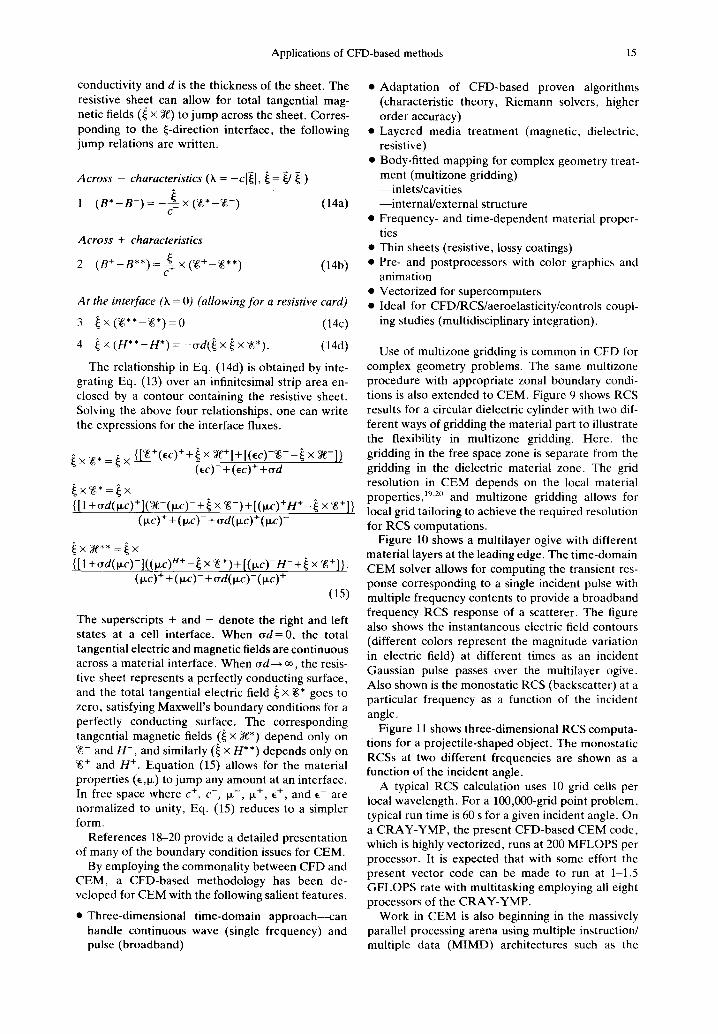
For a locally isotropic medium, b = •~ and B = Ix~, the matrix A has six eigenvalues: two vanishing (h,.2=0), two equal to cl l, and two equal to -c[~ l, where c= 1/X/(IX~) and ]~1 = X/(~+~yZ+~2) • Refer- ring to Fig. 8, the negative and positive eigenvalues are indicated at a cell boundary (interface). The in- tent is to compute the interface flux given the left state . . . . . and the right state "+" on either side of the interface. For a linear system, across a characteristic h, the variations in O and/~ are related by a jump condition -~101+1~1=0, where II denotes jump. '7 To make the treatment more general, a resistive sheet is introduced at a cell boundary (Fig. 8) whose resistivity is denoted by (l&rd), where tr is the

f

RESISTIVE C A R D ^ , ~ x ( E * * - E * ) = 0

i x ( H * * - H * ) =(odl E*

Fig. 8. Interface flux treatment with a resistive sheet.


conductivity and d is the thickness of the sheet. The resistive sheet can allow for total tangential magnetic fields (~ x I~) to jump across the sheet. Corres- ponding to the ~-direction interface, the following jump relations are written.

Across - characteristics (h = -c l~ l , ¢ = ~/1~1)

1 ( B * - B - ) = -=~_ x (%*-%-) (14a)

Across + characteristics

( B + - B **) := c~% x (%+-%**) 2 (14b)

A t the interface' (X = O) (allowing for a resistive card)

3 ~ x (%**-%*)=0 (14c)

4 ~ x ( H * * - t t * ) = -~rd(~ x ~ x %*). (140)

The relationship in Eq. (14d) is obtained by integrating Eq. (13) over an infinitesimal strip area en- closed by a contour containing the resistive sheet. Solving the above four relationships, one can write the expression,; for the interface fluxes.

,~ x ~* = ~ x {[~"( '~c)++~ x ~ + ] + [ ( ~ c ) - ~ - - ~ x ~ -1 } (~c)-+(~c)++~d

t~ × ~,~ * =~x { [ I +o-d( ixc)+] (~-(~c)- + ~; x ~ - )+ [ ( . . c )+H+- ,~ x ~+1)

(o.c) + + (o.c)- + (rd(ixc) +(o.c)-

~×~**=~x ([1 +(rd(Ixc)-]((Ixc)H+--~ x %+) + [(la.c)-H- +,~ x %+]}.

(o.c) + +(o.c)- +,~d(~c)-(o.c) + (15)

The superscripts + and - denote the right and left states at a cell interface. When ~rd=0, the total tangential electric and magnetic fields are continuous across a materJial interface. When ~rd~ ~ , the resistive sheet represents a perfectly conducting surface, and the total tangential electric field ~ × %* goes to zero, satisfying Maxwell's boundary conditions for a perfectly conducting surface. The corresponding tangential magnetic fields (~ × ~*) depend only on %- and H - , and similarly (~ × H**) depends only on %+ and H +. E, quation (15) allows for the material properties (e,p.) to jump any amount at an interface. In free space where c +, c , tx , ix +, e+, and e- are normalized to unity, Eq. (15) reduces to a simpler form.

References 18-20 provide a detailed presentation of many of the boundary condition issues for CEM.

By employing the commonality between CFD and CEM, a CFD-based methodology has been developed for CEM with the following salient features.

• Three-dimensional time-domain approach---can handle continuous wave (single frequency) and pulse (broadband)

• Adaptat ion of CFD-based proven algorithms (characteristic theory, Riemann solvers, higher order accuracy)

• Layered media treatment (magnetic, dielectric, resistive)

• Body-fitted mapping for complex geometry treatment (multizone gridding) --inlets/cavities -- internal /external structure

• Frequency- and time-dependent material properties

• Thin sheets (resistive, lossy coatings) • Pre- and postprocessors with color graphics and

animation • Vectorized for supercomputers • Ideal for CFD/RCS/aeroelasticity/controls coupl-

ing studies (multidisciplinary integration).

Use of multizone gridding is common in CFD for complex geometry problems. The same multizone procedure with appropriate zonal boundary conditions is also extended to CEM. Figure 9 shows RCS results for a circular dielectric cylinder with two different ways of gridding the material part to illustrate the flexibility in multizone gridding. Here. the gridding in the free space zone is separate from the gridding in the dielectric material zone. The grid resolution in CEM depends on the local material properties, ~9'2° and multizone gridding allows for local grid tailoring to achieve the required resolution for RCS computations.

Figure 10 shows a multilayer ogive with different material layers at the leading edge. The time-domain CEM solver allows for computing the transient response corresponding to a single incident pulse with multiple frequency contents to provide a broadband frequency RCS response of a scatterer. The ligure also shows the instantaneous electric field contours (different colors represent the magnitude variation in electric field) at different times as an incident Gaussian pulse passes over the multilayer ogive. Also shown is the monostatic RCS (backscatter) at a particular frequency as a function of the incident angle.

Figure 11 shows three-dimensional RCS computations for a projectile-shaped object. The monostatic RCSs at two different frequencies are shown as a function of the incident angle.

A typical RCS calculation uses 10 grid cells per local wavelength. For a 100,000-grid point problem, typical run time is 60 s for a given incident angle. On a CRAY-YMP, the present CFD-based CEM code, which is highly vectorized, runs at 200 MFLOPS per processor. It is expected that with some effort the present vector code can be made to run at 1-1.5 GFLOPS rate with multitasking employing all eight processors of the CRAY-YMP.

Work in CEM is also beginning in the massively parallel processing arena using multiple instruction/ multiple data (MIMD) architectures such as the

,o] I

0q

-10

-20

RC

S

o E

XA

~

--C

OM

PU

TA

~O

N

~A

o -,~

u,

PO

LA

R

GR

ID

~ -4

0

ili

..............

.. _,o -6

0

-70

0

!! FI

ELD

CO

NTO

UR

S

~__1

1 ~'

''" ~' ;i. ....

... "

i~

y NE

AR RE

CTAN

GUL

AR

Fig.

9.

Fle

xibi

lity

in

mul

tizo

ne g

ridd

ing.

Cas

e of

a c

ircu

lar

diel

ectr

ic o

bjec

t.

:.;;

- .-

~,,2

.56

.; ~,

/°

45

90

1

35

1

80

2

25

2

70

3

15

3

60

0 (V

IEW

ING

AN

GLE

)

< Z

GE

OM

ETR

Y

15- 5

> < < -5

-15

"O

-25

-35

0

GR

ID

SC

§180

2

| I

I I

I 0

0

.A

- Q

O

"

g_

o

nDO

_

| O

GIV

E (

TEl

I --

MO

M

BA

CK

SC

ATT

ER

I I

I I

I 30

60

90

12

0 15

0 18

0 A

NG

LE (

DEG

)

Fig.

10.

Rad

ar c

ross

sec

tion

for

a m

ulti

laye

red

ogiv

e.

;TA

NTA

NE

OU

S F

IELD

CO

NTO

UR

S

> w

5'

==

-tl

O"

=-

C;

o , ? v ?

oll>X 0

T

g

5

N

- I

N RCS (DBSM)

k " " "

~-~

# ,

m

I "

c,}

m

0

m I'- I'I"I 0 -,I i

0 "1"I m

m I-" o 0 0 Z .-I 0

rio

.L "~ ., .:,~,

C'-",~Q~'L~ .~,,- \, 3, <..~

[u #a ovA~v~ A ~L


L.AYERED AIRFOIL DIELECTRIC CYLINDER

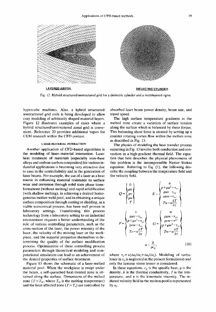
Fig. 12. Hybrid structured/unstructured grid for a dielectric cylinder and a multilayered ogive.

hypercube machines. Also, a hybrid structured/ unstructured grid code is being developed to allow easy modeling of arbitrarily shaped material layers. Figure 12 illustrates examples of cases where a hybrid structured/unstructured zonal grid is conve- nient. Reference 20 provides additional topics for CEM research within the CFD context.

LASER-MATERIAL INTERACTION

Another application of CFD-based algorithms is the modeling of laser-material interaction. Laser heat treatment of materials (especially iron-base alloys and carbon-carbon composites) for various industrial applications is becoming very attractive due to ease in the controllability and in the generation of laser beams. For example, the use of a laser as a heat source in enhancing material resistance to surface wear and corrosion through solid state phase trans- formations (without melting) and rapid solidification (with shallow melting), in achieving a desired homo- geneous molten weld pool, and in obtaining a unique surface composition through coating or cladding, as a viable economical process, has been well proven in laboratory settings. Transitioning this process technology from a laboratory setting to an industrial environment requires a better understanding of the rote of various controlling parameters, such as the cross-section of the laser, the power intensity of the laser, the velocity of the moving laser or the workpiece, and the material properties themselves in de- termining the quality of the surface modification process. Optimization of these controlling process parameters through theoretical modeling and computational simulation can lead to an achievement of the desired properties of surface treatment.

Figure 13 shows the schematic of a laser-melted material pool. When the workpiece is swept under the beam, a self-quenched heat-treated zone is obtained along the surface. Dimensions of the melted zone ( T > Tin, where Tm is the melting temperature) and the heat-affected zone ( T > T¢) are controlled by

absorbed laser beam power density, beam size, and travel speed.

The high surface temperature gradients in the melted zone create a variation of surface tension along the surface which is balanced by shear forces. This balancing shear force is created by setting up a counter rotating vortex flow within the molten zone as described in Fig. 13.

The physics of modeling the heat transfer process occurring in Fig. 13 involve both conduction and convection in a high-gradient thermal field. The equation that best describes the physical phenomena of this problem is the incompressible Navier-Stokes equation. Referring to Eq. (1), the following describe the coupling between the temperature field and the velocity field.

pu Q = pv

P + P u u - Txz E = ~ puv - ' r xy

I p t lw_,rx z

F=

v

pUV--Txy p+pv2-- 'ryy

pVW--Ty z

Tv - e~ ~y

G=

w

puw--'rxz ppw- -T yz

p+pw2-- ' rzz

T w - e ~ z

a - k (16) p ~ '

where %=v(Oui/Oxj+OuJOxi). Modeling of turbulence in % is neglected in the present formulation and only the laminar stress tensor is considered.

In these equations, cp is the specific heat, p is the density, k is the thermal conductivity, T is the lem- perature, and v is the kinematic viscosity. The induced velocity field in the molten pool is represented by uj.


MOVIN( LASER BEAM

~'-MZ (T > Tin)

~ - H A Z T > T c

MZ - MELTED ZONE

HAZ - HEAT AFFECTED ZONE T c - PHASE TRANSFORMATION TEMP.

T m - MELTING TEMP.

CROSS SECTION

Q LONGITUDINAL VIEW

LASER

. o

TOP VIEW - - o v N / THREE-DIMENSIONAL VORTEX FLOW

- ' - ~ U I;URFACE VELOCITY VECTORS -

Fig. 13. Surface tension induced convective heat t ransfer in laser-material interaction.

In the unmelted region of the material where the heat transfer process is purely due to conduction (temperatures below melting), only the energy equation needs to be solved for temperature. 2'

On the outer surface of the molten pool, the force balance equations are

Ou ,OT

Ov ,OT I~z = cr ~yy, (17)

where cr' is the rate of change of surface tension (N m -~ kg -~) with temperature and p. is the coefficient of viscosity of the molten pool (Ns m-2).

At the liquid-solid interface u = v = w = 0 and T= T,.. More details on the boundary condition can be found in Ref. 22. The computational method employs an implicit triple approximate factorization scheme to solve the energy equation in terms of temperature and an explicit treatment for the three momentum equations and the continuity equation. 2z The pressure field is updated at each time level using a Poisson solver to satisfy the continuity equation.

Laser results

A sample result for a rectangular workpiece undergoing melting is presented.

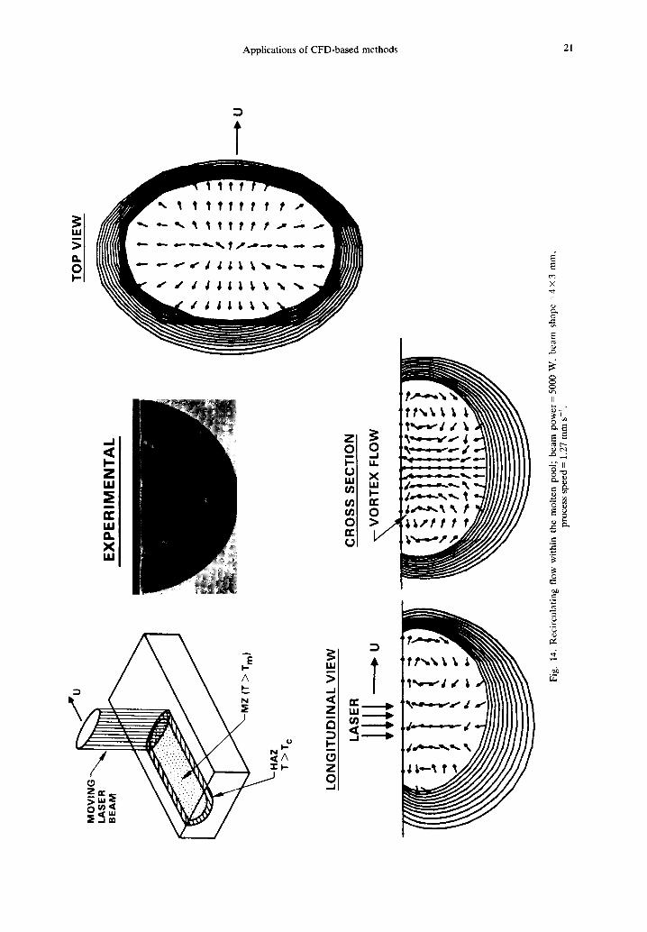
Figure 14 shows results for a typical case (5000 W laser, 4 x 3 mm laser cross ~ection, 1.26 mm s- ' beam

travel speed). A point in the workpiece is considered heat-affected if that point experiences temperatures above 750°C and the melt zone corresponds to temperatures > 1500°C. At a given instance of time (laser beam around the halfway length of the workpiece), the instantaneous temperature distribution, melt zone shape, and the three-dimensional vortex mixing material flow are as shown in Fig. 14. The cross sectional view, longitudinal view (plane of symmetry), and the top view of the melted zone clearly reveal the convection process induced by the surface tension driven flow. Pure conduction treatment of this heat transfer problem (no convection model, i.e. surface tension gradients set to zero) results in temperature levels not comparable with experimental observations. The computational procedure of the present study incorporating the surface tension driven convective heat transfer process pro- duces melt zone and heat-affected zone shapes very similar to those of experimental data. More results are presented in Ref. 22.

Application of this work to study problems of deep welding (solute redistribution, microstructure of the heat-affected zone, and residual stress state) and characterization of the surface ripples are some of the ongoing projects.

CONCLUSIONS

The state of the art of CFD has taken rapid strides in recent years with the development and application

MO

VIN

G~

~

U

LAS

ER

~-

IIIItl

II]T

~I _

~ ,~

~

'MZ

(T

>

Tm

_.

HA

z

)

T >

T c

EX

PE

RIM

EN

TA

L

LON

GIT

UD

INA

L V

IEW

LAS

ER

C

RO

SS

SE

CT

ION

~ --

---~

U

VO

RT

EX

FLO

W

TOP

VIE

W

~-U

>

J.

Q

O"

e~

O

Fig.

14.

Rec

ircu

latin

g fl

ow w

ithin

the

mol

ten

pool

; be

am p

ower

=50

00 W

, be

am s

hape

=4

z 3

mm

, pr

oces

s sp

eed

= 1

.27

mm

s -1.


of unified, robust , and efficient methods . The ad- vances in C F D are also beg inn ing to make a posi t ive impact on o the r areas of ma themat i ca l science, leading to the e m e r g e n c e of the concep t of " C o m p u t a - t ional Science ." In this new spirit , this pape r has p re sen ted a unif icat ion of a lgor i thms and the i r appli- cat ion to fluid dynamics , aeroelast ic i ty , e lectro- magnet ics , and mater ia l charac ter iza t ion . The goal is to be able to achieve in tegra t ion of mult idiscipl inary technologies as ske tched in Fig. 1.

REFERENCES

1. S. R. Chakravarthy and S. Osher, "Computing with high-resolution upwind schemes for hyperbolic equations," Lectures in Applied Mathematics 22, 57-86 (1985).

2. S. R. Chakravarthy, "Development of upwind schemes for the Euler equations," NASA CR-4043, January 1987.

3. V. Shankar, "A unified full potential scheme for subsonic, transonic, and supersonic flows," A I A A Paper No. 85-1643, A I A A 18th Fluid Dynamics, Plasma- dynamics, and Lasers Conference, Cincinnati, OH, 16- 18 July 1985.

4. V. Shankar, K.-Y. Szema and S. Osher, "A conserva- tive type-dependent full potential method for the treatment of supersonic flows with embedded subsonic regions," AIAA Journal 23, 41-48 (1985).

5. V. Shankar, H. lde, J. Gorski and S. Osher, "A fast, time-accurate unsteady full potential scheme," AIAA Journal 25, 230-238 (1987).

6. V. Shankar and H. Ide, "'Unsteady full potential computations for complex configurations," AIAA Paper No. 87-0110, AIAA 25th Aerospace Sciences Meeting, Reno, NV, January 1987.

7. K.-Y. Szema, S. R. Chakravarthy and H. Dresser, "Multizone Euler marching technique for flows over multibody configurations," AIAA Paper No. 87-0592, January 1987, and AIAA Paper No. 88-0276, January 1988.

8. S. R. Chakravarthy, K.-Y. Szema and J. W. Haney, "Unified nose-to-tail computational methods for hypersonic vehicle applications," AIAA Paper No. 88- 2564, June 1988.

9. U. Goldberg and S. Chakravarthy, "Separated flow predictions using a hybrid k-L/backflow model," A1AA Paper No. 89-0566, 27th Aerospace Sciences Meeting, Reno, NV, 9-12 January 1989.

10. S. palaniswamy, S. R. Chakravarthy and D. K. Ota, "Finite rate chemistry for USA-series codes: formula-

tion and applications," AIAA Paper No. 89-0200, 27th Aerospace Sciences Meeting, Reno, NV, 9-12 January 1989.

1 I. J. F. Thompson, Z. U. A. Warsi andC. Wayne Martin, Numerical Grid Generation--Foundations and Appli- cations, North-Holland, Amsterdam, 1985.

12. C. Gumbert, R. L6hner, P. Parikh and S. Pirzadeh, "A package for unstructured grid generation and finite element flow solvers," AIAA Paper No. 89-2175-CP, 1989.

13. C.-L. Chen, S. Ramakrishnan, K.-Y. Szema, H. S. Dresser and K. Rajagopal, "'Multizonal Navier-Stokes solutions for the multibody Space Shuttle configuration," A1AA Paper No. 90-0434, 28th Aerospace Sciences Meeting, Reno, NV, 8-11 January 1990.

14. D. K. Wilde, "A custom processor for use in a parallel computer system," IEEE 1989 Custom Integrated Cir- cuits Conference, June 1989, pp. 10.5.1-10.5.5.

15. V. Shankar and H. Ide, "'Unsteady aeroelastic computations for flexible configurations at transonic and supersonic speeds," lUTAM Symposium TRANS- SONICUM Ill, DFVLR-AVA, G6ttingen, Germany, 24-27 May 1988, Springer, Berlin, pp. 465-478.

16. D. Ominsky and H. lde, "An effective flutter control method using fast, time-accurate CFD codes," AIAA Paper No. 89-3468, AIAA Guidance, Navigation, and Control Conference, Boston, MA, 14-16 August 1989.

17. P. Lax, "'Hyperbolic systems of conservation laws and the mathematical theory of shock waves," Lecture Series in Applied Mathematics, Vol. 11, SIAM, Philadelphia, PA, 1973.

18. V. Shankar, W. F. Hall and A. H. Mohammadian, "A time-domain differential solver for electromagnetic scattering problems,'" Proceedings of the IEEE 77, 709- 721 (1989).

19. V. Shankar, W. F. Hall and A. Mohammadian, "A CFD-based finite-volume procedure for computational electromagnetics--interdisciplinary applications of CFD methods," AIAA Paper No. 89-1987, AIAA 9th Computational Fluid Dynamics Conference, Buffalo, NY, 13-15 June 1989.

20. V. Shankar, A. H. Mohammadian and W. F. Hall, "'A time-domain, finite-volume treatment for the Maxwell equations," Electromagnetics 10 (1990) (to appear).

21. V. Shankar and D. Gnanamuthu, "'Computational simulation of laser heat processing of materials," AIAA Paper No. 85-0390, 23rd Aerospace Sciences Meeting, Reno, NV, 14-17 January 1985. Also presented at the International Symposium on Computa- tional Fluid Dynamics--Tokyo, Kenchiku-kaikan, Tokyo, 9-12 September 1985.

22. V. Shankar and D. Gnanamuthu, "Computational simulation of heat transfer in laser melted material flow," AIAA Paper No. 86-0461, 24th Aerospace Sci- ences Meeting, Reno, NV, 6-9 January 1986.

Documents

Applications of Computational Fluid Dynamics-based methods to problems in computational science