Embed Size (px)
Citation preview

4020
ISSN 2286-4822
www.euacademic.org
EUROPEAN ACADEMIC RESEARCH
Vol. IV, Issue 4/ July 2016
Impact Factor: 3.4546 (UIF)
DRJI Value: 5.9 (B+)
Applications of biostatistics in food science –
Review
ANWAR NOMAN1
State key Laboratory of Food Science and Technology
& School of Food Science and Technology
Jiangnan University, P. R. China
Department of Agricultural Engineering, Faculty of Agriculture
University of Sana`a, Sana`a, Yemen
AMMAR ALFARGA
State key Laboratory of Food Science and Technology
& School of Food Science and Technology
Jiangnan University, P.R.China
SHERIF M. ABED
State key Laboratory of Food Science and Technology
& School of Food Science and Technology
Jiangnan University, P.R.China
Food and dairy sciences and technology department
Faculty of Environmental Agricultural Science
El Arish University, Egypt
AMER ALI MAHDI
State key Laboratory of Food Science and Technology
& School of Food Science and Technology
Jiangnan University, P.R.China
Department of Food Science and Technology, Faculty of Agriculture
Sana‘a University, Sana‘a, Yemen
XIA WENSHUI
State key Laboratory of Food Science and Technology
& School of Food Science and Technology
Jiangnan University, P.R.China
Abstract:
Statistical methods are important aids to detect trends, explore
relationships and draw conclusions from experimental data. The aim
1 Corresponding author: [email protected]

Anwar Noman, Ammar Alfarga, Sherif M. Abed, Amer Ali Mahdi, Xia Wenshui-
Applications of biostatistics in food science – Review
EUROPEAN ACADEMIC RESEARCH - Vol. IV, Issue 4 / July 2016
4021
of this paper is to present some of statistical techniques and to
highlight their uses based on practical examples in Food Science and
Technology like Standard Deviation, Normality, ANOVA, Correlation
analysis and other statistical methods.
Key words: Biostatistics, Statistical methods, Standard Deviation,
Normality, ANOVA, Correlation analysis.
INTRODUCTION
Statistical analysis, which is defined as the process of making
scientific inferences from data that contain variability, has
historically played an integral role in advancing nutritional
sciences. This tool has gained an increasingly important role in
the systems biology era to analyze large, complex data sets
generated from genomics, proteomics and metabolomics
studies[1-2 ].Particularly, analyses of data from the reverse
transcriptase-polymerase chain reaction (RT-PCR) as well as
microarray, proteomics and other bioinformatics studies
requires statistical models to account for various sources of
variations[3-4 ].Appropriate statistical methods can minimize
systemic errors, optimize data analysis, and identify which
genes are differentially expressed in the face of substantial
biological and technical variations[5-4].Statistics is essentially
a branch of mathematics applied to analysis of data. In Food
Science, statistical procedures are required in the planning,
analysis and interpretation of experimental work. Such work
may include surveys of the chemical, physical, sensory and
microbiological composition of food and beverages during
development and manufacture, including changes to these
properties as a consequence of process optimization. Currently,
many software packages are available that facilitate statistical
analysis of data; when used properly they provide a valuable
tool to enable different types of statistical and mathematical
analyses to be done rapidly. Such software packages take

Anwar Noman, Ammar Alfarga, Sherif M. Abed, Amer Ali Mahdi, Xia Wenshui-
Applications of biostatistics in food science – Review
EUROPEAN ACADEMIC RESEARCH - Vol. IV, Issue 4 / July 2016
4022
seconds to generate linear/non-linear models, draw graphs or
resolve complex numerical algorithms that used to take a
considerable amount of time using manual procedures.
The importance of proper application of statistics in
Food Research cannot be ignored; it is essential if one is to
understand data and make decisions that take account of the
statistical variability of measurement and process control
systems, summarize experimental.
CONCEPTS OF STATISTICS APPLIED IN FOOD
SCIENCE
Use of the correct statistical tools is essential since the
researcher needs to extract as much information as possible
from experimental results. When work is published in a journal
sufficient detail must be provided to permit the reader to
understand fully the aims and outcome of the research and,
should it be appropriate.
The total variance of a specific sampling plan (TV, also
indicated as ‖Total error‖), may be expressed by using statistic
variance as a measure of variability and may be described as
the sum of sampling variance (SV), sample preparation
variance (SPV), and analytical variance (AV) as follows:
TV=SV+SPV+AV.
The reported analysis of results is often restricted to descriptive
statistics (mean, median, minimum, maximum values,
standard deviation and/or coefficient of variation). These, and
other statistical tests such as correlation, regression, and
comparison of mean values, are often based on the slavish use
of ‗statistical packages‘ that may, or may not, be appropriate for
the purpose.
All of these considerations should be addressed prior to
setting up an experimental plan and all are generally within
the control of the researcher. Sometimes experimental results

Anwar Noman, Ammar Alfarga, Sherif M. Abed, Amer Ali Mahdi, Xia Wenshui-
Applications of biostatistics in food science – Review
EUROPEAN ACADEMIC RESEARCH - Vol. IV, Issue 4 / July 2016
4023
may fall outside the limits of an analytical method; for instance,
the level of an analyte in a sample may be below the lowest
limit or, more rarely, above the highest limit of detection or
quantification of a method. Such results are referred to as left-
or right-censored values, respectively. How should such results
be handled? This is a subject much under discussion in many
fields, including (food) chemistry, microbiology and toxicology
and several questions still need to be addressed with respect to
the suitability of the procedure used to handle censored [6-7].
A procedure, known as the Tobit regression, for
evaluation of censored data in food microbiology has been
described by [8].— the concepts are equally applicable in other
areas of Food Science.
Two characteristics of data sets must be considered prior
to the application of any inferential tests:
1. Do the data conform to the principles of ‗normality‘,
i.e. to a ‗normal‘ distribution (ND)
2. Do the data satisfy an assumption of
homoscedasticity, i.e. uniformity of variance.
What do we mean by a ‗normal‘ distribution (ND). A population
ND can be described as a bell-shaped curve (Fig. 1) under which
approximately 95% of values lie within the range mean (μ) ± 2
standard deviations (σ) and approximately 99% lie within the
range μ ± 3σ. The standard deviation is a measure of the
dispersion of values around the mean value and is determined
as the square root of the variance, i.e.σ ¼ = σ2. The mean value
(x) and standard deviation (s) of a set of data obtained by
analysis of random samples provide estimates of the population
statistics.
If a number of random samples from a ‗lot‘ or ‗batch‘ of
food, or indeed of other test matrix, is analyzed for some
particular attribute (e.g. sugar content, acidity, pH level) it
would be unrealistic to assume that the analytical results will
be absolutely identical between the different samples, or even

Anwar Noman, Ammar Alfarga, Sherif M. Abed, Amer Ali Mahdi, Xia Wenshui-
Applications of biostatistics in food science – Review
EUROPEAN ACADEMIC RESEARCH - Vol. IV, Issue 4 / July 2016
4024
between subsamples of the same product. The reasons relate to
the measurement uncertainty of the analytical method used for
the test and the intrinsic variation in composition that occurs
both within and between samples.
We would therefore expect to obtain a range of values
from the analyses. If only a few samples are analyzed, the
results may appear to be randomly distributed between the
lowest and highest levels (Fig. 2A); but if we were able to
examine at least 20 samples, we would expect to obtain a
distribution of results that conform reasonably well to a ND
(Fig. 2B) with an even spread of results on either side of the
mean value. However, in some cases, the distribution will not
be ‗normal‘ and may show considerable skewness (Fig. 2C) —
such results would be expected, for instance, in the case of
microbiological colony counts.
Fig.1. A population normal distribution (ND) curve showing that
approximately 95.45% of all results lie within ±2 standard deviations (s) of the
mean and 99.73% lie within ±3s. Modified from [9]
STATISTICAL MODELING AND DATA ANALYSIS
Depending on study design and the type of response variables,
data will be analyzed with use of different statistical models to
reflect the data structure and potential correlation between
observations. Categorical response variables are usually
Anwar Noman, Ammar Alfarga, Sherif M. Abed, Amer Ali Mahdi, Xia Wenshui-
Applications of biostatistics in food science – Review
EUROPEAN ACADEMIC RESEARCH - Vol. IV, Issue 4 / July 2016
4025
analyzed using contingency tables, logistic regressions, or
generalized estimation equations (GEE) models. The
contingency tables can also be used to test the homogeneity of
distributions for categorical response or explanatory variables.
In contrast, continuous response variables are analyzed using
the t test, analysis of variance (ANOVA), correlation, and
regression [10].Statistical modeling is the data processing step
to sort out information from a study. This can be achieved by
building a quantitative relationship between the outcome or
response variables and the explanatory or independent
variables through a mathematical model or equation that
characterizes the dependence of the former on the latter. In
modeling response variables, their correlations should receive
special attention, because the responses (e.g., body weights of
the same subject at different time points) are highly correlated
and thus the correlation structure should be incorporated into
data analysis. Therefore, longitudinal studies should be
carefully analyzed for the following reasons: First, subjects are
monitored with multiple observations at different time points.
Second, the correlation structure between observations affects
estimation accuracy and subsequent inference [11].
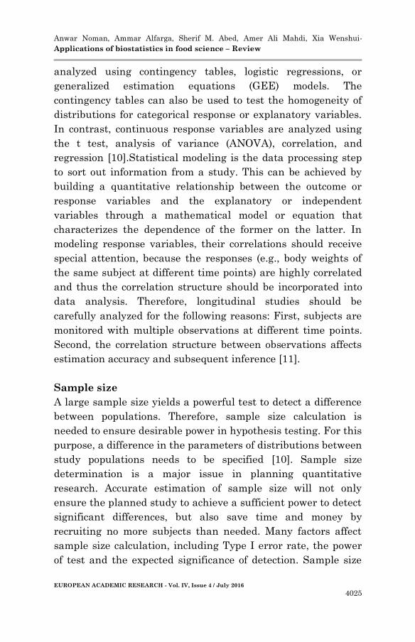
Sample size
A large sample size yields a powerful test to detect a difference
between populations. Therefore, sample size calculation is
needed to ensure desirable power in hypothesis testing. For this
purpose, a difference in the parameters of distributions between
study populations needs to be specified [10]. Sample size
determination is a major issue in planning quantitative
research. Accurate estimation of sample size will not only
ensure the planned study to achieve a sufficient power to detect
significant differences, but also save time and money by
recruiting no more subjects than needed. Many factors affect
sample size calculation, including Type I error rate, the power
of test and the expected significance of detection. Sample size

Anwar Noman, Ammar Alfarga, Sherif M. Abed, Amer Ali Mahdi, Xia Wenshui-
Applications of biostatistics in food science – Review
EUROPEAN ACADEMIC RESEARCH - Vol. IV, Issue 4 / July 2016
4026
calculation for studies not involving microarray or other high-
throughput technologies can be found in many biostatistics
books [12-13].
The aims of microarray studies include identification of
differentially expressed genes between cases and controls, as
well as profiling of subjects based on gene expression levels, the
main objective of microarray studies is to discriminate cases
fromcontrols. Two major classes of statistical models have been
studied so far. One class of models focuses on gene expression,
including the ANOVA method [14].and the t test-like method,
such as significance analysis of microarrays [15].
The ANOVA model-based approach
This approach rigorously depends on a statistical model for
data (i.e., the ANOVA model) where individual gene expression
or its transformation (usually a log transformation to ensure
the normality of intensity data) is assumed to be normally
distributed and analyzed using the ANOVA model. Popular
models are one-way or two-way ANOVA, incorporating
experimental design factors[16].described detailed modeling
and calculation based on the classical approach to sample size
determination for linear models with adjustments for multiple
comparisons through controlling type I error rate, FWER and
FDR. They then considered detailed sample size for several
standard microarray study designs, including matched-pair
data, completely randomized design, and isolated effect design.
A sample size table was also provided for each design. This
method can be assisted with a software package sizepower in R
[17].
Calculating the Standard Deviation
The standard deviation (s) is a measure of the deviation from
the mean. Note the dependence of S of the number of data
points. If the terms are all about the same, then the precision
should increase (S decreases) as N increases. So, it is

Anwar Noman, Ammar Alfarga, Sherif M. Abed, Amer Ali Mahdi, Xia Wenshui-
Applications of biostatistics in food science – Review
EUROPEAN ACADEMIC RESEARCH - Vol. IV, Issue 4 / July 2016
4027
statistically advantageous to make more measurements,
although this must be balanced with practical considerations.
Fig. 2. (A) Plot of six analytical values, mean 2.05, SD = 0.532; range 1.20 to
2.70; (B) plot of analytical values from 30 replicate samples, overlaid with a
ND curve forx = 30.3, s = 8.6. The data values are very slightly skewed but
otherwise conform well to a ND; (C) plot of microbiological colony counts on 25
samples (as colony forming units/g) overlaid with a ND plot for x = 10,600 and
s = 5360. Note that the data distribution shows a marked left-hand skew and
kurtosis. The data do not conform to a ND.
Normality of data
The normality of experimental results is an important premise
for the use of parametric statistical tests, such as analysis of
variance (ANOVA), correlation analysis, simple and multiple
regression and t-tests. If the assumption of normality is not
confirmed by relevant tests, interpretation and inference from
any statistical test may not be reliable or valid [18].

Anwar Noman, Ammar Alfarga, Sherif M. Abed, Amer Ali Mahdi, Xia Wenshui-
Applications of biostatistics in food science – Review
EUROPEAN ACADEMIC RESEARCH - Vol. IV, Issue 4 / July 2016
4028
Fig. 3. Comparison of two ND curves both having x = 10 g/l; curve A ( ) has s =
0.25 and B has s = 0.5 (… ). Note that more than 25% of the data values for
curve B fall outside the 95% CLs (9.5, 10.5) of the data in curve A.
Normality tests assess the likelihood that the given data set
{x1, …, xn}conforms to a ND. Typically, the null hypothesis H0
is that the observations are distributed normally, with
population mean μ and population variance σ2; the alternative
hypothesis Ha is that the distribution is not normal. It is
essential that the analyst identify the statistical distribution of
the data. Most chemical constituents and contaminants
conform well, or reasonably well, to a ND, but it is generally
recognized that microbiological data do not. Whilst microbial
colony counts generally conform to a lognormal distribution, the
numbers of cells in dilute suspensions generally approximate to
a Poisson distribution. The prevalence of very low levels of
specific organisms, especially pathogenic organisms such as
Cronobacter spp. and Salmonella spp., in infant feeds and other
dried foods show evidence of over-dispersion that is best
described by a negative-binomial or a beta-Poisson distribution
[19].
In practice, there are two ways to check experimental
results for conformance to a ND: graphically or by using
numerical methods. The graphical method, usually displayed by
normal quantile–quantile plots, histograms or box plots, is the
simplest and easiest way to assess the normality of data

Anwar Noman, Ammar Alfarga, Sherif M. Abed, Amer Ali Mahdi, Xia Wenshui-
Applications of biostatistics in food science – Review
EUROPEAN ACADEMIC RESEARCH - Vol. IV, Issue 4 / July 2016
4029
[20].Numerical approaches are the best way to test for the
normality of data, including determination of kurtosis and
skewness; for example, tests such as those attributed to
Anderson–Darling (AD), Kolmogorov–Smirnov (KS), Shapiro–
Wilk (SW), Lilliefors (LF), and Cramér von Mises (CM).
Frequently, people use histograms or probability plot graphs to
test for normality (when they do!), but it can be risky since it
does not provide quantitative proof that data follow ND. The
shape of the graph depends on the number of samples examined
and the number of bins used. Due to the small number of values
the data shown in Fig. 4 do not appear to follow a normal
distribution but the hypothesis of normality is not rejected by
tests.
Fig. 4. Histogram of data values overlaid with a ND plot. Although the data
do not appear to conform to a ND, tests for normality do not reject the null
hypothesis due to the small number of data: Kolmogorov–Smirnov: pKS N
0.20; Lillifors: pLillifors N 0.10, and Shapiro– Wilk: pSW = 0.68666.
[20]studied the power and efficiency of four tests (AD, KS, SW,
and LF) using Monte Carlo simulation and concluded that SW
is the most powerful test for all types of distribution and
sample sizes, whereas KS is the least accurate test. They also
confirmed that AD is almost comparable with SW and that LF
always outperforms KS. Using the example of Fig. 5, the SW
test gives p = 0.02355 b 0.05, so the null hypothesis is rejected
and the alternative hypothesis, that the data do not follow a
normal distribution, is accepted but if the KS test had been

Anwar Noman, Ammar Alfarga, Sherif M. Abed, Amer Ali Mahdi, Xia Wenshui-
Applications of biostatistics in food science – Review
EUROPEAN ACADEMIC RESEARCH - Vol. IV, Issue 4 / July 2016
4030
used p = 0.217 N 0.05 so the hypothesis of normality is not
rejected.
Fig. 5. Histogram of data values overlaid with a ND curve; the Shapiro–Wilk
(SW) rejects the hypothesis for normality (p = 0.0236) but the Kolmogorov–
Smirnov (KS) test (p N 0.20) does not reject the null hypothesis. The result
from the Lilliefors tests (p b 0.10) is indeterminate.
The moral is to choose your test with care and to understand its
limitations. In sensory and microbiological studies, for example,
it is very common to obtain results that do not follow a ND [21].
Parametric statistics in Food Science
Depending on the statistical distribution of data, sample size,
and homoscedasticity, samples and treatments can be compared
using parametric or non-parametric tests. Parametric tests
should be used when data are normally distributed and there is
homogeneity of variances, as shown by the Shapiro–Wilk and
Levene (or F) tests, respectively. Then, a Student's t-test is used
to check for differences between two mean values or an ANOVA
is used when three or more mean values need to be compared
(Fig. 6).
The ANOVA model-based approach
This approach rigorously depends on a statistical model for
data analysis (i.e., the ANOVA model) where individual gene

Anwar Noman, Ammar Alfarga, Sherif M. Abed, Amer Ali Mahdi, Xia Wenshui-
Applications of biostatistics in food science – Review
EUROPEAN ACADEMIC RESEARCH - Vol. IV, Issue 4 / July 2016
4031
expression or its transformation (usually a log transformation
to ensure the normality of intensity data) is assumed to be
normally distributed and analyzed using the ANOVA model.
Popular models are one-way or two-way ANOVA, incorporating
experimental design factors [10].
Fig. 6. Statistical steps and tests to compare two or more samples in relation
to a quantitative response variable.
Analysis of variances for three or more data sets
Analysis of variances (ANOVA) is a parametric statistical tool
that partitions the observed variance into components that
arise from different sources of variation. In its simplest form,
ANOVA provides a statistical test of whether or not the means
of several groups are all equal. In this sense, the null
hypothesis, H0, says there are no differences among results
from different treatments or sample sets; the alternative
hypothesis (Ha) is that the results to differ. If the null
hypothesis is rejected then the alternative hypothesis, Ha, is
accepted, i.e. at least one set of results differs from the others.
The ANOVA procedure should be used to compare the mean
values of three or more data sets. One practical example of

Anwar Noman, Ammar Alfarga, Sherif M. Abed, Amer Ali Mahdi, Xia Wenshui-
Applications of biostatistics in food science – Review
EUROPEAN ACADEMIC RESEARCH - Vol. IV, Issue 4 / July 2016
4032
application of analysis of variance is provided by [22] authors
investigated the rheological behavior of honeys from Spain
under different temperatures (25 °C, 30 °C, 35 °C, 40 °C, 45 °C,
and 50 °C) and concentrations and compared the samples using
one-way ANOVA followed by a test of multiple comparison of
means. Three alternative models can be used in an ANOVA:
fixed effects, random effects or mixed effects models. The fixed
effects model is appropriate when the levels of the independent
variables (factors) are set by the experimental design. The
random effects model, which is often of greatest interest to a
researcher, assumes that the levels of the effects are randomly
selected from an infinite population of possible levels [23].
Depending on the number of factors to be analyzed, we
can have:
-A one-way ANOVA in which only one factor is assessed.
This is the case for relatively simple comparisons of
physicochemical, colorimetric, chemical and microbiological
analyses [24-25-26-27]. For example, if five samples of apple are
analyzed for catechin content, the ―apples‖ are the independent
variable and the ―catechin content‖ is the dependent response
variable. Another important application of one-way ANOVA is
when different groups of test animals that are treated with an
extract/drug and compared to a control group [28].
-A 2-way ANOVA is used for two factors in which only
the main effects are analyzed. The 2-way ANOVA determines
the differences and possible interactions when response
variables are from two or more categories. The use of 2-way
ANOVA enables comparison and contrast of variables resulting
from independent or joint actions [29].This type of ANOVA can
be employed in sensory evaluation when both panelists and
samples are sources of variation [30]. Or when the consistency
of the panelists needs to be assessed.
-A factorial ANOVA for n factors, that analyzes the main
and the interaction effects is the most usual approach for many
experiments, such as in a descriptive sensory or microbiological

Anwar Noman, Ammar Alfarga, Sherif M. Abed, Amer Ali Mahdi, Xia Wenshui-
Applications of biostatistics in food science – Review
EUROPEAN ACADEMIC RESEARCH - Vol. IV, Issue 4 / July 2016
4033
evaluation of foods and beverages[31].A repeated-measures
(RM) ANOVA is used to analyze designs in which responses on
two or more dependent variables correspond to measurements
at different levels of one or more varying conditions.[32].used a
RM-ANOVA to examine results from assessments of different
instrumental color attributes for a mixture of juices from yacón
(Peruvian ground apple) tubers and yellow passion fruit as a
function of storage time.
The choice of post-hoc tests to be used should be decided
in advance so that bias is not attributed to any one set of data.
In recent times, so-called ‗robust‘ ANOVA methods have been
developed that are not affected by outlier data and can be used
when data do not conform strictly to ND. They were developed
following a need to analyze inter-laboratory studies during
validation of analytical methods for use in chemistry and
microbiology and are important also in determination of
measurement uncertainty estimates that are nowadays
required as part of laboratory accreditation [33].
Non-parametric statistics in Food Science
Non-parametric procedures use ranked data rather than actual
data values. The data are ranked from the lowest to the highest
and each value is assigned, in order, the integer values from 1
to n (where n = total sample size.. actual difference between
populations. Ranking for non parametric procedures preserves
information about the order of the data but discards the actual
values. Because information is discarded, non-parametric
procedures can never be as powerful (i.e. less able to detect
differences) as their parametric counterparts [34].

Anwar Noman, Ammar Alfarga, Sherif M. Abed, Amer Ali Mahdi, Xia Wenshui-
Applications of biostatistics in food science – Review
EUROPEAN ACADEMIC RESEARCH - Vol. IV, Issue 4 / July 2016
4034
Table 1: Use of the Wilcoxon Signed Ranks test to determine the level
of patulin in lots of apple compote (legal limit 25 μg/kg) using two
analytical methods (A & B)
Tabulate the results for methods A & B, then determine the
difference (A − B). Ignoring the sign and any zero value allocate
a rank to each difference, using an average rank if results are
identical. Then allocate the relevant sign to each rank. Add the
rank scores for R+ and R− and, for the number of pairs (in this
case n = 9), compare the smaller rank total with the tabulated
value in tables of Wilcoxon's signed ranks. If, as in this case,
the smaller rank total is ≤ published value then the difference
is statistically significant at p = 0.05. Hence the null
hypothesis, that results from both methods are equal, should be
rejected as method A gives higher results. Whether the
differences are of practical importance is another matter!
Table 2: Comparison of bacterial numbers on cotton and plastic
sponge swabs taken from chicken neck skins immediately after
evisceration.

Anwar Noman, Ammar Alfarga, Sherif M. Abed, Amer Ali Mahdi, Xia Wenshui-
Applications of biostatistics in food science – Review
EUROPEAN ACADEMIC RESEARCH - Vol. IV, Issue 4 / July 2016
4035
Allocate ranks (1–20) across both sets of data; average the rank
for identical counts (in this case, counts of 110). Calculate the
rank totals: RA = 88.5; RB = 121.5. Calculate the UA statistic
for data set A: UA = [nA(nA + 1) / 2 + nAnB − RA] = 66.5.
Similarly, calculate the UB statistic for data set B: UB = 33.5.
Take the smaller value of U as the test statistic and compare it
with the Mann–Whitney tabulated value for p = 0.05 with nA =
nB = 10. The calculated value of UB (33.5) N Ucritical (23) so
the null hypothesis that both methods give equal results is not
rejected — the 2-tailed probability is p = 0.25.
Table 3. Non-parametric analysis of the scores from a wine tasting
Number of samples = n = 6. We determine a value M using the
equation: M ¼ nk k ð Þ 12 þ1 ∑R2 k−3n k ð Þ þ 1. For these
data, M = 4.233 with υ = k − 1 = 4 degrees of freedom.
From the Tables, we find that the critical value for χ2(p = 0.05,
υ = 4) is 9.49 which is greater than M and therefore we do not
reject the null hypothesis that the tasters have scored the
samples uniformly. Full details of these, and other
nonparametric and parametric tests, are given in standard
works including [35].
Bivariate correlation analysis
Correlation is a method of analysis used to study the possible
association between two continuous variables. The correlation
coefficient (r) is a measure that shows the degree of association
between both variables [36].This parametric test requires both

Anwar Noman, Ammar Alfarga, Sherif M. Abed, Amer Ali Mahdi, Xia Wenshui-
Applications of biostatistics in food science – Review
EUROPEAN ACADEMIC RESEARCH - Vol. IV, Issue 4 / July 2016
4036
data sets to consist of independent random variables that
conform to ND. The correlation coefficient measures the degree
of linear association between the two sets of data (A and B), and
its value lies between −1 and +1. The closer the absolute value,
|r|, is to 1, the stronger the correlation between the data
values [37].The correlation between two variables is positive
(Fig. 7A) if high values for one variable are associated with high
values for the other variable and negative (Fig. 7B) if one
variable is low when the other is high. A correlation close to r =
0 (Fig. 7C) indicates that there is no linear relation, or at best a
very weak correlation, between the two variables. However, a
low r-value does not necessarily imply that there is no
relationship between the responses; a low value can be due to
the existence of a non-linear correlation between these
variables, but the presence of outliers in one or both data sets
may also affect the r-value [38].
Many workers calculate the Pearson linear correlation
coefficient in order to seek to determine the strength of
association between data sets. However, when more than five
variables are analyzed, the analysis is compromised because
correlation coefficients do not assess simultaneous association
among results for all variables, which makes it difficult to
understand and interpret the structure and patterns of the
data. For example, if one considers five sets of response
variables (A, B, C, D and E), it is necessary to calculate the
correlation coefficients, and their significance, for each data set
pair, i.e. AB, AC, AD, AE, BC, BD, BE, CD, CE, and DE. It is
easy to understand and interpret up to three correlations
coefficients but, in order to better understand multiple
responses, a more sophisticated multivariate statistical
approach, such as principal component analysis, clustering
techniques, linear discriminant analysis should be used [39].
When large sets of results (≥30) are analyzed, data
should be formally checked for normality. If the data do not
follow a normal distribution a non-parametric approach, such

Anwar Noman, Ammar Alfarga, Sherif M. Abed, Amer Ali Mahdi, Xia Wenshui-
Applications of biostatistics in food science – Review
EUROPEAN ACADEMIC RESEARCH - Vol. IV, Issue 4 / July 2016
4037
as the Spearman's rank correlation coefficient, should be used
to analyze for any correlation between the responses. Fig. 9
shows the steps to follow when two data sets (each with n ≥ 8)
are to be analyzed with respect to correlation. Spearman's
correlation coefficient (ρ) should be used when either or both
data sets do not conform to ND, when the sample size is small,
or when the variables are measured as ordinals i.e. first, fifth,
eighth, etc. in a sequence of values. The Spearman correlation
coefficient does not require the assumption that the
relationship between variables is linear. One good example to
compare both Pearson and Spearman correlation coefficients
can be obtained by analyzing the data sets below:
A: 12.56; 14.46; 16.65; 25.68; 16.80; 28.95; 32.25; 30.33;
32.81; 28.29; 29.98; 30.32; 33.57
B: 53.25; 65.33; 53.68; 62.74; 61.53; 64.89; 66.40; 60.99; 68.50;
56.30; 66.36; 68.25; 73.89

Anwar Noman, Ammar Alfarga, Sherif M. Abed, Amer Ali Mahdi, Xia Wenshui-
Applications of biostatistics in food science – Review
EUROPEAN ACADEMIC RESEARCH - Vol. IV, Issue 4 / July 2016
4038
Fig. 7. (A) Positive correlation, (B) negative correlation, and (C) almost null
correlation.
There are two major concerns regarding correlation tests: the
significance of the correlation and the interpretation of results.
Firstly, to assume a statistically significant association between
variables the p-value of the correlation coefficient should be
b˂.05[40].showed that with large data sets, the correlation
coefficient is often statistically significant even at a moderate or
low r value. On the other hand, when the data set is small [41].
Fig.8. Steps to follow when two data sets (usually wi)
the n ≥ 8 are to be analyzed for correlation.

Anwar Noman, Ammar Alfarga, Sherif M. Abed, Amer Ali Mahdi, Xia Wenshui-
Applications of biostatistics in food science – Review
EUROPEAN ACADEMIC RESEARCH - Vol. IV, Issue 4 / July 2016
4039
Regression analysis
Assumptions for regression require that:
– The samples are representative of the population for the
inference prediction.
– The concentrations of the independent variables are
measured with error, i.e. they are ‗absolute‘ values; if this is not
the case then the more complex orthogonal linear regression
must be used in order to correct for errors in the predictor
variable[42].
– The error term of the estimates is a random variable with
zero mean;
– The predictors are linearly independent, i.e. each value
cannot be expressed as a linear combination of the other values.
1. The variance of the errors is homoscedastic. In order to
perform a regression analysis it is essential to:
2. Test data for the presence of outliers (at 95 or 99% of
confidence) using the Grubb's test for each concentration
level.
3. Ensure the homogeneity of variances in the
concentration levels of the calibration curve by using one
the tests.
4. Test the significance of the regression and its lack of fit
through the F-test and a one-factor ANOVA. Provided
that the response is directly and linearly correlated to
the concentrations then the regression coefficient should
be significant. Evidence for lack of fit (p ˂ 0.05), may be
due to a non-linear response, to excessive variation in
the replicates at one or more of the test values or the use
of an over-extended independent variable range. In this
case, removing the highest values and repeating the
statistical analysis should reduce the range of
concentrations. Evidence for lack of linearity may
indicate that a nonlinear model (quadratic, for example)
might be more appropriate for the method, and
therefore, alternative models should be evaluated.

Anwar Noman, Ammar Alfarga, Sherif M. Abed, Amer Ali Mahdi, Xia Wenshui-
Applications of biostatistics in food science – Review
EUROPEAN ACADEMIC RESEARCH - Vol. IV, Issue 4 / July 2016
4040
5. Determine the following statistical parameters by means
of the regression analysis:
• The regression equation (y = ax + b), where y is the dependent
estimate at independent concentration level (x), (a) is the slope
of the line and b is the linear intercept when x = 0.
• The standard deviation of the estimated parameters and
model;
• The statistical significance of the estimated parameters;
• The coefficient of determination (R2; regression coefficient)
and the adjusted R2.
The regression model is considered suitable to the
experimental data when:
1. The standard deviation of the parameter is at least 10%
lower than the corresponding parameter value.
2. The standard deviation of the proposed mathematical model
is small;
3. The parameters of a model are statistically significant
otherwise they will not contribute to the model.
It is a myth to consider that if R2˃ 90% the model is
excellent this is only one criterion to evaluate the goodness of fit
of the model. If R2 is low (˂70%), the mathematical model is not
good; on the other hand, if R2 is high (˃90%), it means that you
should continue the analysis and check the other criteria. It is
noteworthy that in some applications, depending on the type of
analysis, e.g. evaluation of sensory data, the coefficient of
determination may be considered well if R2˃ 60%.
4. The statistical significance, obtained from the F-test of an
ANOVA analysis of the proposed mathematical model is at
least p ˂ 0.05.
5. Analysis of the residuals (experimental value for a response
variable minus value predicted by the mathematical model)
must conform to ND and have a constant variance, as described
above. This is a necessary condition for the application of some
post-hoc tests such as t and F. It is important to recognize that
the regression and correlation coefficients describe different

Anwar Noman, Ammar Alfarga, Sherif M. Abed, Amer Ali Mahdi, Xia Wenshui-
Applications of biostatistics in food science – Review
EUROPEAN ACADEMIC RESEARCH - Vol. IV, Issue 4 / July 2016
4041
parameters. Regression describes the goodness of fit of a model;
correlation estimates the linear relationship of two variables. A
common mistake is to use R2 to compare models. R2 is always
higher if we increase the order of a model (linear in comparison
to quadratic, for example). For example, a third order
polynomial has a higher R2 than a second order polynomial
because there are more terms, but it does not necessarily mean
that the first is the better model. An analysis of the degrees of
freedom (number of experimental points minus number of
parameters from the model) needs to be carried out. A model
with more terms requires estimation of more coefficients so
fewer degrees of freedom remain. Thus, another criterion needs
to be used: the adjusted regression coefficient — R2adj . This
coefficient adjusts for the number of explanatory terms in a
model relative to the number of data points and its value is
usually less than or equal to that of R2. When comparing
models, the one with the highest adjusted coefficient is the best
model.
We have noted above that in addition to simple
‗Generalized Linear Models‘ of regression other, more complex,
forms of regression are available for use in specific
circumstances. The reader is directed to other works, such as
[43].for information and guidance on such procedures.
REFERENCES
1-He QH, Kong XF, Wu G, Ren PP, Tang HR, Hao FH, et al. (
2009). Metabolomic analysis of the response of growing pigs to
dietary L-arginine supplementation. Amin Acids;37:199–208.
2-Karlin S. (2005). Statistical signals in bioinformatics.
ProcNatlAcadSci U S A ;102: 13355–62.
3-Fu WJ, Haynes TE, Kohli R, Hu J, Shi W, Spencer TE, et al
(2005). Dietary L-arginine supplementation reduces fat mass in
Zucker diabetic fatty rats. J Nutr ;135: 714–21.

Anwar Noman, Ammar Alfarga, Sherif M. Abed, Amer Ali Mahdi, Xia Wenshui-
Applications of biostatistics in food science – Review
EUROPEAN ACADEMIC RESEARCH - Vol. IV, Issue 4 / July 2016
4042
4-Nguyen DV, Arpat AB, Wang N, Carroll RJ (2002). DNA
microarray experiments: Biological and technological aspects.
Biometrics 2002;58:701–17.
5-Fu WJ, Hu J, Spencer T, Carroll R, Wu G (2006). Statistical
models in assessing fold changes of gene expression in real-time
RT-PCR experiments. Comput Biol Chem ;30: 21–26.
6-Bergstrand, M., &Karlsson, M.O. (2009). Handling data below
the limit of quantification in mixed effect models. The AAPS
Journal, 11(2), 371–380.
7-Baert, K., Meulenaer, B., Verdonck, F., Huybrechts, I.,
Henauw, S., Vanrolleghem, P. A., et al.(2007). Variability and
uncertainty assessment of patulin exposure for preschool
children in Flanders. Food and Chemical Toxicology, 45(9),
1745–1751.
8-Lorrimer, M. F., &Kiermeier, A. (2007). Analyzing
microbiological data — Tobit or not Tobit. International Journal
of Food Microbiology, 116, 313–318.
9-Jarvis, B. (2008). Statistical aspects of the microbiological
examination of foods (2nd ed.) London: Academic Press.
10-Fu WJ., Stromberg A.,Viele K.,Carroll R., Wu G., (2010)
Statistics and bioinformatics in nutritional sciences: analysis of
complex data in the era of systems biology. Journal of
Nutritional Biochemistry 2010;21:561–572.
11-Benjamini Y, Hochberg Y(1995). Controlling the false
discovery rate: a practical and powerful approach to multiple
testing. J Royal Stat Soc Series B ;57: 289–300.
12-Rosner B. (2005). Fundamentals of Biostatistics. 6th ed.
New York (NY): Duxbury Press.
13-Fleiss JL, Levin B, Paik MC. (2003). Statistical Methods for
Rates and Proportions. 3rd ed. New York (NY): Wiley.
14-Kerr MK, Martin M, Churchill GA.(2000). Analysis of
variance for gene expression microarray data. J
ComputBiol;7:819–37.

Anwar Noman, Ammar Alfarga, Sherif M. Abed, Amer Ali Mahdi, Xia Wenshui-
Applications of biostatistics in food science – Review
EUROPEAN ACADEMIC RESEARCH - Vol. IV, Issue 4 / July 2016
4043
15-Tusher VG, Tibshirani R, Chu G. (2001). Significance
analysis of microarrays applied to the ionizing radiation
response. ProcNatlAcadSci U S A;98:5116–21.
16-Kerr MK, Churchill GA (2001). Statistical design and the
analysis of gene expression microarray data. Genet Res
Camb;77:123–8.
17-Qiu W, Lee MLT, Whitmore GA (2015). Sample size and
power calculation in microarray studies using the sizepower
package. Technical report, Bioconductor. http://
bioconductor.org/packages/2.2/bioc/vignettes/sizepower/inst/doc/
sizepower.
18-Shapiro, S. S., &Wilk, M. (1965). An analysis of variance test
for normality (complete samples). Biometrika, 52, 591–611.
19-Jongenburger, I. (2012). Distributions of microorganisms in
foods and their impact on food safety. (PhD Thesis). NL:
University of Wageningen.
20-Razali, N. M., &Wah, Y. B. (2011). Power comparisons of
Shapiro–Wilk, Kolmogorov- Smirnov, Lilliefors and Anderson–
Darling tests. Journal of Statistical Modeling and Analytics, 2,
21–33.
21-Granato, D., Ribeiro, J. C. B., Castro, I. A., & Masson, M. L.
(2010). Sensory evaluation and physicochemical optimisation of
soy-based desserts using response surface methodology. Food
Chemistry, 121(3), 899–906.
22-Oroian, M., Amariei, S., Escriche, I., &Gutt, G. (2013).
Rheological aspects of Spanish honeys. Food Bioprocess
Technology, 6, 228–241.
23-Calado, V. M.A., & Montgomery, D. C. (2003). Planejamento
de ExperimentosusandoStatistica. Rio de Janeiro: e-papers (1st
ed.) (Available at: www.e-papers.com.br (last accessed 2 July
2013).
24-Alezandro, M. R., Granato, D., Lajolo, F. M., & Genovese, M.
I. (2011). Nutritional aspects of second generation soy foods.
Journal of Agricultural and Food Chemistry, 59, 5490–5497.

Anwar Noman, Ammar Alfarga, Sherif M. Abed, Amer Ali Mahdi, Xia Wenshui-
Applications of biostatistics in food science – Review
EUROPEAN ACADEMIC RESEARCH - Vol. IV, Issue 4 / July 2016
4044
25-Corry, J. E. L., Jarvis, B., Passmore, S., & Hedges, A. J.
(2007). A critical review of measurement uncertainty in the
enumeration of food microorganisms. Food Microbiology, 24,
230–253.
26-Granato, D., Freitas, R. J. S., & Masson, M. L. (2010).
Stability studies and shelf life estimation of a soy-based
dessert. Ciência e Tecnologia de Alimentos, 30, 797–807.
27-Oroian, M. (2012). Physicochemical and rheological
properties of Romanian honeys. Food Biophysics, 7, 296–307.
28-Macedo, L. F. L., Rogero, M. M., Guimarães, J. P., Granato,
D., Lobato, L. P., & Castro, I. A. (2013). Effect of red wines with
different in vitro antioxidant activity on oxidative stress of
high-fat diet rats. Food Chemistry, 137, 122–129.
29-MacFarland, T. W. (2012). Two-way analysis of variance —
Statistical tests and graphics using R. Springer, 150.
30-Granato, D., Ribeiro, J. C. B., & Masson, M. L. (2012).
Sensory acceptability and physical stability assessment of a
prebiotic soy-based dess.
31-Ellendersen, L. S. N., Granato, D., Guergoletto, K. B.,
&Wosiacki, G. (2012). Development and sensory profile of a
probiotic beverage from apple fermented with Lactobacillus
casei. Engineering in Life Sciences, 12(4), 475–485.
32-Benincá, C., Granato, D., Castro, I. A., Masson, M. L.,
&Wiecheteck, F. V. B. (2011). Influence of passion fruit juice on
colour stability and sensory acceptability of non-sugar
yacon-based pastes. Brazilian Archives of Biology and
Technology, 54, 149–159.
33-Elison, S. L. R., Rosslein, M., & Williams, A. (Eds.). (2000).
Quantifying uncertainty in analytical measurement (2nd ed.):
Eurachem/Citac.
34-Hollander, M., & Wolfe, D. A. (1973). Nonparametric
statistical methods. New York: John Wiley & Sons, Inc.
35-Sheskin, D. J. (2011). Handbook of parametric and
nonparametric statistical procedures (5th ed.): Chapman-
Hall/CRC.

Anwar Noman, Ammar Alfarga, Sherif M. Abed, Amer Ali Mahdi, Xia Wenshui-
Applications of biostatistics in food science – Review
EUROPEAN ACADEMIC RESEARCH - Vol. IV, Issue 4 / July 2016
4045
36-Granato, D., Calado, V., Oliveira, C. C., & Ares, G. (2013).
Statistical approaches to assess the association between
phenolic compounds and the in vitro antioxidant activity of
Camellia sinensis and Ilex paraguariensis teas. Critical
Reviews in Food Science and Nutrition.
http://dx.doi.org/10.1080/10408398.2012.750233.
37-Ellison, S. L. R., Barwick, V. J., &Farrant, T. J.D. (2009).
Practical statistics for the analytical scientist — A bench guide.
Cambridge: RSC Publishing.
38-Altman, D.G. (1999). Practical statistics for medical research
(8th ed.)Boca Raton: Chapman& Hall/CRC, 611.
39-Besten, M.A., Jasinski, V. C. G., Costa, A. G. L. C., Nunes,
D. S., Sens, S. L., Wisniewski, A., Jr., et al. (2012). Chemical
composition similarity between the essential oils isolated from
male and female specimens of each five Baccharis species.
Journal of the Brazilian Chemical Society, 23, 1041–1047.
40-Granato, D., Katayama, F. C. U., & Castro, I. A. (2011).
Phenolic composition of South American red wines classified
according to their antioxidant activity, retail price and sensory
quality. Food Chemistry, 129, 366–373.
41-Granato, D., Freitas, R. J. S., & Masson, M. L. (2010).
Stability studies and shelf life estimation of a soy-based
dessert. Ciência e Tecnologia de Alimentos, 30, 797–807.
42-Carroll, R. J., Ruppert, D., Stefanski, L. A., &Crainiceanu,
C. M. (2012). Measurement error in non-linear models (2nd ed.):
Chapman Hall/CRC Press.
43-Kleinbaum, D., Kupper, L., &Azhar, N. (2007). Applied
regression analysis and multivariate methods (4th ed.)
Thomson Brooks/Cole; Duxbury, Belmont, Ca, USA.