Application of Wavelet and Regression Analysis in Assessing Temporal and Geographic Climate

Application of Wavelet and Regression Analysis in AssessingTemporal and Geographic Climate Variability: Eastern Ontario,

Canada as a Case Study

Andreas Prokoph1* and R. Timothy Patterson2

1SPEEDSTAT, 36 Corley Private, Ottawa, ON, K1V 8T7 2Department of Earth Sciences and Ottawa-Carleton Geoscience Centre,

Herzberg Building, Carleton University, Ottawa, ON

[Original manuscript received 10 November 2003; in revised form 23 April 2004]

ABSTRACT Regression and wavelet analysis have been employed to trace and quantify variation in temporal pat-terns (e.g., cycles and trends) between the instrument climate records of urban Ottawa and nearby rural areas ineastern Ontario. Possible links between observed climate change at these stations and possible natural andanthropogenic drivers were also investigated. Regression analysis indicates that the temperature in Ottawaincreased, on average, at a rate of >0.01°C yr–1 in comparison to adjacent rural areas over the last century.Wavelet analysis shows that this relative urban warming trend was primarily manifested in the form of multi-decadal and interseasonal cycles that are likely attributable to gradual increased winter heating in Ottawa (heatisland effects) associated with population growth. We estimate that the 1°C increase in the Ottawa temperatureis equivalent to an increase in population size of ~400,000. In contrast, interannual variability correlates wellbetween rural and urban areas with about the same temperature amplitudes.

RÉSUMÉ [traduit par la rédaction] On a utilisé l’analyse de la régression et des ondelettes pour discerner et quantifier la variation dans les configurations temporelles (p. ex., cycles et tendances) entre les relevés climatologiques instrumentaux dans la région urbaine d’Ottawa et dans la région rurale avoisinante de l’Estde l’Ontario. On étudie aussi les liens possibles entre le changement climatique observé à ces stations etd’éventuelles causes naturelles ou anthropiques. L’analyse de régression indique que, durant le dernier siècle, la température, à Ottawa, a augmenté à un rythme annuel moyen supérieur à 0,01 °C, par comparaisonaux régions rurales adjacentes. L’analyse des ondelettes montre que cette tendance au réchauffement urbainrelatif s’est principalement manifestée sous la forme de cycles multidécennaux et intersaisonniers vraisemblablement attribuables à une augmentation du chauffage en hiver à Ottawa (effets d’îlot de chaleur),augmentation liée à l’accroissement démographique. Nous estimons que l’augmentation de température de1 °C à Ottawa équivaut à un accroissement de la taille de la population de ~400 000. Par contraste, la variabilité interannuelle est bien corrélée entre les régions rurales et urbaines, avec à peu près les mêmesamplitudes de température.

ATMOSPHERE-OCEAN 42 (3) 2004, 201–212© Canadian Meteorological and Oceanographic Society

*Corresponding author’s e-mail: [email protected]

1 Introduction

Statistical analysis of worldwide observational temperaturerecords has revealed a global temperature increase of0.3°–0.7°C over the last century (IPCC, 1996). In the north-ern hemisphere most of this increase has been attributed to adecrease in diurnal temperature range, suggesting that condi-tions are actually ‘less cold’ rather than ‘warmer’ (e.g.,Bonsal et al., 2001). This warming has alternatively beenlinked to an increase in anthropogenic greenhouse gas CO2output (IPCC, 1996), a growing urban heat island effect as

North American urban centres have grown in size (Karl et al.,1988), or natural processes such as changes in solar radiation(e.g., Carslaw et al., 2002).

Urban heat islands are the result of numerous anthro-pogenic heat sources, decreased evapotranspiration relatedto construction material heat storage, and a decrease inlongwave radiation loss due to a reduction in sky view factors(e.g., Oke, 1982; Gallo et al., 1996, 1999). Temperature increas-es due to the heat island effect vary with the square root of

mailto:[email protected]

population size, varying from 0.06°C for a population of~2,000 to ~0.7°C for a population of 500,000 (Karl et al.,1988). Thus, temperature variability, including long-termtrends, recorded in, or near, urban centres is not necessarilyrepresentative of global or even regional temperature changes(e.g., Quereda Sala et al., 2000). It has been estimated thatsouthern Canada warmed between 0.5° and 1.5°C during thetwentieth century due to several sources of anthropogenicwarming, including greenhouse gases (Bonsal et al., 2001;Zhang et al., 2000).

A potentially valuable tool for discriminating temporaland geographic climate variability is wavelet analysis.Wavelet analysis emerged as a filtering and data compres-sion method in the 1980s (e.g., Morlet et al., 1982). Sincethen, it has been widely applied in many disciplines (e.g.,Grossman and Morlet, 1984). This methodology hasrecently been used to trace changes in trends and cycles,rainfall variability (e.g., Nakken, 1999), solar irradiance,and interdecadal climate oscillations (e.g., Oh et al., 2002;Lucero and Rodriguez, 2000) over time. In the last decadeautoregressive moving-average (ARMA) (e.g., Karl et al.,1991), ‘analysis of variance’ (ARIMA) (e.g., Zwiers andKharin, 1998) and regression models (e.g., Vincent, 1998)have also been used to evaluate possible climate change scenarios and inhomogeneities within climate records. The detection of non-stationarities (i.e., interruptions or non-persistence in the temperature variability record) isparticularly crucial when making statistical inferences(e.g., Katz, 1988; Bunde et al., 2001). These earlier inho-mogeneity analysis models filtered out inhomogeneities asdifferences compared to specific trends (i.e., regressivetrend) or bandwidths (i.e., by using low-pass filters utiliz-ing moving averages, while wavelet-transform presentsinhomogeneities in time series as the sum of temporalchanges in the amplitude and phase of records over a widesine-wave bandwidth.

Our objectives for this case study are to: (1) Discriminate the variability associated with trends,

cyclic components, and non-stationarities (e.g., inhomogeneities) in temperature records from easternOntario;

(2) Apply time-series analysis methodology to monthlytemperature records, monthly records of urban-rural dif-ferences, and to records of differences in interseasonaltemperature variance between urban (Ottawa) and ruralareas (Morrisburg, Maniwaki) in eastern Canada;

(3) Assess whether any differences observed in temperaturepatterns can be linked to human influence (e.g., devel-opment of an urban heat island effect).

2 Time series analysis methodsa Wavelet AnalysisOne approach used to understand climatic signals better (i.e.,temperature records) is to extract the relevant informationfrom a temperature time series by transforming them. The tra-

ditional way to extract periodic features is to utilize a Fouriertransform. Unfortunately, the Fourier transform is limitedbecause a single analysis window cannot detect features in thesignals that are either much longer or shorter than the windowsize. ‘Moving-window’ Fourier transform (MWFT) slides afixed-size analysis window along the time axis and is able todetect non-stationarities (e.g., Rioul and Vetterli, 1991). Thefixed size window algorithm of MWFT limits the detection ofcycles at wavelengths that are longer than the analysis win-dows, and non-stationarities in short wavelengths (i.e., highfrequencies) are smoothed. Use of the wavelet transformsolves this problem, because it uses narrow windows at highfrequencies, and wide windows at low frequencies (Fig. 1).

Thus, wavelet analysis permits an automatic localization ofobjects, such as periodic-cyclic sequences, in time, space, andfrequency domains including data reduction and signal filter-ing (e.g., Rioul and Vetterli, 1991). The features of thewavelet transform and properties of its various analysis func-tions (‘mother wavelets’) have been widely studied, andbooks by Kaiser (1993) and Daubechies (1992) provide anoverview of the variety of different wavelet analysis tech-niques available.

For this time-series study, the capacity of a one-dimensional wavelet transform that will be utilized for automatic local-ization of periodic-signals, gradual shifts, and abrupt inter-ruptions (discontinuities), will be exploited. The waveletcoefficients, W, of a time series, x(s), are calculated by a sim-ple convolution:

(1)

where ψ is the mother wavelet; the variable a is the scale fac-tor that determines the characteristic wavelength (=1/frequen-cy); and b represents the shift of the wavelet over, x(s), (Chaoand Naito, 1995). The wavelet coefficients, W, are normalizedto represent the amplitude of Fourier frequencies.

We have utilized a continuous wavelet transform, with theMorlet wavelet as the mother function (Morlet et al., 1982).The Morlet wavelet is simply a sinusoid with a wave-length/period, a, modulated by a Gaussian function (Fig. 1),and has provided robust results in analyses of climate-relatedrecords (Prokoph and Barthelmes, 1996; Appenzeller et al.,1998; Gedalof and Smith, 2001). The shifted and scaled Morlet mother wavelet is defined as:

(2)

The parameter l addresses Heisenberg’s uncertainty principle(e.g., Rioul and Vetterli, 1991) that the location and velocityof objects cannot be measured at maximum precision simul-taneously. Thus l is used to modify the wavelet transformbandwidth-resolution either in favour of time or in favour of

202 / Andreas Prokoph and R. Timothy Patterson

W a ba

x ss b

adsψ ψ,( ) =

( ) −

∫1

ψ ππ

a bl

ia

s bs al e e

s b

al

, ( ) .( ) =− − − −

− −( )

14

12

12

2

21

frequency, and represents the length of the mother wavelet.The bandwidth resolution, ∆a/a, for the wavelet transformvaries with

(3)

and a location resolution . (4)

The parameter l = 10 is chosen for all analyses, which givessufficiently precise results in resolving depth and frequencyrespectively (Prokoph and Barthelmes, 1996; Ware andThomson, 2000). The relative bandwidth resolution, ∆a/a, is,according to Eq. (3), a constant for all scales.

The wavelet coefficients at the beginning and end of thedata are subject to ‘edge effects’, because only half of theMorlet wavelet lies inside the dataset. The missing data forthe analysis window therefore have to be replaced (‘padded’)by zeros. For long wavelengths (e.g., wavelength a covers

more than half of the whole data series), the edge effect canstretch across the entire time series. Thus, the boundary ofedge effects on the wavelet coefficients forms a wavelengthdependent curve for the 50% ‘edge-effect free’ areas knownas the ‘cone of influence’ (Torrence and Compo, 1998).

To transform a measured, and hence limited and discretetime-series, the integral in Eq. (1) has to be modified to a numer-ical solution by using the trapezoidal rule for unevenly sampledpoints. This evaluation of the wavelet transform, provides anestimate W*l(a,b) (Prokoph and Barthelmes, 1996). Visualizationof the values W*l(a,b) has been carried out using interpolationand coding with appropriate colours or shades of grey. In ourapproach, we used four shades of grey, including white andblack, to represent ranges of amplitudes of the underlying sinu-soidal signals. Prokoph and Barthelmes (1996) describe themethod and computer program CWTA.F utilized in detail.

b Synthetic ModelThe differences in time-frequency resolution obtained usingboth methods are illustrated in Fig. 2. In both cases thewavelet scalogram and periodogram obtained using a discrete

Wavelet and Regression Analysis of Climate Variability in Eastern Ontario / 203

∆a

a l= 2

4π,

∆bal=2

Fig. 1 Schematic presentation of analysis windows and bandwidth uncertainties for (a) continuous wavelet analysis (simplified for a dyadic wavelet) includingthe real part of Morlet wavelet (bottom) and region of influence of a single signal spike (b = b1), (b) Fourier transform.

a b

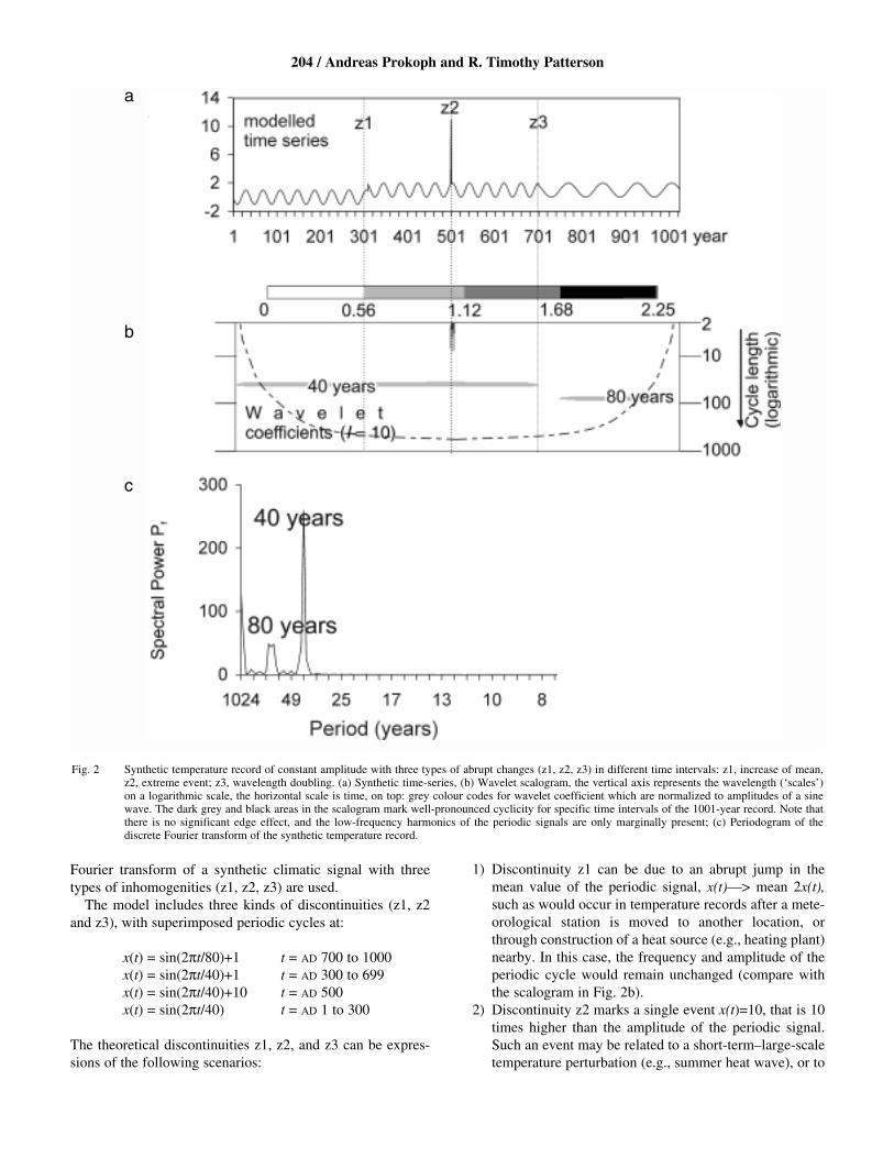
Fourier transform of a synthetic climatic signal with threetypes of inhomogenities (z1, z2, z3) are used.

The model includes three kinds of discontinuities (z1, z2and z3), with superimposed periodic cycles at:

x(t) = sin(2πt/80)+1 t = AD 700 to 1000x(t) = sin(2πt/40)+1 t = AD 300 to 699x(t) = sin(2πt/40)+10 t = AD 500x(t) = sin(2πt/40) t = AD 1 to 300

The theoretical discontinuities z1, z2, and z3 can be expres-sions of the following scenarios:

1) Discontinuity z1 can be due to an abrupt jump in themean value of the periodic signal, x(t)—> mean 2x(t),such as would occur in temperature records after a mete-orological station is moved to another location, orthrough construction of a heat source (e.g., heating plant)nearby. In this case, the frequency and amplitude of theperiodic cycle would remain unchanged (compare withthe scalogram in Fig. 2b).

2) Discontinuity z2 marks a single event x(t)=10, that is 10times higher than the amplitude of the periodic signal.Such an event may be related to a short-term–large-scaletemperature perturbation (e.g., summer heat wave), or to


Fig. 2 Synthetic temperature record of constant amplitude with three types of abrupt changes (z1, z2, z3) in different time intervals: z1, increase of mean,z2, extreme event; z3, wavelength doubling. (a) Synthetic time-series, (b) Wavelet scalogram, the vertical axis represents the wavelength (‘scales’)on a logarithmic scale, the horizontal scale is time, on top: grey colour codes for wavelet coefficient which are normalized to amplitudes of a sinewave. The dark grey and black areas in the scalogram mark well-pronounced cyclicity for specific time intervals of the 1001-year record. Note thatthere is no significant edge effect, and the low-frequency harmonics of the periodic signals are only marginally present; (c) Periodogram of the discrete Fourier transform of the synthetic temperature record.

a

b

c

a measurement error, and is detectable using bothwavelet and discontinuity analysis.

3) Discontinuity z3 describes an abrupt doubling of period-icity and accumulation rate, perhaps related to changingintervals between El Niño events, and is easily detectableby wavelet analysis.

In contrast, analysis carried out using single-windowedFourier analysis cannot be used to detect temporal disconti-nuities, nor can it be used to distinguish between continuouslow-amplitude and non-stationary high-amplitude signals.Single-window Fourier analysis also does not yield informa-tion on the temporal persistence of periodicities (Fig. 2c).

The wavelet and spectral analysis methodology utilized foranalysis of the synthetic climate record described above takesthe same approach as used to analyse the actual climatic datautilized in this study.

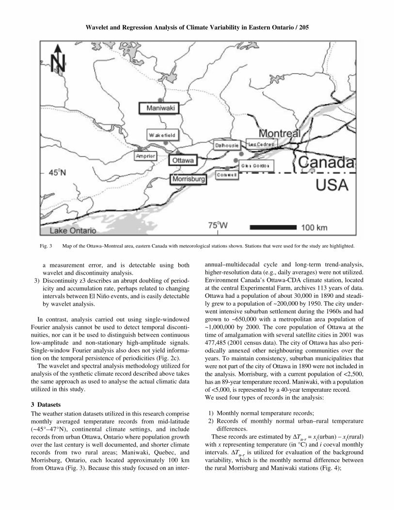
3 DatasetsThe weather station datasets utilized in this research comprisemonthly averaged temperature records from mid-latitude(~45°–47°N), continental climate settings, and includerecords from urban Ottawa, Ontario where population growthover the last century is well documented, and shorter climaterecords from two rural areas; Maniwaki, Quebec, andMorrisburg, Ontario, each located approximately 100 kmfrom Ottawa (Fig. 3). Because this study focused on an inter-

annual–multidecadal cycle and long-term trend-analysis,higher-resolution data (e.g., daily averages) were not utilized.Environment Canada’s Ottawa-CDA climate station, locatedat the central Experimental Farm, archives 113 years of data.Ottawa had a population of about 30,000 in 1890 and steadi-ly grew to a population of ~200,000 by 1950. The city under-went intensive suburban settlement during the 1960s and hadgrown to ~650,000 with a metropolitan area population of~1,000,000 by 2000. The core population of Ottawa at thetime of amalgamation with several satellite cities in 2001 was477,485 (2001 census data). The city of Ottawa has also peri-odically annexed other neighbouring communities over theyears. To maintain consistency, suburban municipalities thatwere not part of the city of Ottawa in 1890 were not included inthe analysis. Morrisburg, with a current population of <2,500,has an 89-year temperature record. Maniwaki, with a populationof <5,000, is represented by a 40-year temperature record. We used four types of records in the analysis:

1) Monthly normal temperature records;2) Records of monthly normal urban–rural temperature

differences.These records are estimated by ∆Tu-r = xi(urban) – xi(rural)

with x representing temperature (in °C) and i coeval monthlyintervals. ∆Tu-r is utilized for evaluation of the backgroundvariability, which is the monthly normal difference betweenthe rural Morrisburg and Maniwaki stations (Fig. 4);


Fig. 3 Map of the Ottawa–Montreal area, eastern Canada with meteorological stations shown. Stations that were used for the study are highlighted.

3) Annual temperature range (ATR) for each record. Thisvalue is estimated by:

for i = 7....N-5 (5)

where x represents temperature (in °C). The parameter N rep-resents the total number of monthly data (=length of record).This record slides at 1-month intervals across the record, thusthe ATR-record is auto-correlated over 12-month intervals.These records were not analysed using the wavelet transform.Thus, the ATR-record represents a bandwidth-filter for theannual cycle, but is also able to detect changes in the ampli-tude of this cycle over a 12-month period that is centred atspecific months, i.

4) Urban-rural departure in the annual temperature range∆(ATRu-r). This record is simply the difference betweenATRurban and ATRrural, and is also calculated on amonthly basis.

The estimates of ATR are used for the evaluation of the tem-poral variability of the annual (i.e, seasonal) temperaturerange. The estimate of ∆(ATRu-r) is the residual signal afterremoval of regional (in both urban and rural record) tempera-ture fluctuations and trends in the ATR signal. Thus, ∆(ATRu-r)represents local temporal influences (e.g., warming due tourbanization) on the seasonal temperature range (e.g., sum-mer–winter contrast).

This approach is comparable to the diurnal temperaturerange (DTR) evaluation method used in various other studies(e.g., Gallo et al., 1999).

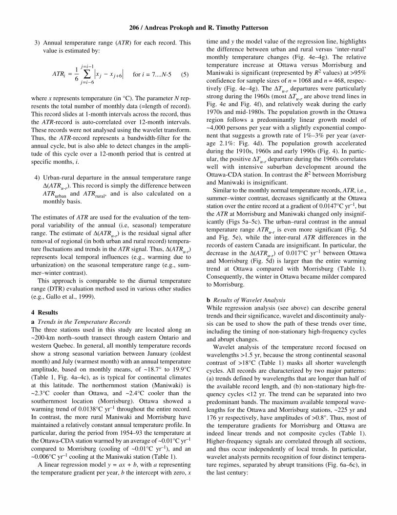
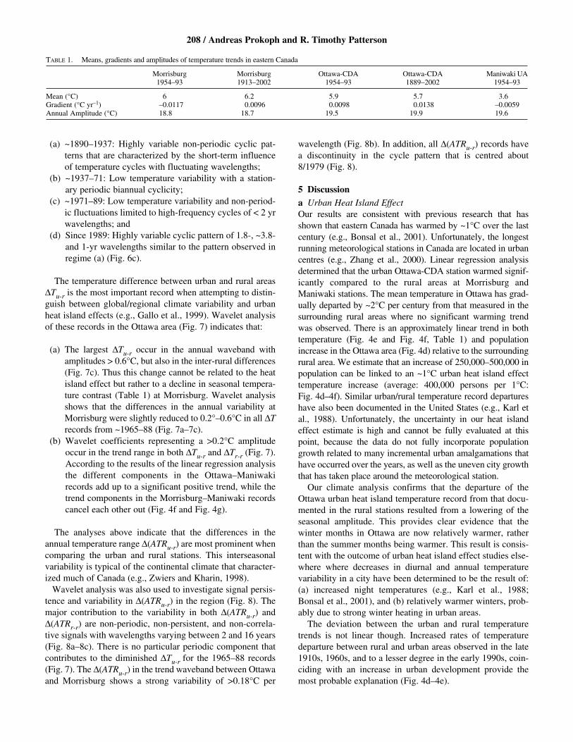
4 Resultsa Trends in the Temperature RecordsThe three stations used in this study are located along an~200-km north–south transect through eastern Ontario andwestern Quebec. In general, all monthly temperature recordsshow a strong seasonal variation between January (coldestmonth) and July (warmest month) with an annual temperatureamplitude, based on monthly means, of ~18.7° to 19.9°C(Table 1, Fig. 4a–4c), as is typical for continental climates at this latitude. The northernmost station (Maniwaki) is~2.3°C cooler than Ottawa, and ~2.4°C cooler than the southernmost location (Morrisburg). Ottawa showed a warming trend of 0.0138°C yr–1 throughout the entire record.In contrast, the more rural Maniwaki and Morrisburg havemaintained a relatively constant annual temperature profile. Inparticular, during the period from 1954–93 the temperature atthe Ottawa-CDA station warmed by an average of ~0.01°C yr–1

compared to Morrisburg (cooling of ~0.01°C yr–1), and an~0.006°C yr–1 cooling at the Maniwaki station (Table 1).

A linear regression model y = ax + b, with a representingthe temperature gradient per year, b the intercept with zero, x

time and y the model value of the regression line, highlightsthe difference between urban and rural versus ‘inter-rural’monthly temperature changes (Fig. 4e–4g). The relativetemperature increase at Ottawa versus Morrisburg andManiwaki is significant (represented by R2 values) at >95%confidence for sample sizes of n = 1068 and n = 468, respec-tively (Fig. 4e–4g). The ∆Tu-r departures were particularlystrong during the 1960s (most ∆Tu-r are above trend lines inFig. 4e and Fig. 4f), and relatively weak during the early1970s and mid-1980s. The population growth in the Ottawaregion follows a predominantly linear growth model of~4,000 persons per year with a slightly exponential compo-nent that suggests a growth rate of 1%–3% per year (aver-age 2.1%: Fig. 4d). The population growth acceleratedduring the 1910s, 1960s and early 1990s (Fig. 4). In partic-ular, the positive ∆Tu-r departure during the 1960s correlateswell with intensive suburban development around theOttawa-CDA station. In contrast the R2 between Morrisburgand Maniwaki is insignificant.

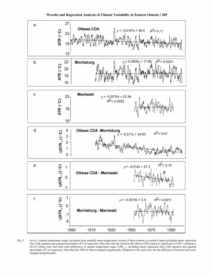
Similar to the monthly normal temperature records, ATR, i.e.,summer–winter contrast, decreases significantly at the Ottawastation over the entire record at a gradient of 0.0147°C yr–1, butthe ATR at Morrisburg and Maniwaki changed only insignif-icantly (Figs 5a–5c). The urban–rural contrast in the annualtemperature range ATRu-r is even more significant (Fig. 5dand Fig. 5e), while the inter-rural ATR differences in therecords of eastern Canada are insignificant. In particular, thedecrease in the ∆(ATRu-r) of 0.017°C yr–1 between Ottawaand Morrisburg (Fig. 5d) is larger than the entire warmingtrend at Ottawa compared with Morrisburg (Table 1).Consequently, the winter in Ottawa became milder comparedto Morrisburg.

b Results of Wavelet AnalysisWhile regression analysis (see above) can describe generaltrends and their significance, wavelet and discontinuity analy-sis can be used to show the path of these trends over time,including the timing of non-stationary high-frequency cyclesand abrupt changes.

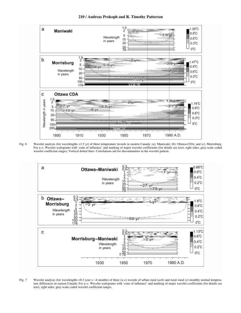
Wavelet analysis of the temperature record focused onwavelengths >1.5 yr, because the strong continental seasonalcontrast of >18°C (Table 1) masks all shorter wavelengthcycles. All records are characterized by two major patterns:(a) trends defined by wavelengths that are longer than half ofthe available record length, and (b) non-stationary high-fre-quency cycles <12 yr. The trend can be separated into twopredominant bands. The maximum available temporal wave-lengths for the Ottawa and Morrisburg stations, ~225 yr and176 yr respectively, have amplitudes of >0.8°. Thus, most ofthe temperature gradients for Morrisburg and Ottawa areindeed linear trends and not composite cycles (Table 1).Higher-frequency signals are correlated through all sections,and thus occur independently of local trends. In particular,wavelet analysts permits recognition of four distinct tempera-ture regimes, separated by abrupt transitions (Fig. 6a–6c), inthe last century:


ATR x xi j jj i

j i

= − += −

= −

∑1

6 66

1


Fig. 4 (a)–(c): Monthly mean temperature records of three stations in eastern Canada with 12-month running means, note the strong seasonal variabilitywhich is much stronger than the longer-term variability; (d): Population of Ottawa Central (solid line) at 16 counts (black triangles). Lower dashedline marks residues of an exponential growth model (scale on left) and upper straight dashed line shows linear growth model (scale on right); (e)–(g):temperature difference records between urban and rural and between rural areas, and linear regression lines with equation and squared uncertainty ofregression. Grey shaded boxes mark intervals of increased rate of population growth for correlation with the temperature difference records.

a

b

c

d

e

f

g

(a) ~1890–1937: Highly variable non-periodic cyclic pat-terns that are characterized by the short-term influenceof temperature cycles with fluctuating wavelengths;

(b) ~1937–71: Low temperature variability with a station-ary periodic biannual cyclicity;

(c) ~1971–89: Low temperature variability and non-period-ic fluctuations limited to high-frequency cycles of < 2 yrwavelengths; and

(d) Since 1989: Highly variable cyclic pattern of 1.8-, ~3.8-and 1-yr wavelengths similar to the pattern observed inregime (a) (Fig. 6c).

The temperature difference between urban and rural areas∆Tu-r is the most important record when attempting to distin-guish between global/regional climate variability and urbanheat island effects (e.g., Gallo et al., 1999). Wavelet analysisof these records in the Ottawa area (Fig. 7) indicates that:

(a) The largest ∆Tu-r occur in the annual waveband withamplitudes > 0.6°C, but also in the inter-rural differences(Fig. 7c). Thus this change cannot be related to the heatisland effect but rather to a decline in seasonal tempera-ture contrast (Table 1) at Morrisburg. Wavelet analysisshows that the differences in the annual variability atMorrisburg were slightly reduced to 0.2°–0.6°C in all ∆Trecords from ~1965–88 (Fig. 7a–7c).

(b) Wavelet coefficients representing a >0.2°C amplitudeoccur in the trend range in both ∆Tu-r and ∆Tr-r (Fig. 7).According to the results of the linear regression analysisthe different components in the Ottawa–Maniwakirecords add up to a significant positive trend, while thetrend components in the Morrisburg–Maniwaki recordscancel each other out (Fig. 4f and Fig. 4g).

The analyses above indicate that the differences in theannual temperature range ∆(ATRu-r) are most prominent whencomparing the urban and rural stations. This interseasonalvariability is typical of the continental climate that character-ized much of Canada (e.g., Zwiers and Kharin, 1998).

Wavelet analysis was also used to investigate signal persis-tence and variability in ∆(ATRu-r) in the region (Fig. 8). Themajor contribution to the variability in both ∆(ATRu-r) and∆(ATRr-r) are non-periodic, non-persistent, and non-correla-tive signals with wavelengths varying between 2 and 16 years (Fig. 8a–8c). There is no particular periodic component thatcontributes to the diminished ∆Tu-r for the 1965–88 records(Fig. 7). The ∆(ATRu-r) in the trend waveband between Ottawaand Morrisburg shows a strong variability of >0.18°C per

wavelength (Fig. 8b). In addition, all ∆(ATRu-r) records havea discontinuity in the cycle pattern that is centred about8/1979 (Fig. 8).

5 Discussiona Urban Heat Island EffectOur results are consistent with previous research that hasshown that eastern Canada has warmed by ~1°C over the lastcentury (e.g., Bonsal et al., 2001). Unfortunately, the longestrunning meteorological stations in Canada are located in urbancentres (e.g., Zhang et al., 2000). Linear regression analysisdetermined that the urban Ottawa-CDA station warmed signif-icantly compared to the rural areas at Morrisburg andManiwaki stations. The mean temperature in Ottawa has grad-ually departed by ~2°C per century from that measured in thesurrounding rural areas where no significant warming trendwas observed. There is an approximately linear trend in bothtemperature (Fig. 4e and Fig. 4f, Table 1) and populationincrease in the Ottawa area (Fig. 4d) relative to the surroundingrural area. We estimate that an increase of 250,000–500,000 inpopulation can be linked to an ~1°C urban heat island effecttemperature increase (average: 400,000 persons per 1°C: Fig. 4d–4f). Similar urban/rural temperature record departureshave also been documented in the United States (e.g., Karl etal., 1988). Unfortunately, the uncertainty in our heat islandeffect estimate is high and cannot be fully evaluated at thispoint, because the data do not fully incorporate populationgrowth related to many incremental urban amalgamations thathave occurred over the years, as well as the uneven city growththat has taken place around the meteorological station.

Our climate analysis confirms that the departure of theOttawa urban heat island temperature record from that docu-mented in the rural stations resulted from a lowering of theseasonal amplitude. This provides clear evidence that thewinter months in Ottawa are now relatively warmer, ratherthan the summer months being warmer. This result is consis-tent with the outcome of urban heat island effect studies else-where where decreases in diurnal and annual temperaturevariability in a city have been determined to be the result of:(a) increased night temperatures (e.g., Karl et al., 1988;Bonsal et al., 2001), and (b) relatively warmer winters, prob-ably due to strong winter heating in urban areas.

The deviation between the urban and rural temperaturetrends is not linear though. Increased rates of temperaturedeparture between rural and urban areas observed in the late1910s, 1960s, and to a lesser degree in the early 1990s, coin-ciding with an increase in urban development provide themost probable explanation (Fig. 4d–4e).


TABLE 1. Means, gradients and amplitudes of temperature trends in eastern Canada

Morrisburg Morrisburg Ottawa-CDA Ottawa-CDA Maniwaki UA1954–93 1913–2002 1954–93 1889–2002 1954–93

Mean (°C) 6 6.2 5.9 5.7 3.6Gradient (°C yr–1) –0.0117 0.0096 0.0098 0.0138 –0.0059Annual Amplitude (°C) 18.8 18.7 19.5 19.9 19.6


Fig. 5 (a)–(c): Annual temperature range calculated from monthly mean temperature records of three stations in eastern Canada including linear regressionlines with equation and squared uncertainty (R2) of regression. Note that only the trend for the Ottawa-CDA station is significant at >95% confidence;(d)–(f) Urban–rural and rural–rural differences in annual temperature range (ATRu-r), including linear regression lines with equation and squareduncertainty (R2) of regression. Note that the ATR for Ottawa dropped significantly compared to the rural areas but the differences between rural areaschanged insignificantly.

a

b

c

d

e

f


Fig. 6 Wavelet analysis (for wavelengths >1.5 yr) of three temperature records in eastern Canada: (a): Maniwaki; (b): Ottawa-CDA; and (c): Morrisburg.For a–c: Wavelet scalograms with ‘cone of influence’ and marking of major wavelet coefficients (for details see text), right sides: grey-scale codedwavelet coefficient ranges; Vertical dotted lines: Correlations aid for discontinuities in the wavelet pattern.

Fig. 7 Wavelet analysis (for wavelengths >0.3 year = ~4 months) of three (a–c) records of urban–rural (a+b) and rural–rural (c) monthly normal tempera-ture differences in eastern Canada: For a–c: Wavelet scalograms with ‘cone of influence’ and marking of major wavelet coefficients (for details seetext), right sides: grey-scale coded wavelet coefficient ranges.

a

b

c

a

c

b

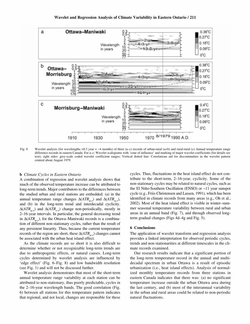
b Climate Cycles in Eastern OntarioA combination of regression and wavelet analysis shows thatmuch of the observed temperature increase can be attributed tolong-term trends. Major contributors to the differences betweenthe studied urban and rural stations are embedded: (a) in theannual temperature range changes ∆(ATRu-r) and ∆(ATRu-r),and (b) in the long-term trend and interdecadal cyclicity.∆(ATRu-r) and ∆(ATRr-r) change non-periodically, mostly in2–16-year intervals. In particular, the general decreasing trendin ∆(ATRu-r), for the Ottawa–Maniwaki records is a combina-tion of different non-stationary cycles, rather than the result ofany persistent linearity. Thus, because the current temperaturerecords of the region are short, these ∆(ATRu-r) changes cannotbe associated with the urban heat island effect.

As the climate records are so short it is also difficult todetermine whether or not recognizable long-term trends aredue to anthropogenic effects, or natural causes. Long-termcycles determined by wavelet analysis are influenced by‘edge effect’ (Fig. 6–Fig. 8) and low bandwidth resolution(see Fig. 1) and will not be discussed further.

Wavelet analysis demonstrates that most of the short-termannual temperature range variability at each station can beattributed to non-stationary, thus poorly predictable, cycles inthe 2–16-year wavelength bands. The good correlation (Fig.6) between all stations for this temperature pattern indicatesthat regional, and not local, changes are responsible for these

cycles. Thus, fluctuations in the heat island effect do not con-tribute to the short-term, 2–16-year, cyclicity. Some of thenon-stationary cycles may be related to natural cycles, such asthe El Niño-Southern Oscillation (ENSO) or ~11 year sunspotcycle (e.g., Friis-Christensen and Lassen, 1991), which has beenidentified in climate records from many areas (e.g., Oh et al.,2002). Most of the heat island effect is visible in winter–sum-mer seasonal temperature variability between rural and urbanareas in an annual band (Fig. 7), and through observed long-term gradual changes (Figs 4d–4g and Fig. 5).

6 ConclusionsThe application of wavelet transform and regression analysisprovides a linked interpretation for observed periodic cycles,trends and non-stationarities at different timescales in the cli-mate records examined.

Our research results indicate that a significant portion ofthe long-term temperature record in the annual and multi-decadal spectrum in urban Ottawa is a result of episodicurbanization (i.e., heat island effects). Analysis of normal-ized monthly temperature records from three stations ineastern Canada indicates that there was: (a) no significanttemperature increase outside the urban Ottawa area duringthe last century, and (b) most of the interannual variabilityin the urban and rural areas could be related to non-periodicnatural fluctuations.


Fig. 8 Wavelet analysis (for wavelengths >0.3 year = ~4 months) of three (a–c) records of urban-rural (a+b) and rural-rural (c) Annual temperature rangedifference records in eastern Canada: For a–c: Wavelet scalograms with ‘cone of influence’ and marking of major wavelet coefficients (for details seetext), right sides: grey-scale coded wavelet coefficient ranges; Vertical dotted line: Correlations aid for discontinuities in the wavelet pattern centred about August 1979.

a

b

c


ReferencesAPPENZELLER, C.; T.F. STOCKER and M. ANKLIN. 1998. North Atlantic oscilla-

tion dynamics recorded in Greenland ice cores. Science, 282: 446–449.BONSAL, B.R.; X. ZHANG, L.A. VINCENT and W.D. HOGG. 2001. Characteristics of

daily and extreme temperatures over Canada. J. Clim. 14: 1959–1976.BUNDE, A; S. HAVLIN, E. KOSCIELNY-BUNDE and H.-J. SCHELLNHUBER. 2001.

Long-term persistence in the atmosphere: Global laws and tests of climatemodels. Physica A: Stat. Mech. Apps. 302: 255–267.

CARSLAW, K.S.; R.G. HARRISON and J. KIRKBY. 2002. Cosmic rays, clouds, andclimate. Science, 298: 1732–1737.

CHAO, B.F. and I. NAITO. 1995. Wavelet analysis provides a new tool for study-ing Earth’s rotation. EOS 76: 161–165.

DAUBECHIES, I. 1992. Ten lectures on wavelets. CBMS-NSF RegionalConference Series in Applied Mathematics, No. 61, SIAM Press,Philadelphia, 357 pp.

FRIIS-CHRISTENSEN, E. and K. LASSEN. 1991. Length of the solar cycle: An indi-cator of solar activity closely associated with climate. Science, 254: 698–700.

GALLO, K.P.; D.R. EASTERLING and T.C. PETERSON. 1996. The influence of landuse/land cover on climatological values in the diurnal temperature range.J. Clim. 9: 2941–2944.

———; T.W. OWEN, D.R. EASTERLING and P.F. JAMASON. 1999. Temperaturetrends of the U.S. Historical Climatology Network based on satellite-des-ignated land use/land cover. J. Clim. 12: 1344–1348.

GEDALOF, Z. and D.J. SMITH. 2001. Interdecadal climate variability and regime-scale shifts in Pacific North America. Geophys. Res. Lett. 28:1515–1518.

GROSSMAN, A. and J. MORLET. 1984. Decomposition of Hardy functions intosquare integrable wavelets of constant shape. SIAM J. Math. Anal. 15:732–736.

IPCC. 1996. Climate change 1995: The science of climate change. In:Intergovernmental Panel on Climate Change. J.T. Houghton, L.G. MiroFilho, B.A. Callander, N. Harris, A. Kattenberg and K. Maskell (Eds),Cambridge University Press, Cambridge. 572 pp.

KAISER, G. 1993. A friendly guide to wavelets. Birkenhaeuser Verlag, Basel,300 pp.

KARL, T.R.; R.R. HEIM JR. and R.G. QUAYLE. 1991. The greenhouse effect incentral north America: If not now, when? Science, 251: 1058–1061.

———; H.F. DIAZ and G. KUKLA. 1988. Urbanization: Its detection and effectin the United States climate record. J. Clim. 1: 1099–1123.

KATZ, R.W. 1988. Statistical procedures for making inferences about climatevariability. J. Clim. 1: 1057–1064.

LUCERO, O.A. and N.C. RODRIGUEZ. 2000. Statistical characteristics of inter-decadal fluctuations in the Southern Oscillation and the surface tempera-ture of the equatorial Pacific. Atmos. Res. 54: 87–104.

MORLET, J.; G. AREHS, I, FOURGEAU and D. GIARD. 1982. Wave propagation andsampling theory. Geophys. 47: 203.

NAKKEN, M. 1999. Wavelet analysis of rainfall-runoff variability isolating cli-matic from anthropogenic patterns. Environ. Modelling Software 14:283–295.

OH, H-S.; C.M. AMMANN, P. NAVEAU, D. NYCHKA and B.L. OTTO-BLIESNER. 2002.Muli-resolution time series analysis applied to solar irradiance and climatereconstructions. J. Atmos. Solar-Terr. Phys. 65: 191–201.

OKE, T.R. 1982. The energetic basis of the urban heat island. Q. J. R.Meteorol. Soc. 108: 1–24.

PROKOPH, A. and F. BARTHELMES. 1996. Detection of nonstationarities in geo-logical time series: Wavelet transform of chaotic and cyclic sequences.Comput. Geosci. 22: 1097–1108.

QUEREDA SALA, J.; A. GIL OLCINA, A. PEREZ-CUEVAS, J. OLCINA-CANTOS, A. RICO

AMOROS and E. MONTON CHIVA. 2000. Climate warming in the SpanishMediterranean: Natural trend or urban effect. Clim. Change, 46: 473–483.

RIOUL, O. and M. VETTERLI. 1991. Wavelets and signal processing. IEEESpecial Mag. pp. 14–38.

TORRENCE, C. and G.P. COMPO. 1998. A Practical guide to wavelet analysis:Bull. Am. Meteorol. Soc. 79: 61–78.

VINCENT, L.A. 1998. A technique for the identification of inhomogeneities inCanadian temperature series. J. Clim. 11: 1094–1104.

WARE, D.M. and R.E. THOMSON. 2000. Interannual to multidecadal timescaleclimate variations in the northeast Pacific. J. Clim. 13: 3209–3220.

ZHANG, X. L.A. VINCENT, W.D. HOGG and A. NIITSOO. 2000. Temperature andprecipitation trends in Canada during the 20th century. ATMOSPHERE-OCEAN, 38: 395–429.

ZWIERS, F.W. and V.V. KHARIN. 1998. Intercomparison of interannual variabil-ity and potential predictability: An AMIP diagnostic project. Clim. Dyn.14: 517–528.

Documents

Application of Wavelet and Regression Analysis in Assessing Temporal and Geographic Climate