APPLICATION OF VISCOELASTIC, VISCOPLASTIC, AND RATE-AND-STATE FRICTION CONSTITUTIVE LAWS TO THE DEFORMATION OF UNCONSOLIDATED SANDS

A DISSERTATION

SUBMITTED TO THE DEPARTMENT OF GEOPHYSICS

AND THE COMMITTEE ON GRADUATE STUDIES

OF STANFORD UNIVERSITY

IN PARTIAL FULFILLMENT OF THE REQUIREMENTS

FOR THE DEGREE OF

DOCTOR OF PHILOSOPHY

Paul N. Hagin

December 2003

ii

„ Copyright by Paul Hagin 2004All Rights Reserved

iv

ABSTRACT

Laboratory experiments on dry, unconsolidated sands from the Wilmington field, CA,

reveal significant viscous creep strain under a variety of loading conditions. In

hydrostatic compression tests between 10 and 50 MPa of pressure, the creep strain

exceeds the magnitude of the instantaneous strain and follows a power law function of

time. Interestingly, the viscous effects only appear when loading a sample beyond its

preconsolidation pressure. Cyclic loading tests (at quasi-static frequencies of 10-6 to 10-2

Hz) show that the bulk modulus increases by a factor of two with increasing frequency

while attenuation remains constant. I attempt to fit these observations using three classes

of models: linear viscoelastic, viscoplastic, and rate-and-state friction models. For the

linear viscoelastic modeling, I investigated two types of models; spring-dashpot

(exponential) and power law models. I find that a combined power law-Maxwell solid

creep model adequately fits all of the data. Extrapolating the power law-Maxwell creep

model out to 30 years (to simulate the lifetime of a reservoir) predicts that the static bulk

modulus is 25% of the dynamic modulus, in good agreement with field observations.

Laboratory studies also reveal that a large portion of the deformation is permanent,

suggesting that an elastic-plastic model is appropriate. However, because the viscous

component of deformation is significant, an elastic-viscoplastic model is necessary. An

appropriate model for unconsolidated sands is developed by incorporating Perzyna

(power law) viscoplasticity theory into the modified Cambridge clay cap model.

Hydrostatic compression tests conducted as a function of volumetric strain rate produced

values for the required model parameters. As a result, by using an end cap model

combined with power law viscoplasticity theory, changes in porosity in both the elastic

and viscoplastic regimes can be predicted as a function of both stress path and strain rate.

To test whether rate-and-state friction laws can be used to model creep strain, I expand

the rate-and-state formulation to include deformation under hydrostatic stress boundary

conditions. Results show that the expanded rate-and-state formulation successfully

describes the creep strain of unconsolidated sand. Finally, I show that the viscoplastic end

cap and rate-and-state models are mathematically similar.

v

PREFACE

This dissertation is primarily about the mechanics of unconsolidated sands. A

great body of literature already exists on the mechanics of soils and clays, stemming from

the environmental and civil engineering literature. On the other end of the diagenetic

spectrum, the mechanics of cemented sandstones is well understood, thanks to several

decades of rock mechanics and rock physics research. However, not much data is

available to those working in areas such as reservoir and aquifer geomechanics, where

unconsolidated, uncemented sands can exist at depths of several kilometers and tens of

megaPascals of pressure.

A significant portion of the hydrocarbon reserves in the United States exists in

unconsolidated sand reservoirs offshore California and in the deepwater Gulf of Mexico.

Producing these reserves has proved to be complicated in some cases, for example in the

Wilmington Field in California, due to significant subsidence (~10 m vertical subsidence)

associated with production was observed, but not expected. Similar subsidence has been

observed in the San Joaquin valley due to excessive pumping of water from local aquifers

for irrigation. Water and steam flooding largely solved the subsidence problems at

Wilmington, but the solution came too slowly; piers and marinas were forced to relocate,

train tracks and oil wells were sheared apart, and several small earthquakes occurred due

to the subsidence. Obviously, if the mechanics of unconsolidated sands at high pressures

was better understood at the time, the subsidence might have been predicted and taken

into account by reservoir engineers.

A series of laboratory experiments was conducted on sand from the Wilmington

field and several synthetic sands, with the goal of finding an appropriate constitutive law

which could be used to predict subsidence and porosity loss in reservoirs and aquifers.

All of the samples were washed with solvents and dried under vacuum prior to testing, in

order to ensure that the dry frame properties, and not the combined effects of grains and

pore fluids, were measured during the experiments. All of the tests were carried out on a

conventional triaxial loading frame, with both hydrostatic pressure and triaxial stress

boundary conditions available.

vi

The results from these experiments are described in Chapter 1. The most

significant finding is simply that a large component of the deformation is viscous; in fact,

the viscous deformation is the same order of magnitude as the elastic deformation above

10 MPa in pressure. The viscous deformation occurs as creep strain and is time-

dependent. As the simplest way to describe deformation with a time-dependent

component is through viscoelasticity theory, experiments were conducted in the

frequency domain to test whether the samples appeared to be qualitatively viscoelastic.

The results from these experiments confirm that unconsolidated sands can be treated as

viscoelastic, at least during loading. In addition, the static bulk modulus was observed to

increase by a factor of 2 as loading frequency was increased from 10-6 to 10-3 per second.

Modeling the deformation of unconsolidated sands using viscoelastic constitutive

laws is discussed in more detail in Chapter 2. Several different pedagogical spring-and-

dashpot models are examined in relation to available creep strain, modulus dispersion,

and attenuation data. Choosing a “successful” model here is partly determined by the

number of free parameters and complexity of the model; the idea is to find a simple

model that could be used to make a back-of-the-envelope calculation to predict the

compaction in a producing reservoir over a certain number of years. Each of the models

is forced to fit the creep strain data by solving for the free parameters using a least-

squares approach. These parameters are then used to try to model the observed modulus

dispersion and attenuation. Results from this procedure indicate that any of the models is

capable of describing the creep strain data, but only a combined Maxwell solid-power

law model succeeds in modeling all of the available data.

Observations of long-duration creep strain tests show that the majority of the

compaction is irreversible. This leads to Chapter 3, which explores the application of

viscoplastic models to the mechanics of unconsolidated sands. The chapter begins with a

brief review of the modified Cambridge clay end cap model, an elastic-plastic model that

includes plastic failure under hydrostatic conditions as well as shear. This model is

relatively simple in terms of free parameters, but it has been shown to describe the

deformation of sands and clays under a wide variety of loading conditions. The one thing

it lacks is the capability to model time-dependent strain, but that can be built in via

Perzyna viscoplasticity theory. Perzyna proposed a power law relationship between strain

vii

rate and stress in viscoplastic materials. It is used here because it is relatively easy to

integrate with the modified Cam clay model, and because it has been successfully used to

model unconsolidated materials in the literature. Nearly all of the free parameters can be

solved for using the results of hydrostatic compaction experiments under strain rate

feedback control. The modified Cam clay viscoplastic model is shown to successfully

describe the deformation of unconsolidated Wilmington sand. This model is a better

match to the data than the viscoelastic models in Chapter 2 because it works for both

loading and unloading conditions.

Shifting gears rather abruptly, viscoelastic and viscoplastic models are abandoned

the rate-and-state friction model in Chapter 4. The time-dependent compaction observed

in Wilmington sand under hydrostatic pressure looks qualitatively similar to the time-

dependent compaction occurring under normal stress during holds in a typical slide-hold

test. It therefore seems intuitively possible that the rate-and-state equation for compaction

of a gouge layer during a hold might also describe the compaction of sand under

hydrostatic pressure. As rate-and-state experiments are typically conducted using a

double-direct shear apparatus, a change in boundary conditions needs to occur before the

rate-and-state equations can be applied to hydrostatic compaction. This change in

boundary conditions is accommodated by writing the rate-and-state compaction equation

in terms of invariants.

Appropriate stress and strain invariants are found by ensuring that engineering

shear strain, normal compaction, and Poisson’s ratio are recovered for double direct shear

boundary conditions. Completing the analysis reveals that the rate-and-state equation can

be used to model the creep compaction of unconsolidated sands. Solving for the free

parameters in the model of Wilmington sand under hydrostatic conditions results in

values equal to those recovered when modeling the normal compaction of quartz gouge

under direct shear conditions. This result suggests that the rate-and-state friction equation

might be used to simultaneously model the compaction in a producing reservoir and any

associated slip on nearby faults.

Chapter 3 showed that hydrostatic creep compaction of unconsolidated sand can

be modeled using viscoplasticity theory in the form of a rate-dependent end cap. Chapter

4 showed that hydrostatic creep compaction of unconsolidated sand can also be modeled

viii

using rate-and-state friction. Both models have a rate component and a state component,

although these are described in different ways. Since both models are capable of fitting

the creep strain of unconsolidated sand and they are qualitatively similar, it seems logical

(at least to me) that they might be mathematically equivalent. This possibility is explored

in Chapter 5. As in Chapter 4, since the two models exist in different stress spaces,

writing each model in terms of stress and strain invariants in required in order to compare

them. The modified Cam clay viscoplastic model is easily written in terms of J1, and J2D,

the first invariant of the stress tensor, and the second invariant of the deviatoric stress

tensor, respectively. Writing the rate-and-state equation in terms of invariants is more

complicated, but can be done, and it conveniently turns out that J1 and J2D are correct in

this case too. Rigorous proofs are abandoned for brevity and common sense.

Next, some assumptions need to be made, because rate-and-state experiments

typically monitor friction and state as a function of strain rate, while viscoplastic end cap

tests typically monitor failure pressure and porosity as a function of strain rate. Assuming

that state is equivalent to porosity, and that state is constant, allows for a meaningful

comparison of the two models. The completed analysis indicates that the two models are

equivalent, given the previously stated assumptions. This finding is very interesting given

that the end cap model was developed to describe the deformation of soils subjected to

very small stresses, while the rate-and-state friction model was developed to describe the

changes in dynamic friction occurring between granite blocks under very large stresses.

The implication for the similarity between the two models is that each model is

describing part of a more fundamental underlying physical process that remains to be

found experimentally.

A few words about how to read this dissertation

I tried to arrange the chapters in terms of relevance and complexity. The

experiments are pretty straight forward and are the most significant part of this project, so

they are described first. The three theory chapters are arranged from most simple to most

complex. Linear viscoelasticity theory can largely be understood through the use of

schematic diagrams, and the math is mostly Laplace transforms to go from the time

domain to the frequency domain. Elastic-plastic end cap models, particularly when rate-

ix

dependence in built in, are conceptually harder to understand, but the plasticity theory

can be ignored for the most part, and the model can be described simply using geometry.

Rate-and-state friction is even more complex, and rewriting it in terms of stress and strain

invariants is virtually ridiculous. However, all of the modeling was done for a reason,

mainly trying to understand and predict creep strain in unconsolidated sands.

Each chapter was written as an individual paper. While I recommend reading

them all in the order they are presented, each chapter should be self-contained. If you

were only to read one chapter, I would highly recommend Chapter 1, which presents the

experimental results. If you hate math, start with Chapter 1, proceed to Chapter 2, and see

how much you can stomach. Those with a modeling background in civil engineering or

soil mechanics might want to start with Chapter 3 and then read Chapter 1. Readers who

come from the school of hard rocks might want to start with Chapter 4. Chapter 5 was

written especially for people who have far too much free time or are suffering from

insomnia.

Acknowledgements

I have been here for far too long to properly thank everyone who helped me along

the way, so please do not take offense if somehow I have forgotten you. I need to start by

thanking the Stanford Rock Physics and Borehole Geophysics (SRB) consortium, who

paid my rent and provided the funding for my research for the past 6 years. Next, I need

to thank my advisor, Mark Zoback, for being my teacher, mentor, and friend. I hope that I

have been able to teach him some things along the way as well. I need to thank everyone

on my reading and exam committees for challenging me and helping to make this a better

thesis – Norm Sleep, Dave Lockner, Greg Beroza, and Ronnie Borja. I need to thank Ali

Mese, Carl Chang, Chandong Chang, and Gilbert Palafox for teaching me how to work in

the laboratory. New England Research provided me with much needed technical

assistance and a machine to crush dirt with. I want to thank my research group and my

band, Chinese Radio, for much needed emotional support. I couldn’t have made it this far

without the loving support of Cara Rice – I can’t possibly thank her enough. Finally, I

need to thank my family, who put up with my endless complaints about grad school.

x

TABLE OF CONTENTS

Abstract ivPreface/Acknowledgements v

Table of Contents x

List of Tables xiiList of Figures xiii

1. Viscous Deformation of Unconsolidated Reservoir Sands (Part 1): 1Time-dependent Deformation, Frequency Dispersion, andAttenuation

1.1 Introduction 21.2 Observations of Creep Strain 5

1.3 Generalized Viscous Deformation 10

1.4 Frequency, Pressure, and Strain-rate Effects 121.5 Discussion 17

1.6 Conclusions 19

1.7 References 201.8 Appendix A: Sample Description 21

1.9 Appendix B: Summary of Experimental Results 251.10 Appendix C: Strain-amplitude Effects 27

2. Viscous Deformation of Unconsolidated Reservoir Sands (Part II): 42Linear Viscoelastic Models2.1 Introduction 43

2.2 Summary of Observations 45

2.3 Linear Viscoelasticity Theory (Basic Concepts) 472.4 Linear Viscoelasticity Theory (Mathematical Details) 48

2.5 Modeling Creep, Dispersion, and Attenuation 562.6 Application to the Wilmington Reservoir 62

2.7 Conclusions 64

2.8 References 652.9 Appendix: Power Law and Burgers Solid Models 66

xi

3. Application of Time-Dependent End Cap Models to the 75Deformation of Unconsolidated Sands3.1 Introduction 75

3.2 Theory Part 1 – Modified Cambridge Clay Model 77

3.3 Theory Part 2 – Perzyna Viscoplasticity 803.4 Laboratory Studies and Model Verification 81

3.5 Discussion 833.6 Conclusions 84

3.7 References 85

4. Application of Rate-and-State Friction Laws to Creep 92Compaction of Unconsolidated Sand under HydrostaticLoading Conditions

4.1 Introduction 924.2 Expanding Rate-and-State Friction to Include Hydrostatic 94 Stress Boundary Conditions

4.3 Laboratory Studies and Model Verification 974.4 Discussion 100

4.5 Conclusions 1014.6 Appendix A: Representing Hydrostatic Compression 102 Using Rate-and-State Theory

4.7 Appendix B: Loading Rate Effects on the Rate-and-State 104 Parameter Ce

4.8 References 105

5. Comparing Time-Dependent End Cap and Rate-and-State 113Friction Models

5.1 Introduction 113

5.2 Theory Part 1: Time-dependent End Cap Models and 115 Stress Invariants

5.3 Theory Part 2: Rate-and-State Friction and Stress 116 Invariants

5.4 Comparing Rate/State and Time-dependent End Cap Models 119

5.5 Discussion `121

5.6 Conclusions 123

5.7 References 123

xii

LIST OF TABLES

1-1: Creep Strain Measurements 25

1-2: Stress Relaxation Tests 26

1-3: Strain-rate Effects in Triaxial Tests 27

3-1: Elastic Modulus and Elastic-Plastic Transition for 83Wilmington Sand

4-1: Compilation of Compaction Coefficients 106

xiii

LIST OF FIGURES

1-1: Creep Strain Depends on the Presence of Clay Minerals 29

1-2: Creep Strain as a Function of Pressure 30

1-3: Comparing Incremental Instantaneous and Creep Strains 31

1-4: The Majority of Creep Strain is Permanent 32

1-5: Creep Strain Follows a Power law Function of Time 33

1-6: A Review of Linear Viscoelasticity Theory 34

1-7: Bulk Modulus Dispersion Experimental Procedure 35

1-8: Bulk Modulus Dispersion Results 36

1-9: Bulk Modulus Dispersion as a Function of Pressure 37

1-10: Quasi-static Attenuation Experimental Procedure 38

1-11: Quasi-static Attenuation Results 39

1-12: Triaxial Compression Experimental Results 40

1-13: Bulk Modulus Dispersion as a Function of Strain 41 Amplitude

2-1: Common Viscoelastic Models 70

2-2: Stress Response to Constant Strain-rate Deformation 71

2-3: Modeling Creep Strain with Linear Viscoelastic Models 72

2-4: Modeling Bulk Modulus Dispersion 73

2-5: Modeling Quasi-static Attenuation 74

3-1: Comparing End Cap and Mohr-Coulomb Failure Models 87

3-2: Constructing a Time-dependent End Cap Model 88

3-3: Hydrostatic Compression Data via Volumetric Strain-rate 89 Feedback Control

3-4: Hydrostatic Compression Data (Log-Log Plot) 90

3-5: Solving for Perzyna Viscoplasticity Parameters 91

4-1: Rate-and-State Compaction Model: Wilmington Sand 107

4-2: Rate-and-State Compaction Model: Ottawa Sand 108

4-3: Rate-and-State Compaction Model: Ottawa + 10% Clay 109

4-4: Ce as a Function of Hydrostatic Pressure 110

4-5: Solving for ‘N’ in Wilmington Sand 111

xiv

4-B1: Effects of Initial Loading Rate on Ce 112

5-1: Comparing Direct Shear and Triaxial Boundary Conditios 125

5-2: Comparing Rate-and-State and Time-dependent End Cap Models 126

1

CHAPTER 1

VISCOUS DEFORMATION OF UNCONSOLIDATED RESERVOIR SANDS (PART

I): TIME-DEPENDENT DEFORMATION, FREQUENCY DISPERSION, AND

ATTENUATION

This paper was written with Mark Zoback and has been accepted by Geophysics

ABSTRACT

Laboratory experiments on dry, unconsolidated sands from the Wilmington field, CA,

reveal significant viscous creep strain under a variety of loading conditions. In hydrostatic

compression tests, following initial loading to 10 MPa, the creep strain that accompanies

5 MPa loading steps to 15, 20, 25, and 30 MPa exceeds the magnitude of the

instantaneous strain (~ 3x10-3). We observed a two-fold increase in bulk modulus with

frequency over the range of frequencies tested (10-6 to 10-2 Hz), which is consistent with

a viscoelastic rheology of unconsolidated sand. The data demonstrate that the effective

static bulk modulus is approximately one third that at seismic frequencies. By measuring

the phase-lag between stress and strain during the loading cycles, we were also able to

show that inelastic attenuation is nearly constant (Q ≈ 5) over the 4-decade range of

frequencies tested at a strain amplitude of 10-3. Interestingly, the viscous effects only

appear when loading a sample beyond its preconsolidation. Triaxial tests show that the

relationship between differential stress and axial strain is positively dependent on axial

2

strain-rate, and that unconsolidated sand continues to deform viscously even at large

strains (~7%). All experiments were conducted at room temperature and humidity. A

limited number of experiments with unconsolidated reservoir sand from the Gulf of

Mexico show similar behavior.

INTRODUCTION

During production, unconsolidated sand reservoirs are commonly observed to undergo

compaction. In most cases, this compaction is irrecoverable and therefore not predictable

using traditional poroelasticity theory (Kosloff and Scott, 1980b). In addition, the

ultimate reservoir compliance typically exceeds that predicted from elastic moduli

obtained from seismic velocities and sonic well-logs. Time- and rate-dependent

compaction is also commonly observed in unconsolidated sand reservoirs, for example in

the Wilmington field and San Joaquin Valley, CA (Kosloff and Scott, 1980a, Prokpovich,

1983) and the Bolivar coast heavy-oil fields (Schenk and Puig, 1983). Understanding the

mechanics of compaction in unconsolidated sand is important for the accurate prediction

of porosity loss in reservoirs and the potential for surface subsidence. In this study we

characterize the mechanics of compaction in several unconsolidated sand reservoirs by

conducting a series of laboratory measurements on samples obtained from the Wilmington

field in Long Beach, California.

Several previous laboratory studies of the physical properties of reservoir rocks have

shown that there is a time-dependent component of deformation. However, time-depend-

ent deformation (and the associated frequency-dependence of elastic properties) is

typically associated with pore-fluid effects and poroelasticity (Biot, 1962; Griffiths,

3

1994; Mavko and Jizba, 1991). Time- and rate- dependent moduli are also caused by grain

adhesion (Tutuncu and Sharma, 1992), and changes in contact area associated with rate

and state friction (Dieterich, 1978). However, recent laboratory studies of unconsolidated

sands have shown that time-dependent deformation may also be attributed to the viscous

behavior of clays in the solid frame (e.g., Wood, 1990, Chang et al., 1997) and the

rearrangement of grains.

Clays are known to exhibit a wide range of elastic, viscous, and plastic properties.

The degree to which any of these mechanical properties is observed in the laboratory

depends strongly upon the water content and chemistry of the clay, as well as other

conditions including the temperature, deformation rate, and loading history (e.g. Worrall,

1968, Mitchell et al., 1968, Leroueil et al., 1985). Some authors have described

observations of time-dependent deformation in undrained saturated clays using

viscoelastic and viscoplastic models (Astbury et al., 1965), while others have argued that

such observations represent the effects of an underlying thermally activated process

similar to diffusion creep (Mitchell et al., 1968). Similar studies of single biotite mica

grains (Kronenberg et al., 1990) have revealed that time-dependent deformation can occur

along basal planes due to dislocation glide, which is a thermally activated process.

However, the influence of such time-dependent processes in clays and micas on the

mechanical behavior of unconsolidated sands of mixed mineralogy has not yet been fully

described.

Several authors have studied time-dependent creep strain in the laboratory under

constant stress conditions in saturated unconsolidated sands. Ostermeier (1995) observed

4

creep strain under constant hydrostatic loading conditions in saturated Gulf of Mexico

turbidite sands and characterized his observations using a Standard Linear Solid

viscoelastic model. Dudley et al. (1994) observed similar behavior in saturated Gulf of

Mexico turbidite sands under uniaxial strain conditions and modeled the creep strain using

a power law function of time. Yale et al. (1993) observed creep strain in the form of

stress-rate effects in compaction experiments on unconsolidated sands.

In an effort to isolate the behavior of the solid frame from that of the pore fluid in

saturated samples, Chang et al. (1997) conducted laboratory experiments on room-dry

unconsolidated sands. They found creep strain in room-dry samples, which suggested

that creep strain in unconsolidated sands is an intrinsic property of the solid frame.

Furthermore, they demonstrated an increase of bulk modulus with increasing loading

frequency at frequencies between 10-5 and 10-3 Hz, and modeled both the creep strain and

the low-frequency modulus dispersion using a Standard Linear Solid viscoelastic model.

In this paper, we present the results from a comprehensive series of hydrostatic

loading experiments on unconsolidated sands under room-dry conditions. The

experiments were designed to explore the effects of pressure, strain-amplitude, loading

history, and loading frequency on creep strain, bulk modulus, and attenuation. We also

investigate the effect of axial strain rate on differential stress and Young’s modulus in a

series of triaxial tests. In Chapter 2 we utilize the experimental data in the context of

linear viscoelasticity theory to arrive at a constitutive law which best describes the

behavior of unconsolidated reservoir sands.

5

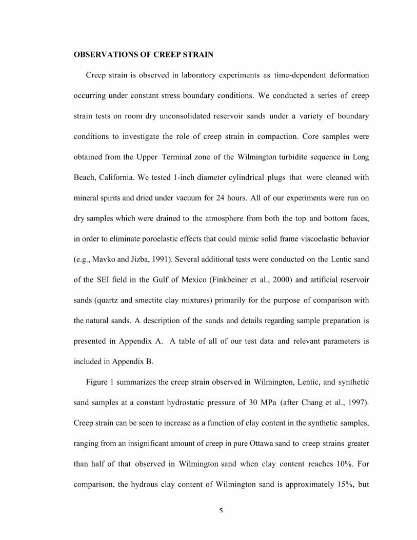
OBSERVATIONS OF CREEP STRAIN

Creep strain is observed in laboratory experiments as time-dependent deformation

occurring under constant stress boundary conditions. We conducted a series of creep

strain tests on room dry unconsolidated reservoir sands under a variety of boundary

conditions to investigate the role of creep strain in compaction. Core samples were

obtained from the Upper Terminal zone of the Wilmington turbidite sequence in Long

Beach, California. We tested 1-inch diameter cylindrical plugs that were cleaned with

mineral spirits and dried under vacuum for 24 hours. All of our experiments were run on

dry samples which were drained to the atmosphere from both the top and bottom faces,

in order to eliminate poroelastic effects that could mimic solid frame viscoelastic behavior

(e.g., Mavko and Jizba, 1991). Several additional tests were conducted on the Lentic sand

of the SEI field in the Gulf of Mexico (Finkbeiner et al., 2000) and artificial reservoir

sands (quartz and smectite clay mixtures) primarily for the purpose of comparison with

the natural sands. A description of the sands and details regarding sample preparation is

presented in Appendix A. A table of all of our test data and relevant parameters is

included in Appendix B.

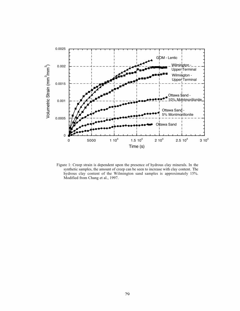
Figure 1 summarizes the creep strain observed in Wilmington, Lentic, and synthetic

sand samples at a constant hydrostatic pressure of 30 MPa (after Chang et al., 1997).

Creep strain can be seen to increase as a function of clay content in the synthetic samples,

ranging from an insignificant amount of creep in pure Ottawa sand to creep strains greater

than half of that observed in Wilmington sand when clay content reaches 10%. For

comparison, the hydrous clay content of Wilmington sand is approximately 15%, but

6

Wilmington sand also contains other ductile minerals such as biotite mica. The Lentic sand

contains only traces of clay minerals, but the mean grain size is an order of magnitude less

than that of Wilmington and Ottawa sand. Creep strain in the Lentic and Wilmington

sands are the same order of magnitude after six hours. These observations suggest that

grain rearrangement facilitated by the presence of clays and other ductile minerals is the

physical mechanism responsible for creep strain in unconsolidated reservoir sands.

In order to investigate the effects of stress magnitude on creep strain, we conducted

step loaded hydrostatic pressure experiments on the Wilmington sand. Because creep

strain will continue indefinitely under constant stress boundary conditions, it is important

to unload the sample before initiating subsequent step increases in stress. Otherwise, it is

very difficult to distinguish the effects of each new stress step. Figure 2 shows a typical

experiment. The sample is first loaded to 10 MPa at a rate of 10 MPa/hr, followed by 6

hours of constant pressure during which time creep strain is observed, then unloaded to 5

MPa at 10 MPa/hr before increasing the pressure to 15 MPa. This pattern of loading to a

given pressure, maintaining constant pressure to observe creep, unloading to half of the

given pressure, and then increasing the given pressure by an increment of 5 MPa is

continued until a maximum pressure of 30 MPa is reached, at which point the test is

stopped arbitrarily.

These tests on dry Wilmington sand indicate that the instantaneous (incorporating

both elastic and plastic deformation) and viscous components of deformation occur simul-

taneously. However, if the loading rate is fast enough, in this case greater than 10 MPa/hr,

the instantaneous and viscous components of deformation can largely be distinguished, as

7

indicated in Figure 2. Separating the instantaneous and viscous components of

deformation allows for the determination of the relative contribution of each.

Figure 3 compares the instantaneous and creep strains plotted as both incremental and

cumulative functions of pressure. In Figure 3a, the strains which occurred with each 5

MPa step increase in pressure are plotted. In Figure 3b the cumulative instantaneous

strain up to a given pressure is shown. The creep strain data plotted is the creep strain

which accumulated after 6 hours, the length of the hold time during the pressure cycling

experiments. The instantaneous strain decreases with increasing pressure, indicating that

the sample is hardening with pressure as porosity decreases, as expected. However, the

incremental creep strain remains constant with increasing confining pressure, and is

greater in magnitude than the instantaneous strain above 15 MPa. In other words, above

15 MPa hydrostatic pressure, more than half of the deformation is due to creep strain.

Note that the creep strain is linear as a function of pressure, even though it is non-linear in

time, because the creep strain increment is constant as a function of pressure increment.

Figure 3b shows the cumulative instantaneous volumetric strain as a function of

increasing pressure, which can be interpreted like a stress-strain curve. The figure

represents a compilation of data from tests that follow the same type of procedure shown

in Figure 2. Refer to the table in Appendix B for details. These data can be empirically fit

with a power law of the form e(Pc)=B*Pcn, where e is volumetric strain, Pc is the

confining pressure, B has a value of 0.0083, and n = 0.54. Note that this equation is only

valid during loading, and includes both elastic and plastic deformation.

8

In order to develop a constitutive law for unconsolidated sands that enables a more

accurate prediction of compaction in reservoirs, it is desirable to distinguish not only

between instantaneous and viscous deformation, but also between the elastic and plastic

components of the instantaneous deformation. We investigated the nature of the

instantaneous component of deformation by conducting long-term creep tests to reduce

the effects of continued viscous flow in the sample. We also compared the creep strain

during initial loading with that which occurred during unloading/reloading. A typical

experiment on dry Wilmington sand is shown in Figure 4. The test begins by loading the

sample to some small hydrostatic pressure to seat the sample and then increasing the

initial load to the test pressure quickly. For the test depicted in Figure 4, a pressure of 30

MPa was applied in one minute. The pressure is then held constant for 5 days, and creep

strain is observed. After 5 days of hold time, the sample is unloaded to a lower pressure

and held constant for several days to observe viscoelastic recovery, or the lack thereof.

The sample is then partially reloaded to an intermediate pressure and held constant for

several hours to allow for the observation of creep strain, after which the sample is

unloaded completely.

Several things can be seen in Figure 4. The most striking is that the majority of the

deformation is irrecoverable. Initially loading the sample to 30 MPa of pressure produces

a volumetric strain of almost 5%, but only 0.7% volumetric strain is recovered during un-

loading. In other words, nearly 85% of the deformation that occurred during initial loading

to 30 MPa was irrecoverable. Note that while there is a significant viscous component of

deformation following initial loading, the response to unloading appears to be elastic.

9

Reloading the sample to a pressure of 10 MPa also appears to be elastic; no creep strain

was observed following reloading. Based on the observations, the viscous component of

deformation only contributes to the initial loading behavior of unconsolidated sands.

During unloading and reloading, unconsolidated sands behave elastically. Given the

complexity of deformational styles seen under just simple hydrostatic loading conditions,

it is obvious that it might be difficult to predict the behavior of these sands under

different boundary conditions. As we show in the next section, this is precisely why

choosing an appropriate model is so important.

Focusing on the creep strain portion of the test shown in Figure 4, notice again that

creep strain is highly non-linear as a function of time. The majority of the deformation

occurs during the first ten hours, but creep strain continues at a decreasing rate throughout

the entire 140 hours of observation time. After 100 hours, the creep strain appears to be

approaching a limit, which suggests that the sample may be reaching an equilibrium state.

However, plotting the same data in log-log space (see Figure 5) indicates that the creep

strain follows a power law function of time, indicating that creep strain will continue in

the sample indefinitely, but at slower and slower rates. Longer observation times are

needed to determine whether or not creep strain continues indefinitely in unconsolidated

sands.

In summary, observations of creep strain in room-dry unconsolidated reservoir sands

under a variety of loading conditions reveal a viscous component of deformation. Creep

strain is facilitated by the presence of montmorillonite, suggesting that the physical

mechanism for creep is the rearrangement of grains. Creep strain appears to be significant

10

only during initial loading; during unloading and reloading the samples we tested behaved

elastically. Hydrostatic pressure cycling tests showed that creep strain is a linear function

of pressure, but follows a power law function of time.

GENERALIZED VISCOUS DEFORMATION

Observations of creep strain in dry Wilmington sand are indicative of viscous

deformation. Viscoelastic materials are often represented by “spring and dashpot”

mechanical analogs, which result in stress (and strain) functions that are exponential in

time. The parameters associated with the models can be derived from creep strain and

stress relaxation tests, shown schematically in Figures 6a and 6b, and discussed at length

in the companion paper (Chapter 2). As previously mentioned, creep tests are conducted

by applying a step increase in stress and monitoring strain as a function of time. Stress

relaxation tests are conducted by applying a step increase in strain and monitoring stress

as a function of time. Stress relaxation is the conjugate of creep strain.

It can be difficult to distinguish between viscoelastic and viscoplastic deformation

without laboratory equipment capable of exerting both compressive and tensile stresses.

This is because viscous deformation often appears to be rheologically plastic, in that it is

irreversible. For example, imagine a spring and dashpot combined in series, i.e. a Maxwell

solid. Compressing the spring and dashpot results in shortening of the system. Relaxing

the compressive stress allows for recovery in the spring, but not the dashpot, which

results in irreversible deformation. Only by placing the spring and dashpot in tension can

the system return to its original state. For all practical purposes, there is no difference

between viscoelasticity and viscoplasticity, particularly when trying to describe

11

deformation only during loading. Therefore, for the purposes of this paper, we have

elected to combine the elastic and plastic components of strain and model the overall

mechanical behavior using phenomenological viscoelastic models.

Viscoelastic models suggest that observations of time-dependent deformation imply

frequency- and rate-dependent behavior. Specifically, the elastic moduli and attenuation

of a viscoelastic material should vary with loading frequency, and the amount of stress

stored in the sample should increase with strain rate (Figures 6c and 6d). To understand

the frequency-dependent moduli and attenuation shown in Figure 6c, refer back to Figure

6a, and consider that frequency is the inverse of time. At short times and high frequencies,

deformation is dominated by the instantaneous component and the material is relatively

stiff. At longer times and lower frequencies, the viscous component of deformation

becomes significant, and the material is relatively soft due to the additional viscous strain.

Attenuation also varies with frequency, depending on the lag time between stress and

strain. In an elastic material, there is no lag time between stress and strain, and attenuation

is small. However, in a viscous material, there may be no instantaneous strain response to

an applied stress, so attenuation may be quite large.

To understand the rate-dependence shown in Figure 6d, refer to Figure 6b. In a stress

relaxation test, the amount of stored stress decreases as a function of time. If step

increases in strain are applied faster than the associated increases in stress can relax away,

then the material will store a net increase in stress. If step increases in strain are applied

slowly, the increase in stress associated with each strain step will relax away, and there

12

will be no net increase in stress. Therefore, a positive relationship between strain-rate and

stored stress should be expected in viscoelastic materials.

Observations of creep strain suggest that unconsolidated reservoir sands might be

described using viscoelasticity theory. Observing the frequency- and rate- dependent

elastic moduli and strain-hardening predicted from viscoelasticity theory would offer

additional proof that unconsolidated sands are viscoelastic. In addition, the various types

of data facilitate the testing of phenomenological models, which allow us to construct a

constitutive law for unconsolidated sands. In the next section we test the theory by

measuring bulk modulus and attenuation as a function of frequency and Young’s modulus

as a function of axial strain-rate.

FREQUENCY, PRESSURE, AND STRAIN-RATE EFFECTS

While creep strain manifests itself as a function of time at constant stress, most geo-

physical field measurements are made at frequencies corresponding to reflection seismic

surveys and well-log sonic tools at strain-amplitudes several orders of magnitude smaller

than those commonly employed while making static measurements in the laboratory. It is

therefore important to determine whether observations of creep strain in the time domain

at large strains will be observable at small strains in the frequency domain. To investigate

the effects of frequency, pressure, and strain-rate on the creep behavior of dry

unconsolidated sand, we conducted three types of experiments in which we measured

elastic moduli and attenuation. In the companion paper (Chapter 2), we model the

modulus and attenuation data using the creep strain data in the context of linear

viscoelasticity theory.

13

Compaction vs. Frequency Effects

To investigate the effects of compaction and frequency, we conducted frequency

cycling tests at constant pressure amplitude as a function of mean pressure. Figure 7

shows an example of the experimental procedure. Samples are first loaded to the

maximum hydrostatic pressure for the particular test and allowed to creep for 6 hours. A

series of sawtooth pressure cycles is then conducted at frequencies between 3x10-5 and

3x10-2 Hz. Frequency is first increased from the low-frequency to the high-frequency

limit, then decreased, and the static bulk modulus is measured during the reloading leg of

each cycle. We conducted tests at a pressure amplitude of 5 MPa and mean pressures

varying from 7.5 MPa to 27.5 MPa. The results of the frequency cycling tests

investigating the relationship between mean pressure and loading frequency on bulk

modulus are shown in Figure 8.

Two general observations can be made about the results from the frequency cycling

experiments. The first is that bulk modulus is observed to increase by as much as a factor

of three as loading frequency is increased. We refer to this phenomenon as “low-

frequency modulus dispersion”, since it is qualitatively similar to the modulus dispersion

commonly associated with Biot-Squirt pore fluid flow (Mavko and Jizba, 1991; Dvorkin

and Nur, 1993). Second, note that the low-frequency modulus dispersion occurs below

the range of frequencies used for well-log and seismic data acquisition. There is good

agreement between the bulk modulus obtained from dry-sample ultrasonic data and well-

log data (Moos and Walker, 1997) and the bulk modulus predicted by Gassmann theory

(Mavko et al., 1998). However, using Gassmann theory, dry ultrasonic data, well-log

14

data, or seismic velocities to predict the static bulk modulus of Wilmington sand would

result in an overestimate of approximately a factor of three, due to the low-frequency

modulus dispersion.

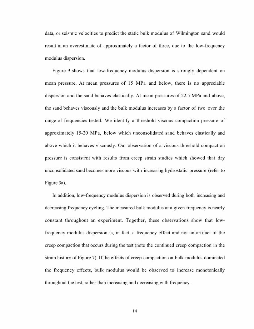
Figure 9 shows that low-frequency modulus dispersion is strongly dependent on

mean pressure. At mean pressures of 15 MPa and below, there is no appreciable

dispersion and the sand behaves elastically. At mean pressures of 22.5 MPa and above,

the sand behaves viscously and the bulk modulus increases by a factor of two over the

range of frequencies tested. We identify a threshold viscous compaction pressure of

approximately 15-20 MPa, below which unconsolidated sand behaves elastically and

above which it behaves viscously. Our observation of a viscous threshold compaction

pressure is consistent with results from creep strain studies which showed that dry

unconsolidated sand becomes more viscous with increasing hydrostatic pressure (refer to

Figure 3a).

In addition, low-frequency modulus dispersion is observed during both increasing and

decreasing frequency cycling. The measured bulk modulus at a given frequency is nearly

constant throughout an experiment. Together, these observations show that low-

frequency modulus dispersion is, in fact, a frequency effect and not an artifact of the

creep compaction that occurs during the test (note the continued creep compaction in the

strain history of Figure 7). If the effects of creep compaction on bulk modulus dominated

the frequency effects, bulk modulus would be observed to increase monotonically

throughout the test, rather than increasing and decreasing with frequency.

15

We also examined the effects of pressure amplitude on low-frequency modulus

dispersion. The experimental procedure is identical to that described previously in this

section, except that the mean pressure is held constant at 27.5 MPa and the oscillation

pressure amplitude is varied between 2 and 10 MPa. These results can be found in

Appendix C.

Attenuation Measurements

To measure the quasi-static attenuation as a function of frequency, we conducted con-

stant frequency tests between 3x10-5 and 3x10-3 Hz. Each test consisted of ten sawtooth

wave cycles at constant frequency. Figure 10 shows an example of the experimental

procedure. Tests were conducted at a mean pressure of 27.5 MPa and a pressure

amplitude of 5 MPa, which corresponds to a strain amplitude of ~2x10-3. The quasi-static

attenuation (1/Q) was calculated by directly measuring the loss in each stress-strain loop,

given by the area in the loop (see inset of Figure 10 for an example stress-strain loop), and

dividing by the maximum energy achieved in each cycle (Tutuncu et al., 1998; Lakes,

1999). The mean of the results from all ten cycles was taken to be the attenuation at each

frequency.

The quasi-static attenuation data derived from the constant frequency tests on dry

Wilmington sand are shown in Figure 11. The error bars represent two standard

deviations away from the mean. Interestingly, the attenuation is nearly constant over the

range of frequencies tested. The attenuation is approximately 0.2, which is quite large

(Q≈5), but is the same order of magnitude as the attenuation measured in Berea sandstone

(this study) and a variety of cemented sandstones at the same strain amplitude over a

16

similar range of frequencies (Tutuncu et al., 1998). For reference, we also measured the

attenuation of 6061 aluminum at a frequency of 4x10-3 Hz. The value obtained,

approximately 0.02, represents the lower limit of the attenuation we can resolve with our

system, since the actual attenuation is orders of magnitude smaller (Brodt et al., 1995).

On the other hand, the attenuation measured in the Wilmington sand samples is an order

of magnitude larger than that measured in the aluminum, and is therefore easily resolved.

Strain-rate effects

To investigate the effects of strain-rate on the strain hardening behavior of

unconsolidated reservoir sands, we conducted triaxial tests under axial strain feedback

control at confining pressures of 15 and 50 MPa, and axial strain-rates varying between

10-7/s and 10-5/s. The samples were deformed at constant strain-rate to an axial strain of

7%, at which point the strain was held constant, and a stress relaxation test was

performed. The results are shown in Figure 12. All of the samples were preloaded to a

hydrostatic stress equal to twice the testing confining pressure (samples tested at a

confining pressure of 50 MPa were preloaded to 100 MPa), and allowed to creep for 6

hours prior to the start of the test. No evidence of brittle failure was observed in any of

the samples.

The stress-strain curves in Figure 12 qualitatively reproduce the behavior predicted

by viscoelasticity theory. A positive relationship between strain-rate and differential

stress is observed at both 15 and 50 MPa. For example, at 7% axial strain, the amount of

differential stress stored in the sample increases from 50 MPa, at a strain-rate of 10-7/s, to

58 MPa, at a strain-rate of 10-5/s. While this difference can be considered small, it is sig-

17

nificant, and greater than the variation due to sample heterogeneity. Related to the rate-

controlled strain hardening is the positive relationship between the initial Young’s

modulus and strain-rate. Notice how the stiffness at the start of the test is strongly

dependent on the strain-rate.

Stress relaxation tests were performed following the triaxial tests to test whether or

not the constitutive behavior of the samples changed during deformation. For example, the

samples might be expected to behave more elastically during deformation as porosity is

reduced and the number of contact points between grains is increased. However, our

results show that unconsolidated sands still behave viscously, even after being deformed

to 7% axial strain. As expected, the samples that were deformed the fastest exhibit the

largest stress relaxation, because deforming the samples at higher strain-rates allows more

stress to be stored, and less creep to occur during loading.

DISCUSSION

It is important to understand the effect that a viscous component of deformation has

on the mechanical behavior of a material. How large is the viscous contribution to the

overall deformation? Over what range of time will creep strain occur? Will creep strain

occur indefinitely for a given stress state? Is it possible to predict the amount of creep

strain in a reservoir prior to drilling? This information is necessary for the accurate

prediction of porosity loss in unconsolidated sand reservoirs with depletion, for example.

For dry unconsolidated sand, the creep strain is slightly larger than the magnitude of

the instantaneous strain at moderate hydrostatic pressures (15 to 30 MPa). The majority

of the creep strain occurs within hours to days. While creep strain has been observed to

18

follow a power-law function of time, it is unknown as to whether this power-law

function can be extrapolated outside the maximum observation time of 5 days. This is im-

portant considering that the time-scale most appropriate to reservoirs is on the order of

tens of years and not tens of hours. Understanding how creep strain changes with loading

rate is important, but it is probably sufficient to simply load samples as rapidly as

possible if an accurate description of creep strain is all that is needed.

Creep strain manifests itself during initial loading, but not during unloading or

reloading. Interestingly, we also observe a threshold viscous compaction pressure during

frequency cycling tests which marks the transition between elastic and viscous behavior.

For Wilmington sand the threshold pressure is approximately 15-20 MPa. For reference,

the maximum in situ effective pressure the samples have seen is between 15 and 20 MPa.

It appears that viscous behavior only occurs when the sample is loaded beyond the

maximum stress it experienced in the field. This implies that unconsolidated sand might be

well described by an elastic-viscoplastic phenomenological model and that the onset of

creep strain could be used as an indication that the maximum in situ stress had been

exceeded.

Frequency cycling tests revealed that creep strain is observable in the frequency

domain as bulk modulus dispersion. It is important to note that the range of frequencies

tested, 10-5 to 10-2 Hz, is several orders of magnitude below the frequency range of

seismic surveys and well-logging sonic tools. In addition, as the strain amplitude is

decreased toward seismic strains, the modulus approaches the low-frequency limit and

not the high-frequency limit as might be expected. Interpreting the bulk modulus

19

measured at seismic frequencies to be the static modulus for the reservoir would result in

an overestimation of approximately a factor of three.

We have concentrated our study on dry samples in order to eliminate poroelastic

effects. Poroelastic effects such as squirt or local-flow modulus dispersion generally occur

in the kHz to MHz range, depending on the viscosity of the saturating fluid and the pore

space geometry of the saturated material (Mavko and Jizba, 1991). Because Wilmington

sand is well drained (30% porosity, permeability on the order a Darcy), we expect that

the behavior of dry samples and saturated samples should be similar at low-frequencies

(<1 Hz).

CONCLUSIONS

Dry unconsolidated sand has been observed to exhibit creep strain under a variety of

constant stress conditions. The creep strain has been observed to follow a power law

function of time, but a linear function of pressure. Creep strain is facilitated by the

presence of ductile minerals, which suggests that the physical mechanism for creep strain

is grain rearrangement. Creep strain represents a significant portion of the total strain, and

is of the same order of magnitude as the instantaneous strain at pressures great than 15

MPa. The instantaneous strain is a non-linear function of confining pressure, and can be

empirically described using a power law. We interpret creep strain to represent a viscous

component of deformation, and predict frequency- and rate-dependent behavior by

placing our observations in the context of linear viscoelasticity theory.

Interestingly, frequency cycling tests reveal that viscous behavior occurs only above a

threshold viscous compaction pressure, which was found to be approximately 15 MPa.

20

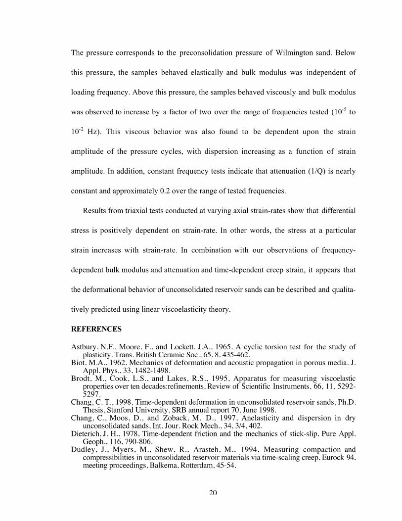
The pressure corresponds to the preconsolidation pressure of Wilmington sand. Below

this pressure, the samples behaved elastically and bulk modulus was independent of

loading frequency. Above this pressure, the samples behaved viscously and bulk modulus

was observed to increase by a factor of two over the range of frequencies tested (10-5 to

10-2 Hz). This viscous behavior was also found to be dependent upon the strain

amplitude of the pressure cycles, with dispersion increasing as a function of strain

amplitude. In addition, constant frequency tests indicate that attenuation (1/Q) is nearly

constant and approximately 0.2 over the range of tested frequencies.

Results from triaxial tests conducted at varying axial strain-rates show that differential

stress is positively dependent on strain-rate. In other words, the stress at a particular

strain increases with strain-rate. In combination with our observations of frequency-

dependent bulk modulus and attenuation and time-dependent creep strain, it appears that

the deformational behavior of unconsolidated reservoir sands can be described and qualita-

tively predicted using linear viscoelasticity theory.

REFERENCES

Astbury, N.F., Moore, F., and Lockett, J.A., 1965, A cyclic torsion test for the study ofplasticity, Trans. British Ceramic Soc., 65, 8, 435-462.

Biot, M.A., 1962, Mechanics of deformation and acoustic propagation in porous media. J.Appl. Phys., 33, 1482-1498.

Brodt, M., Cook, L.S., and Lakes, R.S., 1995, Apparatus for measuring viscoelasticproperties over ten decades:refinements, Review of Scientific Instruments, 66, 11, 5292-5297.

Chang, C. T., 1998, Time-dependent deformation in unconsolidated reservoir sands, Ph.D.Thesis, Stanford University, SRB annual report 70, June 1998.

Chang, C., Moos, D., and Zoback, M. D., 1997, Anelasticity and dispersion in dryunconsolidated sands, Int. Jour. Rock Mech., 34, 3/4, 402.

Dieterich, J. H., 1978, Time-dependent friction and the mechanics of stick-slip, Pure Appl.Geoph., 116, 790-806.

Dudley, J., Myers, M., Shew, R., Arasteh, M., 1994, Measuring compaction andcompressibilities in unconsolidated reservoir materials via time-scaling creep, Eurock 94,meeting proceedings, Balkema, Rotterdam, 45-54.

21

Dvorkin, J. and Nur, A., 1993, Dynamic poroelasticity: A unified model with the squirt andthe Biot mechanism, Geophys., 58, 524-533.

Finkbeiner, T,. Zoback, M., Flemings, P., and Stump, B., 2000, Stress, pore pressure, anddynamically constrained hydrocarbon columns in the South Eugene Island 330 Field,northern Gulf of Mexico, AAPG Bulletin, 85, 6, 1007-1031.

Griffiths, D.V., 1994, Coupled Analysis in Geomechanics, in Viscoplastic Behavior ofGeomaterials, Cristecu, N.D. and Gioda, G., eds., Spinger-Verlag, New York, 245-318.

Hagin, P., and Zoback, M.D., 2002b, Viscous deformation of unconsolidated reservoirsands (Part 2): Linear viscoelastic models, in press.

Kosloff, D. and Scott, R.F., 1980a, Finite Element Simulation of Wilmington Oil FieldSubsidence: I, Linear modelling, Tectonophysics, 65, 339-68.

Kosloff, D. and Scott, R.F., 1980b, Finite Element Simulation of Wilmington Oil FieldSubsidence: II, Nonlinear modelling, Tectonophysics, 70, 159-83.

Kronenberg, A.K., Kirby, S.H., and Pinkston, J., 1990, Basal slip and mechanicalanisotropy of biotite, J. Geophysical Research, 95, B12, 19,257-19,278.

Lakes, R.S. 1999, Viscoelastic Solids, CRC Press LLC, Boca Raton, Florida.Lerouiel, S., Kabbaj, M., Tavenas, F., and Bouchard, R., 1985, Stress-strain-strain rate

relation for the compressibility of sensitive natural clays, Geotechnique, 35, 2, 159-180.Mavko, G., and Jizba, D., 1991, Estimating grain-scale fluid effects on velocity dispersion in

rocks. Geophys., 56, 1940-1949.Mitchell, J.K., Campanella, R.G., and Singh, A., 1968, Soil creep as a rate process, J. Soil

Mech., 94, SM1, 231-256.Moos, D., and Walker, S., 1997, Hydrocarbon detection behind casing in the Wilmington

Field, CA, AAPG Bulletin, 81, 4, 690.Ostermeier, R. M., 1995, Deepwater Gulf of Mexico turbidites-compaction effects on

porosity andpermeability, SPE Formation Evaluation, 79-85.

Prokpovich, N.P., 1983, Tectonic framework and detection of aquifers susceptible tosubsidence, Proc. 1982 Forum on subsidence due to fluid withdrawals, 33-44.

Schenk, L. and Puig, F., 1983, Aspects of compaction/subsidence in the bolivar coast heavyoil fields, higlighted by performance data from the M-6 project areas, Proc. 1982 Forumon subsidence due to fluid withdrawals, 109-120.

Tutuncu, A.N., and Sharma, M.M., 1992, The influence of grain contact stiffness and framemoduli in sedimentary rocks. Geophys. 57, 1571-1582.

Tutuncu, A.N., Podio, A.L., Gregory, A.R., and Sharma, M.M., 1998, Nonlinear viscoelasticbehavior of sedimentary rocks, Part I: Effect of frequency and strain amplitude.Geophys., 63, 184-194.

Wood, D.M., 1990. Soil Behaviour and Critical State Soil Mechanics, CambridgeUniversity Press, New York.

Worall, W.E., 1968, Clays: Their nature, origin, and general properties, Maclaren and Sons,London.

Yale, D.P, Nabor, G.W., Russel, J.A., Pham, H.D., and Yous, M., 1993, Application ofvariable formation compressibility for improved reservoir analysis: SPE-26647, in SPEAnnual Technical Conference Proceedings: Society of Petroleum Engineers.

APPENDIX A: SAMPLE DESCRIPTION

Samples of unconsolidated sand were obtained from oil reservoirs in South Eugene

Island field in the Gulf of Mexico (Lentic sand) and the Wilmington Field in Long Beach,

22

California (Wilmington sand). Additional samples were synthetically constructed in the

lab by volumetrically mixing disaggregated Ottawa sand with wetted Na-montmorillonite

clay in amounts varying between 0 and 15% to a nominal initial porosity of 30%.

The Wilmington sand samples were obtained from cores of the Upper Terminal zone

of the Wilmington turbidite sequence, taken from a depth of approximately one kilometer.

Wilmington sand is primarily composed of 30% quartz, 20% feldspars, 20% biotite mica,

20% metamorphic rock fragments, and 10% smectite clays. It has a mean grain size of 300

mm. Initial porosity is approximately 35% for all of the samples tested. The samples

contain residual hydrocarbons and soft tars, which serve to provide some cohesion

between the otherwise friable grains.

The Lentic sand samples were obtained from the South Eugene Island field core SEI-

316/A-12, taken at a depth of approximately 2.5 kilometers. Lentic sand is composed of

65% quartz, 10% feldspars, 20% volcanic rock fragments, and trace amounts of clay. The

mean grain size is approximately 70 mm. The initial porostiy is approximately 35%, and

the permeability is several Darcies.

Samples of both the Lentic and Wilmington sands were obtained from four-inch di-

ameter core sections that were kept sealed and refridgerated in an attempt to preserve the

in situ chemical and mechanical states. One-inch diameter core plugs were plunge cut with

a stainless steel core barrel, then extruded into polyolefin jacketing material and trimmed

to a nominal length of two inches. In an effort to eliminate pore fluid effects, the jacketed

samples were washed with mineral spirits and acetone until the effluent ran clear and then

dried under vacuum at room temperature until the mass was constant (~24 hours). The

23

samples were then wired to one-inch diameter coreholders, inserted into a New England

Research Autolab 2000 standard triaxial testing machine, and connected to a pore line,

which allowed for communication between the pore space and the atmosphere. All

samples were tested room-dry and drained to the atmosphere at room conditions. All of

the tests were repeated at least twice.

The NER Autolab 2000 is a fully servo-controlled conventional triaxial (biaxial)

testing machine, capable of a variety of loading paths (hydrostatic, conventional triaxial,

uniaxial strain, constant mean stress, etc.), with the ability to simultaneously measure

deformation and ultrasonic velocities (P and cross-polarized S) or permeability (10

nanoDarcies to Darcies). The pressure vessel is lowered onto the base plate by sliding

over the axial piston, and secured in place by moving a yoke between the top plate of the

loading frame and the top of the pressure vessel. The axial piston also divides the

pressure vessel into two chambers; the lower one for the application of confining

pressure, and the upper one for the application of axial pressure. When the pressure in

the top chamber exceeds that in the lower chamber, a differential stress is exerted on the

sample. Because the pressures in the lower and upper chambers are coupled through the

piston, only the differential stress and confining pressure can be specified, and the

maximum differential stress increases with decreasing confining pressure. The differential

stress, confining pressure, and pore pressure are generated with three servo-controlled

hydraulic intensifiers. The maximum axial force that can be exerted on a one-inch diameter

sample is 600 kN, the maximum confining pressure is 200 MPa, and the maximum pore

24

pressure is 100 MPa. The accuracy of the pressure transducers is +/- 0.25% of the

maximum pressure value.

Five electronics feedthroughs in the baseplate and one feedthrough in the axial piston

allow for all relevant measurements to be made inside the pressure vessel in close

proximity to the sample. Axial force is measured by a load cell attached to axial piston,

calibrated to 600 kN, with an accuracy of +/- 0.05%. Seal friction between the axial piston

and the top plate of the load frame has been measured to be 3 kN. Axial displacement is

measured by attaching 2 Linear Potentiometers to the sample coreholders. The LCPs

operate on 15 V DC, with half an inch of travel, and an accuracy that is limited by the

National Instruments 12-bit A/D converters to four thousandths of an inch before being

acquired by a Unix-based computer running NER’s Autolab acquisition/control software.

Radial deformation is measured using an LVDT with a quarter-inch of travel and an

accuracy of a hundredth of an inch. The radial LVDT is attached to the sample using a

custom-built chain-gauge. Control signals can be sent from either the computer or the

electronics rack to any of the three hydraulic intensifiers, which in turn operate under

either pressure or displacement control.

25

APPENDIX B: SUMMARY OF EXPERIMENTAL RESULTS

Table 1: Creep Strain Measurements

SampleType

# of tests Pc (MPa) LoadingRate

ev after 6hours

Timeconstant

Comments

Wilmington 5 2 1 MPa/hr 0.002 0.68Wilmington 5 5 1 MPa/hr 0.002 0.65Wilmington 4 10 1 MPa/hr 0.003 0.63Wilmington 4 15 1 MPa/hr 0.002 0.51Wilmington 4 20 1 MPa/hr 0.002 0.51Wilmington 4 25 1 MPa/hr 0.003 0.59Wilmington 4 30 1 MPa/hr 0.003 0.61Wilmington 4 50 1 MPa/hr 0.003 0.53

Lentic 2 30 1 MPa/hr 0.002 0.55Ottawa 2 30 1 MPa/hr 0.0003 0.55

Ottawa/ 5%clay

2 30 1 MPa/hr 0.0007 0.48 Montmorilloniteclay

Ottawa/10% clay

2 30 1 MPa/hr 0.001 0.45 Montmorilloniteclay

Wilmington 2 10 1 MPa/s 0.005 0.1 Note increasedloading rate

Wilmington 2 20 1 MPa/s 0.01 0.1Wilmington 2 30 1 MPa/s 0.015 0.1

Notes on Table 1:

1. Pc refers to confining, or hydrostatic, pressure.

2. Loading Rate is given as pressure/time. Note that the majority of these tests are not

true creep strain tests in the sense that they were conducted in a manner similar to

that shown in Figure 2. The last three tests listed in the table are true creep tests, as

shown in Figure 4

3. ev is the mean volumetric strain measured during the creep tests.

26

4. “Time constant” refers to the exponent that would provide the best fit to the data if it

were modeled as a power law function of time.

5. All of these tests were conducted at room temperature, on dry samples which were

drained to the atmosphere.

Table 2: Stress Relaxation Tests

SampleType

# oftests

Pc(MPa)

e11 final e11 rate(1/s)

sD

(MPa)Time

Constant

Wilmington 2 15 7% 10-5 19 -0.04Wilmington 2 15 7% 10-6 16 -0.05Wilmington 2 15 7% 10-7 13 -0.05Wilmington 2 50 7% 10-5 58 -0.04Wilmington 2 50 7% 10-6 50 -0.04Wilmington 2 50 7% 10-7 50 -0.05

Notes on Table 2:

1. These were triaxial tests, controlled by axial strain (e11) rate until an axial strain of 7%

was reached, at which point the strain was held constant and stress relaxation was

observed for 6 hours.

2. sD refers to the differential stress stored in the sample when the stress relaxation test

began.

3. As in Table 1 above, the time constant refers to the exponent that would best-fit the

data if it were modeled using a power law function of time.

Table 3: Strain-rate Effects in Triaxial Tests

SampleType

# of tests Pc (MPa) e11 final e11 rate

(1/s)

sD (MPa) Apparent

E (MPa)

Wilmington 2 15 7% 10-5 19 1250

Wilmington 2 15 7% 10-6 16 783

Wilmington 2 15 7% 10-7 13 583

27

Wilmington 2 50 7% 10-5 58 2500

Wilmington 2 50 7% 10-6 50 1805

Wilmington 2 50 7% 10-7 50 972

Notes on Table 3:

1. These were triaxial tests run at 2 different confining pressures and 3 different axial

strain rates. The data is shown in Figure 12.

2. sD refers to the differential stress at 7% axial strain.

3. The apparent Young’s modulus (“Apparent E”) measured at the start of the test.

APPENDIX C: STRAIN-AMPLITUDE EFFECTS

To investigate the effects of varying strain-amplitude on the mechanical behavior of

dry Wilmington sand, we conducted frequency cycling tests at constant mean pressure as

a function of pressure amplitude, using pressure amplitude as a proxy for strain ampli-

tude. Figure 7 shows an example of the experimental procedure. Samples are first loaded

to the maximum hydrostatic pressure for the particular test and allowed to creep for 6

hours. A series of sawtooth pressure cycles is then conducted at frequencies between

3x10-5 and 3x10-2 Hz. Frequency is first increased from the low-frequency to the high-

frequency limit, then decreased, and the static bulk modulus is measured during the re-

loading leg of each cycle. We conducted tests at a mean pressure of 27.5 MPa and

pressure amplitudes of 10, 5, and 2 MPa. The results from the frequency cycling tests

investigating the influence of strain amplitude are shown in Figure B-1.

Figure B-1 shows that dispersion increases with pressure (and strain)

amplitude, ranging from a 50% increase in bulk modulus at a pressure amplitude of

28

2 MPa (strain amplitude of order 10-3) to an increase of 100% in modulus at a

pressure amplitude of 10 MPa (strain amplitude of order 10-2). In other words, at

a given frequency, the apparent stiffness increases with strain amplitude. It is also

interesting that the sample behaves more viscously at large pressure amplitudes

and more elastically at small pressure amplitudes. This observation is consistent

with a micromechanical model in which the clay fraction is load bearing (Chang et

al., 1997).

29

Figure 1: Creep strain is dependent upon the presence of hydrous clay minerals. In thesynthetic samples, the amount of creep can be seen to increase with clay content. Thehydrous clay content of the Wilmington sand samples is approximately 15%.Modified from Chang et al., 1997.

0

0.0005

0.001

0.0015

0.002

0.0025

0 5000 1 104 1.5 104 2 104 2.5 104 3 104

Volum

etric

Stra

in (m

m3 /m

m3 )

Time (s)

GOM - Lentic

Wilmington - Upper TerminalWilmington -Upper Terminal

Ottawa Sand - 10% Montmorillonite

Ottawa Sand - 5% Montmorillonite

Ottawa Sand

30

Figure 2: Dry hydrostatic pressure tests show that both instantaneous and viscousdeformation (creep strain) occur simultaneously. Note that the creep strain isnonlinear with time and approximately the same magnitude as the instantaneousstrain.

05

1015

2025

30

00.

005

0.01

0.01

50.

020.

025

0.03

0.03

50.

04

0 10 20 30 40

Conf

inin

g Pr

essu

re (M

Pa)

Volumetric Strain (m

m3/m

m3)

Time (hr)

Confining Pressure

Volumetric Strain

InstantaneousStrain

Creep Strain

31

Figure 3: a) Incremental instantaneous and creep strains corresponding to 5 MPaincremental increases in pressure. The data plotted at each pressure reflect theincreases in strain that occurred during each increase in pressure. Note that above 15MPa the incremental creep strain is the same magnitude as the incrementalinstantaneous strain. b) The cumulative instantaneous volumetric strain is a non-linear function of pressure and can be described empirically using a power law. Referto Figure 2 for an example of the test procedure.

00.

002

0.00

40.

006

0.00

80.

015 10 15 20 25 30 35

Volum

etric

Stra

in (m

m3 /m

m3 )

for 5

MPa

incr

easin

g pr

essu

re in

crem

ents

Confining Pressure (MPa)

Instantaneous Strain

Creep Strain

3a

00.

010.

020.

030.

040.

050.

060 5 10 15 20 25 30 35

Volum

etric

Stra

in (in

/in)

Confining Pressure (MPa)

3b

32

Figure 4: Results from a hydrostatic creep test on Wilmington sand conducted for 5days. Following the creep test the sample was unloaded and partially reloaded in aneffort to qualify whether creep is elastic or plastic deformation. The instantaneousstrain response during unloading and the lack of creep strain during reloadingsuggest that a large part of the total sample deformation (~4% volumetric strain) isirrecoverable.

0

5

10

15

20

25

30

35

40

0

0.01

0.02

0.03

0.04

0.05

0.06

0 50 100 150 200 250 300

Pressure (MPa) strain

Conf

inin

g Pr

essu

re (M

Pa)

Volumetric Strain (m

m3/m

m3)

Time (Hr)

Unload to initial pressure

Creep StrainElastic Recovery

No Creep Strain

Partial Reload

5 days

33

Figure 5: Log-log plot of the creep strain data from Figure 4 reveals that it follows apower law function of time. The data can be described by a power law Atp, where A=15 and p = 0.1. This observation suggests that creep deformation may continue forlong periods of time at decreasing strain rate.

11

1.1

0.01 0.1 1 10 100 1000

Log

volum

etric

stra

in

Log Normalized Time

e(t)=15t0.1

34

Figure 6: Time-dependent deformation in a viscoelastic material is most commonlyobserved as creep strain (a) or stress relaxation (b). Linear viscoelasticity theorypredicts frequency- and rate-dependence for materials that exhibit time-dependence.Specifically, elastic modulus and attenuation should vary with loading frequency (c),and stiffness should increase with strain rate (d). Refer to the text for furtherdiscussion.

35

Figure 7: An example of the test procedure used to measure bulk modulus as a functionof frequency. Samples are loaded at a rate of 5MPa/hr to a confining pressure equalto the mean pressure plus half of the pressure amplitude and allowed to creep for 6hours. A series of load cycles is then conducted at varying frequencies.

05

1015

20

00.

005

0.01

0.01

50.

02

0 10 20 30 40 50 60

Conf

inin

g Pr

essu

re (M

Pa)

Volumetric Strain (m

m3/m

m3)

Time(hr)

Volumetric Strain

Confining PressurePressure Amplitude

MeanPressure

36

Figure 8: Normalized bulk modulus of dry Wilmington sand as a function of frequencyspanning 10 decades. Starting with the low frequency (<1 Hz) pressure-cycling data,notice that bulk modulus increases by a factor of 3 with increasing frequency. Thedata shown comes from a test run at 22.5 MPa hydrostatic pressure with a 5 MPapressure oscillation. Notice that this “low-frequency modulus dispersion” occurs atfrequencies less than those used in seismic data acquisition, and that the bulkmodulus falls below the static modulus predicted using Gassmann theory. The bulkmodulus increases to the Gassmann static limit at approximately 0.1 Hz and thenstays constant as frequency is increased through 1 MHz. While our experiments wereconducted on dry samples, we have included the effects of poroelasticity in thisdiagram by including the predicted behavior of oil-saturated samples according to theBiot-Squirt local-flow theory (Mavko et al., 1998).

0

0.2

0.4

0.6

0.8

1

1.2

1.4

1.00E-05 1.00E-03 1.00E-01 1.00E+01 1.00E+03 1.00E+05 1.00E+07

Frequency (Hz)

Norm

aliz

ed B

ulk

Mod

ulus

Well-log data Ultrasonic data

Pressure-cycling data

Gassmann static limit

Biot-Squirt theory(oil saturation)

Low-frequency dispersion

Seismic data

Static "Modulus"

37

Figure 9: Normalized bulk modulus is plotted as a function of frequency and meanpressure. The arrows indicate the loading procedure used for all of the tests; loadingfrequency is first increased and then decreased. It can be seen that there is a transitionin material behavior around a mean pressure of 15-20 MPa. At lower mean pressures,the bulk modulus is independent of frequency and the material appears to behaveelastically. At higher mean pressures, the bulk modulus can be seen to increase by afactor of two with frequency and the material behaves viscously.

0.5

11.

52

2.5

310

-5

0.00

01

0.00

1

0.01 0.

1

Increasing FrequencyDecreasing Frequency

Norm

alize

d Bu

lk M

odul

us(K

/ K o )

Loading Frequency (Hz)

Pc=7.5MPa

Pc=22.5MPa

Pc=27.5MPa

Pc=15MPa

38

Figure 10: An example of the test procedure used to measure attenuation as a function offrequency. Samples are loaded at a rate of 6 MPa/hr to a confining pressure equal tothe mean pressure plus half of the pressure amplitude and allowed to creep for 6hours. A series of ten loading cycles is then conducted at constant frequency, withfrequency varying between 3x10-5 and 3x10-2 Hz. The attenuation in each cycle iscalculated by directly measuring the loss from the stress-strain curves and dividing itby the maximum energy for that cycle (see inset figure for an example of a stress-strain curve).

05

1015

2025

3035

-0.0

10

0.01

0.02

0.03

0.04

0.05

0.06

0.07

0 20 40 60 80 100

120

Conf

inin

g Pr

essu

re (M

Pa)

Volumetric Strain (m

m3/m

m3)

Time (Hr)

Confining Pressure

Volumetric Strain

25

26

27

28

29

30

31

0.0925 0.0926 0.0927 0.0928

A typical stress-strain hysteresis loop

Pc(M

Pa)

Volume Strain

Pc (M

Pa)

Volumetric Strain

39

Figure 11: Attenuation as a function of frequency in dry Wilmington sand. Attenuationis nearly constant over the range of frequencies tested and is approximately 0.2(Q≈5).

0.01

0.1

1

10-5 0.0001 0.001 0.01

Atte

nuat

ion

(1/Q

)

Frequency (Hz)

Dry Berea Sanstone

6061 Aluminum

Dry Wilmington Sand

40

Figure 12: Results from triaxial tests performed on dry Wilmington sand. The sampleswere preconsolidated under a hydrostatic stress equal to twice the testing confiningpressure and allowed to creep for 6 hours prior to the triaxial stage of the test. Notethat the differential stress at a given strain increases with strain rate, as predicted bylinear viscoelasticity theory.

41

Figure B-1: Normalized bulk modulus is plotted as a function of frequency andoscillation pressure amplitude at a mean pressure of 27.5 MPa. Observe that as theoscillation pressure amplitude increases from 2 MPa to 10 MPa, the degree ofmodulus dispersion increases from a factor of 1.4 to a factor of 2. In other words, thematerial behaves more viscously with increasing oscillation pressure amplitude.

0.5

11.

52

2.5

310

-5

0.00

01

0.00

1

0.01 0.

1

Increasing FrequencyDecreasing Frequency

Norm

alize

d Bu

lk M

odul

us

(K /

K o )

Loading frequency (Hz)

delPc=10MPa

delPc=2MPa

42

CHAPTER 2

VISCOUS DEFORMATION OF UNCONSOLIDATED RESERVOIR SANDS

(PART II): LINEAR VISCOELASTIC MODELS

This paper was written with Mark Zoback and has been accepted by Geophysics

ABSTRACT

Laboratory creep experiments show that dry unconsolidated reservoir sands follow a

power law function of time (at constant stress) and cyclic loading tests (at quasi-static

frequencies of 10-6 to 10-2 Hz) show that the bulk modulus increases by a factor of two

with increasing frequency while attenuation remains constant. In this paper we attempt to

model these observations using linear viscoelasticity theory by considering several simple

phenomenological models. We investigated two classes of models; spring-dashpot

models, which are represented by exponential functions with a single relaxation time, and

power law models. Although almost all of the models considered were capable of fitting

the creep data with time, they result in very different predictions of attenuation and bulk

modulus dispersion. We used the model parameters derived from fitting the creep strain

to predict the bulk modulus dispersion and attenuation as a function of frequency, to find

a single phenomenological model (and model parameters) that could explain the

material’s creep response with time as well as its dispersion and attenuation

characteristics. Spring-dashpot models, such as the Burgers and standard linear solid

models, produce reasonable fits to the creep strain and bulk modulus dispersion data, but

43

do not reproduce the attenuation data. We find that a combined power law-Maxwell creep

model adequately fits all of the data. Extrapolating the power law-Maxwell creep model

out to 30 years (to simulate the lifetime of a reservoir) predicts that the static bulk

modulus is only 25% of the dynamic modulus. Including the instantaneous component of

deformation into the previous prediction results in 2% total vertical strain at the wellbore,

in good agreement with field observations.

INTRODUCTION

Laboratory studies of the mechanics of unconsolidated sands and clays have shown

that there is a time-dependent component of deformation (Wood, 1990; Chang et al.,

1997; Dudley, 1994; Ostermeier, 1995). While time-dependent deformation is typically

associated with pore-fluid effects and poroelasticity (Biot, 1962; Griffiths, 1994; Mavko

and Jizba, 1991), recent laboratory studies of unconsolidated reservoir sands have shown

that time-dependent deformation may also be attributed to the viscous behavior of clays

in the dry frame and associated grain rearrangement (ex. Chang et al., 1997).

Recent studies of time-dependent creep strain under constant stress conditions in both

saturated and unsaturated unconsolidated sands suggest that their behavior can be

described using linear viscoelastic phenomenological models. Ostermeier (1995)

characterized observations of creep strain under hydrostatic loading conditions in

saturated Gulf of Mexico reservoir sands using a Standard Linear Solid viscoelastic

model. Chang et al. (1997) found that a Standard Linear Solid model also described the

creep strain behavior of room dry unconsolidated sands from the Wilmington Field,

California, under a variety of loading conditions. Dudley et al. (1994) observed creep

44

strain in saturated Gulf of Mexico reservoir sands under uniaxial strain conditions and

found that their data could be described by a power law function of time. De Waal and

Smits (1988) found that a power law function could describe the stress rate-dependent

uniaxial compaction of a wide variety of reservoir sands and sandstones.

In this paper we expand upon our experimental data (see Chapter 1) for samples

obtained from the Wilmington field in Long Beach, CA, to distinguish among various

linear viscoelastic models and arrive at a constitutive law that describes the behavior of

unconsolidated reservoir sands. We provide experimental evidence to argue that

Wilmington sand is a linear material and that linear viscoelastic phenomenological

models are therefore appropriate for describing its behavior. We also show that applying

linear viscoelastic models to creep strain data quantitatively predicts the frequency-

dependence of bulk modulus and quasi-static attenuation in unconsolidated sands.

The primary advantage of employing phenomenological models is that the

deformational behavior of a material can be predicted without any knowledge of the

mechanics responsible for the deformation. Constructing a physical model to describe

time-dependent deformation in unconsolidated sands is difficult because such

deformation can result from a variety of mechanical and chemical effects.

Phenomenological models side-step this complexity and provide a means for bridging

laboratory observations of time-dependent deformation in unconsolidated sands with

similar observations made in the field.

45

SUMMARY OF OBSERVATIONS

A detailed explanation of our experiments and results can be found in the companion

paper (Chapter 1). In that paper we describe three types of experiments to explore the

influence of time- and frequency-dependent effects on the mechanical behavior of

unconsolidated reservoir sand: creep strain tests, pressure-cycling tests to measure

modulus as a function of frequency, and pressure-cycling tests to measure attenuation as

a function of frequency.

A typical creep strain experiment on dry Wilmington sand (refer to Figure 4, Chapter

1) begins by loading the sample to some initial hydrostatic pressure to seat the sample

and then quickly increasing the load to the test pressure. In this case, the pressure was

increased from 2 MPa to 30 MPa in one minute. The pressure is then held constant for 5

days. Notice that the creep strain is highly non-linear as a function of time. The majority

of the deformation occurs within the first ten hours, and while the rate of deformation

decreases rapidly, deformation continues to occur throughout the test. Also note that the

amount of creep strain is significant – more than a tenth of a percent of axial strain occurs

over 5 days.

While creep strain is a non-linear function of time, it is a linear function of pressure

(refer to Figure 3a, Chapter 1). The creep component of deformation is equal for each

pressure step, indicating that it is a linear function of pressure. More importantly, the

creep component of deformation exceeds the instantaneous component at confining

pressures above 15 MPa, so the viscous contribution to the overall deformation is

significant and in fact will control the behavior of unconsolidated sand at moderate to

high pressures.

46

We also investigated the frequency dependence of bulk modulus and attenuation as a

function of the effective mean pressure. Our measurements of bulk modulus as a function

of frequency yielded to two important results (refer to Figure 9, Chapter 1). The first is

that bulk modulus is observed to increase by a factor of 2 over the range of loading

frequencies tested (10-5 – 10-2 Hz). The second is that this observed low-frequency

modulus dispersion only occurs above a certain threshold pressure, in this case

approximately 15-20 MPa. Below this threshold pressure, bulk modulus is independent of

frequency, and the sample behaves elastically. Above the threshold pressure, bulk

modulus doubles with increasing frequency, indicating that there is a viscous component

of deformation. In other words, we can identify a threshold viscous compaction pressure,

above which we see the onset of viscous deformation in an otherwise elastic material.

This pressure corresponds to the in situ preconsolidation pressure of Wilmington sand

(P.S. Hara – personal communication). As most offshore fields have been subjected to

monotonically increasing loading history, it may be assumed that they are at maximum in

situ effective stress at the time of discovery, and therefore may be prone to creep from the

start of production.

The same experiments that produced the bulk modulus data also provided information

about the quasi-static attenuation in the sample. Note that the observed attenuation is due

to viscous dry-frame effects and not poroelasticity. Attenuation at quasi-static frequencies

and relatively large strain amplitudes (10-3 axial strain amplitude) can be calculated from

the degree of stress-strain hysteresis during a cycle. Attenuation was observed to be

constant and approximately 0.2 over the range of frequencies tested (10-5-10-2 Hz) at a

mean effective pressure of 27.5 MPa (refer to Figure 11, Chapter 1).

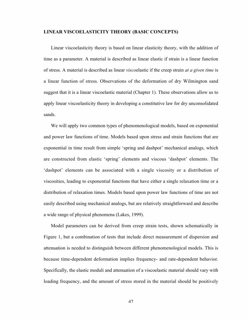
47

LINEAR VISCOELASTICITY THEORY (BASIC CONCEPTS)

Linear viscoelasticity theory is based on linear elasticity theory, with the addition of

time as a parameter. A material is described as linear elastic if strain is a linear function

of stress. A material is described as linear viscoelastic if the creep strain at a given time is

a linear function of stress. Observations of the deformation of dry Wilmington sand

suggest that it is a linear viscoelastic material (Chapter 1). These observations allow us to

apply linear viscoelasticity theory in developing a constitutive law for dry unconsolidated

sands.

We will apply two common types of phenomenological models, based on exponential

and power law functions of time. Models based upon stress and strain functions that are

exponential in time result from simple ‘spring and dashpot’ mechanical analogs, which

are constructed from elastic ‘spring’ elements and viscous ‘dashpot’ elements. The

‘dashpot’ elements can be associated with a single viscosity or a distribution of

viscosities, leading to exponential functions that have either a single relaxation time or a

distribution of relaxation times. Models based upon power law functions of time are not

easily described using mechanical analogs, but are relatively straightforward and describe

a wide range of physical phenomena (Lakes, 1999).

Model parameters can be derived from creep strain tests, shown schematically in

Figure 1, but a combination of tests that include direct measurement of dispersion and

attenuation is needed to distinguish between different phenomenological models. This is

because time-dependent deformation implies frequency- and rate-dependent behavior.

Specifically, the elastic moduli and attenuation of a viscoelastic material should vary with

loading frequency, and the amount of stress stored in the material should be positively

48

correlated with strain rate at a given strain. Therefore, by using an appropriate model and

the parameters derived from creep strain tests, it should be possible to predict the change

of elastic moduli and attenuation as a function of frequency. In Figure 1, note that while

the creep strain responses are qualitatively similar among the various models, the

modulus and attenuation responses are distinct. We will use this observation to identify

the model that best describes the behavior of Wilmington sand in a later section.

LINEAR VISCOELASTICITY THEORY (MATHEMATICAL DETAILS)

In this section we outline the theoretical methods used to model our Wilmington sand

data. For more details on the mathematics, see Lakes (1999), and an exhaustive treatment

of linear viscoelasticity theory can be found in Tschoegl (1989). As mentioned in the

previous section, we are going to find the best-fitting model of the behavior of

Wilmington sand by exploiting the differences in modulus and attenuation between the

various models in the frequency domain. Therefore, we need a procedure that enables the

prediction of stiffness and attenuation in the frequency domain from creep data collected

in the time domain. After describing the general procedure, we follow the procedure

through from beginning to end using the Standard Linear model as an example. The

mathematical details for the other models used in this paper are provided in the

Appendix.

Constitutive equations for linear viscoelastic materials are based upon the Boltzmann

superposition principle, which states that the effect of a compound cause is the sum of the

effects of the individual causes (Lakes, 1999). In other words, if the response to a step

stress or strain function is known, the response to any arbitrary stress or strain function

49

can be constructed by breaking the function into step functions and summing the

response to each step. Figure 2 shows how the stress response to constant strain rate

boundary conditions can be constructed using the stress relaxation response to a step

strain function and Boltzmann superposition. Figure 2a shows a step strain function

occurring at time t1 and the corresponding stress response, in this case, an instantaneous

increase in stress followed by stress relaxation as a function of time. Figure 2b shows a

second step in strain added to the first at time t2 and the corresponding stress response,

which is just the stress response from Figure 2a, added to the existing stress history at t2.

The overall stress response to the 2 step strain functions is just the sum of the individual

stress responses, as shown in Figure 2b. Mathematically, the strain in Figure 2b can be

written as a superposition of the two step functions, where H(t) indicates a step function:

e(t) = eo[H(t-t1) + H(t-t2)], (1)

and the corresponding stress response can be described using Boltzmann superposition,

s(t) = eo[E(t-t1) + E(t-t2)], (2)

where E(t) is the stress relaxation response function. Applying the Boltzmann

superposition principle and integrating with respect to strain (to avoid requiring that the

strain history be a differential function of time) allows the stress response to an arbitrary

strain function to be written as,

(3)

where the integral is evaluated over the time interval 0 to t, and t is the time variable,

such as t1 mentioned in Figure 2. Equation 3 is one variant of the Boltzmann integral.

†

s(t) = E(t-t )de0

t

Ú ,

50

Reversing the role of stress and strain and applying the same arguments as in Equation 3

above results in a complementary relation:

(4)

where J(t) is the creep compliance function.

The stress response to a constant strain rate can be constructed by first assuming that

the rate of strain (the slope in a strain-time plot) can be represented by step functions of

strain spaced at an appropriate time interval, as shown in Figure 2c. A higher strain rate is

achieved by spacing the strain steps more closely in time. By substituting into equation 3

and changing variables, (using x as a dummy variable for the sake of integration),

(5)

and by Liebnitz’ rule (Lakes, 1999; Hildebrand, 1962),

(6)

which means that the slope of the stress response decreases as a function of time, as

shown in Figure 2c. Thus, linear viscoelastic materials exhibit nonlinear stress-strain

curves (because the stress response to a constant strain rate is a nonlinear, concave-

downward function of time) and the stress-strain curve is strain-rate dependent.

Having created a framework for the construction of linear viscoelastic constitutive

equations using the Boltzmann superposition principle, we now develop a means to relate

creep strain functions to stress relaxation functions in both the time and frequency

domains, by making use of the properties of Laplace transforms. We start by relating the

creep function J(t) to the relaxation function E(t) in the time domain. Performing the

†

s(t) = E(t-t ) dedt0

t

Ú dt =dedt

E(t-t )0

t

Ú dt = -dedt

E(x)0

t

Ú dx,

d s(t)

dt=

de

dtE(t),

†

e(t) = J(t- t)d0

t

Ú e,

51

E

Laplace transform of the Boltzmann superposition integrals which contain the J(t) and

E(t) terms (Equations 3 and 4 above) results in the following algebraic expressions as a

funtion of s, where s is the tranform variable:

(7)

(8)

Combining Equations 7 and 8 results in the following relationship between E(s) and J(s),

(9)

which allows E(t) to be derived from J(t) by performing the Laplace transform of J(t) to

J(s), solving for E(s) using Equation 9, and then performing the reverse Laplace

transform on E(s) to find E(t).

Creep and relaxation functions of time can also be converted to functions of

frequency by making use of the Boltzmann superposition integral and Laplace

transforms. Assume that the strain history is sinusoidal, e(t) = eo eiwt, where w is angular

frequency and eiwt is the Euler equation for complex variables. Starting with the

Boltzmann integral, and setting the lower limit of integration to -∞,

(10)

Next, decompose the relaxation function into the sum of a shifted time-dependent term,

, and a constant term, Eeq, which represents the modulus at equilibrium,

(11)

Substituting the sinusoidal strain history into Equation 10 yields,

s(s) = sE(s)e(s)

e(s) = sJ(s)s(s)

E(s)J(s) =1

s2,

†

s(t) = E(t - t) dedt

dt-•

t

Ú .

E(t) = E (t) + Eeq.

52

(12)

Substituting the shifted time variable x (x=t-t) into the above equation reveals that the

stress response to a sinusoidal strain history is also sinusoidal, but no longer in phase:

(13)

Equation 13 can be rewritten using Euler’s equation to produce a stress-strain relation

which depends on the complex modulus, E*(w), as a function of both frequency and time:

(14)

with

(15)

(16)

E’(w) from equation 15 represents the real part of the complex modulus and is referred to

as the storage modulus, while E’’(w) from equation 16 is the imaginary part of the

complex modulus and is known as the loss modulus.

Given the bulk modulus and attenuation tests we performed as a function of

frequency (see Chapter 1), it is necessary to extract the magnitude of the complex

modulus and the loss tangent from the above equations in order to model the data. The

magnitude of the complex modulus is required for comparison with our bulk modulus

data, since the data was obtained through load cycling, and any modulus measured

†

s(t) = Eeqeoeiwt + iweo E (t - t)

-•

t

Ú eiwt dt.

†

s(t) = eoeiwt [Eeq + w E (x)

0

•

Ú sin(wx)dx + iw E (x)0

•

Ú cos(wx)dx].

s(t) = E*(w)e(t) = [ ¢ E (w)+ i ¢ ¢ E (w)]e(t ),

†

E (t) = E(t) - Eeq ,

¢ E (w) ≡ Eeq +w E (x)sin(wx)dx0

•

Ú ,

and

¢ ¢ E (w) ≡ w E (x)cos(wx)dx0

•

Ú .

53

dynamically is inherently complex (Lakes, 1999, Mavko et al., 1998). The loss tangent is

approximately equal to 1/Q and is given by the ratio of the loss and storage moduli:

(17)

In order to derive a constitutive equation for dry Wilmington sand, it is necessary to

convert observations of creep strain in the time domain to stiffness and attenuation as a

function of frequency. We therefore must develop a procedure using Boltzmann

superposition integrals and Laplace transforms to interchange creep strain and stress

relaxation functions and the time and frequency domains. We now work through this for

a Standard Linear Solid to illustrate the general procedure.

Standard Linear Solid Model

We start with the stress relaxation function,

(18)

where E(t) is stiffness as a function of time, E∞ is the stiffness at infinite time, E1 is the

change in stiffness during relaxation, and tr refers to the characteristic relaxation time. In

this equation, stiffness is at a maximum at time equal to zero, and then decays as a

function of time as determined by the characteristic relaxation time in the exponential

function. With regards to the phenomenological elements of the model, each stiffness

corresponds to a spring, and the exponential function corresponds to a dashpot.

To convert the stress relaxation function, E(t), to a creep strain function, J(t), we first

take the Laplace transform of Equation 18 to obtain

1/ Q ª tand(w) ≡¢ ¢ E (w)¢ E (w)

.

E(t) = E• + E1e-t / t r ,

54

(19)

Next, we find J(s) by applying Equation 9, yielding,

(20)

so, after some algebra to reduce the resulting equation, we find,

(21)

The final step is to solve for the creep strain function, J(t), by taking the inverse Laplace

transform of Equation 21. This can be solved by comparison to the forward Laplace

transform shown in Equations 18 and 19, and results in,

(22)

where all of the parameters are the same as those in the stress relaxation equation that we

started with, except for the exponential time constant t c, which now refers to the

characteristic creep time, which is not the same as the characteristic relaxation time, tr.

The creep time and relaxation time can be related using the relation,

(23)

E(s) =E•

s+

E1

s+1t r

Ê

Ë Á Á

ˆ

¯ ˜ ˜

.

J(s) =1

s2E(s),

J(s) =

1

E•

Ê

Ë Á Á

ˆ

¯ ˜ ˜

s-

E1

E•(E1 + E•)

s+E•

(E1 + E•)t r

Ê

Ë Á Á

ˆ

¯ ˜ ˜

.

J(t) =1

E•

-E1

E•(E1 + E•)e-t / t c ,

tc = t r(1+E1

E•

),

55

so the creep time and relaxation time are nearly equal if the change in stiffness during

relaxation is very small in comparison to the stiffness at infinite time.

The next step of the procedure is to derive equations for attenuation and complex

stiffness as a function of frequency, using Laplace transforms and the stress relaxation

equation for a Standard Linear Solid (Equation 18). Recall that our motivation is to

predict the frequency dependence of stiffness and attenuation of unconsolidated sand

using time-dependent creep strain data. We begin by combining the stress relaxation

equation (Equation 18) with Equations 15 and 16 to find the storage modulus, E’(w), and

loss modulus, E”(w), as functions of frequency:

(24)

(25)

To make comparisons with our bulk modulus dispersion and attenuation data, we need to

calculate the magnitude of the complex modulus and the loss tangent from the loss and

storage moduli. As shown in Equation 17, the loss tangent, which approximates 1/Q, is

given by the ratio between the loss and storage moduli, so combining Equations 24 and

25 yields:

(26)

where t is related to the characteristic relaxation time in the following way:

(27)

¢ E (w) = E• + E1

w2t r2

1+w2t r2

,

¢ ¢ E (w) = E1

wtr

1+w2t r2.

1/ Q ª tand(w) =(E1 E•)

1+ E1 E•

wt

1+w2t2,

t = t r 1+ E1 E• .

56

The magnitude of the complex modulus is defined as,

(28)

and for the case of the Standard Linear Solid, after combining Equations 24 and 25 with

Equation 28,

(29)

In summary, we used linear viscoelasticity theory and Laplace transforms to develop

relations between stiffness relaxation and creep strain in the time domain. We also

derived equations for attenuation and complex modulus in the frequency domain for a

Standard Linear Solid and corresponding equations for the other phenomenological

models shown in Figure 1 are presented in the Appendix. In the following sections, we

find the best-fitting model (and model parameters) for our data.

MODELING CREEP, DISPERSION AND ATTENUATION

In this section we will only consider the time-dependent component of the

deformation, since the instantaneous contribution to the deformation is described in the

companion paper (Chapter 1). We start by finding the various model parameters that

result in the smallest least-squares misfit to the creep strain data, apply the models by

predicting modulus dispersion and attenuation as a function of loading frequency, and

then compare the predicted responses with the dispersion and attenuation data. The model

that has the least overall misfit to the data is selected as the preferred constitutive law for

describing the behavior of dry Wilmington sand.

E*(w) = ( ¢ E + i ¢ ¢ E )( ¢ E - i ¢ ¢ E ) = ¢ E 2 + ¢ ¢ E 2 ,

E*(w) = (E• + E1

w2t2

1+w2t2)2 + (E1

wt

1+w2t2)2.

57

To make a meaningful comparison between the models data were selected from creep

strain and loading-frequency cycling experiments conducted at hydrostatic pressures

between 27.5 and 30 MPa. We consider the data in this pressure range because it is above

the threshold viscous compaction pressure, which ensures that the material exhibits

viscous behavior.

Modeling Creep Strain

The creep strain data and best-fitting results from the various phenomenological

models are shown in Figure 3. The data is best described by combining power law creep

and Maxwell solid models. However, the single-element power law, standard linear solid,

and Burgers models all reproduce the overall trend of the data. The predictions of the

Maxwell and Voight solid models are not shown because they cannot reproduce the data.

The Maxwell solid produces creep strain functions that are linear in time (Figure 1), and

the Voight solid cannot be used to model our creep strain data because it does not exhibit

an instantaneous component of deformation, which was clearly observed in the data.

The general procedure for applying the various models involved obtaining values for

all of the measurable parameters and then solving for the remaining parameters by

minimizing the least-squared misfit to the data. Both the power law and standard linear

solid models are three component models involving 2 stiffness parameters and 1 power or

exponent variable to control the time dependence. Specifically, the power and exponent

each determine the point of maximum curvature of their respective creep strain function

(the maximum value of the second derivative of the creep strain function). The Burgers

solid and the combined power law-Maxwell solid have 4 parameters – 2 stiffness

58

variables and 2 exponents which determine the point of maximum curvature and the long

term steady-state viscous flow rate (Figure 1). Of these parameters, the instantaneous

stiffness could be determined from the data, leaving 2 free parameters in the case of the

standard linear solid and power law models, and 3 free parameters in the case of the

Burgers solid model.

The fact that all three of the functions shown in Figure 3 are capable of reasonably

fitting the general trend of the data makes it difficult to distinguish among them and

choose a best-fitting model to describe the behavior of dry Wilmington sand. In the next

two sections we show that comparing model predictions for bulk modulus and attenuation

as a function of frequency with experimental data enables a distinction to be made

between the three models and results in the selection of the power law as the best-fitting

model.

Modeling Bulk Modulus Dispersion

Figure 4 shows the bulk modulus dispersion data and results from the various models.

The data were normalized such that both the creep strain and modulus dispersion data are

equal to one at time equals zero (frequency equals infinity). Note that the models use

parameters derived from fitting the creep strain data, because we are trying to predict the

bulk modulus dispersion using the creep data and the various models. Interestingly, all of

the models capture the high-frequency limit at which the material begins to behave

elastically (~1 Hz). This observation has been confirmed by well-log data in the

Wilmington sand at nearby wells (Moos and Walker, 1997) and ultrasonic measurements.

Interestingly, the high-frequency limit reached at ~1 Hz corresponds to the static modulus

59

(0 Hz) predicted by Gassmann theory (Mavko et al., 1998). In this case, bulk modulus

continues to decrease with decreasing frequency because there is a viscous component of

deformation, so treating Wilmington sand elastically and using the Gassmann model to

predict the static modulus would result in an overestimate of approximately a factor of

three.

The standard linear solid and Burgers solid models both achieve a good fit to the

dispersion data in that they capture the transition frequency, approximately 10-4 Hz,

which separates soft and stiff behavior. However, these models do not produce physically

reasonable results when extrapolated down to 10-8 – 10-9 Hz, corresponding to the

expected lifetime of a reservoir. The Burgers solid model extrapolates to zero stiffness

because it has a dashpot in series with the other mechanical elements (see Figure 1) and

therefore behaves like a viscous fluid at long times. The standard linear solid extrapolates

to 10% of the high-frequency (initial) stiffness at long times, which would correspond to

extremely large compaction in reservoirs over time. The power law-Maxwell

combination model fits the data particularly well, and as shown below, it produces a

physically reasonable prediction of the mechanical behavior of the Wilmington reservoir

at long times.

Modeling Attenuation

The large amount of time-dependent deformation observed in Wilmington sand

suggests that the attenuation will be quite large. Our attenuation data and the predictions

of the various models are shown in Figure 5. Our measurements on dry Wilmington sand

60

at quasi-static frequencies (10-5 to 10-2 Hz) indicate that attenuation is nearly constant at a

value of approximately 0.2, which is large, but in the same range as attenuation values

obtained from cemented sandstones in the same range of frequencies and strain-

amplitudes (Tutuncu et al., 1998). Recall that the model parameters are not adjusted to fit

the attenuation data – rather, we are predicting the attenuation response of the models

using the parameter values derived from fitting the creep strain data. The power law-

Maxwell combination model produces an excellent fit to the data, as it is nearly constant

(1/Q ª 0.15) over the range of frequencies tested in the laboratory. It would be interesting

to expand the range of our measurements to lower frequencies to test the increase in

attenuation predicted by the power law-Maxwell model. The other phenomenological

models clearly do not capture the data – they predict a significant decrease in attenuation

with increasing frequency, which is not observed.

Best-fitting Model

The combined power law-Maxwell solid model provides the best description of the

time-dependent behavior of Wilmington sand. It produces the smallest least-squared

misfit to both the creep and attenuation data. It also produces a very good fit to the

modulus dispersion data and predicts a physically reasonable result for the loss of

stiffness over 30 years. The model has the form

(30)

where h is viscosity and the parameters A and b scale linearly with pressure:

†

b +th

+ At p ,

61

†

e(Pc,t) = 0.0083Pc0.54 ( Pc

30 +t

24000 + H( t -120) Pc17 (t -120)0.12 ).

†

e(Pc,t) = e0(Pc

30 +t

24000 + H(t -120) Pc

17 (t -120)0.12), (31)

where e0 is the instantaneous volumetric strain, Pc is the confining pressure, t is the time

in seconds, and H(t) is a step function.

A Constitutive Law for Wilmington Sand

The best-fitting model just described can only predict the viscous, or time-dependent,

component of the overall deformation of Wilmington sand. In order to complete the

constitutive law, we need to combine our model for the time-dependent deformation with

a model for the instantaneous deformation. In a companion paper (Chapter 1), we show

that the instantaneous volumetric strain is a power-law function of confining pressure

(Pc), and can be described empirically with the following equation:

e0=e(Pc) = 0.0083*Pc0.54. (32)

Combining the two equations results in a constitutive equation for Wilmington sand in

which the volumetric strain depends on both pressure and time,

(33)

APPLICATION TO THE WILMINGTON RESERVOIR

Our motivation for attempting to model our observations using viscoelasticity theory

is to gain some insight into the deformational behavior of unconsolidated sand reservoirs.

We would like to be able to predict the porosity reduction and compaction in a reservoir

62

over its decades-long lifetime using seismic velocity data, relatively simple laboratory

measurements, and an appropriate phenomenological model. We have shown that a

viscoelastic model can successfully predict bulk modulus and attenuation as a function of

frequency. Therefore, it should be possible to use bulk modulus data from seismic

velocities and creep parameters to model creep compaction in the reservoir as a function

of time. For Wilmington sand, the appropriate viscoelastic model can be constructed by

combining a Maxwell solid with a power law. The next step would be to obtain reservoir

compaction data and seismic data from the Wilmington field and test the predictive

capabilities of our technique.

Extrapolating the modulus dispersion data out to 30 years in Figure 4 predicts a 75%

reduction in stiffness from the high-frequency limit. The actual bulk modulus derived

from ultrasonic measurements and well-log data is 4 GPa. So the model predicts that the

reservoir should have a stiffness of 1 GPa after 30 years of production. Assuming a

hydrostatic pore pressure gradient and nearly complete pressure drawdown near the

wellbore during production (P.S. Hara, personal communication) results in an effective

vertical stress increase from 15 to 25 MPa. During pore pressure drawdown the effective

pressure exceeds the threshold viscous compaction pressure of 20 MPa (Chapter 1).

Converting bulk modulus to Young’s modulus using a Poisson’s ratio of 0.33 (Chang,

1997) results in an E value of 1.02 GPa, and a vertical strain of approximately 1%.

Repeating the exercise for the instantaneous component of the deformation by assuming

that the effective vertical stress increases by 10 MPa results in a 1% vertical strain.

Combining the instantaneous and viscous strains results in a prediction of vertical

compaction at the wellbore equal to approximately 2%. Using joint-length data from the

63

Upper Terminal zone of the Wilmington field (the depth interval from which the core

samples were taken), the actual compaction at the wellbore is approximately 2% (Kosloff

and Scott, 1980a). Thus, the model manages to accurately reproduce the field

observations. In any case, the model improves the prediction of compaction in the

reservoir. If the reservoir is assumed to be elastic with a bulk modulus measured from

seismic velocities, it would lead to a predicted compaction of almost an order of

magnitude less than that observed.

One of the distinguishing characteristics of our data was the observation of nearly-

constant attenuation at quasi-static frequencies. All of the simple viscoelastic

phenomenological models we tested were capable of fitting the creep strain data and the

bulk modulus dispersion data, but only the combined power law-Maxwell solid model

was capable of fitting the attenuation data, because it predicts nearly constant attenuation

over a wide range of frequencies. Other models are capable of predicting nearly constant

attenuation, but are significantly more complex. For example, with the Standard Linear

Solid, if the single transition frequency is replaced with a distribution of frequencies, the

single exponential function becomes a distribution of exponential functions, and the

result will be nearly constant attenuation over the range of frequencies included in the

distribution. However, it can be shown mathematically that an exponential function with

a significantly large distribution of transition frequencies is equivalent to a power law of

frequency (Tschoegl, 1989, Dudley et al., 1994). Thus, while an arbitrarily complex

model could have been constructed to fit all of our data, we find that the simple model

described above produces a reasonable fit to our data and predicts realistic values for

compaction in the field over the life of the reservoir.

64

CONCLUSIONS

In this paper we show that observations of time- and frequency-dependent mechanical

behavior in unconsolidated sands can be modeled using linear viscoelasticity theory.

While many linear viscoelastic phenomenological models predict similar creep strain

functions of time, predictions of the frequency-dependence of associated mechanical

properties, such as elastic moduli and attenuation, vary widely. By measuring bulk

modulus and attenuation in addition to creep strain in dry Wilmington sand and

exploiting the differences between the models, we were able to constrain a model that

could accurately predict all three types of data. All of our observations could be

reproduced by a relatively simple combined power law-Maxwell solid model. The model

predicts that the stiffness of unconsolidated sand is approximately 25% of its initial value

over a period of 30 years. Models based upon exponential functions of time (so called

spring-and-dashpot models) fit the creep strain data reasonably well, and could reproduce

the high-frequency limit and general trend of the frequency-dependent bulk modulus

data, but were unable to fit the attenuation data. Such models also predict physically

unreasonable results when extrapolated to very long times. Combining the best-fitting

model for the time-dependent component of deformation with an empirical relationship

between confining pressure and the instantaneous component of volumetric strain results

in a constitutive equation for Wilmington sand as a function of both pressure and time

that seems to accurately reflect the amount of reservoir compaction.

REFERENCES

Abramowitz, M., and Stegun, I.A., 1972, Handbook of Mathematical Functions, withFormulas, Graphs, and Mathematical Tables, Dover, New York.

65

Biot, M.A., 1962, Mechanics of deformation and acoustic propagation in porous media. J.Appl. Phys., 33, 1482-1498.

Chang, C. T., 1998, Time-dependent deformation in unconsolidated reservoir sands,Ph.D. Thesis, Stanford University, SRB annual report 70, June 1998.

Chang, C., Moos, D., and Zoback, M. D., 1997, Anelasticity and dispersion in dryunconsolidated sands, Int. Jour. Rock Mech., 34, 3/4, 402.

De Waal, J.A. and Smits, R.M., 1988, Prediction of reservoir compaction and surfacesubsidence: Field application of a new model., SPE formation evaluation, 347-356.

Dieterich, J. H., 1978, Time-dependent friction and the mechanics of stick-slip, PureAppl. Geoph., 116, 790-806.

Dudley, J., Myers, M., Shew, R., Arasteh, M., 1994, Measuring compaction andcompressibilities in unconsolidated reservoir materials via time-scaling creep, Eurock94, meeting proceedings, Balkema, Rotterdam, 45-54.

Dvorkin, J. and Nur, A., 1993, Dynamic poroelasticity: A unified model with the squirtand the Biot mechanism, Geophys., 58, 524-533.

Findley, W.N, Lai, J.S., and Onaran, K., 1976, Creep and Relaxation of NonlinearViscoelastic Materials with an Introduction to Linear Visoelasticity, Dover, NewYork.

Griffiths, D.V., 1994, Coupled Analysis in Geomechanics, in Viscoplastic Behavior ofGeomaterials, Cristecu, N.D. and Gioda, G., eds., Spinger-Verlag, New York, 245-318.

Hagin, P., and Zoback, M. D., 2002, Viscous deformation of unconsolidated reservoirsands (Part 1): Time-dependent deformation, frequency dispersion, and attenuation,submitted to Geophysics.

Hildebrand, F. B., 1962, Advanced Calculus for Applications, Prentice Hall, NJ, 365.Lakes, R.S. 1999, Viscoelastic Solids, CRC Press LLC, Boca Raton, Florida.Mavko, G., and Jizba, D., 1991, Estimating grain-scale fluid effects on velocity

dispersion in rocks. Geophys., 56, 1940-1949.Mavko, G., Mukerji, T., and Dvorkin, J., 1998, The Rock Physics Handbook: Tools for

Seismic Analysis in Porous Media, Cambridge University Press, New York.Moos, D., and Walker, S., 1997, Hydrocarbon detection behind casing in the Wilmington

Field, CA, AAPG Bulletin, 81, 4, 690.Ostermeier, R. M., 1995, Deepwater Gulf of Mexico turbidites-compaction effects on

porosity andpermeability, SPE Formation Evaluation, 79-85.

Tschoegl, N.W., 1989, The phenomenological theory of linear viscoelastic behavior,Springer Verlag, Berlin.

Tutuncu, A.N., and Sharma, M.M., 1992, The influence of grain contact stiffness andframe moduli in sedimentary rocks. Geophys. 57, 1571-1582.

Tutuncu, A.N., Podio, A.L., Gregory, A.R., and Sharma, M.M.,.1998, Nonlinearviscoelastic behavior of sedimentary rocks, Part I: Effect of frequency and strainamplitude. Geophys., 63, 184-194.

Wood, D.M., 1990, Soil Behaviour and Critical State Soil Mechanics, CambridgeUniversity Press, New York.

66

APPENDIX: POWER LAW AND BURGERS SOLID MODELS

In this section we derive the equations necessary to calculate creep strain, modulus

dispersion, and attenuation using the power law creep and Burgers models. Our approach

follows that presented for the Standard Linear Solid model, shown above.

Power Law Creep Model

We start with the stress relaxation function in the time domain,

(34)

where E(t) is stiffness as a function of time, and A, b, and n are constants that need to be

determined. To convert the stress relaxation function, E(t), to a creep strain function, J(t),

we start by taking the Laplace transform of Equation 33 to obtain:

(35)

where G is the gamma function (Abramowitz and Stegun, 1972). Next, we find J(s) by

applying Equation 9, resulting in,

(36)

Recognizing that

(37)

E(t) = b+ At-n ,

E(s) =(b+ AG(-n +1))

s-n+1,

J(s) =1

s2E(s)=

1

(b+ AG(-n +1))s-n+1-2 =

1

(b+ AG(1- n)

1

sn+1.

1

sn+1=

L (tn )

G(n +1),

67

where L is the Laplace transform and G is the gamma function, allows us to perform the

inverse Laplace transform of Equation 35 to obtain the creep strain function, J(t):

(38)

The next step is to derive equations for attenuation and modulus dispersion as functions

of frequency, making use of Laplace transforms and the stress relaxation function

(Equation 33). We begin by combining Equation 33 with Equations 15 and 16 (the real

and imaginary modulus integrals) to find the storage modulus, E’(w), and the loss

modulus, E”(w), as functions of frequency: Starting with the storage modulus:

(39)

where x is a substitution variable (x=wt) and w is frequency. Since Equation 38 is a

standard integral form (Abramowitz and Stegun, 1972), the storage modulus is,

(40)

Similarly, the loss modulus is,

(41)

The attenuation and modulus dispersion can now be calculated directly by combining the

storage and loss moduli according to Equations 17 and 28.

J(t) =1

(b+ AG(1- n)

tn

G(n +1).

†

¢ E (w) = b +wsinwtAt p dt = b + w

sin xAx p w p 1

wdx,

0

•

Ú0

•

Ú

¢ E (w) = b+wp p

2G(p)sinpp2

.

¢ ¢ E (w) = wp p

2G(p)cospp2

.

68

Burgers Solid Model

We repeat the above analysis for the Burgers model, except that in this case we start

with the creep compliance function, J(t), rather than the stress relaxation function. This

analysis follows that presented in Findley et al. (1976). The creep compliance function in

the time domain is,

(42)

where E1 and E2 are elastic moduli (“springs”), h1 and h2 are viscosities (“dashpots”),

and t is time. To convert J(t) to E(t), we need to first convert J(t) into the Laplace domain,

(43)

Next, we find E(s) from Equation 41 by applying Equation 9, which results in,

(44)

with p and q being used as substitution variables for ease of notation. After performing

the inverse Laplace transform on Equation 43 (see Findley et al, 1976, for details), we

obtain,

(45)

J(t) =1

E1

+1

E2

(1- e-E 2t / h 2 )+t

h1

,

J(s) =1

E1s+

1 h2

s(s + E2 h2 )+

1 h1

s2.

E(s) =1

J(s)s2=

q1 + q2s

1+ p1s+ p2s2

,

q1 = h1 q2 = h1h2 / E2

p1 =h1h2

E1E2

p2 =h1

E1

+h1

E2

+h2

E2

,

E(t) = [(q1 - q2r1)e-r1t - (q1 - q2r2 )e-r2t ]/ A

A= p12 - 4p2

r1 = (p1 - A)/ 2p2 r2 = (p1 + A)/ 2p2.

69

The next step is to derive equations for the storage and loss moduli as functions of

frequency, by once again making use of Laplace transforms and the stress relaxation

function in the time domain (Equation 44). Only the results are shown here, since the

details are provided by Findley et al. (1976). The storage modulus is,

(46)

and similarly, the loss modulus is,

(47)

As above, the attenuation and modulus dispersion can now be calculated directly by

combining the storage and loss moduli according to Equations 17 and 28.

¢ E (w) =p1q1w

2 - q2w2 (1- p2w

2 )

p12w2 + (1- p2w

2 )2,

¢ ¢ E (w) =p1q2w

3 + q1w(1- p2w2 )

p12w2 + (1- p2w

2 )2.

70

Figure 1: Conceptual relationships between creep, elastic stiffness, and attenuation. Note that thecreep strain curves are all similar functions of time, but the attenuation and elastic stiffnesscurves vary considerably as functions of frequency. We will exploit these differences toconstrain the best model for our data.

71

Figure 2: An example of how the stress response to constant strain rate boundary conditions canbe constructed using Boltzmann superposition theory. We start with a step in strain at time t1and observe a corresponding stress, which decays with time (2a). We add a second step instrain at time t2 and observe that the stress response adds to the initial stress response, whichis Boltzmann superposition (2b). By envisioning a constant strain rate to be a series of closelyspaced steps in strain, we can construct the overall stress response by summing the individualresponses to each strain step (2c).

timet1 timet1

strain

strain

timet2 timet2

strain

time time

stress

stress

stress

Rate 1 Rate 1

Rate 2 Rate 2

A)

B)

C)

72

Figure 3: Comparisons of various linear viscoelastic models with creep strain data. Free modelparameters were solved for using the least-squared misfit to the data. The power law-Maxwellsolid model produces the best fit to the data.

1

1.02

1.04

1.06

1.08

1.1

1.12

1.14

0 20 40 60 80 100 120 140

Time (Hrs.)

Creep data

S.L.Solid

Power/Maxwell

Burgers

73

Figure 4: Low-frequency bulk modulus dispersion predicted using parameters derived from fittingthe creep strain curves compared with experimental results. The standard linear solid andBurgers solid models provide the best fit to the data, but fail to predict reasonable results attime-periods associated with the life of a reservoir. The power law-Maxwell mixed modelreproduces the overall trend of the data, and predicts a physically reasonable value of stiffnessat long time-periods. The error bars represent the inherent uncertainty of the measurements.

0

0.1

0.2

0.3

0.4

0.5

0.6

0.7

0.8

0.9

1

1.00E-09 1.00E-07 1.00E-05 1.00E-03 1.00E-01 1.00E+01 1.00E+03 1.00E+05

Frequency (Hz)

DataS.L.SolidBurgersPower/Maxwell

Mean Pressure = 22.5 MPaPressure Amplitude = 5 MPa

Well-log data Ultrasonic data

Extrapolate to 30 year simulated reservoir lifespan

Quasi-static load cycling data

74

Figure 5: Low-frequency attenuation predicted using the parameters derived from the creep straindata compared with experimental results. Only the power law-Maxwell mixed model capturesthe nearly constant attenuation data. The attenuation data is quite large with a value ofapproximately 0.2. The error bars represent the uncertainty in measuring the loss in each cycle(the area inside the stress-strain loop) – see Chapter 1 for details.

1.00E-04

1.00E-03

1.00E-02

1.00E-01

1.00E+00

1.00E+01

1.00E+02

1.00E-06 1.00E-05 1.00E-04 1.00E-03 1.00E-02 1.00E-01

Frequency (Hz)

data

S.L.Solid

Burgers

Power/Maxwell

Mean Pressure = 27.5 MPaPressure Amplitude = 5 MPa

75

CHAPTER 3

APPLICATION OF TIME-DEPENDENT END CAP MODELS TO THE

DEFORMATION OF UNCONSOLIDATED SANDS

ABSTRACT

Laboratory studies of deforming unconsolidated reservoir sands from the

Wilmington Field, CA and the Gulf of Mexico indicate that a significant portion of the

deformation is both time-dependent and permanent. Furthermore, a threshold viscous

compaction pressure has been identified in these sands, marking the transition from

elastic to viscoplastic behavior, and which in general can be approximated by the

maximum in situ effective pressure experienced by the sand at depth. Because the viscous

component of deformation is significant, a standard elastic-plastic end cap model is not

sufficient, and a model that includes viscoplasticity must be used. An appropriate model

for unconsolidated sands can be developed by incorporating Perzyna viscoplasticity

theory into the modified Cambridge clay cap model. Perzyna viscoplasticity theory

simply states that pressure (and the location of the end cap) should follow a power law

function of strain rate when a material is deforming viscoplastically. Hydrostatic

compression tests were conducted at volumetric strain rates of 10-6, 10-5, and 10-4 per

second in order to find values for the required model parameters, namely the threshold

viscous compaction pressure as a function of strain rate. As a result, by using an end cap

model and Perzyna viscoplasticity theory, changes in porosity in both the elastic and

viscoplastic regimes can be predicted as a function of both stress path and strain rate.

INTRODUCTION

Inelastic porosity loss and its associated compaction and subsidence is commonly

observed in unconsolidated sand and shale and weakly consolidated chalk reservoirs

during production. A classic example of this is the Ekofisk field, where both field

evidence and laboratory studies showed that production-induced compaction was

permanent, and that the observations could be modeled with an elastic-plastic cap-type

constitutive equation (Teuful, 1992). More recently, Chan and Zoback (2002) used the

modified Cambridge clay cap model to describe the deformation of unconsolidated sands

from the Gulf of Mexico, and developed the DARS (Deformation of Reservoir Space)

method of transferring model parameters from laboratory boundary conditions to

76

reservoir boundary conditions in order to predict changes in porosity associated with

production. Fossum and Fredrich (2000) derived a unique and continuous end cap model

by analyzing laboratory data from a variety of unconsolidated earth materials, and built

the resulting constitutive equations into a large 3-D finite element code capable of meter-

scale deformation analysis of reservoirs and aquifers. Incorporating cap-type constitutive

laws into finite element models is not unique to reservoir analysis; such models are

commonly used in civil engineering and soil mechanics at both the field scale (Desai and

Siriwardane, 1984; DeWaal and Smits, 1985) and the laboratory scale (e.g. Borja, 2000).

End cap elastic-plastic constitutive laws have proven to be robust and reliable predictors

of the deformation of a variety of unconsolidated materials over several orders of

magnitude in scale.

There are several advantages to choosing an end cap constitutive law for

describing elastic-plastic materials. The main advantage for geomechanical applications

is that the model provides a means of quantitatively predicting changes in porosity as a

function of stress under both shearing and compaction. In addition, most end cap models

require solving for only a few parameters in order to be fully defined. End cap models

provide a means for mapping out the elastic-plastic transition in materials under variety

of boundary conditions including shearing, uniaxial stress, and hydrostatic compression.

Finally, end cap models have been used to successfully describe a wide range of

materials, from unconsolidated soils and clays to cemented sandstones (e.g. Wong et al,

1997).

However, end cap models can be simplistic when used to describe certain

materials. For example, materials which fail to deform according to the assumptions of

associated plasticity (in associated plasticity the direction of maximum strain is parallel to

the direction of maximum stress) cannot be accurately described. Also, since

instantaneous time-independent deformation is assumed, end cap models fail to describe

time-dependent materials. Because unconsolidated reservoir sands and shales exhibit

significant time-dependent deformation (Chapter 1, Ostermeier, 1995; Dudley, 1994;

Chang et al., 1997), existing end cap models must be modified if they are to be used to

describe the constitutive behavior of such materials. This has been done previously, by

Adachi and Oka for example (1986), who succeeded in describing laboratory data on

clays by expanding the original Cambridge clay model to include rate-dependent

viscoplastic deformation.

Given that end cap models are generally successful in predicting changes in

porosity associated with plastic deformation, but breakdown when applied to materials

such as unconsolidated sands that exhibit time-dependent deformation, it seems logical to

77

try to expand end cap models such that porosity changes can be accurately predicted even

in time-dependent materials. Since porosity changes are directly linked to changes in

fluid flow properties in reservoirs, and production associated porosity loss in

unconsolidated sand reservoirs can be large (10-15% at Wilmington), accurate prediction

of porosity change is crucial to reservoir management. In this paper I expand the

modified Cambridge clay model used by Chan and Zoback (2002) to include time-

dependent deformation by incorporating Perzyna viscoplasticity theory. When assuming

that the Cam clay parameter ‘M’ is constant, the new time-dependent model predicts that

the end cap expands with increasing strain-rate. Specifically, the elastic-viscoplastic

transition pressure is predicted to follow a power law function of volumetric strain-rate.

Laboratory tests conducted under constant strain-rate boundary conditions on

unconsolidated reservoir sands will be used to verify the model and constrain the

necessary parameters.

THEORY PART 1 – MODIFIED CAMBRIDGE CLAY MODEL

The modified Cambridge clay model can be thought of as a simplified case in the

general class of “end cap” models based on the concept of critical state. Critical state, or

critical void-ratio, of an unconsolidated material is defined as a deformed state in which

the individual particles are arranged such that no volume change takes place during

shearing (Roscoe, 1953; Wood, 1990). For example, when a loose soil sample is sheared,

it deforms until finally reaching a state of collapse, at which point (in terms of stress) the

sample is said to have reached the plastic yield surface. If loaded beyond this initial yield

surface, plastic deformation continues to occur until the soil reaches the critical void ratio

(or state), at which point the void ratio remains constant, and all additional deformation

occurs as shear. In contrast, when a dense (or cemented) soil or rock sample is sheared,

stress increases to some peak value, then decreases to some residual level, at which point

it remains basically constant with continuing shear. Initially the dense material compacts,

until the peak stress is reached, and then it dilates until the volumetric strain remains

constant (at the residual stress), at which point the material is said to have reached the

critical state, and shear can continue indefinitely without further volume changes.

While end cap models are firmly mathematically grounded in plasticity theory,

they were initially developed to describe laboratory observations of yielding soils.

Hvorslev (1969) observed that the constant void ratio contours on the triaxial plane (s-

1 vs. ÷2s3 = ÷2s2) were identical during both undrained and drained conditions. From this

78

observation, Roscoe and the Cambridge group proposed models for the yielding of soils

and clays based on the balance of internal and external work.

For the original Cam clay model, it was assumed that only shear strain contributed

to dissipated work, and therefore the only component of strain that contributed to the

plastic deformation. However, for the modified Cam clay model, both the volumetric and

shear strains contribute to the total plastic strain and dissipate work. Other assumptions

built into the Cam clay model include the shape of the yield surface, associated plastic

flow, time-independent deformation, and constant values for model parameters

(independent of pressure and strain) (Roscoe et al., 1958; Wood, 1990; Desai and

Siriwardane, 1984).

In terms of a conventional axisymmetric triaxial (s2 = s3) laboratory apparatus,

the work done on a right cylindrical sample is,

(1)

with stresses and strains defined so as to be easily measured from the lab apparatus,

(2)

where p is the mean pressure (this can also be written as the mean effective pressure, p’),

J1 is the first invariant of the stress tensor, q is the differential stress, J2D is the second

invariant of the deviatoric stress tensor, ev is the volumetric strain, and es is the deviatoric

strain. After defining the stresses and strains above, the work exerted on the sample can

be written as,

(3)

Now, according to the modified Cam clay model, the dissipation of work due to sample

deformation (internal work) is assumed to be,

(4)

†

dW =s1de1 + 2s 3de3

dW = s1 + 2s 3

3Ê Ë

ˆ ¯

de1 + 2de3( ) + s1 - s 3( ) 23 de1 - de3( )

†

p = s1 + 2s 3

3 =J1

3q = s1 - s 3 = 3J2D

dev = de1 + 2de3

des = 23 de1 - de3( ),

†

dWex = pdev + qdes.

†

dWin = p devp( )2

+ M2 desp( )2

,

79

where dep refers to a plastic strain (elastic strain should not dissipate work), and M is the

slope of the critical state line, defined on p-q axes as a particular ratio of q/p, which

comes from laboratory measurements.

The yield surface can be derived by setting the 2 work equations equal and

separating the stress and strain terms. This gives the strain ratio in terms of stress ratio.

Then, by assuming associated plasticity, the strain path is defined as perpendicular to the

stress path, or,

(5)

This results in two equivalent equations for strain ratio, which can be combined and

integrated to give the yield surface. The yield surface is functionally dependent on strain

ratio, which in turn is dependent on both the stress ratio (associated plasticity) and the

arbitrary functional form of dWin.

For the modified Cam clay, following the procedure in the previous paragraph

results in an elliptical yield surface with 2 free parameters,

(6)

where po is the location of the yield surface on the p-axis, and M and po are variables

which need to be experimentally determined. Note that po also serves as a hardening

parameter, which moves along the p-axis as deformation continues through the elastic-

plastic transition, and is tied to a particular volumetric strain or porosity. In other words,

as po increases, porosity decreases. Also note that if M is assumed to be constant, then the

yield surface simply scales with po. For a full derivation of the original and modified Cam

clay models, please refer to Desai and Siriwardane (1984).

Figure 1 shows a schematic version of the Cam clay end cap model. The first

thing to note is that the critical state line, with slope M, and that the yield surface

intersects this line at its highest point. For unconsolidated or loosely consolidated

materials, yield surfaces only exist between the critical state line and the p-axis, with the

intersection of the yield surface and the p-axis given by po, or P*. Note that the projection

of the critical state line on the p-q plot is similar to the conventional idea of fixed failure

envelopes such as the coefficient of static friction line in the linear Mohr-Coulomb

model. However, in contrast to conventional plasticity models (such as Mohr-Coulomb),

the critical state surface is not fixed, but allowed to evolve as the sample yields and

continues to deform. Compaction results in an expansion of the yield surface; dilation

actually causes contraction of the yield surface. As the sample deforms in shear, it

evolves toward the critical state line until it reaches the critical state, at which point any

additional plastic flow occurs with constant volume, as required by the associated flow

†

desp

devp = -

dpdq .

†

M 2 p2 - M2 ppo + q2 = 0,

80

rule (strain is normal to the tangent of the yield surface and therefore vertical – i.e. shear

strain only).

THEORY PART 2 – PERZYNA VISCOPLASTICITY

One of the limitations of traditional end cap models such as the modified Cam

clay described in the previous section is that the models only describe materials with a

static, time-independent yield surface. For materials with significant time-dependent

deformation, such models will generally not suffice without modification. In this section,

I describe one way of modifying traditional end cap models to include time-dependent

plastic deformation, namely by incorporating Perzyna viscoplasticity.

The basic concept behind the inclusion of viscoplasticity into end cap models is

relatively simple; the single static time-independent yield surface is simply replaced with

a dynamic yield surface whose position in stress space is dependent on time or rate in

addition to porosity or state. In other words, the elastic-plastic constitutive law which

defines the static yield surface becomes an elastic-viscoplastic constitutive law. The

inclusion of viscoplasticity only adds a moderate increase in model complexity – later in

this section I show that the viscoplasticity can be described simply by adding a scaling

term to the traditional static end cap. See Figure 2 for a schematic comparison of the

static and dynamic end cap models.

Specifically, the theory of viscoplasticity described by Perzyna (1967) can be

thought of as a yield stress that depends on some function of strain and follows a power

law function of strain rate. I have selected Perzyna viscoplasticity as the time-dependent

modifier for the modified Cam clay model because Adachi and Oka (1982) used it

successfully in conjunction with the original Cam clay model to describe the deformation

of clays and soils, and because the unconsolidated reservoir sands I have tested (refer to

Chapter 2) generally exhibit power law creep. In addition, Lerouiel et al. (1989)

conducted a series of laboratory tests on clays with the purpose of identifying which

parameters were necessary to define a constitutive law, and concluded that deformation

was a function of stress, strain, and strain-rate, but not stress-rate.

The Perzyna viscoplasticity model can be derived in five steps, following Adachi

and Oka (1982). First, the total strain-rate is divided into elastic and viscoplastic

components,

(7)

It follows that the corresponding stress rate is a function of the elastic strain rate,

†

˙ e T = ˙ e e + ˙ e vp.

81

(8)

where C is an elastic modulus. Third, the viscoplastic strain-rate is assumed to be a power

law function of the overstress,

(9)

where s is stress, N is a variable, f is the overstress, and so-bar is the initial yield stress.

The overstress is defined as the amount that the measured stress exceeds the yield stress.

As assumed in the Cam-clay models, the yield stress is not fixed but allowed to evolve,

and Perzyna (1967) assumed that the yield stress increased linearly with equivalent

plastic strain,

(10)

where h is a variable and k is the equivalent viscoplastic strain. Finally, it needs to be

stated that the yield stress (f) and the viscoplastic strain rate are both zero when the

measured stress is less than the yield stress,

(11)

In other words, when stress is less than the yield stress, the material behaves elastically.

Now, for the case of the modified Cam clay model, the Perzyna yield stress f is

replaced by the end cap yield surface,

(12)

and it becomes apparent that the entire end cap should scale with strain-rate. Since the

end cap also scales with po, the rate-dependence can be conveniently placed on the po

term, and the necessary Perzyna parameters can be easily measured in the laboratory by

simply measuring hydrostatic pressure as a function of volumetric strain rate.

LABORATORY STUDIES AND MODEL VERIFICATION

To verify that Perzyna (power law) viscoplasticity is an appropriate choice for

modeling the rate-dependent yielding of unconsolidated sands, hydrostatic compression

tests were conducted at volume strain rates between 10-7 and 10-4 per second. All tests

were conducted on cleaned and dried, right cylindrical samples of unconsolidated

†

˙ s = C: ˙ e T - ˙ e vp( ),

†

˙ e vp = s· f Òs o

È

Î Í

˘

˚ ˙

N∂f∂s

,

†

s = ·s o + hkÒ,

†

· f Ò =f0

Ï Ì Ó

f > 0f £ 0 .

†

f = M2 p2 - M 2 ppo + q2,

82

reservoir sand from the Wilmington field in California. One-inch diameter, two-inch long

sample plugs were obtained from four-inch diameter core that was collected in the Upper

Terminal zone of the Wilmington field at a depth of approximately 3000 feet. The

samples were outfitted with two half-inch stroke linear potentiometers to measure axial

displacement, an LVDT-based chain gauge to measure radial displacement, and top and

bottom pore lines to enable the sample to drain to ambient atmospheric pressure. All tests

were conducted using an NER Autolab 2000 conventional triaxial press, with command

signal feedback configured such that the confining pressure was controlled by the

volumetric strain. For more details on the experimental setup, see the Appendix in

Chapter 2.

By assuming that Wilmington sand can be described with a modified Cam clay

end cap, then both the static end cap and Perzyna viscoplastic parameters can be solved

for simultaneously simply by conducting hydrostatic compression tests at varying

volumetric strain rates. There are four static end cap parameters to solve for – the elastic

bulk modulus K, the incremental volumetric plastic strain parameter l, the position of the

yield surface on the p-axis (p*), and the position of the critical state line M, which is

assumed to be time-independent and constant with a value of 1.2 (corresponding to a 0.6

coefficient of friction – see Chan and Zoback (2002) or Chapter 5 for details). In

addition, the offset parameter g and the power parameter N need to be found to establish a

power law relationship between viscoplastic strain rate and p*. It should be noted that it

is virtually impossible to determine the actual static location of p* for a viscoplastic

material since p* scales with strain rate. In this case, the actual location of the static p*

does not matter, since it only serves as a scaling factor in Equation 9, and should not

affect the measurement of N.

The pressure-volumetric strain curves shown in Figure 3 show the results from

tests conducted on unconsolidated Wilmington sand at volumetric strain rates between

10-7 and 10-5 per second. In this figure it is obvious that the overall deformation exhibits

rate-dependence, and that a positive relationship exists between pressure and strain rate.

Second, based on the standard method of interpreting consolidation plots (Desai and

Siriwardane), the location of the yield surface (p*) can be seen to be consistently located

at approximately 4% volumetric strain, i.e. at the point of maximum change in slope.

Failure is associated with a strain in this case, rather than a stress, because an end cap

represents a locus of failure stresses at a particular value of porosity, or strain.

The figure also shows that the elastic deformation is homogeneous and relatively

independent of strain rate. The bulk modulus quickly evolves with pressure to be nearly

constant and independent of rate, with a value of approximately 400 MPa. The

83

volumetric plastic strain parameter is more difficult to determine due to the limited

amount of data, but appears to increase slightly with strain rate. The values for l are

given in the table below.

Table 1: Elastic Modulus and Elastic-Plastic Transition for Wilmington Sand

Strain Rate l Elastic Modulus (MPa) P* (MPa)

10-4/s 400 21

10-5/s 470 16

10-6/s 440 10

The results in Figure 4 verify that Wilmington sand deforms in accordance with

Perzyna viscoplasticity. Plotting volumetric strain rate against the confining pressure

measured at 4% volumetric strain (the elastic-viscoplastic transition) results in data which

follow a power law, as predicted. Note that the p* pressure is in the range of the

maximum in situ pressure experienced by the samples in the field, as previously found in

Chapter 2. For unconsolidated Wilmington sand, the power law that describes the data is

(13)

with N equal to approximately 7. This equation comes from Equation 9, modified to

reflect the fact that the truly static value of the yield pressure is unknown. A complete

elastic-viscoplastic constitutive law for hydrostatic compression can now be constructed

for Wilmington sand. Since each sample tested was interpreted to undergo the elastic-

viscoplastic transition at 4% volumetric strain, the elastic and plastic components can be

largely decoupled without introducing large errors. In the elastic domain, volumetric

strain rate is related to pressure rate through the bulk modulus. In the plastic domain, the

rate of pressure buildup depends on the volumetric strain rate in accordance with Perzyna

viscoplasticity and is given by Equation 13.

DISCUSSION

It is important to know the magnitude of rate-dependent viscoplastic effects. For

Wilmington sand, the effects are large – increasing the pressure by 50% results in an

order of magnitude increase in strain rate. Observations and appropriate modeling of rate-

dependent viscoplastic behavior can have significant implications for reservoir

geomechanics and the production of hydrocarbons and water. First, the accuracy of

estimating in situ porosity from laboratory core samples improves because rate-

dependence can be accounted for. Second, incorporating viscoplasticity into end cap

†

˙ e vp = 2.36x10-13 p6.58 .

84

models as done here will result in more accurate predictions of reservoir porosity change

with production. Improved reservoir porosity predictions can be made because a means

exists for converting changes in pressure and porosity measured at lab strain rates (10-6)

to field strain rate (10-9). It should also be noted that the choice of end cap model in the

case of simple hydrostatic compression is less important than the observation that an end

cap exists, since the full end cap can easily be mapped in the laboratory by running tests

with different stress paths.

In addition, these observations should prove helpful to reservoir engineers

working in fields with unconsolidated sands. These sands appear to fail at stresses just

larger than the maximum in situ pressure. This means that most fields begin to deform

inelastic ally as soon as production begins. Knowledge of the magnitude and functional

form of viscoplastic deformation in the field can then be used as a tool to control

reservoir performance. Please note that care needs to be taken when using this model in

fields where the stress path is not hydrostatic. Since the only stress path used here was

hydrostatic, only hydrostatic conditions can be modeled in the field with any degree of

certainty.

For example, in fields where the reduction of permeability with porosity and

pressure is small, the compaction drive provided by viscoplastic deformation can be used

to increase production rate. On the other hand, in fields such as Wilmington, where

subsidence is a problem, pressure drawdown should be minimized and pressure

maintenance should be started immediately in order to slow the rate at which subsidence

occurs.

CONCLUSIONS

Laboratory observations of the deformation of unconsolidated sands from the

Wilmington field, California, show that there is significant viscous deformation once

pressure is increased beyond a certain threshold. The existence of a threshold viscous

compaction pressure, coupled with observations that much of the deformation is

permanent, suggests an end cap elastic-plastic constitutive model such as the modified

Cambridge clay model. However, the viscous component of deformation requires that the

time and rate independent Cambridge clay model be appropriately modified to include

the viscous effects. Perzyna power law viscoplasticity is selected as the modifier for the

static end cap model because it satisfies observations of power law creep strain and

because it can be easily incorporated into the end cap constitutive equations while only

adding two additional free parameters. Integrating Perzyna viscoplasticity into the end

85

cap model results in an elastic-viscoplastic rather than an elastic-plastic constitutive law,

and successfully describes our data. Hydrostatic compression tests conducted as a

function of volumetric strain rate provide the data required for fitting the Perzyna

viscoplasticity equation. Our results for unconsolidated sand suggest that a 50% increase

in effective pressure causes an order of magnitude increase in volumetric strain rate in the

viscoplastic domain.

REFERENCES

Adachi, T., and Oka, F., 1982, Constitutive equations for normally consolidated claysbased on elasto-viscoplasticity, Soils and Foundations, 22, 4, 57-70.

Borja, R.I., Regueiro, R.A., and Lai. T.Y., 2000, "FE modeling of strain localization insoft rock," Journal of Geotechnical and Geoenvironmental Engineering, ASCE, Vol.126, No. 4, 335-343.

Chan, A.W. and Zoback, M.D., 2002, Deformation analysis in reservoir space (DARS): asimple formalism for prediction of reservoir deformation with depletion. Presented atSPE/ISRM Rock Mechanics Conference, Irving, Texas, 20-23 October, SPE/ISRM78174.

Chang, C., Moos, D., and Zoback, M.D., 1997, Anelasticity and dry dispersion in dryunconsolidated sands, Intl, Journal of Rock Mechanics, 34, 3/4, 402.

De Waal, J.A. and Smits, R.M.M., 1985, Prediction of reservoir compaction and surfacesubsidence: Field application of new model, SPE 14214, 1-11.

Dudley, J., Myers, M., Shew, R., and Arasteh, M., 1994, Measuring compaction andcompressibilities in unconsolidated reservoir materials via time-scaling creep, Eurock94 meeting proceedings, Balkema, Rotterdam, 45-54.

Fossum, A.F., and Frederich, J.T., 2000, Cap plasticity models and compactive anddilatant pre-failure deformation, Proc. North American Rock Mechanics Symposium,4, 1169-1176.

Hvorslev, M.J., 1969, Physical properties of remoulded cohesive soils, Vicksburg, Miss.:US Waterways Experimental Station, 69-5.

Leroueil, S., Kabbaj, M., Tavenas, F., and Bouchard, R., 1985, Stress-strain-strain raterelation for the compressibility of sensitive natural clays, Geotechnique, 2, 159-180.

Oka, F., Adachi, T., and Okano, Y., 1986, Two-dimensional consolidation analysis usingan elasto-viscoplastic constitutive equation, International Journal of Numerical andAnalytical Methods in Geomechanics, 10, 1, 1-16.

Ostermeier, R.M., 1995, Deepwater Gulf of Mexico turbidites – compaction effects onporosity and permeability, SPE Formation Evaluation, 79-85.

Perzyna, P., 1967, Fundamental Problems in Viscoplasticity, Advances in AppliedMechanics, 9, 244-368.

Roscoe, K.H., 1953, An apparatus for the application of simple shear to soil samples,Proc. 3rd Intl. Conference on Soil Mechanics and Foundation Engineering, 1, 186-91.

Roscoe, K.H., Schofield, A.N., and Wroth, C.P., 1958, On the yielding of soils,Geotechnique, 8, 1, 22-52.

86

Teufel , L. W., and Rhett, D. W., 1992, Failure of chalk during water-flooding of theEkofisk field: SPE paper 24911, presented at 67th Soc. Petr. Eng. Ann. Tech. Conf.

Wong, T.F., Christian, D., and Zhu, W., 1997, The transition from brittle faulting tocataclastic flow in porous sandstones, Journal of Geophysics Research, 102, 2, 3009-3025.

Wood, D.M., 1990, Soil Behavior and Critical State Soil Mechanics, CambridgeUniversity Press, Cambridge.

87

Figure 1: Schematic depiction of a typical end cap model and the Mohr-Coulomb frictionmodel. The left half of the figure shows the end cap model, which allows for plasticfailure due to compaction, while the Mohr-Coulomb model (right half) only providesfor plastic failure due to shear. This difference is depicted in the stress-strain curves;in the left side figure, both the shear failure (top curve) and compaction failure(bottom curve) approach the critical state line with increasing strain. The criticalstate line is shown in the q-p plot as the line with slope M.

M

q

P’ P*

f <f

>P*

t m

sns1s3

Co

s

e

s

e

88

Figure 2: Applying viscoplasticity means that the end cap becomes dynamic rather thanstatic. This means that the size of the end cap at a particular porosity varies as afunction of strain rate. Higher strain rates typically correspond to higher P* values.The left side of the figure shows the traditional elastic-plastic end cap, while the righthalf of the figure shows the elastic-viscoplastic end cap.

M

q

P’ P*

f <f

>P*

s

e

M

q

P’ P*

f e

P*

f

e.

.

89

Figure 3: Hydrostatic compression tests controlled by volumetric strain rate. These testswere conducted to measure the plastic limit (P*) as a function of strain rate. In thiscase, P* was determined to correspond to the pressure at 4% volumetric strain (referto Figure 4). Note that the samples exhibit rate-dependence, and that in general thestress measured at any strain increases with strain-rate.

0

5

10

15

20

25

30

35

0 0.01 0.02 0.03 0.04 0.05 0.06

Wilmington SandHydrostatic Compression Tests via

Volumetric Strain feedback

strain rate = 10-5s-1

strain rate = 10-4s-1

strain rate = 10-6s-1

Hyd

rost

atic

Pre

ssur

e (M

Pa)

Volumetric Strain

90

Figure 4: Hydrostatic compression tests controlled by volumetric strain rate. These testswere conducted to measure the plastic limit (P*) as a function of strain rate. The linesoverlaying the data show how the elastic and plastic bulk modulus were determined.P* was interpreted to correspond to 4% volumetric strain, as shown by the crossoverfrom elastic to plastic deformation. According to the end cap model, failure occurs ata given strain, rather than a given stress. Refer to the text for details.

0.01

0.1

1

10

100

-0.01 0 0.01 0.02 0.03 0.04 0.05 0.06

Wilmington SandHydrostatic Compression Tests via

Volumetric Strain feedback

strain rate = 10-5s-1

strain rate = 10-4s-1

strain rate = 10-6s-1

Hyd

rost

atic

Pre

ssur

e (M

Pa)

Volumetric Strain

Elastic Bulk Modulus Plastic Bulk Modulus

91

Figure 5: As proposed by Perzyna, the P* values for unconsolidated Wilmington sand arerelated to strain rate through a power law. This figure can be used to estimate the P*

in a reservoir if the strain rate is known, or vice versa.

10-8

10-7

10-6

10-5

0.0001

1 10 100

Perzyna Viscoplasticity Parameters

(P* vs. strain rate)

y = 2.36e-13 * x^(6.5805) R= 0.9988 V

olum

etric

Str

ain

Rat

e

Hydrostatic Pressure (MPa)

92

CHAPTER 4

APPLICATION OF RATE-AND-STATE FRICTION LAWS TO CREEP

COMPACTION OF UNCONSOLIDATED SAND UNDER HYDROSTATIC

LOADING CONDITIONS

ABSTRACT

Rate-and-state friction laws have been shown to describe the time-dependent

normal compaction that occurs during holds in slide-hold-slide tests on unconsolidated

materials using a double-direct shear apparatus. This time-dependent deformation is

qualitatively similar to that observed during creep tests on unconsolidated sands and

shales under hydrostatic loading conditions. To test whether rate-and-state laws can be

used to model creep strain processes in unconsolidated sands, the rate-and-state

formulation is expanded to include deformation under hydrostatic stress boundary

conditions. Results show that the hydrostatic stress form of the rate-and-state law

successfully describes the creep strain of unconsolidated sand. More importantly, the

values recovered for the rate-and-state parameters by fitting these data are the same as

those recovered from more traditional tests, such as fitting the normal compaction of

crushed granite during a hold in a double-direct shear machine.

INTRODUCTION

Given that the deformation of most unconsolidated sands has been observed to

depend on both state (porosity) and deformation rate, it is necessary to include both of

these when constructing an appropriate constitutive law (Chapter 2; Ostermeier, 1995;

Chang et al., 1997; Yale et al., 1993). A natural choice for a constitutive law is rate-and-

state friction, since it already contains the necessary terms and was empirically derived

from laboratory observations in a concise mathematical form (e.g. Dietrich, 1978). In

addition, it has been shown to describe the shear deformation and normal compaction of a

wide variety of materials (e.g. Marone et al., 1990). Since the rate-and-state model

appears to be experimentally robust and general, it seems probable that the law can be

expanded to model deformation occurring under boundary conditions other than just

double-direct shear.

93

Specifically, several different formulations of the rate-and-state equations exist

for describing the normal compaction typically observed during slide-hold-slide tests

using a double-direct shear apparatus. Segall and Rice (1995) assumed a logarithmic

relationship between state and porosity and were able to describe data collected on

crushed granite by Marone et al. (1990). By including the percolation theory concept of

critical state (Krajcinovic, 1993, Mallick et al., 1993), Sleep (1997) proposed that state

can more correctly be related to porosity through a power law. In comparing his porosity-

state relationship with that of Segall and Rice as a function of sliding velocity, Sleep

(1997) found that both relations were equivalent and indistinguishable over several orders

of magnitude (velocities ranging between 10-4 and 10-7 m/s). The Segall and Rice relation

will be used here, because of its functional simplicity and because it contains fewer free

parameters.

The compaction observed under uniaxial compression in unconsolidated gouge

materials during holds in rate-and-state friction experiments is qualitatively similar to the

creep compaction that occurs in unconsolidated sands and shales (Chapter 1; Chang and

Zoback, 2003) under hydrostatic compression. Both are characterized by strain rates that

decay with time and strain. For compaction of quartz sand in rate-and-state experiments

(e.g. Richardson and Marone, 1999), strain-rate decays according to a power law function

of porosity during a hold, in which the only stress acting is constant and normal to the

direction of shear. For creep strain data on unconsolidated sands from the Upper

Terminal zone of the Wilmington field (and others from the Gulf of Mexico), strain rate

decays according to a power law of time, under conditions of hydrostatic stress (Chang et

al., 1997; Chapter 2; Ostermeier, 1995).

In this paper, we explore the possibility that rate-and-state friction laws can be

used to describe the creep compaction of unconsolidated sands, by expanding the

standard rate-and-state formulation to include hydrostatic stress boundary conditions. We

begin by finding appropriate stress and strain invariants to convert the rate-and-state

equations from double-direct shear to hydrostatic stress boundary conditions. Secondly,

existing creep compaction data (from Chapter 1) is replotted to show volumetric strain

rate as a function of volumetric strain. Finally, the Segall and Rice (1995) state-porosity

relationship is used to test whether creep compaction of unconsolidated sand can be

described using rate-and-state friction laws.

94

EXPANDING RATE-AND-STATE FRICTION TO INCLUDE HYDROSTATIC

STRESS BOUNDARY CONDITIONS

We begin this section with a brief review of the rate-and-state friction formulation

of Sleep (1997, 1999, 2002). After presenting the full formulation, the equations

describing normal compaction in the absence of shear (i.e. during a hold) are expanded to

include compaction under hydrostatic pressure. As the original formulation of rate-and-

state is two-dimensional, the expansion of the theory to include hydrostatic boundary

conditions can be thought of as a partial description in three-dimensions. A full three-

dimensional derivation of the original rate-and-state theory, written in terms of stress and

strain invariants, is not required here, but is provided in a related paper (Hagin and Sleep,

2004).

Rate and State Friction

Rate and state theory was derived from laboratory shearing experiments where

normal traction was held constant and friction was measured as a function of slip rate. In

terms of macroscopic (observable in the laboratory) variables, the shear traction on a

sliding surface depends on both the instantaneous rate of slip and a state variable that

represents previous slip history, and is traditionally written as,

(1)

where mo is the steady state coefficient of friction, V is the sliding velocity, Vo is a

reference velocity, and a and b are small dimensionless constants. The reference state

parameter, ynorm, represents the effects of sudden changes in normal traction (Linker and

Dietrich, 1992). Equation 1 can also be written in terms of the local strain and strain rate,

which are more physically meaningful even though they have not been directly measured

in the laboratory. Following the work of Sleep (1997), this equivalent local formulation

can be written as,

(2)

where strain rate

†

˙ e (x) and state are functions of position within a gouge layer of finite

width.

Next, the evolution of the state variable must be explicitly defined in terms of slip

distance and time in order for it to represent the effects of slip history on friction. While a

†

t = P mo + aln V Vo( ) + bln y y norm( )[ ],

†

t = P mo + aln ˙ e (x) ˙ e o( ) + bln y (x) y norm( )[ ],

95

variety of evolution equations exist, it is convenient to use the “slowness” equation of

Linker and Dietrich (1992), written in terms of porosity and macroscopic variables by

Sleep (1997),

(3)

where t is time, Po is a reference normal traction, Dc is the critical displacement when the

gouge layer is deforming uniformly (i.e. no strain localization), and N is the Linker and

Dietrich parameter (1992), which represents the effects of sudden changes in normal

traction. The critical displacement has been interpreted to represent the amount of slip

required for the renewal of contacts between solid surfaces (Marone and Kilgore, 1993).

In terms of local variables, the state evolution equation can be written as,

(4)

where the critical strain eint is assumed to be an intrinsic material parameter and is defined

such that Dc = eint*Wnom, where Wnom is the actively deforming width of the gouge layer.

Porosity and the State Variable

It is highly desirable to find a suitable physical parameter to represent the state

variable. Without some physical basis, the state variable and the rate-and-state

formulation are reduced to a purely empirical and phenomenological model. Significant

experimental efforts (Marone et al., 1990; Marone and Kilgore, 1993; Dietrich and

Kilgore, 1994) indicate that the state variable does represent a physical parameter, but the

available data has been interpreted in several different ways.

At the most basic level, state is associated with the dilatancy and compaction of a

gouge layer (e.g. Mair and Marone, 1999; Richardson and Marone, 1999), which can be

easily measured by recording how far the walls compressing the gouge zone move apart.

Results from these experiments suggest that the state variable can be related to the

effective contact area of asperities in the active shear band (e.g. Dietrich and Kilgore,

1994), the energy available to dilate the gouge layer (Beeler and Tullis, 1997), or the

macroscopic porosity (Segall and Rice, 1995; Sleep, 1997). Segall and Rice expressed the

state variable as a logarithmic function of porosity,

(5)

where f is a reference porosity at which y=1, f is porosity, and Ce is a dimensionless

constant. Sleep (1997) arrives at a power law relationship between porosity and state by

†

∂y∂t =

VoPN

DcPoN -

yVDc

,

†

∂y∂t =

˙ e o (x)P N

e intPoN -

y ˙ e (x)e int

,

†

f - f = Ce ln y( ),

96

considering the evolution of porosity in the context of percolation theory (Kirkpatrick,

1973). Sleep has shown that his formulation is equivalent to that of Segall and Rice over

a range of strain rates between 10=7 and 10-4 per second, which is the range of interest

here, so the Segall and Rice formulation is adopted due to its ease of use.

Combining Equations 4 and 5 results in an evolution equation for porosity which

includes the effects of sudden changes in normal traction and is independent of strain

localization (Sleep et al., 2000),

(6)

where the first term represents frictional dilatancy and the second represents ductile

compaction. Now, for the case of a idealized slide-hold-slide test, in which shearing is

stopped for some amount of time and then restarted, it can be seen from Equation 6 that

during the hold the first term goes to zero and only the compaction term remains. Normal

traction can be varied during the hold, but the PN variables take this into account.

Expanding the state variable in the ductile compaction term of Equation 6, and

eliminating the reference porosity (for the case of compaction without any shearing, the

reference porosity f is the initial porosity), gives,

(7)

where Ce and eint have been combined with the initial strain rate in the initial compaction

rate variable,

†

˙ e c . Refer to Sleep et al. (2000) and Sleep (1999) for details.

Equation 7 describes the ductile (time-dependent) compaction of gouge under

normal traction as a function of initial compaction rate, porosity, and pressure. Previous

studies of creep compaction in unconsolidated sands under hydrostatic pressure (e.g.

Chapter 1) show that the compaction is functionally dependent on time, pressure, and

porosity. In the next section, Equation 7 is expanded to include hydrostatic compression

in order to test whether rate-and-state friction can be used to describe the creep

compaction of unconsolidated sands.

Rate-and-State Representation of Hydrostatic Compression

During an idealized hold, the shear strain rate and the first term of Equation 6 go

to zero instantaneously. This leaves an equation that describes the ductile compaction of

the gouge layer as a function of normal stress, reference shear strain rate, the distribution

of state across the layer, and a compaction/dilation constant Ce/eint. The shear strain rate

†

∂f∂t =

Ce ˙ e (x)e int

-Ce ˙ e o (x)PN

y (x)e intPoN ,

†

∂f∂t = ˙ e c

P N

PoN exp - f

Ce

Ê

Ë Á ˆ

¯ ˜ ,

97

prior to the hold does not factor into the compaction during the hold. Likewise, the shear

stress acting on the gouge layer during the hold does not affect the compaction. In other

words, the Equation 6 accurately describes the compaction of the gouge layer even when

the shear stress and shear strain rate are zero, i.e. the compaction starts from rest under

purely normal stress boundary conditions. This observation eases the comparison of the

compaction under double-direct shear with the compaction that occurs under hydrostatic

boundary conditions, as the hydrostatic compaction tests were started from rest.

The mathematical details of the comparison between compaction under double-

direct shear boundary conditions and compaction under hydrostatic conditions are

discussed in Appendix A. Note that the stress and strain invariants used in the

comparison are only valid for isotropic materials. This is a valid assumption for the

unconsolidated sand samples tested here, but not for the typical gouge layer that has

experienced significant shear strain. However, prior to shearing, a typical quartz sand

gouge is most likely isotropic, so the equations presented in the appendix should be

thought of as valid for a gouge layer in which strain localization has not yet evolved (and

the rate-and-state parameter ‘a’ is greater than ‘b’).

Comparing the compaction that occurs under hydrostatic boundary conditions

with that which occurs under double-direct shear conditions (during an ideal hold) results

in the finding that they are approximately equal. This means that rate-and-state friction

can be used to describe hydrostatic creep compaction, and furthermore, that the

parameters recovered in fitting hydrostatic data are directly comparable to those

recovered during traditional slide-hold-slide tests. In the next section, the results of a

series of experiments designed to solve for the rate-and-state parameters are discussed.

LABORATORY STUDIES AND MODEL VERIFICATION

To verify that modified rate-and-state friction laws are an appropriate choice for

modeling the compaction of unconsolidated sands, creep strain tests were conducted

under hydrostatic compression at a variety of stresses and stress rates. Creep strain is

simply anelastic deformation that occurs under constant pressure conditions. Tests were

conducted on samples of unconsolidated reservoir sand from the Wilmington field in

California and synthetic samples prepared in the laboratory using volumetric mixtures of

disaggregated Ottawa sand and wetted montmorillonite clay. All samples were cleaned

and dried prior to testing and were trimmed to one-inch diameter, two-inch long right

cylinders. Plugs of the Wilmington sand were obtained from four-inch diameter core,

collected in the Upper Terminal zone of the Wilmington field at a depth of approximately

98

3000 feet. The samples were outfitted with two half-inch stroke linear potentiometers to

measure axial displacement, an LVDT-based chain gauge to measure radial displacement,

and top and bottom pore lines to enable the sample to drain to ambient atmospheric

pressure. All tests were conducted using an NER Autolab 2000 conventional triaxial

press, with command signal feedback configured such that the confining pressure was

controlled by the volumetric strain. For more details on the experimental setup, see the

Appendix in Chapter 2 (2003).

Creep strain tests were selected such that the rate-and-state parameters Ce and N

could be solved for (refer back to Equation 7). As any volumetric creep strain test will

supply the data needed to find Ce (strain rate as a function of strain), it is only necessary

to measure creep strain as a function of hydrostatic pressure in order to find the Linker

and Dietrich parameter N. In addition, experimental evidence shows that the starting

conditions affect the values of the rate-and-state variables. Sleep et al. (2000) suggest that

the normal compaction of a gouge during a hold depends on the history prior to the hold.

We attempt to take this into account by varying the stress rate prior to the start of the

creep strain test. For this study, creep strain tests were conducted at pressures ranging

from 5 to 30 MPa and at stress rates between 10-7 and 10-2 per second. Representative

data is shown and explained in Figures 1 and 3 in Chapter 2.

Modeling strain-rate decay in unconsolidated sands

Replotting the creep strain data in Figures 2-1 and 2-3 in terms of volumetric

strain-rate and porosity instead of volumetric strain and time makes it possible to test

whether or not rate-and-state theory succeeds in describing the data. While the majority

of samples tested were unconsolidated sand from the Wilmington field, several tests were

conducted on disaggregated Ottawa Sand, to facilitate comparison to the quartz sand

samples typically used in rate-and-state tests. Pure quartz sand is mineralogically more

similar to quartz sand than the relatively clay-rich Wilmington sand, and it is desirable to

isolate any mineralogy effects.

As a reminder, the Segall and Rice logarithmic relation between porosity and state

(Equation 7) will be used here. The Segall and Rice formulation is more concise and

easier to implement than the Sleep power law formulation (Equation 6). The two models

are exactly equivalent over the limited range of observation times and strain rates used

here.

In a typical slide-hold test, the gouge layer is in motion before the hold. In order

to best simulate this condition, the samples were compacted at some slow loading rate

99

prior to the hold (creep strain test), and the data from these tests is presented here. As

mentioned previously, the effect of prior history (loading rate) on a sample during a hold

is relatively unknown, so creep tests were conducted at a variety of initial loading rates.

Loading rate appears to have a significant impact of the value of Ce, but the results are

inconclusive. A summary of Ce as a function of loading rate is presented in Appendix B.

From Equation 7, rate-and-state theory predicts that volumetric strain rate should

decay as an exponential function of porosity. Figure 1 shows creep strain data from a

Wilmington sand sample compressed at a stress rate of ~10-4 per second to 30 MPa,

replotted as volumetric strain rate versus porosity (~volume strain). Plotting the data in

log-log space reveals that the predicted logarithmic decay is observed. By fitting the data

using Equation 7, the value of Ce can be determined, and in this case is approximately

18x10-4.

Samples of disaggregated Ottawa sand show similar behavior, as seen in Figure 2

and 3. The values of Ce recovered for pure Ottawa sand and a mixture of sand and

montmorillonite clay are approximately equal to the value recovered for Wilmington

sand. This suggests that Ce is relatively independent of mineralogy and grain

characteristics such as size and angularity. In addition, Ce appears to be independent of

confining pressure. Performing a series of creep tests on a single sample of Wilmington

sand under monotonically increasing pressure steps results in a mean Ce value of 20x10-4

and a standard deviation of 3x10-4. The values of Ce recovered from all of these tests are

summarized in Table 1, and the data is shown in Figure 4.

Sleep et al. (2002) recover a Ce value of 34x10-4±17x10-4 for quartz sand gouge in

a slide-hold test under direct shear boundary conditions, which compares well with the

values recovered from unconsolidated sand samples under hydrostatic compression in

this study. This finding means that conducting hydrostatic compression tests, which are

relatively simple compared with direct shear tests, can reliably identify Ce values. This

result also suggests that Ce is a universal physical parameter for granular materials and

that it is insensitive to changes in boundary conditions, grain size distribution, and

mineralogy.

Modeling the effect of sudden pressure changes on unconsolidated sands

Examining Equations 6 and 7 once more, notice that two material parameters

need to be found experimentally, Ce and N. The creep tests in the previous section

provided the values for Ce but not N because the tests were all run at constant pressure,

and sudden changes in pressure are required. On the other hand, results from the previous

100

section showed that Ce is nearly constant as a function of pressure, which provides a

means for identifying N. By assuming that Ce is constant and suddenly changing the

pressure during a creep test, N can be determined.

The results presented here come from experiments identical to those shown in

Figures 2-1 and 2-3, except that the hydrostatic pressure was increased suddenly (at 2

MPa per second) after 6 hours of creep strain. The initial loading pressure for each test

was 10 MPa, loaded at 2 MPa per second, and pressures were increased to 15, 20, 25, and

30 MPa. Equation 6 predicts that the initial volumetric strain rate following a step

increase in pressure should follow a power law function of the normalized change in

pressure. N is determined by fitting a power law to the initial volumetric strain rate

plotted against the ratio of the new pressure to the original pressure, as shown in Figure 5.

Figure 4 shows that the initial volumetric strain rate data do indeed follow a

power law function of pressure ratio. Fitting the data to find the power of N yields the

following equation,

(18)

where N is equal to 9±2, and

†

˙ e o is the initial volumetric strain rate. Once again, there is

good agreement with the value of N found by Sleep et al. (2002). They recovered an N

value of 20±10. Interestingly, the value of N recovered here also compares well with the

value obtained by Linker and Dietrich during slide-hold tests on granite blocks

(10£N£40). As with Ce, it appears that N represents a universal physical parameter that

varies only slightly with changes in boundary conditions, grain characteristics, and

mineralogy. This result also means that parameters for the rate-and-state compaction

equation (Equation 6) for different materials can be found just by conducting hydrostatic

compression tests.

DISCUSSION

In this chapter I showed that it is possible to describe creep compaction under

hydrostatic compression using a slightly modified rate-and-state theory. Comparing the

original rate-and-state equations with the modified equations written using stress and

strain invariants appropriate for hydrostatic compression results in the finding that the

two equations predict the same compaction, or that compaction is almost invariant of

boundary conditions. More significantly, in fitting creep strain data under constant

hydrostatic stress boundary conditions, values for the rate parameter Ce and the Linker

†

˙ e o = 3.52e-7 *PPo

Ê

Ë Á ˆ

¯ ˜

9

,

101

and Dietrich parameter N recovered here closely match those found by Sleep et al. (2000)

when fitting the normal compaction of quartz sand gouge under double-direct shear

boundary conditions. The fact that rate-and-state succeeds in describing data collected

under boundary conditions very different from those used in its original formulation

shows that it is robust and general. Furthermore, the observation that the values of Ce and

N are similar for different materials under different boundary conditions suggests that

rate-and-state is revealing something about the intrinsic physical properties of the

materials, although these properties may not be identified directly using experimental

methods.

Another important result from this study is that rate-and-state parameters, at least

Ce and N, can now be determined for a wide variety of materials. Given that data from a

true double-direct shear apparatus are rare, the finding that hydrostatic data can be used

to recover values for rate-and-state parameters significantly increases the amount of data

available in the literature for cataloging these parameters for a variety of materials.

An interesting application for the hydrostatic compression version of the rate-and-

state equations developed here would be to try to describe the compaction and

deformation of reservoirs and aquifers. The hydrostatic form of the rate-and-state

equations can be used to relate changes in pressure to volumetric strain rate and porosity,

so theoretically it should be possible to use it for reservoir geomechanics. In addition, the

traditional form of the rate-and-state equations could be used to simultaneously predict

the slip and compaction of any reservoir-bounding faults. This opens up the possibility of

a unified and systematic approach to both friction and compaction in reservoirs.

CONCLUSIONS

Rate-and-state friction laws have been shown to describe the time-dependent normal

compaction that occurs during holds in slide-hold-slide tests on unconsolidated materials

using a double-direct shear apparatus. This time-dependent deformation is qualitatively

similar to that observed during creep tests on unconsolidated sands and shales under

hydrostatic loading conditions. To test whether rate-and-state laws can be used to model

creep strain processes in unconsolidated sands, the rate-and-state formulation is expanded

to included deformation under hydrostatic stress boundary conditions. Results show that

the hydrostatic stress form of the rate-and-state law successfully describes the creep strain

of unconsolidated sand. More importantly, the values recovered for the rate-and-state

parameters by fitting these data are the same as those recovered from more traditional

102

tests, such as fitting the normal compaction of quartz sand during a hold in a double-

direct shear machine.

APPENDIX A:

REPRESENTING HYDROSTATIC COMPRESSION USING RATE-AND-STATE

THEORY

Beginning with the isotropic and deviatoric stress and strain tensors, the goal is to modify

them such that the engineering shear strain is recovered, as previously stated. The

isotropic stress and strain rate tensors are defined as

(8)

the deviatoric stress and strain rate tensors are

(9)

and the engineering convention for stress is assumed (tension is positive).

Next, trial and error results in a means for normalizing the deviatoric strain rate

tensor such that it reduces to engineering shear strain rate under simple shear boundary

conditions. For simple shear, the engineering strain rate is twice the deviatoric strain rate,

(10)

and the deviatoric strain rate tensor can be properly normalized as follows,

(11)

Having found an appropriate way to normalize the invariants, volumetric

compaction under normal stress can be compared with compaction due to hydrostatic

compression. Starting with the isotropic strain rate tensor,

(12)

†

P = -s ii,D = ˙ e ii ,

†

Tij = s ij + P,˙ e ij = ˙ e ij - 1

3 D,

†

˙ e ij = ˙ e ij = ˙ e xz = 12

˙ E ,

†

˙ e = 2˙ e ij ˙ e ij = 2 2 12

˙ E ( )2[ ] = ˙ E .

†

D = ˙ e ii = ˙ e zz (Normal Compaction), and

D = D =-∂f∂t

(Pure Compaction),

103

where D = D represents the case of pure compaction without shear (i.e. during an

idealized hold), in which all of the compaction closes porosity. Next, the engineering

shear strain rate can be calculated from Equation 11,

(13)

where the deviatoric strain rate tensor (the D terms) is chosen such that Poisson’s ratio is

preserved.

In order to compare the rate-and-state compaction with that which occurs during a

hydrostatic compression test, the evolution equation for porosity needs to be written in

terms of the engineering shear strain, D (theoretical porosity change), and Dcom, the

measured porosity change. Starting with Equation 6, the porosity evolution equation

(substituting in for the D terms),

(14)

and the engineering shear strain can also be represented in terms of D, from Equation 13,

to give,

(15)

Rewriting Equation 15 slightly allows for a direct comparison between D and Dcom,

(16)

and because the bracketed term is approximately equal to 1 (Sleep et al. [2000] find that

the ratio Ce/eint is between 0.028 and 0.056),

(17)

and the compaction that occurs during a hold in a rate-and-state test is approximately the

same as the compaction that occurs during a hydrostatic compression creep strain test.

†

-D =-Ce

˙ E e int

+ Dcom,

†

-D =-Ce

e int

2 3Dcom

3 + Dcom .

†

D = Dcom 1-2 3Ce

3eint

Ê

Ë Á

ˆ

¯ ˜ ,

†

D @ Dcom,†

˙ e ij =

13 D 0 00 1

3 D 00 0 2

3 D,

˙ e 2 = 2 23 D( )2

+ 4 13 D( )2,

˙ E = ˙ e = 32D3 ,

104

APPENDIX B:

LOADING RATE EFFECTS ON THE RATE AND STATE PARAMETER Ce

The effect of initial loading rate on the rate-and-state parameter Ce was explored

by running a series of tests during which only the initial loading rate was varied. Initial

loading rates varied by several orders of magnitude, approximately from 10-7 to 10-2 MPa

per second. Representative data at the extreme ends this range for Wilmington sand are

shown in Figure B-1. The data taken at an initial loading rate of 10-7MPa/s are the same

data as shown in Figure 1, and produce a Ce value of 18x10-4. On the other hand, the data

taken at an initial loading rate of 10-2 MPa/s produce a Ce value of 5x10-4, almost an order

of magnitude smaller. Disaggregated Ottawa sand produces similar results, with Ce values

of 18x10-14 and 3x10-14 at loading rates of 10-7 and 10-2 MPa/s, respectively.

This difference in Ce as a function of initial loading rate is not easily explained. At

first it was suspected that grain crushing at higher loading rates was responsible for the

lower Ce values revealed that there was no discernable difference in grain size

distribution either between tested samples at different loading rates or between tested and

untested samples. One possible explanation for the observed variation of Ce is that

individual grains are locking rather than sliding past one another at higher initial loading

rates; this would cause an “arch support” effect which would protect the interior of the

sample from changes in stress, and result in a rapid decay of strain rate.

A typical slide-hold test involves starting the hold after deforming a sample under

shear at some finite rate. To best-simulate this with the hydrostatic compaction tests

performed in this study, I chose the data from tests run at slow initial loading rates,

because of the greater likelihood that the entire sample would be deforming at the start of

the hold, or the start of the creep strain stage. However, even if the higher loading rate

data had been used, the Ce values obtained would still have been within the range of

values reported in the literature. Segall and Rice (1995) report a value on the order of

1x10-4, although they did not take into account the effect of strain localization, which

would introduce error such that their measured value would be smaller than the actual

105

value. In any case, understanding how Ce varies as a function of initial conditions remains

an important and outstanding issue.

REFERENCES

Beeler, N.M., and Tullis, T.E., 1997, The roles of time and displacement in the velocity-dependent volumetric strain of fault zones, J. Geophys. Res., 102, 22,925-22,609.

Chang, C., Moos, D., and Zoback, M.D., 1997, Anelasticity and dispersion in dryunconsolidated sands, Int. Jour. Rock. Mech., 34, 3/4, 402.

Chang, C. and Zoback, M.D., 2003, Creep compaction in Gulf of Mexico shales, SRBAnnual meeting proceedings, 76, Paper C-3.

Dieterich, J.H., 1978, Time-dependent friction and the mechanics of stick-slip, PureAppl. Geophys., 116, 790-806.

Dietrich, J.H., and Kilgore, B.D., 1994, Direct observation of frictional contacts: Newinsights for state dependent properties, Pure Appl. Geophys., 143, 387-423.

Hagin, P., and Zoback, M.D., 2003, Viscous deformation of unconsolidated reservoirsands (Part 1): Time-dependent deformation, frequency dispersion, and attenuation,Geophysics, in press.

Kirkpatrick, S., 1973, Percolation and conduction, Rev. Mod. Phys., 45, 574-588.Krajcinovic, D., 1993, Scaling law for the blue cheese model of damage, Phys. Lett. A,

173, 433-437.Linker, M.F., and Dieterich, J.H., 1992, Effects of variable normal stress on rock friction:

Observations and constitutive equations, J. Geophys. Res., 97, 4923-4940.Mair, K., and Marone, C., 1999, Friction of simulated fault gouge for a wide range of

velocities and normal stress, J. Geophys. Res., 104, 28.899-28,914.Mallick, K., Krajcinovic, D., Sumarac, D., and Vujosevic, M., 1993, Critical state of two-

dimensional elastic continuum containing elliptical voids, Eng. Fract. Mech., 46, 553-570.

Marone, C., and Kilgore, B., 1993, Scaling of the critical slip distance for seisimicfaulting with shear strain in fault zones, Nature, 362, 618-621.

Marone, C., Raleigh, C.B., and Scholz, C.H., 1990, Frictional behavior and constitutivemodeling of simulated fault gouge, J. Geophys. Res., 95, 7007-7025.

Ostermeier, R.M., 1995, Deepwater Gulf of Mexico turbidites-compaction effects onporosity and permeability, SPE Formation Evaluation, 79-85.

Richardson, E., and Marone, C., 1999, Effects of normal force variations on frictionalhealing, J. Geophys. Res., 104, 28,859-28,878.

Segall, P., and Rice, J.R., 1995, Dilatancy, compaction, and slip-instability of a fluid-penetrated fault, J. Geophys. Res., 100, 101, 22,155-22,171.

Sleep, N.H., 1997, Application of a unified rate and state friction, J. Geophys. Res., 102,2875-2895.

Sleep, N.H., 1999, Rate-and-state dependent friction of intact rock and gouge, J.Geophys. Res., 104, 17,847-17,855.

Sleep, N.H., 2002, Self-organization of crustal faulting and tectonics, Int. Geol. Rev., 44,83-96.

106

Sleep, N.H., Richardson, E., and Marone, C., 2000, Physics of friction and strain ratelocalization in synthetic fault gouge, J. Geophys. Res., 105, 25,875-25,890.

Yale, D.P., Nabor, G.W., Russel, J.A., Pham, H.D., and Yous, M., 1993, Application ofvariable formation compressibility for improved reservoirs analysis: SPE-26647, inSPE Annual Technical Conference Proceedings: Society for Petroleum Engineers.

Table 1: Compilation of Compaction Coefficients

Sample Type Pc (MPa) Initial Volume Strain Ce

Wilmington 30 0.8x10-3 18x10-4

“ 25 1.1x10-3 15x10-4

“ 20 2.2x10-3 12x10-4

“ 15 4.0x10-3 18x10-4

“ 10 8.2x10-3 21x10-4

Ottawa 30 5x10-8 18x10-4

Ottawa/10% clay 30 8.6x10-8 16x10-4

107

Figure 1: Plotting creep strain data as volumetric strain rate as a function of strain allowsthe rate-and-state parameter Ce. Here, creep strain data from an unconsolidatedWilmington sand sample is shown.

10-7

10-6

0.0435 0.044 0.0445 0.045 0.0455 0.046 0.0465 0.047

Rate and State Compaction ModelWilmington Sand (ramp loading)

Vol

umet

ric S

trai

n Ra

te

Volumetric strain

Modified after Segall and Rice (1995)Confining Pressure = 30 MPa

Ce=18e

-4

108

Figure 2: Determining Ce from creep strain data for an Ottawa sand sample. The Ce isapproximately equal to the value measured for Wilmington sand, possibly due todifferences in mineralogy.

10-8

10-7

0.0406 0.0407 0.0408 0.0409 0.041 0.0411

Rate and State Compaction ModelDisaggregated Ottawa Sand

Vol

umet

ric S

trai

n Ra

te

Volumetric Strain

Modified after Segall and Rice (1995)Confining Pressure = 30 MPa

Ce=18e-4

109

Figure 3: Determining Ce from creep strain data for an Ottawa sand sample with 10%montmorillonite clay. Ce measured here is equal to the value obtained for a pureOttawa sample.

10-8

10-7

0.0412 0.0414 0.0416 0.0418 0.042 0.0422

Rate and State Compaction Model90% Ottawa Sand + 10% Smectite

Vol

umet

ric S

trai

n Ra

te

Volumetric Strain

Modified after Segall and Rice (1995)Confining Pressure = 30 MPa

Ce=16e-4

110

Figure 4: Determining Ce from creep strain data for a Wilmington sample as a function ofconfining pressure. Ce appears to be independent of pressure over a range ofconfining pressures from 10 to 30 MPa.

10-7

10-6

10-5

0.0001

0 0.05 0.1 0.15

Comparison of Ce as a function of Pressure

Wilmington Sand

10MPa15MPa20MPa25MPa30MPa

Vol

umet

ric S

trai

n R

ate

Volumetric Strain

Ce=21x10

-4

Ce=18x10-4

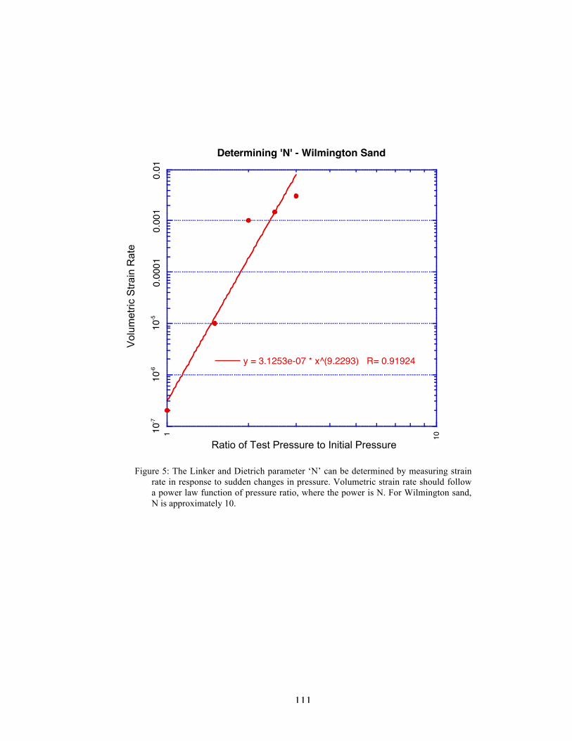
111

Figure 5: The Linker and Dietrich parameter ‘N’ can be determined by measuring strainrate in response to sudden changes in pressure. Volumetric strain rate should followa power law function of pressure ratio, where the power is N. For Wilmington sand,N is approximately 10.

10-7

10-6

10-5

0.00

010.

001

0.01

1 10

Determining 'N' - Wilmington Sand

y = 3.1253e-07 * x^(9.2293) R= 0.91924

Vol

umet

ric S

trai

n R

ate

Ratio of Test Pressure to Initial Pressure

112

Figure B-1: Effect of initial loading rate on the value of the rate-and-state parameter Ce.Ce decreases as inital loading rate increases. For the range of loading rates used here,Ce can be seen to decrease by nearly an order of magnitude.

10-1

010

-910

-810

-710

-610

-5

0.04

0.04

1

0.04

2

0.04

3

0.04

4

0.04

5

0.04

6

0.04

7

0.04

8

Effects of Initial Loading Rate on CompactionUnconsolidated Wilmington Sand

10-7 MPa/s

10-2 MPa/s

Vol

umet

ric S

trai

n R

ate

Volumetric Strain

Ce=18x10

-4

Ce=5x10

-4

113

CHAPTER 5

COMPARING TIME-DEPENDENT END-CAP AND

RATE-AND-STATE FRICTION MODELS

ABSTRACT

Previous studies have shown that creep strain in unconsolidated sands can be

described using both time-dependent end-cap (viscoplastic) and modified rate-and-state

friction models. While these two classes of models are not typically thought of in the

same context, they are qualitatively similar. Each describes stress as a function of state,

strain-rate, and a friction coefficient. In addition, both models originate from empirical

laboratory studies of granular materials. In this chapter, I show that these two models are

also mathematically similar. As the procedure for comparing the two models involves

writing each of them in terms of appropriate stress and strain invariants, a full three-

dimensional formulation of the rate-and-state equations is also provided. I conclude that

the two models are mathematically similar under constant-state boundary conditions.

INTRODUCTION

Rate-and-state friction theory was developed from laboratory observations of the

sliding friction of rocks during shearing (e.g. Ruina, 1983). Laboratory studies (e.g.

Dietrich, 1978; Marone and Scholz, 1989; Byerlee, 1990; Lockner, 1998; Kilgore et al.,

1993) have produced observations that the dynamic coefficient of friction of fractured

rock and gouge varies as a function of both shearing velocity (rate) and the evolution of

damage in the material (state). Both the rate and state terms are modified by multipliers

which have been experimentally determined to have small values (e.g. Linker and

Dietrich, 1992; Marone, 1998). The state variable does not have an exact physical basis,

but is thought to represent the area of contact between slip surfaces (e.g. Kilgore et al.,

1993) or porosity (Segall and Rice,1995; Sleep, 1997). Recent theoretical work by Sleep

(1997, 1999, 2002) has revealed that rate-and-state friction can be used to model the

deformation of intact rock, and that the state variable can be related to strain localization

in a sheared gouge. Recent applications of rate-and-state theory have focused on

modeling earthquake cycles on large faults and predicting the ‘clock advance’ on faults

associated with stress transfer from slip events on nearby faults.

114

Time-dependent end cap models were derived in the mathematics community in

the 1950s (e.g. Drucker, 1950; Perzyna, 1967) as part of the development of plasticity

theory. These models were confirmed experimentally shortly thereafter by the Cambridge

group (Roscoe, 1953; Hvorslev, 1969) for clays and soils. These experiments resulted in

the Cambridge clay models, which simplified the plasticity theory of Drager and

combined it with the concept of critical state soil mechanics (Roscoe, 1953). Simply put,

critical state theory proposes that a material will deform by compaction and shear until it

reaches a critical state at which compaction ceases and all further deformation is taken up

by shearing. Critical state models such as the Cambridge clay have been experimentally

proven to describe a variety of earth materials under a range of stresses and boundary

conditions.

End cap models were developed to describe the behavior of soils and clays using

quantities relevant to conventional triaxial and consolidation tests. Rate-and-state theory

was developed to describe the coefficient of sliding friction of hard rocks using quantities

relevant to direct (simple) shearing tests. Although the rate-and-state and time-dependent

end cap models were developed for different materials, different boundary conditions,

and with different applications in mind, upon comparison they are qualitatively similar.

Both model stress as a function of state (porosity), strain rate, and a friction coefficient.

Both successfully describe the time-dependent compaction of unconsolidated sand at

moderate pressures (Chapters 3 and 4). Based on these qualitative similarities, it is not

too much of a stretch to anticipate that these models are describing the same underlying

physical processes and are mathematically equivalent.

In this paper I show that rate-and-state and time-dependent end cap models are

mathematically similar under constant-state boundary conditions. The basic procedure is

to expand each model to appropriate stress and strain invariants, find complementary

invariants between the two models, and then show their similarity for some set of

assumptions. No attempt is made to rigorously prove that the two models are equivalent.

Rather, the point is merely to show that both models have the same functional form. I

start with the modified Cambridge clay end cap model since derivations exist elsewhere

and then expand the rate-and-state model to three dimensions. Since the two models are

in different two-dimensional coordinate spaces reflecting different boundary conditions,

it is also necessary to find appropriate conditions for comparing them.

115

THEORY PART 1: TIME-DEPENDENT END CAP MODELS AND STRESS

INVARIANTS

End cap models such as the modified Cambridge clay used in this study have been

derived and discussed at length in the plasticity and engineering literature (e.g. Desai and

Siriwardane, 1984); only the equations needed for comparison with the rate-and-state

model are provided here. The yield surface for an end cap model can be defined in terms

of the ratio of deviatoric to mean stress (h=q/p) and the work dissipated during plastic

deformation, which for the modified Cam clay was assumed to be a function of both the

deviatoric and volumetric plastic strains. Solving for the ratio of deviatoric to volumetric

strain (x= des/dev) and assuming associated plasticity results in an equation for the yield

surface, since associated plasticity requires that h=1/x. The yield surface for the modified

Cam clay model is,

(1)

where M is a constant, p is the effective mean stress, p0 is the elastic-plastic transition

pressure, and q is the differential stress. Equation 1 describes an elliptical surface in p-q

stress space. In terms of stress invariants, Equation 1 becomes,

(2)

where J1 is the first invariant of the stress tensor, J10 is the invariant equivalent of p0, and

J2D is the second invariant of the deviatoric stress tensor. For more details and a full

derivation, see the Desai and Siriwardane (1984) chapter on advanced plasticity models.

Next, rate-dependence can be added to the static end cap described by Equations 1

and 2 in the form of viscoplasticity. Perzyna viscoplasticity (1967) is assumed here

because it has been demonstrated to describe the time-dependent compaction of

unconsolidated sands and clays (Adachi and Oka, 1982, Chapter 3). Perzyna assumed

that there was a power law relationship between stress and strain rate during plastic

deformation.

For tests conducted in a conventional triaxial cell, it is convenient to assume that

M is constant and measure J1o as a function of strain rate, so the power law viscoplastic

equation is included in the J1 terms,

(3)

†

M 2 p2 - M2 ppo + q2 = 0,

†

M 2J12 - M2J1J1o + 27J2D = 0,

†

J1vp = J1o + ˙ e ˙ e o( )

1m ,

116

where m is an empirical constant,

†

˙ e o is a reference strain rate, J10 is defined at zero strain

rate, and J1vp is the modified term to be substituted in for J1 terms in Equation 2. Note

that J10 is difficult to measure in practice. On the other hand, tests performed using a

double-direct shear machine typically measure M (approximately 2*m, the coefficient of

friction) as a function of strain rate while holding J1 constant, which means incorporating

the viscoplastic equation into the M terms,

(4)

and substituting Mvp for M in Equation 2. The modified Mvp version of Equation 2 will be

used here for the sake of easier comparison to the rate-and-state equations.

THEORY PART 2: RATE-AND-STATE FRICTION AND STRESS INVARIANTS

Following the notation of Sleep et al. (2000), the rate-and-state friction equation

can be written in terms of strain rate, in which case the shear traction is given by,

(5)

where mo is the steady state coefficient of sliding friction,

†

˙ e is the engineering shear

strain rate, y is the state variable, yo is the normalized value of state, and a and b are

small dimensionless constants. Equation 5 needs to be rewritten in terms of stress and

strain invariants before it can be compared with Equation 2 above. The invariants must be

carefully chosen such that Equation 5 and the engineering shear strain are recovered

when direct (simple) shear stress is applied.

The appropriate strain invariant is found by breaking the strain tensor into

isotropic and deviatoric parts and then manipulating the deviatoric part until the

engineering shear strain is recovered. This was done in the previous chapter when

expanding the rate-and-state slowness equation to include hydrostatic stress boundary

conditions, and so will not be repeated here. The appropriate deviatoric strain invariant

was found to be

(6)

where

†

˙ e ij is the full strain rate tensor,

†

˙ e i˙ j is the deviatoric strain rate tensor, and

†

˙ E is the

engineering shear strain rate. In addition, assuming that changes in state reflect changes

in porosity (Segall and Rice, 1995; Sleep, 1997), the normal compaction (e33) was shown

†

Mvp = M + ˙ e ˙ e o( )

1m,

†

t = sn mo + aln ˙ e ˙ e o( ) + bln y

y o( )[ ],

†

˙ e ij = ˙ E = 2˙ e i˙ j ˙ e i˙ j ,

117

to be equivalent to the volumetric compaction (eii), and eii was selected to be the isotropic

strain invariant.

The stress invariants can be found by manipulating the isotropic and deviatoric

parts of the full stress tensor until Equation 5 is recovered, but J1 and J2D are chosen here

to allow comparison with the time-dependent end cap equation (Equation 2). The first

step is to verify that J1 and J2D satisfy Equation 5 under simple shear stress conditions.

The next step is to verify that the chosen stress and strain rate invariants reduce to

differential stress and strain rate (e.g. s11-s33) for conventional triaxial boundary

conditions, to ensure compatibility with the time-dependent end cap equation, since end

cap experiments are typically conducted under triaxial boundary conditions. Figure 1

shows the appropriate boundary conditions for typical double-direct shear and

conventional triaxial testing machines. If the chosen invariants satisfy both of the above

conditions, then they are correct for this application and a meaningful comparison

between Equations 2 and 5 can be made.

Stress Invariants under direct shear boundary conditions

For direct (simple) shear boundary conditions typically applied in the laboratory,

the only stresses acting on a sample are a single shear traction and a normal traction

perpendicular to the direction of shear, for example,

(7)

where t23=t and s33=sn from Equation 5. Breaking the tensor into spherical (P) and

deviatoric (T) parts and calculating J1 and J2D yields,

(8)

†

0 0 00 0 t23

0 0 s 33

È

Î

Í Í Í

˘

˚

˙ ˙ ˙ ,

†

P =

13 s 33 0 0

0 13 s 33 0

0 0 13 s33

,

J1 = s 33,

T =

- 13 s 33 0 00 - 1

3 s 33 t23

0 t3223 s 33

,

J2D = 12 TijTij = T23

2 + 13 s 33

2 .

118

Substituting J1 for sn, J2D for t, and the appropriate strain rate invariants (mentioned

above) for the shear strain and state variables in Equation 5 reveals that these invariants

are the correct choices, in that Equation 5 is recovered under direct shear conditions, with

one caveat -- J2D contains a normal traction term. As the left side of Equation 5 only

contains shear traction terms, and J2D contains both shear and normal traction terms, it

would appear that the wrong choice has been made. However, while the shear and normal

stresses applied to a sample at the laboratory scale can be completely decoupled, these

stresses cannot be physically decoupled at the grain scale (Although studies of wetted

gouge conducted by Frye and Marone (2002) suggest near complete decoupling at the

grain scale).

The correctness of the invariants posed in Equations 7 and 8 is based upon a

number of assumptions. First, I assumed that describing the gouge using applied tractions

is appropriate. It should be noted that assuming constant-strain boundary conditions

(e11=e22=0) and inferring the stresses in the gouge is probably more similar to double-

direct shear boundary conditions. However, using constant-strain boundary conditions

introduces Poisson’s ratio into s11 and s22, which is problematic because it is unknown.

As adding the Poisson’s ratio terms increases the complexity and clouds the final result of

the following derivation without significantly changing the form of the result, the simpler

imposed-stress boundary conditions will be used.

In addition, the choice of boundary conditions should not matter for small strains,

which are necessary as isotropic stresses and strains are required. The use of invariants

requires nearly isotropic stress and strain conditions in the gouge. This is hardly the case

in well-developed gouge which has strain localized. Well-developed gouge is better

described using anisotropic stress and strain tensors (Sleep, 1998). While Lockner and

Beeler (2003) have recently shown that isotropic rocks become anisotropic with the

application of any deviatoric stress, the assumption of isotropic behavior is probably

valid for an intact material undergoing compaction with a small amount of shear.

Stress Invariants under conventional triaxial boundary conditions

For a conventional triaxial press, there is one axial stress and one radial stress

acting on a cylindrical sample, with principal stresses s11>s22=s33, where s11 is the axial

stress. Dividing the two principal stresses into spherical and deviatoric parts and

calculating J1 and J2D results in

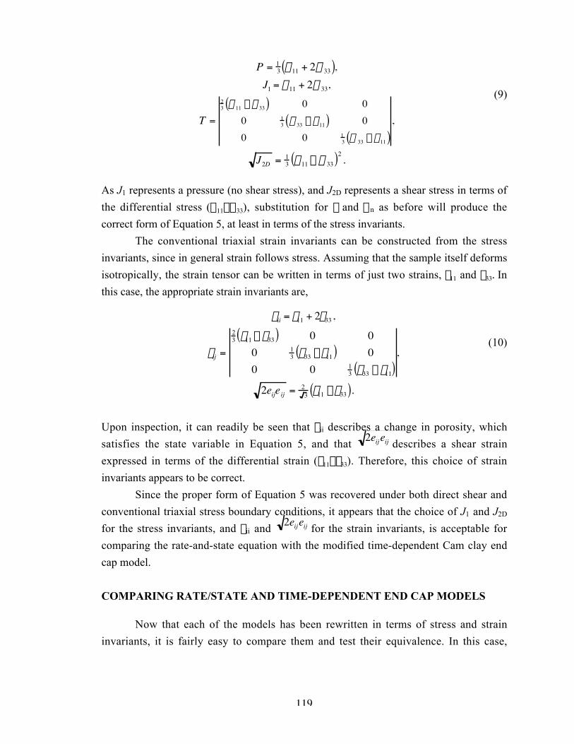
119

(9)

As J1 represents a pressure (no shear stress), and J2D represents a shear stress in terms of

the differential stress (s11-s33), substitution for t and sn as before will produce the

correct form of Equation 5, at least in terms of the stress invariants.

The conventional triaxial strain invariants can be constructed from the stress

invariants, since in general strain follows stress. Assuming that the sample itself deforms

isotropically, the strain tensor can be written in terms of just two strains, e11 and e33. In

this case, the appropriate strain invariants are,

(10)

Upon inspection, it can readily be seen that eii describes a change in porosity, which

satisfies the state variable in Equation 5, and that

†

2eijeij describes a shear strain

expressed in terms of the differential strain (e11-e33). Therefore, this choice of strain

invariants appears to be correct.

Since the proper form of Equation 5 was recovered under both direct shear and

conventional triaxial stress boundary conditions, it appears that the choice of J1 and J2D

for the stress invariants, and eii and

†

2eijeij for the strain invariants, is acceptable for

comparing the rate-and-state equation with the modified time-dependent Cam clay end

cap model.

COMPARING RATE/STATE AND TIME-DEPENDENT END CAP MODELS

Now that each of the models has been rewritten in terms of stress and strain

invariants, it is fairly easy to compare them and test their equivalence. In this case,

†

P = 13 s11 + 2s 33( ),

J1 = s11 + 2s 33,

T =

23 s 11 - s 33( ) 0 0

0 13 s 33 - s11( ) 0

0 0 13 s 33 - s11( )

,

J2D = 13 s11 - s 33( )2 .

†

e ii = e11 + 2e33 ,

eij =

23 e11 - e33( ) 0 0

0 13 e33 -e11( ) 0

0 0 13 e33 - e11( )

,

2eijeij = 23 e11 -e33( ).

120

solving for J2D seems the most direct approach. Starting with the time-dependent

modified Cam clay model, solving for J2D in Equation 2 yields

(11)

and incorporating the time-dependence (Equation 4) into the M terms results in,

(12)

where M o is a reference value measured at the reference strain rate eo. Some

simplification of the M terms yields the final version of the equation,

(13)

which is equal to zero when J1o=J1 or J1=0.

Expressing the time-dependent viscoplasticity in terms of M rather than J1o was

selected deliberately in an attempt to more closely match the end cap equation with the

rate-and-state equation. In a typical direct shear test, the normal stress (J1) is held

constant and the friction coefficient (~M) is observed as a function of strain rate, and

these conditions were matched as closely in the modified end cap model. Likewise,

realizing that an “end cap” represents a yield envelope in stress space at a given constant

porosity, and hence a constant state, the state terms can be eliminated from the rate-and-

state equation for the sake of comparison with the end cap model. Rewriting Equation 5

in terms of J1 and J2D, and eliminating the state terms, results in

(14)

where M is approximately equal to 1/2m and should be equal to Mo in Equation 13, and

†

˙ e o

is a reference strain rate at y=1 and is not necessarily equal to the

†

˙ e o in Equation 13.

Comparing Equations 13 and 14 reveals that they are remarkably similar. They

have the same parabolic functional form, J2D=kJ12, where k contains the M and strain rate

terms and are assumed to be constants or discretely changing variables. Equation 13 has a

power law dependence on strain rate, while Equation 14 follows a logarithmic function of

strain rate. At first this appears to be a difference between the two models, but it is almost

impossible to distinguish between a power law and a logarithmic function over small

windows of observation. In other words, both models should map out the same curve as a

function of strain rate if strain rate only varies by a few orders of magnitude.

†

J2D =1

27 M2J1J1o - M2J12( ),

†

J2D =1

27 J1J1o - J12( ) Mo + ( ˙ e

˙ e o )1m

Ê

Ë Á ˆ

¯ ˜

2

,

†

J2D =J1

27 Mo2 J1o - J1( ) + 2Mo

˙ e ˙ e o

Ê

Ë Á ˆ

¯ ˜

1m

J1o - J1( ) +˙ e ˙ e o

Ê

Ë Á ˆ

¯ ˜

2m

J1o - J1( )È

Î

Í Í Í

˘

˚

˙ ˙ ˙

†

J2D = J12 1

4 M 2 + 12 aM ln ˙ e

˙ e o( ) + aln ˙ e ˙ e o( )( )2È

Î Í ˘ ˚ ˙

121

Figure 2 shows that the two models each have a parabolic form, and that either

one can be empirically scaled such that both are equivalent. Values for the constants are

selected based on available data; m was set equal to 10 (as determined in the previous

chapter), M was set equal to 1 (based on a sliding coefficient of friction of 0.6), and the

strain rate ratio was varied between 0.1 and 10 (values commonly used during slide-hold

tests). In the figure, the time-dependent end cap model is empirically scaled to trace the

rate-and-state model by using a scaling factor of 9/16.

On the other hand, several real differences exist between the two models. The

time-dependent end cap equation (Eq. 13) retains the J10 term which serves as a reference

pressure to define the end cap. The rate-and-state equation (Eq. 14) does not show this

type of dependence on a reference pressure. The reference pressure can be eliminated

from Equation 13, which removes the end cap component of the equation and leaves a

function which simply represents the slope of the critical state line (M) in J1-J2D space,

(15)

This results in an equation almost identical to Equation 14, because the rate-and-state

model simply maps out changes in the coefficient of sliding friction, which is similar to

M, and does not include an end cap component.

A more significant difference exists in the presence of the a terms in Equation 14,

since the last 2 terms in Equations 13 and 15 do not include any weighting factors. Given

that a has been experimentally determined to be on the order of 0.005, this makes the two

models quantitatively different even though they have the same functional form. On the

other hand, a was measured under two-dimensional direct shear loading conditions, and

its value may change under three-dimensional loading conditions. Furthermore, a

weighting parameter like a may exist in Equations 13 and 15 as well; to my knowledge

data to support or refute this is not available.

DISCUSSION

The mathematical similarity between the time-dependent end cap model and the

rate-and-state model has several significant implications. One has to do with the typical

applications that each model is used for. Rate-and-state models can now be used in

typical end cap applications such as geomechanics. Another implication involves the

underlying mechanics of granular materials that the models represent.

Since the models are mathematically related, they should be interchangeable, and

choosing a model for a particular application becomes largely a matter of convenience.†

J2D =J1

2

9 M2 + 2M ˙ e ˙ e o( )

1m

+ ˙ e ˙ e o( )

2mÈ

Î Í ˘ ˚ ˙ .

122

For example, the rate-and-state equation can describe the compaction and deformation of

reservoirs and aquifers. The rate-and-state model can be used to relate changes in

pressure to changes in porosity and the rate of porosity change. The rate-and-state model

can simultaneously be used to predict the slip and compaction of any reservoir bounding

faults, which means that a single model can be used to predict both slip on faults and

compaction in reservoirs simultaneously. On the other hand, the time-dependent end cap

models might be used to study earthquake mechanics, aftershock sequences, and stress

triggering. The presence of an end cap might also help to explain earthquake sequences

and steady state creeping on faults. End cap models would predict that fault-normal

compaction following an earthquake would strengthen the fault and increase the

recurrence time, for example. End cap models also allow for aseismic creep and seismic

slip events to occur on the same fault; compaction dominated shallow stress paths in p-q

space result in creep, while shear dominated steep stress paths result in slip events.

The traditional rate-and-state model lacks an end cap. This is because the rate-

and-state model assumes that deformation is occurring in the plastic domain. For a typical

rate-and-state test, the gouge has been sheared beyond its peak stress and a large amount

of permanent shear deformation has occurred. In other words, the “end cap” has already

been reached. An end cap could be included in the rate-and-state model if the model were

expanded to include elastic deformation and the transition between the elastic and plastic

domains.

The similarity between the two models also suggests that there is an underlying

physical process represented by both models. A model designed to describe small

changes in friction while shearing two blocks of granite together is related to a model

developed to describe the compaction of clays and soils. This result lends support to the

idea that the rate-and-state parameters reflect some intrinsic material properties of

granular materials and that they are not simply empirical fitting parameters. Sleep has

shown that the a parameter can be derived from first principles; the analysis here adds

further experimental evidence that a describes a physical process. Moreover, it appears

that each model represents a part of a more fundamental, universal model, since each

model had to be restricted to constant-state conditions in order to compare them. Rate,

state, the stress field, and the location of an elastic-plastic end cap in stress-space can all

vary simultaneously in reality, but it is very difficult to do this in any kind of controlled

way in the laboratory.

123

CONCLUSIONS

Previous studies have shown that creep strain in unconsolidated sands can be described

using both time-dependent end-cap (viscoplastic) and modified rate-and-state friction

models. While these two classes of models are not typically thought of in the same

context, they are qualitatively similar. Each describes stress as a function of state, strain-

rate, and a friction coefficient. In addition, both models originate from empirical

laboratory studies of granular materials. The procedure for comparing the two models

involves writing each of them in terms of appropriate stress and strain invariants, In this

case the appropriate stress invariants are J1 and J 2D, with similar strain invariants.

Comparing the two models under constant state conditions reveals that the two models

are mathematically similar and have a parabolic functional form, J2D = kJ12, where k is a

constant containing the friction coefficient and strain rate terms. The lack of certain

weighting terms (like a in the rate-and-state model) in the end cap model prevents the

two models from being mathematically equivalent. On the other hand, the fact that the

two models have the same functional form is significant, given that each model was

designed empirically to fit data coming from vastly different materials under different

loading conditions.

REFERENCES

Adachi, T., and Oka, F., 1982, Constitutive equations for normally consolidated claysbased on elasto-viscoplasticity, Soils and Foundations, 22, 4, 57-70.

Blanpied, M.L., Lockner, D.A., and Byerlee, J.D., 1991, Fault stability inferred fromgranite sliding experiments at hydrothermal conditions, Geophys. Res. Letters, 18,609-612.

Byerlee, J., 1990, Friction, overpressure, and fault normal compression, GeophysicsResearch Letters, 17, 2109-2112.

Desai, C.S., and Siriwardane, H.J., 1984, Constitutive Laws for Engineering Materialswith Emphasis on Geologic Materials, Prentice Hall, New Jersey.

Dieterich, J.H., 1978, Time-dependent friction and the mechanics of stick-slip, PureAppl. Geophys., 116, 790-806.

Drucker, D.C., 1950, Some implications of work hardening and ideal plasticity, Quarterlyof Applied Mathematics, 7, 411-418.

Frye, K. M., and C. Marone, 2002,The effect of humidity on granular friction at room temperature, Journal Geophysical Research, 107, doi:10.1029/2001JB000654.

Hvorslev, M.J., 1969, Physical properties of remoulded cohesive soils, Vicksburg, Miss.:US Waterways Experimental Station, 69-5.

Kilgore, B.D., Blanpied, M.L., and Dieterich, J.H., 1993, Velocity dependent friction ofgranite over a wide range of conditions, Geophys. Res. Letters, 20, 903-906.

124

Linker, M.F., and Dieterich, J.H., 1992, Effects of variable normal stress on rock friction:Observations and constitutive equations, J. Geophys. Res., 97, 4923-4940.

Lockner, D.A., 1998, A generalized law for the brittle deformation of Westerly granite,Journal of Geophysics Research, 103, 5107-5123.

Lockner, D.A., and Beeler, N.M., 2003, Stress-induced anisotropic poroelasticityresponse in sandstone, Electronic Proc. 16th ASCE Engin. Mech. Conf., UWashington, Seattle, WA, July 16-18, 2003.

Marone, C., 1998, Effects of loading rate on frictional restrengthening: implications forfault healing and friction constitutive laws, Eos. Trans. AGU, 79(17), S223.

Marone, C., and Scholz, C., 1989, Particle size distribution and microstructures withinsimulated fault gouge, Journal of Structural Geology, 11, 799-814.

Perzyna, P., 1967, Fundamental Problems in Viscoplasticity, Advances in AppliedMechanics, 9, 244-368.

Roscoe, K.H., 1953, An apparatus for the application of simple shear to soil samples,Proc. 3rd Intl. Conference on Soil Mechanics and Foundation Engineering, 1, 186-91.

Ruina, A. 1983, Slip instability and state variable laws, Journal of Geophysics Research,88, 10,359-10,370.

Segall, P., and Rice, J.R., 1995, Dilatancy, compaction, and slip instability of a fluid-infiltrated fault, Journal of Geophysics Research, 100, 22,155-22,171.

Sleep, N.H., 1997, Application of a unified rate and state friction theory to the mechanicsof fault zones with strain localization, Journal of Geophysics Research, 102, 2,875-2,895.

Sleep, N.H., 1998, Rate dependent rate and state friction, Journal of GeophysicsResearch, 103, 7,111-7,119.

Sleep, N.H., 1999, Rate-and-state dependent friction of intact rock and gouge, Journal ofGeophysics Research, 104, 17,847-17,855.

Sleep, N.H., Richardson, E., and Marone, C., 2000, Physics of friction and strain ratelocalization in synthetic fault gouge, Journal of Geophysics Research, 105, B11,25,875-25,890.

Sleep, N.H., 2002, Self-organization of crustal faulting and tectonics, Intl. GeologyReview, 44, 83-96.

125

Figure 1: Comparing typical experimental boundary conditions. In a double-direct shearapparatus, stresses are applied normal and parallel to the fault surface (a), while in aconventional triaxial apparatus, the fault surface exists at some angle to the primarystresses.

t

P s1

s3

a) b)

Double-direct Shear Conventional Triaxial

126

Figure 2: Both the rate-and-state and time-dependent end cap models have the sameparabolic functional form. Both models also show the same increase in J2D at a givenJ1 with increasing strain rate. While the time-dependent end cap model does notexactly trace the rate-and-state model, it can be scaled to do so, as shown by thedotting curve at a strain rate of 1.

0

1000

2000

3000

4000

5000

6000

0 20 40 60 80 100 120

Comparison of Rate-and-State and Time-dependent End Cap Models

rate = 1rate = 1rate = 0.1rate = 0.1rate = 10rate = 10rate = 1

J 2D

J1

Time-dependent End Cap model

Rate-and-State model

Scaled End Cap model is equivalent to Rate and State