J U A N X I N G

C A N A D I A N G R A I N C O M M I S S I O N

APPLICATION OF USING SAS FOR TIME SERIES FORECASTING

TIME SERIES ANALYSIS

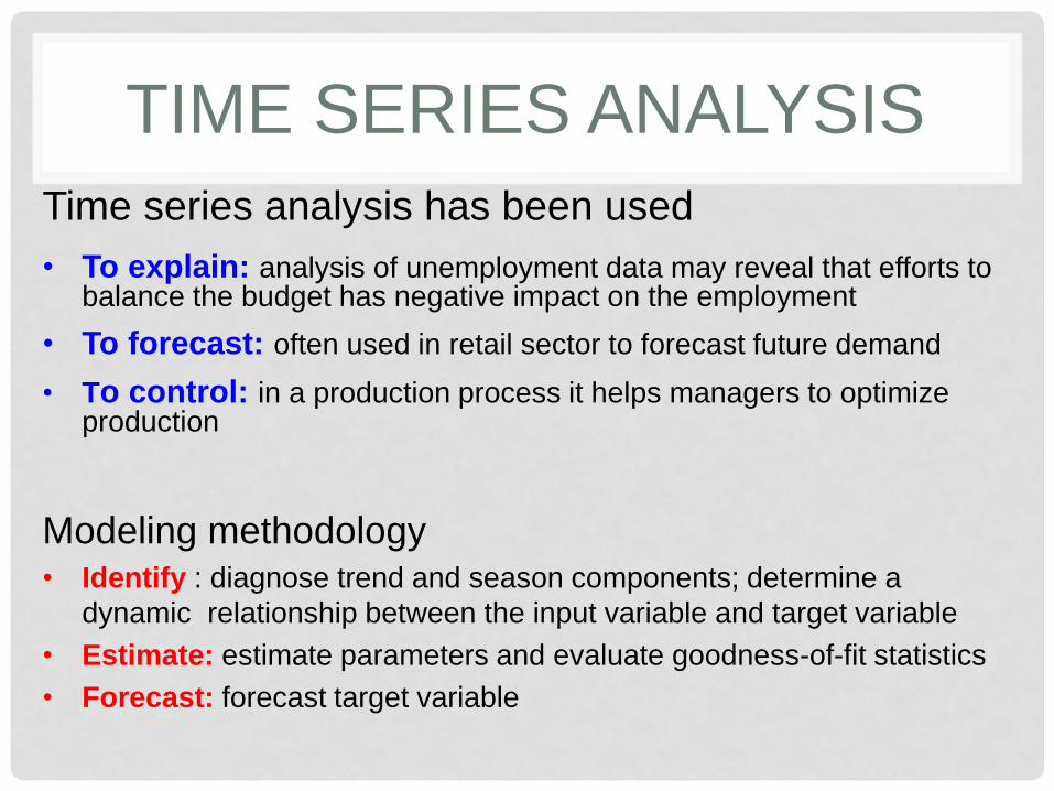
Time series analysis has been used

• To explain: analysis of unemployment data may reveal that efforts to balance the budget has negative impact on the employment

• To forecast: often used in retail sector to forecast future demand

• To control: in a production process it helps managers to optimize production

Modeling methodology• Identify : diagnose trend and season components; determine a

dynamic relationship between the input variable and target variable

• Estimate: estimate parameters and evaluate goodness-of-fit statistics

• Forecast: forecast target variable

A time series may exhibit systematic variations in the form of trend, seasonality and cyclical variation

A time series may also exhibit impact of event(s): economic index, natural disasters, new emerged technology, policy changes, … …

TIME SERIES ANALYSIS

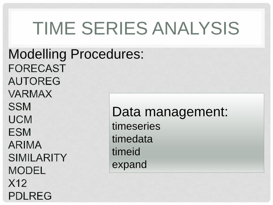
Modelling Procedures:

Data management: timeseries

timedata

timeid

expand

TIME SERIES ANALYSIS

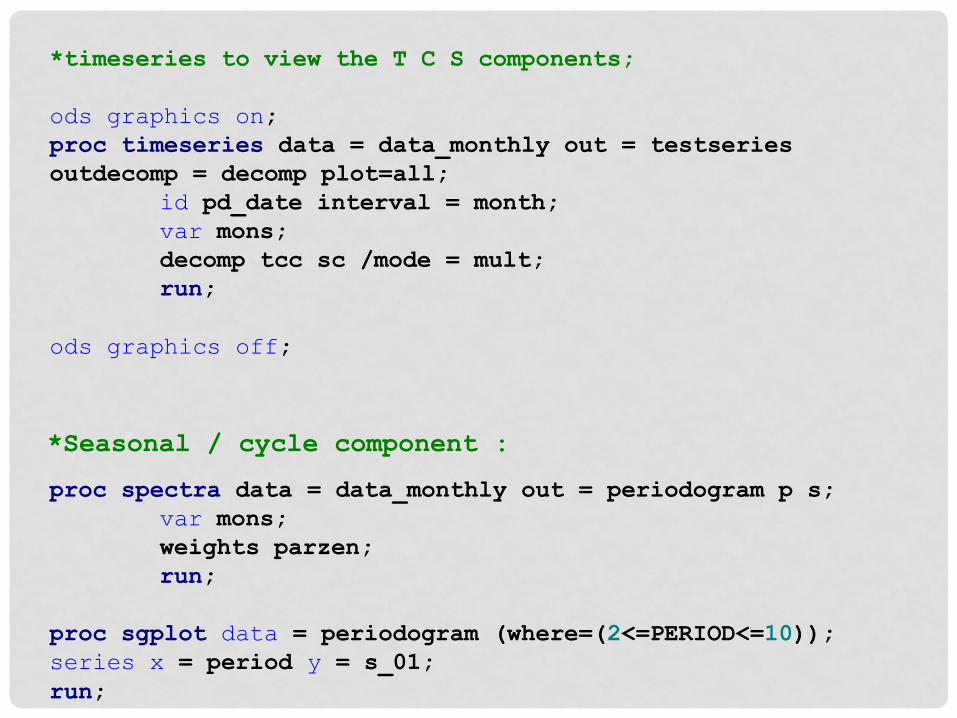
*timeseries to view the T C S components;

ods graphics on;

proc timeseries data = data_monthly out = testseries

outdecomp = decomp plot=all;

id pd_date interval = month;

var mons;

decomp tcc sc /mode = mult;

run;

ods graphics off;

proc spectra data = data_monthly out = periodogram p s;

var mons;

weights parzen;

run;

proc sgplot data = periodogram (where=(2<=PERIOD<=10));

series x = period y = s_01;

run;

*Seasonal / cycle component :

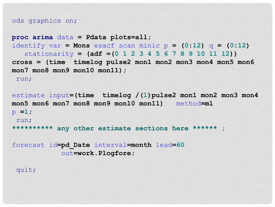
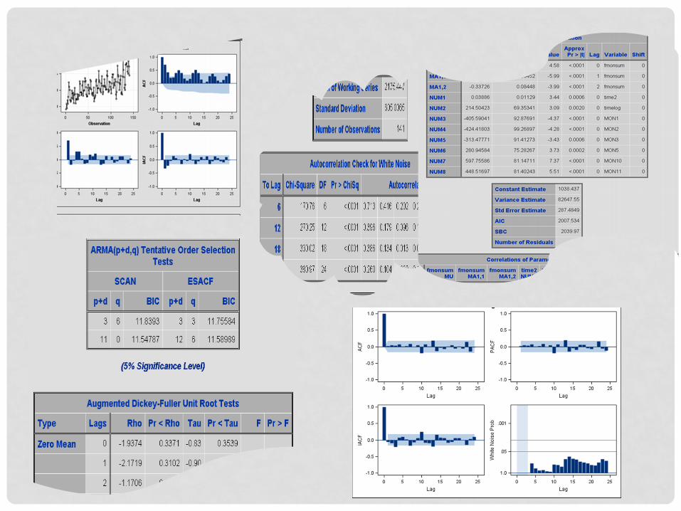
ods graphics on;

proc arima data = Pdata plots=all;

identify var = Mons esacf scan minic p = (0:12) q = (0:12)

stationarity = (adf =(0 1 2 3 4 5 6 7 8 9 10 11 12))

cross = (time timelog pulse2 mon1 mon2 mon3 mon4 mon5 mon6

mon7 mon8 mon9 mon10 mon11);

run;

estimate input=(time timelog /(1)pulse2 mon1 mon2 mon3 mon4

mon5 mon6 mon7 mon8 mon9 mon10 mon11) method=ml

p =1;

run;

********** any other estimate sections here ****** ;

forecast id=pd_Date interval=month lead=60

out=work.Plogfore;

quit;

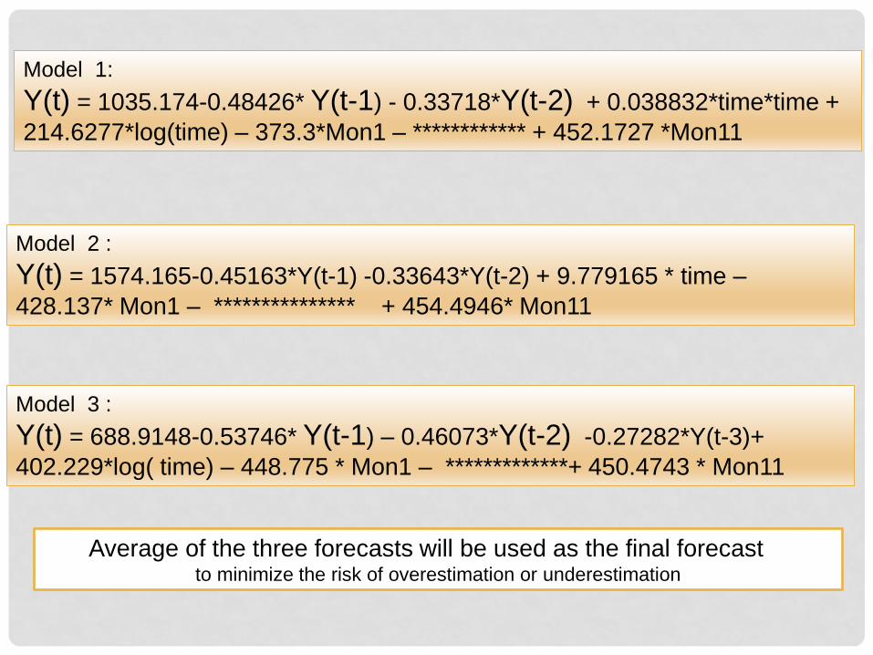
Model 1:

Y(t) = 1035.174-0.48426* Y(t-1) - 0.33718*Y(t-2) + 0.038832*time*time +

214.6277*log(time) – 373.3*Mon1 – ************ + 452.1727 *Mon11

Model 2 :

Y(t) = 1574.165-0.45163*Y(t-1) -0.33643*Y(t-2) + 9.779165 * time –

428.137* Mon1 – *************** + 454.4946* Mon11

Model 3 :

Y(t) = 688.9148-0.53746* Y(t-1) – 0.46073*Y(t-2) -0.27282*Y(t-3)+

402.229*log( time) – 448.775 * Mon1 – *************+ 450.4743 * Mon11

Average of the three forecasts will be used as the final forecast to minimize the risk of overestimation or underestimation

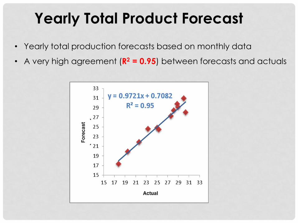
• Yearly total production forecasts based on monthly data

• A very high agreement (R2 = 0.95) between forecasts and actuals

Yearly Total Product Forecast

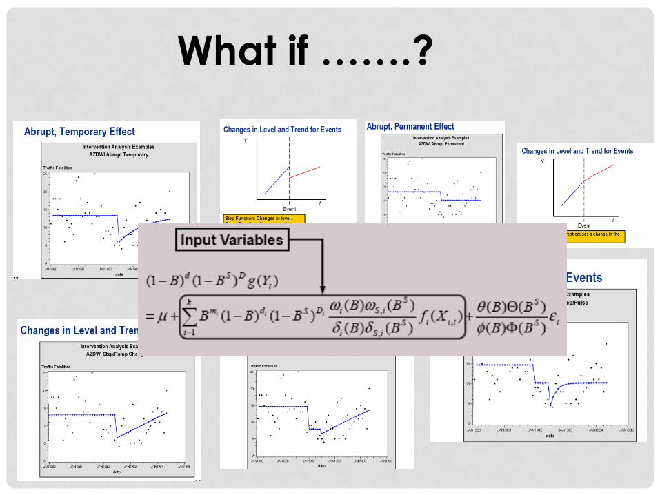
What if …….?

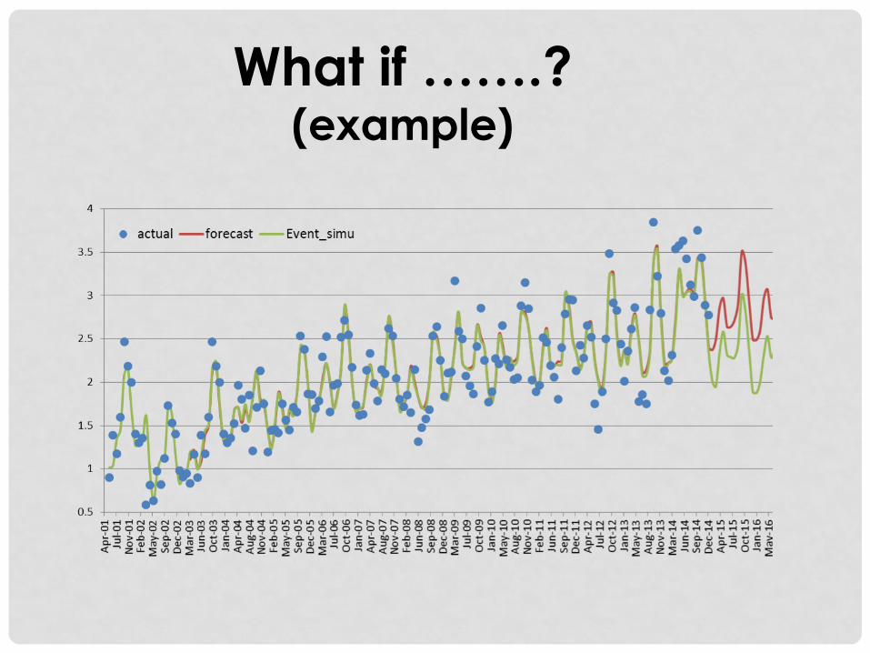
What if …….?(example)

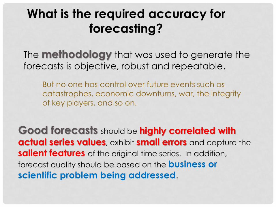
What is the required accuracy for

forecasting?

The methodology that was used to generate the

forecasts is objective, robust and repeatable.

But no one has control over future events such as catastrophes, economic downturns, war, the integrity

of key players, and so on.

Good forecasts should be highly correlated with

actual series values, exhibit small errors and capture the

salient features of the original time series. In addition,

forecast quality should be based on the business or

scientific problem being addressed.

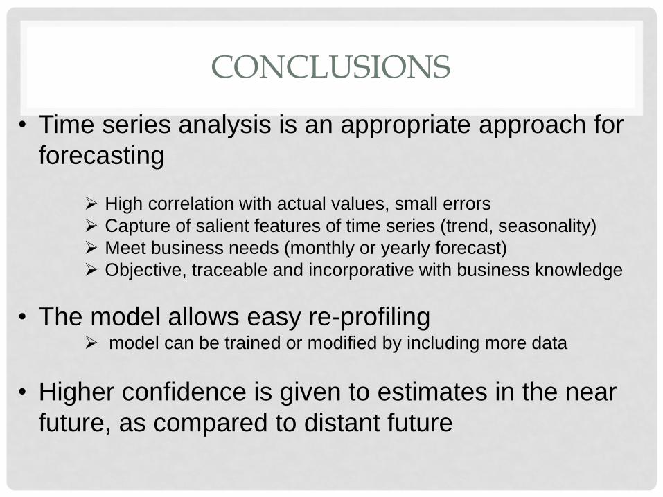
CONCLUSIONS

• Time series analysis is an appropriate approach for

forecasting

High correlation with actual values, small errors

Capture of salient features of time series (trend, seasonality)

Meet business needs (monthly or yearly forecast)

Objective, traceable and incorporative with business knowledge

• The model allows easy re-profiling model can be trained or modified by including more data

• Higher confidence is given to estimates in the near

future, as compared to distant future

Thank you !