APPLICATION OF THREE-COMPONENT PIV TO A HOVERING ROTOR WAKE

James T. HeineckExperimental Physics BranchNASA Ames Research Center

Moffett Field, CA

Gloria K. YamauchiArmy / NASA Rotorcraft Division

NASA Ames Research CenterMoffett Field, CA

Alan J. WadcockAerospace Computing, Inc.

Los Altos, CA

Luiz LourencoFlorida State/Florida A&M University

Tallahassee, FL

Anita I. AbregoArmy / NASA Rotorcraft Division

NASA Ames Research CenterMoffett Field, CA

Abstract1

Three-component velocity measurements in thewake of a two-bladed rotor in hover were made usingthe Particle Image Velocimetry (PIV) technique. Thevelocity fields were oriented in a plane normal to therotor disk and were acquired for wake ages rangingfrom 0 to 270 deg. for one rotor thrust condition. Theexperimental setup and processing of theinstantaneous images are discussed. Data averagingschemes are demonstrated to mitigate the smearingeffects of vortex wander. The effect of vortex wanderon the measured vortex core size is presented.

Introduction

The key to accurate predictions of rotorcraftaerodynamics, acoustics, and dynamics lies in theaccurate representation of the rotor wake. The vorticalwakes computed by rotorcraft CFD analyses typicallysuffer from numerical dissipation before the first bladepassage. With some a priori knowledge of the waketrajectory, grid points can be concentrated along thetrajectory to minimize this dissipation.Comprehensive rotorcraft analyses based on lifting-line theory rely on classical vortex models and/orsemi-empirical information about the tip vortexstructure. Until the location, size, and strength of thetrailed tip vortex can be measured over a range of

Presented at the American Helicopter Society 56thAnnual Forum, Virginia Beach, Virginia, May 2-4,2000. Copyright © 2000 by the American HelicopterSociety, Inc. All rights reserved.

wake ages, the analyses will continue to be adjustedon a trial and error basis to correctly predict bladeairloads, acoustics, dynamics, and performance. Usingthe laser light sheet technique, tip vortex location canbe acquired in a straightforward manner. Measuringwake velocities and vortex core size, however, hasbeen difficult and tedious using point-measurementtechniques such as laser velocimetry. The ParticleImage Velocimetry (PIV) technique has proven to bean efficient method for acquiring velocitymeasurements over relatively large areas and volumesfor rotating flow-fields. The majority of PIV workreported to date has been restricted to 2-componentvelocity measurements acquired from the wake of arotor in forward flight (Refs. 1-12). Ref. 10 describesan experiment where three-component velocitymeasurements were made on a rotor in forward flight,although only preliminary results are shown.Although PIV has become an increasingly favoredtechnique for acquiring flow field information on rotorwakes, there has been minimal information in theliterature regarding methods of extracting criticalparameters such as vortex core size and strength fromPIV data.

The present work had two objectives. The firstobjective was to gain experience in applying thethree-component (3D) PIV technique to a simple rotorconfiguration. A two-bladed, untwisted rotoroperating at moderate thrust in hover was selected forthis investigation. Restricting the test conditions tohover allowed greater freedom, compared to forwardflight testing, in locating the cameras and laser sheet.Three-component PIV permits both cameras to bepositioned in the forward scatter position relative tothe laser light sheet thereby maximizing the qualityof the particle images. The second objective was to

obtain vortex core size and document the effects ofvortex wander.

This paper provides a description of the testfacility and the model used for the experiment, adiscussion of the test conditions, a detailed descriptionof the PIV measurement set-up, and the dataprocessing technique and procedures. Specific findingsfrom this experiment are discussed.

Facility and Model Description

The experiment was performed at NASA AmesResearch Center in the U.S. ArmyAeroflightdynamics Directorate Hover Test Chamber.The following sections describe the test chamber androtor model.

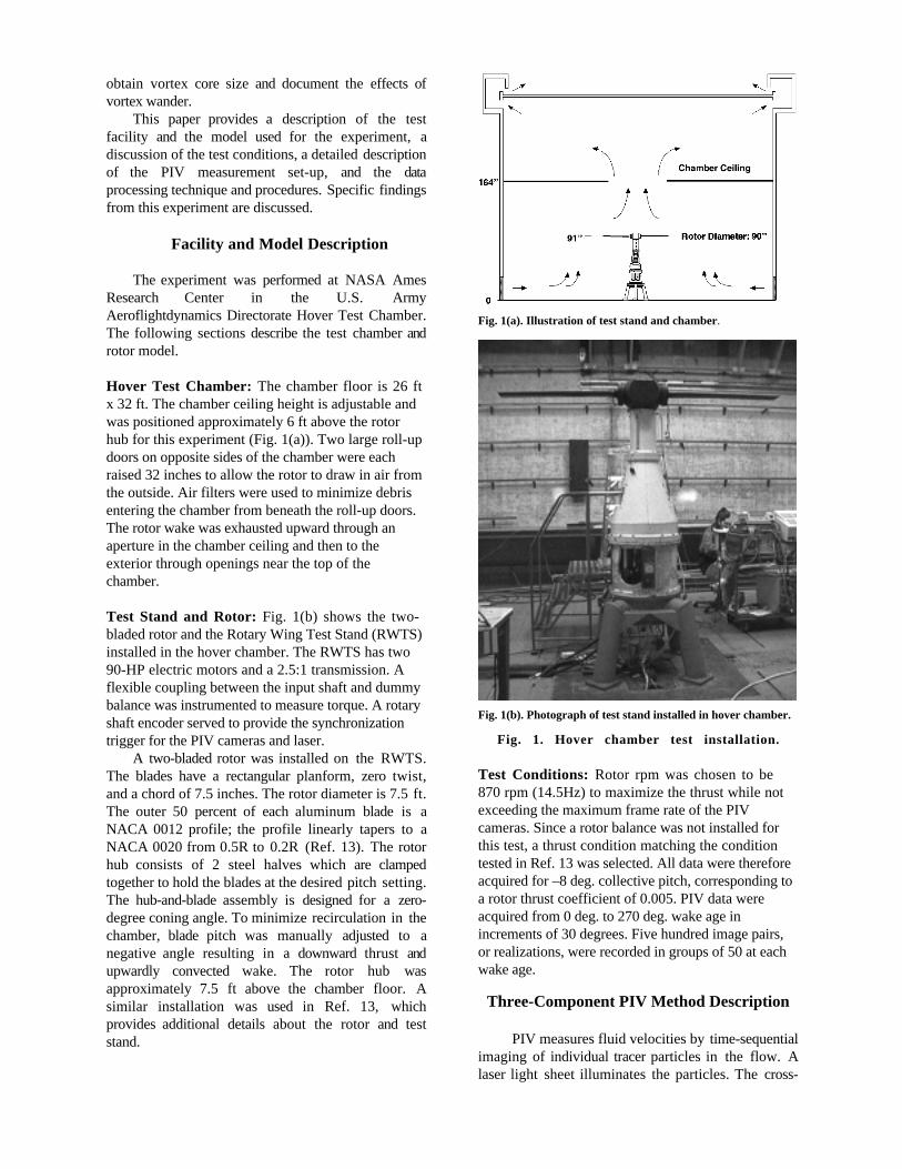
Hover Test Chamber: The chamber floor is 26 ftx 32 ft. The chamber ceiling height is adjustable andwas positioned approximately 6 ft above the rotorhub for this experiment (Fig. 1(a)). Two large roll-updoors on opposite sides of the chamber were eachraised 32 inches to allow the rotor to draw in air fromthe outside. Air filters were used to minimize debrisentering the chamber from beneath the roll-up doors.The rotor wake was exhausted upward through anaperture in the chamber ceiling and then to theexterior through openings near the top of thechamber.

Test Stand and Rotor: Fig. 1(b) shows the two-bladed rotor and the Rotary Wing Test Stand (RWTS)installed in the hover chamber. The RWTS has two90-HP electric motors and a 2.5:1 transmission. Aflexible coupling between the input shaft and dummybalance was instrumented to measure torque. A rotaryshaft encoder served to provide the synchronizationtrigger for the PIV cameras and laser.

A two-bladed rotor was installed on the RWTS.The blades have a rectangular planform, zero twist,and a chord of 7.5 inches. The rotor diameter is 7.5 ft.The outer 50 percent of each aluminum blade is aNACA 0012 profile; the profile linearly tapers to aNACA 0020 from 0.5R to 0.2R (Ref. 13). The rotorhub consists of 2 steel halves which are clampedtogether to hold the blades at the desired pitch setting.The hub-and-blade assembly is designed for a zero-degree coning angle. To minimize recirculation in thechamber, blade pitch was manually adjusted to anegative angle resulting in a downward thrust andupwardly convected wake. The rotor hub wasapproximately 7.5 ft above the chamber floor. Asimilar installation was used in Ref. 13, whichprovides additional details about the rotor and teststand.

Fig. 1(a). Illustration of test stand and chamber.

Fig. 1(b). Photograph of test stand installed in hover chamber.

Fig. 1. Hover chamber test installation.

Test Conditions: Rotor rpm was chosen to be870 rpm (14.5Hz) to maximize the thrust while notexceeding the maximum frame rate of the PIVcameras. Since a rotor balance was not installed forthis test, a thrust condition matching the conditiontested in Ref. 13 was selected. All data were thereforeacquired for –8 deg. collective pitch, corresponding toa rotor thrust coefficient of 0.005. PIV data wereacquired from 0 deg. to 270 deg. wake age inincrements of 30 degrees. Five hundred image pairs,or realizations, were recorded in groups of 50 at eachwake age.

Three-Component PIV Method Description

PIV measures fluid velocities by time-sequentialimaging of individual tracer particles in the flow. Alaser light sheet illuminates the particles. The cross-

correlation of two successive images yields themagnitude and direction of the particle displacement.

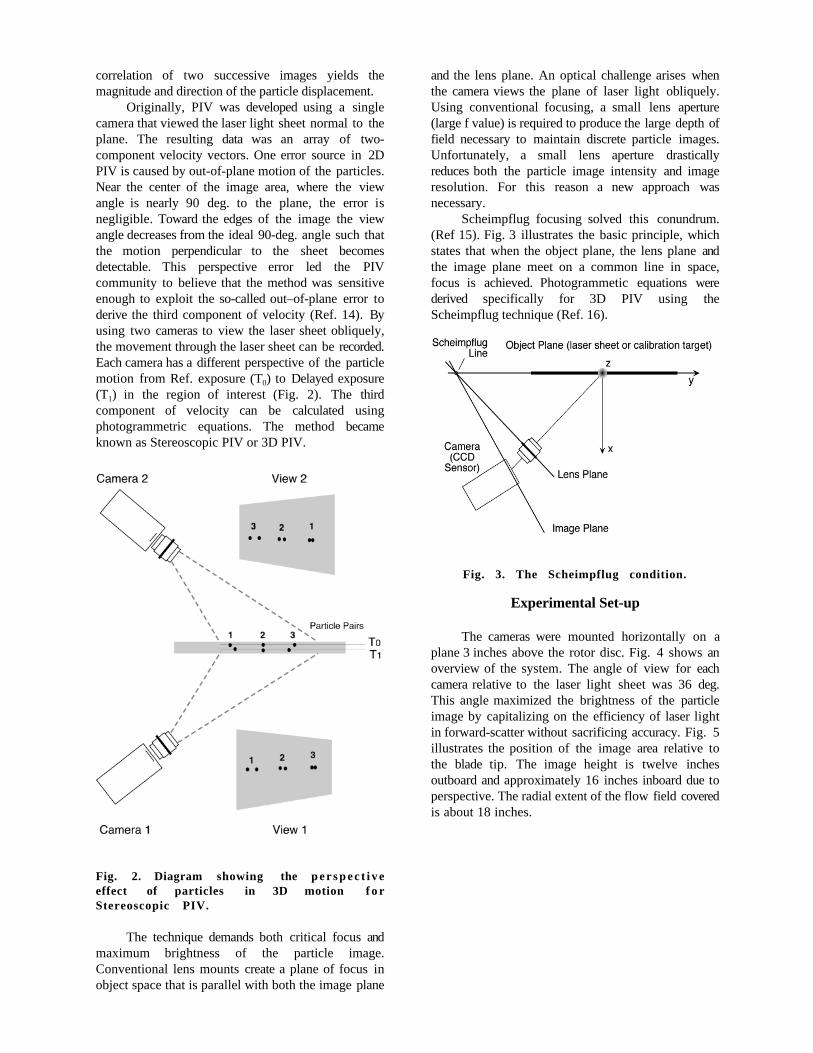
Originally, PIV was developed using a singlecamera that viewed the laser light sheet normal to theplane. The resulting data was an array of two-component velocity vectors. One error source in 2DPIV is caused by out-of-plane motion of the particles.Near the center of the image area, where the viewangle is nearly 90 deg. to the plane, the error isnegligible. Toward the edges of the image the viewangle decreases from the ideal 90-deg. angle such thatthe motion perpendicular to the sheet becomesdetectable. This perspective error led the PIVcommunity to believe that the method was sensitiveenough to exploit the so-called out–of-plane error toderive the third component of velocity (Ref. 14). Byusing two cameras to view the laser sheet obliquely,the movement through the laser sheet can be recorded.Each camera has a different perspective of the particlemotion from Ref. exposure (T0) to Delayed exposure(T1) in the region of interest (Fig. 2). The thirdcomponent of velocity can be calculated usingphotogrammetric equations. The method becameknown as Stereoscopic PIV or 3D PIV.

Fig. 2. Diagram showing the pe rspec t i veeffect of particles in 3D motion f o rStereoscopic PIV.

The technique demands both critical focus andmaximum brightness of the particle image.Conventional lens mounts create a plane of focus inobject space that is parallel with both the image plane

and the lens plane. An optical challenge arises whenthe camera views the plane of laser light obliquely.Using conventional focusing, a small lens aperture(large f value) is required to produce the large depth offield necessary to maintain discrete particle images.Unfortunately, a small lens aperture drasticallyreduces both the particle image intensity and imageresolution. For this reason a new approach wasnecessary.

Scheimpflug focusing solved this conundrum.(Ref 15). Fig. 3 illustrates the basic principle, whichstates that when the object plane, the lens plane andthe image plane meet on a common line in space,focus is achieved. Photogrammetic equations werederived specifically for 3D PIV using theScheimpflug technique (Ref. 16).

Fig. 3. The Scheimpflug condition.

Experimental Set-up

The cameras were mounted horizontally on aplane 3 inches above the rotor disc. Fig. 4 shows anoverview of the system. The angle of view for eachcamera relative to the laser light sheet was 36 deg.This angle maximized the brightness of the particleimage by capitalizing on the efficiency of laser lightin forward-scatter without sacrificing accuracy. Fig. 5illustrates the position of the image area relative tothe blade tip. The image height is twelve inchesoutboard and approximately 16 inches inboard due toperspective. The radial extent of the flow field coveredis about 18 inches.

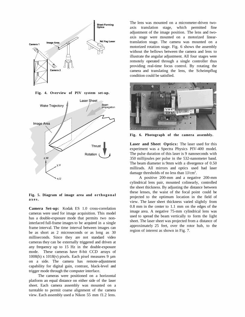
Fig. 4. Overview of PIV system set-up.

Fig. 5. Diagram of image area and o r t hogona la x e s .

Camera Set-up: Kodak ES 1.0 cross-correlationcameras were used for image acquisition. This modelhas a double-exposure mode that permits two non-interlaced full-frame images to be acquired in a singleframe interval. The time interval between images canbe as short as 2 microseconds or as long as 30milliseconds. Since they are not standard videocameras they can be externally triggered and driven atany frequency up to 15 Hz in the double-exposuremode. These cameras have 8-bit CCD arrays of1008(h) x 1018(v) pixels. Each pixel measures 9 µmon a side. The camera has remote-adjustmentcapability for digital gain, contrast, black-level andtrigger mode through the computer interface.

The cameras were positioned on a horizontalplatform an equal distance on either side of the lasersheet. Each camera assembly was mounted on aturntable to permit coarse alignment of the cameraview. Each assembly used a Nikon 55 mm f1.2 lens.

The lens was mounted on a micrometer-driven two-axis translation stage, which permitted fineadjustment of the image position. The lens and two-axis stage were mounted on a motorized linear-translation stage. The camera was mounted on amotorized rotation stage. Fig. 6 shows the assemblywithout the bellows between the camera and lens toillustrate the angular adjustment. All four stages wereremotely operated through a single controller thusproviding real-time focus control. By rotating thecamera and translating the lens, the Scheimpflugcondition could be satisfied.

Fig. 6. Photograph of the camera assembly.

Laser and Sheet Optics: The laser used for thisexperiment was a Spectra Physics PIV-400 model.The pulse duration of this laser is 9 nanoseconds with350 millijoules per pulse in the 532-nanometer band.The beam diameter is 9mm with a divergence of 0.50millirads. All mirrors and optics used had laserdamage thresholds of no less than 1J/cm2.

A positive 200-mm and a negative 200-mmcylindrical lens pair, mounted colinearly, controlledthe sheet thickness. By adjusting the distance betweenthese lenses, the waist of the focal point could beprojected to the optimum location in the field ofview. The laser sheet thickness varied slightly from0.8 mm in the center to 1.1 mm on the edges of theimage area. A negative 75-mm cylindrical lens wasused to spread the beam vertically to form the lightsheet. The laser sheet was projected from a distance ofapproximately 25 feet, over the rotor hub, to theregion of interest as shown in Fig. 7.

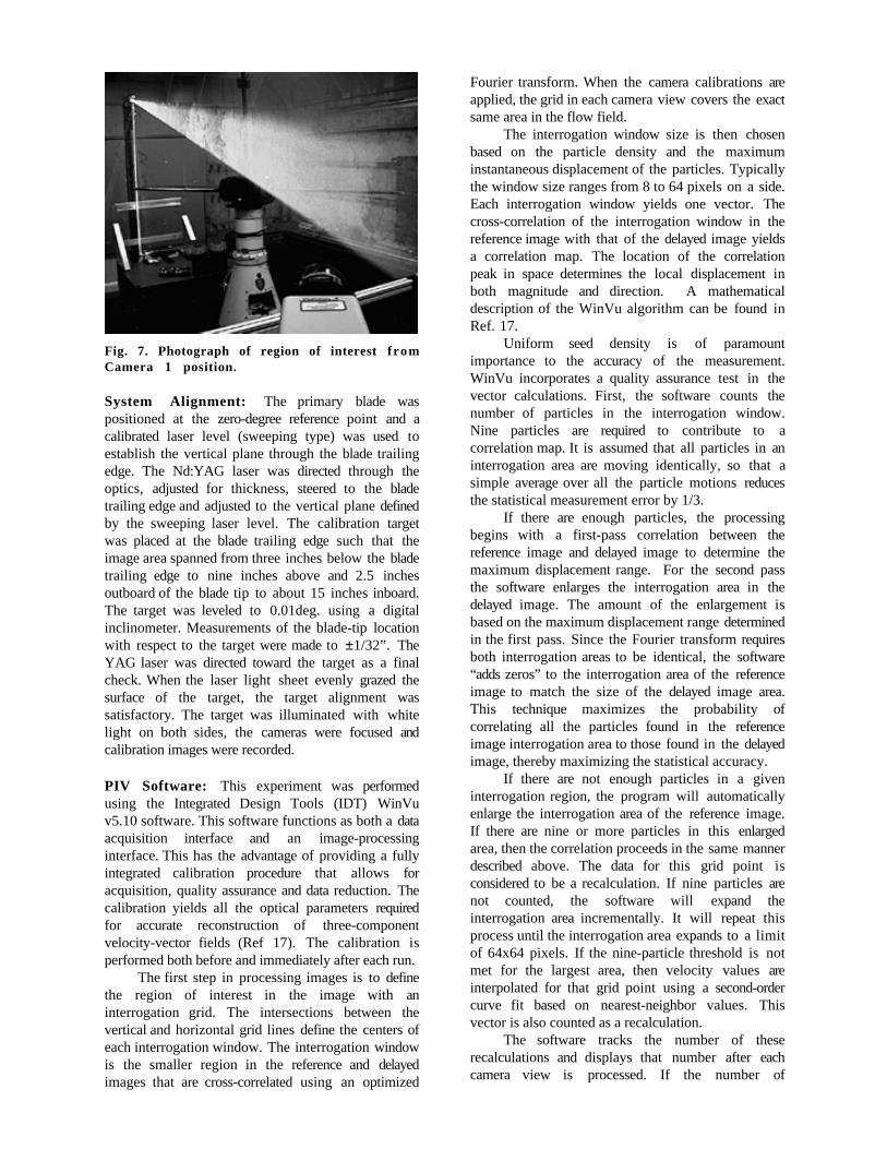
Fig. 7. Photograph of region of interest f romCamera 1 position.

System Alignment: The primary blade waspositioned at the zero-degree reference point and acalibrated laser level (sweeping type) was used toestablish the vertical plane through the blade trailingedge. The Nd:YAG laser was directed through theoptics, adjusted for thickness, steered to the bladetrailing edge and adjusted to the vertical plane definedby the sweeping laser level. The calibration targetwas placed at the blade trailing edge such that theimage area spanned from three inches below the bladetrailing edge to nine inches above and 2.5 inchesoutboard of the blade tip to about 15 inches inboard.The target was leveled to 0.01deg. using a digitalinclinometer. Measurements of the blade-tip locationwith respect to the target were made to ±1/32”. TheYAG laser was directed toward the target as a finalcheck. When the laser light sheet evenly grazed thesurface of the target, the target alignment wassatisfactory. The target was illuminated with whitelight on both sides, the cameras were focused andcalibration images were recorded.

PIV Software: This experiment was performedusing the Integrated Design Tools (IDT) WinVuv5.10 software. This software functions as both a dataacquisition interface and an image-processinginterface. This has the advantage of providing a fullyintegrated calibration procedure that allows foracquisition, quality assurance and data reduction. Thecalibration yields all the optical parameters requiredfor accurate reconstruction of three-componentvelocity-vector fields (Ref 17). The calibration isperformed both before and immediately after each run.

The first step in processing images is to definethe region of interest in the image with aninterrogation grid. The intersections between thevertical and horizontal grid lines define the centers ofeach interrogation window. The interrogation windowis the smaller region in the reference and delayedimages that are cross-correlated using an optimized

Fourier transform. When the camera calibrations areapplied, the grid in each camera view covers the exactsame area in the flow field.

The interrogation window size is then chosenbased on the particle density and the maximuminstantaneous displacement of the particles. Typicallythe window size ranges from 8 to 64 pixels on a side.Each interrogation window yields one vector. Thecross-correlation of the interrogation window in thereference image with that of the delayed image yieldsa correlation map. The location of the correlationpeak in space determines the local displacement inboth magnitude and direction. A mathematicaldescription of the WinVu algorithm can be found inRef. 17.

Uniform seed density is of paramountimportance to the accuracy of the measurement.WinVu incorporates a quality assurance test in thevector calculations. First, the software counts thenumber of particles in the interrogation window.Nine particles are required to contribute to acorrelation map. It is assumed that all particles in aninterrogation area are moving identically, so that asimple average over all the particle motions reducesthe statistical measurement error by 1/3.

If there are enough particles, the processingbegins with a first-pass correlation between thereference image and delayed image to determine themaximum displacement range. For the second passthe software enlarges the interrogation area in thedelayed image. The amount of the enlargement isbased on the maximum displacement range determinedin the first pass. Since the Fourier transform requiresboth interrogation areas to be identical, the software“adds zeros” to the interrogation area of the referenceimage to match the size of the delayed image area.This technique maximizes the probability ofcorrelating all the particles found in the referenceimage interrogation area to those found in the delayedimage, thereby maximizing the statistical accuracy.

If there are not enough particles in a giveninterrogation region, the program will automaticallyenlarge the interrogation area of the reference image.If there are nine or more particles in this enlargedarea, then the correlation proceeds in the same mannerdescribed above. The data for this grid point isconsidered to be a recalculation. If nine particles arenot counted, the software will expand theinterrogation area incrementally. It will repeat thisprocess until the interrogation area expands to a limitof 64x64 pixels. If the nine-particle threshold is notmet for the largest area, then velocity values areinterpolated for that grid point using a second-ordercurve fit based on nearest-neighbor values. Thisvector is also counted as a recalculation.

The software tracks the number of theserecalculations and displays that number after eachcamera view is processed. If the number of

recalculations is less than 1% of the total vectors thenthe data are considered reliable.

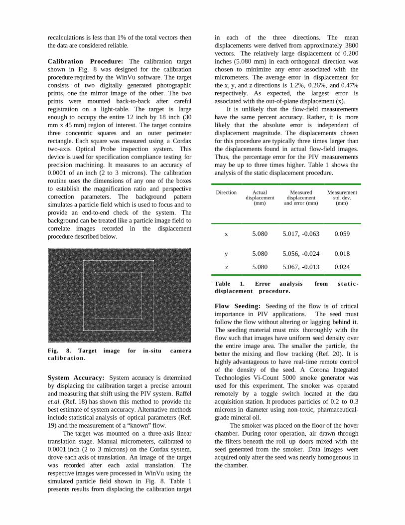
Calibration Procedure: The calibration targetshown in Fig. 8 was designed for the calibrationprocedure required by the WinVu software. The targetconsists of two digitally generated photographicprints, one the mirror image of the other. The twoprints were mounted back-to-back after carefulregistration on a light-table. The target is largeenough to occupy the entire 12 inch by 18 inch (30mm x 45 mm) region of interest. The target containsthree concentric squares and an outer perimeterrectangle. Each square was measured using a Cordaxtwo-axis Optical Probe inspection system. Thisdevice is used for specification compliance testing forprecision machining. It measures to an accuracy of0.0001 of an inch (2 to 3 microns). The calibrationroutine uses the dimensions of any one of the boxesto establish the magnification ratio and perspectivecorrection parameters. The background patternsimulates a particle field which is used to focus and toprovide an end-to-end check of the system. Thebackground can be treated like a particle image field tocorrelate images recorded in the displacementprocedure described below.

Fig. 8. Target image for in-situ cameraca l i b ra t i on .

System Accuracy: System accuracy is determinedby displacing the calibration target a precise amountand measuring that shift using the PIV system. Raffelet.al. (Ref. 18) has shown this method to provide thebest estimate of system accuracy. Alternative methodsinclude statistical analysis of optical parameters (Ref.19) and the measurement of a “known” flow.

The target was mounted on a three-axis lineartranslation stage. Manual micrometers, calibrated to0.0001 inch (2 to 3 microns) on the Cordax system,drove each axis of translation. An image of the targetwas recorded after each axial translation. Therespective images were processed in WinVu using thesimulated particle field shown in Fig. 8. Table 1presents results from displacing the calibration target

in each of the three directions. The meandisplacements were derived from approximately 3800vectors. The relatively large displacement of 0.200inches (5.080 mm) in each orthogonal direction waschosen to minimize any error associated with themicrometers. The average error in displacement forthe x, y, and z directions is 1.2%, 0.26%, and 0.47%respectively. As expected, the largest error isassociated with the out-of-plane displacement (x).

It is unlikely that the flow-field measurementshave the same percent accuracy. Rather, it is morelikely that the absolute error is independent ofdisplacement magnitude. The displacements chosenfor this procedure are typically three times larger thanthe displacements found in actual flow-field images.Thus, the percentage error for the PIV measurementsmay be up to three times higher. Table 1 shows theanalysis of the static displacement procedure.

Direction Actualdisplacement

(mm)

Measureddisplacement

and error (mm)

Measurementstd. dev.(mm)

x 5.080 5.017, -0.063 0.059

y 5.080 5.056, -0.024 0.018

z 5.080 5.067, -0.013 0.024

Table 1. Error analysis from s t a t i c -displacement procedure.

Flow Seeding: Seeding of the flow is of criticalimportance in PIV applications. The seed mustfollow the flow without altering or lagging behind it.The seeding material must mix thoroughly with theflow such that images have uniform seed density overthe entire image area. The smaller the particle, thebetter the mixing and flow tracking (Ref. 20). It ishighly advantageous to have real-time remote controlof the density of the seed. A Corona IntegratedTechnologies Vi-Count 5000 smoke generator wasused for this experiment. The smoker was operatedremotely by a toggle switch located at the dataacquisition station. It produces particles of 0.2 to 0.3microns in diameter using non-toxic, pharmaceutical-grade mineral oil.

The smoker was placed on the floor of the hoverchamber. During rotor operation, air drawn throughthe filters beneath the roll up doors mixed with theseed generated from the smoker. Data images wereacquired only after the seed was nearly homogenous inthe chamber.

Data Acquisition

The PIV cameras were each connected toseparate Imaging Technology IC- PCI frame grabbersinstalled in a PC workstation. Image acquisition wasperformed using WinVu enabling efficient, real-timeassessment of image quality. Sample images wereacquired and processed to optimize image quality andinter-pulse time delay.

A successful PIV measurement is highlydependent on the quality of the raw images. Issuessuch as background light contamination, imagebrightness, contrast, focus, beam alignment and lightpulse separation bear on the success of imagecorrelation.

Fine focusing and beam-alignment wereperformed using a seeded jet prior to testing. The jetwas a small blower whose intake drew from theambient air mixed with the smoke. Focusing wasaccomplished using the remotely operated translationstages while observing the real-time display. The gainand black-level were then adjusted to maximizecontrast and brightness of the particle field. To checkfor laser sheet coplanarity, the motion of the particleswas observed on the real-time display where bothlaser pulses were recorded in one image. As the beamscame into alignment, the particle images appeared asdoublets.

The final parameter, the inter-pulse time delay,has to be determined under actual test conditions.Sample images are acquired and processed in near real-time. Adjustments to the time delay are made basedon the resulting correlation. The most importantinformation required for determining the time delay isthe maximum instantaneous displacement. Itrepresents the highest velocity in the flow for a givencomponent and should be optimized to lie in therange of +/-3 pixels, independent of window size.This range maximizes the measurement accuracy. Asmaller pixel displacement limits the dynamic rangeof the measurement (Ref. 19). Displacements that aretoo large decrease the probability of correlation. Thechosen time delay of 40 microseconds produced three-pixel displacements near the vortex core, the region ofhighest in-plane velocity.

Once image quality was assured, 500 imagepairs were acquired per wake age. Each wake agerepresents 2 gigabytes of raw image data. Image datafor ten wake ages were acquired in four hours ofoperation.

Post-Test Data Processing

Several steps are required to extract vortexstructure from the particle images. The followingsections describe the procedures used to convert theimages to three-component velocity fields, identifythe vortex centers and average the velocity fields.

Instantaneous Velocity Fields: A 24x24 pixelcross-correlation window was chosen to process thisdata set. This dimension was determined byprocessing sample images using several windowsizes. This window size permitted high spatialresolution while ensuring that the required number ofparticles was present in each window. The intervalchosen between adjacent interrogation windowscreated a 50% overlap in each direction, resulting in avector field of size 80 x 64. This corresponds to 5180vectors per instantaneous vector field. The y (radial)grid interval is 5.4 mm in the flow region and the zinterval is 3.8 mm. The correlation window sizecorresponds to 10.8 mm x 7.6 mm in the flow region

Averaging of the Velocity Fields: T w omethods for averaging the 500 instantaneous velocityfields were used in this study. The first method doesnot account for the effect of vortex wander while thesecond method does.

Method 1: Simple Average: This method performs asimple ensemble average of all 500 instantaneousvelocity values at each grid point. The result ignoresany vortex wander. If the amplitude of vortex wanderis great, the vortex core will be smeared using thisapproach. Any vortex core measurement based on themean flow field will be in error. This approach shouldbe in agreement with point-wise measurementtechniques such as LDV.

Method 2: Vortex Alignment Average: To mitigatethe effects of vortex wander, a scheme to align thevelocity fields based on the locations of the vorticesprior to averaging was developed. Two methods wereused to locate the center of the vortex: the peakvorticity or the midpoint of the locations of thevelocity extrema on a diametral profile.

A LabView program was written to calculatevorticity in the x direction (ω) from eachinstantaneous velocity field using the followingcentral-difference equation:

( )( )

( )( )11

1,1,

11

,1,1,

−+

−+

−+

−+

−−

−−−

=jj

jiji

ii

jijiji

zz

VV

yy

WWω

where ωi,j is the vorticity at grid point (yi,zj), Vi,j isthe radial velocity and Wi,j is the vertical velocitycomponent (refer Fig. 5 for axis orientation). The gridpoint with the highest vorticity is assumed to locatethe vortex center. In this experiment each velocityfield typically contains two vortices. Each field wastherefore divided into two regions with one vortex perregion. The velocity fields were shifted to alignvortex centers prior to averaging with the meanvortex location.

Results and Discussion

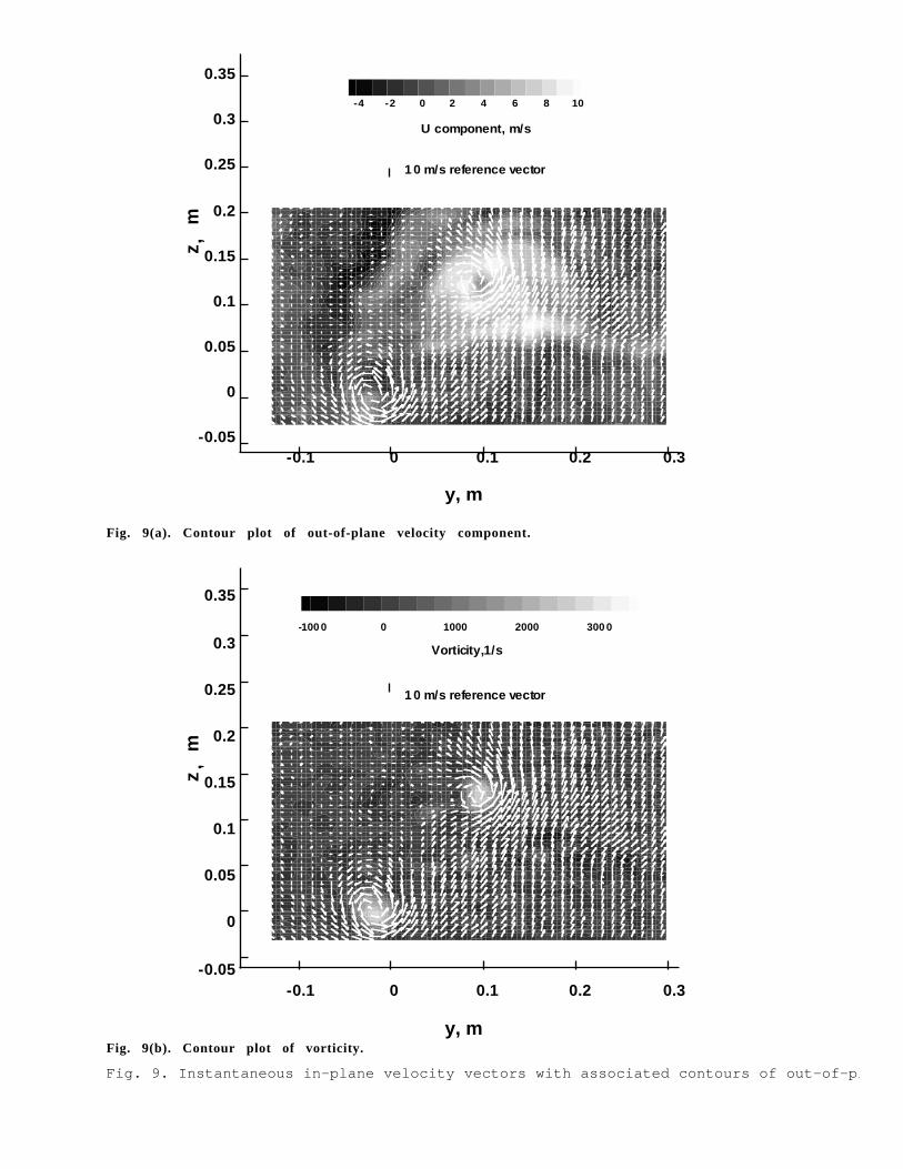
Instantaneous vs. Averaged Velocities: Fig.9 presents a single instantaneous realization of theflow field consistent with the image area shown inFig. 5. Fig. 9(a) shows in-plane velocities as vectorswith associated contours of out-of-plane velocities,where positive x is toward the reader. For clarity, thefigures show only one-fourth of the total calculatedvectors. Fig. 9(b) shows the same in-plane vectorfield with the associated contours of out-of-planevorticity. Two vortices are clearly definable in theflow field. The vortex in the lower left cornercorresponds to a wake age of 30 deg. The vortex inthe upper right corner corresponds to a wake age of210 deg. The horizontal streak in the center of Fig.9(a) represents the velocity defect associated with theblade wake.

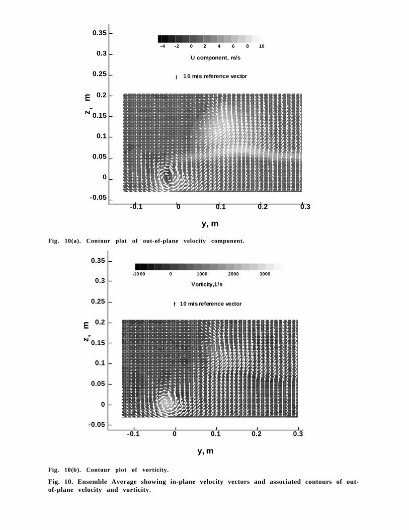
Fig. 10 presents the results of a simple averageof the data from the same test conditions of Fig. 9. Inthe course of processing, 14 vector fields wereeliminated due to recording errors or poor seeding.The simple average was performed with the remaining486 instantaneous vector fields, ignoring any effectsof vortex wander. Comparing the instantaneous flowfield in Fig. 9 with the mean flow field of Fig. 10several features are evident. First, the simple averagecomputes out-of-plane velocities and vorticity that aremuch lower than their instantaneous counterparts.Second, the trailed blade wake is still visible in Fig.10(a) but the average velocity defect in the blade wakeis considerably smaller than shown in Fig. 9(a).These differences can be attributed to vortex wander,as will be demonstrated in the following sections.

Vortex Wander Effects: Fig. 11 illustrates theamplitude of vortex wander observed at 30 deg. and210 deg. wake ages. The vortex centers, defined as thelocation of maximum instantaneous vorticity, wereplotted for each instantaneous field. Note the increasein amplitude of wander with increased wake age. Fig.12 shows histograms of vortex location for wake age210 deg.

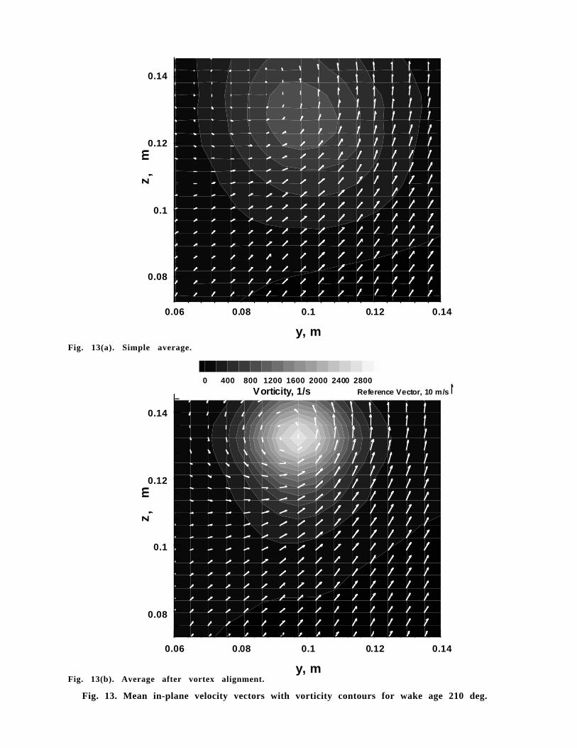
To further demonstrate the effects of vortexwander, Fig. 13 presents mean in-plane velocityvectors and contours of out-of-plane vorticity usingtwo different averaging techniques. These figuresshow all the vectors calculated in this region of the

flow field. The vortex wake age of 210 deg. waschosen to emphasize the effects of wander. Fig. 13(a),an expanded view taken directly from Fig. 10(b),shows the simple ensemble average. Fig. 13(b)shows the result of aligning vortex centers prior toaveraging. As expected, the simple average hasreduced the peak vorticity of the vortex core andredistributed it over a larger area in the flow field.Fig. 13(a) corresponds to the flow field that would bemeasured by point-sampling techniques such as LDV,hot-wire anemometry and pressure probemeasurements. Unlike PIV, these techniques have nomeans for correcting for vortex wander.

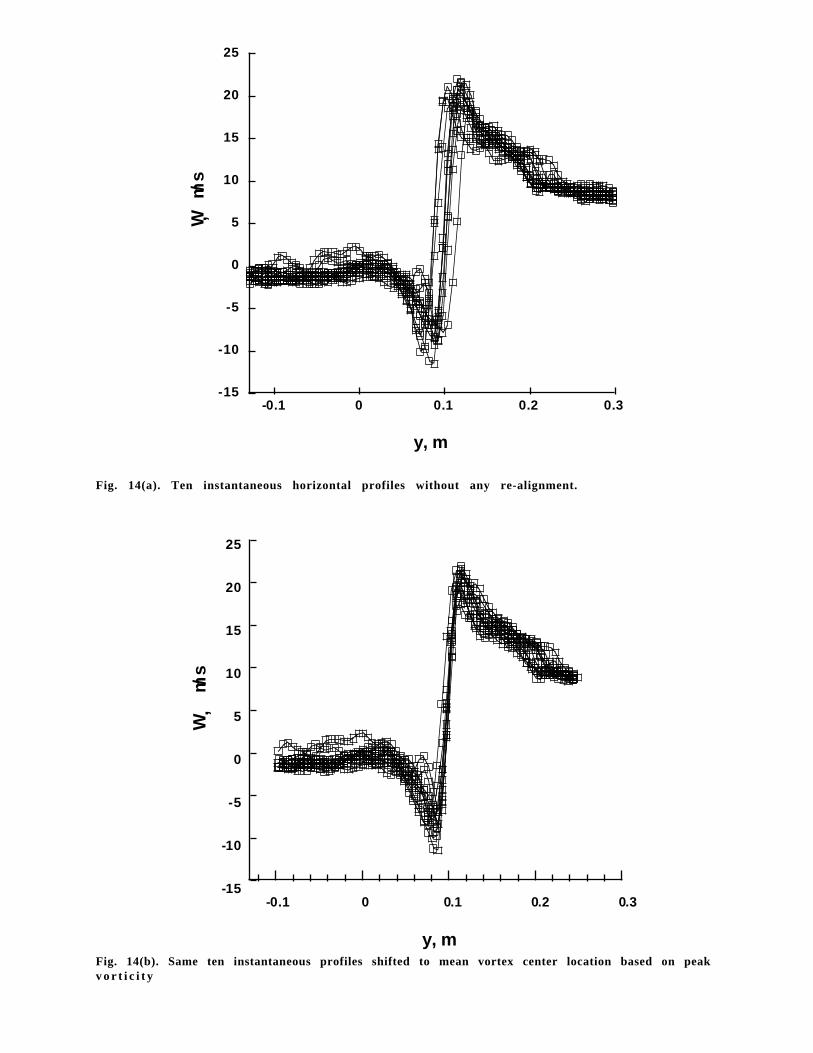
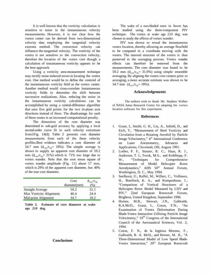
Vortex Core Measurements: The averagehorizontal vortex core diameter for the 210 deg. wakeage is calculated from instantaneous W componentprofiles of each vortex. The core diameter isdetermined by measuring the distance between thevelocity extrema of the profile. The profiles weredrawn horizontally through the vortex center locationsdetermined in the previous section. The averagemeasurement improves if the profiles undergo analignment procedure. Three methods for averaging arepresented. The first method takes a simple average ofthe velocity values at each line interval. Thiscorresponds to a point-wise measurement technique.The second method aligns the profiles using themaximum vorticity locations determined earlier. Thethird method aligns the midpoints of the velocityextrema for each profile.

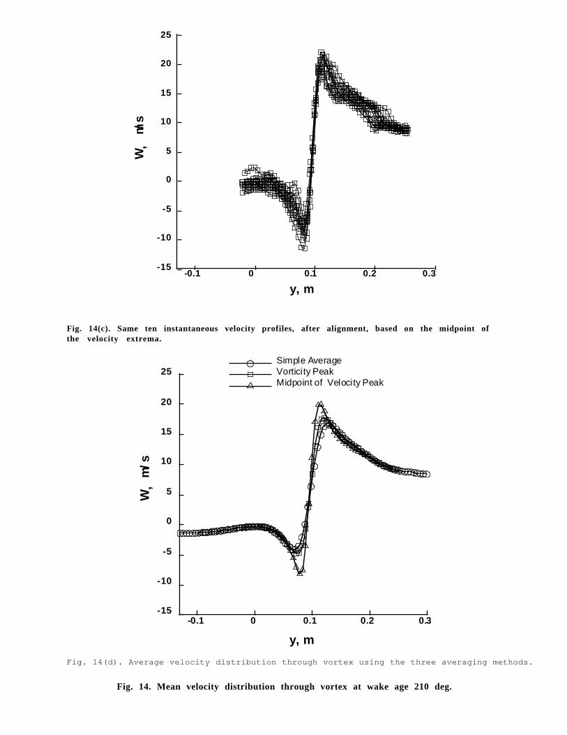
Fig. 14(a) shows several instantaneous profileswithout any attempt to align them horizontally. Onlyten are presented here for clarity. Fig. 14(b) shows thesame ten velocity profiles aligned according to the y-value of the maximum vorticity location. Fig. 14(c)shows the same ten profiles aligned using the centerlocations determined from the midpoint of thevelocity extrema of each instantaneous profile. Fig.14(d) shows the result of averaging all 486 profilesusing the three alignment methods. It is apparentfrom Fig. 14(d) that identification of the vortex centerwith the instantaneous peak vorticity is lesssuccessful than using the midpoint of the velocityextrema.

y, m

z ,m

-0.1 0 0.1 0.2 0.3-0.05

0

0.05

0.1

0.15

0.2

0.25

0.3

0.35

-4 -2 0 2 4 6 8 10

U component, m/s

1 0 m/s reference vector

Fig. 9(a). Contour plot of out-of-plane velocity component.

y, m

z,

m

-0.1 0 0.1 0.2 0.3-0.05

0

0.05

0.1

0.15

0.2

0.25

0.3

0.35

-100 0 0 1000 2000 300 0

Vorticity,1/s

1 0 m/s reference vector

Fig. 9(b). Contour plot of vorticity.

Fig. 9. Instantaneous in-plane velocity vectors with associated contours of out-of-pl

y, m

z ,m

-0.1 0 0.1 0.2 0.3-0.05

0

0.05

0.1

0.15

0.2

0.25

0.3

0.35

-4 -2 0 2 4 6 8 10

U component, m/s

1 0 m/s reference vector

Fig. 10(a). Contour plot of out-of-plane velocity component.

y, m

z ,m

-0.1 0 0.1 0.2 0.3-0.05

0

0.05

0.1

0.15

0.2

0.25

0.3

0.35

-10 00 0 1000 2000 3000

Vorticity,1/s

10 m/s reference vector

Fig. 10(b). Contour plot of vorticity.

Fig. 10. Ensemble Average showing in-plane velocity vectors and associated contours of out-of-plane velocity and vorticity.

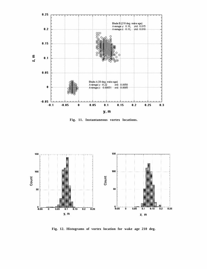
Fig. 11. Instantaneous vortex locations.

Fig. 12. Histograms of vortex location for wake age 210 deg.

y, m

z,

m

0.06 0.08 0.1 0.12 0.14

0.08

0.1

0.12

0.14

Fig. 13(a). Simple average.

y, m

z,

m

0.06 0.08 0.1 0.12 0.14

0.08

0.1

0.12

0.14

0 400 800 1200 1600 2000 2400 2800Vorticity, 1/s Reference Vector, 10 m/s

Fig. 13(b). Average after vortex alignment.

Fig. 13. Mean in-plane velocity vectors with vorticity contours for wake age 210 deg.

y, m

W ,m/

s

-0.1 0 0.1 0.2 0.3-15

-10

-5

0

5

10

15

20

25

Fig. 14(a). Ten instantaneous horizontal profiles without any re-alignment.

y, m

W,

m/s

-0.1 0 0.1 0.2 0.3-15

-10

-5

0

5

10

15

20

25

Fig. 14(b). Same ten instantaneous profiles shifted to mean vortex center location based on peakv o r t i c i t y

y, m

W,

m/s

-0.1 0 0.1 0.2 0.3-15

-10

-5

0

5

10

15

20

25

Fig. 14(c). Same ten instantaneous velocity profiles, after alignment, based on the midpoint ofthe velocity extrema.

y, m

W,

m/s

-0.1 0 0.1 0.2 0.3-15

-10

-5

0

5

10

15

20

25Simple AverageVorticity PeakMidpoint of Velocity Peak

Fig. 14(d). Average velocity distribution through vortex using the three averaging methods.

Fig. 14. Mean velocity distribution through vortex at wake age 210 deg.

It is well known that the vorticity calculation issensitive to noise in the instantaneous velocitymeasurements. However, it is not clear how thevortex center can be derived from two-dimensionalvelocity data employing the tangential velocityextrema method. The convection velocity caninfluence the tangential velocity. The vorticity of thevortex is not sensitive to the convection velocity,therefore the location of the vortex core though acalculation of instantaneous vorticity appears to bethe best approach.

Using a vorticity area-measurement techniquemay rectify noise-induced errors in locating the vortexcore. One method would be to define the centroid ofthe instantaneous vorticity field as the vortex center.Another method would cross-correlate instantaneousvorticity fields to determine the shift betweensuccessive realizations. Also, reducing the noise inthe instantaneous vorticity calculations can beaccomplished by using a central-difference algorithmthat uses five grid points for the two in-plane axisdirections instead of three. The disadvantage for eachof these routes is an increased computational penalty.

The dimension of the core diameter wasdetermined to sub-grid accuracy by applying a localsecond-order curve fit to each velocity extremumfrom1Fig. 14(d). Table 2 presents core diametermeasurements from each of the three velocityprofiles.Best evidence indicates a core diameter of34.7 mm (dcore/ctip= 18%). The simple average isshown to supply an apparent core diameter of 59.2mm (dcore/ctip= 31%) which is 71% too large due tovortex wander. Note that the root mean square ofvortex wander amplitude (Fig. 11) about 17 mm,which is 29% of the apparent core diameter, but 49%of the true core diameter.

Corediameter(mm)

dcore/ctip

(%)Straight Average 59.2 31.1Max Vorticity Ali gnment 46.4 24.4Mid-point Alignment 34.7 18.2

Table 2. Estimate of core diameter at wakeage 210 deg.

Conclusions

The wake of a two-bladed rotor in hover hasbeen studied using the three-component PIVtechnique. The vortex at wake age 210 deg. waschosen to study the effects of vortex wander.

PIV was shown to reveal the instantaneousvortex location, thereby allowing an average flowfieldto be computed in a coordinate moving with thevortex. The internal structure of the vortex is thuspreserved in the averaging process. Vortex wandereffects can therefore be removed from themeasurements. The core diameter was found to be59.2 mm (dcore/ctip= 31.0%) using simple ensembleaveraging. By aligning the vortex core centers prior toaveraging, a more accurate estimate was shown to be34.7 mm (dcore/ctip= 18%).

Acknowledgements

The authors wish to thank Mr. Stephen Walkerof NASA Ames Research Center for adapting his vortexlocation software for this experiment.

References

1. Grant, I., Smith, G. H., Liu, A., Infield, D., andEich, T., “Measurement of Shed Vorticity andCirculation from a Rotating Aerofoil by ParticleImage Velocimetry,” 4th International Conferenceon Laser Anemometry, Advances andApplications, Cleveland, OH, August 1991.

2. Lorber, P. F., Stauter, R. C., Haas, R. J.,Anderson, T. J., Torok, M.S., and Kohlhepp, F.W., “Techniques for ComprehensiveMeasurement of Model Helicopter RotorAerodynamics,” AHS 50th Annual Forum,Washington, D. C., May 1994.

3. Seelhorst, U., Raffel, M., Willert, C., Vollmers,H., Butefisch, K. A., and Kompenhans, J.,“Comparison of Vortical Structures of aHelicopter Rotor Model Measured by LDV andPIV,” 22nd European Rotorcraft Forum,Brighton, United Kingdom, September 1996.

4. Horner, M.B., Stewart, J.N., Galbraith,R.A.McD., Grant, I., Coton, F.N., “AnExamination of Vortex Deformation DuringBlade-Vortex Interaction Utilizing Particle ImageVelocimetry,” 19th Congress of the InternationalCouncil of the Aeronautical Sciences, Vol. 2,1994.

5. Coton, F. N., de la Inglesia Moreno, F.,Galbraith, R. A. McD., and Horner, M. B., “AThree-Dimensional Model of Low Speed Blade-Vortex Interaction,” 20th European Rotorcraft

Forum, Amsterdam, The Netherlands, October1994.

6. Saripalli, K.R., “Application of Particle ImagingVelocimetry Techniques to Helicopter RotorFlowfields at McDonnell Douglas Aerospace,”33rd AIAA Aerospace Sciences Meeting andExhibit, Reno, January 1995.

7. Murashige, A., Tsuchihashi, A., Tsujiuchi, T.,Yamakawa, E., “Blade-Tip Vortex Measurementby PIV,” 23rd European Rotorcraft Forum,Dresden, Germany, September 1997.

8. Willert, C., Raffel, M., and Kompenhans, J.,“Recent Applications of Particle ImageVelocimetry in Large-Scale Industrial WindTunnels,” International Congress onInstrumentation in Aerospace SimulationFacilities, Pacific Grove, CA, September-October 1997 (IEEE Publication 97CH36121).

9. Raffel, M., Willert, C., Kompenhans, J.,Ehrenfried, K., Lehmann, G., and Pengel, K.,“Feasibility and Capabilities of Particle ImageVelocimetry (PIV) for Large Scale Model RotorTesting,” AHS International Meeting onAdvanced Rotorcraft Technology and DisasterRelief, Gifu, Japan, April 1998.

10. Murashige, A., Kobiki, N., Tsuchihashi, A.,Nakamura, H., Inagaki, K., Yamakawa, E.,“ATIC Aeroacoustic Model Rotor Test at DNW,”AHS International Meeting on AdvancedRotorcraft Technology and Disaster Relief, Gifu,Japan, April 1998.

11. Yamauchi, G. K., Burley, C. L., Mercker, E.,Pengel, K., and JanakiRam, R., “FlowMeasurements of an Isolated Model Tilt Rotor,”AHS 55th Annual Forum, Montreal, Canada,May 1999.

12. Raffel, M., Dewhirst, T., Bretthauer, B., andVollmers, H., “Advanced Flow Velocity FieldMetrology and their Application to HelicopterAerodynamics,” 24th European Rotorcraft Forum,Marseilles, France, September 1998.

13. McAlister, K. W., Schuler, C. A., Branum, L.,and Wu, J. C., “3-D Wake Measurements Near aHovering Rotor for Determining Profile andInduced Drag,” NASA Technical Paper 3577,ATCOM Technical Report 95-A-006, August1995.

14. Lourenco, L. M., “Particle Image Velocimetry,”VKI Lecture Series, Particle Image Velocimetry,1996-06.

15. Arroyo, M. P. and Greated, C. A., “StereoscopicParticle Image Velocimetry,” MeasurementScience and Technology, 2, 1991.

16. Prassad, A. K. and Jensen, K., “ScheimpflugStereocamera for Particle Image Velocimetry inLiquid Flows,” Applied Optics, 34:7092-9,1995.

17. Raffel, M., Willert, C., and Kompenhans, J.,Particle Image Velocimetry, Springer-Verlag,1998.

18. Melling, A., “Tracer Particles and Seeding forParticle Image Velocimetry,” Measurement andScience Technology, Vol. 8, 1997.

19. Westerweel, J. “Theoretical Analysis of theMeasurement Precision and Reliability in PIV”,Proceedings of the Third International Workshopon PIV’99, 1999.

20. Lourenco, L., “Mesh-Free Second-Order AccurateAlgorithm for PIV Processing,” proceedings ofVSJ-SPIE98, Paper AB079, Yokohama, Japan,December 1998.