Application of the SWAT Model for Evaluating Discharge and

*Corresponding author’s e-mail: [email protected]

ASM Sc. J., 14, 2021

https://doi.org/10.32802/asmscj.2020.574

Application of the SWAT Model for Evaluating Discharge and Sediment Yield in the Huay Luang

Catchment, Northeast of Thailand

Haris Prasanchum1∗, Sasithum Phisnok1 and Sanhawit Thinubol2

1Faculty of Engineering, Rajamangala University of Technolgy Isan, Khon Kaen Campus, Khon Kaen, 40000, Thailand

2Regional Irrigation Office 5, Royal Irrigation Department, Udon Thani, 41000, Thailand

The climate change and insufficient data of the discharge and sediment yield in the catchment

system are the main cause of the conflict amongst the consumers. The application of a semi-

distributed hydrologic model and geographic information system can be a solution to this conflict.

This study implemented the SWAT model to estimate the discharge and sediment yield in the Huay

Luang Catchment, Northeast of Thailand. The accuracy of the model was affirmed and compared

with the data from the Kh103 observed station during 2008–2016 via SWAT-CUP. The study

outcome suggested that the SWAT model provided favourable results compared to the observed data

where R2, NSE, and PBIAS of the discharge were 0.79, 0.77, and -18.1% respectively and those of the

sediment yield were 0.68, 0.65, and -22.7% respectively. Additionally, the quantitative analysis on

22 sub-catchments as the spatial map derived from the Watershed Delineation indicated that both

discharge and sediment yield during 2008–2011 were higher than the regular values by 35.9% and

109.6% consecutively, whereas during 2012–2015 were lower than the regulars by 22.4% and 45.4%.

In the raining season, more than 50% of the sub-catchments demonstrated 9–20 cubic meter per

second of the discharge and 1,000–5,000 tons of the sediment yield, while during the drought

season, both volumes in most of the catchments indicated less than 6 cubic meter per second and

1,000 tons, respectively. These happened due to the changes of the rainfall each year. Hopefully, the

result and spatial information from this study could be a great contribution to the water resource

management and development in any catchment with insufficient data.

Keywords: discharge; sediment yield; Huay Luang Cathcment; SWAT; SWAT-CUP

I. INTRODUCTION

Nowadays, Thailand has launched a strategy to support the

general economic development such as agriculture, industry,

as well as the increasing number of the population; therefore,

there is higher demand for the land use for cultivating to

increase the product quantity and expanding the industrial

estate and residence area. This demand has yielded several

changes on the ground surface along with the rapidly growing

rate of the land use (Faksomboon & Thangtham, 2017), e.g.

the forest intrusion or changes of crop types (Roslee & Sharir,

2019). It is critically expected that these problems would

impact the hydrological system within the catchment areas;

for example, during the raining season, the discharge

following downwards the main stream and the sediment

yields washed out from the ground surface would be changed

so that the water quantity and quality was unfavourable for

water resource management in catchment areas (Arnold et.

al., 1998; Wuttichaikitcharoen & Babel, 2014; Ghani et al.,

2019) as well as decreasing the flow rate and increasing the

contamination of raw water. As a consequence, the

measurement and estimation of the discharge and sediment

yields within the streams could be the important data for

creating the water resource development plan. Still, there has

been an obstruction in collecting and filing the data from the

responsible organizations such as the Royal Irrigation

https://doi.org/10.32802/asmscj.2020.574

ASM Science Journal, Volume 14, 2021

2

Department or the Department of Water Resources due to the

problems in purchasing the advanced measurement tools or

the insufficient budget for maintenance. Accordingly, the

hydrological model could be another useful choice for the

data analysis on the discharge and sediment yield at the gauge

station with insufficient data or limited period of time for data

recording. This model is also time-saving and cost-saving for

the operation.

In the past, analysis of discharge and sediment yield in

catchment areas has been carried out using hydrologic

models, which are available in various forms, such as VIC,

TOPMODEL, HBV or MIKE-SHE, all of which are based on

water balance principles (Nourani et. al., 2011; Lasen et. al.,

2014; Oubeidillah et. al., 2014; Ali et al., 2018;). However,

each type of model will have different suitability depending

on the purpose to be analyzed. For example, VIC is suitable

for wetland areas and water management for agricultural

areas (Devi et al., 2015). MIKE-SHE has a huge demand for

importing physical data, which is a limitation for small river

catchments that lack data (Devi et al., 2015). While sediment

quantity studies using models such as GeoWEPP, SEDMODL

or RUSLE (Maalim et. al., 2013; Parsakhoo et al., 2014;

Ganasri & Ramesh, 2016) have a lot of basic operations or

require limited specific data such as satellite imagery.

Based on the literature review, each of the models has its

distinctive feature that differently matches with specific

objectives and usages and requires different types of input.

Each also has its own method for parameter adjustment to

provide the most favourable results. To do so, the model

needs a huge number of the input and highly delicate data so

it needs to work with a high-performing computer (Xia et al.,

2019) that match with the data calculation time.

Unfortunately, some catchment contains insufficient input

due to the lack of data, shortage of budget for digital file

creation, as well as incomplete primary data. Besides, some

forms of quantitative data from the model can be displayed as

either numbers or graphs, so it may need more specific

computer facilities to present the spatial data analysis. In case

of the insufficient input, an engineer or researcher may use a

hydrological model that can quickly calculate the data and

present different types of data from a single calculation. They

may apply it with GIS to obtain the hydroinformatics data

(Vojinovic & Abbott, 2017) for the stakeholders to effectively

solve the problematic water resources (Zardari et al., 2019).

As a result, a hydrological model with upgraded functions and

an ability to provide a favourable outcome for the catchment

with limitations or incomplete data is considered necessary.

Currently, the estimation of sediment and discharge in the

regional catchment using the Semi-Distributed Model (SDM)

is widely attractive because the results obtained from the

model can reflect the hydrological changes according to the

physical characteristics of the catchment area such as land

use, area slope and the local climate. The SWAT model is one

of the most widely semi-distributed hydrologic models in the

world (Cai et al., 2012), which has been applied for the study,

analysis, and evaluation of sediment and discharge problems

in the catchment, such as predict the sediment yield and in

small catchments that are affected by land use changes due to

increased population and construction demand (Cai et. al.,

2012; Huang & Lo, 2015; Zuo et al., 2016), estimation of

sedimentation from surface erosion (Son et al., 2015; Vidula

& Sushma, 2017), simulated discharge in the case of

catchments lacking gauge stations and spatial data (Mango et

al., 2011).

At this point, Huay Luang is a sub-catchment of Khong

Catchment in the northeast of Thailand where the discharge

coming along with the sediment yield has been a critical

problem that negatively affects the water resource

management. This varied the discharge efficiency and

sediment yield is expected to affect the carrying capacity of

the streams. Consequently, this research aimed to apply the

SWAT model for data evaluation on the discharge and

sediment yield in ungauged areas through classification as a

sub-catchment that covers the Huay Luang Catchment. It was

also expected that the methodology and outcome of this

research would be another approach to support the

responsible organization or person in deciding on the water

resource development planning in any target catchments

either at current state or in the future.

II. MATERIALS AND METHOD

A. Study Area

For the target area, in this study, the Huay Luang Catchment

is a sub-catchment of Khong Catchment in the northeast of

Thailand covering about 3,350 km2 of area where the Huay


3

Luang River flows from the southwest to the northeast as

presented in Figure 1(a). The annual average rainfall is 1,300

mm. The rainfall data was taken from 7 raingauge stations

separately located throughout the target catchment whereas

the climate data was obtained from the Udon Thani Station

located at the midst part of the catchment.

The observed discharge and sediment yield were taken from

the Kh103 Station located in the midst of the area were later

compared with the result of the model. The majority of the

population is engaged in agriculture using rainwater and

irrigation systems. The most commonly planted crops are rice,

cassava, sugarcane, and plantations. However, the problem of

intrusion in the upstream areas, the expansion of

communities near the water resource has expanded rapidly,

changes in cultivation patterns and global climate change in

the past 10 years are expected to directly affect the volume of

discharge and sediment yield in the Huay Luang Catchment.

B. SWAT Model

The SWAT (Soil and Water Assessment Tool) (Arnold et al.,

1998) is a hydrological model developed for evaluating

sediment change, discharge and water quality in rivers that

are affected by climate and land use changes in the past,

present and future forecasts (Mango et al., 2011). The model

can divide processing at multiple catchments at various levels,

such as creating sub-catchments in the main catchments,

including calculations that show daily and monthly results

and long period of time using water balance equations to be

considered based on variables from the hydrological process,

as illustrated in the Equation (1).

( )tt 0 day surf a seep qwi 1

SW SW R Q E W Q=

= + − − − − (1)

where SWt is final soil water content (mm), SW0 is initial soil

water content (mm), t is time (day), Rday is rainfall on Day i

(mm), Qsurf is surface water content on Day i (mm). Ea is

evapotranspiration content on Day i (mm), Wseep is

underground seepage content on Day i (mm), and Qgw is

underground water content flowing back to a stream on Day

i (mm) (Sajikumar & Remya, 2015).

Evaluation of sediment quantities using the SWAT model

used imported soil data in the model and determining the

physical properties of the soil as it affects the movement of

water and air, which is important for water circulation in each

hydrologic response unit. The important elements that affect

sedimentation in various streams include: 1) the volume and

the intensity of rainfall; 2) the characteristics of soil and rocks

in the catchment; 3) the characteristics of the soil cover, for

example, in case of the evergreen forest, there will be

sediment less than the deciduous forest; 4) the type of land

use, for example, if the area is always planted with ground

cover plants, erosion rates will be reduced; 5) topographical

conditions, such as if the slopes are very steep, the water will

flow more likely to cause erosion and; 6) other elements such

as size, shape and condition of use of the catchment. For the

equation used to assess sediment quantity in the SWAT

model, the model applied the Modified Universal Soil Loss

Equation (MUSLE) (Petsountang & Jirakajonhkool, 2012) as

exposed in Equation (2).

( )0.56

surf peakS 11.8 Q q K.LS.C.P= (2)

Where S is the total amount of sediment that flows out of the

cathcment (metric tons), Qsurf is the amount of water (m3),

qpeak is the maximum flow (m3 per second), K is the factor of

soil erosion stability is specific to each layer of the soil, LS is

the length and slope factor, C is the plant management factor,

P is the control factor for the erosion of soil, 11.8 and 0.56 are

the data constant values for each rainstorm applied to GIS.

C. Data Collection

The data collected and used with the SWAT model consisted

of the Digital Elevation Model (DEM) with a resolution of

30×30 m2, the soil types map, the land use map, the daily

climate data consist of; rainfall, maximum and minimum

temperatures, relative humidity, solar radiation, and wind

speed, as well as the discharge and sediment yield from the

Kh103 Station. Particularly, the land use data was surveyed

in 2015 classified into 9 groups in which most of the land was

used for rice field, sugarcane, cassava, generic agriculture,

and urbanization area (see Figure 1(b)).

The soil type data was assembled by the Land Development

Department of Thailand in 2015, accordance with the soil

classes of the SWAT model based on the Food and Agriculture

Organization (FAO, 2006) textural classes including 5 soil

groups: most of them were in Sandy loam, sandy loam clay

(SL, SCL) and Clay (C) in north part (see Figure 1(c)). All of

these data for input to the SWAT model and for the model


4

performance evaluation were presented clearly in Table 1.

Table 1. Spatial data and observed discharge data for the

SWAT model performance evaluation

Data types Period Scale Source

Spatial data (model input)

DEM 2015 30×30 m

LDD River map 2015

1:50,000 Soil types 2015

Land use 2015

Climate 2008−2016 Daily TMD

Observed sediment and discharge

(model performance assessment)

Kh103 2008−2016 Daily RID

Remarks;

LDD : Land Develop Department

TMD : Thai Meteorological Department

RID : Royal Irrigation Department

D. Sub-Catchment Modeling and HRUs Analysis

The study area, Huay Luang Catchment was defined from the

DEM input used for the evaluation on the physical use types

characteristics of the sub-catchment; meanwhile, the land

and the soil types were defined by inserting the land use map

and soil types map into the SWAT model so that they could

be linked with the data from the study area. The

determination of Hydrological Response Units (HRUs) (Cai

et. al., 2012; Noh et al., 2019) was the stage to define the

resolution of the catchment unit in which the sub-catchment

normally contains different HRUs, e.g. those that were

consistent with the types of land use and land cover, the soil

groups, the land slope, etc.

Regularly, these HRUs are diversified by each specific area

as well as by the hydrological conditions based on the

meteorological factors of each HRUs. Indeed, the HRUs

determination had further impact on the model accuracy

estimation during the sensitivity analysis of hydrological

parameters. In term of the climate input, there were 5 key

parameters including: 1) rainfall; 2) maximum and minimum

temperatures; 3) relative humidity; 4) wind speed; and 5)

solar radiation. These parameters were daily data that was

presented in Table 1 arranged in a favourable order for the

SWAT model.

(a) (b) (c)

Figure 1. Spatial data of the Huay Luang Catchment, (a) study area and DEM, (b) land use types map and (c) soil types map


5

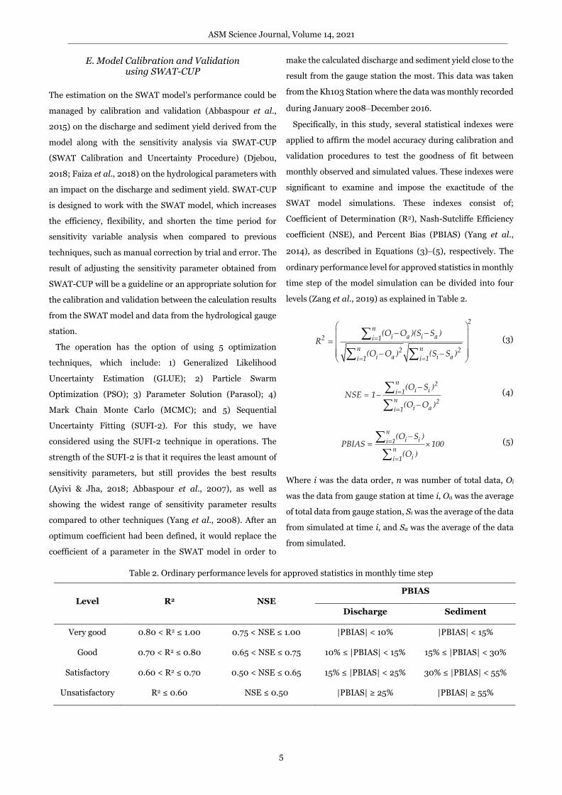
E. Model Calibration and Validation using SWAT-CUP

The estimation on the SWAT model’s performance could be

managed by calibration and validation (Abbaspour et al.,

2015) on the discharge and sediment yield derived from the

model along with the sensitivity analysis via SWAT-CUP

(SWAT Calibration and Uncertainty Procedure) (Djebou,

2018; Faiza et al., 2018) on the hydrological parameters with

an impact on the discharge and sediment yield. SWAT-CUP

is designed to work with the SWAT model, which increases

the efficiency, flexibility, and shorten the time period for

sensitivity variable analysis when compared to previous

techniques, such as manual correction by trial and error. The

result of adjusting the sensitivity parameter obtained from

SWAT-CUP will be a guideline or an appropriate solution for

the calibration and validation between the calculation results

from the SWAT model and data from the hydrological gauge

station.

The operation has the option of using 5 optimization

techniques, which include: 1) Generalized Likelihood

Uncertainty Estimation (GLUE); 2) Particle Swarm

Optimization (PSO); 3) Parameter Solution (Parasol); 4)

Mark Chain Monte Carlo (MCMC); and 5) Sequential

Uncertainty Fitting (SUFI-2). For this study, we have

considered using the SUFI-2 technique in operations. The

strength of the SUFI-2 is that it requires the least amount of

sensitivity parameters, but still provides the best results

(Ayivi & Jha, 2018; Abbaspour et al., 2007), as well as

showing the widest range of sensitivity parameter results

compared to other techniques (Yang et al., 2008). After an

optimum coefficient had been defined, it would replace the

coefficient of a parameter in the SWAT model in order to

make the calculated discharge and sediment yield close to the

result from the gauge station the most. This data was taken

from the Kh103 Station where the data was monthly recorded

during January 2008−December 2016.

Specifically, in this study, several statistical indexes were

applied to affirm the model accuracy during calibration and

validation procedures to test the goodness of fit between

monthly observed and simulated values. These indexes were

significant to examine and impose the exactitude of the

SWAT model simulations. These indexes consist of;

Coefficient of Determination (R2), Nash-Sutcliffe Efficiency

coefficient (NSE), and Percent Bias (PBIAS) (Yang et al.,

2014), as described in Equations (3)−(5), respectively. The

ordinary performance level for approved statistics in monthly

time step of the model simulation can be divided into four

levels (Zang et al., 2019) as explained in Table 2.

2n

i a i a2 i 1

n n2 2i a i ai 1 i 1

(O O )(S S )R

(O O ) (S S )

=

= =

− −

= − −

(3)

n 2i ii 1

n 2i ai 1

(O S )NSE 1

(O O )

=

=

−= −

−

(4)

ni ii 1

nii 1

(O S )PBIAS 100

(O )

=

=

−=

(5)

Where i was the data order, n was number of total data, Oi

was the data from gauge station at time i, Oa was the average

of total data from gauge station, Si was the average of the data

from simulated at time i, and Sa was the average of the data

from simulated.

Table 2. Ordinary performance levels for approved statistics in monthly time step

Level R2 NSE PBIAS

Discharge Sediment

Very good 0.80 < R2 ≤ 1.00 0.75 < NSE ≤ 1.00 |PBIAS| < 10% |PBIAS| < 15%

Good 0.70 < R2 ≤ 0.80 0.65 < NSE ≤ 0.75 10% ≤ |PBIAS| < 15% 15% ≤ |PBIAS| < 30%

Satisfactory 0.60 < R2 ≤ 0.70 0.50 < NSE ≤ 0.65 15% ≤ |PBIAS| < 25% 30% ≤ |PBIAS| < 55%

Unsatisfactory R2 ≤ 0.60 NSE ≤ 0.50 |PBIAS| ≥ 25% |PBIAS| ≥ 55%


6

III. RESULTS AND DISCUSSION

A. Sensitivity Parameter Analysis

The parameter sensitivity analysis was performed via SWAT-

CUP using SUFI-2 in which 500 calculation rounds were

defined, as 8 and 4 parameters affecting the discharge and

sediment yield were also prescribed respectively. The

optimum outcome making the calculated result mostly

similar to the discharge and sediment yield measured at the

gauge station were described in Table 3. In terms of using

SUFI-2 to analyze the order of sensitivity parameters, the

basic principle of analysis was based on t-stat and P-value.

When the results indicate the highest t-stat, the parameter

has the best relationship (when + and – were excluded),

whereas P-value shows the significance of sensitivity. If P-

value was close to zero, that parameter was most significant.

The result from t-stat and P-value impacted the discharge and

sediment yields based on the sensitivity order presented in

Table 3.

Both t-stat and P-value indicated that SOL_AWC and

USLE_P were mostly related to the model’s sensitivity

(Regular P-value <= 0.05). No.3–5 were the parameters

related with the groundwater including GW_REVAP,

GWQMN, and ALPHA_BF, and No.6–7 were the sediment-

related parameters including SPCON and SPEXP. The rest

were ESCO, the parameter related to ground-surface

infiltration, followed by No.9–10, the evaporation in shallow

aquifer and groundwater parameters including REVAPMN

and GW_DELAY. Finally, LAT_SED and CN2 are displayed

in the No.11 and 12 positions.

According to the parameter adjustment via SWAT-CUP, the

analysis on the sensitivity parameter between the discharge-

related and sediment yield-related parameters indicated that

the surface discharge (No.1: SOL_AWC) and the soil loss

(No.2: USLE_P) were amongst the top influential parameters

(Khalid, et al., 2016; Hosseini & Khaleghi, 2020) and this

implied that the surface discharge directly had a significant

relation with the sediment yield (Khelifa et al., 2017; Worku

et al., 2017) connected through the variables related to the

evaporation of the groundwater (No.3–5) and the sediment

in the rivers (No.6-7), respectively.

B. Model Calibration and Validation

The complete data of discharge and sediment yield from the

Kh103 Station between 2008−2016 is considered to be

compared with the calculation results from the SWAT model.

Due to the limitation of the data from the observed station is

only 9 years (sediment yield has only 8 years-no recorded in

2014), as well as the annual volume of discharge and

sediment yield that has changed to the extreme during the

considered period. Figure 2 shows the total annual volume

data of both variables (recorded from the observed station)

which indicates the year 2008−2011, and both variables have

normal-high volume (in 2011 Thailand has the Great Flood

event). On the contrary, between 2012−2016, both volumes

were lower than average. To make it reasonable to calibrate

between the model and the observed values, and to cover the

fluctuate situation was described earlier. The selection of the

calibration period is used during 2011−2016 (6 years) in order

to cover between high and low volume events. While the

validation will be between 2008−2010 (3 years) which covers

the near normal and high volume.

The calculated result from the SWAT model compared with

the data at the Kh103 Station recorded during 2008−2016

was shown in Table 4. The results of the model accuracy

evaluation of both discharge and sediment yield have

suggested that the overall values of R2 is within the criteria

"good" (0.79 and 0.68), NSE is "good" (0.77 and 0.65) and

PBIAS is "satisfactory" (discharge, -18.1%) and "good"

(sediment yield, -22.7%). For compatibility between the

model results and the actual observed values of discharge and

sediment yield at the Kh103 Station, the monthly hydrograph

is shown in Figure 3(a) and (b), respectively. The results

indicated that the SWAT model can be applied to assess

discharge and sediment yield for the Huay Luang Catchment

with acceptable accuracy.


7

Table 3. Calibrated sensitivities parameters and fitted values using SUFI-2 from SWAT-CUP

Rank Parameters Description Fitted

Value

Adjust

Range t-stat P value

1 V_SOL_AWC.sol Available water capacity of the

soil layer 0.595 0.0 – 1.0 2.71 0.00

2 V_USLE_P.mgt USLE equation support (P) 0.00125 -0.2 – 0.2 -2.02 0.05

3 V_GW_REVAP.gwt Groundwater "revap" coefficient 0.1325 0.02 – 0.2 -1.51 0.13

4 V_GWQMN.gwt

Treshold depth of water in the

shallow aquifer required for

return flow to occur

4,733.75 4,250 – 5,000 -1.15 0.25

5 V_ALPHA_BF.gwt Baseflow alpha factor 0.465 0.0 – 1.0 0.80 0.42

6 V_SPCON.bsn

Linear parameter for calculating

the maximum amount of

sediment that can be re-

entrained during channel

sediment routing

0.002228 0.0001 –

0.005 0.59 0.56

7 V_SPEXP.bsn

Exponent parameter for

calculating sediment

reentrained in channel sediment

routing

1.655 1.0 – 2.0 0.39 0.69

8 V_ESCO.hru Soil evaporation compensation

factor 0.115 0.0 – 1.0 0.37 0.70

9 V_REVAPMN.gwt

Threshold depth of water in the

shallow aquifer for "revap" to

occur

372.5 0.0 – 500.0 -0.30 0.76

10 V_GW_DELAY.gwt Groundwater delay 86.7 0.0 – 500.0 -0.26 0.79

11 V_LAT_SED.hru

Sediment concentration in

lateral flow and groundwater

flow

98.5 0.00 – 100.0 0.16 0.86

12 R_CN2.mgt SCS runoff curve number 0.142 -0.2 – 0.2 0.13 0.89

Figure 2. The total of annual volume of discharge and sediment yield during 2008−2016 from the Kh103 Station

0

5,000

10,000

15,000

20,000

25,000

30,000

35,000

40,000

0

20

40

60

80

100

120

140

160

180

2008 2009 2010 2011 2012 2013 2014 2015 2016

Se

dim

en

t y

ield

(T

on

s)

Dis

cha

rge

(C

MS

)

Time (Years)

Discharge

Maen discharge

Sediment yield

Mean Sediment yield


8

(a)

(b)

Figure 3. Comparison of observed and simulation of (a) discharge and (b) sediment yield at monthly time scale

Table 4. Model performance results

Range Assessment index

R2 NSE PBIAS

Discharge

Calibration (2011−2016) 0.81 0.79 -22.8%

Validation (2008−2010) 0.76 0.75 -13.1%

Overall (2008-2016) 0.79 0.77 -18.1%

Sediment yield

Calibration (2011−2016) 0.64 0.60 -34.6%

Validation (2008−2010) 0.73 0.72 -12.3%

Overall (2008-2016) 0.68 0.65 -22.7%

For the next step, the SWAT model that has been adjusted

for accuracy in this calculation will be considered to assess

the volume of discharge and sediment yield within the 22 sub-

catchments (divided by the watershed delineation process of

the SWAT model). This evaluation can be carried out in the

form of spatial maps, based on the range of colours and

quantities to indicate changes in the volume of discharge and

sediment yield of the sub-catchment areas and time series.

C. Spatial Distribution of Discharge and Sediment Yield in Sub-catchment Level

After the SWAT model had finished calibrating and validating

the discharge and sediment yield at the observed station and

gained the satisfactory results, both values from all 22 sub-

catchments after the watershed delineation were later

summarized to define the annual averages and the input data

for the ArcGIS that would be displayed as the spatial

distribution map covering the Huay Laung Catchment during

2008–2016 as well as the average during the dry season

(November–May) and the wet season (June–October).

Figure 4 and 5 show the annual averages of the discharge and

sediment yield found in those sub-catchments. In the figures

of each year, the monthly averages (bar graph) would be

compared with the regular values (the blue dash line

represented the discharge and the brown dash line

represented the sediment yield).

1. Discharge

Regarding the annual discharge average, Figure 4 noted that

during 2008–2011, the discharge was higher than the regular

value by 35.9%−109.6% (the discharge average in the Huay

Laung Catchment is approximately 81.4 CMS per year as

shown in Figure 2). Exactly, most of the discharge averages

from the sub-catchments in the northeast area and the north

could be 9−20 CMS since the monthly averages in the raining

season were higher than the regular value, especially in 2009

and 2011 so that there was the Great Flood in the northeast

and Thailand. On the contrary, during 2012−2015, it was

found that the annual discharge averages from all sub-

catchments were lower than the regular value by

22.4%−45.4%; this could be apparently observed in periods of

2012−2013 and 2015 where the discharge averages from

12−14 sub-catchments, mostly in the southern west, were only

0−3 CMS, and 6−10 sub-catchments in the northeast were 3−6

CMS. Notably, in 2016, the averages were slightly higher than

the regular value by 5.4% where the discharge averages were

merely 0−12 CMS. During the dry season from November to

May, the averages were lower than 6 CMS, whereas, in the wet

season from June to October, there was 10 sub-catchments

where the averages were 9−20 CMS. In this regard, the sub-

catchments with high averages were mostly found in the

northeast and the north areas since it was a lowland (most of

the land was used as the rice field) and the outlet of the Huay

Luang Catchment. Differently, the southern west was a steep

0

10

20

30

40

50

60

70

80

90

Jan-08 Jan-09 Jan-10 Jan-11 Jan-12 Jan-13 Jan-14 Jan-15 Jan-16

Dis

cha

rge

(C

MS

)

Times (Months/Years)

observedsimulated

CalibrationValidation

0

2,000

4,000

6,000

8,000

10,000

12,000

14,000

16,000

Jan-08 Jan-09 Jan-10 Jan-11 Jan-12 Jan-13 Jan-14 Jan-15 Jan-16

Se

dim

en

t lo

ad

(T

on

s)

Times (Months/Years)

observedsimulated

Validation Calibration

No

da

ta r

eco

rde

d


9

land covered with forest and widely used for growing

sugarcane (see Figure 1(a) and Figure 1(b)) so that the

discharge there have constantly been low (Sriworamas et al.,

2020) all year round.

2. Sediment Yield

Figure 5 presents the annual sediment yield averages in the

Huay Luang Catchment during 2018−2016 which was

16,817.8 tons per year when compared to the regular average

(see Figure 2); therefore, there were 4 periods from

2008−2011 when the sediment yield was 50% higher than the

regular average; this was consistent with the discharge

averages found in the same periods. The sub-catchments with

high averages were mostly situated in the north and the

northeast. Particularly in 2011 when the sediment yield

average was much higher than the regular value by 172.7%

(45,855 ton per year), it was found that 10 sub-catchments

bears 2,000−6,000 tons of sediment yield or over 50% of the

whole area and it was often found during the wet season

lasting to the dry season or from August to December and the

next January. Still, the sediment yield averages lower than

the regular value could be found in 2012 (-37.5%) and 2015

(-39.6%) where all the sediment yield averages in all sub-

catchments were lower than 1,000 tons. Additionally, the

optimum average was found in 2014 where it was higher than

the regular value by only 6.4%.

When considering the averages by seasons, the sediment

yield in the dry season did not exceed 1,000 tons in every sub-

catchment, whereas the averages in the wet season were from

1,000−5,000 tons spreading through 13 sub-catchments.

However, the sediment yield with average of 4,000−5,000

tons were typically found at the northern outlet in main

catchment, followed by the physical attribute of the area,

where the sediment yield was naturally assembled at

catchment outlet. On the other hands, in the upstream with

the steep area, the sediment yield would be commonly low.

Meanwhile, the moderate sediment yield average could be

found in the midst of the catchment. In case of the sub-

catchments with high sediment yield averages, either the

measurements or extra activities should be managed for

surface water improvement, e.g. soil surface preservation,

forest expansion, suitable crop selection, increasing dredging

budget, etc.

D. Analysis of Discharge and Sediment Yield within Sub-catchment Area

Based on the findings from the previous section, the wet

season is a period with the highest discharge and sediment

yield, which is consistent with the results of studies in many

areas (Zhang et. al., 2016; Azari et al., 2019) that might have

some impact on the water resource management (particularly

for the sediment yield management); therefore, in this study,

magnitude of the discharge and sediment yield that has an

impact on the sub-catchment area (Djebou, 2018) is

determined by referring to the average in the wet season from

2008−2016. The results of volume comparison in percentages

are shown in Table 6 and Figure 6. The compared results in

Figure 6(a) indicated that the annual discharge average

during the wet season was 166.5 CMS and 38.4% of the sub-

catchments (No. 1, 2, 5, 7, 8, and 9) contained 12−20 CMS so

that the total average was 77.2%. This mostly happened in the

north and the northeast. Meanwhile, 39.3% of the sub-

catchments mostly covering the southern west and some

parts of the north showed the average lower than 3 CMS that

could roughly produce 4.7% of the discharge, whereas

approximately 22.3% of the sub-catchments mostly in the

central part of the area contained a moderate value of 6−12

CMS. Hence, the total average was 18.1% of the total

discharge in the wet season.

As the annual sediment yield average during the same

period was 49,768.9 tons. In this regard, the comparison

between the area and the average was illustrated in Figure

6(b). It indicated that the majority of 49.3% of the area

showed the sediment yield averages from 2,000−4,000 tons

or 64.1% of the total. The spatial distribution covered the

central part spreading toward the upper and lower parts of

the catchment. Besides, the minimum sediment yield of

0−2,000 tons was found in 42.1% of the area and the total

yield was 18.6%. Most of this case was basically found in the

upstream in the south and the downstream in the north,

meanwhile, the maximum of 4,000−5,000 tons were found in

only 8.6% of the area, but it somehow produced 17.4% of the

total sediment yield average which could be evidently seen at

the northern outlet (Sub-catchment No.1 and 2).


10

2008

2009

2010

2011

2012

2013

2014

2015

2016

Dry season

Wet season

Figure 4. Magnitude of annual discharge across the sub-catchments delineated within the Huay Luang Catchment


11

2008

2009

2010

2011

2012

2013

2014

2015

2016

Dry season

Wet season

Figure 5. Magnitude of annual sedient yield across the sub-basins delineated within the Huay Luang Catchment


12

Table 6. Evaluation of discharge and sediment yield of the sub-catchment attended in the catchment area during the wet

season

Range of

volume

Number of Sub-

catchments

Corresponding area Total of volume

Area Percentage

of area

Volume

per year

Percentage

of volume

Discharge (CMS) (km2) (%) (CMS) (%)

0 - 3 11 1,315.7 39.3 7.9 4.7

3 - 6 - - - - -

6 - 9 1 370.3 11.0 7.7 4.6

9 - 12 2 378.2 11.3 22.4 13.4

12 - 15 2 212.4 6.3 29.5 17.7

15 - 20 6 1,074.8 32.1 99.1 59.5

Total 22 3,351.3 100.0 166.5 100.0

Sediment yield (Tons) (km2) (%) (Tons) (%)

0 – 1,000 6 781.0 2,809.4 23.3 5.6

1,000 – 2,000 4 630.4 6,424.0 18.8 12.9

2,000 – 3,000 5 915.8 13,838.0 27.3 27.8

3,000 – 4,000 5 736.0 18,043.5 22.0 36.3

4,000 – 5,000 2 288.1 8,654.0 8.6 17.4

5,000 – 6,000 - - - - -

Total 22 3,351.3 49,768.9 100.0 100.0

(a)

(b)

Figure 6. Comparison of percentage between sub-catchment areas with (a) discharge and (b) sediment yield divided by

quantity range in the wet season

0

10

20

30

40

50

60

0-3 3-6 6-9 9-12 12-15 15-20

Perc

en

tag

e (

%)

Range of average annual discharge (CMS/year)

Percentage of total catchment area

Percentage of total discharge

0

10

20

30

40

50

60

0-1,000 1,000-2,000 2,000-3,000 3,000-4,000 4,000-5,000 5,000-6,000

Perc

en

tag

e (

%)

Range of average annual sediment yield (Tons/year)

Percentage of total catchment area

Percentage of total sediment yield


13

By mainly analyzing the relationship and similarity

between the area and both averages (discharge and sediment

yield) found in the wet season, any sub-catchments all

together producing the closet value or more than 50% of the

total area could increase over 80% of the total discharge so

the result from this study revealed that 49.7% of the sub-

catchments gave 90.6% of the total annual discharge average;

meanwhile, 57.9% of the total area could produce 81.5% of

the total sediment yield. Both values demonstrated the

spatial distribution in which the sub-catchments with

moderate and high averages were mainly located in the

central part and the north of the main catchment. This

assessment firmly indicated that more than 50% of the sub-

catchments within the Huay Luang Catchment had its

potential to produce more than 90% of the discharge. Still, it

also caused more than 80% of sediment yields. Accordingly,

the discharge and sediment yield at the downstream should

be managed systematically.

IV. CONCLUSION

When applying the SWAT model with spatial data for the

discharge and sediment yield estimation in the Huay Laung

Catchment, the data from the Kh103 Station during

2008−2016 was calibrated and validated, and 12 sensitivity

parameters with an impact on the discharge and sediment

yields were analyzed by SWAT-CUP with SUFI-2

optimization technique to define the optimal sensitivity

parameters for the model modification and to gain similar

result as the real values. During the calibration and validation

periods, the monthly of R2 and NSE are respectively 0.79 and

0.77 which were “good” for the discharge and 0.68 and 065

which were “satisfactory” for the sediment yields. In term of

PBIAS, both were proved to be lower than the observed, so

they were negative. Namely, the discharge was -18.1% and the

sediment yield was -22.7% which were “good” and

“satisfactory” consecutively.

The highlight of the SWAT model used in this study was a

watershed delineation process that classifies the Huay Luang

Catchment into several sub-catchments and the 22 sub-

catchments were studied. At this point, the difference in the

discharge averages in those sub-catchments were in a range

from 0.05−18.1 CMS per year while the sediment yield

averages could be 0−4,136.8 tons per year. Besides, after

considering the area size in the wet season with maximum

discharge and sediment yield, more than 50% of the sub-

catchments area could produce 90% of the discharge and

82% of sediment yields, respectively. Notably, these high

averages were mostly found in the northeast and the north

since it was the catchment outlet. This finding was very

contributive to this study since it helped simulate the

discharge and sediment yield averages and presented them as

the spatial distribution processed through the Geographic

Information System (GIS) in the ArcGIS. Hence, it was

possible to observe a sensitive area without observed gauge

station and with unknown data that may cause a problem for

the responsible organization or stakeholders in managing the

water resource around the main catchment.

In summary, the research methodology and outcomes from

the discharge and sediment yield evaluation using the SWAT

model was expected to be greatly contributive to the making

of future water resource management plan in both qualitative

and quantitative approaches such as the assessment on the

flood and drought risk, improvement of water quality for

consumption, the environmental conservation for the Huay

Luang Catchment or other regional catchments with similar

physical features, as well as any catchments with insufficient

measuring instrument and observed station for better

performance through the sustainable collaboration amongst

all related sector.

V. ACKNOWLEDGEMENT

The researcher would like to thank the Civil Engineering

Department, Faculty of Engineering, Rajamangala University

of Technology Isan (RMUTI), Khon Kaen Campus, for the

research instruments and laboratory support for this

research. Above all, the researcher also owed a debt of

gratitude to the Land Development Department, the Thai

Meteorological Department and the Regional Irrigation

Office 6 (Khon Kaen), Royal Irrigation Department of

Thailand, for the useful data for this research.


14

VI. REFERENCES

Abbaspour, KC, Rouholahnejad, E, Vaghefi, S, Srinivasan, R,

Yang, H & Klove, B 2015, ‘A Continental-scale hydrology

and water quality model for Europe: calibration and

uncertainty of a high-resolution large-scale SWAT model’,

Journal of Hydrology, vol. 524, pp. 733–752.

Abbaspour, KC, Yang, J, Maximov, I, Siber, R, Bognerb, K,

Mieleitner, J, Zobrist, J & Srinivasan, R 2007, ‘Modelling

hydrology and water quality in the pre-alpine/alpine Thur

watershed using SWAT’, Journal of Hydrology, vol. 333, pp.

413-430. doi:10.1007-/s40710-015-0064-8.

Ali, AF, Cun-de, X, Xiao-peng, Z, Adnan, M, Iqbal, M & Khan,

G 2018, ‘Projection of future streamflow of the Hunza River

Catchment, Karakoram Range (Pakistan) using HBV

hydrological model’, Journal of Mountain Science, vol. 15,

no. 10, pp. 2218–2235.

Arnold, AG, Srinivasan, R, Muttiah, RS & Williams, JR 1998,

‘Large area hydrological modeling and assessment part I:

model development’, Journal of American Water Resource

Association, vol. 34, no. 1, pp. 73–89.

Ayivi, F & Jha, MK 2018, ‘Estimation of water balance and

water yield in the Reedy Fork-Buffalo Creek Watershed in

North Carolina using SWAT’, International Soil and Water

Conservation Research, vol. 6, pp. 203–213.

Azari, M, Moradi, HR, Saghafian, B & Faramarzi, M 2016,

‘Climate change impacts on streamflow and sediment yield

in the North of Iran’, Hydrological Sciences Journal, vol. 61,

no. 1, pp. 123–133.

Cai, T, Li, Q, Yu, M, Lu, G, Cheng, L & Wei, X 2012,

‘Investigation into the impacts of land-use change on

sediment yield characteristics in the upper Huaihe River

catchment, China’, Physics and Chemistry of the Earth, vol.

53-54, pp. 1–9.

Dagbegnon, C & Sohoulande, D 2018, ‘Assessment of

sediment inflow to a reservoir using the SWAT model under

undammed condition: a case study for the Somerville

Reservoir, Texas, USA’, Journal of International Soil and

Water Conservation Research, vol. 6, pp. 222–229.

Devi, GK, Ganasri, BP & Dwarakish, GS 2015, ‘A review on

hydrological models’, Aquatic Procedia, vol. 4, pp. 1001–

1007.

Djebou, DCS 2018, ‘Assessment of sediment inflow to a

reservoir using the SWAT model under undammed

condition: a case study for the Somerville Reservoir, Texas,

USA’, Journal of International Soil and Water Conservation

Research, vol. 6, no. 3, pp. 222–229.

Faiza, H, Mohamed, M, Gil, M, Salaheddine, A & Abdelkader,

K 2018, ‘Modeling of discharge and sediment transport

through SWAT model in the Catchment of Harraza

(Northwest of Algeria)’, Journal of Water Science, vol. 32,

pp. 79–88.

Faksomboon, B & Thangtham, N 2017, ‘Application of SWAT

model for studying land use changes on suspended

sediment in Upper Tha Chin watershed’, Journal of SWU

Science, vol. 33, pp. 124–139.

Food and Agriculture Organization of the United Nations

(eds) 2006, Guidelines for soil description, 4th edn,

Publishing Management Service Information Division,

FAO, Rome, Italy.

Ganasri, BP & Ramesh, H 2016, ‘Assessment of soil erosion

by RUSLE model using remote sensing and GIS – a case

study of Nethrathi Catchment’, Geoscience Frontiers, vol. 7,

no. 6, 953-961.7(special issue), pp. 72–84.

Ghani, NAAA, Tholibon, DA & Ariffin, J 2019, ‘Robustness

analysis of model parameters for sediment transport

equation development’, ASM Science Journal, vol. 12. doi:

10.32802/asmscj.2019.268.

Hosseini, SH & Khaleghi, MR 2020, ‘Application of SWAT

and SWAT-CUP software in simulation and analysis of

sediment uncertainty in semi-arid watersheds (case study:

the Zoshk-Abardeh watershed)’, Modeling Earth System

and Environment. doi: 10.1007/s40808-020-00846-2.

Huang, TCC & Lo, KFA 2015, ‘Effects of land use change on

sediment and water yields in Yang Ming Shan National

Park, Taiwan’, Environments, vol. 2, pp. 32–42.

doi:10.3390/environments2010032.

Khalid, K, Ali, MF, Rahman, NFA, Mispan, MR, Haron, SH,

Othman, Z & Bachok, MF 2016, ‘Sensitivity analysis in

watershed model using SUFI-2 algorithm’, Procedia

Engineering, vol. 162, pp. 441-447.

Khelifa, WB, Hermassi, T, Strohmeier, S, Zucca, C, Ziadat, F,

Boufaroua, M & Habaieb, H 2017, ‘Parameterization of the

effect of bench terraces on runoff and sediment yield by

SWAT dodeling in a small semi-arid watershed in Northern

Tunisia’, Land Degradation and Development, vol. 28 pp.

1568-1578.

Larsen, MAD, Refsgaard, JC, Drews, M, Butts, MB, Jensen,

KH, Christensen, JH & Christensen, OB 2014, ‘Results from


15

a full coupling of the HIRHAM regional climate model and

the MIKE SHE hydrological model for a Danish catchment’,

Hydrology and Earth System Science, vol. 18, pp. 1–14.

Maalim, FK, Assefa, M, Melesse, AM, Belmont, P & Gran, KB

2013, ‘Modeling the impact of land use changes on runoff

and sediment yield in the Le Sueur watershed, Minnesota

using GeoWEPP’, Catena, vol. 107, pp. 35–45.

Mango, LM, Melesse, AM, McClain, ME, Gann, D & Setegn,

SG 2011, ‘Land use and climate change impact on the

hydrology of the upper Mara river catchment, Kenya: result

of modeling study support better resource management’

Hydrology and Earth System Science, vol. 15, pp. 2245–

2258.

Noh, S, Choi, M, Jung, K & Park, J 2019, ‘Prospect of

discharge at Daecheong and Yongdam dam watershed

under future greenhouse gas scenarios using SWAT model’,

Engineering Journal, vol. 23, no. 6, pp. 469–476.

Nourani, V, Roughani, A & Gebremichael, M 2011,

‘TOPMODEL capability for rainfall-runoff modeling of the

Ammameh watershed at different time scales using

different terrain algorithms’, Journal of Urban and

Environmental Engineering, vol. 5, no. 1, pp. 1–4.

Oubeidillah, AA, Kao, SC, Ashfaq, M, Naz, BS & Tootle, G

2014, ‘A large-scale, high-resolution hydrological model

parameter data set for climate change impact assessment

for the conterminous US’, Hydrology and Earth System

Science, vol. 18, pp. 67–84.

Parsakhoo, A, Lotfalian, M, Kavian, A & Hosseini, SA 2014,

‘Prediction of the soil erosion in a forest and sediment yield

from road network through GIS and SEDMODL’,

International Journal of Sediment Research, vol. 29, pp.

118–125.

Petsountang, O & Jirakajonhkool, S 2012, ‘Integration GIS

and MUSLE to evaluation of runoff and sediment yield in

watershed Wang Saphung, Loei Province’, Thai Journal of

Science and Technology, vol. 1, no. 2, pp. 96–108.

Roslee, R & Sharir, K 2019, ‘Integration of GIS-based RUSLE

model for land planning and environmental management

in Ranau Area, Sabah, Malaysia’, ASM Science Journal, vol.

12, no. 3, for ICST2018, pp. 60–69.

Sajikumar, N & Remya, RS 2015, ‘Impact of land cover and

land use change on runoff characteristics’, Journal of

Environmental Management, no. 161, pp. 460–468.

Son, NT, Binh, ND & Shrestha, RP 2015, ‘Effect of land use

change on runoff and sedimentation yield in Da River

Catchment of Hoa Binh Province, Northwest Vietnam’,

Journal of Mountain Science, vol. 12, no. 4, pp. 1051–1064.

Sriworamas, K, Prasanchum, H & Supakosol, J 2020, ‘The

effect of forest rehabilitation on runoff and hydrological

factors in the upstream area of the Ubolratana Reservoir in

Thailand’, Journal of Water and Climate Change, vol. 11, no.

4, pp. 1009-1020.

Vidula, S & Sushma, K 2017, ‘Application of SWAT model to

investigate soil loss in Kaneri watershed’, International

Journal of Earth Sciences and Engineering, vol. 10, no. 02,

pp. 207–213. doi: 10.21276/ijee.-2017.10.0211.

Vojinovic, Z & Abbott, MB 2017, ‘Twenty-five years of

hydroinformatics’, Water, vol. 9, no. 59. doi:

10.3390/w9010059.

Worku, T, Khare, D & Tripathi, SK 2017, ‘Modeling runoff–

sediment response to land use/land cover changes using

integrated GIS and SWAT model in the Beressa watershed’,

Environmental Earth Sciences, vol. 76 no. 550, doi:

10.1007/s12665-017-6883-3.

Wuttichaikitcharoen, P & Babel, M 2014, ‘Principal

component and multiple regression analyses for the

estimation of suspended sediment yield in ungauged

cathcments of Northern Thailand’, Water, vol. 6, no. 8, pp.

2412–2435.

Xia, X, Liang, Q & Ming, X 2019, ‘A full-scale fluvial flood

modelling framework based on a high-performance

integrated hydrodynamic modelling system (HiPIMS)’,

Advances in Water Resources, vol. 132, doi:

10.1016/j.advwatres.2019.103392.

Yang, Y, Yang Y, Han, S, Macadam, I & Liu, DL 2014,

‘Prediction of cotton yield and water demand under climate

change and future adaptation measures’, Agricultural

Water Management, vol. 144, pp. 42–53.

Yang, J, Reichert, P, Abbaspour, K, Xia, J & Yang, H 2008,

‘Comparing uncertainty analysis techniques for a SWAT

application to the Chaohe Catchment in China’, Journal of

Hydrology, vol. 358, pp. 1–23.

Zardari, HZ, Naubi, IB, Abbasi, SA, Jamali, KA & Miano, TF

2019, ‘An improved method for watershed management –

a case study of Arcgis application to Skudai Watershed,

Malaysia’, International Journal of GEOMATE, vol. 17, no.

64, pp. 145-151.

Zhang, L, Meng, X, Wang, H & Yang, M 2019, ‘Simulated

runoff and sediment yield responses to land-use change

using the SWAT Model in Northeast China’, Water, vol. 11,

no. 5, pp. 915. doi: 10.3390/w11050915.

Zhang, S, Li, Z, Lin, X & Zhang, C 2019, ‘Assessment of

climate change and associated vegetation cover change on


16

watershed-scale runoff and sediment yield’, Water, vol. 11,

pp. 1–20, doi: 10.3390/w11071373.

Zuo, D, Xu, Z, Yao, W, Jin, S, Xiao, P & Ran, D 2016,

‘Assessing the effects of changes in land use and climate on

runoff and sediment yields from a watershed in the Loess

Plateau of China’, Science of the Total Environment, vol.

544, pp. 238–250.

Documents

Application of the SWAT Model for Evaluating Discharge and