1

Application of the FCM-based Neuro-fuzzy Inference System and GeneticAlgorithm-polynomial Neural Network Approaches to Modelling the Thermal

Conductivity of Alumina-water Nanofluids

M.Mehrabi, M.Sharifpur, J.P. MeyerDepartment of Mechanical and Aeronautical Engineering, University of Pretoria, Pretoria,

Private Box X20, South Africa.

ABSTRACT

By using an FCM-based neuro-fuzzy inference system and genetic algorithm-polynomial

neural network as well as experimental data, two models were established in order to

predict the thermal conductivity ratio of alumina (Al2O3)-water nanofluids. In these

models, the target parameter was the thermal conductivity ratio, and the nanoparticle

volume concentration, temperature and Al2O3 nanoparticle size were considered as the

input (design) parameters. The empirical data were divided into train and test sections

for developing the models. Therefore, they were instructed by 80% of the experimental

data and the remaining data (20%) were considered for benchmarking. The results,

which were obtained by the proposed FCM-based Neuro-Fuzzy Inference System (FCM-

ANFIS) and Genetic Algorithm-Polynomial Neural Network (GA-PNN) models, were

provided and discussed in detail.

Keywords: Nanofluid; Thermal conductivity ratio; FCM-based Neuro-Fuzzy Inference

System (FCM-ANFIS); Genetic Algorithm-Polynomial Neural Network (GA-PNN);

Group Method of Data Handling (GMDH)

Address correspondence to Prof J.P. Meyer, Department of Mechanical and Aeronautical Engineering,

University of Pretoria, Private Box X20, Pretoria, 0028, South Africa, Email: josua.meyer@up.ac.za,

Tel: 27(12) 420 3104, Fax: 27 (12) 420 6632

2

INTRODUCTION

Nanofluids are a class of heat transfer fluids which consist of a conventional base fluid

such as water, engine oil, ethylene glycol (and/or mixture of them) with suspensions of

low concentrations of nano-sized particles (1-100 nm), generally metal, metal oxide or

carbon nanotubes. More heat transfer surface between particles and fluids, high

dispersion stability and reduced wearing and clogging are the main advantages of

nanofluids in comparison with conventional solid-liquid suspensions [1]. Over the last

two decades, the study of nanofluids as potential heat transfer fluids has received

significant attention, especially after Masuda et al. [2] and Choi [3] reported significant

enhancement of nanofluid thermal conductivities compared with conventional working

fluids.

Kleinstreuer and Feng [4] investigated the recent development of experimental and

theoretical works on nanofluid thermal conductivity. They showed that most previous

experimental studies focused on nanofluids containing alumina (Al2O3), copper (Cu)

and copper oxide (CuO) nanoparticles in water and ethylene glycol. Furthermore, they

showed that the main focus of previous experimental works was on the study of the

dependence of thermal conductivity enhancement of nanofluids on particle size,

concentration and temperature.

Recently, theoretical research into information processing has increasingly been

developed for use in applications. This interest was especially displayed in the

development of intelligent systems, which are based on empirical data. “Norm”

calculations, which are known as fuzzy logic, neural networks and genetic algorithms,

are among the systems which transfer the knowledge and rules that exist beyond the

3

empirical data into the network structure by their processing. Because these methods do

not consider any presuppositions about statistical distribution and characteristics of the

data, they are practically more efficient than common statistical methods. Many studies

were conducted about the use of these approaches as effective tools for system

identification. Recently, many researchers have applied these methods in order to model

engineering processes. Some recent work such as Kargar et al. [5], Hojjat et al. [6] and

Papari et al. [7] used a neural network approach to analyse engineering problems

containing nanofluids.

In this paper we used the FCM-based Neuro-Fuzzy Inference System (FCM-ANFIS) as

a method that uses neural network and fuzzy method approaches advantages for

modelling the Al2O3-water nanofluids thermal conductivity ratio. This was done to

show the high capability of this method to model engineering problems based on input

output experimental data. On the other hand, due to the advantages of using

evolutionary methods such as genetic algorithm to help conventional methods to

perform better in the face of experimental input output data, the present ongoing

research has attempted to use Genetic Algorithm-Polynomial Neural Network (GA-

PNN) as an evolutionary approach to model the thermal conductivity ratio of nanofluid

taking into account effective parameters.

In this study, the application of these two methods is introduced for predicting the

thermal conductivity ratio of Al2O3-water nanofluids as function of nanoparticle volume

concentration, temperature and nanoparticle size.

4

ADAPTIVE NEURO-FUZZY INFERENCE SYSTEM

An ANFIS system uses two neural network and fuzzy logic approaches. When these

two systems are combined, they may qualitatively and quantitatively achieve a proper

result that will include either fuzzy intellect or calculative abilities of a neural network.

As with other fuzzy systems, the ANFIS structure is organised into two introductory

and concluding parts, which are linked together by a set of rules. Five distinct layers

may be recognised in the structure of an ANFIS network, which forms a multilayer

network. The first layer in the ANFIS structure performs fuzzy formation and the

second layer performs fuzzy “AND” and fuzzy rules. The third layer performs

normalisation of membership functions and the fourth layer is the conclusive part of

fuzzy rules and the last layer calculates network outputs. Detailed information about

ANFIS network structure and each layer function is given in Mehrabi et al. [8].

Structure identification in fuzzy modelling involves selecting the input variables, input

space partitioning, choosing the number and kinds of membership functions for inputs,

creating fuzzy rules, premise and conclusion parts of fuzzy rules and selecting initial

parameters for membership functions. For a given data set, different ANFIS models can

be constructed using three different identification methods such as grid partitioning,

subtractive clustering method and fuzzy C-means clustering [9]. In the present paper,

the fuzzy C-means clustering (FCM) method is used to identify the premise

membership functions for the ANFIS model.

FUZZY C-MEANS CLUSTERING (FCM)

Fuzzy C-means clustering as proposed by Bezdek [10] is a data clustering technique in

which each data point belongs to two or more clusters. Fuzzy C-means is an iterative

5

algorithm, which wants to find cluster centres based on minimisation of an objective

function. The objective function is the sum of squares distance between each data point

and the cluster centres and is weighted by its membership.

In the first step, the number of clusters v (1 ≤ ≤ ) and weighting exponent

(fuzziness index) m (1 ≤ < ∞) are randomly selected, after that the algorithm starts

by initialising the cluster centres , = 1, 2, … , to a random value at first time from

the n data points{ , , … , }. In the next step, the membership matrix = [ ] is

computed by using the following equation:

=1

∑‖ ‖

(1)

Where ‖∗‖ is any norm expressing the similarity between any measured data and the

centre, so − ,‖ − ‖are the Euclidean distance between the j-th and k-th

cluster centres and the i-th data point. In the fourth step, the objective function J is

computed according to Eq. 2.

( , , , … , ) = = . − 1 ≤ < ∞(2)

In the final step, by using Eq. 3, the new fuzzy cluster centres , = 1, 2, … , are

computed [11-13].

=∑ .∑

(3)

6

POLYNOMIAL NEURAL NETWORK

Polynomial neural networks are formed from the combination of linear regression

method and artificial neural network. Each layer in this network is composed of a

number of units (identical to neurons), which are considered as a polynomial.

Polynomial networks have a pioneer structure and are formed by a number of layers.

Each layer is composed of several units in which every unit is defined as a polynomial.

Therefore, the parameters of this modelling method are considered as coefficients of the

polynomial of units. There are various algorithms to form and instruct the polynomial

networks, among which the Group Method of Data Handling (GMDH) algorithm is the

most important one [14, 15].

The GMDH algorithm was first introduced by Ivakhnenko [16] as a learning method for

modelling complex and non-linear systems. This algorithm considers many sub-models

to construct and instruct polynomial networks and based on the most appropriate sub-

models, the final model is obtained. The GMDH training algorithm consists of two

steps: in the first step, the network units are instructed, and in the second step, the best

unit is selected. For these two steps, the training data are divided into two sets: the first

set is used to instruct the models (to find the unit parameters) by linear regression,

whereas the second set is used to compare models and select the more appropriate ones

based on regularity criterion. When the best unit of a layer (a unit with minimum error)

is worse than the best unit of the previous layer, the addition of layers is stopped. The

best unit of the previous layer is introduced as the final output of the model and all

joints that do not lead to the output unit are eliminated [17].

7

GMDH polynomial neural networks

By using a GMDH learning algorithm to train a polynomial neural network, a new class

of polynomial neural network, witch is called a GMDH-type polynomial neural

network, is introduced. In a GMDH-type polynomial neural network, all neurons

contain an identical structure with two inputs and one output. Each neuron performs

processing with five weights and one bias between input and output data. The

relationship which is established between input and output variables by a GMDH-type

polynomial neural network is a non-linear function as Eq. 4:

= + + + + ⋯(4)

This is named a Volterra functions series. The GMDH algorithm is founded on the basis

of Volterra functions series disintegration into second-rate two-variable polynomials. In

fact, the algorithm objective is to find the unknown coefficients or weights of , in

the Volterra functions series. In this manner, unknown coefficients are distributed

among disintegrated factors and regulated as second-rate polynomials (Eq. 5) to specify

weights and algebraic substitution of any returning factors: Volterra functions series

with definite weights can be obtained from Lemke and Müller [18].

, = + + + + + (5)

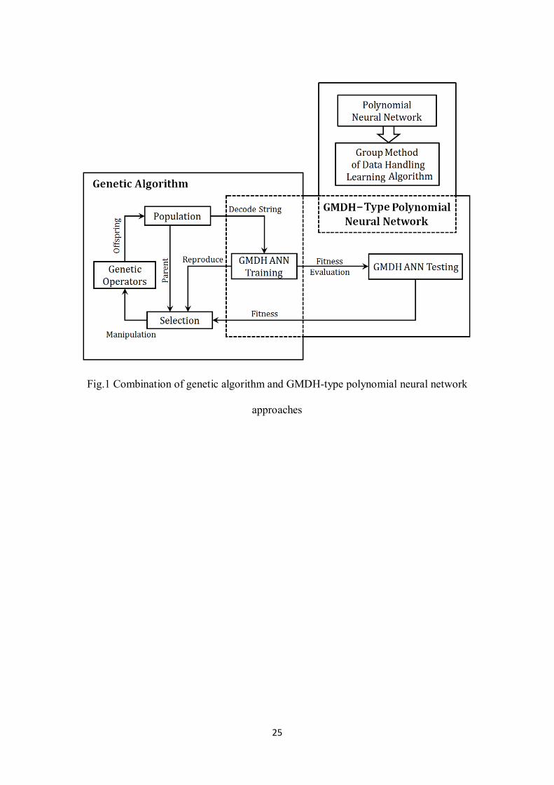
Genetic Optimisation of GMDH Polynomial Neural Networks

In this paper, a genetic algorithm is applied to determine the GMDH-type polynomial

neural network weights, hidden layers and bias coefficients for minimising the training

8

error and to find the optimal structure for a GMDH-type polynomial neural network.

The hidden layers and bias coefficients are different chromosomes that the genetic

algorithm tries to find. Fig. 1 shows the combination of the three different approaches

that were used to model thermal conductivity ratios in a hybrid system. By using a

group method of data handling learning algorithm to instruct the polynomial neural

network, the GMDH-type polynomial neural network which created the neural network

part was introduced. On the other hand, the genetic algorithm was used to find the

GMDH-type polynomial neural network hidden layers and bias coefficients. These three

different approaches built a genetic algorithm-GMDH-type polynomial neural network

hybrid system, which is called GA-PNN. The steps of this hybrid system approach are

described below:

Step 1: The number of chromosome strings was selected randomly and each of them

was divided into several sections. Each chromosome string was represented as a set of

the connection weights (hidden layer and bias coefficients) for the GMDH-type

polynomial neural network.

Step 2: For each string that was established with the training data, the fitness was

measured. A string’s probability of being selected for reproduction was proportional to

its fitness value.

Step 3: The crossover, mutation and mating operators create the offspring that constitute

the new generation. Decoding these new chromosomes, we gain a new set of weights

and then submit it to the network. If the training error meets the demand, then stop.

Step 4: In the last step, the chromosome string with the smallest error in the training

procedure was selected to provide the final network structure. After each run, a new set

of weights was obtained and replaced with the old set. Finally, one can get a best set of

9

weights (layer coefficients), and obtain a well-trained GMDH-type polynomial neural

network [19-20].

EFFECTIVE PARAMETERS

There are different effective parameters on nanofluids thermal conductivity reported in

literature, which can be used for modelling thermal conductivity ratios. Of these

parameters we chose three important ones for this study namely particle size, volume

concentration and temperature.

Effect of particle size

Chon et al. [21] measured the thermal conductivity of nanofluids containing three

different sizes of alumina nanoparticles with diameters of 11, 47 and 150 nm. Their

results showed that the thermal conductivity increased as particle size decreased. Li and

Peterson [22] observed up to 4% positive thermal conductivity enhancement for Al2O3-

water nanofluids containing 36 nm Al2O3 particles compared with nanofluids containing

47 nm Al2O3 particles at 2% volume concentration. Patel et al. [23] measured the

thermal conductivity of nanofluids containing different sizes of Al2O3, CuO, and Cu in

water, ethylene glycol and in transformer oil. They observed positive thermal

conductivity enhancements for Al2O3-water with smaller nanoparticles. For Al2O3-water

nanofluid at 2% volume concentration at 50 oC, the thermal conductivity enhancement

for the 11 nm sample (15.5%) was approximately double the enhancement for the 150

nm (7%) sample and about 1.5 times the enhancement for the 45 nm (10.5 %) sample.

10

Effect of volume concentration

Most of the nanofluids thermal conductivity data in the literature exhibited a linear

relationship with the particle volume concentration. However, some exceptions have

showed a non-linear relationship especially at low volume concentrations [24]. In these

studies, the slope of the thermal conductivity versus volume concentration can be

divided into two linear regimes. At low concentrations, the slope was greater than at

high concentrations. Most thermal conductivity data in the literature for Al2O3-water

nanofluids showed that with increasing nanoparticle volume concentration, the thermal

conductivity also increased [21-30], however, the intensity of the increase decreased for

the larger volume concentrations.

Effect of temperature

Das et al. [25] and Putra et al. [26] measured the thermal conductivity of nanofluids

containing Al2O3 at temperatures between 21 and 51ºC. They observed that the thermal

conductivity increased as the temperature increased. Over the limited temperature range

considered in their study, a gradual curve could appear linearly. Therefore, more

comprehensive data are required before concluding whether the thermal conductivity

exhibits a linear relationship with temperature. Chon et al. [21] reported thermal

conductivity measurements of water containing Al2O3 nanoparticles at temperatures

between 21 and 71ºC. They observed that the thermal conductivity increased as the

temperature increased. However, they also experienced that at 61 and 71ºC, the trend of

increasing thermal conductivity was not linear. Therefore, it can be concluded that the

temperature dependence of the thermal conductivity of nanofluids is dominant.

11

EXPERIMENTAL DATA USED FOR TRAINING AND TESTING PROCEDURE

Masuda et al. [2] were the first researchers who used nanoparticles for the enhancement

of heat transfer in a liquid. They used the transient hot wire technique to measure the

thermal conductivity ratios of Al2O3-water nanofluids. Their experiments included three

different temperatures, which were: 32, 47 and 67oC. Lee et al. [27] experimentally

investigated the thermal conductivity of Al2O3-water nanofluids prepared with 38.4 nm

average diameter of alumina nanoparticle at 21oC temperature for four different volume

concentrations (1, 2, 3 and 4%). Wang et al. [28] measured the effective thermal

conductivity of fluids and nanometer-size Al2O3 by using a steady-state parallel-plate

technique. They dispersed Al2O3 powder (γ phase) with an average diameter of 28 into

water with a vacuum pump fluid and measured the thermal conductivity ratio at 24oC in

three different volume concentrations. Das et al. [25] investigated the thermal

conductivity ratio of Al2O3-water nanofluids with a thermal oscillation method. They

studied the temperature effect of the thermal conductivity ratio of Al2O3 nanoparticles

with an average diameter of 38.4 nm. Their experiments consisted of seven different

temperatures (21, 26, 31, 36, 41, 46 and 51oC) for four nanoparticle volume

concentrations (1, 2, 3 and 4%). Putra et al. [26] reported some experimental data for

thermal conductivity ratio of Al2O3 (with an average diameter of 131.2 nm) in a water-

based nanofluid over a temperature range from 21 to 51oC at volume concentrations of 1

and 4%. Chon et al. [21] measured the thermal conductivity of Al2O3-water nanofluids

in 11, 47 and 150 nm nanoparticle sizes over a wide range of temperatures (from 21 to

71oC) at 1 and 4% volume concentrations. Li and Peterson [22, 29] published their

experimental investigation into the effect of variations in temperature and volume

concentration on steady-state effective thermal conductivity of Al2O3-water

12

suspensions. Al2O3 nanoparticles with 36 and 47 nm average diameters were blended

with water at 0.5, 2, 4, 6 and 10% volume concentrations and the resulting suspensions

were evaluated at temperatures ranging from 27.5 to 35.5oC. Kim et al. [30] measured

the thermal conductivity of alumina-water nanofluids by using the transient hot wire

method. They used alumina nanoparticles with an average diameter of 38 nm for their

work and reported the results for 0.3, 0.5, 0.8, 1.5, 2 and 3% of volume concentrations

at 25 oC. Timofeeva et al. [31] investigated Al2O3-water nanofluids thermal

conductivity for a series of nanofluids consisting of 11, 20 and 40 nm and volume

concentrations of 2.5, 5, 7.5 and 10% at 23oC. Zhang et al. [32] used a short hot wire

probe to measure the thermal conductivity ratio of Al2O3-water nanofluids for 10, 30

and 50oC. Ju et al. [33] reported their measurements for thermal conductivity of Al2O3-

water suspensions with nominal diameters of 20, 30 and 45 nm for volume

concentrations up to 10%. Murshed et al. [34] conducted an experimental investigation

into the effective thermal conductivity of Al2O3 nanoparticles with average diameters of

80 and 150 nm in a water-based suspension. In their work, the transient hot wire

technique was used to measure the thermal conductivity ratio of nanofluids at different

temperatures ranging from 21 to 60oC. Patel et al. [23] measured thermal conductivity

enhancement of Al2O3-water nanofluids in 11, 45 and 150 nm nanoparticle sizes for

four different temperatures (20, 30, 40 and 50 oC) at 0.5, 1, 2 and 3% volume

concentrations.

In this paper, all of the above experimental data were used to model the thermal

conductivity ratio (keff/kbf) of Al2O3-water nanofluids using the FCM-ANFIS and GA-

PNN approaches. Therefore, volume concentration ϕ, temperature T and nanoparticle

size PS were chosen as designing variables (input parameters) for the models.

13

RESULTS AND DISCUSSION

The performance of the FCM-ANFIS and the GA-PNN proposed models was tested

with the sum of the squares due to the error or summed squares of residuals (SSE) and

root mean square errors (RMSE). If Q1, Q2 , Q3 , …, Qn are n observed values, P1, P2 ,

P3 , …, Pn are n predicted values, then SSE and RMSE values are as follows:

= ( − )(6)

=1

. ( − )

(7)

A total of 125 input output experimental data points obtained from literature were used

for three effective input parameters (volume concentration ϕ, temperature T and

nanoparticle size PS). These data were divided into two subsets as 80% for training and

20% for testing purposes. The characterisation of the FCM-ANFIS model is shown in

Table 1. The structure of the GA-PNN model is shown in Fig. 2 corresponding to the

genome representation of 2312332311231322 for thermal conductivity ratio (keff/kbf) in

which 1, 2 and 3 stand for volume concentration ϕ (%), temperature T (oC) and

nanoparticle size PS (nm), respectively. The corresponding polynomial representation

of models for keff/kbf is shown in the appendix.

Two statistical criteria which were mentioned before, were used to determine how well

the FCM-ANFIS and GA-PNN models could predict the thermal conductivity ratio

keff/kbf of Al2O3-water nanofluids corresponding to various values of inlet variables.

Figures 3-7 show plots comparing the experimental data, FCM-ANFIS and GA-PNN

models. These diagrams demonstrate that the predicted values are close to the

14

experimental data, as many of the modelled data points fall very close to the

experimental value.

Fig. 3 shows the experimental results of Lee et al. [27] compared with the FCM-ANFIS

and the GA-PNN models for a particle size of 38.4 nm, temperature of 21oC at four

different volume concentrations. The GA-PNN model is in very good agreement with

the experimental data (SSE =1.527 × 10 and RMSE = 0.002). Therefore, the GA-

PNN model is well matched with the experimental data. The FCM-ANFIS (SSE

=2.237 × 10 and RMSE = 0.0011) model is not as good as the GA-PNN model.

Although the FCM-ANFIS model is not well matched with the experimental data, the

maximum relative error is less than 2.5%.

Fig. 4 shows the experimental results of Putra et al. [26] compared with the FCM-

ANFIS and the GA-PNN models for a particle size of 131.2 nm, volume concentration

of 1% and seven different temperatures. The GA-PNN model is in good agreement with

the experimental data (SSE =1.887 × 10 and RMSE = 0.0061), the difference

between the model outputs and experimental results is less than 4%. The FCM-ANFIS

model is in very good agreement with experimental results at higher temperatures from

36-51oC (SSE =2.006 × 10 and RMSE =0.002) but for temperatures between 21-

36oC the FCM-ANFIS model is not as good as the higher temperatures. However, the

maximum difference between the experimental data and the FCM-ANFIS model at the

lowest temperature of 21oC is about 3%.

In Fig. 5, the experimental results of Li and Peterson [22] compared with the FCM-

ANFIS and the GA-PNN models are presented for a particle size of 36 nm, temperature

of 30.5oC at four different volume concentrations. The FCM-ANFIS model (SSE

15

=3.582 × 10 and RMSE =0.0004) is well matched and the GA-PNN model (SSE

=6.132 × 10 and RMSE =0.0018) is also in good agreement with the experimental

data. For the FCM-ANFIS model at ϕ= 2% and ϕ=6%, the model is approximately the

same as the experimental data.

Fig. 6 shows the experimental results of Kim et al. [30] compared with the FCM-

ANFIS and the GA-PNN models for a particle size of 38 nm, temperature of 25 oC at

five different volume concentrations. The FCM-ANFIS model (SSE =8.39 × 10 and

RMSE =0.0046) and the GA-PNN model (SSE =3.576 × 10 and RMSE =0.0029) are

in good agreement with the experimental data. However, as the volume concentration

increases, the accuracy of the FCM-ANFIS is better than that of the GA-PNN model.

In Fig. 7, the experimental results of Patal et al. [23] is compared with those of the

FCM-ANFIS and the GA-PNN models for a particle size of 150 nm, volume

concentration of 2% at four different temperatures. The FCM-ANFIS model matches

the data very well (SSE =3.179 × 10 and RMSE = 0.0126). However, the GA-PNN

model (SSE = 0.0026 and RMSE = 0.0361) is not in such a good agreement with the

experimental data and the difference between this model and GA-PNN output for

T=50oC is about 6%.

16

CONCLUSIONS

This study showed the high capability of artificial intelligent methods for modelling

engineering problems containing nanofluids based on input output experimental data,

which were published in literature, for this purpose, the FCM-ANFIS and the GA-PNN

approaches were developed for modelling the thermal conductivity ratio of Al2O3-water

nanofluids as function of particle size, temperature and volume concentration.

In the FCM-ANFIS method, which consists of a neural network combined with a fuzzy

logic approach, the fuzzy C-means clustering is used as an identification method. The

Adaptive Neuro-Fuzzy Inference System (ANFIS) uses neural network and fuzzy logic

approaches at the same time to combine the advantages of each method to achieve a

better performance. In the GA-PNN hybrid system, which consists of neural network

and genetic algorithm parts, the genetic algorithm is used to find the best network

weights for minimising the training error and finding the optimal structure for a

GMDH-type polynomial neural network. In the neural network part of this hybrid

system the Group Method of Data Handling (GMDH) learning approach is used to learn

a second rate polynomial neural network.

After a literature review of experimental works on Al2O3-water nanofluids thermal

conductivity, we chose particle size, temperature and volume concentration as most

effective parameters of thermal conductivity ratio. After choosing these effective (input)

parameters, we used 125 input output experimental data points obtained from literature

to model the thermal conductivity ratio by using the FCM-ANFIS and GA-PNN

approaches. The characterisation of the FCM-ANFIS model with detailed information is

mentioned in a table. The structure of the GA-PNN model based on the genome

17

representation for thermal conductivity ratio with respect to effective (input) parameters

is shown in a figure.

The result statistical error analyses review shows that our proposed models are in good

agreement compared with experimental data. Although the FCM-ANFIS approach

shows better agreement with experimental data in comparison with the GA-PNN

method, the differences between the GA-PNN model outputs and experimental results

in the worst-case scenario are about 6%.

REFERENCES

[1] R. Saidur, K.Y. Leong, H.A. Mohammad, A review on applications and challenges

of nanofluids, Renewable and Sustainable Energy Reviews 15 (2011) 1646–1668.

[2] H. Masuda, A. Ebata, K. Teramae, N. Hishinuma, Alteration of thermal conductivity

and viscosity of liquid by dispersing ultra-fine particles (dispersion of c-Al2O3, SiO2 and

TiO2 ultra-fine particles), Netsu Bussei 4 (1993) 227–233.

[3] S.U.S. Choi, Enhancing thermal conductivity of fluids with nanoparticles. ASME

FED 231 (1995) 99–103.

[4] C. Kleinstreuer, Y. Feng, Experimental and theoretical studies of nanofluid thermal

conductivity enhancement: a review, Nanoscale Research Letters 6 (2011) 229.

[5] A. Kargar, B. Ghasemi, S.M. Aminossadati, An artificial neural network approach to

cooling analysis of electronic components in enclosures filled with nanofluids, Journal

of Electronic Packaging, 131(2011) 011010-1.

18

[6] M. Hojjat, S.Gh. Etemad, R. Bagheri, J. Thibault, Thermal conductivity of non-

Newtonian nanofluids: Experimental data and modeling using neural network,

International Journal of Heat and Mass Transfer 54 (2011) 1017–1023.

[7] M.M. Papari, F.Yousefi, J. Moghadasi, H. Karimi, A. Campo, Modeling thermal

conductivity augmentation of nanofluids using diffusion neural networks, International

Journal of Thermal Sciences 50 (2011) 44-52.

[8] M. Mehrabi, S.M. Pesteei, T. Pashaee G., Modeling of heat transfer and fluid flow

characteristics of helicoidal double-pipe heat exchangers using Adaptive Neuro-Fuzzy

Inference System (ANFIS), International Communications in Heat and Mass Transfer

38 (4) (2011) 525-532.

[9] H. Jalalifar, S. Mojedifar, A.A. Sahebi, H. Nezamabadi-pour, Application of the

adaptive neuro-fuzzy inference system for prediction of a rock engineering

classification system, Computers and Geotechnics 38 (2011) 783–790.

[10] J.C. Bezdek, Fuzzy Mathematics in Pattern Classification. PhD dissertation,

Cornell University, Ithaca, NY, 1973.

[11] S.S. Kim, D.J. Lee, K.C. Kwak, J.H. Park, J.W. Ryu, Speech recognition using

integra-normalizer and neuro-fuzzy method, Conference Record of the Asilomar

Conference on Signals, Systems and Computers 2 (2000) 1498-1501.

[12] M.F. Othman, T. Moh, Neuro Fuzzy Classification and Detection Technique for

Bioinformatics Problems, Proceedings of the First Asia International Conference on

Modelling & Simulation (AMS'07) 0-7695-2845-7/07 375-380.

19

[13] S. Ibrahim, N.E.A. Khalid, M. Manaf, Seed-Based Region Growing (SBRG) vs

Adaptive Network-Based Inference System (ANFIS) vs Fuzzy c-Means (FCM): Brain

Abnormalities Segmentation, Proceedings of World Academy of Science, Engineering

and Technology 68 (2010) 425-435.

[14] A.G. Ivakhnenko, Polynomial Theory of Complex Systems, IEEE Transaction on

Systems, Man and Cybernetics SMC-1 (4) (1971) 364-378.

[15] A.G. Ivakhenko, G.A. Ivakhenko, the Review of Problems Solvable by Algorithms

of Group Method of Data Handling, Pattern Recognition and Image Analysis 5(4)

(1995) 527-535.

[16] A.G. Ivakhnenko, the Group Method of Data Handling - A Rival of the Method of

Stochastic Approximation, Soviet Automatic Control 13 (3) (1966) 43-55.

[17] K. Fujimoto, S. Nakabayashi, Applying GMDH algorithm to extract rules from

examples, Systems Analysis Modelling Simulation 43 (10) (2003) 1311-1319.

[18] F. Lemke, J.A. Müller, Self-organizing data mining, Systems analysis modelling

simulation 43(2) (2003) 231–240.

[19] M. Saemi, M. Ahmadi, A. Yazdian Varjani, Design of neural networks using

genetic algorithm for the permeability estimation of the reservoir, Journal of Petroleum

Science and Engineering 59 (2007) 97–105.

[20] N.Y. Nikolaev, H. Iba, Learning polynomial feedforward neural networks by

genetic programming and backpropagation, IEEE Transactions on Neural Networks,

14(2) (2003) 337-350.

20

[21] C.H. Chon, K.D. Kihm, S.P. Lee, S.U.S. Choi, Empirical correlation finding the

role of temperature and particle size for nanofluid (Al2O3) thermal conductivity

enhancement, Applied Physics Letters 87 (2005) 153107.

[22] C.H. Li, G.P. Peterson, The effect of particle size on the effective thermal

conductivity of Al2O3-water nanofluids, Journal of Applied Physics 101 (2007) 044312.

[23] H.E. Patel, T. Sundararajan, S.K. Das, An experimental investigation into the

thermal conductivity enhancement in oxide and metallic nanofluids, Journal of

Nanoparticle Research 12 (2010) 1015–1031.

[24] S.M.S. Murshed, K.C. Leong, C. Yang, Enhanced thermal conductivity of TiO2 -

water based nanofluids. International Journal of Thermal Sciences 44(4) (2005) 367-

373.

[25] S.K. Das, N. Putra, P. Thiesen, W. Roetzel, Temperature dependence of thermal

conductivity enhancement for nanofluids, Journal of Heat Transfer 125 (2003) 567–

574.

[26] N. Putra, W. Roetzel, S.K. Das, Natural convection of nano-fluids, Heat and Mass

Transfer 39 (2003) 775–784.

[27] S. Lee, S.U.S. Choi, S. Li, J.A. Eastman, Measuring thermal conductivity of fluids

containing oxide nanoparticles, Journal of Heat Transfer 121(2) (1999) 280-289.

[28] X. Wang, X. Xu, S.U.S. Choi, Thermal conductivity of nanoparticle–fluid mixture,

Journal of Thermophysics and Heat Transfer 13(4) (1999) 474–480.

21

[29] C.H. Li, G.P. Peterson, Experimental investigation of temperature and volume

fraction variations on the effective thermal conductivity of nanoparticle suspensions

(nanofluids), Journal of Applied Physics 99 (2006) 084314.

[30] S.H. Kim, S.R. Choi, D. Kim, Thermal conductivity of metal-oxide nanofluids:

particle size dependence and effect of laser irradiation, Journal of Heat Transfer 129

(2007) 298-307.

[31] E.V. Timofeeva, A.N. Gavrilov, J.M. McCloskey, Y.V. Tolmachev, Thermal

conductivity and particle agglomeration in alumina nanofluids: experiment and theory,

Physical Review E 76 (2007) 061203.

[32] X. Zhang, H. Gu, M. Fujii, Effective thermal conductivity and thermal diffusivity

of nanofluids containing spherical and cylindrical nanoparticles, Experimental Thermal

and Fluid Science 31 (2007) 593–599.

[33] Y.S. Ju, J. Kim, M.T Hung, Experimental Study of Heat Conduction in Aqueous

Suspensions of Aluminium Oxide Nanoparticles, Journal of Heat Transfer 130 (2008)

092403-1.

[34] S.M.S. Murshed, K.C. Leong, C. Yang, Investigations of thermal conductivity and

viscosity of nanofluids, International Journal of Thermal Sciences 47 (2008) 560–568.

22

NOMENCLATURE

kPPSQTvmcUuijJZMxaiLij

Thermal conductivity (W/mK)Predicted valueNanoparticle size (nm)Observed valueTemperature (oC)Number of clustersWeighting exponent (fuzziness index)Cluster centresMembership matrixMembership functionObjective functionGMDH processor unit outputNumber of input variable to each GMDH processor unitData pointPolynomial coefficient (weight)i-th output in j-th layer for GA-PNN model

Greek lettersϕ Volume concentration (%)

Subscriptseffbf

EffectiveBase fluid

Abbreviation

FCM-ANFISGA-PNNGMDHSSERMSE

FCM-based Neuro-Fuzzy Inference SystemGenetic Algorithm-GMDH Polynomial Neural NetworkGroup Method of Data HandlingSum of squares due to error or summed square of residualsRoot mean square error

23

Appendix:

= , + , . + , . + , . . + , . + , .

= , + , . + , . + , . . + , . + , .

= , + , . + , . + , . . + , . + , .

= , + , . + , . + , . . + , . + , .

= , + , . + , . + , . . + , . + , .

= , + , . + , . + , . . + , . + , .

= , + , . + , . + , . . + , . + , .

= , + , . + , . + , . . + , . + , .

= , + , . + , . + , . . + , . + , .

= , + , . + , . + , . . + , . + , .

, =

⎣⎢⎢⎢⎢⎢⎢⎢⎢⎡

1.0735962 −0.0020244 0.0605055 8.35 × 100.8718401 0.0098069 0.0011233 −7.83 × 100.8733007 0.0069859 0.0177932 −7.08 × 1010.668079 −15.644669 −3.3349184 3.9400101−2.6847113 −0.3084822 6.3004023 −1.26 × 103.4734893 −0.0050944 −5.2272048 −9.32 × 10

0.4093305 0.4501285 −0.0042521 0.19896110.9721418 −2.0553909 1.2665332 −2.3233686

−0.0064905−7.14 × 10−2.67 × 10−1.6277918−2.59001012.5841052

6.83 × 10−4.1070767

0.0001505−7.75 × 107.96 × 107.00654010.27600020.01405290.00251857.2531441

0.2394494 2.1513521 −1.5733885 13.480884 15.199995 −28.498592−0.0477731 1.0660376 −0.0012041 0.0495427 0.7246142 −0.7942074 ⎦

⎥⎥⎥⎥⎥⎥⎥⎥⎤

24

Table 1Different parameter types and their values used for training FCM-ANFIS

Parameters FCM-ANFIS

Membership functions type

Number of membership functions

Output membership functions

Number of nodes

Number of linear parameters

Number of non-linear parameters

Number of training data pairs

Number of fuzzy rules

Gaussian

6

Linear

54

24

36

125

6

25

Fig.1 Combination of genetic algorithm and GMDH-type polynomial neural network

approaches

26

Fig.2 Structure of GA-PNN-type neural network for thermal conductivity ratio (keff/kbf)

modelling

Fig.3 Comparison between the experimental data of Lee et al. [27] and the proposed

models for PS= 38.4 nm and T= 21oC

0.96

1

1.04

1.08

1.12

1 2 3 4

Ther

mal

cond

uctiv

ity ra

tio

Volume concentration (%)

FCM-ANFISGA-PNNExperimental Data

27

Fig.4 Comparison between the experimental data of Putra et al. [26] and the proposed

models for PS= 131.2 nm and ϕ= 1%

Fig.5 Comparison between the experimental data of Li and Peterson [22] and the

proposed models for PS= 36 nm and T= 30.5oC

0.92

0.96

1

1.04

1.08

1.12

21 26 31 36 41 46 51

Ther

mal

cond

uctiv

ity ra

tio

Temperature (C)

FCM-ANFISGA-PNNExperimental Data

0.95

1

1.05

1.1

1.15

1.2

0 2 4 6

Ther

mal

cond

uctiv

ity ra

tio

Volume concentration (%)

FCM-ANFISGA-PNNExperimental Data

28

Fig.6 Comparison between the experimental data of Kim et al. [30] and the proposed

models for PS= 38 nm and T= 25oC

Fig.7 Comparison between the experimental data of Patal et al. [23] and the proposed

models for PS= 150 nm and ϕ= 2%

0.96

0.98

1

1.02

1.04

1.06

1.08

1.1

0.5 1 1.5 2 2.5 3

Ther

mal

cond

uctiv

ity ra

tio

Volume concentration (%)

FCM-ANFISGA-PNNExperimental Data

0.92

0.96

1

1.04

1.08

1.12

1.16

20 30 40 50

Ther

mal

cond

uctiv

ity ra

tio

Temperature (C)

FCM-ANFISGA-PNNExperimental Data