SLAC - PUB - 4669 July 1988 (T/E)

APPLICATION OF THE BOOTSTRAP STATISTICAL METHOD TO THE TAU DECAY MODE PROBLEM*

KENNETH G. HAYES AND MARTIN L. PERL

Stanford Linear Accelerator Center Stanford University, Stanford, California 94309

BRADLEY EFRON *

Department of Statistics P Stanford University, Stanford, California 94309

ABSTRACT

The bootstrap statistical method is applied to the discrepancy in the

l-charged particle decay modes of the tau lepton. This eliminates questions about

the correctness of the errors ascribed to the branching fraction measurements and

the use of gaussian error distributions for systematic errors. The discrepancy is

still seen when the results of the bootstrap analysis are combined with other

measurements and with deductions from theory. But the bootstrap method as-

signs less statistical significance to the discrepancy compared to a method using

gaussian error distributions.

Submitted to Physical Review D

* This work was supported by the Department of Energy, contract DE-AC03-76SF00515, and the National Science Foundation, grant DMS 86-00235.

I. INTRODUCTION

At present there is a problem1*2] in fully understanding the decay modes of

the tau lepton to l-charged particle. The average directly measured value11 of the

inclusive, l-charged particle, branching fraction, Br, is (86.6 f 0.3)%. The same

number should be obtained by adding up the branching fractions of the individual

l-charged particle modes. Examples of these individual branching fractions are:

B,: r- + u, + e- + De

B cc: r- --+ lJr + p- + $

B,: r--+vz+~-

P B PZ r- --+ur+p- +u,+7r-+7r”

B r2ro : r- + UT + ?r- + 27r”

B r3ro : r- + u, + 7r- + 37r”

As shown in Table 1 from Ref. 2, this sum is less than (80.6 f 1.5)%, 6% less

than the directly measured value of B1. This is the r decay mode problem.

Attempts to resolve the problem include: questioning’] the errors ascribed

by the experimenters to Bl, B, B,, B, and BP; searching for bias in the

measurementsl]; questioning the theory used to derive upper limits; and searching

for unconventional explanations.2] The error and bias studies in Ref. 1 assumed

the errors are gaussian distributed, an assumption which cannot be justified for

systematic errors. In this paper we apply the bootstrap3*4] method of statistical

analysis which does not use the ascribed errors.

The bootstrap method, Sec. II, requires multiple measurements of a quantity.

We can apply it to B1 , Be, B,, B,, and BP which have been repeatedly measured,

2

Tables 2-6 and Sec. III. But we cannot apply it to the smaller branching fractions

such as Brzro and Brzro, which have few or no measurements. The branching

fraction for the l-charged particle decay modes containing K mesons is based

on a few connected measurements, and is again not suitable for the bootstrap

method. Fortunately this branching fraction is small.

In Sec. IV we apply the bootstrap method to the quantity

AB = Bl - (BP + B, + B, + B,) ,

obtaining means and confidence levels for AB. We compare these findings with

the upper limit on AB given by the sums of the branching fractions in rows . 3 and 4 of Table 1. This comparison is done in Sec. V. We find that there is

still a discrepancy in understanding the l-charged particle decay modes, but the

discrepancy is less striking than when studied using normal error analysis.ll

II. THE BOOTSTRAP STATISTICAL METHOD

Consider a set of N measurements yr, y2 . . . ye of a quantity y. Randomly

select one of the set, note it, and replace it in the set. Carry out N such random

selections with replacement forming a bootstrap replication set, r(l), with N

members: y[, yl . . . y;. Some of the yn will appear as several yi’s, some yn

will not appear at all in r(1). Let g*(l) be the mean value of the y;‘s in r(1)

calculated by giving each yi the weight l/N.

In the simplest form of the bootstrap method this replication is carried out

R times, constructing sets r(l), r(2) . ..r(R) with means g*(l), g*(2) . ..fj*(R).

From these sets one directly calculates various properties of the distribution of

3

the R means, properties such as the standard deviation of the mean and various

confidence intervals for the mean. Thus the errors assigned by the experimenters

to their measurements are not used in this analysis. References 3 and 4 give a

general description and a technical description of the bootstrap method.

In this paper we use the trimmed mean concept. Consider a bootstrap repli-

cation set, r(i), with N members y;, y$ . . . y& now ordered in size from smallest

to largest. Select a fraction f with 0 5 f 5 0.5, and remove the jN smallest val-

ues of y,*l and the jN largest values of yi. The mean of the (1 - 2f)N remaining

values of yk is the f trimmed mean. The case f = l/2 gives%the median. This

procedure reduces the sensitivity of the mean to outlying values of yl.

Our analyses are based on f = 0.25, a 25% trimmed mean. The selection of

f = 0.25 comes from a study of the effect of various f values on the analyses.

III. BRANCHING FRACTION MEASUREMENTS

The branching fraction measurements are given in Tables 2-5 taken from

Ref. 1. In Ref. 1 all published measurements of B1 , BP, B,, B,, and B, are

listed, including several published measurements partially based on the same

data. Here we use the most complete measurement of such a set.

Table 2 gives 11 measurements of Bl. Measurements published before 1982

are not used for reasons given in Ref. 1. Tables 3 and 4 give 6 measurements of

BP and 7 measurements of B,.

Some of the leptonic branching fraction measurements, B, and B,, are com-

plicated by the conventionally accepted existence of the universality relation

B, = 0.973 B, , (1)

4

or by strongly correlated errors in the two measurements. Therefore the mea-

surements are divided into two groups. Table 5a lists 14 measurements with

independent values of B, and B,. Table 5b lists 7 measurements constrained by

Eq. 1 or highly correlated.

IV. ANALYSES

We have conducted two conventional bootstrap analyses of the measurements,

the two differing in how B, and B, are treated. We have also conducted one

unconventional bootstrap analysis using weighted mneasurements.

A. Analysis Ignoring Correlations Between B, and B, _

In this analysis we ignored the correlations between the Be and B, measure-

ments in Table 5b, treating those measurements the same as the independent

measurements in Table 5a. This gave 14 values of Be and 20 values of BP. Our

first step was to produce 500 bootstrap replications of the five branching fractions

Bl, BP, B, B,, and B,. The means and standard deviations of the bootstrap

25% trimmed means are in Table 6.

The second step in the analysis was to produce 2000 bootstrap replications

of AB obtained by sampling 2000 times from the 500 bootstrap means of Be,

the 500 bootstrap means of BP, and so forth. This gave the 25% trimmed mean

and the bootstrap confidence levels of AB in Table 7. (The bootstrap confidence

level is a bias corrected percentile confidence leve13141.)

B. Analysis Using Correlations Between B, and B,

Next we took account of the correlations between the 7 (B,, B,) measure-

ments in Table 5b. The bootstrap replication sets for B, and B, were constructed

5

by first drawing with replacement 7 (B,, B,) pairs from Table 5b. Then 7 B,

samples were drawn with replacement from Table 5a. Similarly 13 BP samples

were drawn from Table 5a. Thus a B, replication set with 14 values was formed

and a B, set with 20 values was formed. As before we produced 500 bootstrap

replication sets of B, and B,.

These 500 new sets of B, and B, were combined with the previous 500 sets

of B1, BP, and B, to make 2000 bootstrap replications of AB. The properties

of this sample of 2000 values of AB are given in Table 7. Taking account of the

(Be, B,) correlations in Table 5b has a negligible effect on the confidence level

intervals.

C. Analyses Using Weighted Measurements

Although one strength of the bootstrap method is its independence from error

estimation for individual measurements, it is interesting to investigate the effect

of using the individual errors to weight the measurements. Tables 2-5 give the

statistical, systematic, and combined errors quoted by experimenters for their

own measurement. Calling ai the combined error for measurement i, the relative

weight is l/o:. We used these weights in the bootstrap analysis by finding a

constant C such that an interger

ni - C/of (2)

is associated with measurement i. We then formed a larger measurement set

with measurement i repeated ni times.

Using the enlarged measurement sets, 200 bootstrap replication sets were

produced for Bl, BP, &, Be, and BP. (The correlations in Table 5b were

6

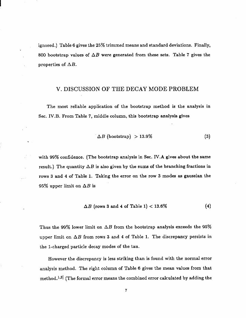
ignored.) Table 6 gives the 25% trimmed means and standard deviations. Finally,

800 bootstrap values of AB were generated from these sets. Table 7 gives the

properties of AB.

V. DISCUSSION OF THE DECAY MODE PROBLEM

The most reliable application of the bootstrap method is the analysis in

Sec. 1V.B. From Table 7, middle column, this bootstrap analysis gives

-AB (bootstrap) > 13.9% (3)

with 99% confidence. (The bootstrap analysis in Sec. IV.A gives about the same

result.) The quantity AB is also given by the sums of the branching fractions in

rows 3 and 4 of Table 1. Taking the error on the row 3 modes as gaussian the

95% upper limit on AS is

AB (rows 3 and 4 of Table 1) < 13.6% (4

Thus the 99% lower limit on AB from the bootstrap analysis exceeds the 95%

upper limit on AB from rows 3 and 4 of Table 1. The discrepancy persists in

the l-charged particle decay modes of the tau.

However the discrepancy is less striking than is found with the normal error

analysis method. The right column of Table 6 gives the mean values from that

method.lp21 (The formal error means the combined error calculated by adding the

7

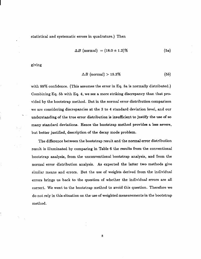
statistical and systematic errors in quadrature.) Then

AB (normal) = (18.0 f 1.2)% (54

giving

AB (normal) > 15.3% (54

with 99% confidence. (This assumes the error in Eq. 5a is normally distributed.)

Combining Eq. 5b with Eq. 4, we see a more striking discrepancy than that pro-

vided by the bootstrap method. But in the normal error distribution comparison

we are considering discrepancies at the 3 to 4 standard deviation level, and our P

understanding of the true error distribution is insufficient to justify the use of so

many standard deviations. Hence the bootstrap method provides a less severe,

but better justified, description of the decay mode problem.

The difference between the bootstrap result and the normal error distribution

result is illuminated by comparing in Table 6 the results from the conventional

bootstrap analysis, from the unconventional bootstrap analysis, and from the

normal error distribution analysis. As expected the latter two methods give

similar means and errors. But the use of weights derived from the individual

errors brings us back to the question of whether the individual errors are all

correct. We went to the bootstrap method to avoid this question. Therefore we

do not rely in this situation on the use of weighted measurements in the bootstrap

method.

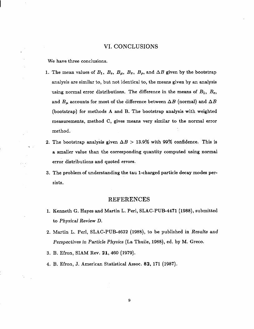
VI. CONCLUSIONS

We have three conclusions.

1. The mean values of Bl, B,, B,, B,, BP, and AB given by the bootstrap

analysis are similar to, but not identical to, the means given by an analysis

using normal error distributions. The difference in the means of Bl, B,,

and B, accounts for most of the difference between AB (normal) and AB

(bootstrap) for methods A and B. The bootstrap analysis with weighted

measurements, method C, gives means very similar to the normal error

method.

2. The bootstrap analysis given AB > 13.9% with 99% confidence. This is

a smaller value than the corresponding quantity computed using normal

error distributions and quoted errors.

3. The problem of understanding the tau l-charged particle decay modes per-

sists.

REFERENCES

1. Kenneth G. Hayes and Martin L. Perl, SLAC-PUB-4471 (1988), submitted

to Physical Review D.

2. Martin L. Perl, SLAC-PUB-4632 (1988), to be published in Results and

Perspectives in Particle Physics (La Thuile, 1988), ed. by M. Greco.

3. B. Efron, SIAM Rev. 21,460 (1979).

4. B. Efron, J. American Statistical Assoc. 82, 171 (1987).

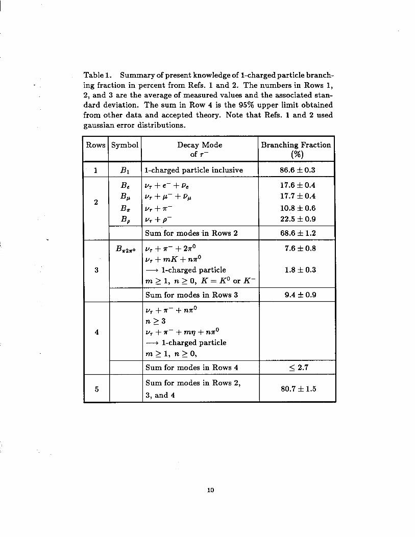
Table 1. Summary of present knowledge of l-charged particle branch- ing fraction in percent from Refs. 1 and 2. The numbers in Rows 1, 2, and 3 are the average of measured values and the associated stan- dard deviation. The sum in Row 4 is the 95% upper limit obtained from other data and accepted theory. Note that Refs. 1 and 2 used gaussian error distributions.

.

Decay Mode Branching Fraction of r- m

1 I Bl I l-charged particle inclusive I 86.6 f 0.3

B, ur + e- + De 17.6 f 0.4

2 BP UT -I- p- -I- pi,4 17.7 f 0.4 BU u,+?r- 10.8 f 0.6 B, b+P- 22.5 f 0.9

I I Sum-for modes in Rows 2 1 68.6 f 1.2

B s2ro u, + 7r- + 27ro 7.6 f 0.8 u,+mK+n~”

3 _+ l-charged particle 1.8 f 0.3 m>l, n>O, K=KOorK-

I I Sum for modes in Rows 3 I 9.4 f 0.9

4 4

u,+7r-+n7r” u,+7r-+n7r” n>3 n>3 uT+7r-+mq+n7ro uT+7r-+mq+n7ro + l-charged particle + l-charged particle m 2 1, n 2 0, m 2 1, n 2 0,

I Sum for modes in Rows 4 I 5 2.7

5 I I Sum for modes in Rows 2, 80.7 f 1.5

3, and 4

10

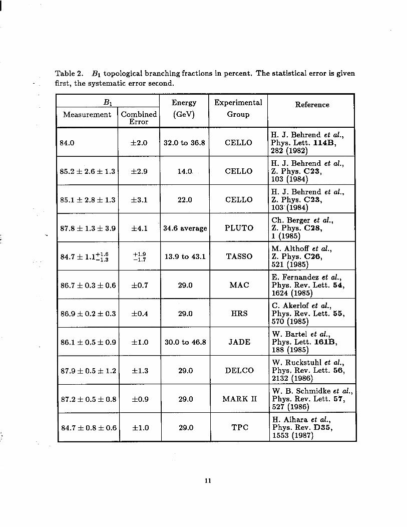
Table 2. B1 topological branching fractions in percent. The statistical error is given first, the systematic error second.

P

Bl Measurement Combined

Error

Energy Experimental

(GW Group Reference

H. J. Behrend et al., 84.0 f2.0 32.0 to 36.8 CELLO Phys. Lett. 114B,

282 (1982) H. J. Behrend et al.,

85.2 f 2.6f 1.3 f2.9 14.0 CELLO 2. Phys. C23, 103 (1984) H. J. Behrend et al.,

85.lf 2.8 f 1.3 f3.1 22.0 CELLO Z. Phys. C23, 103’( 1984) Ch. Berger et al.,

87.8 f 1.3 f 3.9 f4.1 34.6 average PLUTO Z. Phys. C28, 1 (1985)

84.7 f 1.12;:; +1.9 M. Althoff et al.,

-1.7 13.9 to 43.1 TASS0 Z. Phys. C26, 521 (1985)

E. Fernandez et al., 86.7 f 0.3 f 0.6 f0.7 29.0 MAC Phys. Rev. Lett. 54,

1624 (1985) C. Akerlof et cd.,

86.9 f 0.2 f 0.3 f0.4 29.0 HRS Phys. Rev. Lett. 55, 570 (1985) W. Bartel et al.,

86.1 f 0.5 f 0.9 fl.O 30.0 to 46.8 JADE Phys. Lett. 161B, 188 (1985) W. Ruckstuhl et al.,

87.9 f 0.5 f 1.2 f1.3 29.0 DELCO Phys. Rev. Lett. 56, 2132 (1986) W. B. Schmidke et al.,

87.2 f 0.5 f 0.8 f0.9 29.0 MARK II Phys. Rev. Lett. 57, 527 (1986) H. Aihara et al.,

84.7 f 0.8 f 0.6 fl.O 29.0 TPC Phys. Rev. D35, 1553 (1987)

11

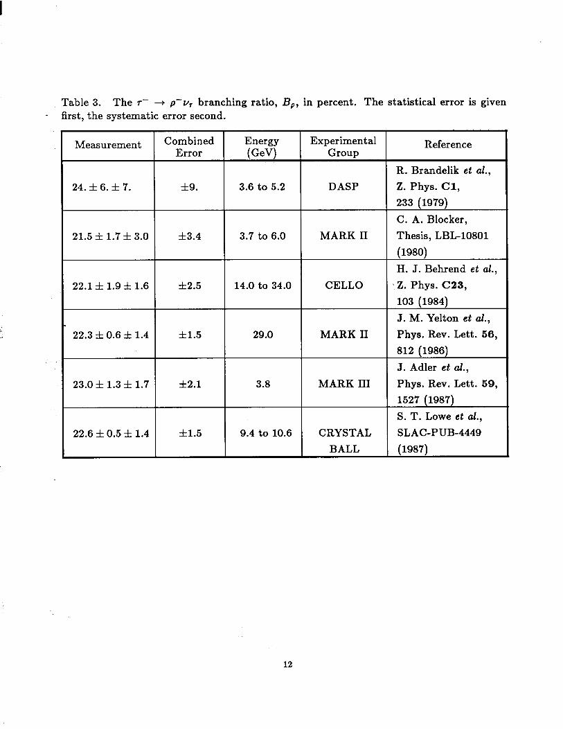
Table 3. The r- + p-u, branching ratio, BP, in percent. The statistical error is given - first, the systematic error second.

Measurement Combined Energy Error PV)

Experimental Group

Reference

R. Brandelik et al., 24. f 6. f 7. f9. 3.6 to 5.2 DASP Z. Phys. Cl,

233 (1979) C. A. Blocker,

21.5 f 1.7 f 3.0 f3.4 3.7 to 6.0 MARK II Thesis, LBL-10801 (1980) H. J. Behrend et al.,

22.1 f 1.9 f 1.6 f2.5 14.0 to 34.0 CELLO * Z. Phys. C23, 103 (1984) J. M. Yelton et al.,

22.3 f 0.6 f 1.4 f1.5 29.0 MARK II Phys. Rev. Lett. 56, 812 (1986) J. Adler et al.,

23.0 f 1.3 f 1.7 f2.1 3.8 MARK III Phys. Rev. Lett. 59, 1527 (1987) S. T. Lowe et al.,

22.6 f 0.5 f 1.4 f1.5 9.4 to 10.6 CRYSTAL SLAC-PUB-4449 BALL (1987)

12

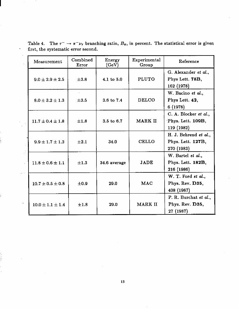
Table 4. The r- --) ?r-ur branching ratio, B,, in percent. The statistical error is given first, the systematic error second.

Measurement

9.0 f 2.9 f 2.5

8.0 f 3.2 f 1.3

11.7 f 0.4 f 1.8

9.9 f 1.7 f 1.3

11.8 f 0.6 f 1.1

10.7f0.5 f 0.8

10.0 f 1.1 f 1.4

Combined Error

f3.8

Energy PV)

4.1 to 5.0

f3.5 3.6 to 7.4

f1.8 3.5 to 6.7

f2.1 34.0

f1.3 34.6 average

f0.9 29.0

f1.8 29.0

Experimental Reference Group

G. Alexander et al., PLUTO Phys Lett. 78B,

162 (1978) W. Bacino et al.,

DELCO Phys Lett. 42, 6 (1978) C. A. Blocker et al.,

MARK II *Phys. Lett. 109B, 119 (1982) H. J. Behrend et al.,

CELLO Phys. Lett. 127B, 270 (1983) W. Bartel et al.,

JADE Phys. Lett. 182B, 216 (1986) W. T. Ford et al.,

MAC Phys. Rev. D35, 408 (1987) P. R. Burchat et al.,

MARK II Phys. Rev. D35, 27 (1987)

13

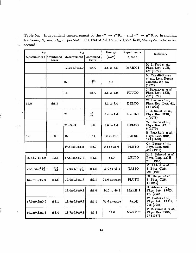
Table 5a. Independent measurement of the F ---) e-Deu7 and T- + ~-D,,u, branching fractions, B, and B,, in percent. The statistical error is given first, the systematic error second.

Be BP Energy Experimental Reference vleasurement Combined Measurement Combined (GeV) Group

Error Error M. L. Per1 et al.,

17.5f2.7f3.0 f4.0 3.8 to 7.8 MARK I Phys. Lett. 70B, 487 (1977) M. Cavalli-Storza et al.,, Lett. Nuovo

22. +10. -7. 4.8 Cimento 20, 337

(1977) J. Burmester et al.,

15. f3.0 3.6 to 5.0 PLUTO Phys. Lett. 68B, 297 (1977) W. Bacino et al.,

.6.0 *1.3 3.1 to 7.4 DELCO Phys. Rev. Lett. 41, 13 (1978) J. G. Smith et al.,

22. +7. -0. 6.4 to 7.4 Iron BaII Phys. Rev. D18,

1 (1978) W. Bacino et al.,

21f5f3 f6. 3.6 to 7.4 DELCO Phya. Rev. 42, 6 (1979) R. Brandelik et al.,

19. f9.0 35. f14. 12 to 31.6 TASS0 Phys. Lett. 92B, 199 (1980) Ch. Berger et al.,

17.8f2.0fl.B f2.7 9.4 to 31.6 PLUTO Phys. Lett. QQB, 489 (1981) H. J. Behrend et al.j

18.3&2.4&1.9 f3.1 17.6f2.6f2.1 f3.3 34.0 CELLO Phys. Lett. 127B, 270 (1983) M. Althoff et al.,

20.4+3.0+_‘,:4, +3.3 -3.1 12.9&1.7+_0,:7, Ztl.8 13.9 to 43.1 TASS0 Z. Phys. C26,

521 (1985) Ch. Berger et al.,

13.0f1.9&2.9 f3.5 19.4f1.6f1.7 f2.3 34.6 average PLUTO Z. Phys. C28, 1 (1985) B. Adeva et al.,

17.4k0.6f0.8 fl.O 14.0 to 46.8 MARK J Phys. Lett. 179B, 177 (1986) W. Bartel et al.,

17.0f0.7~0.9 Zt1.1 18.8f0.8f0.7 fl.1 34.6 average JADE Phys. Lett. 182B, 216 (1986) P. R. Burchat et al.

19.1&0.8&1.1 k1.4 18.3f0.9f0.8 f1.2 29.0 MARK II Phys. Rev. D36, 27 (1987)

14

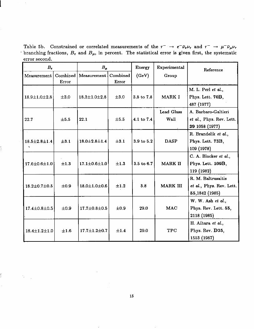
Table 5b. Constrained or correlated measurements of the F --) e-Deu, and F ---) ~-D~u~ * branching fractions, B, and B,, in percent. The statistical error is given first, the systematic

rror second.

& 4 Energy Experimental Reference Measurement Combined Measurement Combined (GeV) Group

Error Error

M. L. Per1 et al.,

18.9fl.Of2.8 f3.0 18.3fl.Of2.8 f3.0 3.8 to 7.8 MARK I Phys. Lett. 70B,

487 (1977)

Lead Glass A. Barbaro-Galtieri

22.7 f5.5 22.1 f5.5 4.1 to 7.4 Wall et al., Phys. Rev. Lett.

39 1058 (1977)

R. Brandelik et al.,

18.5f2.8f1.4 f3.1 18.0f2.8f1.4 f3.1 3.9 to 5.2 DASP Phys. Lett. 73B, .

109 (1978)

C. A. Blocker et al.,

17.6f0.6fl.O f1.3 17.lf0.6fl.O f1.3 3.5 to 6.7 MARK II Phys. Lett. 109B,

119 (1982)

R. M. Baltrusaitis

18.2f0.7f0.5 f0.9 18.0fl.Of0.6 f1.2 3.8 MARK III et al., Phys. Rev. Lett.

55,1842 (1985)

W. W. Ash et al.,

17.4f0.8f0.5 f0.9 17.7f0.8f0.5 f0.9 29.0 MAC Phys. Rev. Lett. 55,

2118 (1985)

H. Aihara et al.,

18.4f1.2fl.O f1.6 17.7f1.2f0.7 f1.4 29.0 TPC Phys. Rev. D35,

1553 (1987)

15

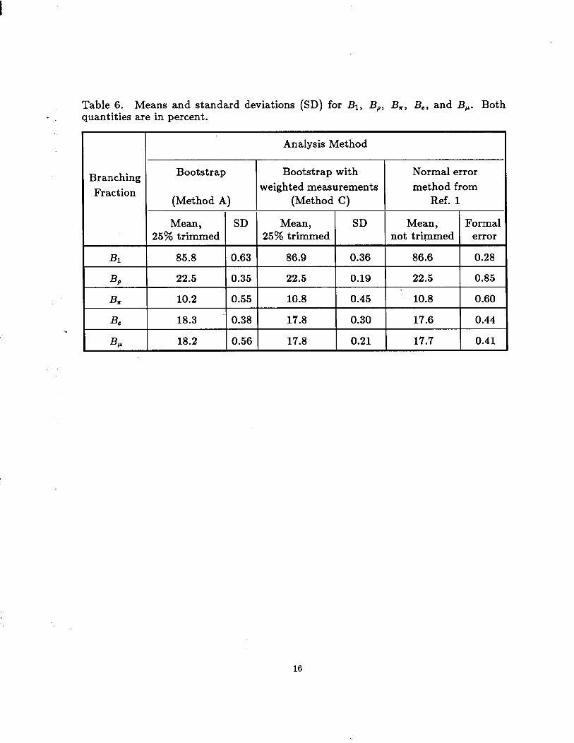
Table 6. Means and standard deviations (SD) for B1, B,, I?,, B,, and B,. Both quantities are in percent.

Analysis Method

Branching Bootstrap Bootstrap with Normal error

Fraction weighted measurements method from (Method A) (Method C) Ref. 1

Mean, SD Mean, SD Mean, Formal 25% trimmed 25% trimmed not trimmed error

Bl 85.8 0.63 86.9 0.36 86.6 0.28

BP 22.5 0.35 22.5 0.19 22.5 0.85

' &i 10.2 0.55 10.8 0.45 10.8 0.60

Bt? 18.3 0.38 17.8 0.30 17.6 0.44

BP 18.2 0.56 17.8 0.21 17.7 0.41

16

Table 7. The 25% trimmed mean and bootstrap confidence levels for AB in percent.

Analysis Method Properties I

of Bootstrap, ignore Bootstrap, use Bootstrap

AB B, - B, correlations B, - B, correlations with weighted

in Table 5b in Table 5b measurements

mean 16.62 16.58 18.01

.Ol confidence

level

.05

confidence

level

.50 confidence

level

.95 confidence

level

.99 confidence

level

14.12 13.94 15.83

14.96 14.86 16.52

16.79 16.87 17.86

18.59 18.70 18.95

19.41 19.43 19.28

17