Embed Size (px)
Citation preview
APPLICATION OF SOFTWARE QUALITY METRICS TO A RELATIONAL DATA BASE SYSTEM
by
Geereddy R. Reddy
Thesis submitted to the Faculty of the
Virginia Polytechnic Institute and State University
in partial fulfillment of the requirements for the degree of
MASTER OF SCIENCE
in
Computer Science
APPROVED:
Dr.:::::t{afura, D,eimis Chairman
Dr. Chachra, Vinod "f>r. Haft'son, Rex
br."""fi'e'nry, Sallie
May, 1984 Blacksburg, Virginia
APPLICATION OF SOFTWARE QUALITY METRICS
TO A RELATIONAL DATA BASE SYSTEM
by
Geereddy R. Reddy
ABSTRACT
It is well known that the cost of large-scale software
systems has become unacceptably high. Software metrics by
giving a quantitative view of software and its development
would prove invaluable to both software designers and
project managers. Although several software quality metrics
have been developed to assess the psychological complexity
of programming tasks, many of these metrics were not
validated on any software system of significant size.
This thesis reports on an effort to validate seven
different software quality metrics on a medium size data
base system. Three different versions of the data base
system that evolved over a period of three years were
analyzed in this study. A redesign of the data base system,
while still in its design phase was also analyzed.
The results indicate the power of software metrics in
identifying the high complexity modules in the system and
also improper integration of enhancements made to an
existing system. The complexity values of the system
components as indicated by the metrics, conform well to an
intuitive understanding of the system by people familiar
with the system. An analysis of the redesigned version of
the data base system showed the usefulness of software
metrics in the design phase by revealing a poorly structured
component of the system.

ACKNOWLEDGMENTS
I wish to express my deep gratitude to Dr. Dennis Kafura,
without whose patient guidance and invaluable technical
advice this work would not have been possible.
discussions with Dr. Sallie Henry are
Illuminating
gratefully
acknowledged. I would like to thank Dr. Vinod Chachra and
Dr. Rex Hartson for serving on my committee and also for
being a constant source of encouragement. I am extremely
grateful to Mr. Bob Larson and Mr. James Canning whose help
and encouragement throughout this work was invaluable.
iv
TABLE OF CONTENTS
ACKNOWLEDGMENTS . . . . . . . . . . . . . . . . . . . . . iv
Chapter
I.
I I.
INTRODUCTION
Motivation for this study Problem statement and Outline Thesis Organization
SURVEY AND DESCRIPTION OF METRICS USED
Introduction . . . . . . . . . Micro Metrics . . . . . . . .
McCabe's Cyclomatic Complexity Halstead's Effort Metric E
Macro Metrics . . . . . . . . . . Henry and Kafura's Information Flow Metric McClure's Control Variable Complexity ... Woodfield's Syntactic Interconnection Model Yau and Collofello's Logical Stability
Measure .
1
1 4 6
7
7 8 8
. 10 13 13 17 20
24
III. IMPLEMENTATION OF THE METRICS 27
IV.
v.
Introduction . 27 Intermediate Files 28
McClure's Control Flow Complexity 31 Woodfield's Syntactic Interconnection Measure 32 Yau and Collofello's Logical Stability Metric 33
MINI DATA BASE -- HISTORY AND HOW IT WORKS
Introduction . . . . An Overview . . .
Basic Structures MDB modules by function
Survey of Different Versions
RESULTS AND DISCUSSION
Correlation Results Closer Look At Outliers Comparison Of Three Versions
Complexity Change -- System Level
v
35
35 37 37 45 49
51
53 55 60 61

VI.
Complexity Change -- Procedure Level Analysis Of New MDB
CONCLUSIONS
65 72
74
REFERENCES . . . . . . . . . . . . . . . . . . . . . . . 86
VITA 89
vi
LIST OF TABLES
Table ~
1. Correlation values Micro Vs. Micro 77
2. Correlation values Micro Vs. Macro 78
3. Correlation values Macro Vs. Macro 79
4. Version 1 High Complexity Outliers 80
5. Version 1 Low Complexity Outliers 81
6. Version 1 Metric Values Statistics 82
7. Percent Complexity Increase Version 1 to Version 2 83
8. Percent Complexity Increase Version 2 to Version 3 84
9. New MDB High Complexity Outliers . . . . 85
vii
LIST OF FIGURES
Figure ~
1. Maintenance Costs vs. Time 3
2. An example of two code segments which both 18
3. Software metrics analyzer 29
4. Tuple Storage Area Page 42
5. System level complexity increase for Micro metrics 62
6. System level complexity increase for Information flow 63
7. System level complexity increase for Macro metrics 64
8. Lexical analysis in Version 1 MDB 68
9. Lexical analysis in Version 2 MDB 69
viii
Chapter I
INTRODUCTION
1.1 MOTIVATION FOR THIS STUDY
An important concern for software scientists today is the
rising costs of developing and maintaining software. As a
result, increasing importance is being attached to the idea
of measuring software characteristics [ Boeh76]. It is only
by such a process of measurement that it will be possible to
determine whether new programming techniques· are having the
desired effect on reducing the problems of software
production.
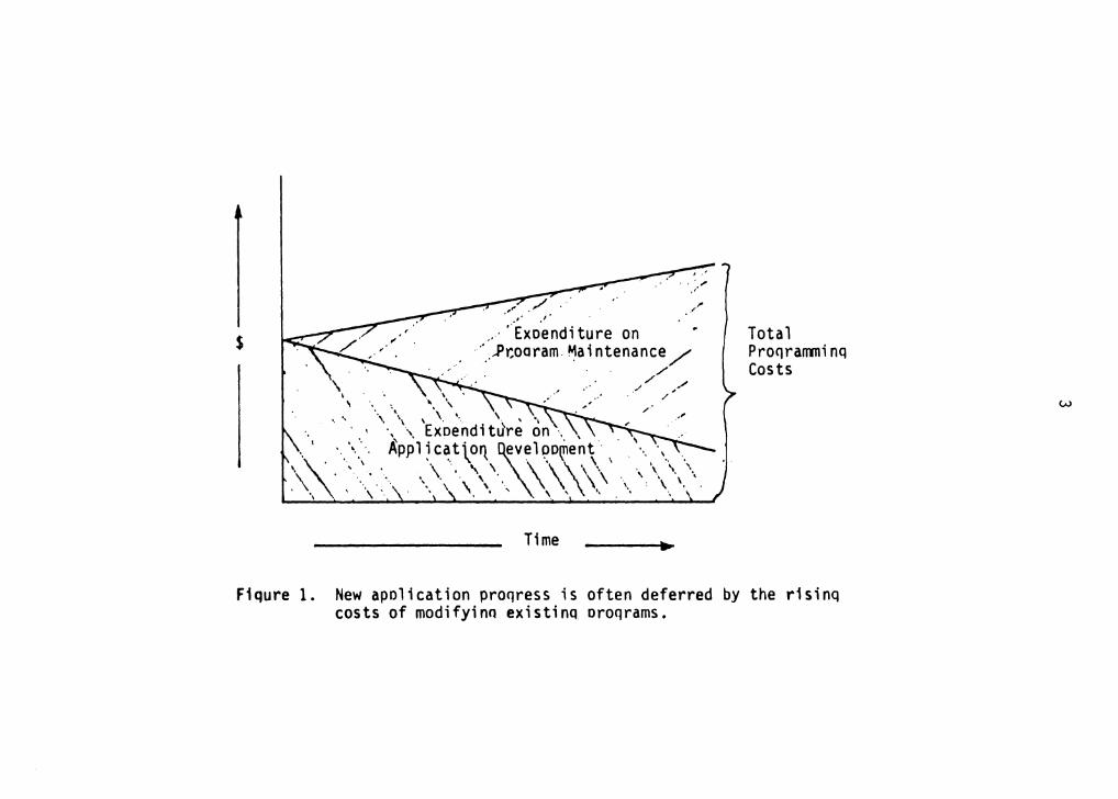
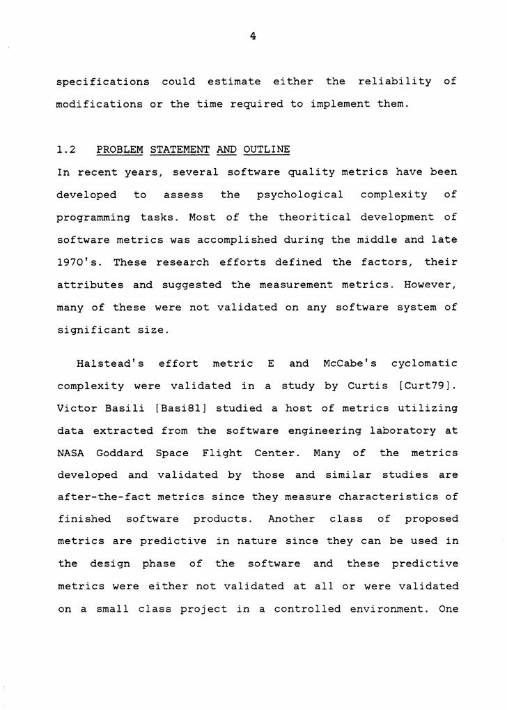
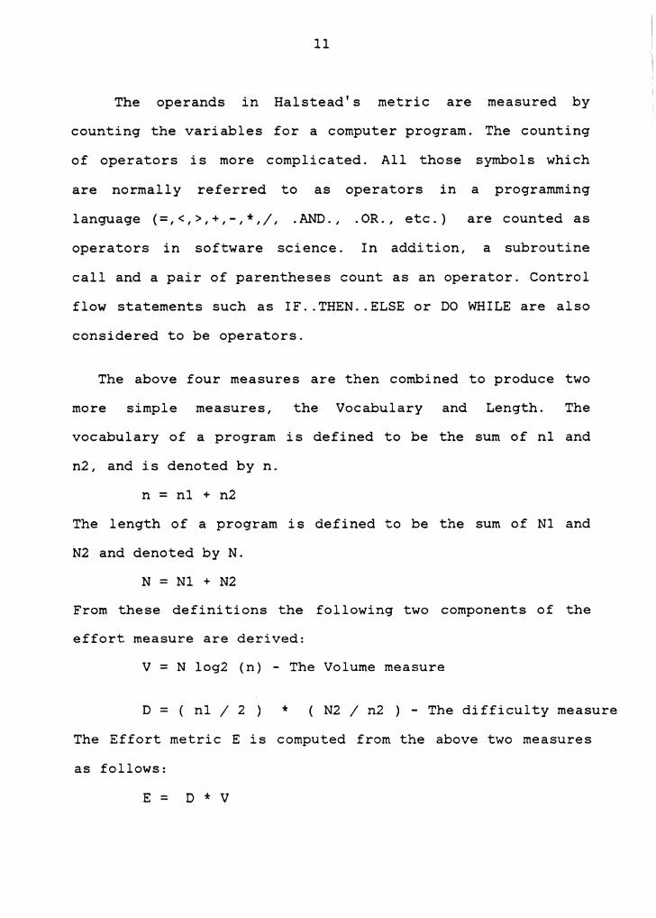
Currently, the software maintenance costs outweigh the
development costs [Boeh79] of a typical large software
system over its life cycle. Also, maintenance costs for a
typical organization take a greater share of the total
software budget than the development costs with an increase
in time as shown in Figure 1 [Mart80]. This figure
highlights the fact that development costs are often
transferred to the maintenance phase of the software life
cycle because of lack of systematic techniques to monitor
the system design. Also, the increased expenditure on
software maintenance leaves diminished resources to be
1

2
allocated for enhancement of this system or new development
of other systems.
The computer industry is thus searching for ways to
produce reliable software and to reduce the cost of software
maintenance. System design techniques have received acclaim
as one answer to this search. Examples of such methodologies
are Composite Design [Myer75] and Structured Analysis Design
Techniques [Ross77]. These methodologies provide a step by
step procedure which guides the system designer. However,
these systematic approaches do not serve as measures of the
quality of design. At best, the designer makes a
qualitative assesment of how judiciously the technique has
been applied. Given the size and complexity of large scale
software systems, the decision process needs to be augmented
by quantitative indicators.
A software metric is a "Measure of the extent or degree
to which a product possesses and exhibits a certain quality,
property or attribute" [Cook82]. Since these metrics give a
quantitative view of software and its development, they
would prove invaluable to software managers who must
allocate the time and resources necessary for software
maintenance and development. For example, Software quality
metrics computed from the complete source code or the design
$
, ... / • 1• I'
,... ···Exo.endi tu re on .1·"
··_ . ..Pr,oaram. ,.,aintenance /
' . . .. ...._ \
/ / / / , ,, /
.-' •. .. .\ '\ ' \ '·.. \. \ ., . • -. \ Exoendi tu're on ·. , . .. . ··.\> /\ppl ~.c~ .. t\o'l ~v~l ~o~· e. "\·., '
\ \· '. . . \ . \ \ \\ . \ . \ ..... ·.. \ \ .\ \ . \ \ \ . . \ ·. \ . . ' . . ' ' ' '• .. \ . . \ . .
Time
Total Proqra1T1T1inq Costs
Fiqure 1. New apolication proqress is often deferred by the r1sinq costs of modifyino existinq oroqrams.
w
4
specifications could estimate either the reliability of
modifications or the time required to implement them.
1.2 PROBLEM STATEMENT AND OUTLINE
In recent years, several software quality metrics have been
developed to assess the psychological complexity of
programming tasks. Most of the theori tic al development of
software metrics was accomplished during the middle and late
1970' s. These research efforts defined the factors, their
attributes and suggested the measurement metrics. However,
~any of these were not validated on any software system of
significant size.
Halstead's effort metric E and McCabe's cyclomatic
complexity were validated in a study by Curtis [Curt79].
Victor Basili [ Basi81] studied a host of metrics utilizing
data extracted from the software engineering laboratory at
NASA Goddard Space Flight Center. Many of the metrics
developed and validated by those and similar studies are
after-the-fact metrics since they measure characteristics of
finished software products. Another class of proposed
metrics are predictive in nature since they can be used in
the design phase of the software and these predictive
metrics were either not validated at all or were validated
on a small class project in a controlled environment. One
5
notable exception to this was the work by Henry and Kafura
[Kafu81a] who suggested a metric based on information flow
and also validated it on the UNIX operating system.
The purpose of this study is to develop an automated tool
for measurement of software quality metrics and to validate
the metrics on a medium size data base management system.
There are seven different metrics generated by this
automated analyzer. These metrics are:
1. McCabe's Cyclomatic complexity number.
2. Halstead's Effort metric E.
3. Lines of code.
4. Henry and Kafura's Information Flow Metric.
5. McClure's Control Flow Metric.
6. Woodfield's Syntactic Interconnection Measure.
7. Yau and Collofello's Logical Stability Metric.
The analyzer was obtained by enhancing an information
flow analyzer already developed at the
Wisconsin at Lacrosse under the direction
University of
of Dr. Sallie
Henry. The information flow analyzer performs a lexical
analysis of FORTRAN source programs and generates the first
four metrics listed above. Thus, the analyzer was modified
to incorporate the remaining three metrics mentioned above.

6
The data base management system examined in this study is
called the Mini Data Base (hereafter referred to as MDB) and
it is based on a relational model and it runs under the VMS
operating system on a VAX 11/780. The MDB is a medium size
software system (16,000 lines of code) developed by graduate
students of the Computer Science Department at Virginia Tech
over the last 7 years. The author himself worked with it in
different roles and is quite familiar with its design and
implementation.
1.3 THESIS ORGANIZATION
This thesis is organized into six chapters. The next chapter
explains the different psychological complexity metrics used
in this study. Chapter three describes the implementation of
the metrics that were automated as a part of the author's
project. This chapter gives an overview of the algorithms
used for these metrics, but does not dwell deeply on the
implementation details. The interested reader may refer to
the external documentation [Anadoc] on the analyzer for more
information. Chapter four gives a brief history of the MDB
and it also includes a discussion of the different versions
of the MDB. Chapter five reports all the results obtained
using tables and plots. Chapter six includes a discussion of
the conclusions that can be drawn from this study and
possible spinoffs from this research.
Chapter II
SURVEY AND DESCRIPTION OF METRICS USED
2.1 INTRODUCTION
This chapter discusses the different complexity measures
that were used in analyzing the Mini Data Base. The nature
of the complexity metrics which are currently being proposed
covers a broad spectrum. Many of these metrics can be
divided into two categories, Micro and Macro. The micro
metrics focus on the individual system components
(procedures and modules) and require a detailed knowledge of
their internal mechanisms. Examples of this category are
Mccabe' s cyclomatic complexity metric and Halstead' s
software science measurements. Macro metrics on the other
hand view the product as a component of a larger system and
consider the interconnections of the system components.
Examples of these metrics are Henry and Kafura's Information
flow metric [Kafu81a] and McClure's control flow metric
[Mccl78]. Each of the complexity measures discussed in this
chapter falls into one of the two categories mentioned above
and is described in the corresponding section.
7
8
2.2 MICRO METRICS
2.2.1 McCabe's Cyclomatic Complexity
McCabe developed the cyclomatic number as a measure of
complexity based upon an analysis of a program control flow
graph. Fundamental to the metric is an interpretation of a
program as a set of strongly connected directed graphs.
Each graph of the cluster represents a flow of control
within a given procedure. Each node in a graph corresponds
to a block of code in the procedure where the flow is
sequential and an arc connecting two nodes corresponds to a
branch taken in the procedure. An additional arc from the
graph's unique exit node to its unique entry node is drawn
to fulfill the strongly connected criteria.
McCabe derived his measure from the cyclomatic number of
a graph as discussed in graph theory. A result from graph
theory states that, in a strongly connected graph G, the
cyclomatic number is equal to the maximum number of linearly
independent circuits. A linearly independent circuit is a
basic path through a graph such that if one has the set of
all possible linearly independent circuits for a given
graph, all possible paths through that graph may be built
out of these circuits. The cyclomatic complexity, V(G}, for

9
the modified graph (with the extra arc added from the exit
node to the entry node) is :
V(G) = E N + 2
where E is the number of edges in the graph and
N is the number of nodes in the graph.
This complexity measure is designed to conform to our
intuitive notion of complexity with regard to a procedure's
testability since the problem of testing all control paths
through a procedure is associated with the problem of
testing all linearly independent circuits.
McCabe used results from Mills [Mill72] to prove that the
cyclomatic complexity V(G) of any structured program can be
expressed as :
V(G) = P + 1
Where P is the number of simple predicates in the program.
One of the reasons McCabe's measure has attracted much
attention may be the ease with which it is calculated.
McCabe validated his metric by testing it in an operational
environment. He cites a close correlation between an
objective complexity ranking of 24 in-house procedures and a
corresponding subjective reliability ranking by project
members [McCa76].

10
Several modifications or enhancements to the McCabe
measure have been
suggested by Myers
proposed. One such enhancement was
[Myer77]. He addressed the question of
how to evaluate the complexity of an IF statement containing
more than one predicate. He defined an interval measure of
complexity (L, U). The upper bound U, represents McCabe's
cyclomatic complexity and the lower bound L, is defined to
be the number of conditional statements plus one.
2.2.2 Halstead's Effort Metric E
Halstead's software science is based upon the premise that
algorithms have measurable characteristics which are
interrelated through laws analogous to physical laws. The
software science effort measure, E, is based on a model of
programming which depends on the following definitions
nl - Number of unique operators in the program
n2 - Number of unique operands in the program
Nl - Total number of occurences of all operators
in the program
N2 - Total number of occurences of all operands
in the program
11
The operands in Halstead's metric are measured by
counting the variables for a computer program. The counting
of operators is more complicated. All those symbols which
are normally ref erred to as operators in a programming
language ( =, <, >, +, - , *, /, . AND., . OR. , etc. ) are counted as
operators in software science. In addition, a subroutine
call and a pair of parentheses count as an operator. Control
flow statements such as IF .. THEN .. ELSE or DO WHILE are also
considered to be operators.
The above four measures are then combined to produce two
more simple measures, the Vocabulary and Length. The
vocabulary of a program is defined to be the sum of nl and
n2, and is denoted by n.
n = nl + n2
The length of a program is defined to be the sum of Nl and
N2 and denoted by N.
N = Nl + N2
From these definitions the following two components of the
effort measure are derived:
V = N log2 (n) - The Volume measure
D = ( nl / 2 ) * ( N2 / n2 ) - The difficulty measure
The Effort metric E is computed from the above two measures
as follows:
E = D * V

12
where the uni ts of E are claimed to be elementary mental
discriminations.
There are two interpretations for Halstead's volume
measure V. The first suggests that the size measure should
reflect the minimum number of bi ts necessary to represent
each of the operators and operands. The second
interpretation assumes that the programmer makes a binary
search through the vocabulary each time an element in the
program is chosen, thus implying that volume may be thought
of as the number of mental comparisons required to generate
a program.
The difficulty measure D implies that program difficulty
level will increase with both an increasing number of unique
operators and an increasing number of recurrent uses of
operands. The constant 2 in the denominator represents the
number of operators needed when a program is written in its
most abstract form - one to perform the algorithm and one to
assign the results to some location.
If we assume that D converts mental steps to elementary
mental discriminations (EMD's), then all we need to know is
the number of EMD's per second, to allow us to convert E to
time. Fitzimmons and Love [Fitz78] have shown that 18 is a
reasonable conversion factor and this was also a number in
13
the range indicated by psychologist John Stroud in his work
[ Stro56] . Halstead used this value to derive the estimated
time T for creating or understanding a program:
T (sec} = E / 18
Although a value of 18 chosen for the EMD's per second
in the above formula gave good results during
experimentation in few studies, it has been a source.of much
controversy. This number has not been generally accepted
among psychologists and Curtis [curt80] states, "Computer
scientists would do well to immediately purge from their
memory the Stroud number of 18 .mental discriminations per
second". Other recent critical evaluation of both the theory
and experimental basis of software science can be found in
[Hame81] and [Otte81].
2.3 MACRO METRICS
2.3.1 Henry and Kafura's Information Flow Metric
Henry and Kafura defined and validated a metric based on
the measurement of information flow between system
components. The information flow measurement permits
evaluation of the complexities of modules within the system
and the complexities of the interfaces between the various
components of the system.

14
There are three types of information flow in a program,
as presented in this study Global flows, Direct local
flows and Indirect local flows. There is a global flow of
information from module A to module B through a global data
structure D, if A deposits information in D and B retrieves
information from D. A direct local flow of information from
module A to module B exists if A calls B. An indirect local
flow of information from A to B exists if either of the
following two conditions is satisfied
i) B calls A and A returns a value to B, which B
subsequently utilizes.
ii) If C calls both A and B passing an output value
from A to B.
One useful property of the information flows defined
above is that, the knowledge necessary to construct the
complete flows structure can be obtained from a simple
procedure by procedure analysis.
An information flow analysis of a system is performed in
three phases. The first involves generating a set of
relations indicating the flow of information through input
parameters, output parameters, returned function values and
global variables. The second phase generates an information
flow structure from these relations. The third phase

15
analyzes the information flow structure to determine the
local and global flows. For a detailed explanation of the
format of relations and the derivation of flows from the
information flow structure, refer to [Henr79].
The procedure complexity as derived by the authors is a
function of two factors the complexity of the procedure
code and the complexity of the procedure's connections to
its environment. The lines of code measure was used for the
internal complexity of the procedure. Fundamental to the
derivation of procedure's interconnection complexity is the
definition of two terms : Fan-in and Fan-out of a procedure.
The Fan-in of a procedure A is the number of local flows
into procedure A plus the number of data structures from
which procedure A retrieves information. The Fan-out of a
procedure A is the number of local flows from procedure A
plus the number of data structures which procedure A
updates. The formula defining the complexity value of a
procedure is :
Procedure complexity = Length * ( Fan-in * Fan-out ) ** 2.
The term fan-in * fan-out represent the total number of
input-output combinations for the procedure. The information
flow term is squared since it is felt that the severity of
problems typically encountered when additional connections

are added
non-linear
product.
between
way with
16
system
respect
components increases
to the fan-in and
in a
fan-out
One attractive feature of this metric is that the major
elements in the information flow analysis can be directly
applied at design time. The availability of a quantitative
measure at such an early stage of the system development
allows restructuring of the system at a low cost.
The authors also performed a validation study of their
metric. The software system chosen for validation was the
UNIX operating system. The study [Henr79] indicated a
statistical correlation of 0.95 between errors and procedure
complexity. Although similar correlations for McCabe's
metric (0.96) and Halstead's effort metric (0.89) occurred,
it was found that these micro metrics were highly correlated
to each other but only weakly related to the information
flow metric. This result suggested that the information flow
metric measured a dimension of complexity different from the
other two metrics.
17
2.3.2 McClure's Control Variable Complexity
McClure's metric focuses on the complexity associated with
the control structures and variables used to direct
procedure invocation in a program. McClure also argues that
all the predicates used in McCabe's measure do not really
contribute the same complexity and thus it is important to
recognize the complexity associated with each of those
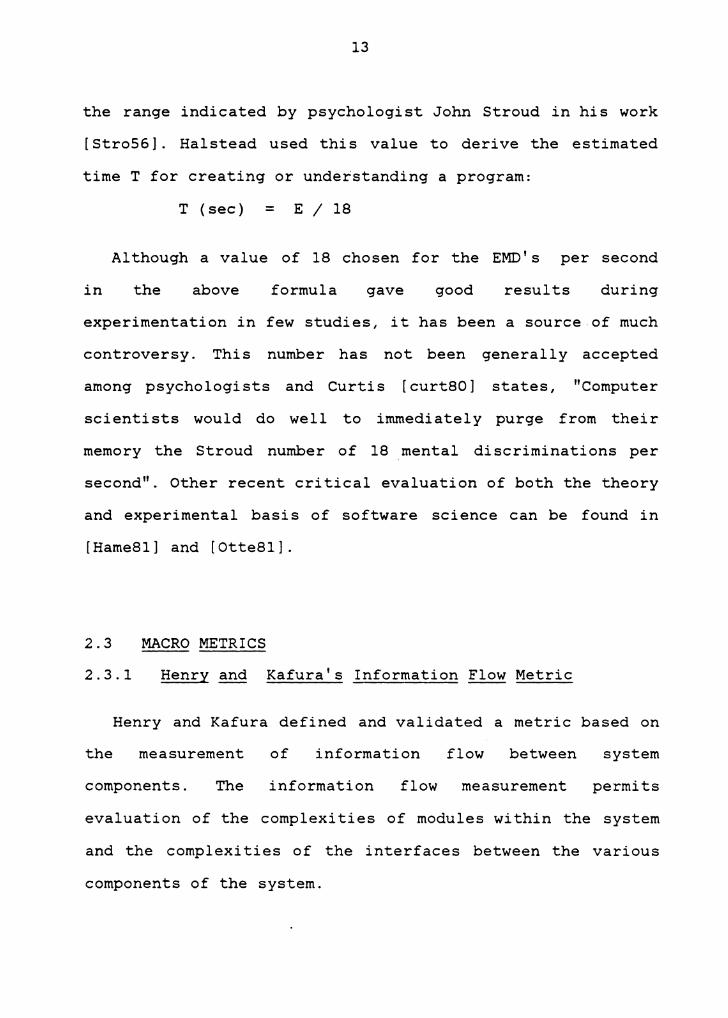
program variables. To illustrate her point, she provides the
example given in Figure 2. Both the modules, A and B have a
McCabe complexity of 6. Intuitively, however she asserts
that module B should have a greater complexity than module
A, because understanding module B requires knowledge of the
possible values of five program variables whereas,
understanding module A requires the knowledge of only one
program variable.
The complexity associated with a control variable is an
important consideration in the derivation of McClure's
program complexity measure. She defines a control variable
as a program variable whose value is used to direct program
path selection. The complexity of a program module P
consists of two factors: first, the complexity associated
with invoking module P and second, the complexity associated
with module P invoking other modules. Both these
complexities are in turn a function of the associated
18
IF tcode = 1 INVOKE add
ELSE IF tcode = 2 INVOKE delete
ELSE IF tcode = 3 INVOKE modifyl
ELSE IF tcode = 4 INVOKE modify2
ELSE IF tcode = 7 INVOKE insert
ELSE error <- 1.
(a) Code for module A
IF tcode = 1 AND name = BLANKS INVOKE create
ELSE IF type = 2 INVOKE modify WHILE filend = 1
ELSE IF cfield = blanks error <- 2
ELSE error <- 3.
(b) Code for module B.
Figure 2: An example of two code segments which both have a cyclomatic number of 6 [McC178].
19
control variable sets. A control variable set is defined as
the set of control variables upon whose value a module
invocation depends. For example, the set {tcode, name } form
a control variable set for invoking module CREATE in module
B. A module may have multiple invocation control variable
sets when it is conditionally invoked in more than one place
in the program.
Using the above concepts,
is calculated for each of
method:
a metric of module complexity
the modules by the following
M ( P ) = ( Fp * X ( p ) ) + ( Gp * Y ( p ) )
where,
Fp is the number of modules which call P.
Gp is the number of modules called by P.
X(p) is the average complexity of all
control variable sets used to invoke P.
Y(p) is the average complexity of all
control variable sets used by module
P to invoke other modules.
The derivation for calculating X(p) and Y(p) are
discussed by McClure in her paper [McC178] and I have chosen
for reasons of brevity not to describe them here.
20
The overall complexity is
the complexities of the
calculated by adding together
modules. McClure makes two
recommendations with respect to the complexity of a
partitioning scheme: the complexity of each module should
be minimized and the complexity among modules should be
evenly distributed.
2.3.3 Woodfield's Syntactic Interconnection Model
Woodfield's comparison of micro metrics lead to the
development of a hybrid model that included the module
interconnections. He found that the software science effort
measure when combined with a model of programming based on
logical modules and the module interconnections produced the
closest estimates to actual programming times [Wood80].
Woodfield's model is based on the premise that it may be
necessary to
understanding
review
the
certain modules
program due
more than once while
to the module
interconnections. He defines the connection relationship as
a partial ordering represented by "->" such that A -> B
implies that one must fully understand the function of
module B before one can understand module A.
21
Module connections are further classified into two types
in the Syntactic Interconnection model : Control and Data.
A control connection A ->c B, exists when some module A
invokes another module B. It is possible that a functional
module may be referenced by several modules in a program,
and therefore needs to be reviewed more than once.
To formally define the conditions under which A is data
connected to B, the following definition of a "data path
set" is needed.
A data path set OBA is defined to be an ordered set of
one or more modules { d 1 , d 2 , d3 , dn } such that one of
the following three conditions is true.
3. There exists some di in OBA such that di calls both
d. 1 and d.+ 1 ; d. 1 calls d. 1 ; d. 2 calls d. 3 ; ... ; i- 1 i- i- i- i-
d2 calls d 1 ; d 1 calls B; Also, di+l calls di+2 ;
di+2 calls di+3 ; ... ; dn-l calls dn; dn calls A.
A data connection A ->d B, exists between two modules A
and B when there is some variable V such that the following
two conditions are true :

22
1. The variable V is modified in B and referenced in A.
2. There exists at least one data path set, DBA' between
B and A such that the same variable V is not referenced
in any di, where di is a member of DBA.
A data path set in the above definition should also
contain at least one member as there is an implicit
assumption that data connections between parent and child
are accounted for by control connections. Condition 2 for a
data connection was included to account for the following
case. Suppose V is referenced in A, B and Q and also
suppose that Q is an element of all data path sets between B
and A. It is then assumed that no extra effort is needed to
understand how the modification of V in B affects the use of
V in A since the effort has already been extended to
comprehend the effect of modified V on Q.
Both the type of connections A ->c B and A ->d B imply
that some aspect of module B must be understood in order to
completely understand module A. The number of times that a
module needs to be reviewed is defined as the Fan-in. It is
assumed that for every instance in which the module is
reviewed, understanding the module becomes easier. Woodfield
thus used a review constant in his derivation of the
23
complexity measure. The module complexity he derived is also
a function of the module's internal complexity and is as
follows:
Complexity = of module A
Internal complexity of module A
Fan-in I k = 1
Review k-l constant
The specific hybrid model developed by Woodfield and used by
the author in his study is referred to as the "Syntactic
Interconnection Model". This model utilizes a review
constant of 2/3, which is a number previously suggested by
Halstead [Hals77]. Woodfield used the software science
effort metric E for the internal complexity of a module.
Woodfield validated his metric on data collected from
student programmers developing programs for a programming
competition. There were thirty small programs ( 18 196
lines of code) and the time needed to complete each program
was compared with results obtained by using the Syntactic -interconnection model. Results indicated that the model was
able to account for 80 percent of the variance in
programming time with an average relative error of only 1
percent.

24
2.3.4 Yau and Collofello's Logical Stability Measure
Yau and Collofello present a measure for estimating the
Stability of a program [Yau80], which is the quality
attribute indicating the resistance to the potential ripple
effect observed when a program is modified. This measure is
developed in an effort to measure the maintainability
characteristics of a software. Since it is not possible to
develop a stability measure based upon probabilities of what
the maintenance effort will consist of, a primitive subset
of the maintenance activity is utilized in measuring the
stability of a program. This consists of a change to a
single variable definition in a module. The authors justify
this by saying that regardless of the complexity of the
maintenance activity, it basically consists of modifications
to variables in the modules.
The procedure consists of first identifying two sets of
variables for each module Vk, set of all variable
definitions in module K, and Tk, the set of all interface
variables in module K. Interface variables are those
variables through which a change may propagate to other
modules. For a module K, this consists of all global
variables in K, input parameters to modules called by module
K and the output parameters of module K.

25
For each variable i in the set Vk' a set Zki is computed.
This set consists of all interface variables in Tk which are
affected by a modification to variable definition i of
module K by intramodule change propagation. Also computed
for each interface variable j of is a
consisting of those modules which are affected by a change
to interface variable j. Thus for each variable definition i
in module K, a set of all modules affected as a consequence
of modifying i, called Wki can be computed.
= u xkj
j £ 2ki
Yau and Collofello then used the McCabe complexity of each
module in the set Wki and summed it to form the logical
complexity of modification of variable i in module K
represented as LCMki"
LCMki = !
t £ wki
where, ct is the cyclomatic complexity of module t.
The authors then define the ripple effect for module K
(LREk) to be the mean LCMki for all variable definitions in
module K.
= !
i £ vk where, Nk is the number of variables in module k.
The logical ripple effect in the above equation represents a
measure of the expected impact on the system, of a

26
modification to a variable in module K. A measure for the
stability of a module K, denoted as LSk is established as :
LSk = 1 / LREk.
An important requirement of the stability measures
necessary to increase their applicability and acceptance is
the capability to validate them. The authors claim that
their measure is more easily automatable than previously
suggested measures and thus easily lends itself to
validation studies. They also chose to validate the metrics
indirectly by a logical argument that this measure
incorporates and reflects some aspects of program design
generally recognized as contributing to the development of
program stability during maintenance.
Chapter III
IMPLEMENTATION OF THE METRICS
3.1 INTRODUCTION
To gather the metrics needed for this study, an analyzer
was obtained by enhancing an information flow analyzer
already developed at the University of Wisconsin at Lacrosse
under the direction of Dr. Sallie Henry. The information
flow analyzer which performs a lexical analysis of FORTRAN
source programs generates all micro metrics, The lines of
code metric, Halstead's software science measure and
McCabe's cyclomatic number apart from computing information
flow complexity. It was thus modified to compute the
remaining three macro metrics used in this study.
This chapter explains only the algorithms used to compute
the different metrics and does not dwell much into the data
structures used and other details. The interested reader
may please refer to the documentation on this analyzer
[Anadoc] for any detailed information.
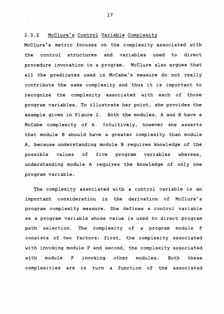
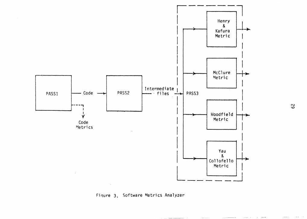
The structure of the analyzer can be best described by
organizing it into three phases as shown in figure 3. PASSl
of the analyzer is essentially a sophisticated lexical
27
28
analyzer and it is completely language dependent. It also
generates the three micro metrics: Halstead's measure,
McCabe's cyclomatic complexity and the lines of code metric.
PASS2 of the analyzer generates several pieces of
information that are later used by each of the macro metric
generators. The output generated by PASS2 is also divided
into different files and the following subsection explains
this information in detai 1. PASS3 of the analyzer can be
further divided into four parallel units as shown in figure
3, where each of the four units generates one of the macro
metrics.
3 .1.1 Intermediate Files
The significant information generated by PASS2 is contained
in the following files: Relation, Localfile, Pcfile and
Invoked.
Relation
The relation file contains the relations used by Henry
and Kafura to generate the information flow metric. In
general, a relation can be represented by :
Destination <-- Sourcel,Source2, ... ,SourceN.
There are four possible
destination i) X.n. I
ways of denoting the source and
denoting the value of nth input
PASSI Code ~
---, I I r
Code ~1etri cs
PASS2 Intermediate
i-- · files
,-----1 I I I
Henry I ~ ' & -,. Kafura r
Metric I I I I
' McClure I ,. I -"'letri c I
PASS3 I I
~/oodfi el d . r
I Metric
I I
Yau I . & I .
Collofello ,.
Metric I L _____ :J Firiure 3. Software ~etrics Analyzer
·N ~
30
parameter of procedure X at the procedure's invocation; ii)
X.n.O denoting the value of the nth parameter of procedure X
at the procedure exit point; iii) If X is a function, X.O
denotes the value returned by that function; and iv) X.D
denotes an access by procedure X to the global data object
D.
For a
relations,
relations
more detailed explanation and examples of
please refer to [Henr79]. Notice that the
as defined above only indicate the flow of
information between the interface variables in the program.
Localfile
The Localfile contains relations that are local to a
procedure. The form used to represent the local relations is
essentially the same as used for the interface relations,
except the source or destination can have one additional
possible form, X.locvar.Z, denoting the local variable
called Z in procedure X. These local relations are required
for computing the Yau and Collofello logical stability
metric, as they identify the ripple caused by the local
variable definitions in a procedure.
Pc file

31
This file contains the calling information in a program.
The notation used to represent a procedure call is
straightforward. Each record in the file represents a call
and it has the called procedure followed by the calling
procedure. This information is used to build a calling graph
which is later used in Woodfield and McClure's metrics.
Invoked
This file is used only by the McClure metric generator.
Its contents are a list of control variable sets found in a
given program. For each control variable set, the names of
the invoking and invoked procedures are provided. A control
variable set is fully described by listing each of the
variables in the set together with each variable weighting
term.
3.2 MCCLURE'S CONTROL FLOW COMPLEXITY
The first major function of the McClure metric analyzer
is to build four fundamental data structures. These
structures (Calling graph, Varinfo tree, Global tree and
Var sets) contain information such as the list of control
variable sets, the calling hierarchy and individual variable
details required in McClure metric computation. After these

32
structures have been built, this implementation of the
McClure metric uses a bottom-up approach to compute
procedure complexity.
First, for each control variable in the program, the IV
and DEGREE weights as described by McClure, are computed.
These weights are then used in the calculation of each
control variable' s complexity. Next, the complexity of a
control variable set is derived by summing the complexity of
its individual control variables. Finally for each procedure
X, McClure's complexity value is obtained by utilizing the
complexity of all control variable sets which cause control
to flow either from procedure X, or to procedure X.
3.3 WOODFIELD'S SYNTACTIC INTERCONNECTION MEASURE
As you may recall, Woodfield's syntactic interconnection
measure consists of two components control connections
and data connections. Both of these connections require the
procedure calling information, and to allow for that the
first step used in this algorithm consists of building a
calling graph. This graph is built using the Pcfile
generated by PASS2.

33
In the second step, for each global data structure, DS,
in the program, nodes in the calling graph are marked to
indicate whether the procedure references or modifies the
data structure. After each marking, a procedure for finding
all the data connections from this marked calling graph is
invoked. The information used to mark the graph is obtained
from the Relation file.
The third step consists of finding all the control
connections from the graph. This is straightforward once we
have the calling graph.
The last step involves computing the Woodfield fanin for
each procedure from the information derived above, and then
doing the arithmetic neccessary to obtain Woodfield's metric
for each procedure.
3.4 YAU AND COLLOFELLO'S LOGICAL STABILITY METRIC
The following steps describe the algorithm used to compute
the logical stability measure
Step l For each interface variable in the program, identify
the set of variables it flows into directly. This direct
ripple information is obtained from the Relation and
Localfile files.

34
Step 2 For each local variable i in every procedure K,
identify the set Zki of interface variables which are
affected by a modification to variable definition i by
change propagation within the procedure. This information is
directly read from the Localfile generated by PASS2.
Step ~ For each interface variable in Zki generated above,
the set Wki consisting of the set of modules involved in
intermodule change propagation is generated by using the
ripple for interface variables generated in step 1. The
program used to compute this set Wki is recursively setup to
generate the ripple effect to any number of levels as
desired, al though a propagation level of 1 was used in
reporting the results of this study.
Step 4 All the arithmetic neccessary to compute the
stability measure from the information obtained in the above
steps is done here.
Chapter IV
MINI DATA BASE -- HISTORY AND HOW IT WORKS
4.1 INTRODUCTION
MDB is a database management system based on the relational
model and running on a DEC VAXll/780 under the VMS operating
system. The MDB system is written in FORTRAN and supports
only a single user. Each user process has a complete copy of
the MDB executable code and has exclusive use of one
database file at the time it is in use. The MDB provides a
variety of commands which enable users to:
1. Create a database.
2. Define, load, store or drop relations in a database.
3. Load and store tuples into and from a relation.
4. Insert, modify and delete individual tuples in
a relation.
5. Query relations.
6. Rerun commands or use an editor to modify them.
7. Execute files of commands
The original work on MDB started in the spring of 1977 as
a class project in the computer Science Department at
Virginia Tech. A graduate level course in database system
35
36
construction formulated goals and the design details for a
database management system for the LSI-11 microcomputer. A
second database class in the spring of 1978 produced a
working system a limited DBMS using floppy disk storage.
This was based on the original goals of the previous year
and on revisions of that design. Over the next few years,
students worked on parts of the MDB for their masters
projects and the system was moved to the VAX-11/780. In
spring of 1981, a graduate class added a number of
enhancements. The earliest version of the MDB source code
available today is the one produced by the spring 1981 class
and it is the first of the three versions of MDB analyzed in
this study. The three versions chosen by the author for
analysis are the spring 81, spring 82 and spring 83 classes'
final products. These three versions are also referred to as
version l, version 2 and version 3 respectively later in
this thesis.
The following section gives an overview of the MDB. The
last section in this chapter contains a survey of the three
versions mentioned. The discussion of those three versions
is postponed to the last section to give the reader a better
understanding of the enhancements done on each of those
versions.
37
4.2 AN OVERVIEW
4.2.1 Basic Structures
Each database created using the MDB is a sequentially
organized file consisting of fixed length records (pages) of
512 bytes each, residing on a direct access device. Seven
data structures contain most of the information about the
MDB and are stored in the pages of each database file. A
database utilizes directory, index (B-trees) and stored
tuple (user data records), among other things. Understanding
the format of these structures should provide insight into
how the programs that use these structures work and also
make it easier to interpret the results reported in this
study. This subsection of the report is a rewrite of a
chapter from the MDB documentation manual [MDBdoc] for the
most part.
System Pages
The MDB requires that the first two pages of the database
file be allocated for DBMS use.
The first page is the page map. Each of 4096 bits is used
to represent whether a database page has been allocated or
is free. If the bit is set to 1 (on), the page is allocated
to some relation in the database, otherwise the bit is set
toO(off).
38
The second page is used to store the MDB design
parameters. Information such as the length of each entry in
the database system directory (DSD), the maximum length in
words of the DSD, the maximum number of attributes per
relation, and the number of pages in the database are stored
on this page. This page is read by subroutine DBUP at the
start of each database session in order to initialize
variables containing these design parameters.
The Database System Directory (DSD)
The DSD exists in each database, defined within a common
block named DBSD and contains the following information
about each relation therein:
1. The name of the relation.
2. The number of attributes in the relation.
3. The page number of the relation's relation directory.
The Relation Directory (RD)
The RD contains information about a particular relation
in a database. There is a separate two-page long RD for
each relation. RD is defined within a common block, named
RD. This size permits a total of thirty-six attributes for
each relation.
Three kinds of information are contained in RD:
1. The number of tuples in the relation.

39
2. Immediately following is the page number of the tuple
storage area map (A table that provides indirect
addressing to the tuple storage location).
3. The remainder of this directory contains information
about attributes in the relation. For each attribute
this consists of
a) The name of the attribute.
b) The type of the attribute, i.e. whether
it is character or integer.
c) Whether the attribute is indexed or not.
If it is indexed, a pointer to the root of
the B-tree index is stored there.
The Tuple Storage Area Map
The TSAMAP provides an interface between the physical
storage system of the VAX and the database. A certain number
of physical disk pages are required to store the tuples of
each relation, and the TSAMAP for each relation keeps track
of these pages. TSAMAP is two pages long, and uses two words
to store four kinds of information about each physical page
of tuples in the relation:
1. A flag to tell the database whether or not the page is
presently in main memory.
2. The physical address of the page.
3. The number of slots allocated. This provides

40
information about how many more tuples can be
added to the page.
4. The number of free words on the page. This also
provides information on how many additional tuples
can be added to the page.
Tuple Storage and the Tuple ID
As described above, the TSAMAP points to a collection of
physical pages stored on disk. There is a unique address, or
tuple identifier (TID) for each tuple in a relation and a
part of the TID represents indirectly, the page number on
which the tuple resides.
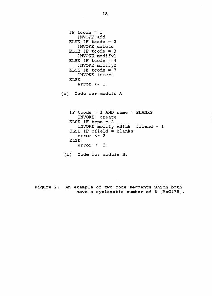
One tuple storage page contains three types of items: the
tuples themselves, the length of each tuple stored on the
page, and a count of the number of active tuples on the
page. The length of each tuple is stored in a slot. The
slots are located at the bottom of the page. Slot number one
is the last word on the page. Slot number two is immediately
above it, and so forth as shown in figure 3. Slot 1 contains
the length of tuple 1, which is not a real tuple but is
always the count of the number of active tuples on the page
excluding itself. Therefore the first tuple always has a
length of one. Slot 2 contains the length of tuple 2 which
is the first real tuple of data. The tuples are entered

41
sequentially from the top of the page. The slots provide a
means of locating any tuple on the page.
B-Trees
Tuples can be located more quickly if attributes are
indexed than if attributes are not indexed, but some
additional time and storage costs are incurred to maintain
two additional structures called the B-tree and the Valtid.
As you may recall, there is an entry in the relation
directory that points to the root of the B-tree if an
attribute is indexed. There is a separate B-tree for every
indexed attribute. If a relation contains no indexed
attribute, then there is no B-tree for that relation.
The B-tree is a balanced tree that contains keys and
pointers. A key is a value in the relation for the indexed
attribute. The keys are ordered alphabetically. After each
key, is a pointer to the Val tid page that contains the
actual TID numbers of those tuples with this key as the
value for the attribute or values that are greater than this
key but not equal to the next key on the B-tree page. By
searching along a chain of these pointers, the Valtid pages
with keys that meet the predicates are found quickly. When
the B-tree page fills up, the page is split in half. This
keeps the B-tree as flat as possible. A flat tree reduces

42
# of tuples on page
Tuple 1
Tuple 2
Slot 64 (length of tuple 63)
Slot 3 (length of tuple 2)
Slot 2 (length of tuple 1)
Slot 1
Figure 4: Tuple Storage Area Page
43
the number of levels to be searched. There is a separate
set of subroutines that are used to maintain these B-trees,
and they are discussed later in this chapter.
The Value/TID Storage Area
The VALTID contains keys as do the B-tree pages, that are
also attribute values. The list of TID' s that have this
value for this attribute follows the key. For example, if
the indexed attribute in a relation is COLOR, the Valtid may
contain an entry RED for a key, followed by a list of TID's
whose tuples, for the attribute COLOR, contain the value
RED. The values (keys) are also ordered alphabetically to
facilitate searching and insertion. The Val tid data
structure is arranged the same way that the tuple storage
area is arranged, with the page divided into slots.
The Page Allocation Table
Most databases are dynamic. As tuples are added and
deleted from relations, storage pages may fill or become
empty. As more relations are added, more relation
directories and TSAMAPs are needed. One final structure is
used to keep track of the number of pages of a database file
that are in use. Currently, up to 4096 physical pages are
available for each database depending on the number of pages
44
specified when the user created the database file. PT (page
table) is used to keep track of these pages, and as
subroutines add or delete pages, PT is updated to reflect
these changes.
The Storage Hierarchy
Hopefully, it should now become evident that the database
uses a hierarchical indexing system to keep track of
relations and tuples. Four levels of indexing define a path
to any tuple in a relation. Given a relation name and an
attribute, a tuple or tuples can be located to match those
specifications by moving from the DSD to the RD, and from
the RD to the TSAMAP. The TSAMAP points directly into the
physical storage pages of the tuples. The slot numbers are
the lowest index level.
The B-tree and Valtid provide a shortcut to finding
tuples by storing the TIDs of certain indexed tuples. Since
the TSAMAP provides the mapping from the page number portion
of the TID to the physical page number, the TID is converted
to the physical address of the tuple by a lookup in the
TSAMAP.
All the subroutines in the database source code execute
to interpret user commands and effect changes to the
45
database by manipulating the information contained in these
structures.
4.2.2 MDB modules ~ function
Following is a classification of the MDB procedures into
modules by the functions they perform :
Initialization/Termination
The five routines
Create
Database
Dbmain
Db up
Dbdown
Opens
create a new database, initialize the state of the database
when a session begins every time, open certain files that
are needed, and terminate a database session by saving
pertinent information and closing files.
User Communications
The routines in this module interact with the user,
prompting for values to be used as input for a command,
46
notifying the user of errors, and obtaining responses from
the user terminal. Due to the large number of people that
have worked on the database over a long period of time,
these communications have been implemented somewhat
haphazardly. Not all communications are confined exclusively
to these routines, but some can be found embedded in various
sundry other sections of code. Some of the routines in this
module are:
Error
Getval
Messg
Prompt
Command Analysis
These routines handle all the parsing and command
analysis. DO LEX performs lexical analysis for most of the
commands, using one large state table. CMANAL and SCHKEY
also assist in the interpretation of user commands and
CMANAL drives DOLEX.
Command Execution
Two routines called PROC and PROCES actually initiate the
tasks required by the user command. PROC contains a section
of code for each type of command.
Data Manipulation Language (DML) Functions:
47
This module interacts with the stored data and with the
data structures that are used to keep track of this data.
Four principal operations can be identified:
1. Inserting tuples into the database.
2. Deleting tuples from the database.
3. Moving tuples around in the database.
4. Searching for specific tuples in the database.
These operations require changes to the B-tree, the DBSD,
the TSA, the TSAMAP, and the RD.
Paging
These routines handle the work of keeping track of page
storage for the database. Database pages are the same size
(512 bytes) as physical VAX. pages.
Access
The subroutines in this module are the ones that handle
all data manipulations dealing with B-Trees. All B-Tree
searching, splitting, and building functions are performed
by this module.
Session Management
This module performs all the session management functions
like counting disk I/O's, counting CPU time on an operation,
48
running DCL commands from MDB etc. Most of these functions
were first implemented in spring 1982 version.
Query Optimization
Database queries are made with the use of predicates, and
the database must be searched to locate a match or matches
for the predicate. A tree structure called the predicate
tree is built to find the optimal method of retrieval of the
tuples. The subroutines in this module are involved in
building and the traversal of this predicate tree.
Service Routines
There are certain processes that need to be executed over
and over, often by different parts of the database code.
These routines provide these functions, particularly table
look-up and certain types of character manipulation that is
not convenient to perform in FORTRAN.
Sorting and Merging
After the MDB retrieves all qualifying tuples for a
query, It is at times very convenient to be able to report
the tuples in a certain order. Thi's requires a set of
routines that could sort tuples and merge lists of tuples.
The subroutines performing these functions makeup this
module.
49
Data Definition Language (DDL) Functions
The subroutines in this module perform all the data
definition functions such as those for defining and creating
schemas, dropping schemas, di splaying schemas etc. These
subroutines interact with the DSD and the RD data
structures.
4.3 SURVEY OF DIFFERENT VERSIONS
Spring 1981 (Version 1)
This is the first of three versions used in this study
and is also the oldest version for which any source code was
available. It has most of the functions described above
except for sorting and merging. Other functions like DDL and
Session management also existed, but to a very limited
extent.
Spring 1982 (Version ~)
Many enhancements were made to the MDB in this version.
Almost all these enhancements consisted of adding new
50
commands and new capabilities to the MDB. Some of the new
features include the capabilities to store and load data,
schema, and command files, to invoke execution of command
files, to modify a previous command using an editor, to run
VAX DCL commands without leaving the MDB environment, to
save all changes to the database automatically or on demand,
and enhance the capabilities of a SELECT command used to
query the database for tuples.
One interesting aspect of the enhancements made in this
release is that 12 new commands were added for which
recognition is done directly in NEXTQB, a subroutine called
by DOLEX to get the next line of user input. Although the
correct place to insert this command recognition would have
been DOLEX.
Spring 1983 (version ~)
Most of the enhancements made in this release are in the
form of bug fixing. The only new feature added is in sorting
and merging function, which was rewritten to a good extent
and also made more powerful. A few cosmetic changes were
also made in displaying the schemas.
Chapter V
RESULTS AND DISCUSSION
Seven different metrics were gathered for each procedure
in each version of the MDB. Also, three of the macro
metrics used Information Flow, Syntactic Interconnection
and Logical Stability were weighted by three different
measures for calculating the procedure code complexity. The
three weighting measures used are Lines of Code metric,
Cyclomatic Complexity and Halstead' s Effort measure. The
macro metrics were weighted by the micro measures because
this was also the approach taken by the original authors of
these metrics in their work. Although the authors for these
metrics used only one micro measure in calculating procedure
code complexity, they suggested that any of the micro
measures could be used for calculating the complexity. An
unweighted macro measure for each of these macro measures
was also generated by using a procedure internal complexity
of 1. Thus, for each procedure, 16 different complexity
numbers were generated (4 each for Information Flow,
Syntactic Interconnection and Logical Stability; 1 each for
Control Flow, Lines of Code, Cyclomatic Complexity and
Halstead' s Effort metric). For reasons of brevity, the
results reported here do not give all the 16 measures for
51

52
each procedure. The tables and plots shown in this chapter
are fairly representative of the general pattern observed in
the results.
The original plan of this thesis was to analyze the three
different versions (spring 1981, spring 1982 and spring
1983) of the MDB source code. During the Fall of 1983, an
advanced graduate class in Information Systems in the
Computer Science Department at Virginia Tech started on a
project to redesign the MDB. That work was followed up by an
other class in Winter 1984 to do more detailed design work
and the required programming for the new MDB. Al though, a
complete source code is not available as yet, the design is
specified to an extent that identifies the different
procedures and their various interconnections. This version
of the MDB, referred to as New MDB later in this thesis was
also analyzed and the results of this study are also
reported in this chapter.
There are two basic approaches to validating software
metrics: One, an empirical or objective evaluation and two,
a subjective evaluation of the complexity values by people
familiar with the system being analyzed. This research
includes both the types of validation although it emphasizes
on subjective evaluation. The empirical validation used in
53
this study consists of analyzing the correlation factors
between the different metrics. A careful manual analysis of
the complexity values generated was done as part of the
subjective evaluation. To substantiate the conclusions
drawn from such an analysis, an evaluation of the results by
people familiar with the MDB is also included in this
report. There were two people who were asked to confirm the
results. One of them, Dr. Rex Hartson, has been the director
of the MDB project since its inception. Since he worked with
all versions of the MDB that evolved over the last 7 years,
he is very familiar with the MDB procedures, functions and
their evolution. The other person, Mr. Bob Larson worked
with all the versions of the MDB analyzed in this study
including the New MDB, in different roles. He is currently
the project administrator for the New MDB project. These
two are easily the two persons most familiar with the MDB
design and implementation.
5.1 CORRELATION RESULTS
One of the things it was hoped this study could show was
the fact that the micro and the macro metrics measure a
different dimension of complexity. Both parametric and
non-parametric correlation factors amongst the different
54
complexity metrics were obtained to study this issue. These
statistics were generated for each of the three versions and
also for all the versions combined. Tables 1-3 show the
correlation factors obtained when all the three versions
were combined. The macro, metrics for which results are
reported in these tables are the unweighted metric values
(Procedure code complexity obtained by using a value of 1
for the internal complexity of the procedures). The author
believes that it is more appropriate to use unweighted macro
measures in the above mentioned tables because, what we are
examining is the similarity between the micro and macro
measures, and such a similarity computation is done
accurately when the macro measures do not already contain a
factor of the micro measures. In any case, the correlation
factors obtained by using the micro metrics for weights are
quite similar to the ones shown in Table 2, except for
Woodfield' s metric. Woodfield' s metric shows a very high
correlation with the micro metrics when weighted by any of
the micro metrics. This can be explained easily by a closer
look at the method used by Woodfield to calculate the
procedure complexity. The factor contributed by the
procedure's interconnections is very small because of the
review factor used in Woodfield's calculation, as compared
to the micro metric weight in the calculation of procedure
complexity.
55
The results obtained show that Lines of Code , Effort,
and Cyclomatic metrics are highly correlated to each other
(in the range of 0.79 to 0.97), whereas none of these micro
metrics correlates well with any of the macro metrics (in
the range of 0.04 to 0.49). This implies that the
distinction made in earlier works between micro and macro
metrics [ Kafu81a] is substantial. It was also found that
the macro metrics had a relatively low correlation amongst
themselves as shown in table 3. This is an interesting
result and tells us that each of the macro metrics measures
a different component of the module interconnections. A
similar result was obtained in a work by Canning [ Cann84]
that concluded recently, in which a large software system
from NASA Goddard Space Flight Center was analyzed.
5.2 CLOSER LOOK AT OUTLIERS
An analysis of the procedures that have a very high or
low complexity is deemed useful for determining how accurate
and useful the complexity measurements are. To study such
outliers, the Spring 1981 version was chosen for analysis
and the results reported in this section. The outliers were
identified by first sorting the procedures by their
complexity value for each of the complexity metrics and then
56
taking the union of those procedures that appeared in the
few most complex and least complex procedures for each of
the complexity metrics.
For the macro metrics:
stability, and Syntactic
Information
interconnection
flow, Logical
measure, the
measures used in the above analysis were the ones weighted
by Lines of code, Cyclomatic complexity and Halstead's
Effort metric respectively. Al though the authors of these
metrics suggested the use of any of the micro measures, the
above micro measures were the ones used by the authors in
their work. Tables 4 and 5 give all the seven complexity
metrics for each of the outliers obtained above. To
interpret the results better, Table 6 is drawn to show the
mean, standard deviation, minimum and the maximum values in
the entire set of Version 1 procedures. These statistics are
also derived for all the seven metrics used to obtain the
outliers.
The results obtained by the above analysis agreed well
with the intuitive understanding of the procedures in the
MDB. This fact has been confirmed in a subjective evaluation
of the MDB.
57
"The complexity measurement results concur completely
with our experience and intuition in identifying those parts
of the MDB which were most bug-ridden,troublesome and
frustrating to the programming teams doing the maintenance
and modification" 1
To gain further insight into how well the metrics
identified the complex procedures, a brief discussion of
some of the procedures in Tables 4 and 5 is given below. One
of the procedures (PROC) which has a very high complexity
measure for most of the metrics is discussed in greater
detail.
PROC
This procedure executes the user commands and is the
highest level procedure in the command execution module. A
detailed analysis of PROC shows that, instead of recognizing
the class of database command (classes include DDL, DML and
Session Management.) and calling an appropriate routine to
perform the corresponding function, PROC has a separate
section for performing the command to a good extent.
Al though there are lower level procedures to perform the
primitives required for each of the database commands, the
1 Comments by Dr. Rex Hartson and Mr. Bob Larson
58
command execution module can be split into 3 different
procedures that perform the corresponding database function:
DDL, DML and Session Management. To give a specific example
of the extensive command execution done by PROC, the command
to UPDATE some tuples in the database is done as follows in
PROC:
1. A procedure (QPROC) is called to retrieve the
qualifying tuples.
2. For each qualifying tuple retrieved, the
procedure (QSELCT) is called to print out
the tuple to user for inspection.
3. PROC calls appropriate User Communications
routines to obtain input from the user, to
find out if the tuple really needs to be
updated or not.
4. If the response is yes, the tuple is updated
in PROC for each tuple. There is also a
dialogue with the user from PROC to find
out if he wants to continue with the
UPDATE function.
In the New MDB designed in Fall 1984, the functions
performed by PROC are not anymore performed in one giant
procedure and are instead divided into different procedures.
This provides an evidence that PROC is considered to be a
59
high stress point in the system and it is well indicated by
the metrics.
CMANAL
This procedure performs the function of command analysis in
the MDB. It is also the main procedure in the Command
analysis module of the MDB, described in chapter 3. It
constitutes about 60% of the total lines of code in the
command analysis module. The high complexity measurements
shown for this procedure agree well with an intuitive
understanding of the procedure's complexity.
MESSG
This procedure is used to print messages to the user and is
called from several places in the MDB. The complexity values
for this procedure confirm the fact that each of the
complexity metrics only measures a different dimension of
complexity. As one can see from Table 4, there is no Logical
Ripple caused by this procedure and it has a very small
cyclomatic complexity, al though all the other metrics are
quite large for this procedure. A close look at the program
logic in MESSG shows that the the procedure has a computed
GOTO statement that determines the message to be printed and
the procedure is really not a bottleneck in the system.
60
This procedure is typical of the type of procedures that
might indicate some high complexity,
point of concern to the designer.
illustrates the advantage in using
measurements instead of relying on
software metrics.
Low Complexity Procedures
but are really not a
The procedure also
different complexity
only a few of the
All the procedures in Table 5 perform an elementary
function and are usually not called by more than one
procedure in the MDB. As a result, The complexity values
they indicate are consistent with an intuitive understanding
of the procedure's complexity values.
5.3 COMPARISON OF THREE VERSIONS
One important part of this validation study is to analyze
the change in the complexity of the MDB from one version to
the next. The comparisons between the 3 versions of the MDB
were made at two different levels of the system : First, the
total complexity of the system for each of the seven metrics
was computed on each version, and these complexity values
compared. Second, the percent change in complexity from one
version to the next,
the results analyzed.
61
for each procedure, was computed and
The following subsections discuss the
results obtained by using the above two approaches.
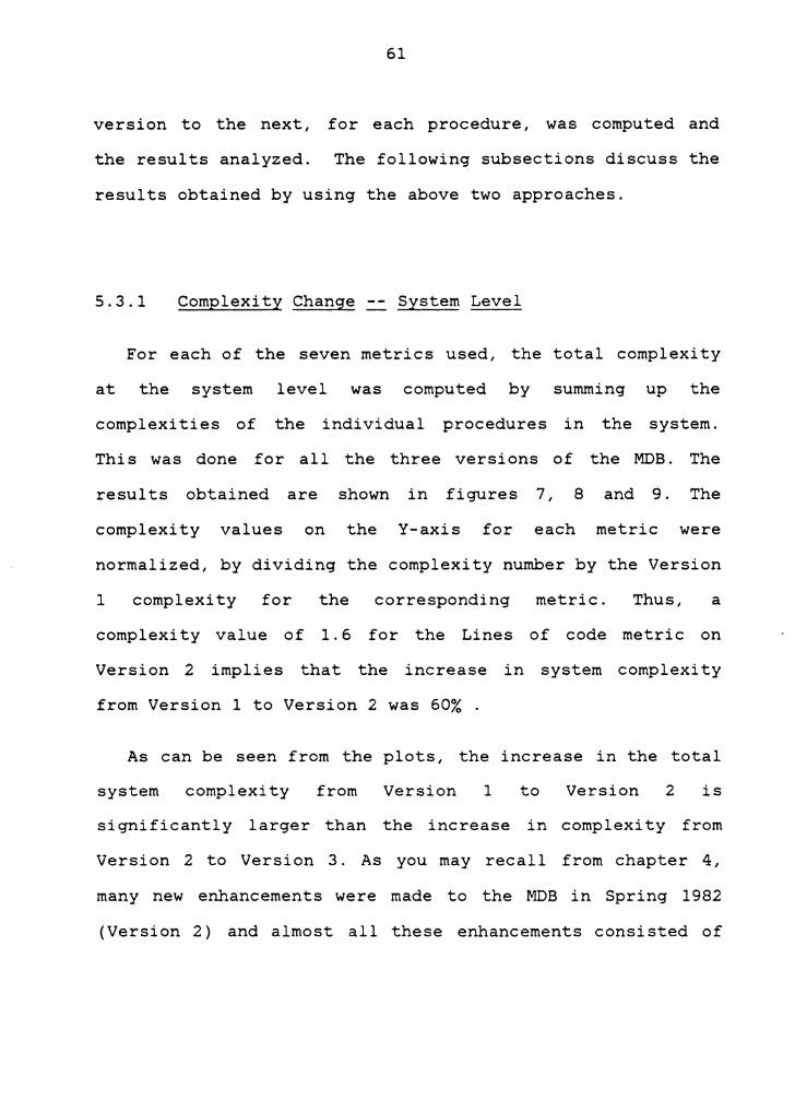
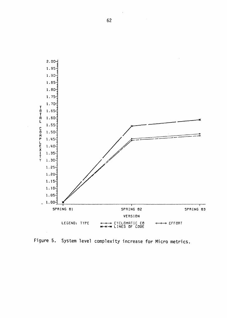
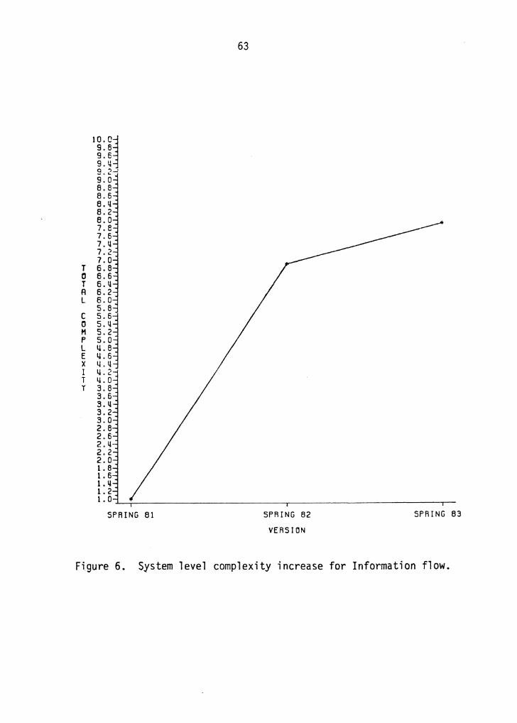
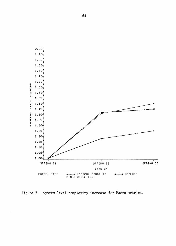
5.3.1 Complexity Change System Level
For each of the seven metrics used, the total complexity
at the system level was computed by summing up the
complexities of the individual procedures in the system.
This was done for all the three versions of the MDB. The
results obtained are shown in figures 7, 8 and 9. The
complexity values on the Y-axis for each metric were
normalized, by dividing the complexity number by the Version
1 complexity for the corresponding metric. Thus, a
complexity value of 1. 6 for the Lines of code metric on
Version 2 implies that the increase in system complexity
from Version 1 to Version 2 was 60% .
As can be seen from the plots, the increase in the total
system complexity from Version 1 to Version 2 is
significantly larger than the increase in complexity from
Version 2 to Version 3. As you may recall from chapter 4,
many new enhancements were made to the MDB in Spring 1982
(Version 2) and almost all these enhancements consisted of
T (j T A l
c (j M p L E x I T I
SPRING Bl
LEGEND: TYPE
62
SPRING 62
VERSION ~ CICLOMRTJC CO tt-t<-M LINES OF CODE
SPRING 83
+--+-+ EFFORT
Figure 5. System level complexity increase for Micro metrics.
1g:~~ 9.6 9.ll Q .,_, -... 9.0 8.8 8.6 8.ll 8.2 8.0 7.8 7.6 7.ll 7.2 7.0
T 6.8 0 6.6 T 6.ll A 6.2 L 6.0 s.a c s. 61 0 S.ll t1 S.2 p s.o L I!. 8 E I!. 6 x ij. q I 4. 2 T 4. 0 r 3.8
3.6 3.ll 3.2 3.0 2.8 2.6 2.ll 2.2 2.0 1. 8 1. 6 1." 1. 2
63
1.0.._~~~~~~~~~~~~---..--~~~~~~~~~~~~~
SPRING 81 SPRING 82
VERSION
SPRING 83
Figure 6. System level complexity increase for Information flow.
T 0 T A L
c c 11 p L E x l T y
2.003
1.951 1.90-
1. 8
~
SPRING 81
LEGEtrn: TYPE
64
/ v ------------~ ,,,___.---------
SPRING 82
VERSION
~LOGICAL STRBILJT ...-- rlQOOF I ELD
SPRING 83
+--+-+ MCCLURE
Figure 7. System level complexity increase for Macro metrics.
65
adding new commands and new capabilities to the MDB. As
opposed to this, most of the enhancements made in Spring
1983 (Version 3) were in the form of bug fixing. Thus, the
change in complexities as indicated by the plots, agree with·
what one would expect.
Although the plots mentioned above confirm the fact that
the complexity metrics accurately indicate a measure of the
psychological complexity of the system, they do not by
themselves reveal any possible flaws in the way the
enhancements to the system were made. To study how well the
enhancements were integrated into the system, we need to
look at the procedure level change in complexities from one
version to the next.
5.3.2 Complexity Change Procedure Level
To study the enhancements made in each version more
closely, the percent change in complexity from one version
to the next for each procedure in the MDB was computed.
These computations were made only for those procedures that
existed in the previous version. There were two such
comparisons made: one, from Version 1 to Version 2 and the
other from Version 2 to Version 3. After computing the
66
percent change in complexity, the procedures were sorted by
the complexity increase value and the results reported
separately for the two versions in the following paragraphs.
Version 1 to Version 2
When the procedures were sorted by the percent increase
in complexity, one procedure NEXTQB, indicated the highest
increase in complexity for almost all the complexity
measures. Table 7 gives a list of procedures that had a very
high increase in complexity for most of the metrics. As seen
from the table, NEXTQB was the procedure that was used most
in the enhancements made in Version 2. In order to
understand the reason for that, a detailed analysis of the
function performed by NEXTQB was done.
The procedure NEXTQB as it existed in Version 1 was used
to obtain the next query buffer (A line of user input) and
was called by the procedure DOLEX (Figure 8), which was the
driver routine for all lexical analysis in the MDB. Since
the function performed by NEXTQB in version 1 was elementary
and also since it did not interact with many other
procedures directly in the MDB,
low complexity values for
it is reasonable to expect
NEXT QB in Version 1.
Interestingly, 12 new commands were added in Version 2 for
67
which the command recognition was not done in DOLEX.
Instead, these commands were recognized in NEXTQB, and also
the corresponding routines to execute the commands were
called by NEXTQB as shown in Figure 9.
NEXTQB was obviously not the appropriate place to insert
the new commands by any reasonable standards of design. On
talking to the project administrators of this MDB project,
it was found that DOLEX used one large state table for the
lexical analysis and was not very suitable for any new
commands to be added by the beginning of Version 2
enhancements. Also since it was anticipated that DOLEX would
be broken up into a series of smaller units that operate on
individual commands and thus replaced soon, the command
recognition was done elsewhere in the MDB. Another likely
reason for not incorporating all new commands in DOLEX with
its high complexity was the fact that, the enhancements were
made by students who worked on it only for a class and thus
did not have the needed time to understand and implement the
changes in DOLEX. It should be remembered that a programmer
in a busy industry environment is not very different from
the students in this case, and is likely to implement his
program changes in a similar manner.
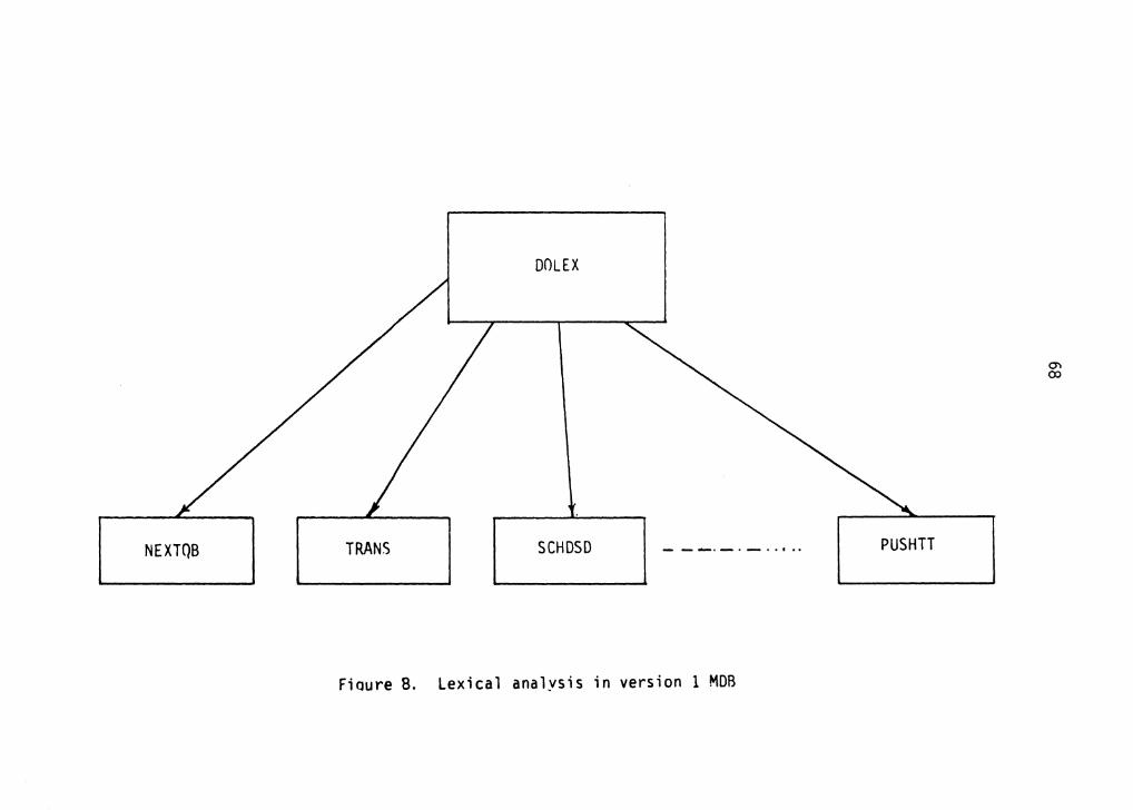
68
>< Li.J _
J
c Cl
I-I-::i::: V
l :::> c.. I 1 I
Cl
Vl
Cl
::i::: u V
l
~
z: ~
I-a:i
C"
I->< U
J z:
cc C
l ::E:
-c: 0 Ill ~
QJ > c: Ill
.,_. Ill >. ,.-IO
c: IO
,.-IO u
.,_. x QJ _
J
IX> cu s.. :l
0
'-'-

DOLEX
NEXTQB TRANS SCHDSD
ABORT AUTOSAVE SCH SELECT CHECK BEGIN
Fiqure 9. Lexical analysis in version 2 MOB
PUSH TT
EDIT LAST
0\ U)
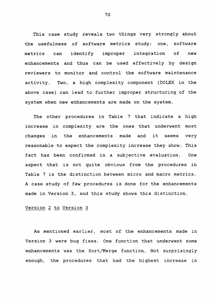
70
This case study reveals two things very strongly about
the usefulness of software metrics study: one, software
metrics can
enhancements
identify improper integration of new
and thus can be used effectively by design
reviewers to monitor and control the software maintenance
activity. Two, a high complexity component (DOLEX in the
above case) can lead to further improper structuring of the
system when new enhancements are made on the system.
The other procedures in Table 7 that indicate a high
increase in complexity are the ones that underwent most
changes in the enhancements made and it seems very
reasonable to expect the complexity increase they show. This
fact has been confirmed in a subjective evaluation. One
aspect that is not quite obvious from the procedures in
Table 7 is the distinction between micro and macro metrics.
A case study of few procedures is done for the enhancements
made in Version 3, and this study shows this distinction.
Version 2 to Version 3
As mentioned earlier, most of the enhancements made in
Version 3 were bug fixes. One function that underwent some
enhancements was the Sort/Merge function. Not surprisingly
enough, the procedures that had the highest increase in
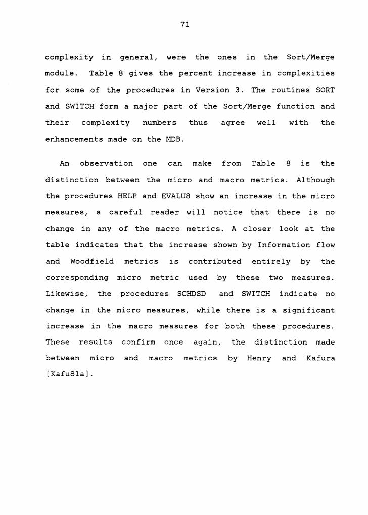
71
complexity in general, were the ones in the Sort/Merge
module. Table 8 gives the percent increase in complexities
for some of the procedures in Version 3. The routines SORT
and SWITCH form a major part of the Sort/Merge function and
their complexity numbers thus agree well with the
enhancements made on the MDB.
An observation one can make from Table 8 is the
distinction between the micro and macro metrics. Al though
the procedures HELP and EVALU8 show an increase in the micro
measures, a careful reader wi 11 notice that there is no
change in any of the macro metrics. A closer look at the
table indicates that the increase shown by Information flow
and Woodfield metrics is contributed entirely by the
corresponding micro metric used by these two measures.
Likewise, the procedures SCHDSD and SWITCH indicate no
change in the micro measures, while there is a significant
increase in the macro measures for both these procedures.
These results confirm once again, the distinction made
between micro and macro metrics by Henry and Kafura
[ Kafu81a] .
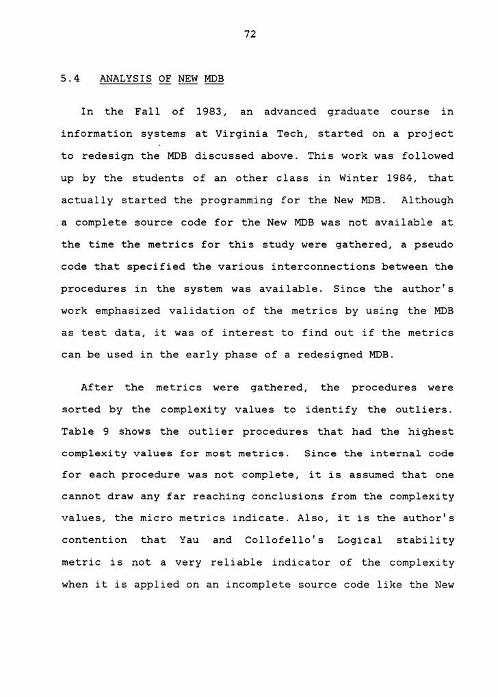
72
5.4 ANALYSIS OF NEW MDB
In the Fall of 1983, an advanced graduate course in
information systems at Virginia Tech, started on a project
to redesign the MDB discussed above. This work was followed
up by the students of an other class in Winter 1984, that
actually started the programming for the New MDB. Although
.a complete source code for the New MDB was not available at
the time the metrics for this study were gathered, a pseudo
code that specified the various interconnections between the
procedures in the system was available. Since the author's
work emphasized validation of the metrics by using the MDB
as test data, it was of interest to find out if the metrics
can be used in the early phase of a redesigned MDB.
After the metrics were gathered, the procedures were
sorted by the complexity values to identify the outliers.
Table 9 shows the outlier procedures that had the highest
complexity values for most metrics. Since the internal code
for each procedure was not complete, it is assumed that one
cannot draw any far reaching conclusions from the complexity
values, the micro metrics indicate. Also, it is the author's
contention that Yau and Collofello's Logical stability
metric is not a very reliable indicator of the complexity
when it is applied on an incomplete source code like the New
73
MDB. This is because, Yau and Collofello's metric considers
the ripple caused by the local variables and this ripple
effect cannot be identified in a procedure that does not
specify all the local variables that will eventually be used
when the system is complete. As it can be seen from the
table, the procedure VALUEMGT had a very high Information
flow complexity, as compared to any of the other procedures.
Since this was a rather abnormal procedure as indicated by
the metrics, these numbers were brought to the attention of
the project administrator for the New MDB.
Interestingly enough, the author was told by the project
administrator that he had an intuitive feeling, that the
procedure was not well structured and could become a
bottleneck in the future. It is obvious that the Information
flow complexity value for that procedure very strongly
indicates a possible poorly structured design. One useful
result of this evaluation was the decision by the project
managers to redesign the procedure, since it also performs a
major function of the New MDB. In the words of the project
director Dr. Rex Harston,
"The metrics generated for the New MDB spotted the modules which were causing the most confusion during the design process, allowing for appropriate adjustments during design. It is, therefore, my feeling that complexity measurement tools ought to be available as part of a system design support environment"
Chapter VI
CONCLUSIONS
This research has confirmed the results obtained in
previous work, with respect to the distinction between the
micro and macro metrics. These results indicate a strong
correlation between the micro metrics, as opposed to the
weak correlation of any of the micro metrics with the macro
metrics. A new inference drawn from the correlation
statistics amongst the macro metrics is that, they are all
distinct from each other and each of them measures a
different component of module interconnection complexity.
An analysis of three different versions of the same
system enabled us to study the power of software metrics in
monitoring,
activity.
and thus controlling,
The strength of this
the software maintenance
study
manual analysis of these enhancements,
lies in a careful
as indicated by the
design error in enhancements from Version 1 to Version 2 of
the Mini Data Base.
One major goal of software engineers is to apply the
software metrics at an early stage of a system design to
identify possible flaws in system structure and thus reduce
the associated software costs. Although to a limited extent,
74
75
this study has shown that it is possible to do that by
analyzing a redesign of the Mini Data Base system. An
interesting result of this analysis was the fact that, many
of the metrics cannot really be used at an early stage of
the system design, when the individual procedures of the
system are not completely written.
As mentioned earlier, most of the validation studies on
software metrics perform an analysis of correlation results
between the complexity metrics and the error history or the
programming time spent. This kind of study relies heavily on
the accuracy of the data collected for error history or
programming time, for the modules in the system. The error
count data collected on any large software system is usually
not very reliable, since in most cases, there are no uniform
set of rules to guide the programmer in counting errors.
Although it is possible to get accurate data about
programming time spent in a small controlled experiment,
this information is usually difficult to gather accurately
on any large software system. Also, the people in industry
are not likely to accept the idea of using software metrics
before some validation studies are done, that involve a
careful manual analysis of the results. This research makes
an effort in this direction and backs it up with a
subjective evaluation of the results by people familiar with
the system being analyzed.
76
One of the useful spinoffs from this research is the
availability of a software metric analyzer that computes a
set of software metrics. These metrics can be used in
analyzing the psychological complexity of a system more
usefully than relying on a small subset of the metrics. One
thing that the author realized while working with the data
generated is that it will be useful to develop an automated
tool for analyzing the different complexity numbers
generated. An example of such a system could be one that
uses a database for storing all the complexity values and
uses an information system that answers any statistical
queries about the metrics data.
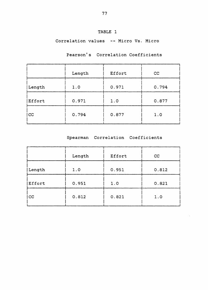
77
TABLE 1
Correlation values -- Micro Vs. Micro
Pearson's Correlation Coefficients
Length Effort cc
I I Length 1. 0 0.971 0.794
I I Effort 0.971 1. 0 0.877
I ICC 0.794 0.877 1. 0 I
Spearman Correlation Coefficients
Length Effort cc
I I Length 1. 0 0.951 0.812
I I Effort 0.951 1. 0 0.821
I ICC 0.812 0.821 1. 0 I
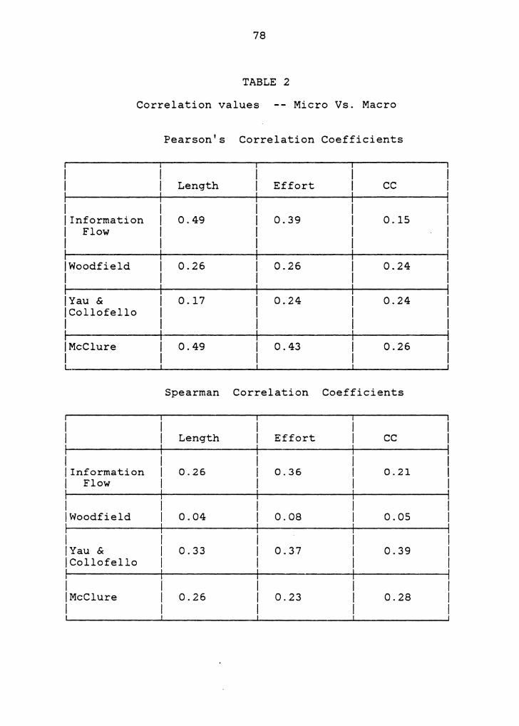
78
TABLE 2
Correlation values -- Micro Vs. Macro
Pearson's Correlation Coefficients
Length Effort cc
I I Information 0.49 0.39 0.15 I Flow I
I Woodfield 0.26 0.26 0.24 I !Yau & 0.17 0.24 0.24 ICollofello I
I McClure 0.49 0.43 0.26 I
Spearman Correlation Coefficients
Length Effort cc
I !Information 0.26 0.36 0.21 I Flow
I !Woodfield 0.04 0.08 0.05
I !Yau & 0.33 0.37 0.39 !Collofello
I I McClure 0.26 0.23 0.28 I
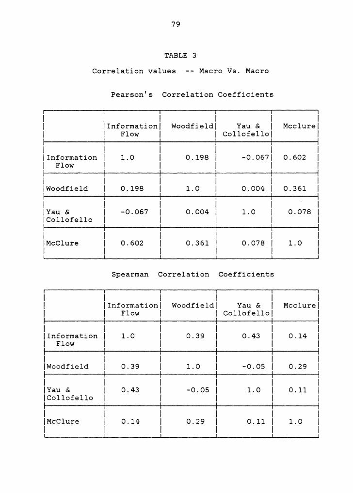
79
TABLE 3
Correlation values -- Macro Vs. Macro
Pearson's Correlation Coefficients
I I I I I I Information I Woodfield I Yau & I Mcclure I I Flow I I Collofellol I
I I I I Information 1.0 0.198 I -0.0671 0.602 I Flow I I
I I Woodfield 0.198 1. 0 0.004 0.361
I IYau & -0.067 0.004 1. 0 0.078 ICollofello
I I McClure 0.602 0.361 0.078 1. 0 I
Spearman Correlation Coefficients
I I I I I· IInformationl Woodfield I Yau & I Mcclure I I Flow I I Collofellol I
I I !Information 1.0 0.39 I 0.43 0.14 I Flow I
I !Woodfield 0.39 1. 0 -0.05 0.29
I IYau & 0.43 -0.05 1. 0 0.11 ICollofello
I I McClure 0 .14 0.29 0.11 1. 0 I
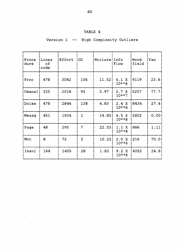
80
TABLE 4
Version 1 -- High Complexity Outliers
I I I I I I I I IProce I Lines I Effort ICC I Mcclure I Info I Wood I Yau ldure I of I I I I Flow I field I I I code I I I I I I
I I I I I I I IProc 478 I 3042 I 106 I 11. 52 I 4.1 x 19119 23.61 I I I I I 10**8 I I ICmanall 325 2018 93 5.97 2.7 x 15257 77.71 I I 10**7 I I IDolex 478 2844 I 138 4.83 2.4 x 18434 27.41 I I 10**8 I I IMessg 451 1934 I 1 14.851 4.5 x 15802 0.001 I I I 10**8 I I I Page 48 295 I 7 22.031 1.1 x 1886 1.11 I I I I 10**8 I I IMvc I e 72 I 3 10.221 2.0 x 1216 10.01 I I I I 10**6 I I I Inavi I 164 1405 28 1. 83 9.2 x 14052 24.81 I I 10**6 I I
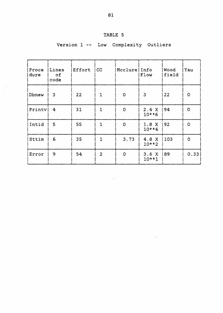
81
TABLE 5
Version 1 -- Low Complexity Outliers
I I I I I I I I IProce I Lines !Effort ICC I Mcclure I Info !Wood !Yau ldure I of I I I I Flow I field I I !code I I I I I I I I I I I I I IDbnew I 3 22 I 1 I 0 I 3 122 I o I I I I I I I IPrintvl 4 31 I 1 0 2.4 x 194 I o I I I 10**6 I I I Intid I 5 55 I 1 0 1.8 x 192 I o I I I 10**4 I I ISttim I 6 35 I 1 3.73 4.8 x 1103 I o I I I 10**2 I I !Error I 9 54 I 2 0 3.6 x 189 0.331 I I I 10**1 I I
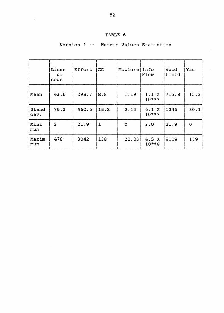
82
TABLE 6
Version 1 -- Metric Values Statistics
I I I I I I I !Lines !Effort ICC I Mcclure I Info !Wood !Yau I of I I I !Flow I field I !code I I I I I I
I I I I !Mean 43.6 298.7 18.8 1.19 1.1 x 1715.8 15.31 I I 10**7 I I !Stand 78.3 460.6 118.2 3.13 6.1 x 11346 20.11 ldev. I 10**7 I I !Mini I 3 21. 9 11 0 3.0 121. 9 I 0 !mum I I I I !Maxim 478 3042 1138 22.031 4. 5 x 19119 119 !mum I I 10**8 I
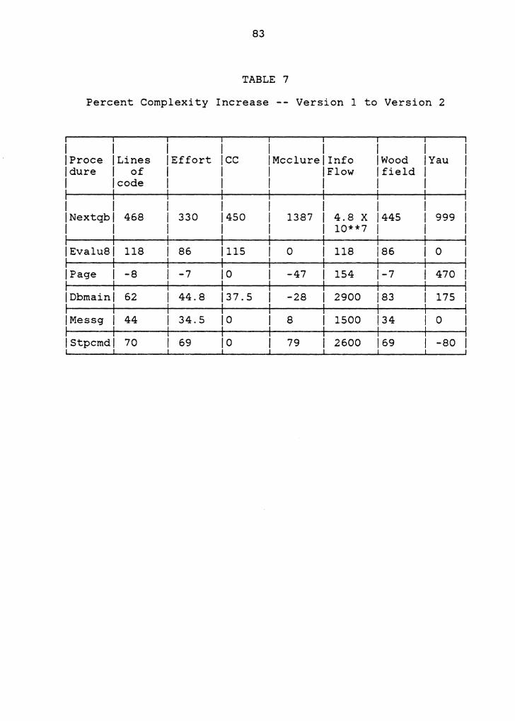
83
TABLE 7
Percent Complexity Increase -- Version 1 to Version 2
I I I I I I I I IProce !Lines !Effort ICC I Mcclure I Info !Wood !Yau ldure I of I I I !Flow I field I I !code I I I I I I I I I I INextqbl 468 330 1450 1387 4.8 x 1445 999 I I I 10**7 I
1Evalu81 118 86 1115 0 118 186 I o !Page -8 -7 10 -47 154 l-7 470
IDbmainl 62 44.8 137.5 -28 2900 183 175
IMessg I 44 34.5 10 8 1500 134 I o !Stpcmdl 70 69 10 79 2600 169 -80
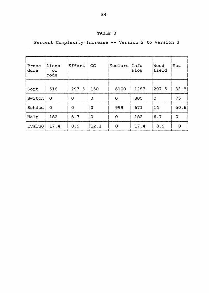
84
TABLE 8
Percent Complexity Increase -- Version 2 to Version 3
I I I I I I I I IProce I Lines !Effort ICC I Mee lure I Info !Wood !Yau ldure I of I I I !Flow I field I I !code I I I I I I
I I I I !Sort 516 297.5 1150 6100 1287 1297.5 33.81
!Switch! 0 I o 10 0 800 10 75
ISchdsdl 0 I o 10 999 671 114 I 50.61
!Help 182 6.7 10 0 182 16.7 I o 1Evalu81 17.4 8.9 112.1 0 17.4 I 8.9 0
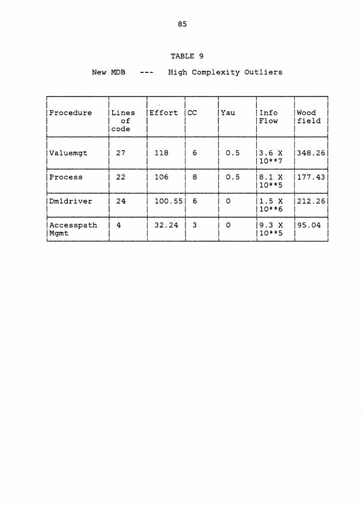
85
TABLE 9
New MDB High Complexity Outliers
I I I I I I I I !Procedure I Lines I Effort ICC I Yau I Info !Wood I I I of I I I !Flow I field I I !code I I I I I I I I I I I I IValuemgt 27 118 I 6 I 0.5 13.6 x I 348. 26 I I I I 110**7 I I !Process 22 106 I 8 0.5 j 8.1 x 1177.431 I I 110**5 I I IDmldriver I 24 100.551 6 I o j 1.5 X 1212.261 I I I I 110**6 I I IAccesspath I 4 32.24 I 3 I o 19.3 x 195.04 !Mgmt I I I 110**5 I

REFERENCES
[Anadoc] Comprehensive documentation " Software Metric Analyzer", by James Canning and Geereddy Reddy.
[Basi81] Basilli V., "Evaluating software development characteristics: Assessment of software measures in the software engineering laboratory", Proceedings of the sixth annual software engineering workshop, Dec 2, 1981.
[Boeh76] Boehm B.W, "Quantitative evaluation of software quality", Proceedings of 2nd International conference on software engineering. Oct. 1976.
[Boeh79] Boehm B.W, "Software engineering - As it is", Proceedings of 4th International conference on software engineering. Septl7-19 1979.
[Cook82] Cook M.L., "Software metrics An introduction and annotated bibliography", ACM SIGSOFT software engineering notes, Vol 7 no 2, April 1982.
[Curt79] Curtis W., Sheppard S., Milliman P., Borst M., Love T., "Measuring the psychological complexity of software maintenance tasks with the Halstead and McCabe Metrics", IEEE Transactions on software Engineering, Vol.SE-5,No.2, March 1979.
[Curt80] Curtis W., "Measurement and Experimentation in software engineering", Proceedings of the IEEE, Vol.68, No.9, Sept 1980.
[Fitz78] Fitzimmons A., Love T., "A review and evaluation of software science", ACM computing surveys, 10, 1 (March 1978), 3-18.
[Hame81] Hamer, Frewin, "Halstead's Software Science - A critical examination", ITT Technical Report No. STL 134, July 1981.
[Haye80] Hayes Mary, "An empirical study of measures of psychological complexity in software", Masters Thesis, University of California at Irvine, 1980.
[Henr79] Henry Sallie, "Information flow metrics for the evaluation of operating systems' structure", Ph.d Dissertation, Iowa state university, 1979.
86

87
[Kafu8la] Kafura D., Henry S., "Software quality metrics based on interconnectivity", The Journal of systems and software, Vol. 2, pp. 121-131, 1981.
[Kafu8lb] Kafura D., Henry S., "A viewpoint on software quality metrics: Criteria, Use and Interpretation", Proceedings of Sigsoft sponsored software engineering symposium, June 1981.
[Mcca76] McCabe T.J., "A complexity measure", IEEE transactions on software engineering, SE-2, December 1976, 308-320.
[McC178] McClure C., "A model for program complexity analysis", Proceedings 3rd international conference on software engineering, Atlanta, Ga. May 1978.
[MDBdoc] Documentation manual "The great new mini database", Project directed by Dr. Rex Hartson, VPI&SU, Dept. of computer science.
[Mill72] Mills H.D., "Mathematical foundations for structured programming", Federal systems division, IBM Corp., Gaithersburg, MD., FSC 72-6012, 1972.
[Myer75] Myers G.J., "Reliable software through composite design", Petrocelli/Charter, publisher 1975.
[Myer77] Myers G.J., "An extension to cyclomatic measure of program complexity", ACM Sigplan notices, Vol. 12, no. 10, Oct 1977, pp. 61-64.
[Otte81] Ottenstien L., "Predicting software development errors using software science parameters", Performance Evaluation Review : ACM workshop symposium on measurement and evaluation of software quality, March 1981.
[Ross77] Ross Douglas T., "Structured Analysis (SA}: A Language for communicating Ideas", IEEE transactions on software engineering, Jan 1977
[Schn79] Schneidewind N.F., Hoffman H.M., "An experiment in software error data collection and analysis", IEEE transactions on software engineering, Vol.SE-5, No.3. May 1979.
[Stro56] Stroud J.M., "The fine structure of psychological time", Information theory in psychology, The free press, Chicago Ill., 1956.
88
[Wood79] Woodfield S.N., "An experiment on unit increase in problem complexity", IEEE transactions on software engineering. SE-5, March 1979 76-79.
[Wood80] Woodfield S.N., "Enhanced effort estimation by extending basic programming models to include modularity factors", Ph.d. Thesis, Purdue university, computer science dept., 1980.
[Yau80] Yau S., Collofello J., "Some stability measures for software maintenance", IEEE transactions on software engineering, Vol. SE-6, No. 6, Nov 1980.

The vita has been removed from the scanned document