Application of repeated measurement ANOVA models using SAS and SPSS: examination of the effect of intravenous lactate infusion in Alzheimer's disease Krisztina

Application of repeated measurement Application of repeated measurement ANOVA models using SAS and SPSS:ANOVA models using SAS and SPSS:

examination of the effect of intravenous examination of the effect of intravenous lactate infusion in Alzheimer's diseaselactate infusion in Alzheimer's disease

Krisztina BodaKrisztina Boda11, János Kálmán, János Kálmán22, Zoltán Janka, Zoltán Janka22

Department of Medical InformaticsDepartment of Medical Informatics11, Department of Psychiatry, Department of Psychiatry22

University of Szeged, HungaryUniversity of Szeged, Hungary

MIE '2002 2

IntroductionIntroduction

Repeated measures analysis of variance (ANOVA) generalizes Student's t-test for paired samples. It is used when an outcome variable of interest is measured repeatedly over time or under different experimental conditions on the same subject.

MIE '2002 3

The purpose of the discussionThe purpose of the discussion

to show the application of different statistical models to investigate the effect of intravenous Na-lactate on cerebral blood flow and on venous blood parameters in Alzheimer's dementia (AD) probands using SAS and SPSS programs.

to show the most important properties of these statistical models.

to show that different models on the same data set may give different results.

MIE '2002 4

Topics of DiscussionTopics of Discussion The medical experiment

The data table

Statistical models and programs

Statistical analysis of two parameters (venous blood PH and systoloc blood pressure) using different models and programs GLM models Mixed models Comparison of the results

Summary of the key points

Medical results and discussion

MIE '2002 5

The medical experimentThe medical experiment

Patients: 20 patients having moderate-severe dementia syndrome (AD).

Experimental design: self-control study measurements were performed on the same patient

at 0, 10 and 20 minutes after 0.9 % NaCl (Saline) or 0.5 M Na-lactate infusion on two different days

NaCl (Saline) (day 1) Na-lactate (day 2)

0’ 10’ 20’ 0’ 10’ 20’

MIE '2002 6

The data The data „multivariate” or „wide” form„multivariate” or „wide” form

Proband PH1_0 PH1_10 PH1_20 PH2_0 PH2_10 PH2_20 PCO1_0 PCO1_101.00 7.43 7.42 7.43 7.42 . 7.46 34.60 34.502.00 7.39 7.39 7.39 7.36 7.36 7.43 50.40 48.703.00 7.37 7.38 7.38 7.40 7.45 7.46 45.60 46.904.00 7.43 7.42 7.42 7.43 7.45 7.48 48.20 47.105.00 7.39 7.39 7.39 7.38 7.40 7.42 44.50 44.606.00 7.36 7.39 7.41 7.32 7.39 7.45 47.20 48.007.00 7.38 7.39 7.38 7.37 7.41 7.46 48.10 49.508.00 7.39 7.40 7.39 7.36 7.44 7.48 44.40 46.609.00 7.34 7.39 7.41 7.34 7.41 7.45 50.10 49.8010.00 7.32 7.34 7.35 7.31 7.32 7.37 57.20 58.1011.00 7.40 7.38 7.39 7.34 7.40 7.47 42.70 45.0012.00 7.32 7.35 7.33 7.37 7.40 7.43 51.40 54.9013.00 . . . 7.42 7.43 7.48 . .14.00 7.42 7.41 7.39 7.42 7.42 7.43 43.20 49.2015.00 7.42 7.41 7.40 7.46 7.47 7.51 45.80 45.5016.00 7.37 7.36 7.36 7.37 7.36 7.41 53.60 55.1017.00 7.37 7.39 7.39 7.45 7.40 7.48 45.80 48.6018.00 7.39 7.38 7.37 7.42 7.40 7.44 42.50 43.1019.00 7.43 7.41 7.48 7.42 7.39 7.37 41.60 44.3020.00 . . . 7.41 7.46 7.45 . .20 18 18 18 20 19 20 18 18

MIE '2002 7

The data The data „univariate” or „long” form„univariate” or „long” form

MIE '2002 8

Statistical modelStatistical model

The statistical models will be shown using one chosen parameter the venous blood PH.

2 repeated measures factors: days (treatments) with 2 levels (Saline or Lactate) time with 3 levels (0, 10 and 20 minutes)

both factors are fixed values of interest are all represented in the data file

MIE '2002 9

Venous blood PH levelsVenous blood PH levels

2018 1918 2018N =

LactateSaline

PH

7.6

7.5

7.4

7.3

7.2

TIme

.00

10.00

20.00

69

111

59

•sample size

•interaction

MIE '2002 10


The data table


Statistical analysis of one parameter (venous blood PH) using different models and programs GLM models Mixed models Comparison of the results



MIE '2002 11

Statistical models and programsStatistical models and programs

t-tests the repeated use of the t-tests may increase the

experiment wise probability of Type I error.

ANOVA GLM Mixed

Programs used SAS 6.12, 8.02 SPSS 9.0, 11.0

MIE '2002 12

Repeated measures ANOVARepeated measures ANOVA

Observations on the same subject are usually correlated and often exhibit heterogeneous variability a covariance pattern across time periods can be

specified within the residual matrix.

Effects: between-subjects effects within-subjects effects

Interactions

MIE '2002 13

Statistical modelsStatistical models GLM (General Linear Model) y= X +

y: a vector of observed data : an unknown vector of fixed-effects parameters with known

design matrix X : an unknown random error vector – assumed to be

independently and identically distributed N(0,2) MIXED Model y= X + Z +

: an unknown vector of random-effects parameters with known design matrix Z

: an unknown random error vector – whose elements are no longer required to be independent and homogenous.

Assume that and are Gaussian random variables and have expectations 0 and variances G and R, respectively.

The variance of y is V=ZGZ’ + R For G and R some covariance structure must be selected

MIE '2002 14

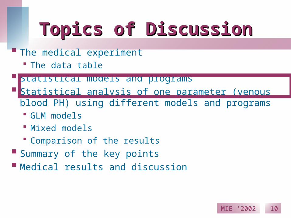
The within-subjects covariance matrix - The within-subjects covariance matrix - covariance patterns for 3 time periodscovariance patterns for 3 time periods

UN-Unstructured

CS-Compound Symmetry

232313

232212

131221

21

221

21

21

21

221

21

21

21

2

23

22

21

00

00

00

VC-Variance Components

AR(1) - First-Order Autoregressive

1

1

1

2

2

MIE '2002 15

GLMGLM MIXEDMIXED

Requires balanced data; subjects with missing observations are deleted

Assumes special form of the within-subject covariance matrix: Type H (Sphericity) – univariate

approach Unstructured –multivariate

approach

Estimates covariance parameters using a method of moments

….

Allows data that are missing at random

Allows a wide variety of within-subject covariance matrix UN-Unstructured VC-Variance Components CS-Compound Symmetry AR(1)-1th order autoregressive …

Estimates covariance parameters using restricted maximum likelihood,…

….

MIE '2002 16


The data table


Statistical analysis of one parameter (venous blood PH) using different models and programs GLM models Mixed models Comparison of the results



MIE '2002 17

Statistical analysis of venous blood PH Statistical analysis of venous blood PH using different models and programsusing different models and programs

Examination of univariate statistics and correlation structure

GLM univariate and multivariate results, verifying assumptions

Mixed models Create the model Examine and choose the covariance structure Compare fixed effects

MIE '2002 18

Paired Paired tt-test -test (only for demonstration –not recommended)(only for demonstration –not recommended)

Comparison Sig. (2-tailed)

Day 1, 0’-10’ 0.140

Day 1, 0’-20’ 0.164

Day 1, 10’-20’ 0.607

Day 2, 0’-10’ 0.009

Day 2, 0’-20’ 0.000

Day 2, 10’-20’ 0.000

0’, Day1-Day2 0.788

10’, Day1-Day2 0.018

20’, Day1-Day2 0.000

MIE '2002 19

Correlation of PH measurementsCorrelation of PH measurements PH1_0 PH1_10 PH1_20 PH2_0 PH2_10

PH2_20

PH1_0 1 .874 .691 .658 .512 .243

PH1_10 .874 1 .820 .600 .677 .407

PH1_20 .691 .820 1 .381 .296 .006

PH2_0 .658 .600 .381 1 .635 .399

PH2_10 .512 .677 .296. 635 1. 720

PH2_20 .243 .407 .006 .399 .720 1D1 T0

D1 T10

D1 T20

D2 T0

D2 T10

D2 T20

MIE '2002 20

Repeated measures ANOVARepeated measures ANOVA

Effects: between-subjects effects -none within-subjects effects

• Treatment (Saline - Lactate) - fixed

• Time (0’-10’-10’) - fixed

• Patient -random

Interactions Treatment*time interactions will be examined

MIE '2002 21

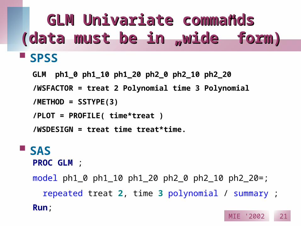
GLM Univariate commandsGLM Univariate commands(data must be in „wide” form)(data must be in „wide” form)

SPSS

SASPROC GLM ;

model ph1_0 ph1_10 ph1_20 ph2_0 ph2_10 ph2_20=;

repeated treat 2, time 3 polynomial / summary ;

Run;

GLM ph1_0 ph1_10 ph1_20 ph2_0 ph2_10 ph2_20

/WSFACTOR = treat 2 Polynomial time 3 Polynomial

/METHOD = SSTYPE(3)

/PLOT = PROFILE( time*treat )

/WSDESIGN = treat time treat*time.

MIE '2002 22

GLM univariate assumptions and results (SPSS)GLM univariate assumptions and results (SPSS)

Sphericity test failed, a correction can be applied

3 subjects are deleted because of missing value

TREATMENT*TIME interaction is significant

Tests of Within-Subjects Effects

Measure: MEASURE_1

1.569E-02 1 1.569E-02 11.277 .004

1.569E-02 1.000 1.569E-02 11.277 .004

1.569E-02 1.000 1.569E-02 11.277 .004

1.569E-02 1.000 1.569E-02 11.277 .004

2.226E-02 16 1.391E-03

2.226E-02 16.000 1.391E-03

2.226E-02 16.000 1.391E-03

2.226E-02 16.000 1.391E-03

2.109E-02 2 1.054E-02 20.718 .000

2.109E-02 1.350 1.562E-02 20.718 .000

2.109E-02 1.430 1.475E-02 20.718 .000

2.109E-02 1.000 2.109E-02 20.718 .000

1.629E-02 32 5.089E-04

1.629E-02 21.596 7.541E-04

1.629E-02 22.875 7.119E-04

1.629E-02 16.000 1.018E-03

1.227E-02 2 6.133E-03 14.171 .000

1.227E-02 1.501 8.174E-03 14.171 .000

1.227E-02 1.622 7.564E-03 14.171 .000

1.227E-02 1.000 1.227E-02 14.171 .002

1.385E-02 32 4.328E-04

1.385E-02 24.012 5.768E-04

1.385E-02 25.947 5.338E-04

1.385E-02 16.000 8.656E-04

Sphericity Assumed

Greenhouse-Geisser

Huynh-Feldt

Lower-bound

Sphericity Assumed

Greenhouse-Geisser

Huynh-Feldt

Lower-bound

Sphericity Assumed

Greenhouse-Geisser

Huynh-Feldt

Lower-bound

Sphericity Assumed

Greenhouse-Geisser

Huynh-Feldt

Lower-bound

Sphericity Assumed

Greenhouse-Geisser

Huynh-Feldt

Lower-bound

Sphericity Assumed

Greenhouse-Geisser

Huynh-Feldt

Lower-bound

SourceTREAT

Error(TREAT)

TIME

Error(TIME)

TREAT * TIME

Error(TREAT*TIME)

Type III Sumof Squares df Mean Square F Sig.

1.629E-02 16.000 1.018E-03

1.227E-02 2 6.133E-03 14.171 .000

1.227E-02 1.501 8.174E-03 14.171 .000

1.227E-02 1.622 7.564E-03 14.171 .000

1.227E-02 1.000 1.227E-02 14.171 .002

Lower-bound

Sphericity Assumed

Greenhouse-Geisser

Huynh-Feldt

Lower-bound

Error(TIME)

TREAT * TIME

MIE '2002 23

GLM multivariate results (SPSS)GLM multivariate results (SPSS)

Multivariate Testsb

.413 11.277a 1.000 16.000 .004

.587 11.277a 1.000 16.000 .004

.705 11.277a 1.000 16.000 .004

.705 11.277a 1.000 16.000 .004

.724 19.651a 2.000 15.000 .000

.276 19.651a 2.000 15.000 .000

2.620 19.651a 2.000 15.000 .000

2.620 19.651a 2.000 15.000 .000

.537 8.702a 2.000 15.000 .003

.463 8.702a 2.000 15.000 .003

1.160 8.702a 2.000 15.000 .003

1.160 8.702a 2.000 15.000 .003

Pillai's Trace

Wilks' Lambda

Hotelling's Trace

Roy's Largest Root

Pillai's Trace

Wilks' Lambda

Hotelling's Trace

Roy's Largest Root

Pillai's Trace

Wilks' Lambda

Hotelling's Trace

Roy's Largest Root

EffectTREAT

TIME

TREAT * TIME

Value F Hypothesis df Error df Sig.

Exact statistica.

Design: Intercept Within Subjects Design: TREAT+TIME+TREAT*TIME

b.

MIE '2002 24

Plot in SPSSPlot in SPSS

Estimated Marginal Means of MEASURE_1

TIME

321

Est

ima

ted

Ma

rgin

al M

ea

ns

7.45

7.44

7.43

7.42

7.41

7.40

7.39

7.38

7.37

TREAT

1

2

Estimated Marginal Means of MEASURE_1

TIME

321

Est

ima

ted

Ma

rgin

al M

ea

ns

7.45

7.44

7.43

7.42

7.41

7.40

7.39

7.38

7.37

TREAT

1

2

MIE '2002 25

Mixed models commandsMixed models commands(Data must be in „long” form)(Data must be in „long” form)

SAS 8.02

SPSS 11.0

proc mixed covtest;

class name treat time;

model ph = treat time treat*time;

repeated /type=un sub=name r rcorr;

lsmeans treat*time /pdiff;

run;

MIXED ph BY treat time /CRITERIA = CIN(95) MXITER(100) MXSTEP(10) SCORING(1) SINGULAR(0.000000000001) HCONVERGE(0, ABSOLUTE) LCONVERGE(0, ABSOLUTE) PCONVERGE(0.000001, ABSOLUTE) /FIXED = treat time time*treat | SSTYPE(3) /METHOD = REML /PRINT = G LMATRIX R SOLUTION TESTCOV /REPEATED = treat time | SUBJECT(name ) COVTYPE(UN) /SAVE = RESID .

MIE '2002 26

Selecting the covariance structureSelecting the covariance structure

Using SAS command, replacing “UN” in type=UN with CS, VC, HF , AR(1) and others defines Unstructured, Variance Components, Huynh-Feldt and First Order Autoregressive, etc… variance-covariance structures of the fixed effects. The default is VC.

Using SPSS command, replacing “UN” in COVTYPE(UN) with ID, CS, VC, HF , AR(1) defines the above covariance structures. No other types are available.

MIE '2002 27


The unstructured covariance is overly complex. In our example we have 6 levels for treat*time effects, so the unstructured covariance has 6 variances and 15 covariances (6*5)/2 ), for a total of 21 variances and covariances being estimated. The other structures use less covariance parameter for the repeated effects.

Another problem with CS, HF and AR(1) structures that they do not take into account the double repeated nature of our model.

MIE '2002 28


Correlation matrix for a block using UN covariance structure

Row COL1 COL2 COL3 COL4 COL5 COL6

1 1.00000000 0.87572288 0.69284518 0.64717994 0.54989785 0.24762745

2 0.87572288 1.00000000 0.82563330 0.59373944 0.69760124 0.39606241

3 0.69284518 0.82563330 1.00000000 0.37105322 0.36385899 0.00696442

4 0.64717994 0.59373944 0.37105322 1.00000000 0.64283355 0.39879596

5 0.54989785 0.69760124 0.36385899 0.64283355 1.00000000 0.71658187

6 0.24762745 0.39606241 0.00696442 0.39879596 0.71658187 1.00000000

Correlation matrix for a block using AR(1) covariance structure

Row Col1 Col2 Col3 Col4 Col5 Col6

1 1.0000 0.6169 0.3805 0.2348 0.1448 0.08933

2 0.6169 1.0000 0.6169 0.3805 0.2348 0.1448

3 0.3805 0.6169 1.0000 0.6169 0.3805 0.2348

4 0.2348 0.3805 0.6169 1.0000 0.6169 0.3805

5 0.1448 0.2348 0.3805 0.6169 1.0000 0.6169

6 0.08933 0.1448 0.2348 0.3805 0.6169 1.0000

MIE '2002 29

Selecting the covariance structure: Selecting the covariance structure:

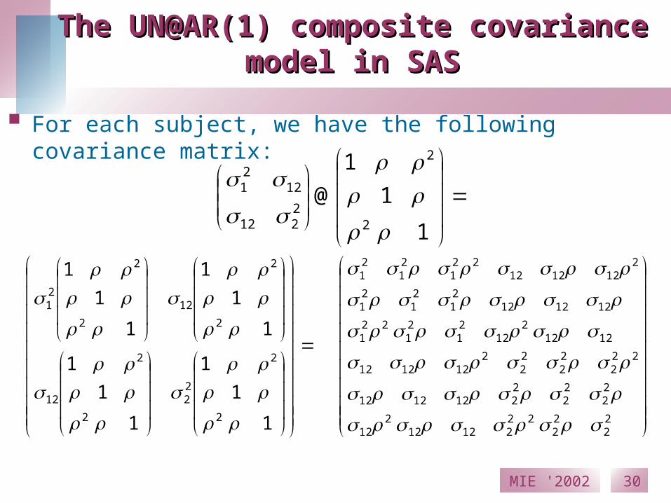
aa composite covariance model composite covariance model Under a composite covariance model separate

covariance structures are specified for each of two repeat factors. Using UN@AR(1), we assume equal correlation between treatments (UN) and AR(1) covariance structure between the three time points.

UN@AR(1): we assume the UN covariance matrix for the treatments and the AR(1) covariance matrix for the time effects

MIE '2002 30

The UN@AR(1) composite covariance The UN@AR(1) composite covariance model in SASmodel in SAS

For each subject, we have the following covariance matrix:

1

1

1

1

1

1

1

1

1

1

1

1

2

2

22

2

2

12

2

2

12

2

2

21

22

22

2221212

212

22

22

22121212

222

22

22

2121212

12122

1221

21

221

12121221

21

21

2121212

221

21

21

1

1

1

@2

2

2212

1221

MIE '2002 31


Correlation matrix for a block using UN@AR(1) covariance structure

Row COL1 COL2 COL3 COL4 COL5 COL6

1 1.00000000 0.73001496 0.53292185 0.22698641 0.16570348 0.12096602 2 0.73001496 1.00000000 0.73001496 0.16570348 0.22698641 0.16570348 3 0.53292185 0.73001496 1.00000000 0.12096602 0.16570348 0.22698641 4 0.22698641 0.16570348 0.12096602 1.00000000 0.73001496 0.53292185 5 0.16570348 0.22698641 0.16570348 0.73001496 1.00000000 0.73001496 6 0.12096602 0.16570348 0.22698641 0.53292185 0.73001496 1.00000000

Correlation between time Time 0 Time 10 Time 20 Time 0 1.00000000 0.73001496 0.53292185 Time 10 0.73001496 1.00000000 0.73001496 Time 20 0.53292185 0.73001496 1.00000000

R=0.227 (correlation between treatments)

MIE '2002 32

Comparison of mixed models with Comparison of mixed models with different covariance structuresdifferent covariance structures

Based on information criteria about the model fit Akaike's Information Criterion (AIC) -2 Restricted Log Likelihood:

• Likelihood ratio test (for nested models)

Smaller values indicate better models

MIE '2002 33

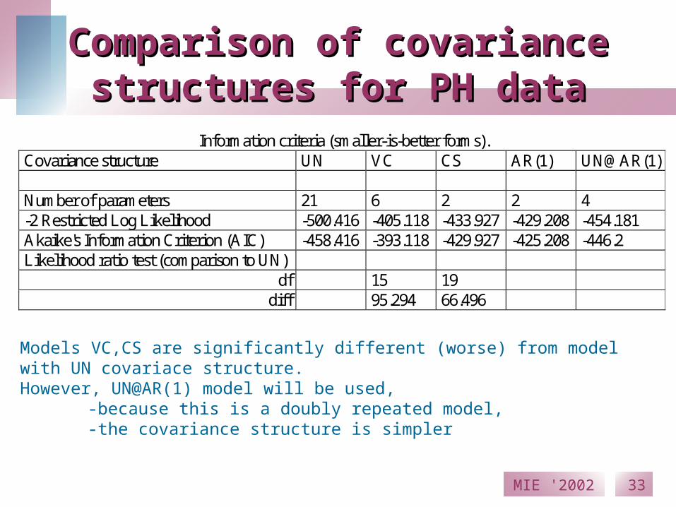
Comparison of covariance Comparison of covariance structures for PH datastructures for PH data

Information criteria (smaller-is-better forms). Covariance structure UN VC CS AR(1) UN@AR(1) Number of parameters 21 6 2 2 4 -2 Restricted Log Likelihood -500.416 -405.118 -433.927 -429.208 -454.181 Akaike's Information Criterion (AIC) -458.416 -393.118 -429.927 -425.208 -446.2 Likelihood ratio test (comparison to UN)

df 15 19 diff 95.294 66.496

Models VC,CS are significantly different (worse) from model with UN covariace structure. However, UN@AR(1) model will be used,

-because this is a doubly repeated model,-the covariance structure is simpler

MIE '2002 34

Results using mixed model (SAS)Results using mixed model (SAS)

Tests of Fixed Effects (Type=UN@AR)

Source NDF DDF Type III F Pr > F

TREAT 1 88 8.77 0.0039

TIME 2 88 15.86 0.0001

TREAT*TIME 2 88 14.22 0.0001

MIE '2002 35

Differences of Least Squares MeansDifferences of Least Squares Means

Differences of Least Squares Means

Effect TREAT TIME _TREAT _TIME Difference Std Error DF t Pr > |t|

TREAT*TIME 1.00 0.00 1.00 10.00 -0.00668 0.004978 33 -1.34 0.1886 TREAT*TIME 1.00 0.00 1.00 20.00 -0.00888 0.006548 33 -1.36 0.1844 TREAT*TIME 1.00 10.00 1.00 20.00 -0.00219 0.004978 33 -0.44 0.6624 TREAT*TIME 2.00 0.00 2.00 10.00 -0.02260 0.006852 33 -3.30 0.0023 TREAT*TIME 2.00 0.00 2.00 20.00 -0.05895 0.008888 33 -6.63 <.0001 TREAT*TIME 2.00 10.00 2.00 20.00 -0.03635 0.006852 33 -5.30 <.0001

TREAT*TIME 1.00 0.00 2.00 0.00 -0.00459 0.01018 33 -0.45 0.6551 TREAT*TIME 1.00 10.00 2.00 10.00 -0.02051 0.01024 33 -2.00 0.0536 TREAT*TIME 1.00 20.00 2.00 20.00 -0.05466 0.01018 33 -5.37 <.0001

Paired t-test: Comparison Sig. (2-tailed) Day 1, 0’-10’ 0.140

Day 1, 0’-20’ 0.164 Day 1, 10’-20’ 0.607 Day 2, 0’-10’ 0.009 Day 2, 0’-20’ 0.000 Day 2, 10’-20’ 0.000 0’, Day1-Day2 0.788 10’, Day1-Day2 0.018 20’, Day1-Day2 0.0002018 1918 2018N =

LactateSaline

PH

7.6

7.5

7.4

7.3

7.2

TIme

.00

10.00

20.00

69

111

59

MIE '2002 36

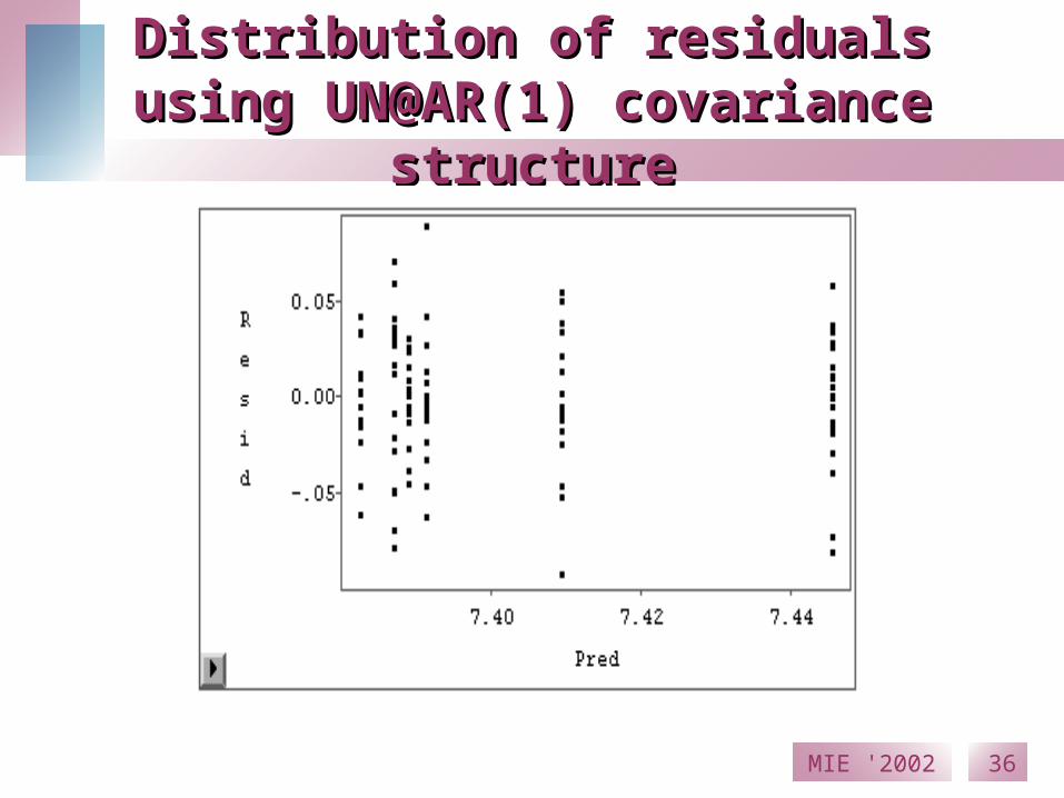
Distribution of residuals using Distribution of residuals using UN@AR(1) covariance structureUN@AR(1) covariance structure

MIE '2002 37

Summary of statistical results Summary of statistical results for venous blood PH for venous blood PH

Changing models might give different results. GLM models are useful in case of balanced data

satisfying special assumptions. Using mixed model, the covariance structure of

repeated effects can be taken into account, and cases with missing values are not deleted.

The presence of a treatment*time interaction is obvious by any model.

MIE '2002 38

Examination of another parameter: Examination of another parameter: systolic blood pressure (RRS)systolic blood pressure (RRS)

1919 1819 1919N =

LactateSaline

RR

s

200

180

160

140

120

100

80

Time

0

10

20 RRS 2-20RRS 2-10RRS 2-0RRS 1-20RRS 1-10RRS 1-0

200

180

160

140

120

100

80

MIE '2002 39

Mean and SD of systolic blood pressure

0.00

20.00

40.00

60.00

80.00

100.00

120.00

140.00

160.00

180.00

0 10 20

Time (min)

Hg

mm Saline

Lactate

N 19 19 19 19

MIE '2002 40

Mean of systolic blood pressure

138.89

140.26

146.89

142.05

139.74140.61

130.00

132.00

134.00

136.00

138.00

140.00

142.00

144.00

146.00

148.00

150.00

0 10 20 Time (min)

Hg

mm Saline

Lactate

N 19 19 19 19 18 19

Mean of systolic blood pressure

138.17 138.67

144.83

141.11

138.50

140.61

130.00

132.00

134.00

136.00

138.00

140.00

142.00

144.00

146.00

148.00

150.00

0 10 20 Time (min)

Hg

mm Saline

Lactate

N 18 18 18 18 18 18

Different sample size Equal sample size

The same figure with different scalingThe same figure with different scaling

MIE '2002 41

GLM results (2 cases are deleted)GLM results (2 cases are deleted)

GLM Multivariate (Wilks’ Lambda Sig): TREAT 0.868 TIME 0.095 TREAT*TIME 0.270

GLM Univariate (Spericity assumptions met) TREAT 0.868 TIME 0.042 TREAT*TIME 0.253

Is there a significant time effect?

0.042

0.095

MIE '2002 42

Plot in SPSS GLMPlot in SPSS GLM

Estimated Marginal Means

TIME

20100

Est

ima

ted

Ma

rgin

al M

ea

ns

148

146

144

142

140

138

TREATMENT

Saline

Lactate

MIE '2002 43

Correlation matrix of systolic blood pressuresCorrelation matrix of systolic blood pressures

BP1_0 BP1_10 BP1_20 BP2_0 BP2_10 BP2_20

BP1_0 1 .954 .893 .884 .619 .790

BP1_10 .954 1 .908 .842 .569 .776

BP1_20 .893 .908 1 .825 .566 .778

BP2_0 .884 .842 .825 1 .755 .791

BP2_10 .619 .569 .566 .755 1 .825

BP2_20 .790 .776 .778 .791 .825 1

Paired t-tests Sig. (2-tailed)RRS 1-0 - RRS 1-10 .409

RRS 1-0 - RRS 1-20 .003

RRS 1-10 - RRS 1-20 .009

RRS 2-0 - RRS 2-10 .515

RRS 2-0 - RRS 2-20 .439

RRS 2-10 - RRS 2-20 .845

RRS 1-0 - RRS 2-0 .715

RRS 1-10 - RRS 2-10 .672

RRS 1-20 - RRS 2-20 .155

MIE '2002 44

MIXED: Comparison MIXED: Comparison of covariance structures for BP dataof covariance structures for BP data

Information criteria (smaller-is-better forms).UN VC CS HF AR(1) UN@AR(1)

Covariance structureNumber of parameters 21 6 2 7 2 4-2 Restricted Log Likelihood 815.637 968.25 858.587 853.88 848.541 860.93Akaike's Information Criterion (AIC) 857.637 978.1 862.587 868.337 852.546 868.9Likelihood ratio test (comparison toUN)

df 15 19 14 19 17diff 152.613 42.95 38.243 32.9 46.29

p <0.0001 .001317 .000477 .024686 .000156

UN covariance structure is significantly better than the other models examined

MIE '2002 45

Results for time-trend Results for time-trend using mixed modelusing mixed model

GLM: based on data of 18 patients, univariate results seem to be acceptable, showing a significant time-trend. However, assumptions of the multivariate approach are more realistic. Multivariate (UN): 2, 16, p=0.095 Univariate (CS): 2, 34 p=0.042.

MIXED: based on data of 20 patients, UN covariance structure has to be used. UN: 2, 18, p=0.045 CS: 2, 89 p=0.0587

The p-values are close. There is a significant increase in time for BP data.

MIE '2002 46

Using mixed models, an increasing time effect could be shown.

MIE '2002 47

Covariance pattern model vs. Covariance pattern model vs. random coefficients modelrandom coefficients model

When correlation between observations on the same patients is not constant, a covariance pattern model can be used.

When the relationship of the response variable with time is of interest, a random coefficients model is more appropriate. Here, regression curves are fitted for each patient and the regression coefficients are allowed to vary randomly between the patients.

MIE '2002 48

Individual regression linesIndividual regression lines

TREAT: 1.00 Saline

Time

3020100-10

RR

s

200

180

160

140

120

100

TREAT: 2.00 Lactate

Time

3020100-10R

Rs

200

180

160

140

120

100

80

MIE '2002 49

SAS commandsSAS commands1. Fixed effects approach (linear regression with one independent

variable). The effect of patient is ignored – all observations are treated as independent.

proc mixed;model rrs= time /s;run;

2. Mixed models (with random coefficients for patients and patients*time)proc mixed;class name treat;model rrs= time /s;random int time /sub=name type=un solution;run;

3. Mixed models with two additional effects (with random coefficients for patients and patients*time)

proc mixed;class name treat;model rrs=treat time treat*time/s;random int time /sub=name type=un solution;run;

MIE '2002 50

Regression lines by averaged by treatmentsRegression lines by averaged by treatments

Time

3020100-10

RR

s200

180

160

140

120

100

Treatment

Lactate

Saline

MIE '2002 51

Results I: fixed effects (linear regression)Results I: fixed effects (linear regression)

Covariance Parameter Estimates: Residual 410.02

Fit Statistics

-2 Res Log Likelihood 996.5

Solution for Fixed Effects Effect Estimate Standard Error DF t Value Pr > |t|

Intercept 138.84 3.0039 111 46.22 <.0001TIME 0.2579 0.2323 111 1.11 0.2693

Type 3 Tests of Fixed Effects

Num DenEffect DF DF F Value Pr > F

TIME 1 111 1.23 0.2693 The time-effect is not significant

Residual variance: 410.02

RRS=0.2579*time + 138.84

MIE '2002 52

Results I: fixed effects (linear regression)Results I: fixed effects (linear regression)

Time

3020100-10

RR

s

200

180

160

140

120

100

80

Treatment

Lactate

Saline

Total Population

RRS=0.2579*time + 138.84

The time-effect is not significant

MIE '2002 53

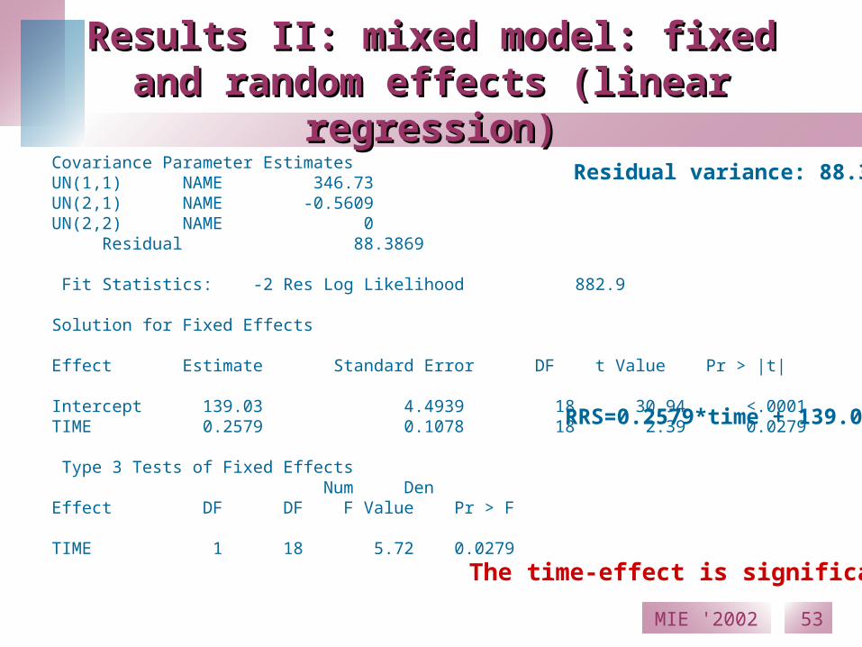
Results II: mixed model: fixed and Results II: mixed model: fixed and random effects (linear regression)random effects (linear regression)

Covariance Parameter EstimatesUN(1,1) NAME 346.73UN(2,1) NAME -0.5609UN(2,2) NAME 0 Residual 88.3869

Fit Statistics: -2 Res Log Likelihood 882.9

Solution for Fixed Effects

Effect Estimate Standard Error DF t Value Pr > |t|

Intercept 139.03 4.4939 18 30.94 <.0001TIME 0.2579 0.1078 18 2.39 0.0279

Type 3 Tests of Fixed Effects Num DenEffect DF DF F Value Pr > F

TIME 1 18 5.72 0.0279


RRS=0.2579*time + 139.03

The time-effect is significant

MIE '2002 54

Results III: mixed model: two fixed Results III: mixed model: two fixed effects and random effectseffects and random effects

Covariance Parameter EstimatesUN(1,1) NAME 346.73UN(2,1) NAME -0.5609UN(2,2) NAME 0 Residual 88.3869 Fit Statistics

-2 Res Log Likelihood 879.2

Type 3 Tests of Fixed Effects Num DenEffect DF DF F Value Pr > F

TREAT 1 73 0.53 0.4703TIME 1 18 5.71 0.0280TIME*TREAT 1 73 1.74 0.1919


The time-effect is significant

The other two effects are not significant

We decide to use MODEL II

MIE '2002 55

DiscussionDiscussion

Using statistical software without knowing their main properties or using only their default parameters may lead to spurious results.

Using only the default parameters means that simple models are supposed (i.e. VC covariance pattern in mixed procedure).

Medical experiments often result in repeated measures data, nested repeated measures data. The use of carefully chosen statistical model may improve the quality of statistical evaluation of medical data.

MIE '2002 56

Medical consequencesMedical consequences

The main results are that the diminished elevation of serum cortisol levels indicates blunted stress response to Na-lactate in AD. The decreased vascular responsiveness of the majority of AD cases reflects impaired vasoreactivity and disturbed vasoregulation. Since the catecholaminerg system and cholinergic mechanisms are also involved in the regulation of reactivity of the brain microvasculature, these alterations might be the consequences of the general cholinergic deficit in AD.

MIE '2002 57

ReferencesReferences

1. H. Brown and R. Prescott, Applied Mixed Models in Medicine. Wiley, 2001.

2. SAS Institute, Inc: The MIXED procedure in SAS/STAT Software: Changes and Enhancements through Release 6.11. Copyright © 1996 by SAS Institute Inc., Cary, NC 27513.

3. T. Park, and Y.J. Lee,: Covariance models for nested repeated measures data: analysis of ovarian steroid secretion data. Statistics in Medicine 21 (2002) 134-164

4. SPSS Advanced Models 9.0. Copyright © 1996 by SPSS Inc P. 5. R. S. Stewart, M. D. Devous, A. J. Rush, L. Lane, F. J. Bonte, Cerebral

blood flow changes during sodium-lactate induced panic attacks. Am. J. Psych., 145 (1988) 442-449.

6. R. Wolfinger and M. Chang, Comparing the SAS GLM and MIXED Procedures for Repeated Measures, SAS Institute Inc., Cary, NC. http://www.ats.ucla.edu/stat/sas/library/

Documents

Application of repeated measurement ANOVA models using SAS and SPSS: examination of the effect of intravenous lactate infusion in Alzheimer's disease Krisztina