APPLICATION OF PUSH-RELABEL AND HEURISTICS TO OPEN PIT

APPLICATION OF PUSH-RELABEL AND HEURISTICS TO OPEN PIT MINES

by

JASPREET SAHNI

M.B.A., Simon Fraser University, 1992

M.Sc., The University of British Columbia, 1996

A THESIS SUBMITTED IN PARTIAL FULFILLMENT OF

T H E REQUIREMENTS FOR T H E D E G R E E OF

M A S T E R OF SCIENCE

in

T H E F A C U L T Y OF G R A D U A T E STUDIES

(Department of Commerce)

We accept this thesis as conforming

to the required standard

T H E UNIVERSITY OF BRITISH COLUMBIA

October 1996

( C ) J a s p r e e t S a h n i , 1996

In presenting this thesis in partial fulfilment of the requirements for an advanced

degree at the University of British Columbia, I agree that the Library shall make it

freely available for reference and study. I further agree that permission for extensive

copying of this thesis for scholarly purposes may be granted by the head of my

department or by his or her representatives. It is understood that copying or

publication of this thesis for financial gain shall not be allowed without my written

permission.

Department of C o ^ i ^ e r t a and- © u s i ^ e s c , A . d m i r t t s ' T r a \ 100

The University of British Columbia Vancouver, Canada

Date D e c ^ w x b - e v H , ' °> S fe

-6 (2/88)

A b s t r a c t

The p i t l i m i t problem i s c r u c i a l to mine plan n i n g . The us of computer models to design u l t i m a t e open p i t l i m i t s i s becoming i n c r e a s i n g l y popular. One s o l u t i o n method adopted i s to transform the p i t l i m i t problem to a maximum flow network. A popular maximum flow technique i s push r e l a b e l . The purpose of t h i s t h e s i s i s twofold. The f i r s t i s to check i f push r e l a b e l a l g o r i t h m performs b e t t e r than other MF algorithms on r e a l , r a t h e r than randomly generated data (as i n the p a s t ) . The second i s to develop and t e s t h e u r i s t i c s that can take advantage of the c h a r a c t e r i s t i c s of the open p i t mine network s t r u c t u r e to f u r t h e r enhance the push r e l a b e l r o u t i n e .

ii

T a b l e o f C o n t e n t s

A b s t r a c t i i Table of Contents i i

L i s t of Tables i v L i s t of Figures V

Acknowledgement v i

Chapter One I n t r o d u c t i o n 1

Chapter Two M o d e l l i n g 4

Chapter Three Op t i m i s a t i o n Techniques 6

Graph Theory- 8

Two dimensional dynamic programming 9

Three dimensional dynamic programming 10

Lin e a r programming 12

Network Flow 13

FKS c l o s u r e a l g o r i t h m 15

Johnson's Network flow 17

Push Relabel 19

H e u r i s t i c s 22

Chapter Four Our Implementation 24

Various H e u r i s t i c s 28

I l l u s t r a t i v e example 39

Chapter Five Results and Conclusions 47

Tables and Figures 55

References 70

iii

L I S T O F T A B L E S

S o l u t i o n Times T o t a l Times FKS D i n i c

Push R e l a b e l (FIFO) H e u r i s t i c

Push R e l a b e l (HL) H e u r i s t i c

Expanded

iv

L I S T O F F I G U R E S

S o l u t i o n time S o l u t i o n time (no FKS) S o l u t i o n time S o l u t i o n time (no FKS) T o t a l time

Log S o l u t i o n time vs. Log Nodes

A c k n o w l e d g e m e n t

I would l i k e to thank a l l the members of my committee f o r t h e i r time and patience. In p a r t i c u l a r my s u p e r v i s o r Dr Tom McCormick deserves s p e c i a l r e c o g n i t i o n f o r h i s time spent i n numerous meetings o r g a n i s i n g my research. I would l i k e to acknowledge the help of Lynx Geosystems, Inc. f o r p r o v i d i n g mine data (blockmod and s a b o 2 ) and the code f o r generating the .spp and .spv f i l e s . I would a l s o l i k e to thank Todd Stewart f o r w r i t i n g the network generator code.

F i n a l l y , I thank my e n t i r e f a m i l y , e s p e c i a l l y my parents and wife Meera, f o r t h e i r constant support and encouragement.

vi

C H A P T E R 1

I n t r o d u c t i o n

Mine planning c o n s i s t s of determining a sequence of

e x t r a c t i o n over a given time horizon. The optimum open-pit

l i m i t of a mine i s defined by Caccetta and Giannini (1990) to

be a f e a s i b l e contour whose e x t r a c t i o n r e s u l t s i n maximum

t o t a l p r o f i t . F e a s i b i l i t y necessitates the p i t to have safe

and workable w a l l slopes which depend on the g e o l o g i c a l

structure and the mining equipment. The ultimate p i t l i m i t s

a f f e c t the e n t i r e mine layout and provide e s s e n t i a l

information f o r the evaluation of the economic p o t e n t i a l of

the mineral deposit and i n formulating long, intermediate,

and short range mine plans. Consequently, knowledge of the

optimum p r o f i t a b l e ultimate p i t l i m i t s during the i n i t i a l

stages can avoid c e r t a i n problems such as mining u n p r o f i t a b l e

expansions, abandoning p r o f i t a b l e ore, and r e l o c a t i n g surface

f a c i l i t i e s .

A mine planning s i t u a t i o n requires d i f f e r e n t l e v e l s of

p r e c i s i o n at each stage. Johnson (1973) argues that a good

estimation of the p i t l i m i t provides a s a t i s f a c t o r y b a s i s f o r

the i n i t i a l f e a s i b i l i t y evaluation of a mining p r o j e c t . But

knowledge of the true optimum becomes more valuable as mine

l i f e progresses and the knowledge of each aspect of the

operation increases. The a v a i l a b i l i t y of accurate economic

1

p i t l i m i t s f o r intermediate range planning leads to b e t t e r

scheduling r e s u l t i n g i n increased p r o f i t a b i l i t y f o r the

project. The ultimate decision to abandon an open-pit mining

venture requires that the p i t l i m i t c a l c u l a t i o n be nothing

short of optimum. Unfortunately, i n the past the techniques

that guarantee optimum so l u t i o n s have been too complex to be

understood by the mining community or too c o s t l y to implement

i n terms of computer processing times. This r e s u l t s i n the

use of simple and f a s t h e u r i s t i c s . A l l stages of mine

planning may therefore b e n e f i t from a technique which

provides an optimal s o l u t i o n at a low cost and i n an e a s i l y

understood manner.

One technique used to provide the optimal p i t l i m i t i s

to transform the network i n t o a maximum flow problem. The

maximum flow problem can then be solved with many standard

r o u t i n e s of which the one with the best reputation f o r

p r a c t i c a l performance i s push-relabel. This t h e s i s shows

that network implementations which i n the past have been

regarded to be too slow, are indeed very f a s t now. I t

assesses the push r e l a b e l algorithm's performance as compared

to other maximum-flow algorithms on ac t u a l c l a s s of graphs

(open p i t mining) rather than randomly generated data as has

been done i n the past at the DIMACS Challenge (Cherkassky and

Goldberg 1994). Also, we attempt to take advantage of the

2

s p e c i a l s t r u c t u r e of an open p i t mine by developing

h e u r i s t i c s i n order to enhance the performance of the push-

r e l a b e l routine on t h i s c l a s s of problems.

3

C H A P T E R 2

M o d e l l i n g

Caccetta and Giannini (1990) define the optimum

u l t i m a t e p i t l i m i t of a mine as that contour which i s the

r e s u l t of e x t r a c t i n g the volume of m a t e r i a l which provides

the t o t a l maximum p r o f i t while s a t i s f y i n g c e r t a i n p r a c t i c a l

o p e r a t i o n a l requirements such as safe w a l l slopes. As

i n d i c a t e d by Lerchs and Grossmann(1965), the problem can be

expressed a n a l y t i c a l l y as f o l l o w s . Let v, c, and m be the

three density functions defined at each point (x,y,z) of a

three dimensional region containing the ore-body with

v ( x , y , z ) : mine value of ore per u n i t volume

c ( x , y , z ) : e x t r a c t i o n cost per u n i t volume

m(x,y,z): p r o f i t per u n i t volume = v(x,y,z) - c(x,y,z)

Let a(x,y, z) be the set of angles s p e c i f y i n g the w a l l slope

r e s t r i c t i o n s at the point (x,y, z) with respect to the

h o r i z o n t a l plane, f o r a given set of azimuths. This set i s

known as the v a r i a b i l i t y of w a l l slope requirement. Define

S as the family of surfaces such that at no point does the

slope with respect to the h o r i z o n t a l plane exceed the

corresponding angle i n a. Denote the family of volumes

corresponding to the family S of surfaces by V. The problem

then i s to f i n d a volume VQ which maximises the i n t e g r a l of

the p r o f i t function m(x,y, z ) . Since, i n p r a c t i c a l

4

situations, there i s no simple analytical representation for

the functions v and c, numerical techniques must be used to

solve the problem. Generally, the ore body i s divided into

blocks. The mineral deposit must somehow be represented as

a model to f a c i l i t a t e mine planning. The representation must

incorporate both the three dimensional mine structure and the

economic value of the deposit.

The most popular method i s the regular 3-D fixed block

model. This model was f i r s t published i n the early 1960's.

In this model the t o t a l volume i s transformed into a three

dimensional grid whose each block i s an independent unit with

i t s own economic content. Since there are such a large

number of blocks i n a typical block model i t i s essential

that the optimisation algorithm delivers the solution i n

minimum computer time. A fast algorithm could also be run on

a personal computer. Because of the costly'ramifications

associated with the mine contours generated, i t i s imperative

that the accuracy of these contours be high. Further

compounding this problem i s the desire for s e n s i t i v i t y

information which means that the model must be run many

times.

5

C H A P T E R 3

O p t i m i s a t i o n T e c h n i q u e s

Optimisation refers to optimisation with respect to

certain constraints. Some of these constraints are i m p l i c i t

i n the assumptions being used, and nearly a l l techniques make

some key assumptions. Kim (1977) states some of these as:

(1) The grade and cost of mining each block i s known and

accurate.

(2) The cost of mining each block does not depend on the

sequence of mining.

(3) The desired slopes and p i t outlines can be approximated

by removed blocks.

(4) The objective i s to maximise t o t a l undiscounted p r o f i t ,

which i s questionable due to the difference i n present values

of cash flows.

In a l l optimisation techniques, the predominant type of

model used i s the regular 3-D fixed block model. The block

model i s represented as a weighted digraph with the vertices

representing blocks and the arcs representing mining

restrictions. A digraph G consists of a set of vertices V(G)

and a set of arcs E (G) . There i s an incidence r e l a t i o n which

associates with each arc of G an ordered pair of vertices.

A (node) weighted digraph i s one i n which each vertex has an

assigned weight. Here, the graph contains the arc (x,y) i f

6

the mining of block x requires the removal of block y. The

p r o f i t from mining a block i s represented by an appropriate

vertex weight. A closure of a weighted digraph i s a set of

vertices C such that i f x i s a member of C and (x,y) i s an

arc then y must be a member of C. The weight w(C) of the

closure C i s the sum of the weights of the vertices of C.

Here, a closure represents a feasible p i t contour, with the

weight representing the prof i t realised from that p i t contour

and conversely the graph theory problem of determining a

maximum weight i n a weighted digraph i s equivalent to

determining the optimum p i t contour. There have been at least

four rigorous optimising techniques presented since 1965:

(1) Lerchs Grossmann

(2) Dynamic programming

(3) Linear programming

(4) Network Flow, including

(a) FKS

(b) Johnson

(c) Push-Relabel

(d) Dinitz, Ford-Fulkerson, etc.

In addition, there are other nearly optimising heuristics

such as Floating Cone.

7

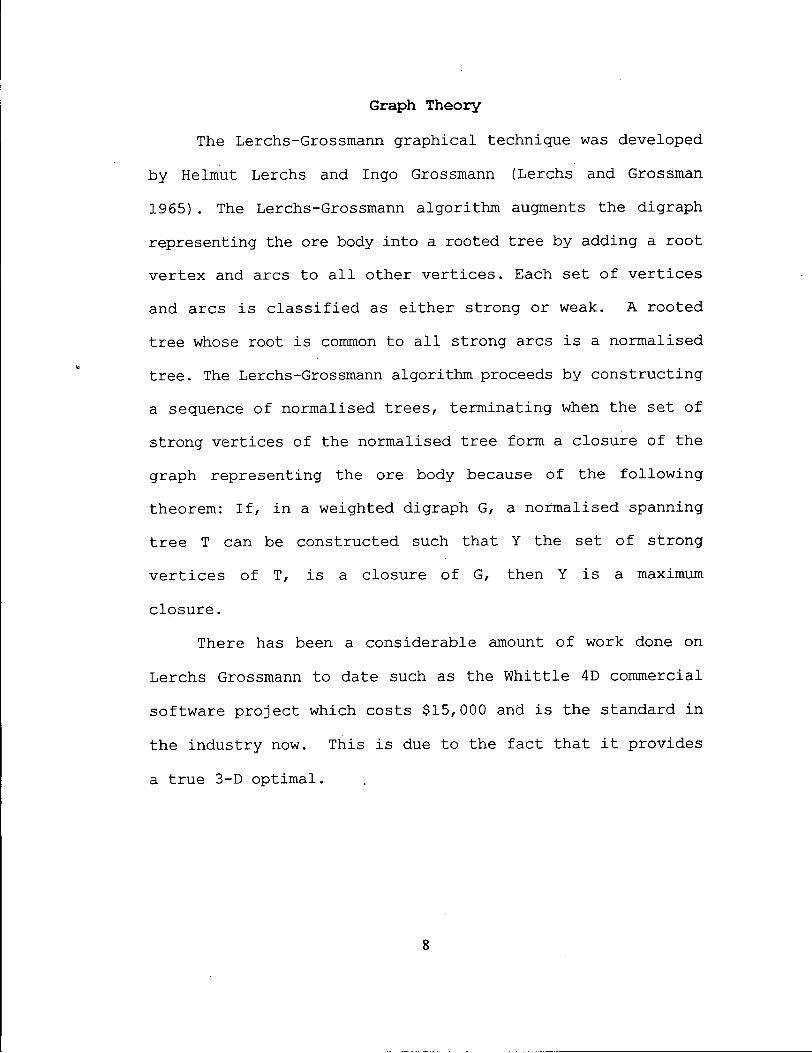
G r a p h T h e o r y

The Lerchs-Grossmann graphical technique was developed

by Helmut Lerchs and Ingo Grossmann (Lerchs and Grossman

1965). The Lerchs-Grossmann algorithm augments the digraph

representing the ore body into a rooted tree by adding a root

vertex and arcs to a l l other v e r t i c e s . Each set of v e r t i c e s

and arcs i s c l a s s i f i e d as e i t h e r strong or weak. A rooted

tree whose root i s common to a l l strong arcs i s a normalised

tree. The Lerchs-Grossmann algorithm proceeds by c o n s t r u c t i n g

a sequence of normalised trees, terminating when the set of

strong v e r t i c e s of the normalised tree form a closure of the

graph representing the ore body because of the f o l l o w i n g

theorem: I f , i n a weighted digraph G, a normalised spanning

t r e e T can be constructed such that Y the set of strong

v e r t i c e s of T, i s a closure of G, then Y i s a maximum

closure.

There has been a considerable amount of work done on

Lerchs Grossmann to date such as the W h i t t l e 4D commercial

software p r o j e c t which costs $15,000 and i s the standard i n

the i n d u s t r y now. This i s due to the f a c t that i t provides

a true 3-D optimal.

8

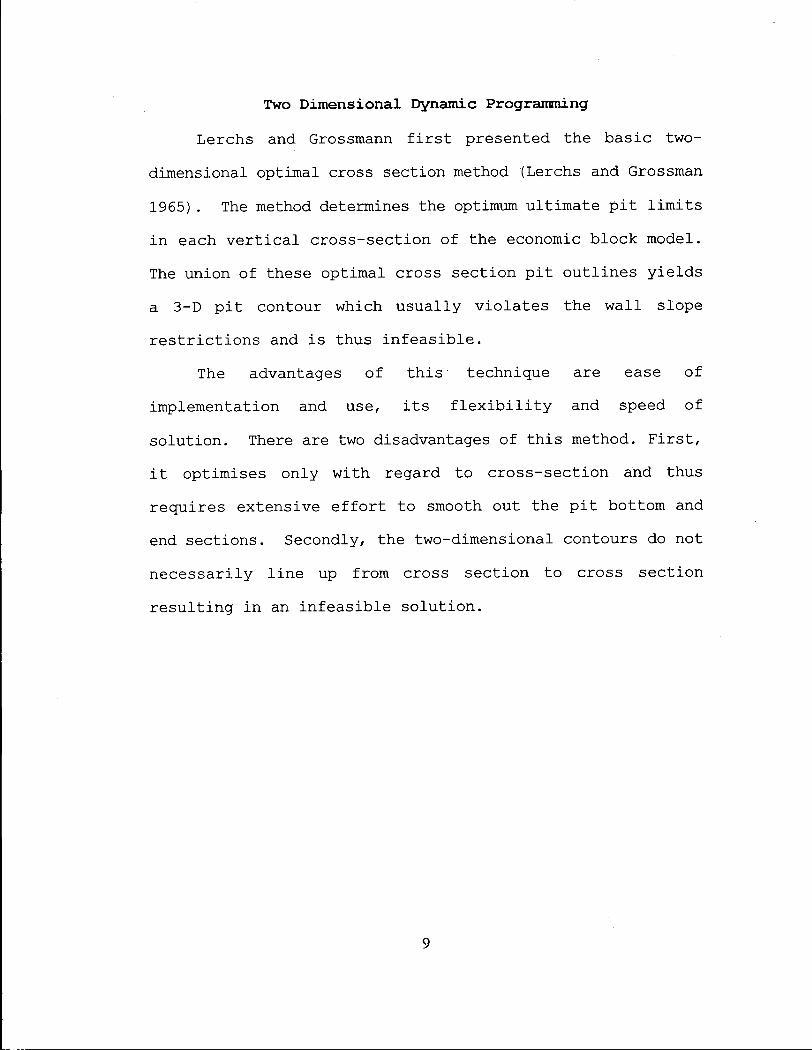
Two D i m e n s i o n a l D y n a m i c P r o g r a m m i n g

Lerchs and Grossmann f i r s t presented the b a s i c two-dimensional optimal cross section method (Lerchs and Grossman 1965) . The method determines the optimum ultimate p i t l i m i t s i n each v e r t i c a l c r o s s - s e c t i o n of the economic block model. The union of these optimal cross s e c t i o n p i t o u t l i n e s y i e l d s a 3-D p i t contour which u s u a l l y v i o l a t e s the w a l l slope r e s t r i c t i o n s and i s thus i n f e a s i b l e .

The advantages of t h i s technique are ease of implementation and use, i t s f l e x i b i l i t y and speed of sol u t i o n . There are two disadvantages of t h i s method. F i r s t , i t optimises only with regard to cr o s s - s e c t i o n and thus r e q u i r e s extensive e f f o r t to smooth out the p i t bottom and end sections. Secondly, the two-dimensional contours do not n e c e s s a r i l y l i n e up from cross s e c t i o n to cross s e c t i o n r e s u l t i n g i n an i n f e a s i b l e s o l u t i o n .

9

T h r e e D i m e n s i o n a l D y n a m i c P r o g r a m m i n g

A number of dynamic programming algorithms attempt to

extend the bas i c two-dimensional cross s e c t i o n routine

presented by Lerchs and Grossmann to handle the three-

dimensional problem. One such technique was developed by

Johnson and Sharp (1971). This technique eliminates the

bottom end smoothing which i s the primary disadvantage of the

two- dimensional technique.

The algorithm employs r e p e t i t i v e a p p l i c a t i o n of the

two-dimensional algorithm to obtain the optimum block

configuration on each cr o s s - s e c t i o n , f o r each l e v e l . Then a

f i n a l a p p l i c a t i o n of the two-dimensional algorithm on a

l o n g i t u d i n a l s e c t i o n where the blocks represent the optimal

s e c t i o n contours down to each l e v e l . There are two

advantages of the three-dimensional dynamic programming

technique. F i r s t l y , ease of understanding and implementation.

Secondly, f l e x i b i l i t y . The major disadvantage of t h i s method

i s that the s o l u t i o n may not be f e a s i b l e because the method

does not require adjacent c r o s s - s e c t i o n a l p i t configurations

to l i n e up. Other dynamic programming methods such as those

of Koenigsberg (1982) and B r a t i c e v i c (1984) seek to extend

the Johnson-Sharp method i n overcoming t h i s d i f f i c u l t y but

unfortunately r e s u l t i n s i g n i f i c a n t increases i n

computational complexity; s t i l l neither achieves a proper 3-D

10

optimum s o l u t i o n . A f u r t h e r disadvantage i s t h a t the 3-D

t e c h n i q u e w i l l not c o n s i d e r waste b l o c k s except those a l o n g

the two p r i n c i p a l axes o f the d e p o s i t ( c r o s s - s e c t i o n a l and

l o n g i t u d i n a l d i r e c t i o n s ) . The waste b l o c k s i n the c o r n e r

a rea o f the p i t are n e g l e c t e d i n d e v e l o p i n g the p i t l i m i t

optimum r e s u l t i n g i n s teeper p i t s l o p e s i n these a r e a s . T h i s

i s known as the corner e f f e c t .

11

L i n e a r P r o g r a m m i n g

I t i s natural, to formulate the open p i t problem as a

l i n e a r program since l i n e a r programming i s one of the most

popular operations research modelling techniques. The

formulation as a l i n e a r program i s very simple but the

so l u t i o n of such a model i s not computationally f e a s i b l e f o r

lar g e ore bodies. In order to apply l i n e a r programming

techniques the problem s i z e must be reduced.

12

N e t w o r k F l o w

Picard (1976) proposed a network flow model to solve

the maximum closure problem. The network N i s obtained from

the digraph D of the orebody by adding two vertices s

(source) and t (sink). The source i s joined to a l l vertices

having a positive weight by an arc of capacity equal to the

weight of the vertex. A l l vertices of negative weight are

joined to the sink by an arc having capacity equal to the

absolute value of the weight of the vertex. A l l the internal

arcs of D are given i n f i n i t e capacity. Picard formulated the

problem as a 0-1 program and showed that the maximal closure

of D corresponds to a minimal cut of N which can be found by

any of the standard maximum flow routines. There are a

number of algorithms to solve the maximum flow problem

(Ahuja, Magnanti, and Orlin) such as the network simplex

method of Dantzig, the augmenting path method of Ford-

Fulkerson, the blocking flow method of Dinic, and the push-

relabel method of Goldberg and Tarjan.

Network flow methods have been regarded by the mining

community as too slow and requiring too much memory, but this

was before good modern implementations. It i s not

theoretical bounds but run time that matters i n practice.

The empirical performance of push-relabel and Dinit's

algorithm are established i n a paper by Cherkassky and

13

Goldberg (1994). They implemented two versions of push-r e l a b e l (highest l a b e l and FIFO) each combined with g l o b a l and gap r e l a b e l i n g h e u r i s t i c s , and one implementation of D i n i c ' s algorithm. They ran these routines on randomly generated set of problems which were used at the F i r s t DIMACS Challenge (Cherkassky and Goldberg 1994). Their experiments show that both versions of push-relabel are e m p i r i c a l l y f a s t e r than D i n i t z f o r a l l set of problems and that the highest l a b e l version of push-relabel i s e m p i r i c a l l y f a s t e r than the FIFO versio n f o r a l l sets of problems. The performance of these routines on a c t u a l mining data i s i n v e s t i g a t e d i n t h i s t h e s i s . Some network flow techniques presented to date are discussed i n the f o l l o w i n g s e c t i o n s .

14

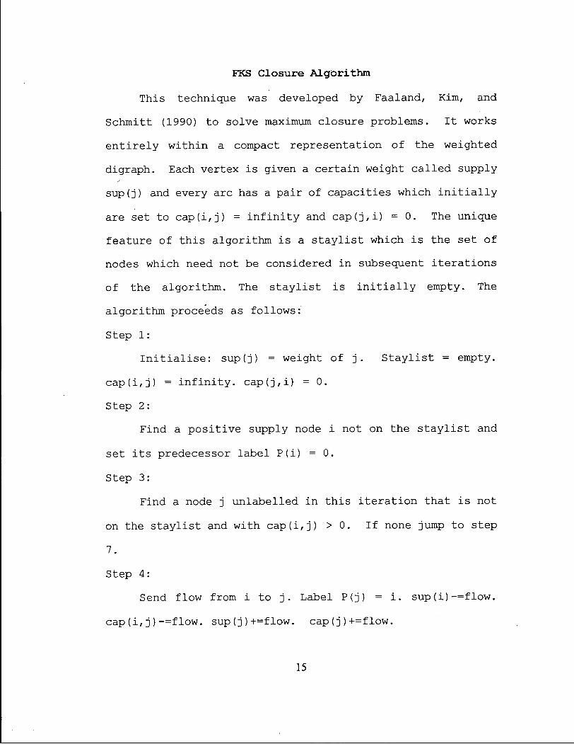
F K S C l o s u r e A l g o r i t h m

This technique was developed by Faaland, Kim, and

Schmitt (1990) to solve maximum closure problems. It works

en t i r e l y within a compact representation of the weighted

digraph. Each vertex i s given a certain weight c a l l e d supply

sup(j) and every arc has a pair of capacities which i n i t i a l l y

are set to cap(i,j) = i n f i n i t y and cap(j,i) = 0. The unique

feature of this algorithm i s a s t a y l i s t which i s the set of

nodes which need not be considered i n subsequent iterations

of the algorithm. The s t a y l i s t i s i n i t i a l l y empty. The

algorithm proceeds as follows:

Step 1:

I n i t i a l i s e : sup(j) = weight of j . S t a y l i s t = empty.

cap(i,j) = i n f i n i t y . cap(j,i) = 0.

Step 2:

Find a positive supply node i not on the s t a y l i s t and

set i t s predecessor label P(i) = 0.

Step 3:

Find a node j unlabelled i n this i t e r a t i o n that i s not

on the s t a y l i s t and with cap(i,j) > 0. If none jump to step

7.

Step 4:

Send flow from i to j . Label P(j) = i . sup (i) -=flow.

cap(i,j)-=flow. sup(j)+=flow. cap(j)+=flow.

15

Step 5:

If sup(j) > 0 then i = j go to step 2. Otherwise

sup(j) = 0 so backtrack to k=P(j).

Step 6:

If sup(k) > 0 then erase labels of j and nodes labelled

a f t e r j i n this i t e r a t i o n and set i=k and go to step 3.

Otherwise sup(k) = 0 so set j=k and go to step 5.

Step 7:

Backtrack from i to k=P(i).

Step 8:

If P(i) > 0 then send flow from i to k and reset sup

and cap and i=k and go to step 4. Otherwise P(i) =0 so add

i and nodes labelled after i to s t a y l i s t .

The maximum closure i n the digraph at the end of the

algorithm i s i d e n t i f i e d by the nodes i n the s t a y l i s t .

Faaland, Kim, and Schmitt's paper tests on small randomly

generated two-dimensional version of the open p i t problem

with this technique and so there i s no standard to compare

the empirical complexity of this algorithm with the others

stated above. We implemented this algorithm i n C to provide

a basis for the performance of push relabel and our

heu r i s t i c .

16

J o h n s o n ' s N e t w o r k F l o w

This technique was f i r s t proposed by Johnson i n 1968.

It uses the same block pattern representation of allowable

mining slopes as the Lerchs-Grossmann method and starts with

the same network representation of required allowable mining

sequence and converts i t into a b i p a r t i t e network. The

algorithm as i l l u s t r a t e d by Johnson (1973) proceeds as

follows:

Step 1:

We divide the blocks into two sets, (a) positive blocks

and (b) negative or zero blocks.

Step 2:

Connect each positive block to a l l negative blocks

which are required to be mined to remove the positive block

by adding arcs from the positive block to the negative block.

Step 3:

For each positive block allocate flow from the positive

block to i t s restricting negative blocks, mine this block and

i t s r e s t r i c t i n g blocks i f the sum i s positive. This process

usually requires reallocating flow for shared blocks i n the

network.

This technique leads to an optimal ultimate p i t l i m i t

but i t s disadvantage i s i t s in e f f i c i e n c y caused due to

reall o c a t i n g flow. The need to reallocate flow occurs when

17

r e s t r i c t i n g negative blocks are shared by positive blocks.

The reason i s that a uneconomic positive block should not be

used to support the stripping of an economic block which can

support i t s own stripping. This reallocation process has

been compared to the normalisation step i n the Lerchs-

Grossmann technique though Johnson's i s computationally less

expensive.

18

P u s h - R e l a b e l

Push-Relabel i s an algorithm for finding a maximum flow

through a network. A flow network i s a directed graph G =

(V,E ,S/t,u) where V and E are the node and arc set. Nodes s

and t are the source and the sink and u i s the nonnegative

capacity on the arcs. A flow i s a function that s a t i s f i e s

capacity constraints on a l l arcs and conservation constraints

on a l l nodes except the source and the sink. The

conservation constraint at a node v states that the excess

e(v), defined as the difference between the incoming and the

outgoing flows, i s equal to zero. A preflow s a t i s f i e s the

capacity constraints and the relaxed conservation constraints

that only require the excesses to be nonnegative.

An arc i s residual i f the flow on i t can be increased

without v i o l a t i n g the capacity constraints, and saturated

otherwise. The residual capacity of an arc i s the amount by

which the arc flow can be increased. A distance l a b e l l i n g

d:V-> N s a t i s f i e s the following conditions: d(t) =0 and for

every residual arc (v,w), d(v) <= d(w) + 1. A residual arc

(v,w) i s admissible i f d(v) = d(w) + 1. A node v i s active

i f d(v) < n and e(v) > 0.

The push-relabel algorithm maintains a preflow and a

distance labelling t i l l there are no active nodes. Then the

preflow i s converted to a flow. The push relabel routines of

19

Cherkassky and Goldberg (1994) proceed as follows:

Step 1:

Find an active node v. An active node i s one with

positive excess and distance label less than n. If there are

no active nodes then stop.

Step 2:

Find the next edge (v,w) of v. If none go to step 4.

Step 3:

If(v,w) i s admissible then send d = (0,min(excess(v) ,

residual capacity(v, w)) units of flow from v to w and repeat

step 3 u n t i l excess(v) equal zero. If (v,w) not admissible go

to step 2.

Step 4:

Replace v's distance label d(v) by min(ViW)d(w) + 1. Go

to step 1.

The main discharge operation i s applied i t e r a t i v e l y to

active nodes as above. A l l that i s l e f t i s to decide the

order i n which these active nodes must be processed. There

are two alternatives presented by Goldberg and Cherkassky.

The f i r s t one i s known as the FIFO algorithm and maintains

a l l active nodes i n a queue adding active nodes to the rear

of the queue and discharging positive nodes from the front of

the queue i n a F i r s t - I n First-Out order. The second one i s

the HL algorithm and always selects the node with the highest

20

label to discharge f i r s t . Cherkassky and Goldberg improve the

p r a c t i c a l performance of the push relabel algorithms by

adding global and gap r e l a b e l l i n g heuristics to the maximal

flow code. In their paper (1994) Cherkassky and Goldberg

show that both the push relabel routines perform better than

Dinitz on randomly generated sets of data from the DIMACS

generators.

21

H e u r i s t i c M e t h o d s

Although a number of heuristic methods have been

proposed, only one of them has been widely accepted, the

f l o a t i n g cone. The method's wide acceptance stems from the

fact that i t very easily understood and easy to program.

Also, there i s no re s t r i c t i o n on wall slope v a r i a b i l i t y . The

method as i l l u s t r a t e d by Johnson (1973) proceeds as follows:

Step 1:

Define a certain potential mining volume by stating a

bottom block and the allowable wall slopes.

Step 2:

Sum the value of a l l the blocks whose centres l i e

inside the defined cone.

Step 3:

Select the cone for mining i f the t o t a l value i s

greater than zero.

The above process i s continued u n t i l i t i s not possible

to find any cones of positive value. The advantages of this

technique are that i t i s e a s i l y to understand, allows

variable p i t slopes, i s easy to implement, and that variable

size blocks present no d i f f i c u l t y . The basic shortcoming of

the method i s i t s i n a b i l i t y to consider j o i n t contributions

of multiple ore blocks located l a t e r a l l y a distance apart

thereby missing the optimal solution.

22

C H A P T E R 4

O u r I m p l e m e n t a t i o n

As described earlier, the open p i t l i m i t problem can be

converted to a maximum flow problem. The maximum flow

problem i s very easy to state: In a capacitated network, we

want to send as much flow as possible between two nodes

c a l l e d the source s and the sink t, without v i o l a t i n g the

capacity r e s t r i c t i o n on any arc. There are a number of

algorithms for solving the maximal flow problem. As

mentioned i n Chapter 3, the basic methods are:

(1) Network simplex method of Dantzig

(2) The Augmenting Path method of Ford and Fulkerson

(3) The Blocking Flow method of Dinic

(4) Push Relabel method of Goldberg and Tarjan

Studies by Goldfarb and Grigoriadis (1988) showed that

Dinitz algorithm i s i n practice superior to the network

simplex and the Ford-Fulkerson methods. Several recent

studies such as those by Anderson and Setubal (1993) and

Nguyen and Venkateswaran (1993) show that the push relabel

method i s superior to Dinic's method i n practice. In

particular the paper by Goldberg and Cherkassky (1994) showed

that two versions of push relabel perform better than Dinitz

for a l l problem sets generated by the First DIMACS challenge;

The data used to come to this conclusion are randomly

23

generated by the DIMACS network generators. This thesis

attempts to confirm these conclusions on real sets of data

for open-pit mining problems.

Tom McCormick and Todd Stewart's code generates a

bounded network with a minimum possible number of blocks and

arcs. I imbed several implementations of heuristics as the

network i s generated to check i f we can improve the

performance of push relabel by giving i t a "warm sta r t " .

Since the push-relabel deals with preflows one can, greedily

or by taking advantage of a open p i t mine structure, push as

much flow as we want and input these excesses as a preflow

into the push-relabel routine thereby giving i t a warm star t .

F i r s t l y , the network generation routine establishes the

lowest positive value block i n each row column pair of the

ore body because there i s no need to consider any blocks

beneath these. Next we have to add on those blocks that are

outside the ore body that would need to be removed i n order

to remove blocks within the ore body. This i s given by the

.spp f i l e which i s the cone of slopes of azimuths above any

block. The .spp f i l e gives us a l l the blocks that need to be

removed i n order to remove a specific block. F i n a l l y , we also

have to add on blocks that are necessary to s a t i s f y wall

slope r e s t r i c t i o n . This i s given by the .spv f i l e which

gives the minimum set of arcs whose tra n s i t i v e closure gives

24

the same cone given by the .spp f i l e . The .spv f i l e gives us

the outer boundary blocks of the .spp f i l e . The .spp and

.spv f i l e s are generated v i a Lynx's code and examples of

these f i l e s are given on pages 47 and 52.

We attempt to enhance the speed of the network flow

routine by giving i t a warm start. Several heuristics are

studied i n order to take advantage of the three dimensional

structure of the open p i t mine network that i s solved by a

generic maximum flow problem. The network generator proceeds

as follows:

Step 1:

Read i n the 3-D block array with block values.

Step 2:

Establish a bottom layer for each row-column pair as

the lowest positive block layer.

Step 3:

Extend the bottom array to a new bottom whose size i s

expanded as indicated by the .spp f i l e to allow blocks

outside the o r i g i n a l orebody to be mined.

Step 4:

Establish a linked l i s t of a l l positive value bottom

layers.

Step 5: Run through this linked l i s t and add any new bottom

25

layers that are needed as indicated by the .spp f i l e to

s a t i s f y wall slope requirements.

Step 6:

Number a l l the blocks that are i n the network.

Step 7:

Run through each block from bottom up generating the

minimum possible number of arcs needed to remove that block

as given by the .spv f i l e . Attempt to push flow as dictated

by the heu r i s t i c .

26

V A R I O U S H E U R I S T I C S

We are using a generalised maximum flow routine (push

relabel) to solve a sp e c i f i c application which i s the open

p i t mine problem. The open p i t mine problem has a three

dimensional structure and f i n i t e capacities on source and

sink arcs only. The idea then i s to use this special

structure to enhance the performance of the push relabel

routine. Various heuristics are implemented and incorporated

into the network generation routine, and give the push

re l a b e l routine a warm start. The performance of each

h e u r i s t i c i s judged by the percentage reduction i n solution

time of the push relabel routine over three instances of

networks chosen to show a range of performance of the

he u r i s t i c s . The three networks are generated from the

blockmod data which i s a r t i f i c i a l l y generated to represent

a real mine. There are two classes of heuri s t i c s . F i r s t l y ,

those that push flow using arc information only. Secondly

those that push flow using node information also.

C l a s s 1

M I N I M U M l x

We know that i n order to remove blocks on one layer we

need to remove blocks from the layers above this layer. The

way the network i s generated the ore body generally l i e s i n

the central (row,column) area. Therefore we expect the

27

central blocks i n the upper layer to be i n the optimal

solution. The f i r s t and most obvious heur i s t i c we consider

i s based on the minimum lx distance. Each arc has a t a i l ,

head pair. The difference between the t a i l ' s row number and

the head's row number i s the row offset of t h i s arc.

S i m i l a r l y we have a column and a layer o f f s e t . The lx

distance i s then defined as the row offset plus the column

of f s e t . The l x norm i s the sum of the absolute values of

offsets. So a smaller lx distance means an arc that goes up

straight for and a smaller l a t e r a l deviation. Therefore we

want to push flow on minimum l x distance arcs since they push

flow straight up straying the least from the central blocks.

This i s accomplished through creating an array of

linked l i s t s where the array index equals the l x distance of

the arc. Then a l l arcs with the same lx distance are part of

one linked l i s t so each time an arc i s generated we push flow

f i r s t to the sink i f possible, and then to arcs beginning

from minimum l a distance linked l i s t to increasing 1

distance linked l i s t s a l tering the excess on the respective

nodes and the flow on the arcs.

The mean solution times with and without the h e u r i s t i c

are shown below for the representative set of networks.

28

Network

a60

b45

c50

Nodes

2813

4277

4097

Heuristic

.55

1.12

1.78

Push-Rel

. 63

1.23

1.8

Reduction

13 %

9 %

1 %

M A X I M U M Z

We define the z distance of any arc as z =layer of f s e t .

We push flows on arcs i n order of decreasing layer o f f s e t .

Arcs connected to higher layers get flow f i r s t with the

exception of arcs to the sink getting flow f i r s t . Here we do

not care i f flow i s moving away from the central (row, column)

blocks as long as i t s going up as fast as possible. The

performance of this heuristic was tested on blockmod and a

sample follows:

Network Nodes Heuristic Push-Rel Reduction

a60 2813 .57 .63 10 %

b45 4277 1.20 1.23 2 %

c50 4097 1.8 1.8 0 %

M A X I M U M l x

We know that before any block i s i n the optimal

solution i t s value must be greater than the value of the head

of any of i t s arcs not considering the combined flow effect

from other nodes. The central nodes are more l i k e l y to get

29

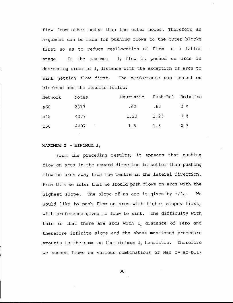
flow from other nodes than the outer nodes. Therefore an

argument can be made for pushing flows to the outer blocks

f i r s t so as to reduce reallocation of flows at a l a t t e r

stage. In the maximum lx flow i s pushed on arcs i n

decreasing order of l x distance with the exception of arcs to

sink getting flow f i r s t . The performance was tested on

blockmod and the results follow:


a60 2813 .62 .63 2 %

b45 4277 1.23 1.23 0 %

c50 4097 1.8 1.8 0 %

M A X I M U M Z - M I N I M U M l x

From the preceding results, i t appears that pushing

flow on arcs i n the upward direction i s better than pushing

flow on arcs away from the centre i n the l a t e r a l direction.

From this we infer that we should push flows on arcs with the

highest slope. The slope of an arc i s given by z/l1. We

would l i k e to push flow on arcs with higher slopes f i r s t ,

with preference given to flow to sink. The d i f f i c u l t y with

t h i s i s that there are arcs with l x distance of zero and

therefore i n f i n i t e slope and the above mentioned procedure

amounts to the same as the minimum l x h e u r i s t i c . Therefore

we pushed flows on various combinations of Max f=(az-bll)

30

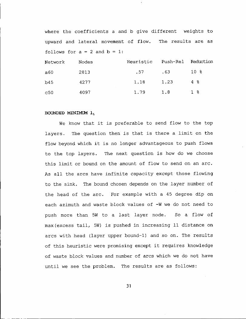
where the coefficients a and b give different weights to

upward and l a t e r a l movement of flow. The results are as

follows for a = 2 and b = 1:


a60 2813 .57 .63 10 %

b45 4277 1.18 1.23 4 %

c50 4097 1.79 1.8 1 %

B O U N D E D M I N I M U M l x

We know that i t i s preferable to send flow to the top

layers. The question then i s that i s there a l i m i t on the

flow beyond which i t i s no longer advantageous to push flows

to the top layers. The next question i s how do we choose

this l i m i t or bound on the amount of flow to send on an arc.

As a l l the arcs have i n f i n i t e capacity except those flowing

to the sink. The bound chosen depends on the layer number of

the head of the arc. For example with a 45 degree dip on

each azimuth and waste block values of -W we do not need to

push more than 5W to a l a s t layer node. So a flow of

max(excess t a i l , 5W) i s pushed i n increasing 11 distance on

arcs with head (layer upper bound-1) and so on. The results

of this heuristic were promising except i t requires knowledge

of waste block values and number of arcs which we do not have

u n t i l we see the problem. The results are as follows:

31


a60 2813 .55 .63 13 %

b45 4277 1.10 1.23 11 %

c50 4097 1.78 1.8 1 %

N O FLOWS I N K

For each of the heuristic above, we prefer to send flow

to the sink f i r s t and then to the arcs indicated by the

h e u r i s t i c . It i s only natural to try what happens i f we

avoid any arcs flowing to the sink rather than prefer them.

The performance with minimum l x h e u r i s t i c was tested on

blockmod and the results were as follows:


a60 2813 .65 .63 -3 %

b45 4277 1.26 1.23 -2 %

c50 4097 1.83 1.8 -2 %

C L A S S 2

We have been considering just the characteristics of

the arc without considering any information on the nodes.

The next set of heuristics use information about both arcs

and nodes. From now on, we push on arcs with minimum lt

distance giving preference to flow to sink since this was the

best heuristic but we also apply information from the nodes.

32

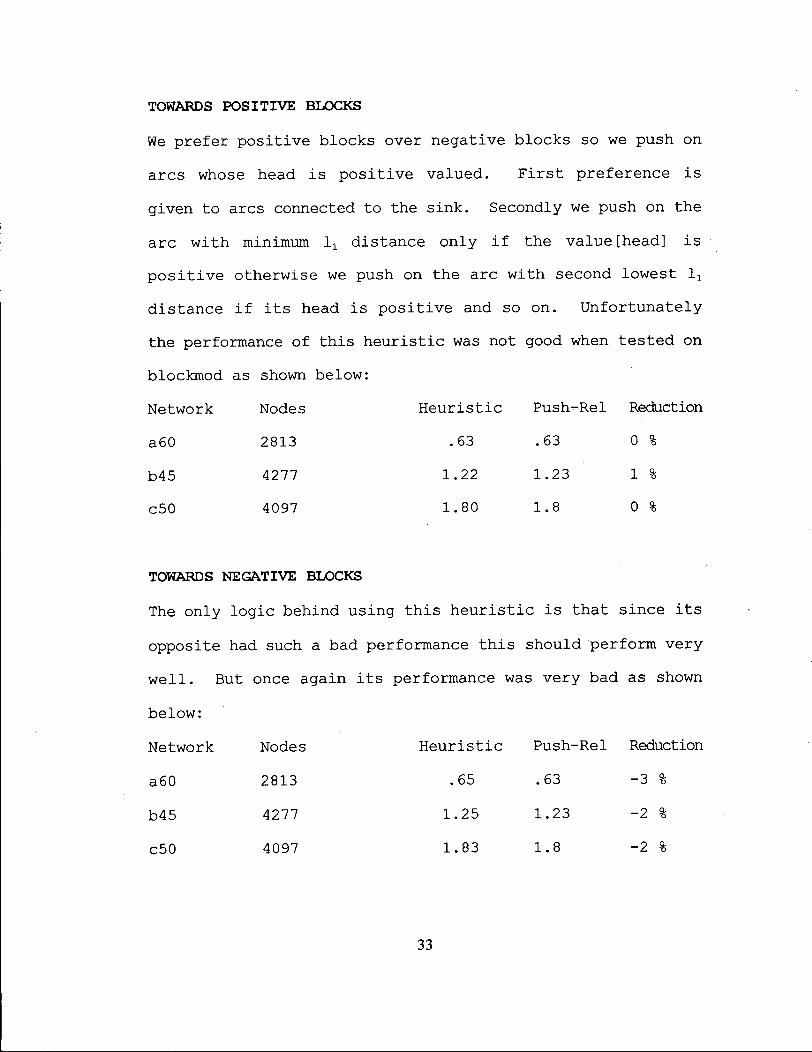
TOWARDS P O S I T I V E B L O C K S

We prefer positive blocks over negative blocks so we push on

arcs whose head i s positive valued. F i r s t preference i s

given to arcs connected to the sink. Secondly we push on the

arc with minimum lx distance only i f the value [head] i s

po s i t i v e otherwise we push on the arc with second lowest lr

distance i f i t s head i s positive and so on. Unfortunately

the performance of this heuristic was not good when tested on

blockmod as shown below:


a60 2813 .63 .63 0 %

b45 4277 1.22 1.23 1 %

c50 4097 1.80 1.8 0 %

TOWARDS N E G A T I V E B L O C K S

The only logic behind using this h e u r i s t i c i s that since i t s

opposite had such a bad performance this should perform very

well. But once again i t s performance was very bad as shown

below:


a60 2813 .65 .63 -3 %

b45 4277 1.25 1.23 -2 %

c50 4097 1.83 1.8 -2 %

33

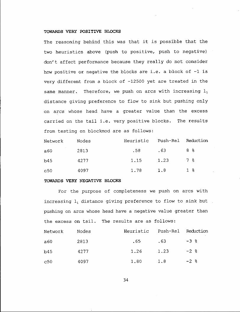
TOWARDS V E R Y P O S I T I V E B L O C K S

The reasoning behind this was that i t i s possible that the

two heuristics above (push to positive, push to negative)

don't affect performance because they r e a l l y do not consider

how positive or negative the blocks are i.e. a block of -1 i s

very different from a block of -12500 yet are treated i n the

same manner. Therefore, we push on arcs with increasing 11

distance giving preference to flow to sink but pushing only

on arcs whose head have a greater value than the excess

carried on the t a i l i . e . very positive blocks. The results

from testing on blockmod are as follows:


a60 2813 .58 .63 8 %

b45 4277 1.15 1.23 7 %

c50 4097 1.78 1.8 1 %

TOWARDS V E R Y N E G A T I V E B L O C K S

For the purpose of completeness we push on arcs with

increasing 11 distance giving preference to flow to sink but

pushing on arcs whose head have a negative value greater than

the excess on t a i l . The results are as follows:


a60 2813 .65 .63 -3 %

b45 4277 1.26 1.23 -2 %

c50 4097 1.80 1.8 -2 %

34

A N A L Y S I S & C O N C L U S I O N

The average (over the sample size of three) reduction

in solution time for a l l the heuristics i s as follows. Other

tests similar to these were done on sab02 confirming these

results but s t i l l the sample size i s small and the number of

base instances (2) i s also small.

(1) Bounded minimum 11 8%

(2) Minimum l x 8%

(3) Maximum z - minimum l a 5%

(4) Very positive 5%

(5) Maximum z 4%

(6) Maximum lt 1%

(7) Positive 0%

(8) Negative -2%

(9) Very negative -2%

(10) No flowsink -2%

The heuristics with the greatest percentage reduction

in mean solution time are bounded minimum l x and minimum 1}.

The extra information required to run bounded minimum lx does

not lead to a significant reduction i n solution time. Also,

the bounded value for flow i s problem s p e c i f i c and requires

knowledge of the waste block values and .spv f i l e s

beforehand.

The inherent v a r i a b i l i t y i n solution times i s very

35

l i t t l e (i.e. .02 seconds at the most for a l l heuristics) . The

difference in solution times of these two heuristics and push

relabel are strongly s t a t i s t i c a l l y s i g n i f i c a n t . As mentioned

before we do suffer from a lack of more base instances (sab02

and blockmod) but an attempt was made to generate networks

that are as different as possible. This i s further discussed

in Chapter 5.

On the basis of these runs the minimum lx h e u r i s t i c was

adopted. The output from the network flow generator

(incorporated with the minimum l x heuristic) i s now read into

a parser and maximal flow routines. The parser routine must

be altered to read an extended format which i s required for

reading i n the output of the heuristic i n order to give the

maximal flow routine a warm start.

The output from the parser i s read into Cherkassky and

Goldberg's (1994) push relabel routines with changes made to

incorporate the warm start. The networks are run on two

maximum flow routines with and without the he u r i s t i c . The

same networks are run on Dinic's algorithm without the warm

start and our implementation of FKS (chapter 2) to provide a

basis for comparison with push relabel.

36

I l l u s t r a t i v e e x a m p l e

We consider a small problem to i l l u s t r a t e the steps

that the minimum l x heuristic incorporated network generation

routine runs through. The problem we consider has three

rows, three columns, and three layers. So the o r i g i n a l ore

body three dimensional block structure has twenty seven

blocks. Let's consider the ore body f i r s t :

Layer 1 (Bottom layer)

-1 -1 -1 -1 -1 -1 10 -1 10

Layer 2

-1 -1 8 -1 -1 -1 -1 -1 8

Layer 3

-1 -1 -1 -1 -1 -1 -1 -1 -1

The 3*3*3 ore body model i s read into the routine. For

example, the value of block row 1, column 3, and layer 2 i s

8. The next step i s to find the lowest positive layer i n

each row-column pair and put i t i n a two dimensional array

bottom[i] [j] = value. If there i s no positive layer then i t s

value i s set to M.

37

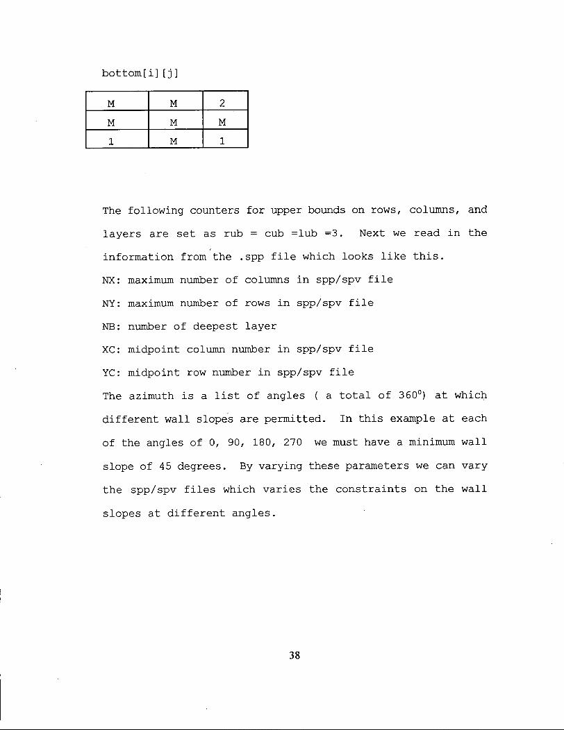
bottom[i] [j]

M M 2 M M M 1 M 1

The following counters for upper bounds on rows, columns, and

layers are set as rub = cub =lub =3. Next we read i n the

information from the .spp f i l e which looks l i k e t h i s .

NX: maximum number of columns i n spp/spv f i l e

NY: maximum number of rows i n spp/spv f i l e

NB: number of deepest layer

XC: midpoint column number i n spp/spv f i l e

YC: midpoint row number i n spp/spv f i l e

The azimuth i s a l i s t of angles ( a t o t a l of 360°) at which

different wall slopes are permitted. In this example at each

of the angles of 0, 90, 180, 270 we must have a minimum wall

slope of 45 degrees. By varying these parameters we can vary

the spp/spv f i l e s which varies the constraints on the wall

slopes at different angles.

38

NX, NY, NB, XC, YC, NP, BX, BY, BH= 7 7 3 4 4 4 10 10 10 AZIMUTH = .0 90.0 180.0 270.0 DIP = 45.0 45.0 45.0 45.0 001:00000003000000 002:00030302030300 003:00030201020300 004:03020101010203 005:00030201020300 006:00030302030300 007:00000003000000

After reading the spp f i l e we create an expanded bottom

array bottom[i] [j] to allow for mining of blocks outside the

ore body i n order to remove blocks at the edges of the ore

body three dimensional blocks. It i s the size of this block

structure which represents the number of blocks we would have

i n our model i f we did not have a bounding routine which i n

this case would be 7*7*3=142. The new bottom array w i l l have

dimensions equal to old dimensions + (NX,NY) which means

(7,7). The information from the old bottom i s transferred to

the new bottom array as (row=row + NY/2) and (column=column

+ NX/2).

new bottom[i] [j]

M M M M M M M M M M M M M M M M M M 2 M M M M M M M M M M M 1 M 1 M M M M M M M M M M M M M M M M

39

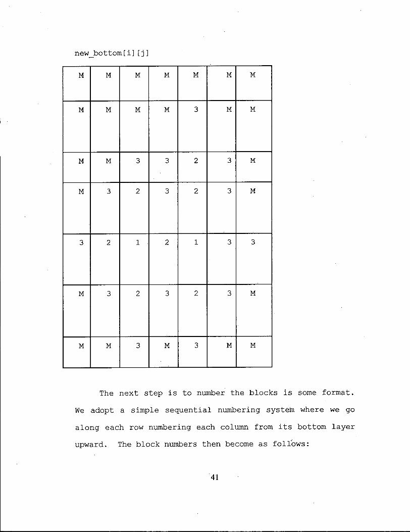
Next we construct a linked l i s t of each non-M bottom

row-column pair for each l e v e l . For example our linked l i s t

for layer 1 would contain two elements and their respective

row-column pairs and for layer 2 we have one element and i t s

row-column pair. We then run through our linked l i s t and

apply the information available i n the spp f i l e by putting

i t s centre (4,4) over each block i n the linked l i s t to find

out what blocks need to be added to s a t i s f y the wall slope

r e s t r i c t i o n s . If any blocks are needed then we have to

create new bottom blocks for that row-column pair. So we get

an updated new_bottom[i][j].

40

new bottom[i][j]

M M M M M M M

M M M M 3 M M

M M 3 3 2 3 M

M 3 2 3 2 3 M

3 2 1 2 1 3 3

M 3 2 3 2 3 M

M M 3 M 3 M M

The next step i s to number the blocks i s some format.

We adopt a simple sequential numbering system where we go

along each row numbering each column from i t s bottom layer

upward. The block numbers then become as follows:

41

36 31 32 34,

33

35

24 26,

25

27 29,

28

30

10 12, 15, 17, 20, 22, 23

11 14,

13

16 19,

18

21

3 5

4

6 8

7

9

1 2

So our bounding structure uses a t o t a l of 36 blocks as

opposed to an o r i g i n a l number of 142 blocks. We can now

pri n t out each block and i t s value to the output f i l e . A l l

blocks outside the o r i g i n a l ore body can be given any value.

In this example they are given a value of -1.

42

We now input information form the .spv f i l e which looks

l i k e this

NX, NY, NB, XC, YC, NP, BX, BY, BH= 7 7 3 4 4 4 10 10 10 AZIMUTH = .0 90.0 180.0 270.0 DIP = 45.0 45.0 45.0 45.0 001:00000000000000 002:00030000000300 003:00000001000000 004:00000101010000 005:00000001000000 006:00030000000300 007:00000000000000

We use this f i l e to set up the arcs. By placing the centre

(4,4) over each block we can set up the arcs that lead out

from each block. In general, the order i n which you generate

these arcs doesn't matter. In our case we want to set up a

heuristic which pushes flow as i t generates the arcs on arcs

of increasing l x distance so that we can . Consequently, we

must generate these arcs according to ascending 11 distance.

We read each nonzero value from the spp f i l e and assign

i t a row offset and a column offset number. Then we create

an array of linked l i s t s where the array index equals the 12

distance of each nonnegative value i n the spp f i l e . Now we

can generate arcs by running through the linked l i s t of each

the array i n ascending order of the array index.

For example, from the spp f i l e above the entry i n (4,4) has

l x distance 0 and so i s the f i r s t member of the linked l i s t

of the array element b[0] . Similarly we have four members i n

43

the linked l i s t of array element b[l] with lx distance 1 i . e .

(5,4), (4,5), (4,3), (3,4).

In order to run the heuristic we need to assign excess

on blocks and flows on arcs as we generate the arcs. A l l

pos i t i v e value blocks are assigned an excess equal to th e i r

value and the rest of the blocks have zero excess to start

with.

Once the heuristic i s done we output each arc and i t s

flow and each block and i t s excess and i t s flow to the sink.

The heuristic has pushed excess to the top layers i n order to

give the maximal flow routine a warm star t . This output i s

now read into the parser and the modified maximal flow

routines.

We see that our bounding procedure resulted i n

decreasing the number of blocks from 142 to 36 and the

he u r i s t i c has pushed excess to the upper levels i n order to

give the maximal flow routine a warm start.

44

C H A P T E R 5

R e s u l t s

The usefulness of any technique cannot be measured

u n t i l i t i s applied to an actual problem. We use the data

from a Brazilian copper mine (sab02) and data constructed to

resemble a real mine (blockmod) to address the following

issues:

1) Whether the push relabel routine works well i n practice on

this class of graphs.

2) Whether we can take advantage of the structure of an open

p i t problem being solved with a generic maximum flow code.

3) To what extent does the network generation procedure

reduce the number of blocks.

These questions are answered using both a small example

and real mine deposit data. The Brazilian copper mine(sab02)

has 23 layers, 52 rows, and 80 columns for a t o t a l of 95680

blocks. The small example (blockmod) has 12 layers, 11 rows,

and 23 columns for a t o t a l of 3036 blocks. We use these two

data sets to generate a number of different networks to do

our testing. We were limited to only these two base

instances of which r e a l l y only one i s actual data, and the

other i s small and a r t i f i c i a l . Ideally i t would be better to

have more base instances. Consequently we generated the

networks to be as different as possible from each other. The

45

networks generated through different .spp and .spv f i l e s

range from 2813 to 27926 nodes. We run our routines on a

HP/Apollo 9000, model 730 with 64 MB RAM with a GNU C

compiler and the implementations are written i n C.

We have tested on 4 different routines which are

(1) The FKS closure algorithm which we implemented i n C.

(2) Dinic's algorithm as implemented by Goldberg and

Cherkassky (1990).

(3) The queue push relabel implementation of Goldberg and

Cherkassky.

(4) The highest label push relabel implementation of Goldberg

and Cherkassky.

We implemented the minimum 11 h e u r i s t i c which we

incorporated into Tom McCormick and Todd Stewart's network

generator and implemented a parser routine i n order to

incorporate the warm start into both push relabel routines.

S o l u t i o n T i m e ( P u s h R e l a b e l )

Goldberg and Cherkassky (1994) show that the empirical

performance for both push relabel routines ( highest label

and FIFO ) i s better than Dinic's. Their paper also

establishes that the highest label push relabel

implementation performs better than the FIFO push relabel

routine for a l l random problem sets. Goldberg and Cherkassky

46

perform their tests on randomly generated data from the f i r s t

DIMACS challenge. The empirical performance of the push

relabel on actual data has not been tested as far as we know.

Therefore we run a l l five routines on real data (sab02) and

generated data (blockmod) to v e r i f y the empirical properties

established by Goldberg and Cherkassky. Table One gives the

solution times over a l l tested networks respectively for FKS,

Dinics, Push Relabel (FIFO), Push Relabel (FIFO) plus minimum

l x heuristic, Push Relabel (Highest Label), and Push Relabel

(Highest Label) plus minimum 12 h e u r i s t i c . Figure One plots

the solution times for FKS, Dinic's, and Push Relabel (FIFO),

Push Relabel (FIFO) plus heuristic for both sets of data

(sab02 and blockmod) together and separately. Figure Two

plots the same solution times from Figure One except for FKS

i n order to better scale the graph since FKS times are much

larger than the other routines. Figure Three plots the

solution times for FKS, Dinic's, Push Relabel (Highest Label)

and Push Relabel (Highest Label) plus heuristic for both sets

of data (sab02 and blockmod) together and separately. Figure

Four plots these solution times i n Figure Three except for

FKS i n order to scale the graph.

The results from testing on actual data confirm those

of Cherkassky and Goldberg (1994) on randomly generated data.

The highest label push relabel implementation i s the fastest

47

followed by FIFO push relabel and then Dinic's. Our

implementation of FKS was the slowest.

S o l u t i o n T i m e ( H e u r i s t i c )

The push relabel incorporated with minimum l x h e u r i s t i c

performs better than just the push relabel for both routines.

Each routine i s run on the same network many times to check

i f the difference i n solution times i s s t a t i s t i c a l l y

significant. The solution and to t a l times i n CPU seconds for

three networks (A45, B45, and C60) are shown with the t-

s t a t i s t i c for difference i n mean solution time.

Heuristic Push Relabel A45 FIFO

Total Solution Total Solution 1 62.98 19.17 63.65 20.88 2 64.62 19.82 63.48 20.90 3 63.02 19.17 63.42 20.88 4 63.00 19.07 63.18 20.80 5 63.23 19.15 63.67 20.88 6 63.62 19.17 64.03 20.95 t = -14.10 P = .0000 B45 FIFO

Total Solution Total Solution 1 89.17 26.43 91.17 28.40 2 88.72 26.43 89.70 28.35 3 89.33 26.40 89.07 28.28 4 88.87 26.45 89.05 28.40 5 89.45 26.43 89.93 28.40 6 89.17 26.43 89.82 28.35 t = -94.36 P = .0000 A45 Highest Label

Total Solution Total Solution 1 58.48 14.47 58.50 15.78 2 58.55 14.45 58.68 .15.77 3 58. 67 14.40 58.58 15.73 4 61.10 14.42 65.15 15.88 5 58.55 14.50 58.70 15.82 6 58. 67 14.50 58.73 15.80 t = -50.09 P - .0000

48

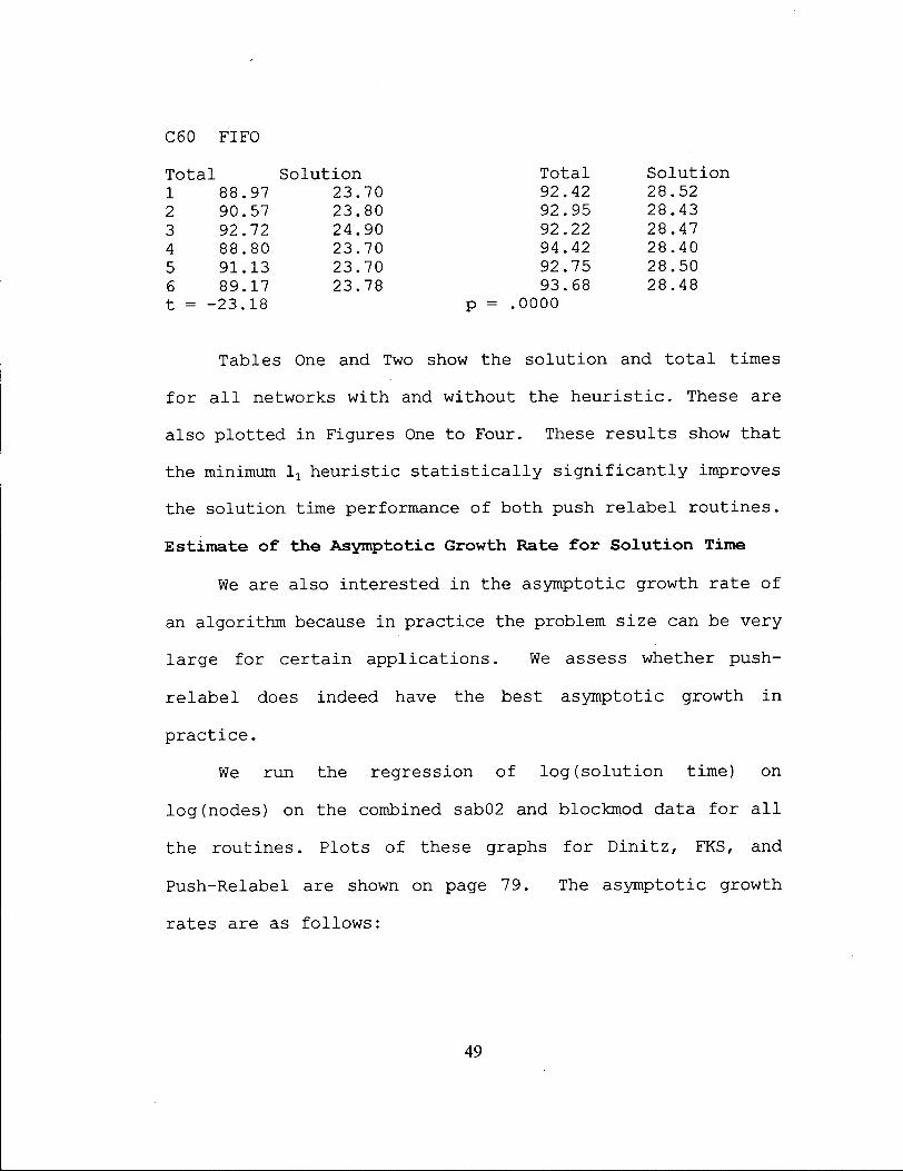
C60 FIFO

Total Solution Total 92.42 92.95 92.22 94.42 92.75 93.68

Solution 1 88.97 2 90.57 3 92.72 4 88.80 5 91.13 6 89.17 t = -23.18

23.70 23.80 24.90 23.70 23.70 23.78

28.52 28.43 28.47 28.40 28.50 28.48

p = .0000

Tables One and Two show the solution and t o t a l times

for a l l networks with and without the he u r i s t i c . These are

also plotted in Figures One to Four. These results show that

the minimum l x heuristic s t a t i s t i c a l l y s i g n i f i c a n t l y improves

the solution time performance of both push relabel routines.

E s t i m a t e o f t h e A s y m p t o t i c G r o w t h R a t e f o r S o l u t i o n T i m e

We are also interested i n the asymptotic growth rate of

an algorithm because in practice the problem size can be very

large for certain applications. We assess whether push-

re l a b e l does indeed have the best asymptotic growth i n

practice.

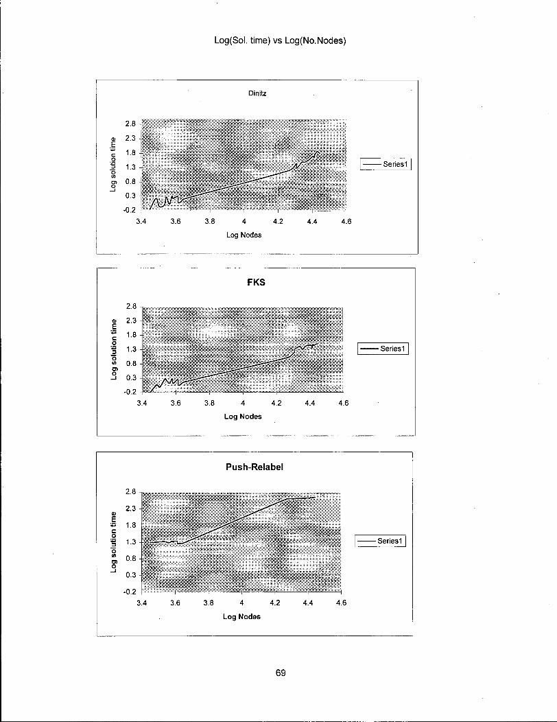
We run the regression of log(solution time) on

log(nodes) on the combined sab02 and blockmod data for a l l

the routines. Plots of these graphs for Dinitz, FKS, and

Push-Relabel are shown on page 79. The asymptotic growth

rates are as follows:

49

FKS 1.58

Dinic 1.82

PR(Q) 1.54

PR(Q)+H 1.53

PR(H) 1.51

PR(H)+H 1.50 ,

The push relabel algorithm has a better asymptotic

growth rate for this class of real problems implying that as

the problem size increases the performance of push relabel

improves even further. This i l l u s t r a t e s how well the push

relabel routine performs i n practice on actual data.

T o t a l t i m e

It i s plausible that we might be concerned about the

total time taken to read the network, solve the maximum flow

problem and output the maximum closure. We see the t o t a l and

solution times for each of the routines in Tables 3, 4, 5, 6,

7, 8 respectively. Also Figure 5 plots the to t a l time for a l l

routines.

The most s t r i k i n g thing we notice i s that the t o t a l

time i s much greater than the solution time for a l l the

algorithms except the FKS closure algorithm. This observation

raises two points. F i r s t l y , the push relabel algorithm i s so

good i n practice that most of the time (see Table 9) i s spent

50

just reading the network and a very l i t t l e time i s spent

solving i t . Secondly, most of the reading time of FKS

disappears because the parse routine doesn't have to create

the overhead of source and sink arcs. That i s the FKS closure

algorithm works with the o r i g i n a l digraph and does not need

extra arcs.

One point to notice i s that while the parser read time

i s linear, the solution time i s not so therefore the r e l a t i v e

advantage that FKS enjoys due to a shorter parser time

decreases as the number of nodes increase. For example with

2813 nodes the t o t a l time for FKS i s 19.86 and for push

re l a b e l h e u r i s t i c i s 2.82. For 27926 nodes t o t a l time i s

441.97 for FKS and 95.96 for push relabel h e u r i s t i c . As the

problem size has increased the difference i n t o t a l times has

increased s i g n i f i c a n t l y from 17.04 to 345.01 i l l u s t r a t i n g

that the disadvantage of a large superlinear solution time

overrides the advantage of a linear read time for the FKS

routine.

B o u n d i n g

It i s seen that the network generator created by Todd

Stewart and Tom McCormick i s very effective at bounding the

problem size. The o r i g i n a l number of blocks i n the copper

mine are 95,680 while the reduced number of blocks range from

27,926 to 18385 blocks. Caccetta and Giannini(1991) also

51

reduce the problem size by bounding the problem using a three

dimensional dynamic programming technique of Johnson and

Sharpe.

The network generator i s altered and the bounding

routine i s disabled to check what happens i f we solve the

expanded (not bounded) model. The results for blockmod are

shown i n Table Nine. We notice that the expanded model

i n f l a t e s the reading time more than the solution time. The

solution time increases between 5 to 8 fold while the t o t a l

time increases between 8 to 12 fold. This i l l u s t r a t e s how

well the push relabel works i n practice on this set of

graphs. We t r i e d to run the expanded model on sab02 but ran

out of memory space. In fact, the bounded networks generated

from sab02 are about the largest models that can run on our

machine. Larger instances w i l l run out of memory space.

Consequently memory space can be a bigger problem than

solution time. The Lerchs-Grossman technique overcomes this

problem by running without an ex p l i c i t network, i . e . arcs are

generated each time that they are required, trading memory

for time. It i s possible that the push-relabel routine

could be implemented i n a similar manner trading solution

time for memory space.

C o n c l u s i o n

The results show that the empirical performance of push

52

relabel i s better than Dinic's and FKS both i n terms of

solution times and asymptotic solution times. Also,

incorporating the minimum 11 heuristic further improves the

performance of both push relabel routines. There i s the need

to test against Lerchs Grossmann and Floating Cone but a lack

of money and time.

The results also i l l u s t r a t e that a s i g n i f i c a n t portion

of the t o t a l time of the push relabel i s read time and not

solution time. This implies that the solution time of push

rela b e l routine i s not the constraining factor for using i t

on p r a c t i c a l problems but rather the read time. Further

research should aim on reducing the read time and not the

solution time. A hint can be taken from the FKS routine

which has such low read time since i t deals with just the

internal network and does not need source and sink arcs. It

i s probable that one can implement a push relabel routine

which does not need to create source and sink arcs which

would significantly reduce the total time of push relabel and

thus make i t more suitable for p r a c t i c a l problems. This

thesis did not proceed further i n this direction due to lack

of time but strongly suggests this research path.

In conclusion, the mining community has regarded the

network flow technique as being too slow and using too much

memory, but now with modern implementations such as push

53

relabel and also push relabel plus heu r i s t i c this b e l i e f

should be outdated. The computational complexity of the push

relabel which i s improved by the heuristic i s so good that we

w i l l run into problems of reading i n the network and memory

space much before the network flow solution time becomes

excessive.

54

Table 1 (Solution time in sees)

Networks Nodes FKS Dinics

a60 2813 19.78 0.68 a55 3065 20.33 1.67 b60 3200 20.73 0.87 b55 3430 21 0.98 a50 3509 20.62 1.85 c60 3663 19.35 1.05 b50 3781 21.38 1.97 c55 3838 21.37 1.67 c50 4097 21.4 1.96 a45 4120 18.2 1.19 b45 4277 18.63 1.28 c45 4455 18.97 1.6 a60 18385 379.05 16.28 b60 20281 401.03 28.4 a55 20346 391.12 19.1 b55 21834 409.13 31.53 a50 22644 405.98 31.85 b50 23841 416.18 37.27 c60 25560 417.22 52.5 a45 25668 406.3 43.58 c55 26108 433.63 63.87 b45 26299 428.5 64.82 c50 26935 431.83 74.98 c45 27926 441.87 62.13

Push-Rel Push-Rel Push-Rel Push-Rel FIFO Heuristic H L Heuristic 0.63 0.55 0.47 0.42 1.17 1.03 0.88 0.72 0.97 0.77 0.77 0.65 1.87 1.32 0.85 0.65 1.65 1.52 1.23 1.22 1.33 1.23 1.12 0.93 1.9 1.97 1.45 1.33 1.32 1.33 1.18 1.15 1.8 1.78 1.41 1.38 1.13 0.98 1.03 0.98 1.23 1.12 1.37 1.27 1.47 1.43 1.2 1.11 10.65 9.4 8.27 8.13 16.62 15.12 13.21 12.21 20.73 14.08 13.43 10.47 25.9 22.22 16.07 15.43 20.73 19.55 15.75 13.32 27.5 25.63 19.32 17.82 28.47 23.78 19.9 18 20.88 19.27 15.95 14.15 31.18 28.55 21.93 18.13 28.32 26.38 20.97 19.17 30.43 30.08 26.89 20.98 33.06 27.18 22.95 21.18

55

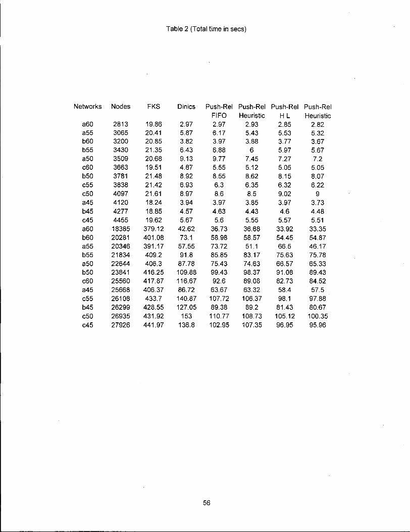
Table 2 (Total time in sees)

Networks Nodes

a60 2813 a55 3065 b60 3200 b55 3430 a50 3509 c60 3663 b50 3781 c55 3838 c50 4097 a45 4120 b45 4277 c45 4455 a60 18385 b60 20281 a55 20346 b55 21834 a50 22644 b50 23841 c60 25560 a45 25668 c55 26108 b45 26299 c50 26935 c45 27926

FKS Dinics

19.86 2.97 20.41 5.87 20.85 3.82 21.35 6.43 20.68 9.13 19.51 4.87 21.48 8.92 21.42 6.93 21.61 8.97 18.24 3.94 18.85 4.57 19.62 5.67

379.12 42.62 401.08 73.1 391.17 57.55 409.2 91.8 406.3 87.78

416.25 109.88 417.87 116.67 406.37 86.72 433.7 140.87

428.55 127.05 431.92 153 441.97 136.8

Push-Rel Push-Rel FIFO Heuristic 2.97 2.93 6.17 5.43 3.97 3.88 6.88 6 9.77 7.45 5.55 5.12 8.55 8.62 6.3 6.35 8.6 8.5 3.97 3.85 4.63 4.43 5.6 5.55

36.73 36.68 58.98 58.57 73.72 51.1 85.85 83.17 75.43 74.63 99.43 98.37 92.6 89.08

63.67 63.32 107.72 106.37 89.38 89.2 110.77 108.73 102.95 107.35

Push-Rel Push-Rel H L Heuristic 2.85 2.82 5.53 5.32 3.77 3.67 5.97 5.67 7.27 7.2 5.05 5.05 8.15 8.07 6.32 6.22 9.02 9 3.97 3.73 4.6 4.48 5.57 5.51 33.92 33.35 54.45 54.87 66.5 46.17 75.63 75.78 66.57 65.33 91.08 89.43 82.73 84.52 58.4 57.5 98.1 97.88 81.43 80.67 105.12 100.35 96.95 95.96

56

Table 3 (FKS)

Network Nodes Solution Total Difference a60 2813 19.78 19.86 0.08 a55 3065 20.33 20.41 0.08 b60 3200 20.73 20.85 0.12 b55 3430 21 21.35 0.35 a50 3509 20.62 20.68 0.06 c60 3663 19.35 19.51 0.16 b50 3781 21.38 21.48 0.1 c55 3838 21.37 21.42 0.05 c50 4097 21.4 21.61 0.21 a45 4120 18.2 18.24 0.04 b45 4277 18.63 18.85 0.22 c45 4455 18.97 19.62 0.65 a60 18385 379.05 379.12 0.07 b60 20281 401.03 401.08 0.05 a55 20346 391.12 391.17 0.05 b55 21834 409.13 409.2 0.07 a50 22644 405.98 406.3 0.32 b50 23841 416.18 416.25 0.07 c60 25560 417.22 417.87 0.65 a45 25668 406.3 406.37 0.07 c55 26108 433.63 433.7 0.07 b45 26299 428.5 428.55 0.05 c50 26935 431.83 431.92 0.09 c45 27926 441.87 441.97 0.1

Time versus Nodes (Sab02)

450 - p s r 5 = = , , , i - ^ —

370 -| , , i i , 1 , , , !| 18000 19000 20000 21000 22000 23000 24000 25000 26000 27000 28000

N o d e s

57

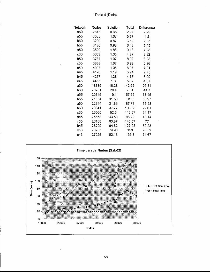
Table 4 (Dinic)

Network Nodes Solution Total Difference a60 2813 0.68 2.97 2.29 a55 3065 1.67 5.87 4.2 b60 3200 0.87 3.82 2.95 b55 3430 0.98 6.43 5.45 a50 3509 1.85 9.13 7.28 c60 3663 1.05 4.87 3.82 b50 3781 1.97 8.92 6.95 c55 3838 1.67 6.93 5.26 c50 4097 1.96 8.97 7.01 a45 4120 1.19 3.94 2.75 b45 4277 1.28 4.57 3.29 c45 4455 1.6 5.67 4.07 a60 18385 16.28 42.62 26.34 b60 20281 28.4 73.1 44.7 a55 20346 19.1 57.55 38.45 b55 21834 31.53 91.8 60.27 a50 22644 31.85 87.78 55.93 b50 23841 37.27 109.88 72.61 c60 25560 52.5 116.67 64.17 a45 25668 43.58 86.72 43.14 c55 26108 63.87 140.87 77 b45 26299 64.82 127.05 62.23 C50 26935 74.98 153 78.02 c45 27926 62.13 136.8 74.67


160

0 -| 1 1 = H 1 1 18000 20000 22000 24000 26000 28000

Nodes

58

Table 5 (Push relabel(FIFO))

Network Nodes Solution Total Difference a60 2813 0.63 2.97 2.34 a55 3065 1.17 6.17 5 b60 3200 0.97 3.97 3 b55 3430 1.87 6.88 5.01 a50 3509 1.65 9.77 8.12 c60 3663 1.33 5.55 4.22 b50 3781 1.9 8.55 6.65 c55 3838 1.32 6.3 4.98 c50 4097 1.8 8.6 6.8 a45 4120 1.13 3.97 2.84 b45 4277 1.23 4.63 3.4 c45 4455 1.47 5.6 4.13 a60 18385 10.65 36.73 26.08 b60 20281 16.62 58.98 42.36 a55 20346 20.73 73.72 52.99 b55 21834 25.9 85.85 59.95 a50 22644 20.73 75.43 54.7 b50 23841 27.5 99.43 71.93 c60 25560 28.47 92.6 64.13 a45 25668 20.88 63.67 42.79 c55 26108 31.18 107.72 76.54 b45 26299 28.32 89.38 61.06 c50 26935 30.43 110.77 80.34 c45 27926 33.06 102.95 69.89


120 -i

18000 20000 22000 24000 26000 28000

Nodes

59

Table6(Heuristic(FIF0))

Network Nodes Solution Total Difference a60 2813 0.55 2.93 2.38 a55 3065 1.03 5.43 4.4 b60 3200 0.77 3.88 3.11 b55 3430 1.32 6 4.68 a50 3509 1.52 7.45 5.93 c60 3663 1.23 5.12 3.89 b50 3781 1.97 8.62 6.65 c55 3838 1.33 6.35 5.02 c50 4097 1.78 8.5 6.72 a45 4120 0.98 3.85 2.87 b45 4277 1.12 4.43 3.31 c45 4455 1.43 5.55 4.12 a60 18385 9.4 36.68 27.28 b60 20281 15.12 58.57 43.45 a55 20346 14.08 51.1 37.02 b55 21834 22.22 83.17 60.95 a50 22644 19.55 74.63 55.08 b50 23841 25.63 98.37 72.74 c60 25560 23.78 89.08 65.3 a45 25668 19.27 63.32 44.05 c55 26108 28.55 106.37 77.82 b45 26299 26.38 89.2 62.82 c50 26935 30.08 108.73 78.65 c45 27926 27.18 107.35 80.17

Time versus Nodes (Sab02) 120 -,

0 -| 1 , , i 1

18000 20000 22000 24000 26000 28000

Nodes

60

Table 7 (Push relabel(HL))

Network Nodes Solution Total Difference a60 2813 0.47 2.85 2.38 a55 3065 0.88 5.53 4.65 b60 3200 0.77 3.77 3 b55 3430 0.85 5.97 5.12 a50 3509 1.23 7.27 6.04 c60 3663 1.12 5.05 3.93 b50 3781 1.45 8.15 6.7 c55 3838 1.18 6.32 5.14 c50 4097 1.41 9.02 7.61 a45 4120 1.03 3.97 2.94 b45 4277 1.37 4.6 3.23 c45 4455 1.2 5.57 4.37 a60 18385 8.27 33.92 25.65 b60 20281 13.21 54.45 41.24 a55 20346 13.43 66.5 53.07 b55 21834 16.07 75.63 59.56 a50 22644 15.75 66.57 50.82 b50 23841 19.32 91.08 71.76 c60 25560 19.9 82.73 62.83 a45 25668 15.95 58.4 42.45 c55 26108 21.93 98.1 76.17 b45 26299 20.97 81.43 60.46 c50 26935 26.89 105.12 78.23 c45 27926 22.95 96.95 74


120

0 -I 1 , 1—1 18000 20000 22000 24000 • 26000 28000

Nodes

61

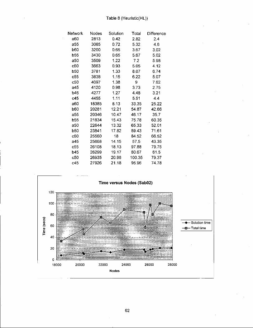
Table 8 (Heuristic(HL))

Network Nodes Solution Total Difference a60 2813 0.42 2.82 2.4 a55 3065 0.72 5.32 4.6 b60 3200 0.65 3.67 3.02 b55 3430 0.65 5.67 5.02 a50 3509 1.22 7.2 5.98 c60 3663 0.93 5.05 4.12 b50 3781 1.33 8.07 6.74 c55 3838 1.15 6.22 5.07 c50 4097 1.38 9 7.62 a45 4120 0.98 3.73 2.75 b45 4277 1.27 4.48 3.21 c45 4455 1.11 5.51 4.4 a60 18385 8.13 33.35 25.22 b60 20281 12.21 54.87 42.66 a55 20346 10.47 46.17 35.7 b55 21834 15.43 75.78 60.35 a50 22644 13.32 65.33 52.01 b50 23841 17.82 89.43 71.61 c60 25560 18 84.52 66.52 a45 25668 14.15 57.5 43.35 c55 26108 18.13 97.88 79.75 b45 26299 19.17 80.67 61.5 c50 26935 20.98 100.35 79.37 c45 27926 21.18 95.96 74.78


120 -

18000 20000 22000 24000 26000 28000

Nodes

62

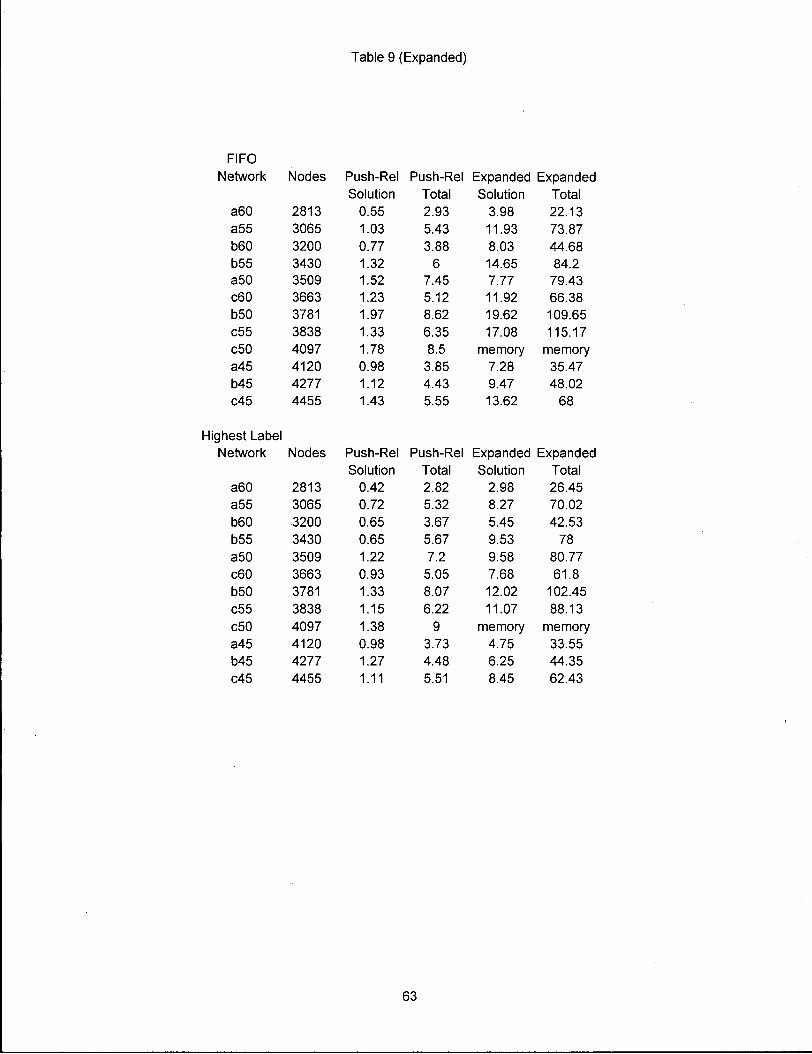
Table 9 (Expanded)

FIFO Network Nodes Push-Rel Push-Rel Expanded Expanded

Solution Total Solution Total a60 2813 0.55 2.93 3.98 22.13 a55 3065 1.03 5.43 11.93 73.87 b60 3200 0.77 3.88 8.03 44.68 b55 3430 1.32 6 14.65 84.2 a50 3509 1.52 7.45 7.77 79.43 c60 3663 1.23 5.12 11.92 66.38 b50 3781 1.97 8.62 19.62 109.65 c55 3838 1.33 6.35 17.08 115.17 c50 4097 1.78 8.5 memory memory a45 4120 0.98 3.85 7.28 35.47 b45 4277 1.12 4.43 9.47 48.02 c45 4455 1.43 5.55 13.62 68

Highest Label Network Nodes Push-Rel Push-Rel Expanded Expanded

Solution Total Solution Total a60 2813 0.42 2.82 2.98 26.45 a55 3065 0.72 5.32 8.27 70.02 b60 3200 0.65 3.67 5.45 42.53 b55 3430 0.65 5.67 9.53 78 a50 3509 1.22 7.2 9.58 80.77 c60 3663 0.93 5.05 7.68 61.8 b50 3781 1.33 8.07 12.02 102.45 c55 3838 1.15 6.22 11.07 88.13 c50 4097 1.38 9 memory memory a45 4120 0.98 3.73 4.75 33.55 b45 4277 1.27 4.48 6.25 44.35 c45 4455 1.11 5.51 8.45 62.43

63

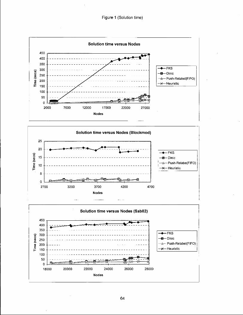
Figure 1 (Solution time)

Solution time versus Nodes

— • — F K S

—{§— Dinic

— * — Push-Relabel(FIFO)

—X—Heuristic

12000 17000

Nodes 22000 27000

25

20

15

I 10

0 4-2700

Solution time versus Nodes (Blockmod)

•FKS

- Dinic

Push-Relabe(FIFO)

-X— Heuristic

3200 3700

Nodes 4200 4700

Solution time versus Nodes (Sab02)

«• 300 | 250 "| 200

150 100 50

0 18000

• • — F K S

•—Din ic

-is— Push-Relabel(FIFO)

Heuristic

20000 22000 24000 26000 28000

Nodes

64

Figure 2 (Solution time no FKS)


•Dinic

-Push-Relabel(FIFO)

-Heuristic


•Dinic

-Push-Relabel(FIFO)

Heuristic

1 8 0 0 0 2 0 0 0 0 2 2 0 0 0 2 4 0 0 0

N o d e s

2 6 0 0 0 2 8 0 0 0

65

Figure 3 (Solution time)

25

20 -k 15

10


- •—Dinic - » - F K S ~ * Series3 - H — Heuristic I

^ ^ S B

2800 3000 3200 3400 3600 3800 4000 4200 4400

Nodes


450

400

350

250 17 300 o

~V 200

H 150

18000 20000 22000 24000

Nodes

26000 28000

- • — F K S - • — Dinic ~ i t — Push-Relabel(HL) | -X—Heuristic

66

Figure 4 (Solution time no FKS)

Solution time versus nodes (Blockmod)

( A O

a E

2800

• Dinic

-Push-Relabel(HL)

•Heuristic

3300 3800

N o d e s

4300


-Dinic

-Push-Relabel(HL)

-Heuristic

18000 20000 22000 24000 26000 28000

N o d e s

67

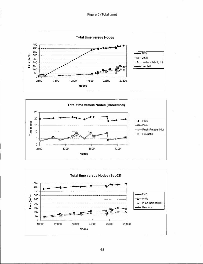
Figure 5 (Total time)

Total time versus Nodes

2800 7800 12800 17800 22800 27800

Nodes

Total time versus Nodes (Blockmod)

25

20 -b-15

1 10

2800 3300 3800 4300

-•—FKS -f§— Dinic

™ir- - Push-Relabel(HL)

- X — Heuristic

Nodes

Total time versus Nodes (Sab02)

-•—FKS - *—Dinic

- A — Push-Relabel(HL) |

-H—Heuristic

18000 20000 22000 24000

Nodes

26000 28000

68

Log(Sol. time) vs Log(No.Nodes)

Dinitz

o (/} at o

•Seriesl

3.4 3.6 3.8 4 4.2

Log Nodes

4.4 4.6

FKS

-Seriesl

3.8 4 4.2

Log Nodes

4.6

Push-Relabel

o in ui o

2.8

2.3

1.8

1.3

0.8

0.3

-0.2

-Seriesl

3.4 3.6 3.8 4 4.2

Log Nodes

4.4 4.6

69

R E F E R E N C E S A N D B I B L I O G R A P H Y

1. Caccetta, L. And L. M . Giannini (1985), On bounding techniques for the open pit limit problem, Proceedings of the Australasian Institute of Mining and Metallurgy 290, 87-89.

2. Caccetta, L. and L. M . Giannini (1986), Optimisation techniques for the open pit limit problem, Proceedings of the Australasian Institute of Mining and Metallurgy 291, 57-63.

3. Caccetta, L. andL. M . Giannini (1988a), An application of discrete mathematics in the design of an open pit limit, Discrete Applied Mathematics 21, 1-19.

4. Caccetta, L. andL. M . Giannini (1988b), The generation of minimum search patterns in the optimum design of open pit mines, Proceedings of the Australasian Institute of Mining and Metallurgy 293, 57-61.

5. Caccetta, L. andL. M . Giannini (1990), Application of Operations Research techniques in open pit mining, Asian-Pacific Operations Research: APORS'88, 707-724

6. Chen, T., 1976," 3D Pit Design with variable wall slope capabilities, "14th Applications of Computers in the mineral Industries Symposium, R. V. Ramani, ed., AIME, New York.

7. Cherkassky, B.V. and Goldberg, A.V. (1994), On implementing Push-Relabel Method for the Maximum Flow problem, Technical Report Stanford University.

8. Faaland, B., Kim. K. and Schmitt. T., 1990, A new algorithm for computing the maximal closure of a graph, Management Science, Vol. 36, No.3.

9. Johnson, T.B., 1973, " A Comparative Study of Methods for determining Ultimate Open-Pit Mining Limits," 11th Applications of Computers in the Mineral Industries Symposium, University of Arizona, Tucson, AZ.

10. Johnson, T.B., 1968, " Optimum Open-Pit Mine Production Scheduling, "Operations Research Centre, University of California, Berkeley, 120 pp.

11. Johnson, T.B., and Sharp, W. R., 1971, A Three-Dimensional Dynamic Programming Method for Optimal Open Pit Design, U S B M Report of Investigations 7553.

12. Kim, Y.C. , 1978. "Ultimate Pit Limit Design Methodologies using Computer Models-The State of the Art," Mining Engineering, October 1978, pp. 1454-1459.

70

13. Kim, Y.C. , Cai, W., and Meyer, W.L., Comparison of microcomputer-based optimum pit limit design algorithms, "Society of Mining Engineers.

15. Lemieux, Marc, 1979, "Moving Cone Optimising Algorithm", Computer Methods for the 80's in the Mineral Industry, ed. A. Weiss, Port City Press, Baltimore, M D , pp. 329-345.

16. Lerchs, H. , Grossmann, IF., 1965, Optimum Design of Open-Pit Mines" Transactions, C.I.M., Vol. LXV111, pp. 17-24.

17. Lipkewich, M.P., Borgman, L., 1969, "Two-and-Three Dimensional Pit Design Optimisation Techniques", A Decade of Digital Computing in the Minerals Industry, ed. A. Weiss, SME of ATME, New York, pp. 505-523.

18. Picard, J., 1976, Maximal Closure of a Graph and applications to combinatorial problems. Management Science, Vol. 22, No. 11.

71

Documents

APPLICATION OF PUSH-RELABEL AND HEURISTICS TO OPEN PIT