Embed Size (px)
Citation preview
Application of Optimization Methods to Controller Design for Active Suspensions
Von der Fakultät für Maschinenbau, Elektrotechnik und Wirtschaftsingenieurwesen
der Brandenburgischen Technischen Universität Cottbus zur Erlangung des
akademischen Grades eines Doktor-Ingenieurs genehmigte Dissertation
vorgelegt von
Tuan-Anh Nguyen, M.Sc.,
geboren am 03.01.1972 in Hanoi, Vietnam
Vorsitzender: Prof. Dr.-Ing. Peter Steinberg
Gutachter: Prof. Dr.-Ing. habil. Dieter Bestle
Gutachter: Prof. Dr.-Ing. Gerhard Lappus
Tag der mündlichen Prüfung: 06.10.2006

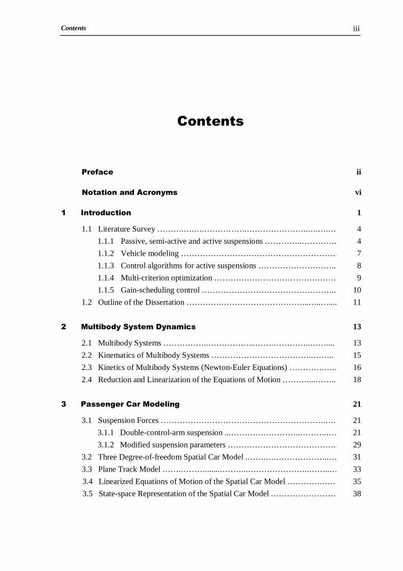
Contents ii
Preface
The work described in this thesis was carried out at the Brandenburg University of
Technology, Cottbus, at the Chair of Engineering Mechanics and Vehicle Dynamics
between April 2003 and October 2006.
First and foremost I would like to express my deepest gratitude to Professor Dieter
Bestle, my research supervisor and reviewer, for whom I have the greatest amount of respect
and admiration. Professor Dieter Bestle not only afforded me the opportunity to study at the
BTU Cottbus, but also provided valuable education and direction in all fields related to this
research. Equally, I am indebted to Professor Gerhard Lappus who did a thorough revision of
the work as second reviewer.
It is a great pleasure to work with the colleagues at the Chair. My special thanks to
Lutz Anklam for supporting the computer facility. I would like to thank Andrej Wachal for
helping me to become familiar with the MATLAB optimization toolbox. I thank Marcin
Beffinger for the valuable discussions on vehicle dynamics. I sincerely thank all the
members of the Chair of Engineering Mechanics and Vehicle Dynamics for creating such a
relaxed and supportive working environment.
This research was funded by the Ministry of Education and Training of Vietnam. I thank
this organization, without whose financial support this work would not have been possible.
Finally, my thanks go to my parents and my wife for the continuous support they
gave while the thesis was taking shape.
Tuan-Anh Nguyen, October 2006.
Preface
Contents iii
Contents
Preface Notation and Acronyms
1 Introduction 1.1 Literature Survey ……….….….…………….…………………..….….…
1.1.1 Passive, semi-active and active suspensions …………..………….
1.1.2 Vehicle modeling …………………………………………………..
1.1.3 Control algorithms for active suspensions ………………………..
1.1.4 Multi-criterion optimization ……………………………………….
1.1.5 Gain-scheduling control …………………………………………...
1.2 Outline of the Dissertation ………….…………………………...…..…....
2 Multibody System Dynamics
2.1 Multibody Systems ……………..……………...…….…………..……....
2.2 Kinematics of Multibody Systems ………………………………..……..
2.3 Kinetics of Multibody Systems (Newton-Euler Equations) ………….…..
2.4 Reduction and Linearization of the Equations of Motion ………....……..
3 Passenger Car Modeling 3.1 Suspension Forces …………………………………………………….….
3.1.1 Double-control-arm suspension ...……………………..………..…
3.1.2 Modified suspension parameters …………………………………..
3.2 Three Degree-of-freedom Spatial Car Model .…….….………………..…
3.3 Plane Track Model …….……….......………..…………………..……..…
3.4 Linearized Equations of Motion of the Spatial Car Model ………….……
3.5 State-space Representation of the Spatial Car Model …………………….
ii
vi
1
4
4
7
8
9
10
11
13
13
15
16
18
21
21
21
29
31
33
35
38

Contents iv
3.5.1 General applied forces …………………………...…………….….
3.5.2 Linear parameter-varying spatial car model …………………...….
3.6 Simulation Model of the Spatial Car ……………………...……….…...…
4 Linear Quadratic Regulator (LQR) Control
4.1 LQR Problem for Linear Systems without Disturbances ……….…….….
4.1.1 Definition of the LQR problem ……….……………….………..…
4.1.2 LQR solution using Pontryagin’s maximum principle ……........…
4.1.3 Algebraic Riccati equation ………..……………….…………..….
4.2 LQR for Linear Systems with Measurable Disturbances …………………
4.2.1 Problem definition …………………………..………..……………
4.2.2 Solution based on Pontryagin’s maximum principle ……….…..…
4.3 Application of LQR Control to the Spatial Car Model …….………...…..
4.3.1 Dynamic criteria for the spatial car model .………….….………...
4.3.2 Spatial car model simulation ………………………….………...…
4.3.3 LQR design for the spatial car model …………………..…………
5 Multi-criterion Optimization (MCO)
5.1 Overview on Multi-criterion Optimization ……………..….………...……
5.2 Multi-criterion Optimization Methods …….…………..………….………
5.2.1 Compromise method ……………..………….………..….………..
5.2.2 Recursive knee approach ……………..…………..………….……
5.3 MCO Problem for Passive Suspension …………....…………..……..…...
5.3.1 Problem definition …………..…………...…………...…….……..
5.3.2 Optimization results based on compromise method ………….…...
5.4 MCO Problem for Active Suspension …….………..…………….............
5.4.1 Problem definition …………..……………….…………..………..
5.4.2 MCO with LQR control ………………….……………...…..…….
5.4.3 Optimization results based on compromise method …………...….
5.4.4 Optimization results based on recursive knee approach ……….….
5.5 MCO Problem for Passive and Active Suspensions …………..……...…...
5.5.1 Problem definition …………..…………...…………...…….……..
5.5.2 Optimization results .………………………………………….…...
38
42
45
46
46
47
48
51
53
53
54
58
58
59
60
64
64
68
68
70
73
73
73
76
76
77
79
82
85
85
86
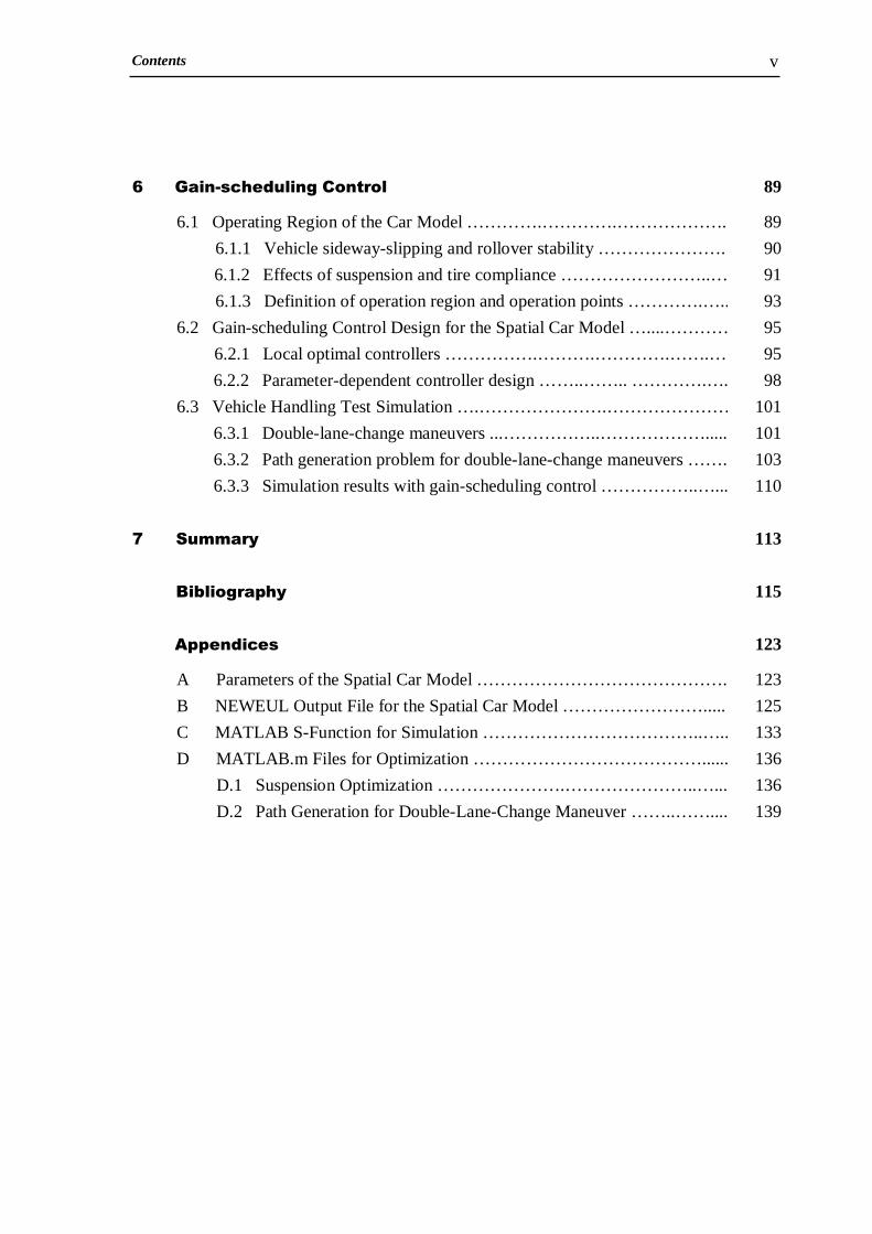
Contents v
6 Gain-scheduling Control 6.1 Operating Region of the Car Model ………….………….………………..
6.1.1 Vehicle sideway-slipping and rollover stability ………………….
6.1.2 Effects of suspension and tire compliance ……………………..…
6.1.3 Definition of operation region and operation points ………….…..
6.2 Gain-scheduling Control Design for the Spatial Car Model …....…………
6.2.1 Local optimal controllers …………….……….………….…….…
6.2.2 Parameter-dependent controller design ……..…….. ………….…..
6.3 Vehicle Handling Test Simulation ….………………….…………………
6.3.1 Double-lane-change maneuvers ...……………..……………….....
6.3.2 Path generation problem for double-lane-change maneuvers …….
6.3.3 Simulation results with gain-scheduling control ……………..…...
7 Summary Bibliography
Appendices A Parameters of the Spatial Car Model …………………………………….
B NEWEUL Output File for the Spatial Car Model …………………….....
C MATLAB S-Function for Simulation ………………………………..…..
D MATLAB.m Files for Optimization …………………………………......
D.1 Suspension Optimization ………………….…………………..…...
D.2 Path Generation for Double-Lane-Change Maneuver ……..……....
89
89
90
91
93
95
95
98
101
101
103
110
113
115
123
123
125
133
136
136
139

Contents vi
Notation and Acronyms Mathematical Symbols
∀
\
■
∃ , ∃/
∈,∉
⊂ ,⊄
∨∧ ,
{ a1, a2,…, an}
{ a | ... }
A ∩B
A ∪B
A \ B
nI
RI
nRI mn x RI
| a |
a := b,
a = b
a ≥ b, a ≤ b
a << b
a ≈ b
i = j (k) n
diag{ a1, a2,…, an}
max{a1, a2,…, an}
min{a1, a2,…, an}
for all
not including, except
end of proof
there exists, exists not
element of, not element of
subset of, not subset of
logical and, or
set of elements a1, a2,…, an
set of all a satisfying conditions …
intersection set of A and B : { }B AB A a a |a ∈∧∈=∩
union set of A and B : { }B AB A a a |a ∈∨∈=∪
A without B : { }B AB A a a |a ∉∈= ,\
set of n integers {1, 2,…, n}
set of real numbers
set of n-dimensional real vectors
set of n x m matrices with elements fromRI
absolute value of a
a defined as b
a has to be identical to b
a is larger or equal, smaller or equal to b
a is much smaller than b
a is approximately b
i runs from j to n with steps k
n x n diagonal matrix with a1, a2,…, an on its diagonal
maximum value among a set of elements a1, a2,…, an
minimum value among a set of elements a1, a2,…, an
!
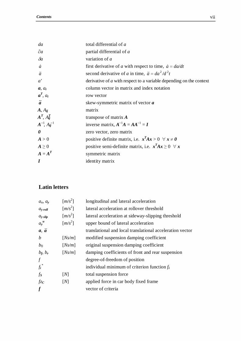
Contents vii
da
∂a
δa
a&
a&&
a’
a, ai
aT, ai
a~
ijA A , Tij
TA A , 11, −−
ijA A
0
A > 0
A ≥ 0
A = AT
I
total differential of a
partial differential of a
variation of a
first derivative of a with respect to time, da/dta =&
second derivative of a in time, t/ddaa 22=&&
derivative of a with respect to a variable depending on the context
column vector in matrix and index notation
row vector
skew-symmetric matrix of vector a
matrix
transpose of matrix A
inverse matrix, A−1A = AA−1 = I
zero vector, zero matrix
positive definite matrix, i.e. xTAx > 0 ∀ x ≠ 0
positive semi-definite matrix, i.e. xTAx ≥ 0 ∀ x
symmetric matrix
identity matrix Latin letters
ax, ay
ay roll
ay slip
ayu
a, a
b
b0
bf, br
f
fi *
fS
fzC
f
[m/s2]
[m/s2]
[m/s2]
[m/s2]
[Ns/m]
[Ns/m]
[Ns/m]
[N]
[N]
longitudinal and lateral acceleration
lateral acceleration at rollover threshold
lateral acceleration at sideway-slipping threshold
upper bound of lateral acceleration
translational and local translational acceleration vector
modified suspension damping coefficient
original suspension damping coefficient
damping coefficients of front and rear suspension
degree-of-freedom of position
individual minimum of criterion function fi
total suspension force
applied force in car body fixed frame
vector of criteria

Contents viii
ra ff ,
fA, fB, fK
fS
g
g
g
h
hC
hR
hRC
hRV
h
h
k
k0
kf, kr
kx
kw
l
lf, lr
lβ, lα k
ra ll ,
m
mi
mS
mU
n
n
n
p
p0
p*
p EP
pl, pu
[m/s2]
[m]
[m]
[m]
[m]
[N/m]
[N/m]
[N/m]
[m]
[Nm]
[Nm]
[kg]
[kg]
[kg]
vector of applied and reaction forces
vector of anti-roll, damper and spring forces
vector of total suspension forces
gravity acceleration (9.81 m/s2)
vector of generalized constraint forces
vector of equality constraints
number of design variables
static height of the car’s center of gravity above ground
height of suspension roll center above ground
distance from roll axis to the car’s center of gravity
distance from ground to roll axis
vector of excitation forces
vector of inequality constraints
translational stiffness
original suspension stiffness
stiffness of front and rear suspension
component of state-feedback gain matrix
component of disturbance-feed forward gain matrix
number of equality constraints
distance from the car’s center of gravity to front and rear axles
applied roll and pitch moment in the car body fixed frame
vector of Coriolis and centrifugal forces
vector of applied, reaction moments
number of constant curvatures of vehicle path model
mass of body i
sprung mass
unsprung mass
number of criteria
number of points changing curvature of vehicle path model
normal vector of convex hull of the individual minima
number of rigid bodies
initial point design
optimal design
Edgeworth-Pareto optimal design
vector of lower and upper variable bounds
Contents ix
q
q
qa aq , cq
r
r0
rf, rr
rk
r
s
t
tk
tw
twf, twr
u
u0
u
ux, uw
v
v, v wi
w
x, y, z
xwi, ywi
x
y
y
zC
zS
zSi
zU
z
zS
A, B, Bw
BS
[N/m/rad]
[Nm/rad]
[N/m/rad]
[m]
[m]
[s]
[s]
[m]
[m]
[N]
[N]
[N]
[N]
[m/s]
[m]
[m]
[m]
[m]
[m]
number of independent constraints
vector of generalized applied forces in inertial coordinate system
vector of generalized applied forces in the car body fixed frame
global vector of applied forces, Coriolis and centrifugal forces
modified rotational stiffness of anti-roll bar
original anti-roll bar rotational stiffness
rotational stiffness of front and rear anti-roll bar
rate of curvature change
position vector
track coordinate
time
time point of changing curvature
mean value of half-track width
half track width of front and rear axle
control force
original control force
vector of controlled forces
state-feedback and disturbance feed-forward control
longitudinal velocity
translational and local translational velocity
weighting factor of criterion i
vector of exogenous disturbances
axes of reference frame
longitudinal and lateral position of the ith wheel in car body system
state vector
vector of generalized coordinates
vector of measured outputs
vertical displacement of the car’s center of gravity
vertical displacement of sprung mass
vertical displacement of the ith suspension node
vertical displacement of unsprung mass
vector of generalized velocities
vector of vertical displacement of suspension nodes
state matrices
suspension damping matrix

Contents x
C, D, Dw
D
F
F EP
Fz-in, Fz-out
Fy-in, Fy-out
FA, FB, FK
FC
FU
F
G
��
IX, IY, IZ
Ii
J
JT, JR
J
K
K, Kx
Kw
KA
KS
L
MU
M , M
N
P
P EP
P
P
Q
Q, Qy
Q
R
Rmin
[N]
[N]
[N]
[N]
[N]
[kg m2]
[Nm]
[m]
[m]
measurement matrices
matrix of damping forces
feasible criterion space
Edgeworth-Pareto optimal set in design space
total normal load on inside and outside wheels
total lateral force on inside and outside wheels
anti-roll, damper and spring force
control force
anti-roll force acting on unsprung mass
translational distribution matrix
matrix of gyroscopic forces
Hamiltonian function
roll, pitch and yaw moment of inertia of car body
inertia tensor of body i
objective function
translational and rotational Jacobi matrix
global Jacobi matrix
stiffness matrix
gain matrix of state-feedback controller
gain matrix of disturbance-feed forward controller
anti-roll stiffness matrix
suspension stiffness matrix
rotational distribution matrix
anti-roll moment
mass matrix, global mass matrix
matrix of non-conservative forces
feasible design space
Pareto frontier or trade-off curve of non-dominated solutions
matrix of velocity-dependent forces
Riccati matrix
matrix of position-dependent forces
weighting matrix of states and measured outputs
global distribution matrix of reaction forces
track curve radius
minimum turning radius

Contents xi
R, Ru
S T Xwi, Ywi
XV, YV
lwY , u
wY l
coneY , uconeY
[s]
[m]
[m]
[m]
[m]
weighting matrix of controlled forces
rotation matrix
simulation time
longitudinal and lateral position of the ith wheel in inertial system
longitudinal and lateral position of car in inertial coordinate system
lower and upper bound on wheel tracks
lateral position of lower and upper cones Greek letters
α
iα , iα
β
β&&
γ uγ&
δ
δW
εi
θ
κ
κj
λ
λ
ξ
ξ0
ξ φ0, φC 0
µy
iω , iω
∆l
∆z
[rad]
[rad]
[rad/s2]
[rad]
[rad/s]
[m]
[J]
[rad]
[m–1]
[m–1]
[rad]
[rad]
[rad]
[m]
[m]
car body pitch angle
angular and local angular acceleration vector of body i
car body roll angle
car body roll acceleration
yaw angle
uper bound on yaw rate
displacement of suspension connecting points
virtual work
constraint on criterion fi for compromise method
slope angle of car body roll axis
track curvature
constant path curvature
modified coefficient of suspension parameters
dynamic Lagrange multipliers
angular displacement of unsprung mass
directional angle of lower control arm
Riccati vector
directional angle of spring-damper and actuator
road friction coefficient
angular and local angular velocity vector of body i
dynamic deflection of spring-damper
relative vertical displacement of sprung and unsprung mass

Contents xii
List of Acronyms
ARE
CG
CHIM
CUSC
DRE
DAE
DLC
DoF
EP
ISO
LQR
LPV
LTI
LTV
MBS
MCO
NBI
ODE
RMS/r.m.s
Algebraic Riccati Equation
Center of Gravity
Convex Hull of Individual Minima
Consumers Union Short Course
Differential Riccati Equation
Differential-Algebraic Equations
Double-Lane-Change
Degree-of-Freedom
Edgeworth-Pareto
International Organization for Standardization
Linear Quadratic Regulator
Linear Parameter-Varying
Linear Time-Invariant
Linear Time-Varying
Multi-Body System
Multi-Criterion Optimization
Normal-Boundary Intersection
Ordinary Differential Equations
Root Mean Square

Chapter 1 - Introduction 1
Chapter 1
Introduction
Demands for better ride comfort, road handling and controllability of passenger cars have
motivated automotive industries to consider the use of active and semi-active suspensions.
Many analytical and experimental studies on active and semi-active suspensions to
improve ride quality and handling performance have been performed. The conclusion is
that active and semi-active suspensions can provide substantial performance
improvements over passive suspensions in general.
The effectiveness of the active suspension system on vehicle dynamics is analyzed
based on vehicle models. Passenger cars are complex multibody systems consisting of
many rigid and deformable components, Popp and Schiehlen [59], Rahnejat [60], Rill [63]
and Willumeit [92]. A full vehicle model needs to present the nonlinear kinematics of wheels
and axles, the effects of suspension geometry and has to include the drive train, the steering
mechanism and the tire dynamics, Kortüm and Lugner [42], resulting in a high number of
degrees of freedom. Since it makes no sense to try to build a universal vehicle model that
can be used to solve all dynamic problems, reduced dynamic models for specific
investigation purposes are often designed instead, Eberhard and Schiehlen [24] and Rettig
and Stryk [62]. The vehicle yaw dynamics is mainly studied based on the conventional
planar models such as single track model, Ammon [2], Mitschke [51] and Wallentowitz [87],
or double track model, Ackermann [1], Halfmann and Holzmann [36] and Kiencke and
Nielsen [40], where the effects of active suspensions are not taken into consideration. On
the other hand, yaw motion is usually neglected when the quarter-car, half-car or spatial-car
model with active or semi-active suspensions are investigated. In order to study the effects
of active suspensions on the vehicle yaw dynamics, a proper mathematical model of the
vehicle must be established that can describe the dynamic characteristics of interest
sufficiently, but at the same time can be easily treated in control synthesis.

Chapter 1 - Introduction 2
The application of active suspensions involves indispensably the application of
control algorithms. Active control concepts have been investigated extensively over the
past ten years. The purpose of an optimal control problem is to determine the control
policy optimizing specific criteria, subject to the constraints imposed by the physical
nature of the problem. One of the most effective optimal control techniques commonly
used in engineering is the linear quadratic regulator (LQR) control, Colaneri, et al. [14],
Ramirez [61], Schwarz [71] and Siouris [75]. For linear systems whose states can be
measured online, the LQR algorithm results in a simple state-feedback control structure
and provides an easy way to derive the optimal controller. By choosing appropriately the
weighting factors corresponding to the criteria of interest, the optimal controller can be
immediately obtained via MATLAB software. However, the standard LQR problem is
defined only for linear systems without disturbances. In practice, dynamic systems usually
are affected by exogenous excitations. Therefore, a control law with state-feedback and
disturbance-feed forward controllers has been applied by several investigators as an
optimal solution for the disturbance-rejection control problem, e.g. Ackermann [1], Bail [4]
and Sampson [67]. Different formulas for the controllers have been applied without
theoretical basis. Therefore, developing the LQR problem for excited linear-systems to
affirm the control law as well as to define correctly the optimal controllers is necessary.
Another approach to achieve the optimal controller is multi-criterion optimization
(MCO). Once the control structure is determined, the optimal components of the controller
can be obtained from the associated multi-criterion optimization problem. Furthermore, the
best trade-off between conflicting criteria can be also derived. In order to find the optimal
compromise solutions, which are known as the Edgeworth-Pareto (EP) optimal solutions,
the multi-criterion optimization problem usually has to be reduced to scalar utility
problems, Bestle [7], Das [18] and Eberhard, et al. [22]. Being one of the effective
scalarization approaches, the compromise method can generate an even distribution of the
EP-optimal solutions on the trade-off surface even if the criterion space is non-convex,
Collette and Siarry [16] and Deb [20]. This method, however, results in wasted
computational resources to problems with more than two criteria. To deal with such
problems, the recursive knee approach introduced by Das and Denis [19] and Wachal and
Bestle [86], an advanced optimization method that can create a representative set of the EP-
optimal solutions with a minimal computation effort, should be applied.

Chapter 1 - Introduction 3
Solving the multi-criteria optimization problem directly for the optimal controller
would be time-consuming, especially for large systems where the number of controller
components often is cumbersome. This problem can be solved by the combination of the
LQR algorithm, i.e., instead of finding directly the components of the controllers, the task
of optimization routine is to define the optimal weighting factors of the associated LQR
problem. For each time simulation, the controller results from the LQR algorithm based
on the weighting factors provided by optimization algorithm. By combining multi-
criterion optimization with the LQR control, not only computational time can be reduced
significantly, but also the limitation of the LQR algorithm to the constrained control
problems can be overcome.
A constant optimal controller obtained from the LQR-based optimization method
proposed above, however, is valid only to a specific operation point defined by specific
values of the system parameters. Vehicle dynamic systems usually include parameters
that can be changed arbitrarily by different drive maneuvers or road conditions, thus
resulting in parameter-varying systems. To maintain the desired performances of a
parameter-varying system, the controller has to be able to change its parameters
corresponding to the change of the system varying parameters over their operation
regions, Sastry and Bodson [68]. The process for designing such controllers for
parameter-varying systems is referred to as gain-scheduling control design. Recently,
various gain-scheduling design techniques have been introduced. These methods, however,
require either a complicated control structure, see e.g. Balas, et al. [5] and Genc [32], or a
complex computation procedure, see e.g. Ackermann [1]. Therefore, a strategy for
designing gain scheduling based on the defined optimal control structure and the proposed
optimization method must be studied.
The effectiveness of the designed gain-scheduling controller must be evaluated
through vehicle handling test maneuvers. It is well-known that there are an infinite number
of paths that could satisfy the requirements for the double-lane-change maneuver at a given
speed, which is designated as the standard vehicle handling test. In order to find an optimal
path with respect to specific requirements, the path generation problem must be formulated.
There are several different objectives for path optimization such as optimization of driving
time, deviation from the lane center and driving safety, O’Hara [54]. Aiming to define an
optimal path that enhances driving safety, the vehicle lateral dynamics can be reduced by
minimizing track curvature, and thus minimizing lateral acceleration during the test.
Chapter 1 - Introduction 4
1.1 Literature Survey The description given above shows that, active suspension design relies on the fields of
vehicle dynamic modeling, optimal control, multi-criterion optimization, and gain-
scheduling control. The following sections briefly describe papers relevant and
complementary to this research.
1.1.1 Passive, semi-active and active suspensions The purpose of an automobile suspension is to adequately support the chassis, to maintain
tire contact with the ground, and to manage the compromise between vehicle road handling
and passenger comfort. Depending on the configurations and implementations, vehicle
suspension systems can be classified as passive suspension, semi-active suspension or
active suspension.
When designing a passive suspension, the trade-off mentioned above is made
upfront and cannot be easily changed. For example, a sports car suspension will have
stiffer shock absorbers for better road handling while the shock absorbers on a family
vehicle will be softer for a comfortable ride. In the case of semi-active and active
suspension systems, the trade-off decisions can be changed in real-time.
A semi-active suspension has the ability to change the damping characteristics of
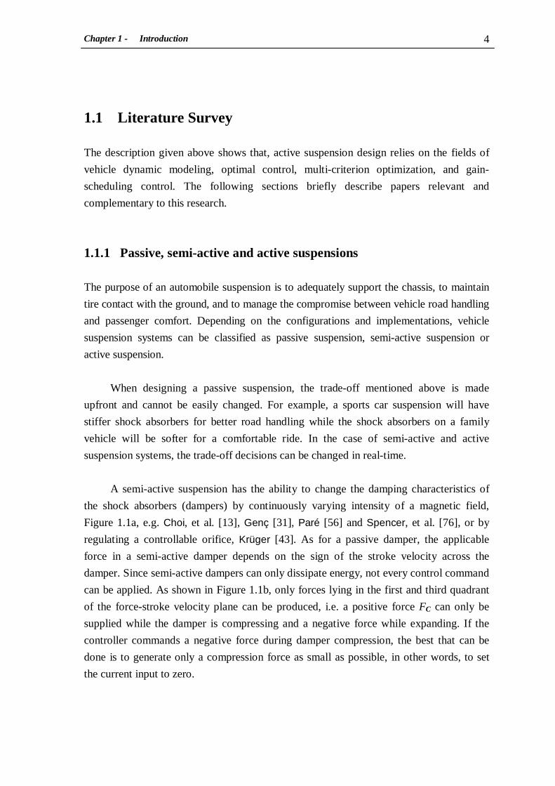
the shock absorbers (dampers) by continuously varying intensity of a magnetic field,
Figure 1.1a, e.g. Choi, et al. [13], Genç [31], Paré [56] and Spencer, et al. [76], or by
regulating a controllable orifice, Krüger [43]. As for a passive damper, the applicable
force in a semi-active damper depends on the sign of the stroke velocity across the
damper. Since semi-active dampers can only dissipate energy, not every control command
can be applied. As shown in Figure 1.1b, only forces lying in the first and third quadrant
of the force-stroke velocity plane can be produced, i.e. a positive force FC can only be
supplied while the damper is compressing and a negative force while expanding. If the
controller commands a negative force during damper compression, the best that can be
done is to generate only a compression force as small as possible, in other words, to set
the current input to zero.

Chapter 1 - Introduction 5
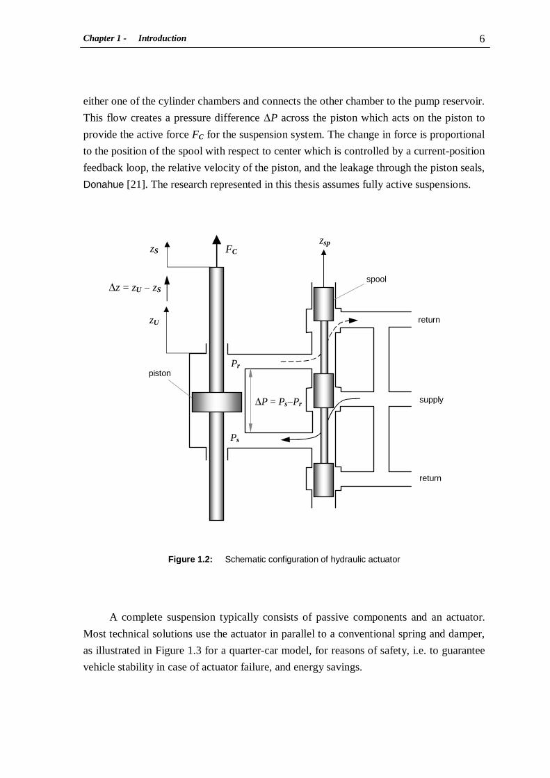
Contrary to semi-active suspensions, hydraulic actuators of fully active suspensions
can generate continuously controlled forces, i.e. they can both add and dissipate energy
from the system, and thus provide better performance than semi-active suspensions. The
hydraulic actuators are typically governed by electro hydraulic servo-valves and are
mounted in parallel to passive suspension springs and dampers, allowing for the
generation of forces between the sprung and unsprung masses. The electro hydraulic
system consists of an actuator, a primary power spool valve and a secondary bypass
valve. As seen in Figure 1.2, the hydraulic actuator cylinder lies in a follower
configuration to a critically centered electro hydraulic power spool valve with matched
and symmetric orifices. Positioning of the spool zsp directs high pressure fluid flow to
Figure 1.1: Schematic configuration (a) and characteristics (b)
of magnetorheological (MR) dampers for different currents
(a)
∆z [cm]
(b)
FC [N]
∆z [cm/s] .
FC [N]
0.00 A 0.25 A 0.50 A 0.75 A
coil
gas chamber
diaphragm
current source
outer cylinder
inner cylinder
MR fluid
MR fluid flow
magnetic field
A
A
magnetic circuit
FC
zS
zU ∆z = zU − zS
Chapter 1 - Introduction 6
either one of the cylinder chambers and connects the other chamber to the pump reservoir.
This flow creates a pressure difference ∆P across the piston which acts on the piston to
provide the active force FC for the suspension system. The change in force is proportional
to the position of the spool with respect to center which is controlled by a current-position
feedback loop, the relative velocity of the piston, and the leakage through the piston seals,
Donahue [21]. The research represented in this thesis assumes fully active suspensions.
A complete suspension typically consists of passive components and an actuator.
Most technical solutions use the actuator in parallel to a conventional spring and damper,
as illustrated in Figure 1.3 for a quarter-car model, for reasons of safety, i.e. to guarantee
vehicle stability in case of actuator failure, and energy savings.
Figure 1.2: Schematic configuration of hydraulic actuator
FC
zsp
spool
piston
Pr
Ps
zS
zU
∆z = zU − zS
∆P = Ps−Pr
return
supply
return

Chapter 1 - Introduction 7
1.1.2 Vehicle modelling Physical models for investigating the vertical dynamics of suspension systems are most
commonly built on the conventional quarter-car model, which represents the vertical
motion of a system including a quarter of the car body and the corresponding wheel, e.g.
Chantranuwathana and Peng [10], Donahue [21], Pang, et al. [55], Shen and Peng [73]
and Yi and Song [94]. To take into account the suspension geometry, Hong, et al. [38]
introduced a plane quarter-car model with a semi-active Mac-Pherson suspension. More
accurate analysis is achieved by extensions to a so-called full-car model, e.g. Choi, et al. [13]
and Park and Kim [57], which reflects both vertical deflections and inclinations. Bounce,
roll and pitch motions of the car body can be investigated simultaneously. In addition, the
effects of suspension geometry and stabilizers or anti-roll bars also can be involved in the
model, e.g. Gärtner and Saeger [30] and Mitschke [50, 51]. Separated and decoupled
investigations are possible using half-car models, e.g. Gaspar, et al. [29], Taghirad and
Esmailzadeh [78] and Vaughan [83].
The most commonly used models for studying vehicle lateral dynamics are the
conventional planar models such as single track model, e.g. Ammon [2], Lazic [45], Lu, et al. [46]
Figure 1. 3: Quarter-car model with active suspension
mU
k b FC
unsprung mass
actuator
mS
sprung mass

Chapter 1 - Introduction 8
and Ryu [65], and double track model, e.g. Ackermann [1], Halfmann and Holzmann [36] and
Kiencke and Nielsen [40]. Although the yaw motion is taken into account, the suspension
effects are not considered for these models. Hyvärinen [39], Sampson and Cebon [66]
and Sampson [67] investigated the effects of the suspension system on vehicle lateral
dynamics based on a half-car roll model. Additionally, the influences of the suspension
and tire deformations on the vehicle stability and handling were also evaluated by Bodie
and Hac [8] and Hac [34, 35].
1.1.3 Control algorithms for active suspensions One of the most straightforward and effective control approaches for active suspensions is
the so-called sky-hook control, which is used to hang up the vehicle body on a virtual sky
completely uncoupled from road excitations. A large number of applications in the literature
exist which often consist the skyhook approach as the reference control law; many of
those investigations have used the quarter car model as a basis, e.g. Choi, et al. [13],
Donahue [21] and Krüger [43]. Analogously, the ground-hook control concept takes into
account wheel oscillations, e.g. Valasek, et al. [82].
Linear quadratic regulator (LQR) is a powerful concept of optimally controlling
linear systems commonly used for vehicle system control. This technique results in a
simple control structure with an optimal state-feedback controller which can easily be
obtained from the solution of the algebraic Riccati equation. Several applications of the
LQR control have been used in active suspension control, e.g. Rettig and Stryk [62],
Sampson [67] and Taghirad and Esmailzadeh [78].
For complex systems where not all states are accessible to be measured, Kalman filter
techniques are often used, Moscinski and Ogonowski [52] and Shahian and Hassul [72].
The LQR control with Kalman filter has been applied in the investigations of Krüger [43],
Venhovens and Nabb [84] and Yi and Song [94]. Another approach proposed by Vaughan [83]
is to use the LQR control with output-feedback controller.
Dealing with the uncertainties in system parameters, many robust control techniques
have been developed. The most commonly used is the H∞ control, e.g. Choi, et al. [13],
Gaspar, et al. [29] and Wu [93]. Additionally, adaptive extensions to the standard LQR
Chapter 1 - Introduction 9
control have been performed, Chantranuwathana and Peng [10]. Beside that, there also
exists a variety of alternative formulations of the problem to control active suspension
systems such as fuzzy logic control, e.g. Krüger [43] and Rouieh and Titli [64], and sliding
mode control, e.g. Chen and Huang [11], Yokoyama, et al. [95] and Zhong [96].
1.1.4 Multi-criterion optimization As already mentioned, suspension design has to resolve the conflict between ride safety and
ride comfort resulting in a multi-criterion optimization problem. There exist a large number
of methods and algorithms for solving such multi-criterion optimization problems, see for
example Andersson [3], Coleman, et al. [15], Collette and Siarry [16], Deb [20] and
Marler and Arora [47]. Most methods attempt to scalarize multiple objectives and perform
repeated applications to find a set of Edgworth Pareto (EP)-optimal solutions, Bestle [7]
and Shukla and Deb [74].
Aiming to provide a good diversity among solutions in the criterion space, beside
the compromise method various advanced algorithms have been developed. The first one
is the normal boundary intersection (NBI) method, developed by Das [17, 18] and Das
and Dennis [19]. Their study was aimed at getting a good diversity of solutions on the
efficient frontier by starting from normal directions to the ideal plane passing through
individual function minimizers. The study used an equality constraint formulation of the
sub-problems. A modified version of the NBI approach, called the recursive knee
approach, was developed by Das and Dennis [19]. Better formulations were also
introduced and programmed by Wachal and Bestle [86].
Kim and Weck [41] developed the adaptive weighted-sum method for multi-criterion
optimization. Initially, the efficient frontier is approximated by employing a single-
objective optimization algorithm with the weighted-sum approach many times. Efficient
front patches are then identified and further refined by using additional equality constraints.
Mattson, et al. [48] and Messac, et al. [49] developed the normal constraint method
for getting an even distribution of the EP-optimal solutions on the Pareto frontier. In the
normal constraint method, there is a sequential reduction of the feasible space by hyper-
planes passing through a point on the ideal plane. Chen, et al. [12] also developed the

Chapter 1 - Introduction 10
physical programming method and then presented a different method for generating the
entire efficient frontier using the physical programming approach.
Over the past decade, the evolutionary multi-objective optimization received growing
attention by its ability for finding multiple EP-optimal solutions in a single simulation run
and providing the entire range of solutions and the shape of the Pareto frontier, Deb [20]
and Shukla and Deb [74]. Applications of the evolutionary multi-objective optimization to
the design of rail vehicle suspensions performed by Eberhard, et al. [23] and He [37]
demonstrated the effectiveness of this method.
1.1.4 Gain-scheduling control Due to arbitrary changes of the system parameters resulting from different drive
maneuvers or road conditions, vehicle dynamic systems are often formulated as
parameter-varying systems which require the controller to change its parameters
appropriately. Gain-scheduling is one of the most intuitive approaches to adaptive control,
commonly used to control linear parameter-varying (LPV) systems. This technique amounts
to design controllers which are able to update their parameters on-line according to the
variations of the system parameters. The advantage of gain-scheduling is that the required
performances of the system are guaranteed by the rapid change of the control parameters in
response to the changes in the system dynamics, Sastry and Bodson [68].
Conventionally, gain-scheduling control is designed by a two-step procedure: first
one designs local controllers at specified operation points, then a parameter-dependent
controller for linear parameter-varying system is scheduled either via a switching scheme,
e.g. Giua, et al. [33], or by interpolating among the local point designs, e.g. Kumar [44].
Robust control techniques such as H2 or H∞ control have recently become a popular
concept in control of linear parameter-varying systems with un-modeled dynamics or
unknown disturbances, e.g. Bruzelius [9], Fujiwara and Adachi [27], Gaspar, et al. [29],
Wang and Tomizuka [89, 90] and Wu [93]. These techniques involve the solution of linear
matrix inequalities and result in a constant state-feedback matrix ensuring that the transfer
function from excitations to controlled outputs is lower than a prescribed small value,
Gahinet, et al. [28]. The set of admissible parameter values can be treated in a direct

Chapter 1 - Introduction 11
manner. In addition, bounds on the rates of change of the parameters can be incorporated
to obtain a less conservative controller, e.g. Wang and Tomizuka [88]. The resulting
controller has a stability and performance guarantee in the pre-defined operation region.
However, a potential problem with these methods is the lack of performance.
Another approach for designing gain-scheduling control is the so-called simultaneous
Γ-stabilization method presented by Ackermann [1] and Wang, et al. [91]. This technique
permits the designer to specify a set of desired regions, joint or disjoint, in the complex root
plane. Then a numerical algorithm is used to find the control parameters such that all the
roots of the closed-loop systems resulting from the linearized plant models are within the
specified regions. Although the performances of the closed-loop system can be improved by
changing the desired regions in the complex plane, the simultaneous Γ-stabilization method
is only suitable to controllers with a few components.
Petersen, et al. [58] use the constrained LQR method to design gain-scheduling for
a wheel-slip-control model, resulting in a parameter-dependent controller scheduled by
the car velocity. Good performance and robustness of the model are shown through
analysis and experimental results. However, this approach is limited within a specific
operation region and requires special experiences for designing the weighting matrices.
1.2 Outline of the Dissertation
Following this introduction chapter, the remainder of the thesis is divided into six
chapters. Chapter 2 describes the fundamentals of multibody system dynamics. The
equations of motion of multibody systems are established based on analyzing the
kinematics and kinetics. Additionally, reduced and linearized forms of the equations of
motion are presented which will be used for control analysis.
In Chapter 3 a three-degree-of-freedom spatial car model for studying the vehicle’s
lateral dynamics is introduced. To define the equations of motion, a plane track model
describing yaw motion of the car is presented. The linearized equations of motion and
their state-space representation are then introduced. Discussions on special cases of the

Chapter 1 - Introduction 12
general spatial car model result in a simplified model to be used for optimal control
analysis. For simulation, a spatial car model is built in MATLAB/Simulink.
An optimal control law for the spatial car model is defined in Chapter 4 based on the
linear quadratic regulator (LQR) control. The LQR problem is shown first for linear
systems without disturbances, which results in an optimal state-feedback controller, and
then extended to linear systems with measurable disturbances, which leads to an optimal
disturbance-feed forward controller. Automotive performance criteria specified for the
spatial car model are also introduced in this chapter. The effectiveness of active
suspensions with LQR control compared to passive suspensions is shown based on
simulation results for the spatial car model.
Some background information on multi-criterion optimization (MCO) is first
presented in Chapter 5. Then, formulations of the compromise method and recursive knee
approach are given in more detail. MCO problems for both passive and active suspension
cases are defined. In order to reduce the number of design variables for the case of active
suspension, an optimization procedure combining the MCO method with the LQR
algorithm is proposed. The advantages as well as drawbacks of the compromise method
compared to the recursive knee approach for finding the Pareto frontier are discussed
based on optimization results.
Chapter 6 introduces the method of designing gain-scheduling control for the linear
parameter-varying spatial car model. First the operation region of the model is determined,
considering the effects of the deformation of suspension and tires on the vehicle stability in
cornering situations. Then, based on the local optimal controllers defined for specified
operation points, a parameter-dependent controller is formulated that is able to vary
continuously its parameters according to the changes of the system’s varying parameters.
To demonstrate the effectiveness of the designed parameter-dependent controller, vehicle
handling test simulations are performed with input parameters obtained from the path
generation problem defined for double-lane-change maneuvers.
Finally, conclusions and recommendations on future research are summarized in
Chapter 7. Appendices provide the parameters of the studied car, the NEWEUL output
file for the spatial car model and MATLAB.m-files used for the various investigations in
this dissertation.

Chapter 2 - Multibody System Dynamics 13
Chapter 2
Multibody System Dynamics
Many mechanical and structural systems such as vehicles, robots, mechanisms, and aircrafts
consist of interconnected components that undergo large translational and rotational
displacements and can be modeled as multibody systems. In this chapter, the kinematics and
kinetics of multibody systems are formulated. Subsequently, the equations of motion of
multibody systems in both nonlinear and linearized form are presented.
2.1 Multibody Systems
In general, a multibody system is defined to be a finite set of elements such as rigid bodies
and/or particles, bearings, joints and supports, springs and dampers, active force and/or
position actuators as illustrated in Figure 2.1 and Figure 2.2. For the mathematical
description of these elements, the following assumptions are agreed upon, Schiehlen [70]:
1. A multibody system consists of rigid bodies and ideal joints. A body may degenerate
to a particle or to a body without inertia. The ideal joints include the rigid joint, the
joint with completely prescribed motion (rheonomic constraint) and the vanishing joint
(free motion).
2. The topology of the multibody system is arbitrary; chains, trees and closed loops are
admitted.
3. Joints and actuators are summarized in open libraries of standard elements.
4. Subsystems may be added to existing components of the multibody system.

Chapter 2 - Multibody System Dynamics 14
Figure 2.2: Elements of multibody systems (and idealizations)
Figure 2.1: Multibody system
rigid body
coupling elements
constraints
yI xI
zI ri
zi yi
xi
Ci
O
rigid body
ideal constraints (rigid, no friction, no mass)
mass elements (no elastic deformation)
bearings, joints
servo motor (position control)
coupling elements (no mass)
mass point
spring
damper
actuator (force control)

Chapter 2 - Multibody System Dynamics 15
The topological structure of a multibody system can be possibly tree structure or
system with closed kinematical loops. The most commonly mentioned classification of
constraints is scleronomic vs. rheonomic according to their time variation characteristic or
holonomic vs. non-holonomic according to the constraint motion type. More detailed
descriptions about multibody systems can be found in Bestle [7], Popp and Schiehlen [59]
and Schiehlen [69].
For dynamical analysis, the multibody system has to be described mathematically by
equations of motions. In the following sections the general theory for holonomic and non-
holonomic systems will be presented using a minimal number of generalized coordinates
for a unique representation of the motion.
2.2 Kinematics of Multibody Systems
There are basically two approaches in choosing coordinates to describe the kinematics of
multibody systems, generalized, i.e. independent, coordinates and dependent coordinates.
The former one leads to a kinematics description in minimal form, whereas the later one
results in the descriptor form. Multibody systems with chain or tree structure can always
be described with generalized coordinates and subsequently by ordinary differential
equations (ODEs). Multibody systems with closed loops on the contrary cannot be always
described with independent coordinates. The introduction of additional dependent
coordinates in this case requires additional algebraic constraint equations resulting in a
coupled differential-algebraic system of equations of motion (DAE).
The degrees of freedom (DoFs) f of a spatial multibody system with p bodies and q
independent constraints can be calculated as f = 6p – q. Accordingly f generalized
coordinates y = [ y1, y2, …, yf ]T can be chosen to describe the translational and rotational
motion of each body Ki, i = 1(1) p. The translation can be described with the position
vector ri of the center of gravity (CG), whereas the orientation may be described by a
matrix of directional cosines Si. In an inertial reference frame, they can be described as
functions of the generalized coordinates of following form:
( )( ) ( )2.1.1(1),,
,,
p i t
t
==
=
y
y
ii
ii
SS
rr

Chapter 2 - Multibody System Dynamics 16
Through total differentiation with respect to time, the translational velocity vi and
angular velocity iω of each body using the infinitesimal 3x1 vector of rotation dsi can be
expressed as
The Jacobi matrices JTi and JRi of translational and angular velocity characterize the
mapping from generalized to physical velocity space. These Jacobi matrices are necessary
for the later application of d’Alembert’s principle to eliminate the constraint reactions.
The second term in Equations (2.2) will only occur with rheonomic constraints, they
present the local velocity independent ofy & . Likely, the translational and angular
accelerations ai and iα can be calculated through repeated total differentiation:
The 3x1 vector ia of local translational acceleration and iα of local angular acceleration
contain the y&& independent acceleration terms.
2.3 Kinetics of Multibody Systems (Newton-Euler Equations)
The main purpose of the dynamic equations of multibody systems is to find a connection
between motion and the acting forces. Basic approaches to the dynamics of multibody
systems are distinguished as synthetic (vector) and analytic (scalar) approaches. The
Newton-Euler formalism introduced here is essentially a synthetic approach.
( ) ( ) ( ) ( ) ( )
( ) ( ) ( ) ( ) ( )( )3.2
.,,,:,,,,,,
,,,,:,,,,,,
t t t
t
t
t
dt
d
t t t
t
t
t dt
d
yy y yyy y y
yy y y
yy
yy y yyy y y
yy y y
yy
&&&&
&&
&&&
&
&&&&
&&
&&
&
&
iRiiiii
i
iTiiiii
i
αJωωωω
α
aJvvvv
a
+=∂
∂+∂
∂+∂
∂==
+=∂
∂+∂
∂+∂
∂==
( ) ( ) ( ) ( )
( ) ( ) ( ) ( ) ( )2.2.,,:,,
,,,:,,
t t t
t
t
dt
d
t t t
t
t dt
d
yy yy y yy
y y yy y y
y
iRiiii
i
iTiiii
i
ωJsss
ω
vJrrr
v
+=∂
∂+∂
∂==
+=∂
∂+∂
∂==
&&
&&
Chapter 2 - Multibody System Dynamics 17
For application of Newton’s and Euler’s law requires separation of the constrained
body Ki from its interacting bodies by replacing the ideal constraints with equivalent
constraint reactions and coupling elements by applied forces. Newton’s equations of
motion and Euler’s dynamic equations can then be formulated as
In these equations, the mass property of the rigid body Ki is represented by its mass mi and
the 3x3 inertia tensor Ii relative to its center of gravity Ci. The forces acting on the rigid
body and the moment relative to its center of gravity are divided into applied forces aif
and moments ail , and reaction forces rif and moments ril . The skew-symmetric tensor iω
~
is defined as
Equation (2.4) consist of totally 6p Newton-Euler equations of motion for a
multibody system with only f DoFs for both the f variables y and the reactions. With
vector variables:
representing gyroscopic, Coriolis and centrifugal forces, Equations (2.4) may be rewritten as
The reaction forces and moments in (2.7) can be further expressed in qx1 general
constraint forces g = [ g1, g2, …, gq] T, with the translational and rotational distribution
matrices Fi and Li:
( )2.4.1(1),~
,
pi
m
=+=+
+=
ri
aiiiiii
ri
aiii
llωIωαI
ffa
( )6.2,1(1),~:
,:
pi
m
=+=
=
iiiiicRi
iicTi
ωIωαIq
aq
( )7.2.1(1),
,
pi
m
=+=+
+=+
ri
ai
cRiRii
ri
ai
cTiTii
llqJI
ffqJ
y
y
&&
&&
( )( ) ( )8.2.1(1),,
,,
pi t
t
==
=
gLl
gFf
iri
ir
i
y
y
( )5.2.1(1),
0
0
0~ pi =
−−
−==
xiyi
xizi
yiziTiii SSω
ωω
ωω
ωω
&

Chapter 2 - Multibody System Dynamics 18
Equation (2.7) can be summarized as Newton-Euler equations
by introducing the following global matrices and vectors, respectively: 6px6p global mass
matrixM , 6pxf global Jacobi matrix J , 6px1 global vector of applied forces aq , 6px1
global vector of gyroscopic, Coriolis and centrifugal forces cq , as well as the 6pxq global
distribution matrix of reaction forces Q as:
where I denotes the 3x3-identity matrix.
2.4 Reduction and Linearization of the Equations of Motion
According to d’Alembert’s principle, the virtual work of reaction forces vanishes for all
motions which are consistent with the constraints. This can be expressed by an orthogonal
relationship between the global Jacobi matrix and the global distribution matrix of
reaction forces, Schiehlen [69]:
By multiplication of Equation (2.9) with the transposed global Jacobi matrix from the left,
the reaction forces g can be eliminated as follows:
{ }[ ]
[ ] ( )10.2...,,...,
,...,,...,,
,...,,...,,
,...,,...,,
,...,,,...,,
11
11
11
11
11
m m diag
TTp
TTp
T
TTc
Rp
TcR
TcTp
TcT
c
TTa
p
TaTap
Taa
TTRp
TR
TTp
TT
pp
LLFFQ
qqqqq
llffq
JJJJJ
IIIIM
=
=
=
==
( )9.2 gQqqJM ac +=+y&&
( )11.2. 0 QJ T=
( )12.2,
:::
g
0
QJ
q
qJ
k
qJ
M
JMJ TaTcTT
321321321&&43421 +
=
=
=
+
=
y
Chapter 2 - Multibody System Dynamics 19
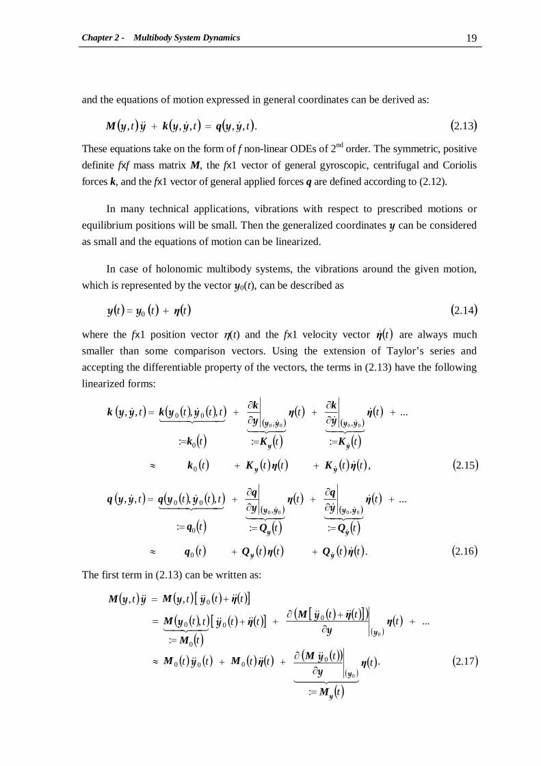
and the equations of motion expressed in general coordinates can be derived as:
These equations take on the form of f non-linear ODEs of 2nd order. The symmetric, positive
definite fxf mass matrix M, the fx1 vector of general gyroscopic, centrifugal and Coriolis
forces k, and the fx1 vector of general applied forces q are defined according to (2.12).
In many technical applications, vibrations with respect to prescribed motions or
equilibrium positions will be small. Then the generalized coordinates y can be considered
as small and the equations of motion can be linearized.
In case of holonomic multibody systems, the vibrations around the given motion,
which is represented by the vector y0(t), can be described as
where the fx1 position vector η(t) and the fx1 velocity vector ( )tη& are always much
smaller than some comparison vectors. Using the extension of Taylor’s series and
accepting the differentiable property of the vectors, the terms in (2.13) have the following
linearized forms:
The first term in (2.13) can be written as:
( ) ( ) ( ) ( )14.20 t tt η+= yy
( ) ( ) ( ) ( )13.2.,,,,, t t t yyyy y y &&&& qkM =+
( ) ( ) ( )( )( )
( )( )
( )( )( )
( )
( ) ( ) ( ) ( ) ( ) ( )
( ) ( ) ( )( )( )
( )( )
( )( )
( )( )
( ) ( ) ( ) ( ) ( ) ( )61.2.
...
:::
,,,,
51.2,
...
:::
,,,,
0
0
00
0
0
00
0000
0000
,,
,,
t t t t t
t
t
t
t
t
ttt t
t t t t t
t
t
t
t
t
ttt t
ηQηQq
η
Q
qη
Q
q
q
ηKηKk
η
K
kη
K
k
k
kk
&
&
43421&
4342144 344 21
&&
&
&
43421&
4342144 344 21
&&
&
&
&
&
&&
&&
yy
yy
yy
yy
yyyy
yyyy
yyyyyy
yyyyyy
++≈
+
=
∂∂+
=
∂∂+
=
=
++≈
+
=
∂∂+
=
∂∂+
=
=
( ) ( ) ( ) ( )[ ]( )( )( )
( ) ( )[ ] ( ) ( )[ ]( )( )
( )
( ) ( ) ( ) ( ) ( )( )( )
( )( ) ( )17.2.
:
...
:
,
,,
0
0
0000
00
0
0
0
t
t
t
tt tt
t tt
tt
t
tt
tt t t
η
M
MηMM
ηηMη
M
M
ηMM
44 344 21
&&&&&&
&&&&&&&&
43421
&&&&&&
y
y
y
yy y
yyy y
y y y y
=
∂∂++≈
+∂
+∂++=
=
+=
Chapter 2 - Multibody System Dynamics 20
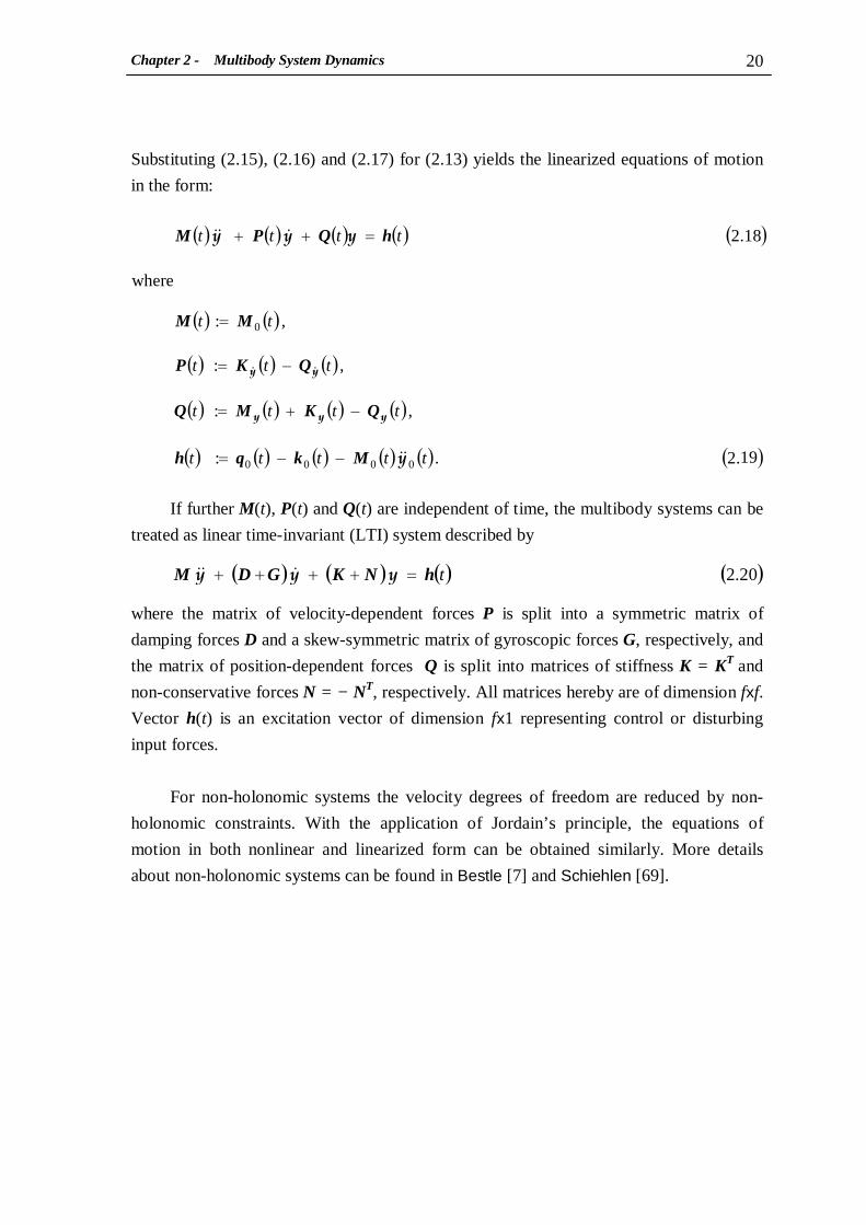
Substituting (2.15), (2.16) and (2.17) for (2.13) yields the linearized equations of motion
in the form:
If further M(t), P(t) and Q(t) are independent of time, the multibody systems can be
treated as linear time-invariant (LTI) system described by
where the matrix of velocity-dependent forces P is split into a symmetric matrix of
damping forces D and a skew-symmetric matrix of gyroscopic forces G, respectively, and
the matrix of position-dependent forces Q is split into matrices of stiffness K = KT and
non-conservative forces N = − NT, respectively. All matrices hereby are of dimension fxf.
Vector h(t) is an excitation vector of dimension fx1 representing control or disturbing
input forces.
For non-holonomic systems the velocity degrees of freedom are reduced by non-
holonomic constraints. With the application of Jordain’s principle, the equations of
motion in both nonlinear and linearized form can be obtained similarly. More details
about non-holonomic systems can be found in Bestle [7] and Schiehlen [69].
( ) ( ) ( ) ( ) ( )
( ) ( )( ) ( ) ( )( ) ( ) ( ) ( )( ) ( ) ( ) ( ) ( ) ( )19.2.:
,:
,:
,:
where
18.2
0000
0
tt t t t
t t t t
t t t
t t
t t t t
y
yy y
yyy
yy
&&
&&&
&&
Mkqh
QKMQ
QKP
MM
hQPM
−−=
−+=
−=
=
=++
( ) ( ) ( ) ( )20.2 t hNKGDM =++++ y y y &&&

Chapter 3 - Passenger Car Modeling 21
Chapter 3
Passenger Car Modeling
In this chapter, a spatial car model for a vehicle with a double-control-arm suspension
will be developed. The yaw motion of the car will be derived from a plane track model.
The linearized equations of motion obtained from the computer-aided multibody system
program NEWEUL will be transformed into the state-space representation form. Finally,
a simplified spatial car model will be presented which will be used to design optimal
control.
3.1 Suspension Forces
The influences of suspension geometry are often ignored in conventional quarter-car
models. In this section, modified suspension parameters characterizing the effects of
suspension geometry will be defined by comparing the virtual works generated by the
forces acting on the car body of a double-control-arm suspension and those of a
conventional quarter-car model. The virtual-work method introduced in this section can
be applied analogously for other types of suspension to find properly modified suspension
parameters.
3.1.1 Double-control-arm suspension
The schematic diagram of a double-control-arm suspension system is shown in Figure
3.1. In this model, the directions of the spring-damper and the actuator at the static
equilibrium are described by angles φ0 and φC0 respectively, while that of the lower

Chapter 3 - Passenger Car Modeling 22
control arm is presented by angle ξ0. The model has two degrees of freedom, the vertical
displacement of the sprung mass zS and the displacement of the unsprung mass which may
be represented by the rotational angle ξ of the lower suspension arm.
The given parameters of the model are the stiffness of the spring k0, the damping
coefficient of the damper b0, the rotational stiffness of the anti-roll bar r0 and positions of
joints. The suspension forces acting on the car body (sprung mass) result from spring,
damper, actuator and anti-roll bar.
• Spring and damping forces
Figure 3.2 illustrates the definition of the spring force vector FK and the damping force
vector FB when joint D connecting the spring-damper with the lower control arm moves to
D’. For small rotational angle ξ, i.e. ξ << 1, vector δD representing the displacement of joint
Figure 3.1: Plane model of double-control-arm suspension
ξ0
ϕ0
zS
lD
lA
S
zS
yS
k0
b0
r0
anti-roll bar
ξ
lE
lC
ϕC0
actuator
A C D E
U
O

Chapter 3 - Passenger Car Modeling 23
D can be treated to be orthogonal to the lower control arm OD and its value can be
defined by δD = lD sin(ξ) ≈ lD ξ, resulting in the dynamic deflection of the spring-damper:
The spring force FK is proportional to the sum of dynamic deflection ∆l and static
deflection ∆l0 of the spring, i.e.
The damping force FB can be computed approximately by
Figure 3. 2: Definition of the spring and damping forces
( ) ( ) ( )1.3.sinsin 00 l l ϕξϕδ DD ≈≈∆
( ) ( )( )
( ) ( )3.3.sin
:3.1or with
2.3,
0000
00
lk lk F
l lk F
∆+=
∆+∆=
ϕξDK
K
( ) ( )4.3.sin 000 lb lb F ϕξ&&DB =∆=
δϑ
ξ0
lD D
S
zS
FK
D’
yS
ϕ0 ξ
zS
0ϑ
FB
δD O

Chapter 3 - Passenger Car Modeling 24
By defining an instantaneous velocity center P of the unsprung mass as shown in
Figure 3.3, the rotational angle ξ and velocity ξ& of the lower suspension arm can be
expressed by
respectively, where ∆z = ( zU – zS ) is the relative vertical displacement between the sprung
and unsprung mass. Substituting ξ into Equation (3.3) yields
With ξ& defined by (3.6), the damping force FB in (3.4) can be expressed by
In the above, λD is the coefficient representing the influences of the suspension geometry
on the spring and damping forces.
∆z = zU – zS
lD D
U
LU
P
LE
ξ
∆z/cos(χ0)
instantaneous velocity center
E
D’ E’
χ0
δD
lE
O
( )
( )6.3,
and
5.3
z Ll
L
z Ll
L
&& ∆≈
∆≈
UE
E
UE
E
ξ
ξ
Figure 3. 3: Definition of the rotational angle of the lower suspension arm
( ) ( )7.3.
:
sin 0000 l k z Ll
Ll k F ∆+∆
=
=44 344 21
D
UE
EDK
λ
ϕ
( )8.3.0 z b F &∆= DB λ

Chapter 3 - Passenger Car Modeling 25
By introducing rotational matrices ( )δϑϑ +00 and , SSS ξξ corresponding to angles ξ0, ξ and ( )δϑϑ +0 as
and 1<<δϑ , the directional unit vector eD of FK and FB in the
coordinate system S fixed to the sprung mass can be defined by
while vector δD in the coordinate system S can be defined from vectors rOD and rOD’ as
( )
( ) ( )( ) ( )
( )14.3
cossin
sincos
0
0
0
with
13.3
00
00'
'
0
l l
+−+=
=
−=
ξξξξξξDDOD
ODODD
ξξ SSr
rrδ
( ) ( )( ) ( )
( )
( ) ( )( ) ( )
( )
( ) ( ) ( )( ) ( )
( )11.3
cossin0
sincos0
001
10.3,
10
10
001
cossin0
sincos0
001
9.3,
cossin0
sincos0
001
00
00
00
00
0
0
+++−+=
−≈
−=
−=
+
δϑϑδϑϑδϑϑδϑϑ
ξξ
ξξξξ
ξξξξ
δϑϑS
S
S
ξ
ξ
( )000 2
: where ξϕπϑ +−=
( ) ( )( )
( ) ( )( ) ( )
( )12.3
sincos
cossin
0
cos
sin
0
1
0
0
00
00
0
00
+−+≈
+−+=
−= +
δϑϑϑδϑϑϑ
δϑϑδϑϑδϑϑSeD
( )( )
( )15.3
sin
cos
0
0
0
and
0
00 l l
−=
=
ξξDDOD ξSr

Chapter 3 - Passenger Car Modeling 26
resulting in
With the directional unit vector eD (3.12), the vector of spring force FK can be defined as
The virtual work generated by the spring force can be computed by
Substituting (3.16) and (3.17) into (3.18) and taking into account 1, <<δϑξ yields
Similarly, the virtual work generated by the damping force can be computed by
The virtual works generated by the spring and damping forces of the double-control
arm suspension model will be compared to those of a conventional quarter-car model to
define the modified suspension stiffness and damping coefficient.
( )( )
( )16.3.
cos
sin
0
0
0 l
=
ξξξDDδ
( ) ( )( ) ( )
( )( )
( )( )
( )17.3.
sin
cos
0
cos
sin
0
sincos
cossin
0
0
0
0
0
00
00
F F
F F
δϑϑϑ
ϑϑ
δϑϑϑδϑϑϑ
+
−=
+−+==
KK
KDKK eF
( )18.3. W DTKK δF=δ
( )21.3.20 z z b W ∆∆−= &DB λδ
( )( )( ) ( )
( ) ( )( ) ( )02.3.
:7.3and
3.5 withor
19.3,sin
2coscos
002
0
0
000
z l k z k z F W
l F
lF lF W
∆∆+∆−=∆−=
−=
−−=+−==
DDDKK
DK
DKDKDTKK δF
λλλδ
ϕξ
ϕπξξϑξδ
Chapter 3 - Passenger Car Modeling 27
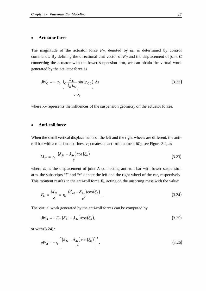
• Actuator force
The magnitude of the actuator force FC, denoted by u0, is determined by control
commands. By defining the directional unit vector of FC and the displacement of joint C
connecting the actuator with the lower suspension arm, we can obtain the virtual work
generated by the actuator force as
where λC represents the influences of the suspension geometry on the actuator forces.
• Anti-roll force
When the small vertical displacements of the left and the right wheels are different, the anti-
roll bar with a rotational stiffness r0 creates an anti-roll moment MU, see Figure 3.4, as
where δA is the displacement of joint A connecting anti-roll bar with lower suspension
arm, the subscripts “l” and “r” denote the left and the right wheel of the car, respectively.
This moment results in the anti-roll force FU acting on the unsprung mass with the value:
The virtual work generated by the anti-roll forces can be computed by
( ) ( ) ( )23.3cos 0
0 e
r M
ξδδ ArAlU
−=
( ) ( )22.3
:
sin 00 z Ll
Ll u W ∆
=
−=44 344 21
C
CUE
ECC
λ
ϕδ
( ) ( ) ( )24.3.cos
20
0 e
r
e
MF
ξδδ ArAlUU
−==
( ) ( ) ( )
( ) ( ) ( )26.3.cos
:(3.24)or with
25.3,cos
20
0
0
e
r W
F W
−−=
−−=
ξδδδ
ξδδδ
ArAlA
ArAlUA

Chapter 3 - Passenger Car Modeling 28
For small rotational angle ξ of the lower control arm, the displacement δA can be
computed from Figure 3.4a as
Figure 3.4: Definition of the anti-roll force
( )( )
( )28.3.
:53.in given or with
27.3,
z Ll
L l
l
∆≈
≈
UE
EAA
AA
δ
ξξδ
δAl cos(ξ0)
e 2a
2c
FA
FU
FU
FA
b)
A B
z
y x
a)
ξ0
zS
lA
U
LU
S
zS
P
lE
ξ δA
yS
FA
A
A’
∆z = zU – zS
zU
FU
MU
LE
r0
E
E’
B
δAr cos(ξ0)

Chapter 3 - Passenger Car Modeling 29
Substituting the above equation into (3.24) and (3.26) yields
where λA is the coefficient representing the influences of the suspension geometry on the
anti-roll forces. At the sprung mass, the value of the anti-roll force FA is defined by the
equilibrium condition
3.1.2 Modified suspension parameters
Let us consider the conventional quarter car model illustrated in Figure 1.3 with spring
stiffness k, the damping coefficient b and the value u of the actuator force FC. For this
model, the values of the spring force FK with pre-stress 0ˆKF and damping force FB are
defined by
where zU and zS are vertical displacements of unsprung and sprung mass, respectively.
Since the directions of the forces acting on the bodies and displacements are opposite,
the virtual works resulting from the spring, damper and control force can be computed as
( ) ( ) ( )
( ) ( ) ( )30.3
:
cos1
29.3,cos1
22
00
020
z z
Ll
Ll
e r W
z z Ll
Ll
e r F
rl
A
UE
EAA
rlUE
EAU
∆−∆
=
−=
∆−∆=
444 3444 21
λ
ξδ
ξ
( )
( )32.3.
in resulting
31.3022
0 c e
a r
c
aF F
c
F
a
F
AUA
AU
λ==
=−
( ) ( )( )( )37.3.
36.3,
35.3,ˆ0
z u W
z
z b
z F
W
z F
z k
z F W
∆−=
∆∆−=∆−=
∆+∆−=∆−=
C
BB
KKK
δ
δ
δ
&
( ) ( )( ) ( )34.3:
33.3,ˆ:ˆ00
z b zz b F
F
z k
F
zz k F
&&& ∆=−=
+∆=+−=
SUB
KKSUK

Chapter 3 - Passenger Car Modeling 30
Comparing the above virtual works to those of the double-control-arm model defined by
(3.20), (3.21) and (3.22), respectively, yields
For a half-car or full-car model constructed from a combination of quarter car models,
the value of the anti-roll force FA at the left and the right wheel can be computed by
resulting in the virtual work
where r is the modified rotational stiffness of the anti-roll bar. Comparing to the virtual
work (3.30) yields the anti-roll stiffness for a simplified car model:
It should be noted that the unit of r is [N/m/rad] instead of [Nm/rad] due to the unit of
λA (3.30).
With the modified suspension parameters defined by (3.38), (3.39), (3.40) and
(3.43), the influences of the geometry of a double-control-arm suspension can be involved
in the conventional simplified car models.
( )43.3.20 r r Aλ=
( ) ( )41.3 zz r F rlA ∆−∆=
( )( )( )40.3.
39.3,
38.3,ˆ,
0
20
002
0 0
u u
b
b
l kF k k
C
D
DKD
λ
λ
λλ
=
=
∆==
( ) ( ) ( )42.32 zz r zz F W rlrlAA ∆−∆−=∆−∆−=δ
Chapter 3 - Passenger Car Modeling 31
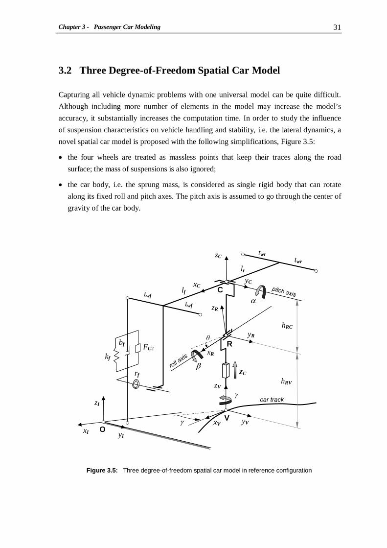
3.2 Three Degree-of-Freedom Spatial Car Model
Capturing all vehicle dynamic problems with one universal model can be quite difficult.
Although including more number of elements in the model may increase the model’s
accuracy, it substantially increases the computation time. In order to study the influence
of suspension characteristics on vehicle handling and stability, i.e. the lateral dynamics, a
novel spatial car model is proposed with the following simplifications, Figure 3.5:
• the four wheels are treated as massless points that keep their traces along the road
surface; the mass of suspensions is also ignored;
• the car body, i.e. the sprung mass, is considered as single rigid body that can rotate
along its fixed roll and pitch axes. The pitch axis is assumed to go through the center of
gravity of the car body.
Figure 3.5: Three degree-of-freedom spatial car model in reference configuration
R
zR
θ yR
yC
zC
xC C
xR
α
β zC
V
zV
yV xV
kf
bf FC2
γ
rf hRV
hRC
yI
zI
xI γ
twf
twf
lf
lr
twr
twr
O

Chapter 3 - Passenger Car Modeling 32
The spatial car model has three degrees of freedom: 1) the vertical motion
expressed by zC, 2) the rotational motion β about the roll axis which is inclined by a
constant angle θ with respect to the horizontal axis, and 3) the rotational motion about the
pitch axis denoted by pitch angle α . In order to describe the motion of the car body, three
coordinate systems are introduced additionally to the absolute inertial reference frame
{ O, xI, yI, zI }, i.e. the track coordinate system {V, xV, yV, zV }, the car body roll motion
coordinate system {R, xR, yR, zR } and the car body fixed coordinate system {C, xC, yC, zC }.
The direction of coordinate systems is defined according to ISO 8855, i.e. the positive x-
axis points straight forward, the y-axis points to the left and the z-axis points upwards.
The trace of the chassis, i.e. the un-sprung mass including the four wheels, in the x-y
plane of the reference frame O can be described with a coordinate system that translates
only within the x-y plane and rotates only along the zI-axis. This coordinate system is
referred to as the track coordinate system V. At equilibrium of the car, the z-axis of V runs
through the center of gravity of the car body. It is obvious that the rotation of V represents
the yaw motion of the car denoted by γ.
The roll motion coordinate system R is assumed to keep its origin directly above the
coordinate system V, i.e. R shifts only along the z-axis of V. This shifting is indicated by
zC and it is one of the three degrees of freedom of the car body. Orientation of system R
can be described by two consequent elementary rotations. The first one is a rotation about
the y-axis of coordinate system V with a fixed angle θ defining the roll axis of the sprung
mass. The consequent rotation is about the x-axis of frame R with roll angle β which
along with the rotation axis describes the roll motion of the sprung mass and yields the
second degree of freedom of the car body.
The last coordinate system C is fixed to the car body with its origin fixed to
coordinate system R and a rotational degree about the y-axis. This rotation represents the
pitch motion of the car and is characterized by angle α, which is the third degree of
freedom of the car body.
Applied forces and moments on the car body result from springs, dampers and
actuators of the four suspensions and anti-roll bars in the front and at the rear side of the car.

Chapter 3 - Passenger Car Modeling 33
3.3 Plane Track Model
The car is assumed to move along a given trajectory and to keep its yaw orientation
tangential to the track all the time. In order to describe the motion of the car, the track
must be modeled first. A relatively simple and easy way to produce a car track is the
division of the whole track path into sections. It is possible to reproduce all road courses
which occur in real road systems using only three different path forms: straight-line, spiral
and circular-arc segments as illustrated in Figure 3.6.
The track is described by a track coordinate s along the track and its curvature
κ = κ(s) which is the inverse of the curve radius R(s), i.e. |κ(s)| = 1/R(s), where κ(s) > 0 for
a left curve and κ(s) < 0 for a right curve. The curvature of the track segments can be
defined as follows:
Figure 3.6: Basic path forms of the track
xI
yI
R = R0
R → ∞
R = R(s)
s
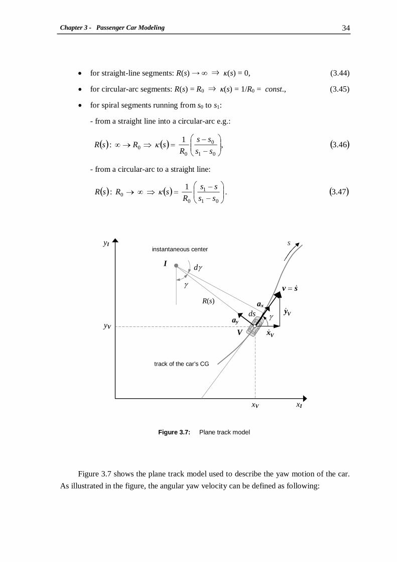
Chapter 3 - Passenger Car Modeling 34
• for straight-line segments: R(s) → ∞ ⇒ κ(s) = 0, (3.44)
• for circular-arc segments: R(s) = R0 ⇒ κ(s) = 1/R0 = const., (3.45)
• for spiral segments running from s0 to s1:
- from a straight line into a circular-arc e.g.:
- from a circular-arc to a straight line:
Figure 3.7 shows the plane track model used to describe the yaw motion of the car.
As illustrated in the figure, the angular yaw velocity can be defined as following:
Figure 3.7: Plane track model
( ) ( ) ( )3.46 ,1
:01
0
00
ss
ss
R s R sR
−−=⇒→∞ κ
( ) ( ) ( )3.47 .1
:01
1
00
ss
ss
R s R sR
−−=⇒∞→ κ
xI
I
xV
yV
yI
track of the car’s CG
R(s)
V
sv &=
ay
ax
γ
instantaneous center s
γ dγ
Vx&
Vy&ds

Chapter 3 - Passenger Car Modeling 35
The trajectory of the track in the x-y plane of the inertial coordinate system may be
computed from
The accelerations VV yx &&&& and can be projected along tangent and normal directions of the
moving frame V as
Alternatively the car longitudinal and lateral acceleration can be calculated from longitudinal
and angular velocity as
3.4 Linearized Equations of Motion of the Spatial Car Model
In this section, the linearized equations of motion of the spatial car model will be defined
which will be used for simulation and control analysis. As indicated in section 3.2, the
vector of generalized coordinates for the spatial car model may be chosen as
y := [ zC , β , α ] T (3.52)
and the vector of general applied forces and moments resulting from the suspension and
expressed in the car body fixed frame may be summarized as
qa := [ fzC , lβ , lα ] T . (3.53)
( ) ( )[ ] ( )3.51 .
,
2
v s v v sR
v a
va
γκ &
&
===
=
y
x
( ) ( ) ( ) ( )3.48 .11
v sssRdt
ds
sRdt
d κγγ ==== &&
( )( ) ( )3.49.sin
, cos
v y
v x
γ
γ
V
V
=
=
&
&
( ) ( )( ) ( ) ( )3.50.cossin
,sincos
y x a
y x a
γγ
γγ
VVy
VVx
&&&&
&&&&
+−=
+=

Chapter 3 - Passenger Car Modeling 36
More details about these quantities will be given in Section 3.5. It is assumed that the car
body roll and pitch angles are small, i.e. β, α <<1. This assumption is acceptable since the
maximum value of the roll angle for passenger cars in typical rollover test maneuvers is
less than 6 degrees, Forkenbrock, et al. [26], Ungoren, et al. [79, 80, 81] and Viano and
Parenteau [85], in addition the pitch motion is often neglected for even roads and normal
maneuvers, i.e. without sudden acceleration. Based on the theoretical derivation in
Chapter 2, the computer-aided multibody system program NEWEUL can be applied
resulting in the linearized equations of motion
of the spatial car model where the mass matrix M is given as
( )54.3
hQPM =++ yyy &&&
( ) ( ) ( ) ( )
( ) ( )( ) ( )
( )
( ) ( )( ) ( ) ( ) ( )
( ) ( ) ( )
( )
( ) ( ) ( ) ( )( ) ( )58.3
. sincossincos
by drepresente is and
57.3 ,
cos0
coscos
cossin0
000
as dsrea the
56.3
,
0cos0
cos00
000
is the
55.3,
00
0sincos0
00
2
222
222
+++=
−−−−
−−−+−
−=
−+−+−=
++=
α
β θαθθγθ
γθγ
θγθγ
θθ
θγθγ
θθ
l
lIahm
fz
forces excitation of vector the
II
II
II IIhm
ahm
forces dependent-position of matrix
III
III
forces dependent-velocity of matrix
I
I Ihm
m
&&
&&&
&&
&
&
&
ZyRCS
C
ZXZX
ZX
ZYRCS
xRCS
ZYX
ZYX
Y
ZXRCS
S
h
Q
P
M

Chapter 3 - Passenger Car Modeling 37
The physical meaning and values of the symbols in the equations above and the
NEWEUL output file are provided in Appendices A and B, respectively.
The vector of excitation forces h can be divided into two components
where the first term hw denotes the excitation by exogenous disturbances resulting from
the yaw motion of the car which generates the lateral acceleration ay and the yaw
accelerationγ&& . Summarizing these quantities in a vector of disturbances w yields
The second term q in Equation (3.59) is the vector of general applied forces, which is
related to vector (3.53) by
Using the equations (3.59), (3.60) and (3.61), the linearized equations of motion of
the spatial car model (3.54) can be rewritten as
( )3.62 . aqGwHQPM qwα+=++ y y y &&&
( ) ( ){
( )60.3
.
::
00
sincos
00
a
Ihm
wH
hy
w
ZRCSw
=
=
=
γθθ
&&4444 34444 21
( ) ( )( ) ( )61.3 .
:
100
0sincos0
001
a
q
q
G
q
44444 344444 21
α
θαθ
=
+=
( ) ( ) ( ) ( )( ) ( )59.3
:
sincos
:
0
sincos
0
l
l
fz
Iahm
=
+
+
=
+
=
444 3444 2144444 344444 21
&&
qh
h
C
w
ZyRCS
α
β θαθθγθ
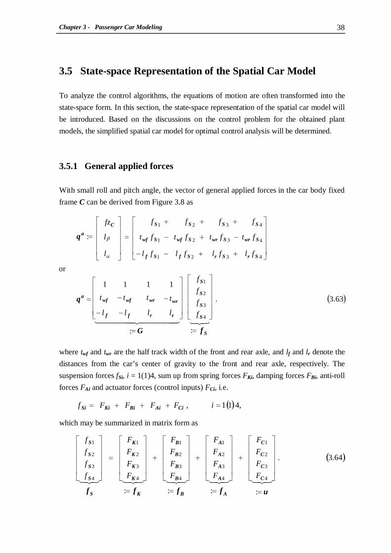
Chapter 3 - Passenger Car Modeling 38
3.5 State-space Representation of the Spatial Car Model
To analyze the control algorithms, the equations of motion are often transformed into the
state-space form. In this section, the state-space representation of the spatial car model will
be introduced. Based on the discussions on the control problem for the obtained plant
models, the simplified spatial car model for optimal control analysis will be determined.
3.5.1 General applied forces
With small roll and pitch angle, the vector of general applied forces in the car body fixed
frame C can be derived from Figure 3.8 as
where twf and twr are the half track width of the front and rear axle, and lf and lr denote the
distances from the car’s center of gravity to the front and rear axle, respectively. The
suspension forces fSi, i = 1(1)4, sum up from spring forces FKi, damping forces FBi, anti-roll
forces FAi and actuator forces (control inputs) FCi, i.e.
which may be summarized in matrix form as
( ) ,411, i F F F F f =+++= CiAiBiKiSi
( )64.3.
::::
4
3
2
1
4
3
2
1
4
3
2
1
4
3
2
1
4
3
2
1
F
F
F
F
F
F
F
F
F
F
F
F
F
F
F
F
f
f
f
f
=
+
=
+
=
+
=
=
321321321321321
uffff
C
C
C
C
A
A
A
A
A
B
B
B
B
B
K
K
K
K
K
S
S
S
S
S
( )3.63 .
::
1111
or
:
4
3
2
1
4321
4321
4321
f
f
f
f
l l ll
tt tt
fl
fl
fl
fl
ft ft ft
ft
f
f
f
f
l
l
fz
32144444 344444 21
S
S
S
S
S
rrff
wrwrwfwfa
SrSrSfSf
SwrSwrSwfSwf
SSSSC
a
fG
q
q
=
=
−−−−=
++−−−+−+++
=
=
α
β

Chapter 3 - Passenger Car Modeling 39
It should be noted that the static spring forces cancel against the weight of the vehicle and
will not be considered in the following.
Since the four wheels of the car are assumed to be mass-less points keeping their
traces on the road surface, i.e. zUi = 0, the vector of spring forces can be computed only
from the vertical displacements zSi of the nodal points Si according to section 3.1.2 by
the damping forces by
and the anti-roll forces by
( )65.3,
::
000
000
000
000
4
3
2
1
z
z
z
z
k
k
k
k
321444 3444 21
S
S
S
S
S
S
r
r
f
f
K
zK
f
=
=
−=
( )
z
z
z
z
b
b
b
b
66.3
::
000
000
000
000
4
3
2
1
321
&
&
&
&
&
444 3444 21
S
S
S
S
S
S
r
r
f
f
B
zB
f
=
=
−=
Figure 3.8: Applied forces and moments in the car body fixed frame
lf
lr
S2
S1
S3
S4
lα
zC
yC
xC C
lβ
twf
twf
twr
twr
fzC
fS2
fS1
fS3
fS4

Chapter 3 - Passenger Car Modeling 40
where kf and kr are the translational stiffnesses of the front and rear suspensions, bf and br are
the damping coefficients of the front and rear suspensions, and rf and rr are the rotational
stiffnesses of the front and rear anti-roll bars, respectively. With the above equations, the
vector of total suspension forces fS in Equation (3.64) can be expressed as a function of vertical
displacements zS and velocitiesSz& of the suspension nodes attached to the sprung mass as
For small roll and pitch angles, the linearized relations between the vertical displacements
of the suspension nodes zSi, i = 1(1)4, and the generalized coordinates can be defined from
Figure 3.9 as
Due to the constant matrix TSG , the relation betweenSz& and y& reads as
Using equations (3.63) and (3.68) − (3.70) results in the vector of general applied
forces in the car body fixed frame C:
( )( )( )( )
( )( )( )( )
{
( )3.69 .
:
cos1
cos1
cos1
cos1
notationmatrix in or
cos
, cos
, cos
, cos
4
3
2
1
4
3
2
1
z
l t
l t
lt
lt
z
z
z
z
l t z z
l t z z l t z z
l t z z
y
=
−
−−−
=
+−=++=−−=−+=
αβ
θθθθ
αθβαθβαθβαθβ
C
TS
rwr
rwr
fwf
fwf
S
S
S
S
S
rwrCS
rwrCS
fwfCS
fwfCS
Gz4444 34444 21321
( ) ( )68.3. uzBzKKf SSSASS +−+−= &
( )67.3
::
00
00
00
00
4
3
2
1
z
z
z
z
rr
rr
rr
rr
3214444 34444 21
S
S
S
S
S
A
rr
rr
ff
ff
A
zK
f
=
=
−−
−−
−=
( )70.3. y &&TSS Gz =
( )[ ] ( )71.3. uGBGKKGq TSS
TSAS
a +−+−= y y &

Chapter 3 - Passenger Car Modeling 41
Substitution of qa in (3.71) with linearization due to 1,,, <<uy y & α yields a final
representation of the vector of general applied forces (3.61) in inertial system:
( )[ ]( ) ( )( )
( )[ ]
( ) ( ) ( ) ( )
( ) ( )[ ]
( )[ ] ( )72.3
1111
sin
coscoscoscos
1111
1111
100
0sincos0
001
l l ll
tt tt
l l ll
tt tt
l l ll
tt tt
uGBGKKG
uGBGKK
G
uGBGKK
uGBGKKGGq
TSS
TSASS
TSS
TSAS
rrff
wrwrwfwf
S
rrff
wrwrwfwf
TSS
TSAS
rrff
wrwrwfwf
TSS
TSASq
+−+−≈
+−+−
−−−−+
−−−−=
+−+−
−−−−
+=
+−+−=
y y
y y
y y
y y
&
&
4444444444 34444444444 21
&
&
θα
θθθθ
θαθ
α
Figure 3.9: Vertical displacements of the suspension nodes for small angles α and β
θ
lfα
twrβ
α
zC
yC
xC C
β
twrβ
lfα
lrα
lrα
twfβ twfβ
zC
zC
zC
zC
zS1 = zC + twfβ cos(θ )− lfα
zS2 = zC − twfβ cos(θ )− lfα
zS4 = zC − twrβ cos(θ )+ lrα
zS3 = zC + twrβ cos(θ )+ lrα
θ
θ
θ
θ
Chapter 3 - Passenger Car Modeling 42
where GS has been defined in Equation (3.69). The linearized equations of motion of the
spatial car model (3.62) finally can be expressed by
This equation will be used in the simulation process to calculate the quantities estimating
the dynamic characteristics of the spatial car model.
3.5.2 Linear parameter-varying spatial car model
In order to analyze and synthesize the control algorithms for the spatial car model, the
linearized equations of motion (3.73) must be transformed to state equations as
where [ ] [ ]TCCTTTx
z z αβαβ &&&& ,,,,,,: == yy is the state vector, ( )γ&&,yw a is the vector
of exogenous disturbances according to (3.60), and ( ) and,,, 4 66 6 x x RI RI ∈∈ BA x a γγ &&& 2 6 x RI∈wB are state matrices. The matrices ( ) ( ) ( ) ( )γγγ &&&& ,,:and: xQ.QP.P a == are the
parameter-dependent terms of the matrix ( )γγ &&&,,xA a and defined by (3.56) and (3.57),
respectively.
Let [ ] 5,,: RI∈= yzyTT
S β&& denote the vector of measured outputs and define the
relation , then with (3.69) and (3.73) the measurement
equations of the spatial car model can be written as
[ ] ( )[ ] ( )3.73 . uGwHGKKGQGBGPM SwTSASS
TSSS +=+++++ y y y &&&
( ) ( )[ ] ( )[ ]( )
( )74.3
::
:,,::
11
11
a
a
=
+
=
+
=
=+−++−
=
=
−−
−−
321&&
4342143421
321&
44444444444 344444444444 21
&&&
321
&
&&
&
wB
HM
0u
B
GM
0
xA
GBG.PMGKKG.QM
I0
x
y
w
wS
x
TSSS
TSASS
γ
γγ
y
y
y
y
[ ]0,1,0with ==TT gg βββ &&&&
&&&& y
Chapter 3 - Passenger Car Modeling 43
where ( ) 254 565 and,, , xxx a RI RI RI ∈∈∈ wx DDC γγ &&& are the measurement matrices.
Please note the difference in the symbols y for measurement output and y for generalized
coordinate.
With the state equations (3.74) and measurement equations (3.75), the equations of
motion of the spatial car model can be expressed in the state-space form of a linear
parameter-varying (LPV) system:
It should be pointed out that in general the varying parameters of the system can take any
values in some operation region, i.e. their time functions are unknown beforehand. Therefore,
the state-space matrices ( )γγ &&&,,xA a and ( )γγ &&&,,xC a and the vector of disturbances ( )γ&&,yw a are treated as on-line data. The variations of the system parameters result in the changes
of system dynamics. To maintain the required performance of the system, a parameter-
varying controller must be designed which is able to update its parameters on-line
according to the variations of the system parameters. However, for systems with more than
two varying parameters, it is very difficult to design such a controller, Balas, et al. [5],
Fitzpatrick [25], Gaspar, et al. [29] and Wu [93]. Therefore, the spatial car model must be
simplified in order to reduce the number of system varying parameters.
( ) ( )( ) ( )
( )76.3
.,,,
,,,,
a a
a a
++=
++=
γγγ
γγγ
&&&&&
&&&&&&
ywx
ywx
wDuDxCy
wBuBxAx
{
( ) ( )[ ] ( )[ ]( )
{
{
( )75.3
::
,,:
11
11
a
a
=
+
=
+
=
+−++−=
−−
−−
wD
HMg
0u
D
GMg
0
x
C
GBG.PMgGKKG.QMg
0G
y
z
y
w
wT
ST
x
TSSS
TTSASS
T
TSS
γ
γγβ
ββ
ββ
&&44344214434421
&4444444444444 34444444444444 21
&&&
&&
&&&&
&&&& y
y
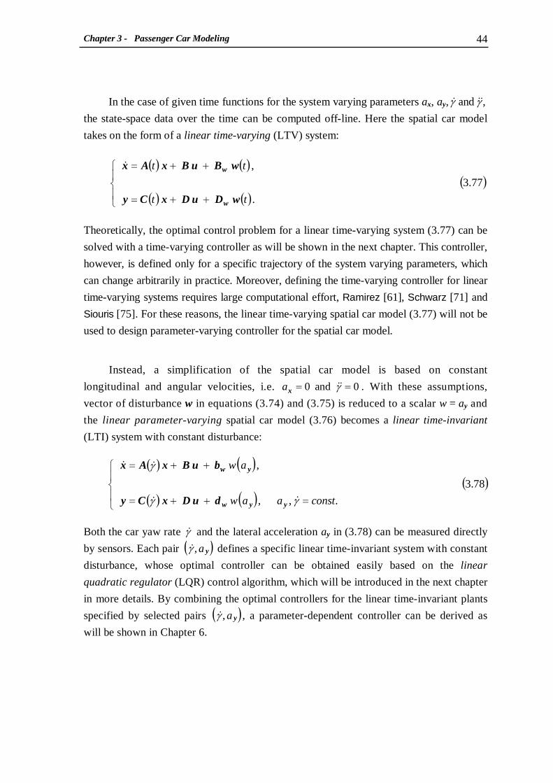
Chapter 3 - Passenger Car Modeling 44
In the case of given time functions for the system varying parameters ax, ay, , andγγ &&&
the state-space data over the time can be computed off-line. Here the spatial car model
takes on the form of a linear time-varying (LTV) system:
Theoretically, the optimal control problem for a linear time-varying system (3.77) can be
solved with a time-varying controller as will be shown in the next chapter. This controller,
however, is defined only for a specific trajectory of the system varying parameters, which
can change arbitrarily in practice. Moreover, defining the time-varying controller for linear
time-varying systems requires large computational effort, Ramirez [61], Schwarz [71] and
Siouris [75]. For these reasons, the linear time-varying spatial car model (3.77) will not be
used to design parameter-varying controller for the spatial car model.
Instead, a simplification of the spatial car model is based on constant
longitudinal and angular velocities, i.e. 0and0 == γ&& ax . With these assumptions,
vector of disturbance w in equations (3.74) and (3.75) is reduced to a scalar w = ay and
the linear parameter-varying spatial car model (3.76) becomes a linear time-invariant
(LTI) system with constant disturbance:
Both the car yaw rate γ& and the lateral acceleration ay in (3.78) can be measured directly
by sensors. Each pair ( )ya,γ& defines a specific linear time-invariant system with constant
disturbance, whose optimal controller can be obtained easily based on the linear
quadratic regulator (LQR) control algorithm, which will be introduced in the next chapter
in more details. By combining the optimal controllers for the linear time-invariant plants
specified by selected pairs ( )ya,γ& , a parameter-dependent controller can be derived as
will be shown in Chapter 6.
( ) ( )( ) ( )
( )77.3
.
,
t t
t t
++=
++=
wDuDxCy
wBuBxAx
w
w&
( ) ( )( ) ( )
( )78.3
.,,
,
const
a
aw
aw
=++=
++=
γγ
γ
&&
&&
yyw
yw
duDxCy
buBxAx

Chapter 3 - Passenger Car Modeling 45
3.6 Simulation Model of the Spatial Car
In order to calculate the quantities estimating the dynamic characteristics of the spatial car
model, a simulation model is built in MATLAB/Simulink, Moscinski and Ogonowski [52],
where the spatial car model is combined with the optimal state-feedback and disturbance-
feed forward controllers, Figure 3.10.
Since the varying parameters of the spatial car model can be computed from the car
longitudinal velocity v and track curvature κ by equations (3.48) and (3.51), these
parameters are defined as the input parameters for the simulation and generated in the
block ‘Maneuvers’. By changing the time-behaviour of the car longitudinal velocity and
track curvature, different operation regimes of the car are simulated. The linearized
equations of the spatial car model (3.74) are solved in block ‘Spatial Car Model’ by a
MATLAB S-function which is presented in Appendix C. The measured outputs and
dynamic criteria specified for the spatial car model are defined in block ‘Criteria’. The
optimal control law with state-feedback and disturbance-feed forward is structured in
block ‘Controller’. Here the control forces are computed. For the passive suspension case,
the controllers are initialized with zero matrices. To observe lively the simulation process,
the movement of the car is animated by block ‘Animation’.
Figure 3.10: Simulation model of the spatial car model in MATLAB/Simulink
Chapter 4 - Linear Quadratic Regulator Control 46
Chapter 4
Linear Quadratic Regulator Control
Linear quadratic regulator control (LQR) is a powerful concept of optimally controlling
linear systems whose states are available to be fed back, i.e. the states can be measured
online. In this chapter, the LQR problem is shown for linear systems without disturbances
which results in an optimal state-feedback controller, and then extended to linear systems
with measurable disturbances, which leads to an optimal disturbance-feed forward
controller. The difficulty of solving the differential Riccati equation (DRE) for the case of
linear time-varying (LTV) systems will be exposed. In contrast to the case of linear time-
varying systems, the solutions of the LQR problem for linear time-invariant (LTI) systems
can be easily obtained by solving the algebraic Riccati equation (ARE). The LQR control
design based on the automotive performance criteria specified for the spatial car model will
demonstrate the effect of LQR control to passenger cars with active suspensions.
4.1 LQR Problem for Linear Systems without Disturbances
In this section, the standard LQR problem is defined and solved based on Pontryagin’s
maximum principle to find the optimal controller for linear systems without disturbances.
This method will be applied to linear systems with measurable disturbances in the next
section to define an optimal controller for the spatial car model.

Chapter 4 - Linear Quadratic Regulator Control 47
4.1.1 Definition of the LQR problem
In the case of vanishing disturbances w(t) = 0, the linear time-varying spatial car model
(3.77) becomes a special case of the general linear time-varying system of the form
where ( ) ( ) ( ) umn uyx RIRIRI ∈∈∈ ttt ,, are vectors of states, measured outputs and control
inputs, respectively; ( ) ( ) unnn BA x x tt RIRI ∈∈ and are state matrices while ( ) nmC x t RI∈
( ) umD x t RI∈ and are the measurement matrices. The LQR problem is to find a control input
u(t) minimizing the following quadratic objective function subject to constraints (4.1):
The matrix ( ) nnQ x t RI∈ is symmetric and positive semi-definite, i.e. Q(t) = Q(t)T ≥ 0,
weighting the states while( ) uuR x t RI∈ is a symmetric positive definite matrix, R(t) = R(t)T > 0,
penalizing the control effort. The mix-relation between the states and control inputs
denoted by the matrix ( ) unN x t RI∈ will be shown later in Equation (4.4).
Relatively small elements of Q(t) compared to R(t) will result in a control law which
will tolerate large errors in the states with low inputs. On the other hand, if Q(t) is made large
compared to R(t), this will result in tight control, i.e. small errors in the states with
considerable inputs. Different values of the entries of Q(t) or R(t) can be used to penalize
specific states compared to others at the same expense of control energy. In the standard LQR
problem the matrix R(t) is assumed to be positive definite, however, the special case R(t) = 0
of the LQR problem called the singular problem can be found in Moylan and Moore [53],
Ramirez [61] and Schwarz [71].
In most optimization problems, the objectives that need to be regarded for
minimization are not the complete state vector x(t) but only a selection according to
measurement outputs y(t). Therefore, the objective function (4.2) may be replaced by
( ) ( ) ( ) ( )[ ] ( )2.4.2:,,00
dt t t t dt t J ∫∫ ∞∞
++== uRuuNxxQxxu TTT��
( ) ( ) ( )( ) ( )
( )1.4
,0, 0
t t
t t
+=
=+=
uDxCy
xxuBxAx&
( ) ( )[ ] ( )3.4.0
dt t t J ∫∞ += uRuyQy uT
yT

Chapter 4 - Linear Quadratic Regulator Control 48
where ( ) ( ) ( ) ( ) ( ) ( ) 0, and0, >=∈≥=∈ Tuu
uuu
Tyy
mmy RRR QQQ tt ttt t x x RIRI are
weighting matrices of the measured outputs and controlled inputs, respectively.
Substitution of y(t) from (4.1) in (4.3) yields
The equation shows that the objective function J defined in (4.3) is contained in the more
general form (4.2) with properly defined matrices Q(t), N(t), and R(t). The assumptions of
Qy(t) ≥ 0 and Ru(t) > 0 ensure the conditions of Q(t) ≥ 0 and R(t) > 0 to hold for any C(t)
and D(t).
4.1.2 LQR solution using the Pontryagin’s maximum principle
There are different techniques to solve the LQR problem. In this section, the solution of
the LQR problem will be deduced from Pontryagin’s maximum principle. Pontryagin’s
maximum principle states that the optimal control u(t) that minimizes the objective
function (4.2) subject to constraint (4.1) must minimize the so-called Hamiltonian
where ( ) nλ RI∈t are the dynamic Lagrange multipliers or co-state vector. According to
(4.2) and (4.5) the objective function can also be described as
or after partial integration of the first term
( ) ( ) ( )( ) ( ) ( )5.42
,,:,,,
tt
uBxAλuRuuNxxQx
uBxAλxuλxu
TTTT
T
++++=
++=��
( ) ( ) [ ( ) ]
dt dt
dt dt ttJ
∫ ∫∫∫
∞ ∞
∞∞
+−=
+−==
0 0
00
,,,,,
��
���
xλx
uBxAλxuλxu
T
T
&
43421&
( ) ( )[ ][ ( )
( )( )
( )( )
( )]
[ ] ( )4.4.2
::
2
:
0
0
0
dt
dt
t
t
t
dt J
∫∫∫
∞
∞
∞
++=
=
++
=
+
=
=
+++=
uRuuNxxQx
u
R
RDQDuu
N
DQCxx
Q
CQCx
uRuuDxCQuDxC
TTT
uyTT
yTT
yTT
uT
yT
44 344 214342143421

Chapter 4 - Linear Quadratic Regulator Control 49
where the initial condition x(0) = x0 and the asymptotic value x(∞) = 0 for asymptotic
stable systems are used. By introducing the variations δ x and δ u of state and control
input, we can find the expansion of the objective function in a first order Taylor-series
about the optimal point:
The necessary condition for a local extremum of J is that the first order term of the
Taylor-series must vanish:
By the introduction of the co-state vector λ(t) this condition is satisfied for arbitrary
variations δ x and δ u only if
With (4.6) equation (4.9) leads to the so-called Euler-Lagrange equation
From (4.10) and (4.5) we find
( )
( )12.4.22
:(4.5)or with
11.4,00
dt dt J
λAuNxQλ
xλ
xλ0
x
T−−−=
∂∂−=⇒
∂∂+==
∂∂ ∫∫ ∞∞
&
&&��!
( )
( )10.4.0
and
9.40
J
J
!
!
=∂∂
=∂∂
u
x
( ) ( ) ( )7.4.,,,,,, J
J
tJt J
∂∂+
∂∂+≈++ u
ux
xλxuλxxuu
TT
δδδδ
( ) ( )
( )8.4.0
,,,,,,
JJ
tJtJ J
!=
∂∂+
∂∂=
−++=
uu
xx
λxuλxxuu
TT
δδ
δδδ
( )
( )6.4
,,,
0000
000
dt dt
dt dt tJ
∫∫∫∫
∞∞
∞∞∞
++=
++−=
��
���
xλxλ
xλxλλxu
TT
TT
&
&
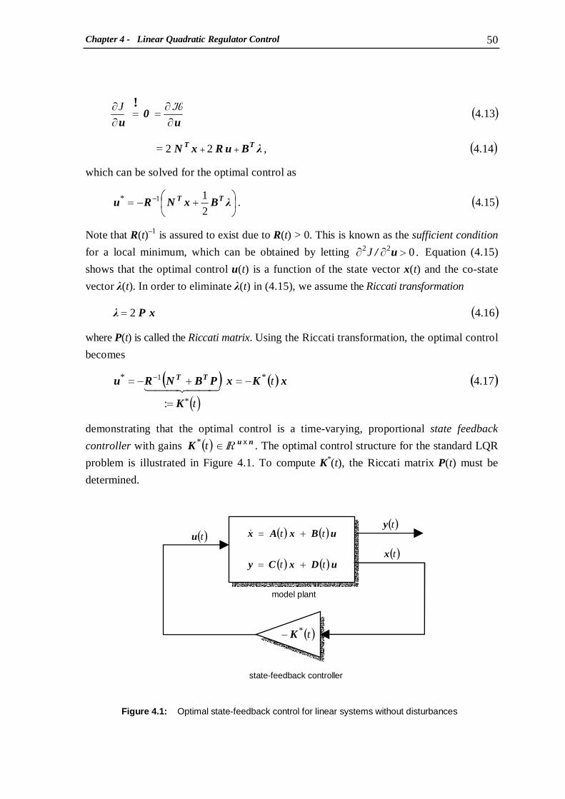
Chapter 4 - Linear Quadratic Regulator Control 50
which can be solved for the optimal control as
Note that R(t)–1 is assured to exist due to R(t) > 0. This is known as the sufficient condition
for a local minimum, which can be obtained by letting .022 J >∂∂ u/� Equation (4.15)
shows that the optimal control u(t) is a function of the state vector x(t) and the co-state
vector λ(t). In order to eliminate λ(t) in (4.15), we assume the Riccati transformation
where P(t) is called the Riccati matrix. Using the Riccati transformation, the optimal control
becomes
demonstrating that the optimal control is a time-varying, proportional state feedback
controller with gains ( ) nuK x t RI∈* . The optimal control structure for the standard LQR
problem is illustrated in Figure 4.1. To compute K*(t), the Riccati matrix P(t) must be
determined.
( )( )41.4,22
31.4
J
λBuRxN
u0
u
TT++=
∂∂==
∂∂ �!
( )51.4.2
11*
+−= − λBxNR u TT
( )61.42 xP λ =
( )( )
( ) ( )17.4
:
1* t
t
*
*
xKx
K
PBNR u TT −=
=
+−= −
44 344 21
Figure 4.1: Optimal state-feedback control for linear systems without disturbances
model plant
( )t*K−
state-feedback controller
( ) ( )( ) ( ) t t
t t
uDxCy
uBxAx
+=
+=&
( )ty
( )tx
( )tu
Chapter 4 - Linear Quadratic Regulator Control 51
( ) ( )23.4.0,lim t t
PPPP T ≥==∞→
4.1.3 Algebraic Riccati equation
Taking the derivative of the Riccati transformation (4.16) gives
Substitution of the Riccati transformation (4.16) in the Euler-Lagrange equation (4.12)
gives
Equating these two expressions for( )tλ& yields
With the state equations (4.1) and the control law (4.17) we find
This is valid for any state vector x(t) only if the following matrix equality holds:
Equation (4.22) is called the differential Riccati equation (DRE) and is a nonlinear first
order differential equation with a time-dependent solution P(t), Ramirez [61], Schwarz [71]
and Siouris [75]. For the infinite-time LQR problem Schwarz [71] proved that P(t)
approaches a constant matrix P, i.e.
Hence ( ) 0P =t& and Equation (4.22) becomes a time-dependent algebraic Riccati equation.
Since this equation does not depend on the state x(t) or control u(t), it can be computed
independently from the state differential equations which means that the optimal control
gain matrix K*(t) can be computed separately from the state dynamic response. In
practice, it will be pre-computed and stored for later use.
( )18.4.22 xPxP λ &&& +=
( )19.4.222 xPAuNxQλ T−−−=&
( )20.4. xPAuNxQxPxP T−−−=+ &&
( )( )[ ]{ } ( )[ ]
( )21.4
.11
xPAxPBNRNxQxPBNRBxAP
xPAuNxQuBxAPxP
TTTTT
T
++−+++−+=
++++=−
−−
&
( ) ( ) ( )22.4.1 QPBNRNBPPAAPP TTT +++−+=− − &
Chapter 4 - Linear Quadratic Regulator Control 52
For linear time-invariant (LTI) systems where A, B, C, D, Q, N and R are constant
matrices, the control task can be simplified. In this case, the unique solution P of the time-
invariant algebraic Riccati equation (ARE)
results in the optimal state-feedback controller with a constant state-feedback gain matrix
K * defined by (4.17):
The conditions for existence and uniqueness of the stabilizing optimal control
known as the Kalman criteria for controllability and observability, Ackermann [1],
Ramirez [61] and Schwarz [71], are as follows:
• the pair (A, B) is controllable, i.e.
• the pair ( ) TS
TS NBRAANNRQQ 11 :,: −−
−=−= is observable, i.e.
Within the MATLAB software, Shahian and Hassul [72], the LQR problem for
linear time-invariant systems can be solved for the objective functions defined by (4.2) and
(4.3) using the command ‘lqr‘ and ‘lqry’, respectively. Once the weighting matrices Q, N
and R in (4.2) or Qy and Ru in (4.3) are defined, the commands ‘lqr’ and ‘lqry’ will check
the conditions (4.26) and (4.27) automatically and return the Riccati matrix P and the
optimal state-feedback gain matrix K if those conditions are satisfied. The optimal control u
can then be derived easily by (4.17). The weighting matrices, therefore, can be considered
as the design parameters of the LQR problem.
( ) ( ) ( )24.4 1 0QPBNRNPBPAPA TTT =+++−+ −
( ) ( )25.4.1* PBNR K TT += −
[ ] ( )26.4,...,,, 1 n Rank =− B AABB n
( ) ( )27.4,...,,,1
n Rank =
−
QAQAQ TS
nTS
TS
TS
TS

Chapter 4 - Linear Quadratic Regulator Control 53
4.2 LQR for Linear Systems with Measurable Disturbances The standard LQR approach is used to synthesise an optimal controller for systems
without disturbances. In practice, however, most systems are influenced by exogenous
disturbances which also effect control optimality. In this section, the LQR problem for
linear systems excited by measurable disturbances will be presented. 4.2.1 Problem definition
Let us consider the linear time-varying system (3.77) including disturbances in a more
general form, i.e.
where ( ) ( ) wmw
wnw DB x x tt RIRI ∈∈ and . The vector of disturbances ( ) ww RI∈t is
assumed to be measurable in real time. The LQR problem for the system (4.28) is to find a
control input u(t) minimizing the objective function J defined by (4.3).
Substituting y(t) from (4.28) into (4.3) yields
( ) ( ) ( ) ( )( ) ( ) ( )
( )28.4
,0, 0
t t t
t t t
++=
=++=
wDuDxCy
xxwBuBxAx
w
w&
( ) ( )[ ]( ) ( ) ( )[ ][ ( )
( )( )
( )( )
( )]
{( ) ( ) ( )
}
( ) ( )[ ]( ) ( )29.4.,,,:
222
::
2
:
2
::
2
:
2
0
0
0
0
0
0
dt t
dt
dt
t
t
t
dt
t
t
t
dt
dt J
∫∫
∫
∫∫∫
∞
∞
∞
∞
∞
∞
=
+++++=
=
+
=
+
=
+
=
++
=
+
=
=
++++++=
+++++=
wxu
wRwuNwwNxuRuuNxxQx
w
R
DQDwu
N
DQDww
N
DQCx
u
R
RDQDuu
N
DQCxx
Q
CQCx
uRuwDQDwwDQuDxCuDxCQuDxC
uRuwDuDxCQwDuDxC
wT
wuT
wxTTTT
w
wyTw
T
wu
yTw
T
wx
wyTT
uyTT
yTT
yTT
uT
wyTw
Twy
Ty
T
uT
wyT
w
��
434214342143421
44 344 214342143421

Chapter 4 - Linear Quadratic Regulator Control 54
Different from the standard LQR problem is the second group of terms depending on the
disturbances w(t). Therefore, the control law has to be a function of both x(t) and w(t). It
should be noted that the solution of the optimal control problem for disturbed linear
systems via the LQR approach requires both the state x(t) and disturbance w(t) to be
known or measurable over the entire time domain.
4.2.2 Solution based on the Pontryagin’s maximum principle
The Hamiltonian for the optimal control problem of linear systems (4.28) with
measurable disturbances can be defined as
Based on the Pontryagin’s maximum principle, the necessary condition for a local
minimum is given by the Euler-Lagrange equation
and the optimal control equation
The optimal control can be derived from (4.32) as
In order to eliminate the co-state vector λ(t) from Equation (4.33), the Riccati
transformation is assumed as
( ) ( ) ( )( ) ( )
( ) ( )30.4.
222
,,,:,,,,
tt
wBuBxAλ
wRwuNwwNxuRuuNxxQx
wBuBxAλwxuλwxu
wT
wT
wuT
wxTTTT
wT
+++
+++++=
+++=��
( ) ( )31.4222 λAwNNuQxx
λ Txw +++−=
∂∂−= �
&
( )33.4.2
11*
++−= − λBwNxNRu TTuw
T
( ) ( )34.42 ξxPλ −=
( )32.4.222 λBwNRuxNu
0 TTuw
T +++=∂∂= �
Chapter 4 - Linear Quadratic Regulator Control 55
where P(t) = PT(t) and ξ(t) are the so-called Riccati matrix and Riccati vector, respectively.
Then the optimal control becomes
This equation shows that the optimal control ( )*tu for the stated problem includes not only
state-feedback control ( )t *xu , but also disturbance feed-forward control ( )t *
wu . To
complete the optimal control ( )*tu , the Riccati matrix P(t) and Riccati vector ξ(t) must be
defined.
Taking the derivative of the Riccati transformation (4.34) gives
Substituting the Riccati transformation (4.34) in the Euler-Lagrange equation (4.31) yields
Equating these two expressions for( )tλ& yields
The state equations (4.28) yield
or after rearranging
With the control law (4.35), the equation becomes
( )( )[ ]
( )( )[ ]
( )( )35.4.
:: **
*
11
1
t
t
444 3444 21444 3444 21
w
TTuw
x
TT
TTTuw
T
u
ξBwNR
u
xPBNR
ξBxPBwNxNRu
=
−−+
=
+−=
−++−=
−−
−
( ) ( ) ( )[ ] .0 wPBNξAξuPBNxQxPAxPAxP wxwTT =+−+−+++++ &&
( )[ ] ( )38.4.
ξxPAwNuNxQξxPxP Txw −+++−=−+ &&&
( ) ( ) ( )[ ]( ) ( )[ ] ( )[ ]
or
1
1
0wPBNξAξξBwNRPBN
xPBNRPBNxQxPAxPAxP
wxwTTT
uw
TTT
=+−+−−−++
+−+++++
−
−
&
&
( ) ( )36.4.2 ξxPxPλ &&&& −+=
( )[ ] ( )37.4.2 ξxPAwNuNxQλ Txw −+++−=&
( ) ( )[ ]
ξxPAwNuNxQξwBBuAxPxP Txww −+++−=−+++ &&
Chapter 4 - Linear Quadratic Regulator Control 56
Equation (4.39) is satisfied for any vector of states x(t) and disturbances w(t) only if the
two lines vanish separately. This results in the already known differential Riccati matrix
equation (4.22), i.e.
and the so-called differential Riccati vector equation
Let ( )t*xK denote the optimal state-feedback controller where according to Equation (4.35)
the differential Riccati vector equation (4.41) can be simplified to
For the infinite-time problem we get ( ) ( ) 0ξ0P == t t && and , see Ramirez [61] and Schwarz [71].
Equations (4.40) and (4.43) then become the time-varying algebraic equations resulting in
the time-dependent Riccati matrix P(t) and vector ξ(t), respectively. In this case the
Riccati vector ξ(t) can be computed by
With the state-feedback controller ( )t*xK and the Riccati vector ξ(t) defined by (4.42) and
(4.44), respectively, the disturbance feed-forward control ( )t*wu in (4.35) can be written as
( )[ ] ( ) ( )[ ]( )41.4
.11
0 wPBNNRPBNξBRPBNAξ wxwTuw
TT =+−+++++ −−&
( ) ( )43.4.** 0 wPBNNKξBKAξ wxwTuw
T
xTT
xT
=
+−+
++&
[ ( ) ] ( )[ ( ) ]{ }( ) ( )45.4: *
*** 11
t
w
K
PBNNKBKABNRu
wuw
wxwTuw
T
xTT
xTTT
uww444444444444 3444444444444 21
xRI∈=
+−++−=−
−
( ) ( ) ( )42.4,, ** 1 t nux
TT
xKPBNRK xRI∈+−= −
( ) ( ) ( )
40.4,1 0 QPBNRNBPPAAPP TTT =+++−++ −&
( ) ( )[ ]( )[ ] ( ) ( )[ ]
( )39.4
.11
1
0 wPBNNRPBNξBRPBNAξ
xQPBNRPBNPAPAP
wxwTuw
TT
TTT
=+−+−++−−
+++−++
−−
−
&
&
( ) ( )44.4.**1
wPBNNKBKAξ wxwTuw
T
xTT
xT
+−
+−=−

Chapter 4 - Linear Quadratic Regulator Control 57
where ( )t*wK represents the optimal disturbance-feed forward controller. Consequently,
the optimal control is defined by
For the case of linear time-invariant (LTI) systems, P(t) = P is a constant matrix
which is the unique solution of the algebraic Riccati equation (4.24) resulting in the
constant optimal gain matrices *xK and *wK .
Figure 4.2 shows the optimal control structure for linear systems with measurable
disturbances. It can be realized clearly that the standard LQR problem described in
Section 4.1 is a special case of the stated problem with w(t) = 0.
Figure 4.2: Optimal control structure for linear systems with measurable disturbances
( )46.4.***** wKxKuuu wxwx −−=+=
model plant
state-feedback controller
+
disturbance-feed forward controller
( )ty
( )tw ( )twu
( )txu
( )tx( )tu
( ) ( ) ( )( ) ( ) ( )wDuDxCy
wBuBxAx
w
w
t t t
t t t
++=
++=&
( )t*wK−
( )t*xK−

Chapter 4 - Linear Quadratic Regulator Control 58
4.3 Application of LQR Control to the Spatial Car Model
The linear time-invariant spatial car model (3.78) results from constant velocity v and
track curvature κ is used as an example to design the optimal control based on LQR
approach. Since the lateral acceleration ay as disturbance of the system can be measured
online by an acceleration sensor, the solution of the LQR problem for linear systems with
measurable disturbances introduced in the above section can be applied. To estimate the
dynamic characteristics of vehicles in yaw motion, automotive performance criteria
specified for the spatial car model are introduced. Advantages and drawbacks of the LQR
control design applied to the spatial car model with active suspensions will be shown.
4.3.1 Dynamic criteria for the spatial car model
During cornering, the vehicle weight is transferred between the wheels resulting in load
changes. Vehicle ride safety and road handling characteristics, however, are determined
by the dynamic wheel loads. High loads allow greater longitudinal and lateral
transmission forces between wheels and ground. On the contrary, low wheel loads can
cause loss of controllability of the car. Larger magnitudes of the roll and pitch angles will
indirectly influence ride safety as contact force magnitudes might reach zero causing lift-
off, Sampson [67]. The most commonly used criterion for ride safety of passenger cars is
the integral function of quadratic dynamic wheel loads, Mitschke [50], Popp and
Schiehlen [59]. Since the dynamic wheel loads are proportional to the suspension
deflections, the integral of quadratic suspension deflections can be used as a substitutive
criterion, Bestle [7].
For the spatial car model, the four wheels of the car are assumed to be mass-less
points which keep their traces on the plane track surface. The dynamic wheel loads are,
therefore, proportional to the vertical displacements of the suspension nodes zSi, i = 1(1)4,
and thus can be used to represent the ride safety criterion, Ammon [2]:
( ) ( )4.47 .
4
10
4
1
21 dt tz
T f
∫ ∑=
=T
iSi
Chapter 4 - Linear Quadratic Regulator Control 59
Ride comfort is mainly characterized by the accelerations of the driver and
passengers, Mitschke [50], Popp and Schiehlen [59]. For simple models, the accelerations
of the car body can be used alternatively to estimate vehicle ride comfort. While the
vertical acceleration is of special interest for cars riding on uneven roads, the roll
acceleration of the car body must be taken into consideration for cars in yaw motion on
even roads. The ride comfort criterion for the spatial car model can then be defined by
For passenger cars using active suspensions, improving ride safety and ride comfort
often requires a large expense of control energy. Control effort, therefore, must be
considered as an objective to be minimized for passenger cars using active suspensions.
The control effort criterion for the spatial car model can be expressed by
The formulas (4.47) − (4.49) represent root-mean-squares (RMS/r.m.s) of suspension
displacements, car body roll acceleration and control forces, respectively. It should be
noted that minimizing the integrals in (4.47) − (4.49) will minimize f1, f2 and f3,
respectively. These integrals, therefore, can be also treated as corresponding criteria and
will be used alternatively to define the objective function for LQR control design.
4.3.2 Spatial car model simulation
As illustrated in Figure 4.3, the car may move along a circular track of radius R = 10 [m]
with constant velocity v = 30 km/h ≈ 8.33 m/s. At the starting point, the lateral
acceleration of the car jumps to a constant value ay = v2/R ≈ 6.94 m/s2 as a step function
exciting the system. The car parameters are given in Appendix A.
( ) ( )4.48 . 1
0
22 dt t
T f
∫=T β&&
( ) ( )4.49 .4
10
4
1
23 dt tu
T f
∫ ∑=
=T
ii

Chapter 4 - Linear Quadratic Regulator Control 60
4.3.3 LQR design for the spatial car model
In order to apply the LQR control to the spatial car model, the objective function must be
determined first. The quadratic objective function for the spatial car model can be defined
as weighted sum of the integrals in (4.47) − (4.49)
( )50.4.0
4
1
23
0
22
0
4
1
21 dt u w dt w dt z w J
∫∑∫∫∑ ∞
=
∞∞
=
++=i
ii
Si β&&
Figure 4.3: Simulation of the spatial car model in cornering
yI
xI
v = 8.33 [m/s]
R = 10 [m]
ay = 6.94 [m/s2]

Chapter 4 - Linear Quadratic Regulator Control 61
With the vectors of control inputs u and measured outputs y defined by (3.64) and (3.75),
respectively, the objective function (4.50) can be expressed in the regular form of the LQR
problem (4.3) by introducing the weighting matrices
where w1, w2 and w3 are the weighting factors on ride safety, ride comfort and control
effort, respectively. Once the weighting matrices Qy and Ru are determined, the MATLAB
function ‘lqry’ will give the Riccati matrix P and the optimal state-feedback control
gain *xK . The optimal disturbance-feed forward control gain*wK can be then easily derived
from (4.45) with the matrices xwTuw NNR and , defined in Equation (4.29). By choosing
proper weighting factors, desired solutions can be obtained.
{ }
{ } ( )51.4,,,
and
,,,,
3333
21111
w w w w diag
w w w w w diag
=
=
u
y
R
Q
0 0.5 1 1.5 2 2.5-600
-400
-200
0
200Control Force at Front-Left Wheel
time t[s]
u 1 [
N]
0 0.5 1 1.5 2 2.5-200
-100
0
100
200Roll Acceleration
β [de
g/s2
]
0 0.5 1 1.5 2 2.50
1
2
3Suspension Displacement at Front-Left Wheel
zs1 [
cm]
w1=0 , w
2=0 , w
3=10-2
w1=2x10⁷, w
2=0 , w
3=10-2
w1=0 , w
2=2x10³, w
3=10-2
w1=2x10⁷, w
2=2x10³, w
3=10-2
..
Figure 4.4: Simulation results obtained from LQR design

Chapter 4 - Linear Quadratic Regulator Control 62
Figure 4.4 shows the simulation results corresponding to different values of the
weighting factors. During simulation the system takes on the form of the linear-time
invariant system with constant disturbance w = ay (3.78). The resulting optimal control
gains 64* x RI∈xK and 14* xRI∈wK are given in Table 4.1. For clearance, only the time
response of the vertical displacement of the suspension node zS1 and the control force u1 at
the front-left wheel are plotted in the figure. In case 1 denoted by the dotted lines, only the
control effort criterion is minimized resulting in*xK , *
wK = 0 which means that no control
energy is provided by the actuators. The dash-dotted and dashed lines corresponding to
case 2 and case 3 represent the responses of the system when the ride safety and ride
comfort criterion are optimized separately, respectively. In the last case described by the
solid lines all three criteria are penalized and a compromise solution is derived.
weighting factors optimal control gains
case
w1 w2 w3 *xK (x 104 ) *
wK
1 0 0 10–2
0 0
2
2x10⁷
0
10–2
3
0
2x10³
10–2
4
2x10⁷
2x10³
10–2
Table 4.1: Optimal state-feedback gain matrix *xK and disturbance-feed forward gain vector *
wK corresponding to different weighting factors
0.4622 0.1496- 0.2681 5.6352 1.1892- 3.0555
0.4597 0.1484 8 0.2685.3511 1.3990 3.0438
0.3883- 0.1496- 0.4084 2.7736- 1.3957- 2.9099
0.3908- 0.1508 0.4091 3.0599- 1.2132 2.8980
0.0150- 0.0821- 0.0009- 0.0393- 1.0185 0.0008-
0.0171 0.0872 0.0009 0.0395 1.1814- 0.0007-
0.0169- 0.0850- 0.0008- 0.0379- 1.1796 0.0006
0.0155 0.0856 0.0010 0.0415 1.0378- 0.0007
0.4478 0.1654- 0.2679 5.5398 0.2636 3.0501
0.4750 0.1634 0.2690 5.4497 0.1685- 3.0487
0.4036- 0.1640- 0.4082 2.8718- 0.1732 2.9049
0.3761- 0.1674 0.4094 2.9627- 0.2623- 2.9035
45.1908-
70.7979
74.7698-
42.1406
39.3411-
41.6755
41.8481-
39.8123
46.3534-
51.0035
52.2497-
45.8808
Chapter 4 - Linear Quadratic Regulator Control 63
The simulation results show the effectiveness of active suspension systems with LQR
control on ride safety and ride comfort of the car in cornering and the usefulness of the LQR
design as the optimal gain matrices with a large number of components can be easily
obtained by choosing appropriate weighting factors. However, if the control problem is
subject to constraints on the states, measured outputs or control inputs, the optimal solutions
may not be found by choosing the weighting factors by hand.
In order to overcome the drawbacks of the LQR approach in the optimal controller
design problem, multi-criterion optimization must be applied. The combination of multi-
criterion optimization methods and the LQR algorithm for defining the optimal controllers
for the spatial car model will be introduced in the next chapter.

Chapter 5 - Multi-criterion Optimization 64
Chapter 5
Multi-criterion Optimization
In technical applications, multiple goals have to be taken into account which often are in
conflict. Multi-criterion optimization (MCO) is a powerful tool for finding the best
compromise solution balancing the conflicts, and therefore is of great importance in
practice, particularly in engineering design. In this chapter, two effective MCO methods
for generating the trade-off solutions, namely the compromise method and the recursive
knee approach, will be introduced. MCO problems will be defined for both the passive
and active suspension case. An optimization method combining the MCO and LQR
algorithm in order to reduce the number of design variables will be presented. Significant
improvements in ride safety and ride comfort for the passive and active suspension also
will show the effectiveness of the approach.
5.1 Overview on Multi-criterion Optimization
Multi-criterion optimization (MCO) or vector optimization refers to the process of
optimizing simultaneously a collection of objective functions. The general multi-criterion
optimization problem is to find a vector of design variables ,, hpp RI∈ optimizing the
vector of criteria ( ) ,:, nhfpf RIRI → subject to equality constraints g(p) = 0, inequality
constraints h(p) ≤ 0 and variable bounds pl and pu:
( )
{ ( ) ( ) } ( )1.5:,:,,,:
where
mhlhulh hgppp0ph0pgp
pfp
RIRIRIRIRI →→≤≤≤=∈=
∈
opt
P
P

Chapter 5 - Multi-criterion Optimization 65
is the set of admissible designs or feasible design space, and opt means minimization of
all individual criteria fi(p), i = 1(1)n. The criteria define a transformation of the feasible
design space P to the attainable criterion space F ,
Figure 5.1 illustrates the mapping of the feasible design space P to the attainable criterion
space F for a bi-criterion case.
If we have only one single objective, i.e. n = 1, the problem is a scalar optimization
problem where the scalar objective defines a total order on P . This means all design
points P∈p are comparable to each other. In this case, a design point p* is called a global
minimum if
and called a local minimum, if there exits an open set 2RI⊂U around p* such that
( ){ } ( )2.5.: PF ∈∈= ppf nRI
Figure 5.1: Mapping from design space 2RI⊂P into criteria space 2RI⊂F
( ) ( ) ( )3.5,* ff P∈∀≤ ppp
( ) ( ) ( )4.5.* ff �PU ∩∈∀≤ ppp
P
p2
p1
f2
f1
F
p f(p)
design spacehRI criterion space
nRI
f
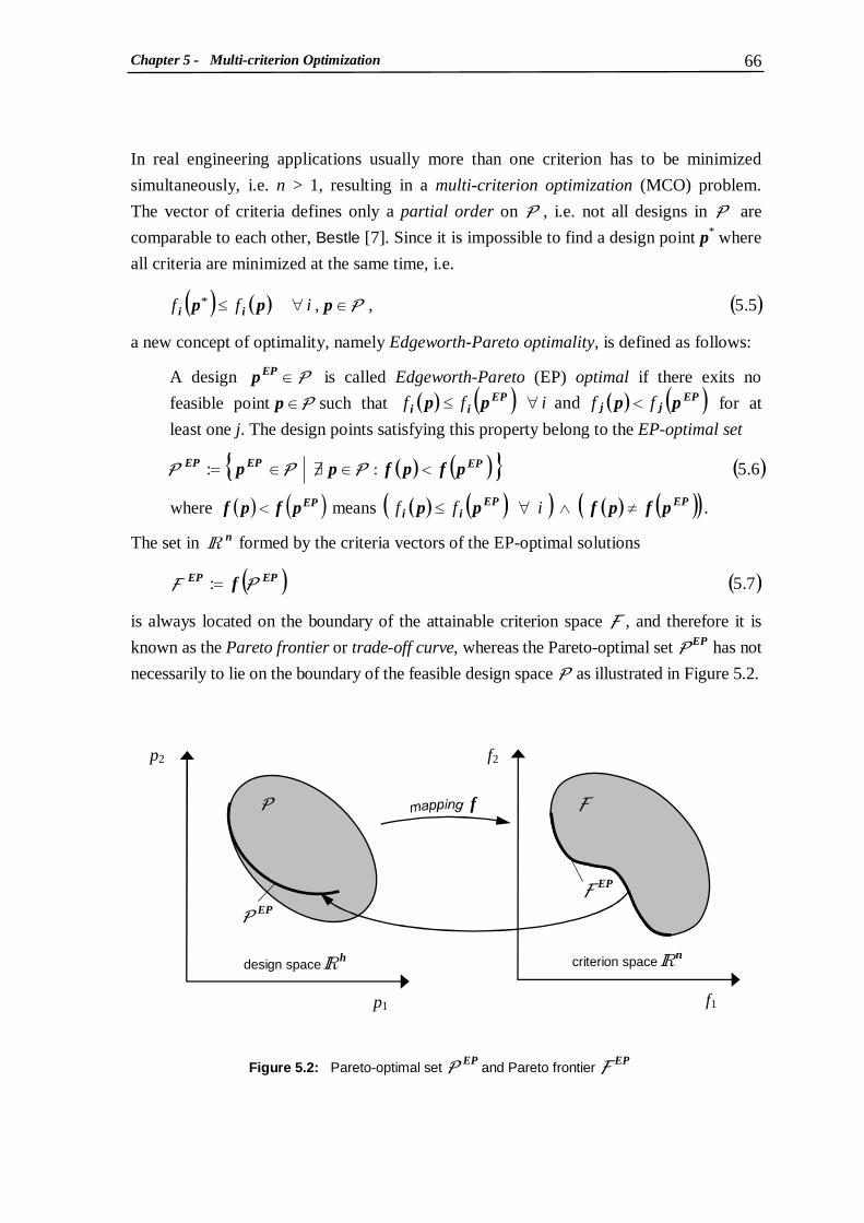
Chapter 5 - Multi-criterion Optimization 66
In real engineering applications usually more than one criterion has to be minimized
simultaneously, i.e. n > 1, resulting in a multi-criterion optimization (MCO) problem.
The vector of criteria defines only a partial order on P , i.e. not all designs in P are
comparable to each other, Bestle [7]. Since it is impossible to find a design point p* where
all criteria are minimized at the same time, i.e.
a new concept of optimality, namely Edgeworth-Pareto optimality, is defined as follows:
A design P∈EPp is called Edgeworth-Pareto (EP) optimal if there exits no
feasible point P∈p such that ( ) ( ) ( ) ( )EPjj
EPii pppp ff i ff <∀≤ and for at
least one j. The design points satisfying this property belong to the EP-optimal set
where ( ) ( )EPpfpf < means ( ) ( )( ) ( ) ( )( )EPEPii pfpfpp ≠∧∀≤ i ff .
The set in nRI formed by the criteria vectors of the EP-optimal solutions
is always located on the boundary of the attainable criterion space F , and therefore it is
known as the Pareto frontier or trade-off curve, whereas the Pareto-optimal set P EP has not
necessarily to lie on the boundary of the feasible design space P as illustrated in Figure 5.2.
( ) ( ) ( )5.5,,* i ff �P∈∀≤ ppp ii
( ) ( ){ } ( )6.5: : / EPEPEP pfpfpp <∈∃∈= P PP
( ) ( )7.5: EPEP f PF =
Figure 5.2: Pareto-optimal set P EP and Pareto frontier F EP
P
p2
p1
f2
f1
F
design spacehRI criterion space
nRI
f
P EP
F EP

Chapter 5 - Multi-criterion Optimization 67
Figure 5.3: Individual minima F1* and F2
* and CHIM
The end points Fi*of the Pareto frontier are called individual minima. They are defined
by vectors fi*:= [ f1(pi
*), …, fi *, …, fn(pi
*)]T where pi* denotes the individual optimizer of
the criterion fi(p) with minimum fi *, i.e.
The hyper-plane running through all individual minima is known as the convex hull of the
individual minima (CHIM), Das and Denis [19]. For the bi-criterion problem, the CHIM
is the line joining the individual minima F1* and F2
* , which are respectively defined by
vectors:
see Figure 5.3.
f2
f1
F
f1*
f2*
F2*
F1*
CHIM
f21*
f12*
f1*
f2*
( ) ( ) ( )8.5.11,min: n i f
f * =∈
= pp
iiP
( )( )
( )( ) ,:,:
2
21
22
21
21
2
1
12
11
1**
f
f
f
f
f
f
f
f
*
*
*
*
*
*
*
*
=
=
=
=
p
pf
p
pf

Chapter 5 - Multi-criterion Optimization 68
Figure 5.4: Compromise method for the bi-criterion problem with r = 2
5.2 Multi-criterion Optimization Methods
In general, EP-optimal solutions are not unique, thus the designer has to choose a single EP-
optimal point from the set P EP as the desired solution instead. To find such points or a
representative subset of P EP, the multi-criterion optimization problem usually has to be
reduced to scalar utility problems. In this section, two scalarization approaches applied to the
MCO problem for the spatial car model for obtaining a sample set of points of the Pareto
frontier, namely the compromise method and the recursive knee approach, are introduced.
Other MCO methods can be found in Bestle [7], Collette and Siarry [16] and Deb [20].
5.2.1 Compromise method
The compromise method entails minimization of one of the criteria fr(p), while expressing
the remaining criteria in the form of inequality constraints:
In the above formulation, εi represents an upper bound for fi and can be considered as
scalarizing parameter, Das [17, 18]. By progressively changing the constraint values εi,
different points on the Pareto frontier can be sampled.
( ) ( ) { }{ } ( )9.5.\,: min r i εf wheref nI PP
P
∈≤∈=∈
iir
rr
pppp
f2
f1 f1*
F 1*
ε1
F EP
f12*
F 2*
f2*
f21*
): (PF f=
f (p*)
f (P 2)

Chapter 5 - Multi-criterion Optimization 69
Figure 5.4 visualizes the working of the compromise method for a bi-criterion case,
where f2 is retained as a criterion, while f1 is treated as a constraint f1 ≤ ε1. With this
constraint, the original attainable criterion space F is reduced to F 2 := f (P 2), which is the
left-upper portion of F bounded by ε1. The solution of the problem (5.9) depends strongly
on the value of the constraint ε1. As can be seen from the figure, if ε1 < f1*:= f1(p1
*) is
chosen, there exits no feasible solution to the stated problem. On the other hand, if
ε1 > f12*:= f1(p2
*) is used, the entire search space is feasible and the resulting problem finds
the solution point F2*.
A remarkable advantage of the compromise method is that the EP-optimal solutions
can be found even if the criterion space is non-convex. Moreover, these solutions can be
distributed evenly on the Pareto frontier by changing appropriately the values for εi within
the minimum and maximum value of the individual criterion fi. For the bi-criterion case as
illustrated in Figure 5.4, N EP-optimal points on the Pareto frontier F EP between the
individual minima F1* and F2
* can be found by choosing the constraint values of ε1 as
This formulation means that ε1 is reduced evenly from f12* to f1
* with the constant
difference ∆ε1.
The effectiveness of the compromise method is, however, limited to problems with
not more than two criteria. For problems with more than two criteria, values of the
constraints for more than one criterion have to be determined in advance. Many sets of the
constraint values need to be chosen and the corresponding number of associated
optimization problems increases. This results in wasted computational resources as will
be shown in Section 5.4, where the compromise method is applied to the three-criterion
optimization problem defined for the spatial car model.
( ) ( )
( ) ( ).:,:,1
:
where
10.511,
**21
21111
12
11
12
11
f f f f N
ff ε
N k ε k fε
***
*
*
pp
k
==+−=∆
=∆−=

Chapter 5 - Multi-criterion Optimization 70
5.2.2 Recursive knee approach
The recursive knee approach is a technique based on the normal-boundary intersection
(NBI) method introduced first by Das and Denis [19]. This technique was then modified
and programmed by Wachal and Bestle [86], whose main idea is presented below.
The NBI sub-problem maximizes the distance along a normal while staying feasible
in an attempt to find the point of intersection between the normal and the Pareto frontier.
Let F be the matrix defined as F := [ f1*, f2
*, …, fn* ]. Then an arbitrary point A on the
CHIM can be determined by vector rA := Fa, where na RI⊂∈A is treated as scalarizing
parameter with
At a given point A, define a vector n normal to the CHIM pointing away from the origin.
Then, the NBI sub-problem for obtaining a single EP-optimal solution can be formulated
as follows
The NBI algorithm for a bi-criterion case is illustrated in Figure 5.5. For finding a
representative subset of solutions, point A has to be moved along the CHIM, and thus the
value of vector a has to be varied. A systematic method of setting a in order to generate
an evenly distributed set of EP-optimal points on the Pareto frontier can be found in Das
and Denis [19].
If the origin point of the line Fa + tn, i.e. point A, is allowed to be an optimization
variable itself, the solution to the problem yields the EP-solution that is furthest from the
CHIM in normal direction. The NBI sub-problem (5.12) therefore has to be reformulated
with a becoming a design variable as well:
( )11.5.0,1:1
a a
≥=∈= ∑
=i
n
ii
na RIA
( )( )12.5.
,
,
min
t
to subject
t
t
A
P
∈
=+
∈
a
pfnaF
p

Chapter 5 - Multi-criterion Optimization 71
Figure 5.5: Normal-boundary intersection (NBI) method
This sub-problem is called the knee sub-problem, and the solution to this sub-problem
characterizes the knee of the Pareto frontier.
Once the knee of the Pareto frontier is obtained, the CHIM can be refined by
considering the piece-wise linear approximation joining the individual minima with the
knee, as shown in Figure 5.6. Each linear segment can be considered as a separate sub-
CHIM, and the knee sub-problem can be solved for each sub-CHIM. The process can be
repeated recursively to generate several points on the Pareto frontier.
( )( )13.5.
,
,,
min
t
to subject
t t
A
P
∈
=+
∈
a
pfnaF
ap
f1
f1*
n
.
rA = Fa
f(p*)
tn
F2*
F1*
f2*
F
f2
A F
EP
CHIM
|minAt|

Chapter 5 - Multi-criterion Optimization 72
Figure 5.6: Recursive knee approach
Since the solution to the knee sub-problem yields the point that is ‘the furthest’ from
the piece-wise linear approximation, every solution to a subsequent knee sub-problem
yields the best refinement of the approximation possible. This procedure results in
building a good approximation to the Pareto frontier by solving a minimal number of
computationally intensive sub-problems.
Since the origin point of the normal direction is a variable in the knee sub-problem,
the disconnected nature of the Pareto frontier poses no infeasibility problem for the
technique as it did for the traditional NBI method. The recursive knee approach can easily
be applied to problems with more than two criteria as well. Since the approach finds the
EP-solutions that would best improve the piece-wise linear approximation, it does not
miss important parts of the Pareto frontier, Das [18].
The pre-eminence of the recursive knee approach over the compromise method to the
three-criterion optimization problem of the spatial car model will be shown in Section 5.5.
f1
F2*
F1*
f2
K
F
|tmin|
Chapter 5 - Multi-criterion Optimization 73
5.3 MCO Problem for Passive Suspension
In this section, a bi-criterion optimization problem for the spatial car model with a passive
suspension system will be defined and solved with the compromise method. The
significant improvements in both car ride safety and ride comfort will be shown.
5.3.1 Problem definition
For the case of a passive suspension, the two objectives to be minimized are ride safety
(4.47) and ride comfort (4.48). The chosen design parameters are the damping coefficients
bf and br of the front and rear suspensions, the stiffnesses kf and kr of the front and rear
suspensions, and the modified rotational stiffnesses rf and rr of the front and rear anti-roll
bars. The MCO problem for the spatial car model with a passive suspension then reads as
5.3.2 Optimization results based on the compromise method
To apply the compromise method, the comfort criterion f2 is chosen to be minimized,
while the ride safety criterion f1 is expressed as inequality constraint. The MCO problem
for the passive suspension case (5.14) then reduces to
( ) ( ){ } ( )15.5.: min 112
22
εf wheref ≤∈=∈
pppp
PP
P
( ) ( ) [ ][ ]{ }
[ ][ ] ( )14.5.15000,25000,25000,25000,2000,2000
,5000,15000,15000,15000,1000,1000
,,,,,:
,,:,min
6
21
where
r r k k b b
f f
Tu
Tl
ulTrfrfrf
T
p
p
pppp
pfpfp
=
=
≤≤∈==
=∈
����������������
����������������
����
����������������
���������
RIP
P
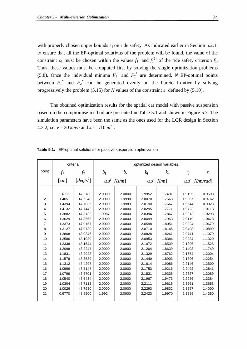
Chapter 5 - Multi-criterion Optimization 74
with properly chosen upper bounds ε1 on ride safety. As indicated earlier in Section 5.2.1,
to ensure that all the EP-optimal solutions of the problem will be found, the value of the
constraint ε1 must be chosen within the values f1* and f1
2* of the ride safety criterion f1.
Thus, these values must be computed first by solving the single optimization problems
(5.8). Once the individual minima F1* and F2
* are determined, N EP-optimal points
between F1* and F2
* can be generated evenly on the Pareto frontier by solving
progressively the problem (5.15) for N values of the constraint ε1 defined by (5.10).
The obtained optimization results for the spatial car model with passive suspension
based on the compromise method are presented in Table 5.1 and shown in Figure 5.7. The
simulation parameters have been the same as the ones used for the LQR design in Section
4.3.2, i.e. v = 30 km/h and κ = 1/10 m−1.
criteria optimized design variables
bf br kf kr rf rr
point f1
[cm]
f2
[deg/s2] x103 [Ns/m] x104 [N/m] x104 [N/m/rad]
1 2 3 4 5 6 7 8 9
10 11 12 13 14 15 16 17 18 19 20 21
1.4905 1.4651 1.4394 1.4132 1.3882 1.3629 1.3373 1.3127 1.2868 1.2586 1.2338 1.2098 1.1831 1.1578 1.1312 1.0999 1.0799 1.0540 1.0304 1.0026 0.9770
47.5780 47.6340 47.7035 47.7442 47.8133 47.8568 47.9157 47.9730 48.0346 48.1030 48.1644 48.2247 48.2928 48.3589 48.4297 48.5147 48.5701 48.6434 48.7113 48.7930 48.9500
2.0000 2.0000 2.0000 2.0000 1.9987 2.0000 2.0000 2.0000 2.0000 2.0000 2.0000 2.0000 2.0000 2.0000 2.0000 2.0000 2.0000 2.0000 2.0000 2.0000 1.9924
2.0000 1.9998 1.9983 2.0000 2.0000 2.0000 2.0000 2.0000 2.0000 2.0000 2.0000 2.0000 2.0000 2.0000 2.0000 2.0000 2.0000 2.0000 2.0000 2.0000 2.0000
1.9952 2.0070 2.0190 2.0295 2.0394 2.0499 2.0598 2.0710 2.0828 2.0953 2.1072 2.1204 2.1329 2.1440 2.1614 2.1753 2.1831 2.1967 2.2111 2.2293 2.2423
1.7491 1.7563 1.7667 1.7771 1.7867 1.7953 1.8051 1.8145 1.8261 1.8384 1.8509 1.8639 1.8762 1.8903 1.9086 1.9216 1.9338 1.9473 1.9615 1.9832 1.9970
1.9195 1.9367 1.9544 1.9723 1.9913 2.0119 2.0324 2.0498 2.0741 2.0984 2.1206 2.1403 2.1654 2.1896 2.2146 2.2492 2.2687 2.2986 2.3261 2.3557 2.3889
0.9593 0.9762 0.9928 1.0118 1.0298 1.0478 1.0679 1.0899 1.1079 1.1320 1.1528 1.1749 1.2004 1.2254 1.2500 1.2841 1.3089 1.3384 1.3653 1.4000 1.4350
Table 5.1: EP-optimal solutions for passive suspension optimization
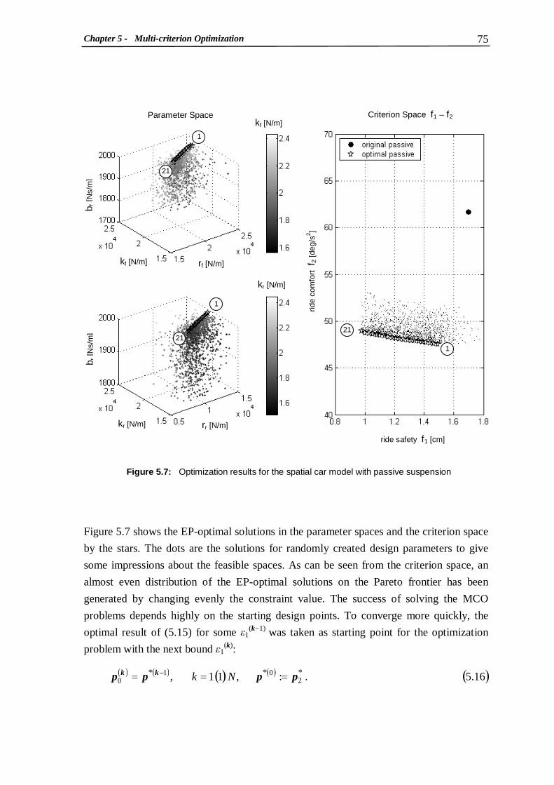
Chapter 5 - Multi-criterion Optimization 75
Figure 5.7 shows the EP-optimal solutions in the parameter spaces and the criterion space
by the stars. The dots are the solutions for randomly created design parameters to give
some impressions about the feasible spaces. As can be seen from the criterion space, an
almost even distribution of the EP-optimal solutions on the Pareto frontier has been
generated by changing evenly the constraint value. The success of solving the MCO
problems depends highly on the starting design points. To converge more quickly, the
optimal result of (5.15) for some ε1(k−1) was taken as starting point for the optimization
problem with the next bound ε1(k):
Figure 5.7: Optimization results for the spatial car model with passive suspension
( ) ( ) ( ) ( ) ( )16.5.:,11, ***2
010 N k pppp kk
===−
kf [N/m]
kr [N/m]
rf [N/m]
rr [N/m]
kr [N/m]
kf [N/m]
b f [N
s/m
] b r
[Ns/
m]
ride safety f1 [cm]
ride
com
fort
f2
[deg
/s2 ]
Parameter Space Criterion Space f1 – f2
1
21
21 21
1
1

Chapter 5 - Multi-criterion Optimization 76
Compared to the case of the original passive suspension with parameters given in
Appendix A denoted by the black circle in Figure 5.7, the optimized passive suspension
improves the car ride safety by about 12% − 42% and ride comfort by 21% − 23%. The
obtained results show that improving ride safety in cornering situations requires an increase
in both the springs and anti-roll bars stiffness, which is contrary to the case improving ride
comfort.
5.4 MCO Problem for Active Suspension
Ride safety and ride comfort of the car can be further improved by using active
suspension. In this section, the three-criterion optimization problem for the spatial car
model with active suspension will be defined. An optimization method combining the
multi-criterion optimization concept with the linear quadratic regulator (LQR) algorithm
will be introduced. The drawback of the compromise method compared to the recursive
knee approach for the three-criterion optimization problem will be exposed based on the
results obtained from the proposed optimization algorithm.
5.4.1 Problem definition
Different from the passive suspension case, the existence of the control forces generated
by actuators in the active suspension system requires control effort which has to be taken
into account in an optimization problem. The criteria vector, therefore, includes not only
ride safety f1 and ride comfort f2, but also the control effort criterion (4.49). The spatial
car model is set up the same way as in the case of LQR design and the control structure
with state-feedback and disturbance-feed forward controller is according to Figure 4.2.
The parameters of the optimized passive suspension corresponding to the 10th row in
Table 5.1 are used as constants for the passive suspension parts. The design variables are
the components kxij of the 4x6-state-feedback gain matrix Kx, and the elements kwj of the
4x1-disturbance-feed forward gain vector Kw. The MCO problem for the spatial car model
with active suspension can then be stated as

Chapter 5 - Multi-criterion Optimization 77
In the above formulation, the design parameters are considered as unbounded. However,
an inequality constraint h(p) is used to limit the control forces, according to the limited
capability of real actuators.
5.4.2 MCO with LQR control
Solving the MCO problems of the form (5.17) directly for the optimal control gains *xK
and *wK without pre-knowledge about the solutions or bounds would be rather time-
consuming, especially for large systems like the spatial car model. This problem can be
solved faster by applying the LQR algorithm. Instead of finding directly the components
of the controllers via optimization, the LQR algorithm is used to compute *xK and *wK
with weighting factors w1, w2 and w3 provided by the optimizer.
With inclusion of LQR control, the MCO problem (5.17) can be reformulated as
follows:
( ) ( ) [ ][ ] ( ){ }
( ) ( ) ( )17.5.500maxmax:
0...,,,...,,:
,,,,min
28414611
321
tu
h
where
h k
k
k
k
f f f
−
=
≤∈==
=∈
iti
Twwxx
T
p
pp
pfpfp
RIP
P
( ) ( ) [ ]
[ ] ( ){ }[ ][ ]
( ) ( ) ( )18.5.500maxmax:
,10,10,10
,10,0,0
0,,,:
,,,,min
288
6
3321
321
tu
h
where
h w
w
w
f f f
−
=
=
=
≤≤≤∈==
=∈
−
iti
Tu
Tl
ulT
T
p
p
p
ppppp
pfpfp
RIP
P

Chapter 5 - Multi-criterion Optimization 78
The optimization procedure can be described by Figure 5.8. As illustrated in the figure, the
LQR algorithm provides the optimal control gains *xK and *wK for the spatial car model
based on weighting factors obtained from the MCO loop. Then a simulation is performed
and the criteria and nonlinear inequality constraint are computed and returned to the MCO
loop. The final values of *xK and *
wK corresponding to the optimal weighting factors of the
problem (5.18) are the solution of the problem (5.17). By the combination of the LQR
algorithm, the number of design variables for the MCO problem defining the optimal
controllers can be reduced to the number of criteria.
The optimization algorithm using LQR control introduced above is concretized in
the applications of the compromise method and recursive knee approach to the MCO
problem of the spatial car model (5.18) presented in the sections below.
Figure 5.8: Optimization procedure for the spatial car model with active suspension using LQR algorithm
Optimized
Spatial Car Model
Initialization
MCO Loop
( )pfp
P∈
min
f1, f2, f3, h
w1, w2, w3 LQR Algorithm
Spatial Car Simulation
*xK , *
wK

Chapter 5 - Multi-criterion Optimization 79
5.4.3 Optimization results based on the compromise method
Let the ride comfort f2 be the criterion to be minimized while ride safety f1 and control effort
f3 are expressed as inequality constraints. The MCO problem for the spatial car model with
active suspension (5.18) can then be reduced to the scalar optimization problem
In order to define proper values for the constraints, the individual minima must be
determined first by solving the single optimization problems (5.8). Then, the constraint
bound ε3 can be defined as
and M is a user-defined number of sections. Corresponding to ε3(1), N evenly varying
values of ε1 within the individual minima f1* and f1
2* can be derived by (5.10). To define
proper values of ε1 corresponding to the other values ε3(2) to ε3
(M), sub-individual minima
must be defined by solving the following problems:
Once the values of the constraints ε1 and ε3 are determined, the problem (5.19) can be
solved progressively for different fixed values of the constraint ε3 and associated varying
values of the constraint ε1.
Solutions of the problem (5.19) are shown in Figure 5.9 for different values of the
control effort. When the constraint bound on the control effort ε3 is decreased to ε3 = 0, the
trade-off curves tend to the black star corresponding to the case of the passive suspension
with zero-control effort. For the case of no constraint on control effort f3, i.e. ε3 → ∞, the
( )( )
( ) ( ) ( ) ( ){ } ( ) ( )21.5.12,,min: 333
2,13
2,1 : Mj εf f
f * =≤∈=
∈
= jj
j
jppp
p
PP
P
( ) ( ) ( ){ } ( )19.5.,: min 33112
22
εf εf wheref ≤≤∈=∈
ppppp
PP
P
( ) ( ) ( ) ( )
( ) ( ) ( ) ff
ff
fff
M
f f ε
Mj ε jf ε
******
*
3332,132,1
32
3133
333
333
:,:,,max:
,
where
20.511,1
ppu
u
uj
===
−=∆
=∆−−=

Chapter 5 - Multi-criterion Optimization 80
Figure 5.9: Results of the three-criterion optimization problem based on compromise method
EP-optimal solutions do not converge to zero, but go to the boundary represented by the
six-pointed stars in the figure. This results from the inequality constraint h(p) in (5.18) used
to limit the maximum value of control forces generated by the actuators.
As can be seen from the figure, both the car ride safety and ride comfort are
significantly improved when the active suspension with state-feedback and disturbance-feed
forward control is optimized. These improvements depend on the value of control effort as
depicted in Figure 5.9. As shown in Table 5.2, where the EP-optimal solutions for the case of
0.2 0.4 0.6 0.8 1 1.2 1.4 1.6 1.810
20
30
40
50
60
70
ride safety f1 [cm]
ride
com
fort
f 2
[de
g/s2
]
Criterion Space f1 - f
2
optimal passiveoptimal active for different control effortoptimal active for arbitrary control effort
ε3 = 300
ε3 = 350
ε3 = 250
ε3 = 150
ε3 = 100
ε3 = 50
ε3 = 200
ε3 = 0
ε3 → ∞

Chapter 5 - Multi-criterion Optimization 81
arbitrary control effort are given, ride safety and ride comfort of the car with optimal active
suspension are improved by about 51% − 64% and 63% − 75%, respectively.
criteria design variables
point f1
[cm]
f2
[deg/s2]
f3
[N]
w1
x104
w2
w3
x10−4
1 2 3 4 5 6 7 8 9
10 11 12 13 14 15 16 17 18 19 20
0.6134 0.6055 0.5966 0.5882 0.5798 0.5714 0.5630 0.5547 0.5463 0.5379 0.5295 0.5211 0.5128 0.5044 0.4960 0.4876 0.4792 0.4709 0.4625 0.4541
12.2040 12.2500 12.3510 12.4710 12.6150 12.7543 12.8940 13.0354 13.1798 13.3274 13.4787 13.6339 13.7932 13.9566 14.1241 14.1787 14.8379 15.6020 16.3784 17.6671
360.8736 360.8453 361.6310 365.3826 369.2553 373.1473 377.0474 380.9625 384.8833 388.8147 392.7540 396.7014 400.6561 404.6178 408.5850 412.6083 416.1475 419.6442 423.2026 426.5835
6.9832 6.9832 6.9832 6.9832 6.9832 6.9832 6.9832 6.9832 6.9832 6.9832 6.9832 6.9832 6.9832 6.9832 6.9832 6.9832 6.9832 6.9832 6.9832 6.9832
20.4031 18.9070 17.5469 16.3046 15.1656 14.1182 13.1524 12.2597 11.4330 10.6657 9.9525 9.2913 8.6756 8.1002 7.5285 6.6386 5.6428 4.8395 4.1990 3.2998
0.3543 0.3344 0.3163 0.2997 0.2844 0.2703 0.2572 0.2452 0.2340 0.2236 0.2140 0.2051 0.1968 0.1891 0.1816 0.1729 0.1649 0.1594 0.1561 0.1575
The optimization procedure introduced above has shown the complication of the
compromise method to a three-criterion optimization problem. To get a figure about
solutions, a large number of optimization problems are required to be solved and increases
the risk of obtaining more local optima. Then, the problem has to be resolved with one or
more new starting points which results in wasted computational time. In order to overcome
this drawback of the compromise method, the recursive knee approach may be used instead.
Table 5.2: EP-optimal solutions for active suspension optimization based on compromise method for arbitrary control effort
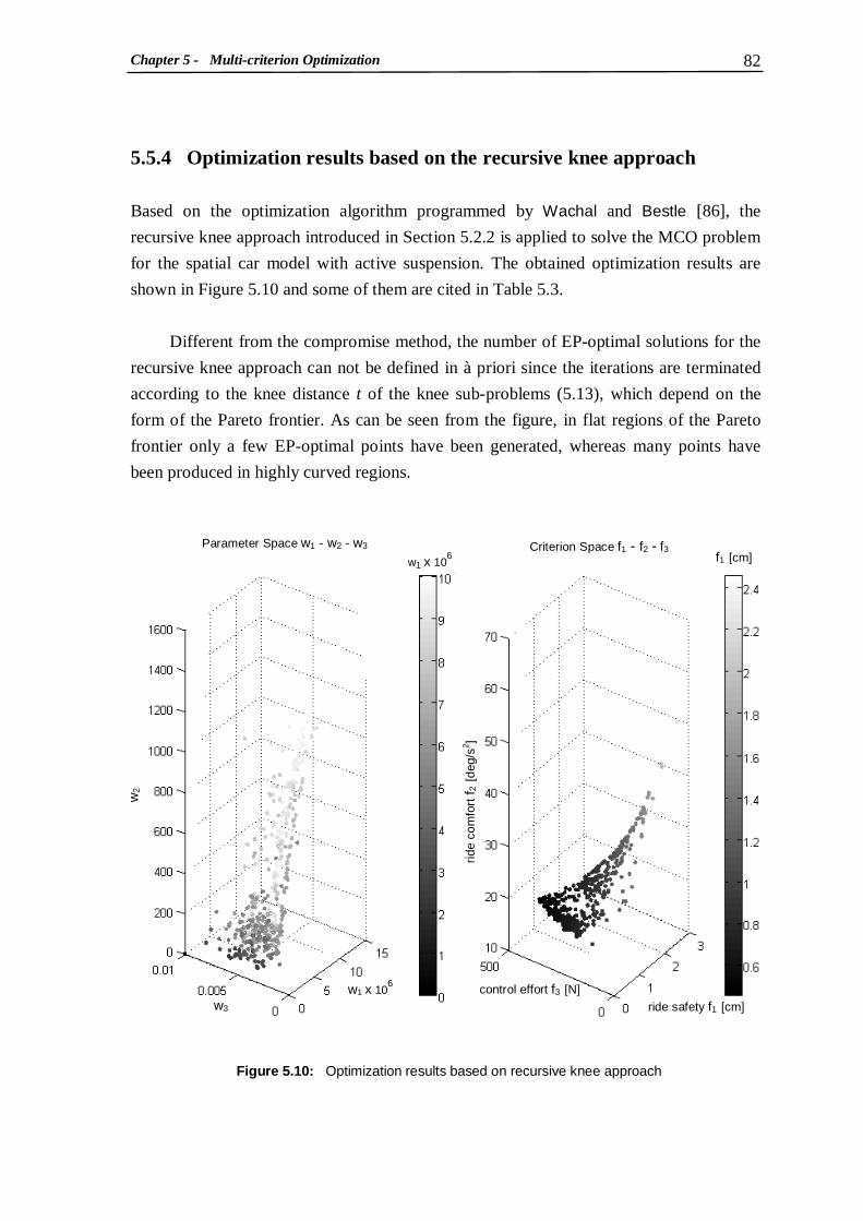
Chapter 5 - Multi-criterion Optimization 82
Figure 5.10: Optimization results based on recursive knee approach
5.5.4 Optimization results based on the recursive knee approach
Based on the optimization algorithm programmed by Wachal and Bestle [86], the
recursive knee approach introduced in Section 5.2.2 is applied to solve the MCO problem
for the spatial car model with active suspension. The obtained optimization results are
shown in Figure 5.10 and some of them are cited in Table 5.3.
Different from the compromise method, the number of EP-optimal solutions for the
recursive knee approach can not be defined in à priori since the iterations are terminated
according to the knee distance t of the knee sub-problems (5.13), which depend on the
form of the Pareto frontier. As can be seen from the figure, in flat regions of the Pareto
frontier only a few EP-optimal points have been generated, whereas many points have
been produced in highly curved regions.
w2
w1 x 106
w1 x 106
Parameter Space w1 - w2 - w3 Criterion Space f1 - f2 - f3
w3 control effort f3 [N]
ride safety f1 [cm]
ride
com
fort
f 2 [
deg/
s2 ]
f1 [cm]

Chapter 5 - Multi-criterion Optimization 83
criteria design variables
point f1
[cm]
f2
[deg/s2]
f3
[N]
w1
x104
w2
w3
x10−4
1 2 3 4 5 6 7 8 9
10 …
320 321 322 323 324 325 326 327 328 329 330
0.4541
0.4586 0.4590 0.4593 0.4597 0.4685 0.4733 0.4814 0.4817 0.4845
…
0.7857 0.7918 0.8038 0.8049 0.8292 0.8418 0.8448 0.8869 0.9819 1.0014 1.2586
17.6671 16.8939 17.0350 16.5736 16.7113 16.7059 17.1598 17.4234 16.0460 16.5221
…
30.5169 30.2930 29.7068 29.5808 31.8725 32.2900 32.5263 31.4941 36.3711 35.8023 48.1030
426.5835 423.7608 423.7857 422.5167 422.5151 415.5217 412.7485 407.0224 403.9879 402.7689
…
55.5835 53.5705 49.7925 49.4576 43.4565 40.2773 39.5997 29.7252 9.6581 7.7729
0.0000
6.9832 5.6952 5.7814 5.6077 5.7207 5.9585 5.9763 5.5970 4.5710 6.2455
…
2.7803 2.9684 3.6794 2.5385 2.9824 2.3654 2.3689 2.9643 4.2049 4.9348
0.0000
20.4031
70.6110 22.5580 12.1690 13.3746 10.5000 13.0354 18.2439 48.9117 42.8665
…
17.8988 21.4410 67.9262 51.9351 17.8921 15.7321 12.0562 97.0776 92.5754 88.5600
0.00000
0.3543 0.2881 0.2935 0.2813 0.3234 0.3371 0.3432 0.3275 0.2274 0.3173
…
0.6568 0.7175 0.9308 0.6450 0.8113 0.6718 0.6786 0.5020 0.6611 0.7065
0.0100
Since the knee of the Pareto frontier is usually located in the middle interval, the
formula (5.16) for defining starting points used in the compromise method is inefficient to
the recursive knee approach. A new formulation for defining the starting point of the knee
sub-problem (5.13) has been presented by Wachal and Bestle [86]. With this formulation,
the starting point can be changed automatically when the sub-problem (5.13) is required
to be restarted after a definite number of non-terminal computations. Another advantage
of the recursive knee approach is the Pareto filter algorithm which filters out non-EP-
optimal solutions as well as local EP-optimal solutions that may have been obtained
during the generation of candidate designs.
Table 5.3: EP-optimal solutions for active suspension optimization based on recursive knee approach
Chapter 5 - Multi-criterion Optimization 84
Unlike the compromise method, the recursive knee approach requires to solve the
single optimization problems (5.8) only once for the individual minima defining the first
CHIM. Moreover, the risk of obtaining non-EP-optimal solutions and local EP-optimal
solutions is avoided by the Pareto filter algorithm. The recursive knee approach, therefore,
reduces the computational time by about three times compared to the compromise method
while giving the same results.
Chapter 5 - Multi-criterion Optimization 85
5.5 MCO Problem for Passive and Active Suspensions
In the previous section, the active suspension has been optimized with fixed passive
suspension parameters. In order to estimate the effectiveness of optimizing the passive
and active suspensions at the same time, the three-criterion optimization problem where
both passive and active suspension parameters are considered as design variables is
introduced in this section.
5.5.1 Problem definition
With inclusion of LQR algorithm introduced in section 5.4.2, the optimal passive and
active suspension parameters for the spatial car model can be obtained by solving the
following MCO problem:
In the above formulation, the vector of design variables p1 includes the passive suspension
parameters while p2 contains weighting factors which will determine the optimal control
gains *xK and *
wK for the active suspension based on the LQR algorithm.
( ) ( ) [ ][ ] ( ){ }
[ ][ ][ ][ ][ ][ ]
( ) ( ) ( )22.5.500maxmax:
,10,10,10
,10,0,0
,15000,25000,25000,25000,2000,2000
,5000,15000,15000,15000,1000,1000
,,,
,,,,,,
0,,:
,,,,min
2882
62
1
1
33212
61
921
321
tu
h
w w
w
r r
k k b
b
where
h
f f f
−
===
==
∈=∈=
≤≤≤∈==
=∈
−
iti
Tu
Tl
Tu
Tl
T
Trfrfrf
ulTTT
T
p
p
p
p
p
p
p
ppppppp
pfpfp
�
������������
����
������������
���
��
RI
RI
RIP
P

Chapter 5 - Multi-criterion Optimization 86
Figure 5.11: Comparison between the optimized passive, optimized active and optimized passive- active suspensions
5.5.2 Optimization results
In order to derive comparable results with a reduced computational time, the compromise
method for the case of arbitrary control effort is applied to solve the problem (5.22), which is
concretized by the MATLAB.m files introduced in Appendix D.1. The optimization results
are represented by the asterisks in Figure 5.11 and given in Table 5.4. Compared to the
results obtained from optimizing the passive suspension denoted by the stars in the figure,
ride safety and ride comfort of the car are improved by about 60% and 75%, respectively.
These values are 14% and 2% better than the results derived from optimizing the active
suspension only with arbitrary control effort which are described by the six-pointed stars.
0.2 0.4 0.6 0.8 1 1.2 1.4 1.6 1.810
20
30
40
50
60
70
ride safety f1 [cm]
ride
com
fort
f 2
[de
g/s2
]
Criterion Space f1 - f
2
original passiveoptimal passiveoptimal activeoptimal passive-active
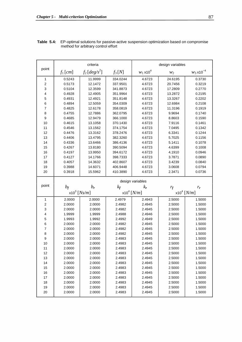
Chapter 5 - Multi-criterion Optimization 87
criteria design variables
point f1 [cm] f2 [deg/s2] f3 [N] w1 x104 w2 w3 x10−4
1 2 3 4 5 6 7 8 9
10 11 12 13 14 15 16 17 18 19 20
0.5243 0.5173 0.5104 0.4928 0.4931 0.4894 0.4825 0.4755 0.4685 0.4615 0.4546 0.4476 0.4406 0.4336 0.4267 0.4197 0.4127 0.4057 0.3988 0.3918
11.9999 12.1472 12.3599 12.4905 12.4921 12.5059 12.6178 12.7886 12.9479 13.1058 13.1562 13.3162 13.4795 13.6466 13.8180 13.9950 14.1766 14.3632 14.6071 15.5962
334.0244 337.9501 341.8873 351.9964 351.8148 354.0309 358.0819 362.0795 366.1000 370.1430 374.1754 378.2476 382.3260 386.4136 390.5094 394.6172 398.7333 402.8607 406.9448 410.3890
4.6723 4.6723 4.6723 4.6723 4.6723 4.6723 4.6723 4.6723 4.6723 4.6723 4.6723 4.6723 4.6723 4.6723 4.6723 4.6723 4.6723 4.6723 4.6723 4.6723
24.6195 20.7456 17.2809 13.2872 13.3267 12.6984 11.3196 9.9694 8.8603 7.9116 7.0495 6.3341 5.7025 5.1411 4.6399 4.1910 3.7871 3.4239 3.0608 2.3471
0.3730 0.3219 0.2770 0.2195 0.2202 0.2108 0.1919 0.1740 0.1590 0.1461 0.1342 0.1244 0.1156 0.1078 0.1008 0.0946 0.0890 0.0840 0.0794 0.0736
design variables
bf br kf kr rf rr
point
x103 [Ns/m] x104 [N/m] x104 [N/m]
1 2 3 4 5 6 7 8 9
10 11 12 13 14 15 16 17 18 19 20
2.0000 2.0000 2.0000 1.9999 1.9993 2.0000 2.0000 2.0000 2.0000 2.0000 2.0000 2.0000 2.0000 2.0000 2.0000 2.0000 2.0000 2.0000 2.0000 2.0000
2.0000 2.0000 2.0000 1.9999 1.9992 2.0000 2.0000 2.0000 2.0000 2.0000 2.0000 2.0000 2.0000 2.0000 2.0000 2.0000 2.0000 2.0000 2.0000 2.0000
2.4979 2.4982 2.4982 2.4988 2.4992 2.4982 2.4982 2.4982 2.4983 2.4983 2.4983 2.4983 2.4983 2.4983 2.4983 2.4983 2.4983 2.4983 2.4983 2.4983
2.4943 2.4945 2.4945 2.4946 2.4949 2.4945 2.4945 2.4945 2.4945 2.4945 2.4945 2.4945 2.4945 2.4945 2.4945 2.4945 2.4945 2.4945 2.4945 2.4945
2.5000 2.5000 2.5000 2.5000 2.5000 2.5000 2.5000 2.5000 2.5000 2.5000 2.5000 2.5000 2.5000 2.5000 2.5000 2.5000 2.5000 2.5000 2.5000 2.5000
1.5000 1.5000 1.5000 1.5000 1.5000 1.5000 1.5000 1.5000 1.5000 1.5000 1.5000 1.5000 1.5000 1.5000 1.5000 1.5000 1.5000 1.5000 1.5000 1.5000
Table 5.4: EP-optimal solutions for passive-active suspension optimization based on compromise method for arbitrary control effort
Chapter 5 - Multi-criterion Optimization 88
The obtained results show that the best solution for designing the active suspension
system is to optimize the parameters of both passive and active components at the same
time. However, it should be noted that the derived optimal values are valid only for a
specific operation point defined by given values of the car yaw rate and lateral
acceleration. For different operation points, the passive and active suspension parameters
have to change appropriately. Since the passive suspension parameters are typically
unchangeable, the practical way is to design a controller that is able to change its
parameters according to the changes of the system’s varying parameters. The process of
defining such a controller is known as gain-scheduling control design which will be
introduced in the next chapter in more details.

Chapter 6 - Gain-scheduling Control 89
Chapter 6
Gain-scheduling Control
Gain-scheduling is one of the most common control techniques used to design controllers
that can change their parameters in response to the variation of the system dynamics
resulting from varying parameters. In this chapter, gain-scheduling control will be
designed for the spatial car model. By considering the effects of suspension and tire
deformation on the vehicle stability in cornering situations, the operation region of the
spatial car model will be determined. Based on optimal local controllers defined for
selected operation points, the parameter-dependent controller will be then designed. The
effectiveness of the designed parameter-dependent controller will be demonstrated
through the simulation of double-lane-change maneuvers, which are designated as
standard vehicle handling tests. In order to find optimal paths for the double-lane-change
maneuvers that minimize the vehicle lateral dynamics during the test, a path generation
problem will be formulated and solved in this chapter.
6.1 Operation Region of the Spatial Car Model
As indicated in Chapter 3, the linear parameter-varying (LPV) spatial car model (3.76)
can be simplified as a set of linear time-invariant (LTI) systems (3.78) defined by
pairs( )ya,γ& . In this section, upper bounds for the lateral acceleration ay and yaw rateγ& ,
which determine the operation region of the spatial car model, will be defined based on
the stability condition of vehicles in cornering, taking into account the compliance of
suspension and tires.

Chapter 6 - Gain-scheduling Control 90
6.1.1 Vehicle side-slip and rollover stability
When cornering with large lateral acceleration, the car may slip sideways or roll over under
the action of the centrifugal force located at the car center of gravity. The most traditional
analysis of vehicle side-slip and rollover stability is based on a rigid vehicle model in
steady-state cornering as shown in Figure 6.1.
During cornering, the centrifugal force mS ay is counterbalanced by the lateral tire
forces, which are limited by values proportional to the corresponding normal tire loads and
the tire-ground friction coefficient, Mitschke [51] and Steinberg [77]. It is assumed that the
road friction coefficients µy are the same for all four wheels, resulting in
where g = 9.81 m/s2 is the gravitational acceleration. For dry-asphalt roads, the friction
coefficient is approximately µy = 1.0 resulting in a maximum lateral acceleration value
ay ≤ ay slip = 9.81 m/s2 that the car is able to reach before slipping sideways.
Figure 6.1: Rigid vehicle model
( )( )1.6
or
inoutinout
g a
g m F F F F a m
----
yslipy
SyzzyyyyS
µ
µµ
≤
=+≤+=
µy
TC tw
C
zC
yC
mS g
mS ay
hC
Fy -out Fy -in
Fz -in Fz -out
µy
tw
Chapter 6 - Gain-scheduling Control 91
The vehicle rollover threshold is defined from the two-wheel lift condition, i.e. the
normal loads on the inside wheels reach zeros, and thus the total normal load on the inside
wheels is Fz-in = 0. Taking moments about the center of contact patches for the outside
wheels TC with the simplification of the same front and rear half-track width, twf = twr = tw,
results in the simple formula for the lateral acceleration at the rollover threshold:
where hC is the static height of car’s CG above ground. The ratio (tw/hC) is often referred to
as the static stability factor used to estimate roughly the vehicle rollover-resistance ability.
The maximum lateral acceleration uya of the car during cornering is limited by the
smaller one of the lateral accelerations at the rollover and side-slip threshold, i.e.
For the spatial car model with the dates given in Appendix A, ay roll = 14.91 m/s2 is greater
than ay slip = 9.81 m/s2, which means that the car will more probably slip sideways instead of
rolling over.
However, neglecting the deformation of suspension and tires in the above analysis
often leads to overestimation of the rollover threshold. To determine more accurately the
upper bound for the lateral acceleration, the influences of suspension and tire compliance
on the vehicle rollover stability must be considered.
6.1.2 Effects of suspension and tires compliance
Due to lateral compliance of suspension and tires, the distance in lateral direction between
the center-plane of the vehicle and the tire contact patches is changed, usually reduced. In
addition, the transmission of lateral forces between the body and the wheels results in
vertical components called “jacking” forces, which in general do not cancel out and
usually increase the static height of car’s CG. The changes in effective half-track width
and height of car’s CG, which reduce the lateral acceleration at the rollover threshold, are
illustrated in Figure 6.2.
( ) ( )3.6.,min a a a slipyy rolluy =
( )2.6 g h
t a a oll
C
wryy =≤
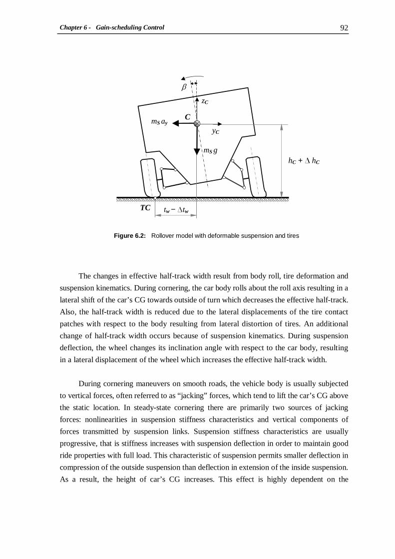
Chapter 6 - Gain-scheduling Control 92
The changes in effective half-track width result from body roll, tire deformation and
suspension kinematics. During cornering, the car body rolls about the roll axis resulting in a
lateral shift of the car’s CG towards outside of turn which decreases the effective half-track.
Also, the half-track width is reduced due to the lateral displacements of the tire contact
patches with respect to the body resulting from lateral distortion of tires. An additional
change of half-track width occurs because of suspension kinematics. During suspension
deflection, the wheel changes its inclination angle with respect to the car body, resulting
in a lateral displacement of the wheel which increases the effective half-track width.
During cornering maneuvers on smooth roads, the vehicle body is usually subjected
to vertical forces, often referred to as “jacking” forces, which tend to lift the car’s CG above
the static location. In steady-state cornering there are primarily two sources of jacking
forces: nonlinearities in suspension stiffness characteristics and vertical components of
forces transmitted by suspension links. Suspension stiffness characteristics are usually
progressive, that is stiffness increases with suspension deflection in order to maintain good
ride properties with full load. This characteristic of suspension permits smaller deflection in
compression of the outside suspension than deflection in extension of the inside suspension.
As a result, the height of car’s CG increases. This effect is highly dependent on the
Figure 6.2: Rollover model with deformable suspension and tires
tw − ∆tw
hC + ∆ hC
TC
mS g
mS ay C
zC
yC
β

Chapter 6 - Gain-scheduling Control 93
particular stiffness characteristic, which is difficult to be captured in a general approach.
Therefore, it is often neglected in the analysis of influences of suspension compliance on
the vehicle rollover stability. The second jacking effect is a result of forces in suspension
links. Lateral forces generated during cornering maneuvers are transmitted between the
body and the wheels through relatively rigid suspension links, which are in general not
parallel to the ground. Therefore, the reaction forces in these elements have vertical
components resulting in a vertical net force, which usually pushes the body up for typical
suspensions.
Hac [35] shows that the effect of total change in the effective half-track width
resulting from body roll, tire compliance and suspension kinematics reduces the lateral
acceleration at the rollover threshold computed by the static stability factor (6.2) by about
15%, while the change in height of car’s CG caused by jacking forces contributes a
reduction of about 5% for passenger cars. Applying these results to the spatial car model
yields the lateral acceleration at the rollover threshold ay roll ≈ 11.93 m/s2. This result is
limited to the passive suspension system. When the active suspension system is applied,
the suspension deformation will be restrained significantly by the controlled forces
generated by the active dampers at four wheels. In this case, the value of ay roll will be
between 11.93 −14.91 m/s2.
Since the lateral acceleration at the rollover threshold is greater than that at the side-
slip threshold, the upper bound value of the lateral acceleration for the spatial car model is
determined as ayu = ay slip = 9.81 m/s2.
6.1.3 Definition of operation region and operation points
Theoretically, the operation region of the spatial car model is a rectangle bounded by the
coordinate axes and the upper bounds for lateral acceleration ayu and yaw rate uγ& as
illustrated in Figure 6.3, where ayu = 9.81 m/s2 is the maximum lateral acceleration that the
car is able to reach before slipping sideways, while uγ& can be computed from ayu and the
car minimum turning radius Rmin as
( ) R
a 4.6.
min
uyu
=γ&

Chapter 6 - Gain-scheduling Control 94
This equation is obtained from (3.51) in the limit case uuuy γγ && Rv va minand == . With
Rmin = 10 m, the upper bound of yaw rate is derived as uγ& ≈ 1.0 rad/s. In practice, this
operation region may be further reduced by minimum turning radius and maximum
velocity as ay ≤ γ& vmax , however, in order to simplify the computational procedure, the
whole operation region as shown in Figure 6.3 will be used to design gain-scheduling
control for the spatial car model.
The variation of the car yaw rate γ& and lateral acceleration ay in the operation
region leads to changes in the system dynamics. To maintain the required performance of
the system, the controllers have to update their parameters on-line according to varying
system parameters. Thus, a parameter-dependent state-feedback gain matrix ( )yxK a,γ&
and disturbance-feed forward gain vector ( )ywK a,γ& are required to control the spatial car
model. To design such a controller, the dependence of the controller on the variation of γ&
and ay over the operation region must be investigated. For this purpose, 66 pairs ( )ya,γ&
corresponding to 66 operation points are selected as illustrated by the small circles in
Figure 6.3. Each operation point defines a linear time-invariant system, whose optimal
controllers can be obtained by applying the multi-criterion optimization method with the
linear quadratic regulator algorithm as introduced in the previous chapter.
Figure 6.3: Operation region and selected operation points
[ ]rad/s γ&
1.00=uγ&
][ 2m/s a y9.81=uya0
0.2
0.4
0.6
0.8

Chapter 6 - Gain-scheduling Control 95
6.2 Gain-scheduling Design for the Spatial Car Model
In this section, the optimal local controllers, i.e. the optimal state-feedback gain matrices
and disturbance-feed forward gain vectors of the linear time-invariant systems defined by
the selected operation points, will be computed. The negligible influence of the yaw rate
on the optimal local controllers will be shown. Based on the variation laws of the
components of the optimal local controllers, the parameter-dependent controller as
continuous functions of the lateral acceleration will be formulated. 6.2.1 Optimal local controllers
In order to simplify the problem of finding the optimal local controllers, a scalar
optimization problem is used instead of the multi-criterion optimization problem. Since ride
safety is most important for cars in cornering, this criterion is defined as the only objective
for the gain-scheduling design:
where the vector of design variables p and the feasible design space P are defined
according to (5.18). The optimal state-feedback gain matrix Kx and disturbance-feed
forward gain vector Kw are derived from the optimal solution of problem (6.5) based on a
strategy similar to the one shown in Figure 5.8.
Figure 6.4 shows the obtained results for the selected operation points, which are
generated by changing evenly lateral acceleration ay while keeping constant yaw rateγ& .
The small figures describe the dependences of the optimal control gains Kx and Kw on
lateral acceleration and yaw rate. As can be seen from the figures, the obtained optimal
local controllers depend only slightly on the yaw rate. This can be explained by the
negligible effect of yaw rate on the car ride safety criterion as follows:
With values 0.1≤γ& rad/s for the yaw rate and the parameters of the car given in
Appendix A.1, the yaw rate-dependent matrices( )γ&P in (3.56) and ( )γ&Q in (3.57)
(with 0and0 == γ&& ax ) are much smaller than the invariant matrices TSSS GBG and
( ) TSASS GKKG + in the state equations (3.74), respectively. The matrices ( )γ&P and
( ) ( ) ( )5.6411,4
1min
0
4
1
211
i
dt tz T
f where f
==∈
∫ ∑=
T
iSi
p P

Chapter 6 - Gain-scheduling Control 96
( )γ&Q , therefore, can be omitted in the matrices ( )γ&A and ( )γ&C defined in equations
(3.74) and (3.75), i.e.
Thus, the linear system (3.76) can be substituted by
Figure 6.4: Components of optimal gains *xK and *
wK vs. ay for differentγ&
( ) ( )
( ) ( ) ( )6.6.:
and:
110
110
−+−=≈
−+−=≈
−−
−−
TSSS
TTSASS
T
TSSS
TSASS
GBGMgGKKGMg
I0CC
GBGMGKKGM
I0AA
ββγ
γ
&&&&
&
&
( )( )
( )7.6
.
,
0
0
aw
aw
++≈
++≈
yw
yw
duDxCy
buBxAx&
0
5x 10
4
kx 11
γ = 0.0γ = 0.2γ = 0.4γ = 0.6γ = 0.8γ = 1.0
kx 21
kx 31
kx 41
-2
0
2x 10
4
kx 12
kx 22
kx 32
kx 42
-505
10x 10
4
kx 13 k
x 23
kx 33 k
x 43
0
5000
kx 14
kx 24 k
x 34
kx 44
-5000
0
5000
kx 15
kx 25
kx 35
kx 45
-5000
0
5000k
x 16
kx 26
kx 36
kx 46
0 5 10-200
0
200
ay [m/s2]
kw 1
0 5 10
ay [m/s2]
kw 2
0 5 10
ay [m/s2]
kw 3
0 5 10
ay [m/s2]
kw 4
.
.
.
.
.
.
T
xK *
T
wK *
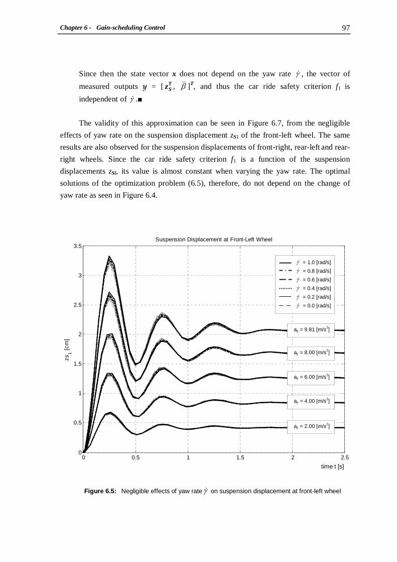
Chapter 6 - Gain-scheduling Control 97
Since then the state vector x does not depend on the yaw rate γ& , the vector of
measured outputs y = [ β&& ,TSz ]T, and thus the car ride safety criterion f1 is
independent of γ& .■
The validity of this approximation can be seen in Figure 6.7, from the negligible
effects of yaw rate on the suspension displacement zS1 of the front-left wheel. The same
results are also observed for the suspension displacements of front-right, rear-left and rear-
right wheels. Since the car ride safety criterion f1 is a function of the suspension
displacements zSi, its value is almost constant when varying the yaw rate. The optimal
solutions of the optimization problem (6.5), therefore, do not depend on the change of
yaw rate as seen in Figure 6.4.
Figure 6.5: Negligible effects of yaw rateγ& on suspension displacement at front-left wheel
0 0.5 1 1.5 2 2.50
0.5
1
1.5
2
2.5
3
3.5Suspension Displacement at Front-Left Wheel
Time [s]
zs1 [
cm]
ay = 9.81 [m/s2]
γ& = 1.0 [rad/s]
γ& = 0.8 [rad/s]
γ& = 0.6 [rad/s]
γ& = 0.4 [rad/s]
γ& = 0.2 [rad/s]
γ& = 0.0 [rad/s]
ay = 8.00 [m/s2]
ay = 6.00 [m/s2]
ay = 4.00 [m/s2]
ay = 2.00 [m/s2]
time t [s]

Chapter 6 - Gain-scheduling Control 98
6.2.2 Parameter-dependent controller design
As discussed above, the effect of the yaw rate on the optimal local controllers can be
neglected. However, to design an adequate mean controller, the mean values of the
optimal local controllers obtained from six different values of yaw rate are used for the
parameter-dependent controller of the spatial car model. The values of the control gains
are given in Table 6.1 and shown by the dots in Figure 6.6. In order to obtain
continuously varying functions of the lateral acceleration, polynomials in ay fitting the
mean values of the optimal local controllers have to be found.
Figure 6.6: Mean-value points and interpolated curves for control gains
0
5x 10
4
kx 11
kx 21 k
x 31 k
x 41
-2
0
2x 10
4
kx 12
kx 22
kx 32
kx 42
-505
10x 10
4
kx 13 k
x 23
kx 33
kx 43
0
5000
kx 14
kx 24
kx 34
kx 44
-5000
0
5000
kx 15
kx 25
kx 35
kx 45
-5000
0
5000k
x 16
kx 26
kx 36
kx 46
0 5 10-200
0
200
ay [m/s2]
kw 1
0 5 10
ay [m/s2]
kw 2
0 5 10
ay [m/s2]
kw
3
0 5 10
ay [m/s2]
kw 4
kx 43
kx 44
kx 45
kx 46
TxK *
TwK *

Chapter 6 - Gain-scheduling Control 99
lateral acceleration ay [m/s2]
0.0000 0.9810 1.9620 2.9430 4.9050 4.9050 5.8860 6.8670 7.8480 8.8290 9.8100
kx 11 kx 12 kx 13 kx 14 kx 15 kx 16
kx 21 kx 22 kx 23 kx 24 kx 25 kx 26
kx 31 kx 32 kx 33 kx 34 kx 35 kx 36
kx 41 kx 42 kx 43 kx 44 kx 45 kx 46
kw1
kw2
kw3
kw4
3.8874
1.6879
-4.0186
0.4892
0.1943
-0.4668
3.8959
-1.8095
-3.8193
0.4887
-0.1934
-0.4674
4.0485
1.8045
7.2091
0.3254
0.1919
0.5604
4.0569
-1.6653
7.4068
0.3249
-0.1927
0.5598
0.0091
-0.0104
0.0102
-0.0091
3.8833
1.6858
-4.0143
0.4889
0.1941
-0.4665
3.8917
-1.8073
-3.8152
0.4884
-0.1932
-0.4671
4.0443
1.8024
7.2016
0.3252
0.1917
0.5600
4.0527
-1.6633
7.3991
0.3247
-0.1926
0.5594
0.0091
-0.0103
0.0102
-0.0090
3.8833
1.6859
-4.0143
0.4889
0.1941
-0.4665
3.8917
-1.8074
-3.8153
0.4884
-0.1932
-0.4671
4.0443
1.8024
7.2017
0.3252
0.1917
0.5600
4.0527
-1.6633
7.3991
0.3247
-0.1926
0.5594
0.0091
-0.0103
0.0102
-0.0090
3.8833
1.6858
-4.0143
0.4889
0.1941
-0.4665
3.8917
-1.8073
-3.8152
0.4884
-0.1932
-0.4671
4.0443
1.8024
7.2016
0.3252
0.1917
0.5600
4.0527
-1.6632
7.3991
0.3247
-0.1926
0.5594
0.0091
-0.0103
0.0102
-0.0090
3.8813
1.6846
-4.0123
0.4887
0.1941
-0.4663
3.8897
-1.8062
-3.8132
0.4882
-0.1931
-0.4669
4.0423
1.8012
7.1980
0.3251
0.1916
0.5598
4.0507
-1.6621
7.3955
0.3246
-0.1925
0.5592
0.0091
-0.0103
0.0102
-0.0090
3.8822
1.6516
-4.0111
0.4888
0.1946
-0.4663
3.8904
-1.7716
-3.8162
0.4883
-0.1937
-0.4672
4.0433
1.7667
7.2016
0.3252
0.1922
0.5601
4.0514
-1.6295
7.3950
0.3247
-0.1930
0.5592
0.0087
-0.0100
0.0099
-0.0087
3.3479
1.4313
-3.4292
0.4462
0.1714
-0.4259
3.3522
-1.4987
-3.3227
0.4459
-0.1709
-0.4261
3.5008
1.4920
6.2683
0.2948
0.1696
0.5076
3.5051
-1.4149
6.3740
0.2945
-0.1700
0.5073
0.0067
-0.0075
0.0074
-0.0067
2.7419
1.1867
-2.7747
0.3913
0.1429
-0.3734
2.7427
-1.2005
-2.7539
0.3912
-0.1428
-0.3734
2.8820
1.1920
5.1940
0.2563
0.1417
0.4411
2.8828
-1.1763
5.2147
0.2563
-0.1418
0.4410
0.0053
-0.0055
0.0055
-0.0053
2.3430
1.0060
-2.3615
0.3544
0.1238
-0.3380
2.3430
-1.0060
-2.3615
0.3544
-0.1238
-0.3380
2.4743
0.9980
4.4687
0.2304
0.1228
0.3961
2.4743
-0.9980
4.4687
0.2304
-0.1228
0.3961
0.0042
-0.0042
0.0041
-0.0041
2.0516
0.8560
-2.0672
0.3257
0.1099
-0.3104
2.0516
-0.8560
-2.0672
0.3257
-0.1099
-0.3104
2.1754
0.8492
3.9294
0.2103
0.1090
0.3613
2.1754
-0.8492
3.9294
0.2103
-0.1090
0.3613
0.0033
-0.0033
0.0033
-0.0033
1.8212
0.7414
-1.8344
0.3016
0.0987
-0.2872
1.8212
-0.7414
-1.8344
0.3016
-0.0987
-0.2872
1.9381
0.7356
3.5014
0.1936
0.0979
0.3322
1.9381
-0.7356
3.5014
0.1936
-0.0979
0.3322
0.0028
-0.0028
0.0027
-0.0027
Table 6.1: Mean values of the optimal local controllers (x104)

Chapter 6 - Gain-scheduling Control 100
This is achieved with the MATLAB function “polyfit”, which finds the
coefficients of a polynomial p(x) of order n in a least-mean-square sense. To reduce the
order of the interpolation functions, the fitting curves illustrated in Figure 6.6 are
divided into two parts, respectively: 1) curve segments corresponding to ay > 4.905 m/s2
which are represented by fourth-order polynomial functions of the form ( ) 542
33
24
1 c ac ac ac ac ap ++++= yyyyy , and 2) straight-line segments for ay ≤ 4.905
m/s2 with magnitudes defined from the associated polynomial functions for p(ay = 4.905).
The coefficients of the fourth-order polynomials functions are given in Table 6.2.
for ay ≤ 4.905 m/s2 for ay > 4.905 m/s2
( ) 542
33
24
1 c ac ac ac ac apk ++++== yyyyy
parameter-dependent controller
x 104
c1 c2 x 103 c3 x 10
4 c4 x 105 c5 x 10
5
kx 11 kx 12 kx 13 kx 14 kx 15 kx 16
3.8822
1.6516
-4.0111
0.4888
0.1946
-0.4663
-73.1516
-18.8070
83.4862
-7.6396
-3.8878
7.3274
2.1885
0.5730
-2.4868
0.2303
0.1171
-0.2210
-2.3554
-0.6248
2.6637
-0.2514
-0.1275
0.2416
1.0330
0.2687
-1.1650
0.1136
0.0573
-0.1094
-1.1707
-0.2169
1.3555
-0.1310
-0.0703
0.1269
kx 21 kx 22 kx 23 kx 24 kx 25 kx 26
3.8904
-1.7716
-3.8162
0.4883
-0.1937
-0.4672
-73.9046
31.0983
64.7866
-7.5834
3.7921
7.2557
2.2100
-0.9276
-1.9508
0.2286
-0.1144
-0.2187
-2.3772
0.9914
2.1147
-0.2497
0.1247
0.2388
1.0421
-0.4261
-0.9328
0.1129
-0.0560
-0.1078
-1.1831
0.4421
1.0329
-0.1299
0.0685
0.1237 kx 31
kx 32 kx 33 kx 34 kx 35 kx 36
4.0433
1.7667
7.2016
0.3252
0.1922
0.5601
-75.2145
-31.8039
-127.0284
-5.2403
-3.7701
-8.9698
2.2511
0.9477
3.8142
0.1579
0.1137
0.2703
-2.4246
-1.0120
-4.1235
-0.1722
-0.1239
-0.2950
1.0651
0.4349
1.8172
0.0776
0.0557
0.1329
-1.2076
-0.4562
-2.0378
-0.0898
-0.0682
-0.1533
Table 6.2: Interpolated functions for the gain matrices of the parameter-dependent controller
Kx

Chapter 6 - Gain-scheduling Control 101
kx 41 kx 42 kx 43 kx 44 kx 45 kx 46
4.0514
-1.6295
7.3950
0.3247
-0.1930
0.5592
-75.9615
17.7079
-145.5807
-5.1845
3.8492
-9.0409
2.2724
-0.5411
4.3460
0.1563
-0.1160
0.2727
-2.4463
0.5915
-4.6682
-0.1705
0.1263
-0.2978
1.0742
-0.2544
2.0475
0.0769
-0.0567
0.1344
-1.2199
0.1977
-2.3579
-0.0887
0.0695
-0.1564
Kw
kw 1 kw 2 kw 3 kw 4
0.0087
-0.0100
0.0099
-0.0087
0.0987
0.0704
-0.0573
-0.0854
-0.0031
-0.0019
0.0015
0.0027
0.0037
0.0016
-0.0012
-0.0033
-0.0021
-0.0003
0.0001
0.0019
0.0055
-0.0017
0.0021
-0.0051
6.3 Vehicle Handling Test Simulation
The control above has been designed for constant yaw rates and lateral accelerations. In
order to see the effectiveness of the designed gain-scheduling control on ride safety and
ride comfort, a double-lane-change maneuver as one of the standard handling tests for
vehicles will be simulated. The path for the maneuver will be generated as optimal path
minimizing the lateral acceleration.
6.3.1 Double-lane-change maneuvers
There are two types of double-lane-change maneuvers: one developed by the International
Organization for Standardization (ISO) and one introduced by the Consumers Union (CU).
• ISO 3888-2 double-lane-change maneuver
The ISO 3888-2 double-lane-change maneuver, which is also known as the “Elk” or
“Moose” avoidance test, represents a changing vehicle path based on pre-determined cone
placement on the road as illustrated in Figure 6.7.

Chapter 6 - Gain-scheduling Control 102
The widths of the run-up section and swerve section are calculated as functions of the
vehicle width. The cone sections must be handled under overrun conditions, i.e. the
throttle must be released on entering the section and the car must be in its top gear (or
position "D" for vehicles with automatic transmission). The entrance speed is at least
v = 60 km/h. These conditions significantly reduce the possibility of driver influence. The
test is considered to be passed if no cones are knocked over, and the maneuver is carried
out on a dry road.
• Consumers Union Short Course double-lane-change maneuver
The Consumers Union Short Course double-lane-change maneuver is designed to test
object avoidance. The schematic of this maneuver is sketched in Figure 6.8. In testing the
vehicle is required to exit the original lane to avoid a road obstruction and immediately
returns to the original lane without knocking out the cones. Like for the ISO 3888-2
maneuver, the Consumers Union Short Course double-lane-change maneuver is
performed on dry road with a minimal entrance speed of v = 60 km/h.
Figure 6.7: ISO 3888-2 double-lane-change maneuver
path of vehicle
throttle released
A
B 2 m
12 m 13.5 m 12 m
1 m
3 m
cone
v
A = 1.1 x Vehicle Width + 0.25 m
B = Vehicle Width + 1 m
11 m 12.5 m
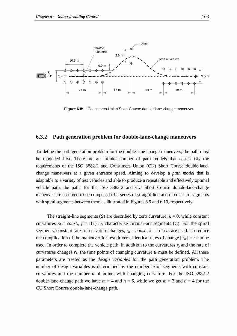
Chapter 6 - Gain-scheduling Control 103
6.3.2 Path generation problem for double-lane-change maneuvers
To define the path generation problem for the double-lane-change maneuvers, the path must
be modelled first. There are an infinite number of path models that can satisfy the
requirements of the ISO 3882-2 and Consumers Union (CU) Short Course double-lane-
change maneuvers at a given entrance speed. Aiming to develop a path model that is
adaptable to a variety of test vehicles and able to produce a repeatable and effectively optimal
vehicle path, the paths for the ISO 3882-2 and CU Short Course double-lane-change
maneuver are assumed to be composed of a series of straight-line and circular-arc segments
with spiral segments between them as illustrated in Figures 6.9 and 6.10, respectively.
The straight-line segments (S) are described by zero curvature, κ = 0, while constant
curvatures κj = const., j = 1(1) m, characterize circular-arc segments (C). For the spiral
segments, constant rates of curvature changes, rk = const., k = 1(1) n, are used. To reduce
the complication of the maneuver for test drivers, identical rates of change | rk | = r can be
used. In order to complete the vehicle path, in addition to the curvatures κj and the rate of
curvatures changes rk, the time points of changing curvature tk must be defined. All these
parameters are treated as the design variables for the path generation problem. The
number of design variables is determined by the number m of segments with constant
curvatures and the number n of points with changing curvature. For the ISO 3882-2
double-lane-change path we have m = 4 and n = 6, while we get m = 3 and n = 4 for the
CU Short Course double-lane-change path.
Figure 6.8: Consumers Union Short Course double-lane-change maneuver
21 m 18 m 18 m
cone
v
10.5 m
3.6 m
0.9 m
throttle released
15 m
3.6 m
2.4 m
path of vehicle

Chapter 6 - Gain-scheduling Control 104
Figure 6.10: Path model for CU Short Course double-lane-change maneuver
Figure 6.9: Path model for ISO 3882-2 double-lane-change maneuver
B
2 m
3 m
κ [m−1]
κ1
r2 r5
κ4
S C
C
C S
time t [s] t1 t2
r3
κ2
r4
κ3
t6 t5 t3 t4
r1 r6
C S
κ [m−1]
t1
κ1 κ3
t4
κ2
t2 t3
r2 r3
S C C
S
C
r1 r4
time t [s]
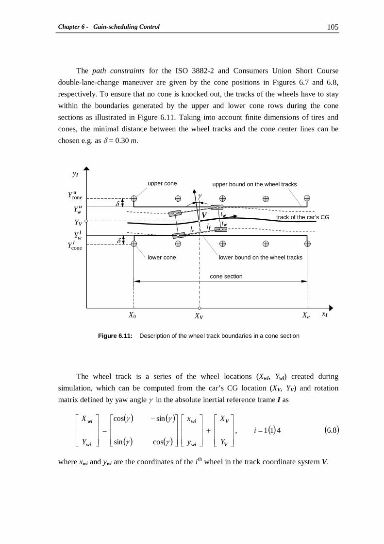
Chapter 6 - Gain-scheduling Control 105
The path constraints for the ISO 3882-2 and Consumers Union Short Course
double-lane-change maneuver are given by the cone positions in Figures 6.7 and 6.8,
respectively. To ensure that no cone is knocked out, the tracks of the wheels have to stay
within the boundaries generated by the upper and lower cone rows during the cone
sections as illustrated in Figure 6.11. Taking into account finite dimensions of tires and
cones, the minimal distance between the wheel tracks and the cone center lines can be
chosen e.g. as δ = 0.30 m.
The wheel track is a series of the wheel locations (Xwi, Ywi) created during
simulation, which can be computed from the car’s CG location (XV, YV) and rotation
matrix defined by yaw angle γ in the absolute inertial reference frame I as
where xwi and ywi are the coordinates of the ith wheel in the track coordinate system V.
Figure 6.11: Description of the wheel track boundaries in a cone section
( ) ( )( ) ( )
( ) ( )8.6411,
cossin
sincos
i
Y
X
y
x
Y
X
=
+
−=
V
V
wi
wi
wi
wi
γγ
γγ
XV
YV
γ
tw
lf lr tw
V
lower cone
upper cone upper bound on the wheel tracks
lower bound on the wheel tracks
δ
cone section
yI
xI
uconeY
lconeY
δ
X0 Xe
track of the car’s CG
lwY
uwY

Chapter 6 - Gain-scheduling Control 106
Tables 6.3 and 6.4 show the section dimensions of the ISO 3882-2 and Consumers Union
(CU) Short Course double-lane-change (DLC) maneuver and the wheel track boundaries
for the studied car where the vehicle width is assumed to be 2.05 m. It should be noted
that for both types of double-lane-change maneuvers the test requires that the car
maintains a straight trajectory only within the first cone section of the course. The car’s
heading orientation is unrestricted at the end of the test. For none-cone sections, no
bounds on the wheel tracks are required. Based on the parameters given in the tables, the
constraints on the wheel tracks for the cone sections 1, 3 and 5 can be formulated as
shown in Table 6.5.
position section 1 section 2 section 3 section 4 section 5
X0 [m] 10.0 22.0 35.5 46.5 59.0
Xe [m] 22.0 35.5 46.5 59.0 71.0
uconeY [m] 1.25 5.30 1.50 l
coneY [m] -1.25 2.25 -1.50
uwY [m] 0.95 5.00 1.20 l
wY [m] -0.95 2.55 -1.20
position section 1 section 2 section 3 section 4 section 5
X0 [m] 10.0 31.0 46.0 46.0 64.0
Xe [m] 31.0 46.0 46.0 64.0 82.0
uconeY [m] 1.20 5.70 1.80 l
coneY [m] -1.20 2.10 -1.80
uwY [m] 0.90 5.40 1.50 l
wY [m] -0.90 2.40 -1.50
Table 6.3: Section dimensions and wheel track boundaries for ISO 3882-2 DLC maneuver
Table 6.4: Section dimensions and wheel-track boundaries for CU Short Course DLC maneuver
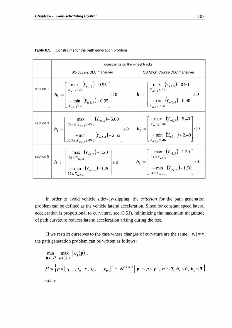
Chapter 6 - Gain-scheduling Control 107
constraints on the wheel tracks
ISO 3882-2 DLC maneuver CU Short Course DLC maneuver
section 1
section 3
section 5
In order to avoid vehicle sideway-slipping, the criterion for the path generation
problem can be defined as the vehicle lateral acceleration. Since for constant speed lateral
acceleration is proportional to curvature, see (3.51), minimizing the maximum magnitude
of path curvature reduces lateral acceleration arising during the test.
If we restrict ourselves to the case where changes of curvature are the same, | rk | = r,
the path generation problem can be written as follows:
( )( )
[ ]{ }where
r
t
t
mn
0 h0h0hpppp
pp
ulTmn
j mj
≤≤≤≤≤∈==
∈
++
=
3211
11
11
,,,...,,,,...,,:
,maxmin
RIκκ
κ
P
P
( )( ) 0
95.0min
95.0max
:
4,2
3,1
1
22
22
4,2
3,1
Y
Y
X
X
≤
−−
−=
≤
≤
w
w
w
w
h
( )( ) 0
55.2min
00.5max
:
4,2
3,1
2
5.465.35
5.465.35
4,2
3,1
Y
Y
X
X
≤
+−
−=
≤≤
≤≤
w
w
w
w
h
( )( ) 0
20.1min
20.1max
:
4,2
3,1
3
4,2
3,1
59
59
Y
Y
X
X
≤
−−
−=
≤
≤
w
w
w
w
h
( )( ) 0
90.0max
90.0max
:
4,2
3,1
1
31
31
4,2
3,1
Y
Y
X
X
≤
−
−=
≤
≤
w
w
w
wh
( )( ) 0
40.2min
40.5max
:
4,2
3,1
2
46
46
4,2
3,1
Y
Y
X
X
≤
+=−
−==
w
w
w
w
h
( )( ) 0
50.1min
50.1max
:
4,2
3,1
3
4,2
3,1
64
64
Y
Y
X
X
≤
−−
−=
≤
≤
w
w
w
w
h
Table 6.5: Constraints for the path generation problem
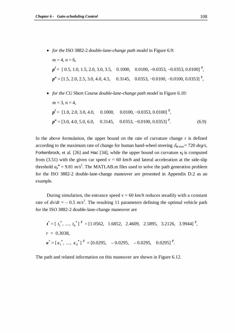
Chapter 6 - Gain-scheduling Control 108
• for the ISO 3882-2 double-lane-change path model in Figure 6.9:
m = 4, n = 6,
pl = [ 0.5, 1.0, 1.5, 2.0, 3.0, 3.5, 0.1000, 0.0100, −0.0353, −0.0353, 0.0100] T,
pu = [1.5, 2.0, 2.5, 3.0, 4.0, 4.5, 0.3145, 0.0353, −0.0100, −0.0100, 0.0353] T,
• for the CU Short Course double-lane-change path model in Figure 6.10:
m = 3, n = 4,
pl = [1.0, 2.0, 3.0, 4.0, 0.1000, 0.0100, −0.0353, 0.0100] T,
pu = [3.0, 4.0, 5.0, 6.0, 0.3145, 0.0353, −0.0100, 0.0353] T. (6.9)
In the above formulation, the upper bound on the rate of curvature change r is defined
according to the maximum rate of change for human hand-wheel steering δst max= 720 deg/s,
Forkenbrock, et al. [26] and Hac [34], while the upper bound on curvature κj is computed
from (3.51) with the given car speed v = 60 km/h and lateral acceleration at the side-slip
threshold ayu = 9.81 m/s2. The MATLAB.m files used to solve the path generation problem
for the ISO 3882-2 double-lane-change maneuver are presented in Appendix D.2 as an
example.
During simulation, the entrance speed v = 60 km/h reduces steadily with a constant
rate of dv/dt = – 0.5 m/s2. The resulting 11 parameters defining the optimal vehicle path
for the ISO 3882-2 double-lane-change maneuver are
t* = [ **61 ,..., t t ] T = [1.0562, 1.6852, 2.4609, 2.5895, 3.2126, 3.9944] T,
r = 0.3038,
κ* = [ **41 ,..., κκ ] T = [0.0295, – 0.0295, – 0.0295, 0.0295] T.
The path and related information on this maneuver are shown in Figure 6.12.
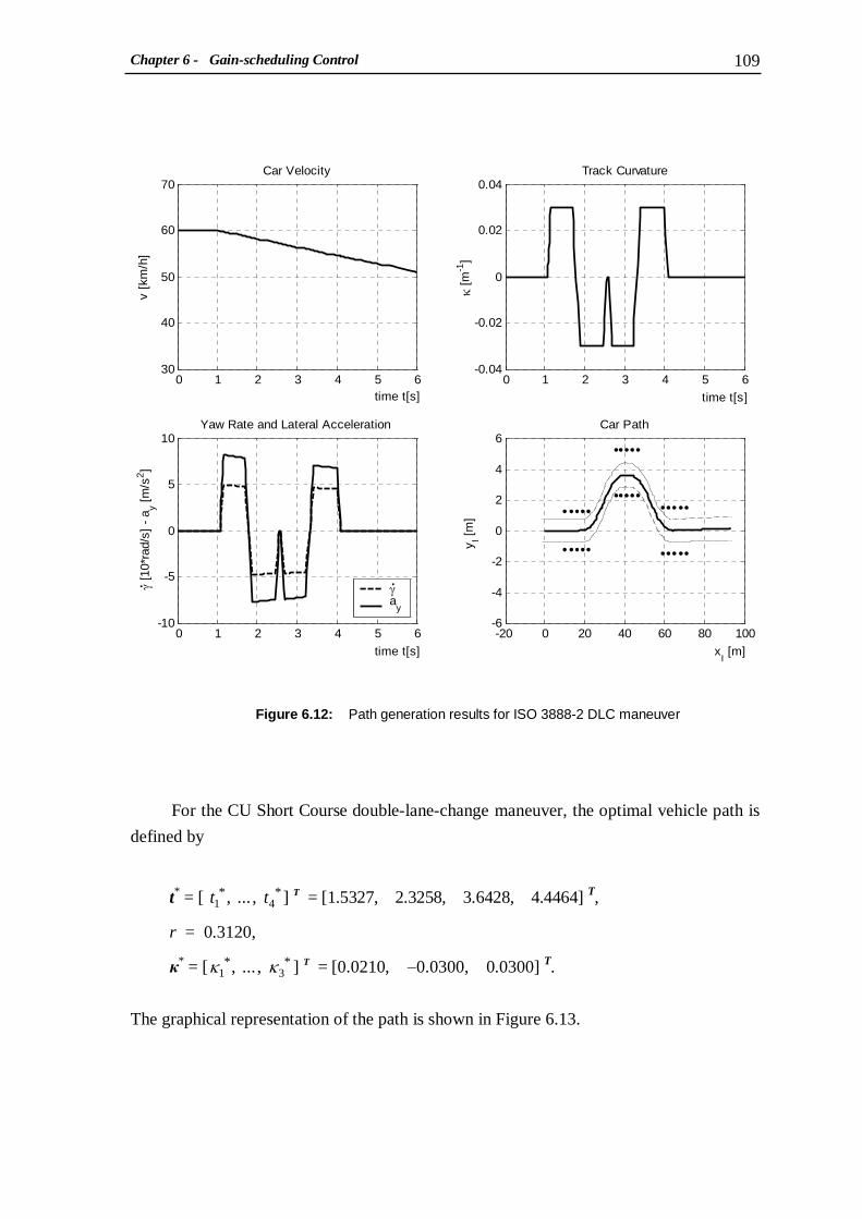
Chapter 6 - Gain-scheduling Control 109
For the CU Short Course double-lane-change maneuver, the optimal vehicle path is
defined by
t* = [ **41 ,..., t t ] T = [1.5327, 2.3258, 3.6428, 4.4464] T,
r = 0.3120,
κ* = [ **31 ,..., κκ ] T = [0.0210, −0.0300, 0.0300] T.
The graphical representation of the path is shown in Figure 6.13.
Figure 6.12: Path generation results for ISO 3888-2 DLC maneuver
0 1 2 3 4 5 6-0.04
-0.02
0
0.02
0.04Track Curvature
time t[s]
κ [m
-1]
0 1 2 3 4 5 630
40
50
60
70Car Velocity
v [k
m/h
]
time t[s]
0 1 2 3 4 5 6-10
-5
0
5
10Yaw Rate and Lateral Acceleration
time t[s]
γ [1
0*ra
d/s]
- a
y [m
/s2]
γa
y
-20 0 20 40 60 80 100-6
-4
-2
0
2
4
6Car Path
xI [m]
y I [m
]
. .

Chapter 6 - Gain-scheduling Control 110
6.3.3 Simulation results with gain-scheduling control
The optimal path parameters obtained from the path generation problem are used for
simulating the studied car in the double-lane-change (DLC) maneuvers with the designed
gain-scheduling control. It should be noted that the spatial car model in this case takes on
the form of a linear-parameter varying system expressed by (3.76) due to the variation of
the car speed and yaw rate during the test.
Figure 6.13: Path generation results for CU Short Course DLC maneuver
0 1 2 3 4 5 6 7-0.04
-0.02
0
0.02
0.04Track Curvature
time t[s]
κ [m
-1]
0 1 2 3 4 5 6 730
40
50
60
70Car Velocity
v [k
m/h
]
time t[s]
0 1 2 3 4 5 6 7-10
-5
0
5
10Yaw Rate and Lateral Acceleration
time t[s]
γ [1
0*ra
d/s]
- a
y [m
/s2]
γa
y
-20 0 20 40 60 80 100 120-6
-4
-2
0
2
4
6Car Path
xI [m]
y I [m
]
. .
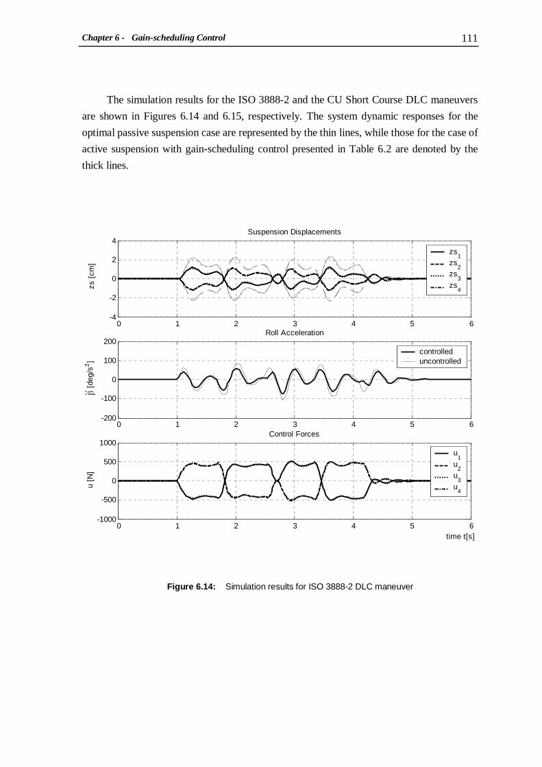
Chapter 6 - Gain-scheduling Control 111
The simulation results for the ISO 3888-2 and the CU Short Course DLC maneuvers
are shown in Figures 6.14 and 6.15, respectively. The system dynamic responses for the
optimal passive suspension case are represented by the thin lines, while those for the case of
active suspension with gain-scheduling control presented in Table 6.2 are denoted by the
thick lines.
Figure 6.14: Simulation results for ISO 3888-2 DLC maneuver
0 1 2 3 4 5 6-4
-2
0
2
4Suspension Displacements
zs [
cm]
zs1
zs2
zs3
zs4
0 1 2 3 4 5 6-200
-100
0
100
200Roll Acceleration
β [de
g/s2
]
controlleduncontrolled
0 1 2 3 4 5 6-1000
-500
0
500
1000Control Forces
time t[s]
u [N
]
u1
u2
u3
u4
..

Chapter 6 - Gain-scheduling Control 112
As can be seen clearly from the figures, the suspension displacements zSi and car body roll
acceleration β&& for both double-lane-change maneuvers are significantly reduced by the
action of the controlled forces based on the designed parameter-dependent controller.
Compared to the case of passive suspension, the active suspension improves the car ride
safety by about 47% for the ISO 3888-2 and 52% for the CU Short Course DLC maneuver.
At the same time the car ride comfort criterion value reduces by 31% and 38%,
respectively. The improvement in the ride comfort criterion of the car can be explained by
the optimization results shown in Figure 5.9 where both ride safety and ride comfort criteria
tend to lower left corner even when optimizing ride safety only. The obtained results above
demonstrate obviously the effectiveness of active suspensions with gain-scheduling control
on both ride safety and ride comfort criteria for passenger cars in yaw motion.
0 1 2 3 4 5 6 7-4
-2
0
2
4Suspension Displacements
zs [
cm]
zs1
zs2
zs3
zs4
0 1 2 3 4 5 6 7-200
-100
0
100
200Roll Acceleration
β [de
g/s2
]
controlleduncontrolled
0 1 2 3 4 5 6 7-1000
-500
0
500
1000Control Forces
time t[s]
u [N
]
u1
u2
u3
u4
..
Figure 6.15: Simulation results for CU Short Course DLC maneuver
Chapter 7 - Summary 113
Chapter 7
Summary
Aiming to design optimal controllers for passenger cars with active suspensions,
optimization methods are applied to various investigations in this dissertation. The
obtained results show that both ride safety and ride comfort of the car in yaw motion are
improved significantly with the designed controllers. The effectiveness of active
suspensions on the vehicle lateral dynamics is demonstrated based on a simplified and
linearized three-degree-of-freedom spatial car model featuring handling performance,
where the effects of suspension geometry are taken into account.
Since all states and disturbances of the spatial car model are assumed to be available
from online measurements, the linear quadratic regulator (LQR) algorithm is applied to
define the optimal control law. The LQR control theory is introduced for linear systems
without disturbances, and then extended to linear systems with measurable disturbances
resulting in an optimal control law with state-feedback and disturbance-feed forward
controller. The application of the LQR control on the spatial car model shows the
usefulness of this approach since the optimal controllers with a large number of unknowns
can be easily derived by choosing appropriately a few weighting factors only.
The obtained results also show that optimal solutions might not be found by
choosing the weighting factors by hand if the control problem is subject to constraints on
the states, measured outputs or control inputs. This drawback of the conventional method
of designing the LQR control is overcome by applying a multi-criterion optimization
approach, where the weighting factors become design variables of the associated MCO
problem. With the combination of the LQR algorithm the number of design variables of
the MCO problem defining the optimal controllers can be reduced significantly. The
MCO problem for the spatial car model with active suspension is solved based on the

Chapter 7 - Summary 114
compromise method and recursive knee approach. Optimization results demonstrate the
effectiveness of the proposed optimization method.
The influences of suspension and tire compliance on vehicle rollover stability are
considered in order to determine the operating region of the studied spatial car model.
Aiming to maintain the desired performances of the system which can be changed due to
the variation in the system parameters, gain-scheduling control design is investigated. The
global parameter-dependent controller results from the two following design steps: first
the local controllers at specified operation points are computed, then the components of
the global controller is interpolated as polynomial functions of the system varying
parameters. The effectiveness of the designed gain-scheduling control is demonstrated by
the simulation of ISO 3882-2 and Consumers Union Short Course double-lane-change
maneuvers, which are designated as the standard handling tests for passenger cars. The
simulation parameters result from a path which minimizes the vehicle lateral dynamics
and is found itself by an optimization problem.
Due to limitation in time, this dissertation cannot focus on all aspects of each
spreading problem, and some future research is desirable. To describe sufficiently the
vehicle lateral dynamics, the effects of tire dynamics on the vehicle vibration and
handling must be included, which were omitted in this research. In addition, although all
states and disturbances of the studied spatial car model are measurable, received signals in
practice are often corrupted by measurement noise, resulting in discontinuous control. To
apply effectively the LQR control, optimal state-feedback and disturbance-feed forward
controller has to be combined with a Kalman optimal estimator. Furthermore, the
achievements of this research should be verified by practical experiments.
Bibliography 115
Bibliography
[1]
[2]
[3]
[4]
[5]
[6]
[7]
[8]
[9]
[10]
[11]
Ackermann, J., Robuste Regelung - Analyse und Entwurf von linearen
Regelungssystemen mit unsicheren physikalischen Parametern. Berlin: Springer, 1993.
Ammon, D., Modellbildung und Systementwicklung in der Fahrzeugdynamik.
Stuttgart: Teubner, 1997.
Andersson, J., Multi-Objective Optimization in Engineering Design. Ph.D. Thesis.
Linköping University, 2001.
Bail, T. R., A Disturbance-Rejection Problem for a 2-D Airfoil. M.Sc. Thesis.
Virginia University, 1997.
Balas, G., Chiang, R., Packard, A. and Safonov, M., Robust Control Toolbox User’s
Guide, Version 3. The Math Works, Inc., 2004.
Balas, G. J., Linear Parameter-Varying Control and Its Application to a Turbofan
Engine. In: International Journal of Robust and Nonlinear Control 12 (2002) 763-796.
Bestle, D., Analyse und Optimierung von Mehrkörpersystemen. Berlin: Springer, 1994.
Bodie, M. O. and Hac, A., Closed Loop Yaw Control of Vehicles Using Magneto-
Rheological Dampers. SAE Transactions 109 (2000) 132-139.
Bruzelius, F., LPV-Based Gain Scheduling. Ph.D. Thesis. Göteborg: Chalmers
University of Technology, 2002.
Chantranuwathana, S. and Peng, H., Adaptive Robust Force Control for Vehicle
Active Suspensions. International Journal of Adaptive Control and Signal Processing
18 (2004) 83-102.
Chen, P. C. and Huang, A. C., Adaptive Multiple-Surface Sliding Control of
Hydraulic Active Suspension Systems Based on the Function Approximation
Technique. Journal of Vibration and Control 11 (2005) 685-706.
Bibliography 116
[12]
[13]
[14]
[15]
[16]
[17]
[18]
[19]
[20]
[21]
[22]
[23]
Chen, W., Sahai, A., Messac, A. and Sundararaj, G. J., Exploration of the
Effectiveness of Physical Programming in Robust Design. ASME Journal of
Mechanical Design 122 (2000) 17-26. Choi, S. B., Lee, H. S. and Park, Y. P., H∞ Control Performance of a Full-Vehicle
Suspension Featuring Magnetorheological Dampers. Vehicle System Dynamics 38
(2002) 341-360. Colaneri, P., Geromel, J. C. and Locatelli, A., Control Theory and Design. London:
Academic Press Limited, 2001.
Coleman, T., Branch, M. A. and Grace, A., Optimization Toolbox User’s Guide,
Version 3. The MathWorks, Inc., 2004.
Collette, Y. and Siarry, P., Multi-Objective Optimization: Principles and Case
Studies. Berlin: Springer, 2003.
Das, I., An Improved Technique for Choosing Parameters for Pareto Surface
Generation Using Normal-Boundary Intersection. In: WCSMO-3 Proceedings,
Buffalo, (1999) 411-413.
Das, I., On Characterizing the ‘Knee’ of the Pareto Curve based on Normal-Boundary
Intersection. Structural and Multidisciplinary Optimization 18 (1999) 107-115. Das, I. and Dennis, J. E., Normal-Boundary Intersection: A New Method for Generating
the Pareto Surface in Nonlinear Multicriteria Optimization Problems. Society for
Industrial and Applied Mathematics 8 (1998) 631-657. Deb, K., Multi-Objective Optimization using Evolutionary Algorithms. Weinheim:
John Wiley & Sons Inc., 2001. Donahue, M. D., Implementation of an Active Suspension, Preview Controller for
Improved Ride Comfort. M. Sc. Thesis. University of California at Berkeley, 2001.
Eberhard, P., Dignath, F. and Kübler, L., Parallel Evolutionary Optimization of
Multibody Systems with Application to Railway Dynamics. Multibody System
Dynamics 9 (2003) 143-164. Eberhard, P., Schiehlen, W. and Bestle, D., Some Advantages of Stochastic Methods
in Multicriteria Optimization of Multibody Systems. Archive of Applied Mechanics
69 (1999) 543-554.
Bibliography 117
[24]
[25]
[26]
[27]
[28]
[29]
[30]
[31]
[32]
[33]
[34]
[35]
Eberhard, P. and Schiehlen, W., Hierarchical Modeling in Multibody Dynamics.
Archive of Applied Mechanics 68 (1998) 237-246.
Fitzpatrick, K. L., Applications of Linear Parameter-Varying Control for Aerospace
Systems. M. Sc. Thesis. University of Florida, 2003.
Forkenbrock, G. J., Elsasser, D. and O’Harra, B., NHTSA’s Light Vehicle Handling
and ESC Effectivness Research Program. URL http://www-nrd.nhtsa.dot.gov/pdf/
nrd-01/esv/ esv19/05-0221-O.pdf, 2005.
Fujiwara, Y. and Adachi, S., Steering Assistance System for Driver Characteristics
using Gain Scheduling Control. URL http://arx.ee.utsunomiya-u.ac.jp/English/
papers/abst2003/ECC2003.pdf, 2003.
Gahinet, P., Nemirovski, A., Laub, A. J. and Chilali, M., LMI Control Toolbox User’s
Guide. Version 1. The MathWorks, Inc., 1995.
Gaspar, P., Szaszi, I. and Bokor, J., Active Suspension Design Using Linear
Parameter Varying Control. International Journal of Vehicle Autonomous Systems 1
(2003) 206-221.
Gärtner, A. and Saeger, M., Simulationsumgebung zur Untersuchung aktiver
Wankstabilisierung in Verbindung mit einer Fahrdynamikregelung. Essen: Simulation
in der Fahrzeugdynamik, 2003.
Genç, S., Synthesis and Properties of Magnetorheological (MR) fluids. Ph. D. Thesis.
University of Pittsburgh, 2002.
Genc, A. U., Linear Parameter Varying Modelling and Robust Control of Variable
Cam Timing Engines. Ph. D. Thesis. University of Cambridge, 2002.
Giua, A., Seatzu, C. and Usai, G., A Mixed Suspension System for a Half-Car Vehicle
Model. Dynamics and Control 10 (2000) 375-397.
Hac, A., Influence of Active Chassis Systems on Vehicle Propensity to Maneuver-
Induced Rollovers. SAE Paper 2002-01-0967, 2002.
Hac, A., Rollover Stability Index Including Effects of Suspension Design. SAE Paper
2002-01-0965, 2002.
Bibliography 118
[36]
[37]
[38]
[39]
[40]
[41]
[42]
[43]
[44]
[45]
[46]
[47]
[48]
Halfmann, C. and Holzmann, H., Adaptive Modelle für die Kraftfahrzeugdynamik.
Berlin: Springer, 2003.
He, Y., Design of Rail Vehicles with Passive and Active Suspensions Using
Multidisciplinary Optimization, Multibody Dynamics, and Genetic Algorithms. Ph. D.
Thesis. University of Waterloo, 2003.
Hong, K., Sohn, H. C., and Hedrick, J. K., Modified Skyhook Control of Semi-Active
Suspensions: A New Model, Gain Scheduling, and Hardware-in-the-Loop Tuning.
ASME Journal of Dynamic Systems, Measurement and Control 124 (2002) 158-167. Hyvärinen, J. P., The Improvement of Full Vehicle Semi-Active Suspension through
Kinematical Model. Ph.D. Thesis. University of Oulu, 2004. Kiencke, U. and Nielsen, L., Automotive Control Systems. Berlin: Springer, 2000.
Kim, I. Y. and Weck, O. L. D., Adaptive Weighted-Sum Method for Bi-Objective
Optimization: Pareto Front Generation. Structural and Multidisciplinary Optimization
29 (2004) 149-158.
Kortüm, W. and Lugner, P., Systemdynamik und Regelung von Fahrzeugen. Berlin:
Springer, 1994. Krüger, W., Integrated Design Process for the Development of Semi-Active Landing
Gears for Transport Aircraft. Ph.D. Thesis. University of Stuttgart, 2000.
Kumar, A., Convex Modeling Techniques for Aircraft Control. M.Sc. Thesis.
Virginia Polytechnic Institute and State University, 2000. Lazic, N., Optimal Vehicle Dynamics - Yaw Rate and Side Slip Angle Control Using
4-Wheel Steering. Ph.D. Thesis. Lund Institute of Technology, 2002.
Lu, G., Huang, J., and Tomizuka, M., Vehicle Lateral Control Under Fault in Front
and/or Rear Sensors. University of California: PATH Research Report, UCB-ITS-PRR-
2003-26, 2003. Marler, R.T. and Arora, J.S., Survey of Multi-Objective Optimization Methods for
Engineering. Structural and Multidisciplinary Optimization 26 (2004) 369-395. Mattson, C. A., Mullur, A. A., and Messac, A., Obtaining a Minimal Representation of
Multi-Objective Design Space. Engineering Optimization 36 (2004) 721-740.

Bibliography 119
[49]
[50]
[51]
[52]
[53]
[54]
[55]
[56]
[57]
[58]
[59]
[60]
[61]
Messac, A., Yahaya, A. I., and Mattson, C. A., The Normalized Normal Constraint
Method for Generating the Pareto Frontier. Structural and Multidisciplinary
Optimization 25 (2003) 86-98. Mitschke, M., Dynamik der Kraftfahrzeuge, Band B: Schwingungen. Berlin:
Springer, 1990. Mitschke, M., Dynamik der Kraftfahrzeuge, Band C: Fahrverhalten. Berlin:
Springer, 1990. Moscinski, J. and Ogonowski, Z., Advanced Control with Matlab and Simulink.
London: Ellis Horwood Limited, 1995. Moylan, P. J. and Moore, J. B., Generalizations of Singular Optimal Control
Theory. London: Pergamon Press, 1971. O’Hara, S. R., Vehicle Path Optimization of Emergency Lane Change Maneuvers
for Vehicle Simulation. M. Sc. Thesis. University of Maryland, 2005. Pang, L., Kamath, G. M., and Wereley, N. M., Analysis and Testing of a Linear
Stroke Magnetorhehological Damper. AIAA/ASME/AHS Adaptive Structures 4
(1998) 2841-2856. Paré, C. A., Experimental Evaluation of Semiactive Magneto-Rheological
Suspensions for Passenger Vehicles. M. Sc. Thesis. Virginia Polytechnic Institute
and State University, 1988.
Park, J. H. and Kim, Y. S., Decentralized Variable Structure Control for Active
Suspensions based on a Full-Car Model. In: Proceedings of the International
Conference on Control Applications, Trieste (1998) 383-387.
Petersen, I., Johansen, T. A., Kalkkuhl, J., and Lüdermann, J., Wheel Slip Control
in ABS Brakes Using Gain Scheduled Constrained LQR. In: Control Systems
Technology 11 (2003) 799-811. Popp, K. and Schiehlen, W., Fahrzeugdynamik. Stuttgart: Teubner, 1993. Rahnejat, H., Multi Body Dynamics – Vehicles, Machines and Mechanisms.
Warrendale: Society of Automotive Engineers, 1998. Ramirez, W. F., Process Control and Identification. San Diego: Academic Press
Inc., 1994.

Bibliography 120
[62]
[63]
[64]
[65]
[66]
[67]
[68]
[69]
[70]
[71]
[72]
[73]
[74]
Rettig, U. and Stryk, O., Optimal and Robust Damping Control for Semi-Active
Vehicle Suspension. In: Proceedings of the Fifth EUROMECH Nonlinear Dynamics
Conference, Eindhoven University of Technology, MS 20-316, 2005.
Rill, G., Vehicle Modelling for Real Time Applications. Journal of the Braz. Soc.
Mechanical Sciences 19 (1997) 192-206.
Rouieh, S. and Titli, A., Design of Active and Semi-Active Automotive Suspension
Using Fuzzy Logic. In: Proceedings of the IFAC World Congress, Sydney (1993)
253-257.
Ryu, J., State and Parameter Estimation for Vehicle Dynamics Control Using GSP.
Ph. D. Thesis. Stanford University, 2004.
Sampson, D. J. M. and Cebon, D., Active Roll Control of Single Unit Heavy Road
Vehicles. Vehicle System Dynamics 40 (2003) 229-270.
Sampson, D. J. M., Active Roll Control of Articulated Heavy Vehicles. Ph.D. Thesis.
University of Cambridge, 2000.
Sastry, S. and Bodson, M., Adaptive Control - Stability, Convergence, and
Robustness. New Jersey: Prentice-Hall, 1989. Schiehlen, W., Technische Dynamik: Eine Einführung in die analytische Mechanik
und ihre technischen Anwendungen. Stuttgart: Teubner, 1986.
Schiehlen, W., Multibody System Dynamics: Roots and Perspectives. Multibody
System Dynamics 1 (1997) 149-188.
Schwarz, H., Theoretische und experimentelle Methoden der Regelungstechnik, Band
12: Optimale Regelung lineare Systeme. Zürich: Bibliographisches Institut AG, 1976.
Shahian, B. and Hassul, M., Control System Design Using Matlab. New Jersey:
Prentice-Hall International, Inc., 2001.
Shen, X. and Peng, H., Analysis of Active Suspension Systems with Hydraulic
Actuators. Proceedings of the IAVSD Conference, Atsugi, 2 (2003) 546-556.
Shukla, P. K. and Deb, K., On Finding Multiple Pareto-Optimal Solutions Using
Classical and Evolutionary Generating Methods. KanGAL Report Number
2005006, Indian Institute of Technology Kanpur, 2005.
Bibliography 121
[75]
[76]
[77]
[78]
[79]
[80]
[81]
[82]
[83]
[84]
[85]
[86]
Siouris, G. M., Optimal Control and Estimation Theory. New York: John Wiley &
Sons, Inc., 1996. Spencer, B. F., Dyke, S. J., Sain, M. K. and Carlson, J. D., Phenomenological
Model of a Magnetorheological Damper. ASCE Journal of Engineering Mechanics
3 (1996) 201-221.
Steinberg, P., Fahrzeugtechnik 1&2. Lecture notes. Brandenburg University of
Technology Cottbus, 2005. Taghirad, H. D. and Esmailzadeh, E., Automobile Passenger Comfort Assured
Through LQG/LQR Active Suspension. Journal of Vibration and Control 4 (1998)
603-618.
Ungoren, A. Y. and Peng, H., An Adaptive Lateral Preview Driver Model. Vehicle
System Dynamics 43 (2005) 245 - 259.
Ungoren, A. Y. and Peng, H., Evaluation of Vehicle Dynamic Control for Rollover
Prevention. International Journal of Automotive Technology 5 (2004) 115-122.
Ungoren, A. Y., Peng, H. and Milot, D. R., Rollover Propensity Evaluation of an
SUV Equipped with a TRW VSC System. SAE Paper 2001-01-0128, 2001.
Valasek, M., Novak, M., Sika, Z. and Vaculın, O., Extended Ground-Hook - New
Concept of Semi-Active Control of Truck’s Suspension. Vehicle System Dynamics 27
(1997) 289-303.
Vaughan, J. E., Active and Semi-Active Control to Counter Vehicle Payload Variation.
M.Sc. Thesis. Georgia Institute of Technology, 2004.
Venhovens, P. J. T. and Nabb, K., Vehicle Dynamics Estimation Using Kalman
Filters. Vehicle System Dynamics 32 (1999) 171-184.
Viano, D. C. and Parenteau, C., Case Study of Vehicle Maneuvers Leading to
Rollovers: Need for a Vehicle Test Simulating Off-Road Excursions, Recovery and
Handling. SAE Paper 2003-01-0169, 2003.
Wachal, A. and Bestle, D., Use of Air Spring Elements for Vibration Insulation. In:
Proceedings of the Fifth EUROMECH Nonlinear Dynamics Conference, Eindhoven
University of Technology, MS 03-295, 2005.

Bibliography 122
[87]
[88]
[89]
[90]
[91]
[92]
[93]
[94]
[95]
[96]
Wallentowitz, H., Vertikal-/Querdynamik von Kraftfahrzeugen. Institut für
Kraftfahrtwesen Aachen, 2000. Wang, J. Y. and Tomizuka, M., Dynamic Analyses and Robust Lateral Control
Design for Automated Lane Guidance of Heavy Vehicles. Asia Journal of Control 2
(2000) 341-369.
Wang, J. Y. and Tomizuka, M., Gain-Scheduled H-infinity Loop-Shaping Control for
Automated Lane Guidance of Tractor-Semitrailer Combination Vehicles. In:
Proceedings of American Control Conference, Chicago (2000) 2033-2037.
Wang, J. Y. and Tomizuka, M., Robust H∞ Lateral Control of Heavy-Duty Vehicles in
Automated Highway System. In: Proceedings of the American Control Conference, San
Diego, 5 (1999) 3671-3675.
Wang, Y., Hartmann, T. S., Schinkel, M. and Hunt, K. J., A New Approach to
Simultaneous Stabilisation with D Stability and Its Application to Control of
Antilock Braking Systems. In: Proceedings of the International Mechanical
Engineering Congress and Exposition, Anaheim (2001) 729-735.
Willumeit, H. P., Modelle und Modellierungsverfahren in der Fahrzeugdynamik.
Stuttgart: Teubner, 1998.
Wu, F., Control of Linear Parameter Varying Systems. Ph.D. Thesis. University of
California at Berkeley, 1995.
Yi K. and Song B. S., Observer Design for Semi-Active Suspension Control. Vehicle
System Dynamics 32 (1999) 129-148.
Yokoyama, M., Hedrick, J. K. and Toyama, S., A Model Following Sliding Mode
Controller for Semi-Active Suspension Systems with MR Dampers. In: Proceedings of
the American Control Conference, Arlington (2001) 2652-2657.
Zhong, Z., Study on Control Algorithms for Semi-Active Suspensions. Research
Report. Cottbus: Brandenburg University of Technology, 2003.

Appendix A 123
Appendix A
Parameters of the Spatial Car Model
This thesis focuses on a spatial car model introduced in Chapter 3. For computations and
simulations, the parameters in Table A.1 are used throughout this dissertation.
parameter notation value unit
1 sprung mass mS 1460.0 kg
2 roll moment of inertia of the sprung mass IX 460.0 kg m2
3 pitch moment of inertia of the sprung mass IY 2460.0 kg m2
4 yaw moment of inertia of the sprung mass IZ 1900.0 kg m2
5 front suspension damping rate bf 1290.0 Ns/m
6 rear suspension damping rate br 1620.0 Ns/m
7 front suspension stiffness kf 19960.0 N/m
8 rear suspension stiffness kr 17500.0 N/m
9 modified front anti-roll bar stiffness rf 19200.0 N/m/rad
10 modified rear anti-roll bar stiffness rr 9600.0 N/m/rad
Table A.1: Parameters of the studied passenger car

Appendix A 124
11 vertical front tire stiffness ktf 175500.0 N/m
12 vertical rear tire stiffness ktr 175500.0 N/m
13 distance from roll axis to the car’s CG hRC 0.2 m
14 height of roll axis above ground hRV 0.3 m
15 half the distance between the front wheels tf 0.761 m
16 half the distance between the rear wheels tr 0.755 m
17 distance from the car’s CG to front axle lf 1.011 m
18 distance from the car’s CG to rear axle lr 1.803 m
19 minimum turning radius Rmin 10.0 m
20 maximum car speed vmax 56 m/s

Appendix B 125
Appendix B
NEWEUL Output File for the Car Model
NEWEUL is a FORTRAN program for computer-aided generation of symbolic equations
of motion of a multi-body system. This program can be applied in various technical fields,
such as vehicle dynamics, robotics, mechanism dynamic analysis, and for any topological
structure of multi-body systems with holonomic or non-holonomic constraints. The
equations of motion of a multi-body system in both nonlinear and linearized forms can be
automatically generated by the formalisms described in Chapter 2. The output file of
NEWEUL presents not only the results, but also the contents of the input file which has to
be provided by the user. In the following, the NEWEUL output file obtained for the three
degree-of-freedom spatial car model is shown.
C> RAEUMLICHES FAHRZEUGMODELL C> C> Tuan-Anh. Nguyen September,2003 C> C>======================================== C> 0 Steuerparameter: 0=holonom, 1=nichtholonom 0 Komprimierungsart(0-6): 0=vollsymbolisch 4 Zahl der Koordinatensysteme 3 Zahl der (Lage-)Freiheitsgrade 3 Zahl der Hilfsvarablen 9 Zahl der linearisierbaren Groessen 0 Zahl der numerischen Groessen 2 Zahl der Vereinfachungen 0 Zahl der Substitutionsvariable /NEGST=2/ C> (Darstellung der Newton-Eulerschen Gleichungen C> im Inertialsystem) C> C> C> LAGEVEKTOR C> ************
Y: ZC Y: BETA Y: ALPHA C> 2 Automatische Ableitung (1: 1/2; 2: P/PP; 0: keine) C> C> C> HILFSVARIABLEN C> ************** C> HV: XV(T) HV: YV(T) HV: GAMMA(T) C> C> C> LINEARISIERUNG C> **************** C> 1 Vollstaendige Linearisierung C> C> C> VEREINFACHUNGEN

Appendix B 126
C> VFV: XVOTOT*cos(GAMMA)+YVOTOT*sin(GAMMA) VFE: AX C> VFV:-XVOTOT*sin(GAMMA)+YVOTOT*cos(GAMMA) VFE: AY C> C>*********************************************** C>*** *** C>*** A u s g a b e b l o c k 1 *** C>*** *** C>*** A l l g e m e i n e A n g a b e n *** C>*** *** C>***********************************************C> C> Lagevektor Y(1)=ZC Y(2)=BETA Y(3)=ALPHA C> C> 1. Ableitung des Lagevektors Y1(1)=ZCP Y1(2)=BETAP Y1(3)=ALPHAP C> C> 2. Ableitung des Lagevektors Y2(1)=ZCPP Y2(2)=BETAPP Y2(3)=ALPHAPP C> C> Hilfsvariable C> XV=XV(T) C> YV=YV(T) C> GAMMA=GAMMA(T) C> C> Linearisierbare Groessen C> ALPHAPP BETAPP ZCPP ALPHAP BETAP ZCP ALPHA BETA ZC C> C> Vereinfachungen C> VFV=XVOTOT*COS(GAMMA)+YVOTOT* SIN(GAMMA) VFE=AX C> VFV=-XVOTOT*SIN(GAMMA)+YVOTOT* COS(GAMMA) VFE=AY C> C>*********************************************** C>*** *** C>*** A u s g a b e b l o c k 1 - E n d e *** C>*** *** C>***********************************************
C> KOORDINATENSYSTEME C> ************************ C> C> Vehicle Fixed Coordinate - Track Motion C> ---------------------------------------------- KOSART: R - Referenzsystem KOSYNA: YA - Namen des Koordinatensystems KOSYNA: I - Namen des Bezugssystems C> C> **** Rotatorischer Teil **** 1 Zahl der Teildrehungen C> 3 Art der Drehung (-3_+5) C> C> Drehwinkel WINK= GAMMA C> C> **** Translatorischer Teil **** 1 Zahl der Teilvektoren C> KOSYNA: I System fuer Teilvektor C> C> Teilvektor R(1)= XV R(2)= YV R(3)= 0 C> C>********************************************C> C> Roll Motion C> --------------------------- KOSART: R - Referenzsystem KOSYNA: RO - Namen des Koordinatensystems KOSYNA: YA - Namen des Bezugssystems C> C> **** Rotatorischer Teil **** 2 Zahl der Teildrehungen C> 2 Art der Drehung (-3_+5) C> C> Drehwinkel WINK = THETA C> 1 Art der Drehung (-3_+5) C> C> Drehwinkel WINK = BETA C> C> **** Translatorischer Teil **** 1 Zahl der Teilvektoren C> KOSYNA: YA System fuer Teilvektor C> C> Teilvektor R(1)= 0 R(2)= 0 R(3)= HRV+ZC C> C> *******************************************

Appendix B 127
C> C> Car Center C> -------------- KOSART: R - Referenzsystem KOSYNA: PI - Namen des Koordinatensystems KOSYNA: RO - Namen des Bezugssystems C> C> **** Rotatorischer Teil **** 1 Zahl der Teildrehungen C> -2 Art der Drehung (-3_+5) C> C> Drehwinkel WINK = THETA C> C> **** Translatorischer Teil **** 1 Zahl der Teilvektoren C> KOSYNA: PI System fuer Teilvektor C> C> Teilvektor R(1)= 0 R(2)= 0 R(3)= HRC C> C> ********************************************** C> C> Car with Pitch Motion C> -------------------------------------- KOSART: S - Starrkörper KOSYNA: CAR - Namen des Koordinatensystems KOSYNA: PI - Namen des Bezugssystems C> C> **** Rotatorischer Teil **** 1 Zahl der Teildrehungen C> 2 Art der Drehung (-3_+5) C> C> Drehwinkel WINK = ALPHA C> C> **** Translatorischer Teil **** 0 Zahl der Teilvektoren C> C>********************************************** C>*** *** C>*** A u s g a b e b l o c k 2 *** C>*** *** C>*** K o o r d i n a t e n s y s t e m e *** C>*** *** C>**********************************************C> C> Drehungsmatrix YA bzgl. Inertialsystem DS1(1,1)=COS(GAMMA) DS1(1,2)=-SIN(GAMMA) DS1(1,3)=0. DS1(2,1)=SIN(GAMMA) DS1(2,2)=COS(GAMMA) DS1(2,3)=0.
DS1(3,1)=0. DS1(3,2)=0. DS1(3,3)=1.
C> Ortsvektor YA bzgl. Inertialsystem DR1(1)=XV DR1(2)=YV DR1(3)=0. C> C> Drehungsmatrix RO bzgl. YA DS2(1,1)=COS(THETA) DS2(1,2)=SIN(THETA)*SIN(BETA) DS2(1,3)=SIN(THETA)*COS(BETA) DS2(2,1)=0. DS2(2,2)=COS(BETA) DS2(2,3)=-SIN(BETA) DS2(3,1)=-SIN(THETA) DS2(3,2)=SIN(BETA)*COS(THETA) DS2(3,3)=COS(THETA)*COS(BETA) C> C> Ortsvektor RO bzgl. YA DR2(1)=0. DR2(2)=0. DR2(3)=HRV+ZC C> C> Drehungsmatrix PI bzgl. RO DS3(1,1)=COS(THETA) DS3(1,2)=0. DS3(1,3)=-SIN(THETA) DS3(2,1)=0. DS3(2,2)=1. DS3(2,3)=0. DS3(3,1)=SIN(THETA) DS3(3,2)=0. DS3(3,3)=COS(THETA) C> C> Ortsvektor PI bzgl. RO DR3(1)=-HRC*SIN(THETA) DR3(2)=0. DR3(3)=HRC*COS(THETA) C> C> Drehungsmatrix CAR bzgl. PI DS4(1,1)=COS(ALPHA) DS4(1,2)=0. DS4(1,3)=SIN(ALPHA) DS4(2,1)=0. DS4(2,2)=1. DS4(2,3)=0. DS4(3,1)=-SIN(ALPHA) DS4(3,2)=0. DS4(3,3)=COS(ALPHA) C> C> Ortsvektor CAR bzgl. PI DR4(1)=0. DR4(2)=0. DR4(3)=0. C> C>********************************************* C>*** *** C>*** A u s g a b e b l o c k 2 - E n d e *** C>*** *** C>*********************************************
Appendix B 128
C>*** A u s g a b e b l o c k 5 *** C>*** *** C> K i n e m a t i s c h e G r o e s s e n Referenzsystem C>*** *** C>********************************************** C> Kinematische Groessen des Referenzsystems YA LTR1(1,1)=0. LTR1(1,2)=0. LTR1(1,3)=0. LTR1(2,1)=0. LTR1(2,2)=0. LTR1(2,3)=0. LTR1(3,1)=0. LTR1(3,2)=0. LTR1(3,3)=0. C> LRR1(1,1)=0. LRR1(1,2)=0. LRR1(1,3)=0. LRR1(2,1)=0. LRR1(2,2)=0. LRR1(2,3)=0. LRR1(3,1)=0. LRR1(3,2)=0. LRR1(3,3)=0. C> AQTR1(1)=AX AQTR1(2)=AY AQTR1(3)=0. C> AQRR1(1)=0. AQRR1(2)=0. AQRR1(3)=GAMMAOTOT C> OR1(1)=0. OR1(2)=0. OR1(3)=GAMMAOT C> C> Kinematische Groessen des Referenzsystems RO LTR2(1,1)=-SIN(THETA) LTR2(1,2)=0. LTR2(1,3)=0. LTR2(2,1)=BETA*COS(THETA) LTR2(2,2)=0. LTR2(2,3)=0. LTR2(3,1)=COS(THETA) LTR2(3,2)=0. LTR2(3,3)=0. C> LRR2(1,1)=0. LRR2(1,2)=1. LRR2(1,3)=0. LRR2(2,1)=0. LRR2(2,2)=0. LRR2(2,3)=0. LRR2(3,1)=0. LRR2(3,2)=0. LRR2(3,3)=0. C> AQTR2(1)=AX*COS(THETA) AQTR2(2)=AX*BETA*SIN(THETA)+AY
AQTR2(3)=AX*SIN(THETA)-AY*BETA C> AQRR2(1)=-GAMMAOTOT*SIN(THETA)
AQRR2(2)=GAMMAOT*BETAP*COS(THETA)+
GAMMAOTOT*BETA*COS(THETA) AQRR2(3)=GAMMAOTOT*COS(THETA) C> OR2(1)=-GAMMAOT*SIN(THETA)+BETAP OR2(2)=GAMMAOT*BETA*COS(THETA) OR2(3)=GAMMAOT*COS(THETA) C> C> Kinematische Groessen des Referenzsystems PI LTR3(1,1)=0. LTR3(1,2)=0. LTR3(1,3)=0. LTR3(2,1)=BETA*COS(THETA) LTR3(2,2)=-HRC*COS(THETA) LTR3(2,3)=0. LTR3(3,1)=1. LTR3(3,2)=0. LTR3(3,3)=0. C> LRR3(1,1)=0. LRR3(1,2)=COS(THETA) LRR3(1,3)=0. LRR3(2,1)=0. LRR3(2,2)=0. LRR3(2,3)=0. LRR3(3,1)=0. LRR3(3,2)=-SIN(THETA) LRR3(3,3)=0. C> AQTR3(1)=-AY*BETA*SIN(THETA)+AX+2.*HRC* GAMMAOT*BETAP*COS(THETA)+ HRC* GAMMAOTOT*BETA*COS(THETA) AQTR3(2)=AX*BETA*SIN(THETA)+AY+ HRC*GAMMAOT**2*BETA*COS(THETA) AQTR3(3)=-AY*BETA*COS(THETA) C> AQRR3(1)=0. AQRR3(2)=GAMMAOT*BETAP*COS(THETA)+ GAMMAOTOT*BETA*COS(THETA) AQRR3(3)=GAMMAOTOT C> OR3(1)=BETAP*COS(THETA) OR3(2)=GAMMAOT*BETA*COS(THETA) OR3(3)=-BETAP*SIN(THETA)+GAMMAOT C> C>********************************************* C>*** *** C>*** A u s g a b e b l o c k 5 - E n d e *** C>*** *** C>*** *** C>********************************************* C>*** A u s g a b e b l o c k 6 *** C>*** *** C>*** K i n e m a t i s c h e G r o e s s e n Koerper C>*** *** C>*** *** C>*********************************************

Appendix B 129
C> Kinematische Groessen des Starrkoerpers CAR C> im Inertialsystem C> LT1(1,1)=0. LT1(1,2)=-HRC*BETA*SIN(THETA)* COS(THETA)*COS(GAMMA)+HRC* SIN(GAMMA)*COS(THETA) LT1(1,3)=0. LT1(2,1)=0. LT1(2,2)=-HRC*BETA*SIN(THETA)* SIN(GAMMA)*COS(THETA)-HRC* COS(THETA)*COS(GAMMA) LT1(2,3)=0. LT1(3,1)=1. LT1(3,2)=-HRC*BETA*COS(THETA)**2 LT1(3,3)=0. C> AQT1(1)=AX*COS(GAMMA)+2.*HRC* GAMMAOT*BETAP*COS(THETA)* COS(GAMMA)+HRC*GAMMAOTOT*BETA* COS(THETA)*COS(GAMMA)- AY*SIN(GAMMA)- HRC*GAMMAOT**2*BETA*SIN(GAMMA)* COS(THETA) AQT1(2)=AX*SIN(GAMMA)+2.*HRC* GAMMAOT*BETAP*SIN(GAMMA)* COS(THETA)+HRC*GAMMAOTOT*BETA* SIN(GAMMA)*COS(THETA)+AY*COS(GAMMA)+ HRC*GAMMAOT**2*BETA*COS(THETA)* COS(GAMMA) AQT1(3)=0. C> LR1(1,1)=0. LR1(1,2)=COS(THETA)*COS(GAMMA) LR1(1,3)=BETA*SIN(THETA)*COS(GAMMA)- SIN(GAMMA) LR1(2,1)=0. LR1(2,2)=SIN(GAMMA)*COS(THETA) LR1(2,3)=BETA*SIN(THETA)*SIN(GAMMA)+ COS(GAMMA) LR1(3,1)=0. LR1(3,2)=-SIN(THETA) LR1(3,3)=BETA*COS(THETA) C> AQR1(1)=-GAMMAOT*ALPHAP*COS(GAMMA)- GAMMAOT*BETAP*SIN(GAMMA)*COS(THETA) AQR1(2)=-GAMMAOT*ALPHAP*SIN(GAMMA)+ GAMMAOT*BETAP*COS(THETA)*COS(GAMMA) AQR1(3)=GAMMAOTOT C> O1(1)=BETAP*COS(THETA)*COS(GAMMA)- ALPHAP*SIN(GAMMA) O1(2)=BETAP*SIN(GAMMA)*COS(THETA)+ ALPHAP*COS(GAMMA) O1(3)=-BETAP*SIN(THETA)+GAMMAOT C> C>********************************************** C>*** *** C>*** A u s g a b e b l o c k 6 - E n d e ***C>*** *** C>*** *** C>**********************************************
C> MASSENGEOMETRISCHE DATEN C> ************************* C> C> Car with Pictch Motion KOSYNA: CAR Namen des Koordinatensystems C> C> Masse Mass = MC C> C> Traegheitstensor KOSYNA: CAR System fuer Angabe der Traegheitstensors C> I(1,1)= IX I(2,1)= 0 I(2,2)= IY I(3,1)= 0 I(3,2)= 0 I(3,3)= IZ C>********************************************* C>*** *** C>*** A u s g a b e b l o c k 7 *** C>*** *** C>*** M a s s e n g e o m e t r i s c h e G r o e s s e n C>*** *** C>*** *** C>********************************************* C> C> Massengeometrische Groessen fuer CAR MA1=MC I1(1,1)=IX*COS(GAMMA)**2+2.*IX*BETA* SIN(THETA)*SIN(GAMMA)*COS(GAMMA)- 2.*IY*BETA*SIN(THETA)*SIN(GAMMA)* COS(GAMMA)+ IY*SIN(GAMMA)**2 I1(2,1)=IX*SIN(GAMMA)*COS(GAMMA)+ IX*BETA*SIN(THETA)*IN(GAMMA)**2- IX*BETA*SIN(THETA)*COS(GAMMA)**2- IY*BETA*SIN(THETA)*SIN(GAMMA)**2+ IY*BETA*SIN(THETA)*COS(GAMMA)**2- IY*SIN(GAMMA)*COS(GAMMA) I1(2,2)=IX*SIN(GAMMA)**2- 2.*IX*BETA* SIN(THETA)*SIN(GAMMA)* COS(GAMMA)+ 2.*IY*BETA*SIN(THETA)*SIN(GAMMA)* COS(GAMMA)+IY*COS(GAMMA)**2 I1(3,1)=-IX*ALPHA*COS(GAMMA)-IY*BETA* SIN(GAMMA)*COS(THETA)+ IZ*ALPHA* COS(GAMMA)+IZ*BETA*SIN(GAMMA)* COS(THETA) I1(3,2)=-IX*ALPHA*SIN(GAMMA)+IY*BETA* COS(THETA)*COS(GAMMA)+IZ*ALPHA* SIN(GAMMA)-IZ*BETA*COS(THETA)* COS(GAMMA) I1(3,3)=IZ C>****** *************************************** C>*** *** C>*** A u s g a b e b l o c k 7 - E n d e *** C>*** *** C>********************************************
Appendix B 130
C> EINGEPRAEGTE KRAEFTE C> ********************** C> C> Applied Force on CAR C> ----------------------------------------------- C> Art der Kraft/des Moments (GK,AK,AM,IK,IM,$END) FLEART: AK C> System auf das die Kraft wirkt KOSYNA: CAR 1.System (Wirkung positiv) C> C> System, in dem die Kraft eingegeben wird KOSYNA: CAR C> C> Kraft/Moment eingeben FLE(1)= 0 FLE(2)= 0 FLE(3)= FZC C> C> Applied Moments on CAR C> ------------------------------------------------- C> Art der Kraft/des Moments (GK,AK,AM,IK,IM,$END) FLEART: AM C> C> System auf das das Moment wirkt KOSYNA: CAR 1.System (Wirkung positiv) C> C> System, in dem das Moment eingegeben wird KOSYNA: CAR C> C> Kraft/Moment eingeben FLE(1)= LBETA FLE(2)= LALPHA FLE(3)= 0 C> C>********************************************** C> FLEART: $END C C>********************************************** C>*** *** C>*** A u s g a b e b l o c k 8 *** C>*** *** C>*** K r a e f t e / M o m e n t e *** C>*** *** C>********************************************** C> C> Kraefte/Momente auf CAR C> im Inertialsystem FE1(1)=FZC*ALPHA*COS(GAMMA)+FZC* BETA*SIN(GAMMA)*COS(THETA) FE1(2)=FZC*ALPHA*SIN(GAMMA)-FZC*BETA* COS(THETA)*COS(GAMMA) FE1(3)=FZC C> LE1(1)=LALPHA*BETA*SIN(THETA)* COS(GAMMA)+LBETA*COS(GAMMA)-
LALPHA*SIN(GAMMA)+LBETA*BETA* SIN(THETA)*SIN(GAMMA)
LE1(2)=LALPHA*BETA*SIN(THETA)* SIN(GAMMA)+LBETA*SIN(GAMMA)+ LALPHA*COS(GAMMA)-LBETA*BETA* SIN(THETA)*COS(GAMMA) LE1(3)=LALPHA*BETA*COS(THETA)- LBETA*ALPHA C> C>********************************************* C>*** *** C>*** A u s g a b e b l o c k 8 - E n d e *** C>*** *** C>*** *** C>********************************************* C>********************************************* C>*** *** C>*** A u s g a b e b l o c k 9 *** C>*** *** C>*** N E W T O N - E U L E R - G l e i c h u n g e n C>*** *** C>*** *** C>********************************************* C> C> Massenmatrix MQT1(1,1)=0. MQT1(1,2)=MC*HRC*SIN(GAMMA)* COS(THETA) MQT1(1,3)=0. MQT1(2,1)=0. MQT1(2,2)=-MC*HRC*COS(THETA)* COS(GAMMA) MQT1(2,3)=0. MQT1(3,1)=MC MQT1(3,2)=0. MQT1(3,3)=0. MQR1(1,1)=0. MQR1(1,2)=IX*COS(THETA)*COS(GAMMA) MQR1(1,3)=-IY*SIN(GAMMA) MQR1(2,1)=0. MQR1(2,2)=IX*SIN(GAMMA)*COS(THETA) MQR1(2,3)=IY*COS(GAMMA) MQR1(3,1)=0. MQR1(3,2)=-IZ*SIN(THETA) MQR1(3,3)=0. C> C> Kreisel-, Zentrifugal- und Corioliskraefte KQT1(1)=MC*AX*COS(GAMMA)+2.*MC* HRC*GAMMAOT*BETAP*COS(THETA)* COS(GAMMA)+MC*HRC*GAMMAOTOT* BETA*COS(THETA)*COS(GAMMA)- MC*AY*SIN(GAMMA)-MC*HRC*GAMMAOT**2* BETA*SIN(GAMMA)*COS(THETA) KQT1(2)=MC*AX*SIN(GAMMA)+2.*MC*HRC* GAMMAOT*BETAP*SIN(GAMMA)* COS(THETA)+MC*HRC*GAMMAOTOT*BETA* SIN(GAMMA)*COS(THETA)+ MC*AY* COS(GAMMA)+MC*HRC*GAMMAOT**2* BETA*COS(THETA)*COS(GAMMA) KQT1(3)=0.
Appendix B 131
KQR1(1)=-IX*GAMMAOTOT*ALPHA* COS(GAMMA)-IY*GAMMAOTOT*BETA* SIN(GAMMA)*COS(THETA)+IZ*GAMMAOTOT* ALPHA*COS(GAMMA)+ IZ*GAMMAOTOT* BETA*SIN(GAMMA)*COS(THETA)- IX*GAMMAOT*ALPHAP*COS(GAMMA)- IY*GAMMAOT*BETAP*SIN(GAMMA)* COS(THETA)+IX*GAMMAOT**2* ALPHA*SIN(GAMMA)-IY*GAMMAOT**2*BETA* COS(THETA)*COS(GAMMA)-IZ* GAMMAOT**2*ALPHA*SIN(GAMMA)+ IZ*GAMMAOT**2*BETA*COS(THETA)* COS(GAMMA)-IX*GAMMAOT*BETAP* SIN(GAMMA)*COS(THETA)- IY*GAMMAOT* ALPHAP*COS(GAMMA)+IZ*GAMMAOT*BETAP* SIN(GAMMA)*COS(THETA)+IZ*GAMMAOT* ALPHAP*COS(GAMMA) KQR1(2)=-IX*GAMMAOTOT*ALPHA* SIN(GAMMA)+IY*GAMMAOTOT*BETA* COS(THETA)*COS(GAMMA)+IZ*GAMMAOTOT* ALPHA*SIN(GAMMA)- IZ*GAMMAOTOT* BETA*COS(THETA)*COS(GAMMA)- IX*GAMMAOT*ALPHAP*SIN(GAMMA)+ IY*GAMMAOT*BETAP*COS(THETA)* COS(GAMMA)-IZ*GAMMAOT*BETAP* COS(THETA)*COS(GAMMA)+ IZ*GAMMAOT*ALPHAP*SIN(GAMMA)- IX*GAMMAOT**2*ALPHA*COS(GAMMA)- IY*GAMMAOT**2*BETA*SIN(GAMMA)* COS(THETA)+ IZ*GAMMAOT**2*ALPHA* COS(GAMMA)+IZ*GAMMAOT**2*BETA* SIN(GAMMA)*COS(THETA)+IX*GAMMAOT* BETAP*COS(THETA)*COS(GAMMA)- IY*GAMMAOT*ALPHAP*SIN(GAMMA) KQR1(3)=IZ*GAMMAOTOT C> C> Eingepraegte Kraefte/Momente QEQT1(1)=FZC*ALPHA*COS(GAMMA)+ FZC*BETA*SIN(GAMMA)*COS(THETA) QEQT1(2)=FZC*ALPHA*SIN(GAMMA)- FZC*BETA*COS(THETA)*COS(GAMMA) QEQT1(3)=FZC QEQR1(1)=LALPHA*BETA*SIN(THETA)* COS(GAMMA)+LBETA*COS(GAMMA)- LALPHA*SIN(GAMMA)+LBETA*BETA* SIN(THETA)*SIN(GAMMA) QEQR1(2)=LALPHA*BETA*SIN(THETA)* SIN(GAMMA)+LBETA*SIN(GAMMA)+ LALPHA*COS(GAMMA)-LBETA*BETA* SIN(THETA)*COS(GAMMA) QEQR1(3)=LALPHA*BETA*COS(THETA)- LBETA*ALPHA C> C>********************************************* C>*** *** C>*** A u s g a b e b l o c k 9 - E n d e *** C>*** *** C>*** *** C>*********************************************
C>******************************************** C>*** *** C>*** A u s g a b e b l o c k 10 *** C>*** *** C>*** B e w e g u n g s - G l e i c h u n g e n *** C>*** *** C>*** *** C>********************************************* C> C> Massenmatrix M(1,1)=MC M(2,1)=0. M(2,2)=IZ*SIN(THETA)**2+MC*HRC**2* COS(THETA)**2+IX*COS(THETA)**2 M(3,1)=0. M(3,2)=0. M(3,3)=IY C> C> Verallgemeinerte Kreisel-, Zentrifugal- und Corioliskraefte K(1)=0. K(2)=-IZ*GAMMAOTOT*SIN(THETA)-MC*HRC* AX*BETA*SIN(THETA)*COS(THETA)-MC*HRC* AY*COS(THETA)-MC*HRC**2*GAMMAOT**2* BETA*COS(THETA)**2-IX*GAMMAOTOT* ALPHA*COS(THETA)+IZ*GAMMAOTOT* ALPHA*COS(THETA)-IX*GAMMAOT* ALPHAP*COS(THETA)-IY*GAMMAOT**2* BETA*COS(THETA)**2+IZ*GAMMAOT**2* BETA*COS(THETA)**2-IY*GAMMAOT* ALPHAP*COS(THETA)+IZ*GAMMAOT* ALPHAP*COS(THETA) K(3)=IY*GAMMAOTOT*BETA*COS(THETA)+ IY*GAMMAOT*BETAP*COS(THETA)- IZ*GAMMAOT*BETAP*COS(THETA)- IX*GAMMAOT**2*ALPHA+IZ*GAMMAOT**2* ALPHA+IX*GAMMAOT*BETAP*COS(THETA) C> C> Verallgemeinerte eingepraegte Kraefte QE(1)=FZC QE(2)=LBETA*ALPHA*SIN(THETA)+LBETA* COS(THETA) QE(3)=LALPHA C> C> Matrix der geschwindigkeitsproportionalen Kraefte P(1,1)=0. P(1,2)=0. P(1,3)=0. P(2,1)=0. P(2,2)=0. P(2,3)=-IX*GAMMAOT*COS(THETA)- IY*GAMMAOT*COS(THETA)+IZ*GAMMAOT* COS(THETA) P(3,1)=0. P(3,2)=IY*GAMMAOT*COS(THETA)- IZ*GAMMAOT*COS(THETA)+IX*GAMMAOT* COS(THETA) P(3,3)=0. C>
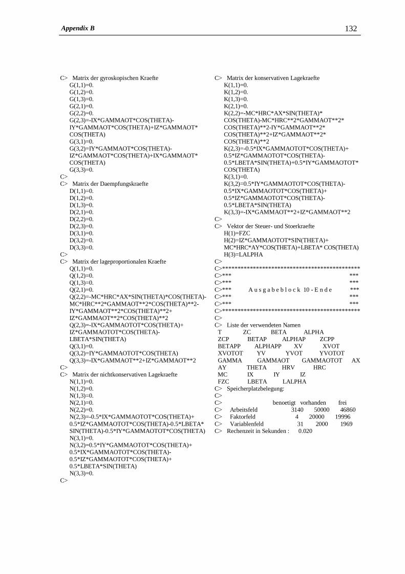
Appendix B 132
C> Matrix der gyroskopischen Kraefte G(1,1)=0. G(1,2)=0. G(1,3)=0. G(2,1)=0. G(2,2)=0. G(2,3)=-IX*GAMMAOT*COS(THETA)- IY*GAMMAOT*COS(THETA)+IZ*GAMMAOT* COS(THETA) G(3,1)=0. G(3,2)=IY*GAMMAOT*COS(THETA)- IZ*GAMMAOT*COS(THETA)+IX*GAMMAOT* COS(THETA) G(3,3)=0. C> C> Matrix der Daempfungskraefte D(1,1)=0. D(1,2)=0. D(1,3)=0. D(2,1)=0. D(2,2)=0. D(2,3)=0. D(3,1)=0. D(3,2)=0. D(3,3)=0. C> C> Matrix der lageproportionalen Kraefte Q(1,1)=0. Q(1,2)=0. Q(1,3)=0. Q(2,1)=0. Q(2,2)=-MC*HRC*AX*SIN(THETA)*COS(THETA)- MC*HRC**2*GAMMAOT**2*COS(THETA)**2- IY*GAMMAOT**2*COS(THETA)**2+ IZ*GAMMAOT**2*COS(THETA)**2 Q(2,3)=-IX*GAMMAOTOT*COS(THETA)+ IZ*GAMMAOTOT*COS(THETA)- LBETA*SIN(THETA) Q(3,1)=0. Q(3,2)=IY*GAMMAOTOT*COS(THETA) Q(3,3)=-IX*GAMMAOT**2+IZ*GAMMAOT**2 C> C> Matrix der nichtkonservativen Lagekraefte N(1,1)=0. N(1,2)=0. N(1,3)=0. N(2,1)=0. N(2,2)=0. N(2,3)=-0.5*IX*GAMMAOTOT*COS(THETA)+ 0.5*IZ*GAMMAOTOT*COS(THETA)-0.5*LBETA* SIN(THETA)-0.5*IY*GAMMAOTOT*COS(THETA) N(3,1)=0. N(3,2)=0.5*IY*GAMMAOTOT*COS(THETA)+ 0.5*IX*GAMMAOTOT*COS(THETA)- 0.5*IZ*GAMMAOTOT*COS(THETA)+ 0.5*LBETA*SIN(THETA) N(3,3)=0. C>
C> Matrix der konservativen Lagekraefte K(1,1)=0. K(1,2)=0. K(1,3)=0. K(2,1)=0. K(2,2)=-MC*HRC*AX*SIN(THETA)* COS(THETA)-MC*HRC**2*GAMMAOT**2* COS(THETA)**2-IY*GAMMAOT**2* COS(THETA)**2+IZ*GAMMAOT**2* COS(THETA)**2 K(2,3)=-0.5*IX*GAMMAOTOT*COS(THETA)+ 0.5*IZ*GAMMAOTOT*COS(THETA)- 0.5*LBETA*SIN(THETA)+0.5*IY*GAMMAOTOT* COS(THETA) K(3,1)=0. K(3,2)=0.5*IY*GAMMAOTOT*COS(THETA)- 0.5*IX*GAMMAOTOT*COS(THETA)+ 0.5*IZ*GAMMAOTOT*COS(THETA)- 0.5*LBETA*SIN(THETA) K(3,3)=-IX*GAMMAOT**2+IZ*GAMMAOT**2 C> C> Vektor der Steuer- und Stoerkraefte H(1)=FZC H(2)=IZ*GAMMAOTOT*SIN(THETA)+ MC*HRC*AY*COS(THETA)+LBETA* COS(THETA) H(3)=LALPHA C> C>*********************************************C>*** *** C>*** *** C>*** A u s g a b e b l o c k 10 - E n d e *** C>*** *** C>*** *** C>*********************************************C> C> Liste der verwendeten Namen T ZC BETA ALPHA ZCP BETAP ALPHAP ZCPP BETAPP ALPHAPP XV XVOT XVOTOT YV YVOT YVOTOT GAMMA GAMMAOT GAMMAOTOT AX AY THETA HRV HRC MC IX IY IZ FZC LBETA LALPHA C> Speicherplatzbelegung: C> C> benoetigt vorhanden frei C> Arbeitsfeld 3140 50000 46860 C> Faktorfeld 4 20000 19996 C> Variablenfeld 31 2000 1969 C> Rechenzeit in Sekunden : 0.020
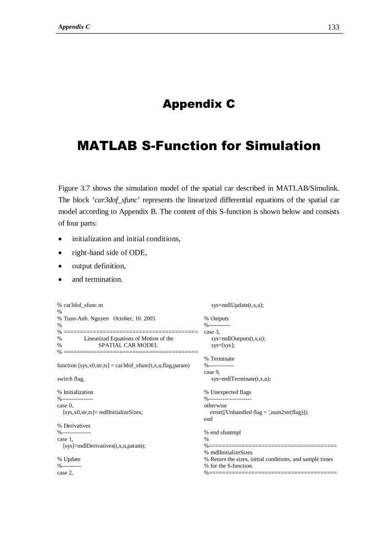
Appendix C 133
Appendix C
MATLAB S-Function for Simulation
Figure 3.7 shows the simulation model of the spatial car described in MATLAB/Simulink.
The block ‘car3dof_sfunc’ represents the linearized differential equations of the spatial car
model according to Appendix B. The content of this S-function is shown below and consists
of four parts:
• initialization and initial conditions,
• right-hand side of ODE,
• output definition,
• and termination. % car3dof_sfunc.m % % Tuan-Anh. Nguyen October, 10. 2005 % % ========================================= % Linearizad Equations of Motion of the % SPATIAL CAR MODEL % ========================================= function [sys,x0,str,ts] = car3dof_sfunc(t,x,u,flag,param) switch flag, % Initialization %---------------- case 0, [sys,x0,str,ts]= mdlInitializeSizes; % Derivatives %--------------- case 1, [sys]=mdlDerivatives(t,x,u,param); % Update %---------- case 2,
sys=mdlUpdate(t,x,u); % Outputs %----------- case 3, sys=mdlOutputs(t,x,u); sys=[sys]; % Terminate %------------- case 9, sys=mdlTerminate(t,x,u); % Unexpected flags %---------------------- otherwise error(['Unhandled flag = ',num2str(flag)]); end % end sfuntmpl % %=======================================% mdlInitializeSizes % Return the sizes, initial conditions, and sample times % for the S-function. %=======================================

Appendix C 134
function [sys,x0,str,ts]=mdlInitializeSizes sizes = simsizes; sizes.NumContStates = 6; sizes.NumDiscStates = 0; sizes.NumOutputs = 6; sizes.NumInputs = 19; sizes.DirFeedthrough = 0; sizes.NumSampleTimes = 1; sys = simsizes(sizes); % initialize the initial conditions x0 = [0 0 0 0 0 0]; % str is always an empty matrix str = []; % initialize the array of sample times ts = [0 0]; % end Initial Conditions %=========================================% mdlDerivatives % Return the derivatives for the continuous states. % LINEARIZED EQUATIONS OF MOTION OF % SPATIAL CAR MODEL % ------------------------------------ % | xp = A*x + B*u + Bw*w | (1) % ------------------------------------ %========================================= function [sys]=mdlDerivatives(t,x,u,param) % reflection of the input to system parameter of NEWEUL % generalized coordinates (Verallgemeine Koordinaten) % ZC = u(1); BETA = u(2); ALPHA = u(3); % generalized velocities (Verallgemeine Geschwindigkeit) % ZCP = u(4); BETAP = u(5); ALPHAP = u(6); % parameters of car motion % XVOTOT = u(7); YVOTOT = u(8); GAMMAOTOT= u(9) ; XVOT = u(10); YVOT = u(11); GAMMAOT = u(12); XV = u(13); YV = u(14);
GAMMA = u(15); % control forces u1 = u(16); u2 = u(17); u3 = u(18); u4 = u(19); u = [u1; u2; u3; u4]; % car accelerations AX = XVOTOT*cos(GAMMA) + … YVOTOT*sin(GAMMA); AY =-XVOTOT*sin(GAMMA) + … YVOTOT*cos(GAMMA); % vector of disturbances w = [AY; GAMMAOTOT]; % end of the reflection % % ----------------------------------------------- % PARAMETERS OF CAR MODEL % ----------------------------------------------- % car parameters % ------------------ THETA = 15/180*pi; HRC = 0.2; % distance of the sprung mass c.g. from % the roll axes HRV = 0.3; % height of the roll axes MC = 1460; % sprung mass IX = 460; % roll moment of inertia of the sprung % mass IY = 2460; % pitch moment of inertia of the sprung % mass IZ = 1900; % yaw moment of inertia of the sprung % mass bf = 1290; % front suspension damping rate br = 1620; % rear suspension damping rate kf = 19960; % front suspension stiffness kr = 17500; % rear suspension stiffness rf = 19200; % modified front anti-roll bar stiffness rr = 9600; % modified rear anti-roll bar stiffness tf = 0.761; % half the distance between the front % wheels tr = 0.755; % half the distance between the rear % wheels lf = 1.011; % distance between the c.g. and the front % axle lr = 1.803; % distance between the c.g. and the rear % axle % % suspension stiffness and damping matrices % -----------------------------------------------------
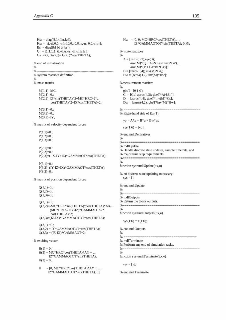
Appendix C 135
Kss = diag([kf,kf,kr,kr]); Ksr = [rf,-rf,0,0; -rf,rf,0,0,; 0,0,rr,-rr; 0,0,-rr,rr]; Bs = diag([bf bf br br]); G = [1,1,1,1; tf,-tf,tr,-tr; -lf,-lf,lr,lr]; Gs = G; Gs(2,:)= G(2,:)*cos(THETA); % end of initialization % % ------------------------------------------------------------------- % system matrices definition % % mass matrix M(1,1)=MC; M(2,1)=0.; M(2,2)=IZ*sin(THETA)^2+MC*HRC^2*… cos(THETA)^2+IX*cos(THETA)^2; M(3,1)=0.; M(3,2)=0.; M(3,3)=IY; % matrix of velocity dependent forces P(1,1)=0.; P(1,2)=0.; P(1,3)=0.; P(2,1)=0.; P(2,2)=0.; P(2,3)=(-IX-IY+IZ)*GAMMAOT*cos(THETA); P(3,1)=0.; P(3,2)=(IY-IZ+IX)*GAMMAOT*cos(THETA); P(3,3)=0.; % matrix of position dependent forces Q(1,1)=0.; Q(1,2)=0.; Q(1,3)=0.; Q(2,1)=0.; Q(2,2)=-MC*HRC*sin(THETA)*cos(THETA)*AX-... (MC*HRC^2+IY-IZ)*GAMMAOT^2*… cos(THETA)^2; Q(2,3)=(IZ-IX)*GAMMAOTOT*cos(THETA); Q(3,1) =0.; Q(3,2) = IY*GAMMAOTOT*cos(THETA); Q(3,3) = (IZ-IX)*GAMMAOT^2; % exciting vector H(1) = 0; H(2) = MC*HRC*cos(THETA)*AY + … IZ*GAMMAOTOT*sin(THETA); H(3) = 0; H = [0; MC*HRC*cos(THETA)*AY + … IZ*GAMMAOTOT*sin(THETA); 0];
Hw = [0, 0; MC*HRC*cos(THETA),… IZ*GAMMAOTOT*sin(THETA); 0, 0]; % state matrices % A = [zeros(3,3),eye(3); -inv(M)*(Q + Gs*(Kss+Ksr)*Gs'),... -inv(M)*(P + Gs*Bs*Gs')]; B = [zeros(3,4); inv(M)*Gs]; Bw = [zeros(3,2); inv(M)*Hw]; %measurement matrices % gbeT= [0 1 0]; C = [Gs', zeros(4,3); gbeT*A(4:6,:)]; D = [zeros(4,4); gbeT*inv(M)*Gs]; Dw = [zeros(4,2); gbeT*inv(M)*Hw]; % ======================================== % Right-hand side of Eq.(1) yp = A*x + B*u + Bw*w; sys(1:6) = [yp]; % end mdlDerivatives % %======================================== % mdlUpdate % Handle discrete state updates, sample time hits, and % major time step requirements. %========================================% function sys=mdlUpdate(t,x,u) % no discrete state updating necessary! sys = []; % end mdlUpdate % %========================================% mdlOutputs % Return the block outputs. %========================================% function sys=mdlOutputs(t,x,u) sys(1:6) = x(1:6); % end mdlOutputs % % ====================================== % mdlTerminate % Perform any end of simulation tasks. %========================================% function sys=mdlTerminate(t,x,u) sys = [x]; % end mdlTerminate

Appendix D 136
Appendix D
MATLAB.m Files for Optimization
This appendix describes the MATLAB.m files used to solve the multi-criterion
optimization (MCO) problems defined for the spatial car model with passive and active
suspensions introduced in Chapter 5 and the path generation problem for the ISO 3882-2
double-lane-change manuever presented in Chapter 6.
D.1 Suspension Optimization
In Section 5.5 the MCO problem defining the optimal parameters for both passive and active
suspensions of the spatial car model is solved based on the compromise method by using the
MATLAB optimization function ‘fmincon’. Ordinarily, the function ‘fmincon’ requires two
MATLAB.m files: one defines the objective function and the other one defines the nonlinear
constraints. The corresponding MATLAB.m files named ‘pass_act_object.m’ and
‘pass_act_const.m’ are shown below.
% cm_pass_act.m % % Tuan-Anh Nguyen, November 2005 % ========================================= % % Compromise Method with LQR Algorithm % for MCO problem finding optimial % passive-active suspension parameters % % =========================================
function [PM]=cm_pass_act(f1min,f12,N) % f1min inidividual minimum f1 % f12 value f1 at f2min % (f1min & f12 are provided % from individual optimization) % N number of calculation points % call program e.g. % [PM] = cm_pass_act(0.3918,0.5243,19) %------------------------------------------------

Appendix D 137
global vc kappa tsim Gs M P Q Hw f1 f3 tsim = 2.5; % simulation time vc=30/3.6; % car speed kappa = 1/10; % curvature %------------------------------------- % car parameters THETA = 15/180*pi; % slope angle of roll axis HRC = 0.2; % distance of the sprung mass c.g. from % the roll axes HRV= 0.3; % height of the roll axes MC = 1460; % sprung mass IX = 460; % roll moment of inertia of the % sprung mass IY = 2460; % pitch moment of inertia of the % sprung mass IZ = 1900; % yaw moment of inertia of the % sprung mass tf = 0.761; % half the distance between the front wheel tr = 0.755; % half the distance between the rear wheel lf = 1.011; % distance between the c.g. and the front axle lr = 1.803; % distance between the c.g. and the rear axle G = [1,1,1,1; tf,-tf,tr,-tr; -lf,-lf,lr,lr]; Gs = G; Gs(2,:)= G(2,:)*cos(THETA); %------------------------------------------------ GAMMAOT = vc*kappa; GAMMAOTOT = 0; AX=0; % mass matrix (massenmatrix) M(1,1)=MC; M(2,1)=0.; M(2,2)=IZ*sin(THETA)^2+MC*HRC^2*... cos(THETA)^2+IX*cos(THETA)^2; M(3,1)=0.; M(3,2)=0.; M(3,3)=IY; % matrix of velocity dependent forces P(1,1)=0.; P(1,2)=0.; P(1,3)=0.; P(2,1)=0.; P(2,2)=0.; P(2,3)=(-IX-IY+IZ)*GAMMAOT*cos(THETA); P(3,1)=0.; P(3,2)=(IY-IZ+IX)*GAMMAOT*cos(THETA); P(3,3)=0.; % matrix of position dependent forces Q(1,1)=0.; Q(1,2)=0.; Q(1,3)=0.; Q(2,1)=0.; Q(2,2)=-MC*HRC*sin(THETA)*cos(THETA)*AX-... (MC*HRC^2+IY-IZ)*GAMMAOT^2*… cos(THETA)^2; Q(2,3)=(IZ-IX)*GAMMAOTOT*cos(THETA);
Q(3,1)=0.; Q(3,2)= IY*GAMMAOTOT*cos(THETA); Q(3,3) = (IZ-IX)*GAMMAOT^2; % disturbance vertor Hw = [0; MC*HRC*cos(THETA); 0]; %------------------------------------------------------------------- % Compromise method with LQR algorithm % ------------------------------------------------------------------ % standard options for optimization with fmincon OPTIONS = optimset('fmincon'); OPTIONS = optimset(OPTIONS,'TolX',1e-6,… 'TolFun',1e-3, 'TolCon',1e-3,... 'DiffMinChange',1e-9,… 'DiffMaxChange',1e-3,... 'LargeScale','off',… 'MaxFunEvals',1e3); %initail design p0 = [1500, 1500, 20000, 20000, 20000, 10000,… 2e7 1e3 1e-2]; % p(1): front suspension damping rate % p(2): rear suspension damping rate % p(3): front suspension stiffness % p(4): rear suspension stiffness % p(5): front anti-roll bar stiffness % p(6): rear anti-roll bar stiffness % p(7): w1 weighting factor on f1 % p(8): w2 weighting factor on f2 % p(9): w3 weighting factor on f3 %lower and upper bounds plb = [1000, 1000, 15000, 15000, 15000, 5000,… 0 0 1e-6]; pub = [2000, 2000, 25000, 25000, 25000, 15000,… 1e8 1e6 1e-2]; %optimization algorithm global mui_f % changing step of constraint bounds % step changing for constraint bounds delta_f1 = (f12-f1min)/N; i = 1; % set changing constraint bounds for mui_f = f1min + N*delta_f1 :-delta_f1 : f1min; Z = clock; % calculation time [p,f,exitflag,output] = fmincon(@pass_act_object,… p0,[],[],[],[],plb,pub,... @pass_act_const,OPTIONS,… f1min,f12,N) if exitflag == -1 break % stop program if no solution is found else

Appendix D 138
% outputs MCO_p(i,:)= p; MCO_f2(i) = f; MCO_f3(i) = f3; MCO_f1(i) = f1; PM(i,:)=[MCO_f1(i)',MCO_f2(i)',… MCO_f3(i)',MCO_p(i,:)]; figure(1); xlabel('ride safety f_1 [cm]'); ylabel('ride comfort f_2 [deg/s^2]'); title('Criterion Space f_1 - f_2'); plot(PM(:,1),PM(:,2), 'b.'); hold on; plot(PM(i,1),PM(i,2), 'ro'); hold on; grid; % new start point p0=p; i = i+1; end end disp(['Calculation time t = ' num2str(etime(clock,Z))... ' s = ' num2str(etime(clock,Z)/60) ' min. ']) %======================================== % % Objective function definition % for cm_pass_act(f1min,f12,N) % %======================================== function [f] = pass_act_object(p,f1min,f12,N) disp(['-------------------------------']) disp(['p =',' ',num2str(p)]) global vc kappa tsim Gs M P Q Hw f1 f3 global h g mui_f % design variables % -------------------- bf = p(1); br = p(2); kf = p(3); kr = p(4); rf = p(5); rr = p(6); Bs = diag([bf bf br br]); Kss = diag([kf,kf,kr,kr]); Ksr = [rf,-rf,0,0; -rf,rf,0,0,; 0,0,rr,-rr; 0,0,-rr,rr]; % system matrices A = [zeros(3,3),eye(3); -inv(M)*(Q + Gs*(Kss+Ksr)*Gs'),... -inv(M)*(P + Gs*Bs*Gs')]; B = [zeros(3,4); inv(M)*Gs]; Bw = [zeros(3,1); inv(M)*Hw];
% measurement matrices gbeT= [0 1 0]; C = [Gs', zeros(4,3); gbeT*A(4:6,:)]; D = [zeros(4,4); gbeT*inv(M)*Gs]; Dw = [zeros(4,1); gbeT*inv(M)*Hw]; % LQR algorithm % ------------------ SYS = ss(A,B,C,D); % weighting matrices Qy = diag([p(7), p(7), p(7), p(7), p(8)]); Ry = diag([p(9), p(9), p(9), p(9)]); % optimal gain matrices K1& K2 [Kx,Px,E]=lqry(SYS,Qy,Ry); R =D'*Qy*D+Ry; Nuw=Dw'*Qy*D; Nxw=C'*Qy*Dw; Kw=(R)\[Nuw'+B'*inv(A'+Kx'*B')*… (Kx'*Nuw'-Nxw-Px*Bw)]; % simulation options my_opt = simset('Initialstep', 0.01,… 'SrcWorkspace', 'current'); % call simulation sim('cm_pass_act_model',tsim, my_opt); % criteria definition f1 = sqrt(sum(J_zs)/length(J_zs)); % ride safety f2 = sqrt(sum(J_bepp)/length(J_bepp)); % ride comfort f3 = sqrt(sum(J_u)/length(J_u)); % control effort % objective function f = f2; disp(['=== ','f1 = ',num2str(f1),' === ',... 'f2 = ',num2str(f2),' === ','f3 = ',num2str(f3)]) disp(['mui_f =',' ',num2str(mui_f)]) % nonlinear constraints h(1) = f1 - mui_f; h(2) = max(max(abs(ui)))-500; g=[]; % no equality constraint %======================================== % % Nonlinear constraints definition % for cm_pass_act(f1min,f12,N) % %======================================== function [h,g] = pass_act_const(p,f1min,f12,N) global h g % see pass_act_object(p,f1min,f12,N) % for constraint computation

Appendix D 139
D.2 Path Generation for Double-Lane-Change Manuever
The following MATLAB.m file is used to solve the path generation problem for the ISO-
3882-2 double-lane-change maneuver presented in Section 6.3.2. The entrance speed of the
car is assumed as v = 60 km/h reducing steadily with a rate rate_v = – 0.5 m/s2. The path is
defined based on 11 parameters: the time points of changing curvature t1 − t6, the rates of
curvature change (assumed to be the same) and the curvatures κ1 − κ 4. The constraints for the
problem are defined based on the positions of the four wheels during simulation and the
wheel track boundaries given in Table 6.3.
% Elk_test_optim.m % % Tuan-Anh Nguyen, Apr. 2006 %========================================= % % Path generation for ISO Doubl_Lane_Change Manuever % (Elk Test) % % ======================================== function [PE]= Elk_test_optim % call program % [PE]=Elk_test_optim %--------------------------- % simulation parameters % -------------------------- v = 60/3.6; % entrance car speed rate_v = -0.5; % reduction rate of car speed tsim = 6; % simulation time global tsim v rate_v poff pskal % initial design p0 = [ 1.05, 1.68, 2.45, 2.60, 3.20, 4.00,... 0.3000,... 0.0300, -0.0300, -0.0300, 0.0300]'; % bounds on design variables kap_max = 9.81/v^2; % from sideway slipping condition plb = [ 0.5 1.0 1.5 2.0 3.0 3.5,... 0.1000,... 0.01 -kap_max -kap_max 0.01]'; pub = [1.5 2.0 2.5 3.0 4.0 4.5,... 0.3145,... kap_max -0.01 -0.01 kap_max]'; % scalarization for optimizing on [0 1] pskal= 1./(pub-plb); % scalarization factor
poff = plb; % offset x_lb = pskal.*(plb-poff); % lower bound x_ub = pskal.*(pub-poff); % upper bound x0 = pskal.*(p0-poff); % start point % standard options for optimization with fminimax OPTIONS = optimset('fminimax'); OPTIONS = optimset(OPTIONS,'TolX',1e-3,… 'TolFun',1e-3,'TolCon',1e-3,... 'DiffMinChange',1e-9,… 'DiffMaxChange',1e-6,... 'LargeScale','off',… 'MaxFunEvals',1e3,'MinAbsMax',4); Z = clock; [x,f,exitflag] = fminimax(@Elk_test_object,x0,… [],[],[],[],x_lb,x_ub,... @Elk_test_const,OPTIONS) % set outputs p=poff+x./pskal; % scalarization turnback PE=p; disp(['Calculation time t = ' num2str(etime(clock,Z))... ' s = ' num2str(etime(clock,Z)/60) ' min. ']) %=======================================% % Objective function definition % for Elk_test_optim % minimize maximum kappa <=> minimize max ay % %======================================= function [f] = Elk_test_object(x) global tsim v rate_v poff pskal global h g p=poff+x./pskal; p=p';

Appendix D 140
disp(['-------------------------------']) disp(['t =',' ',num2str(p(1:6))]) disp(['']) disp(['rate =',' ',num2str(p(7))]) disp(['']) disp(['kappa =',' ',num2str(p(8:11))]) % new design variables for simulation t_1=p(1); t_2=p(2); t_3=p(3); t_4=p(4); t_5=p(5); t_6=p(6); rate_1=p(7); rate_2=-p(7); rate_3=p(7); rate_4=-p(7); rate_5=p(7); rate_6=-p(7); kappa_1=p(8); kappa_2=p(9); kappa_3=p(10); kappa_4=p(11); % simulation option my_opt = simset('Initialstep', 0.01,... 'SrcWorkspace', 'current'); % call simulation [tS,yS]= sim('Elk_test_opt', tsim, my_opt); % objective vector for minmax problem f(1) = abs(kappa_1); f(2) = abs(kappa_2); f(3) = abs(kappa_3); f(4) = abs(kappa_4); % description of the position of test cones for Elch Test %----------------------------------------------------------------- %longitudinal position of cones xc1=[10:12/4:22]; xc2=[(22+13.5):11/4:(35.5+11)]; xc3=[(46.5+12.5):12/4:(59+12)]; xcones=[xc1,xc2,xc3]; % lateral position of upper and lower cones ycu1=[1.25*ones(1,length(xc1))]; ycu2=[5.3*ones(1,length(xc2))]; ycu3=[1.5*ones(1,length(xc3))]; ycl1=[-1.25*ones(1,length(xc1))]; ycl2=[2.25*ones(1,length(xc2))]; ycl3=[-1.5*ones(1,length(xc3))]; yc1 =[ycu1;ycl1]; yc2 =[ycu2;ycl2]; yc3 =[ycu3;ycl3]; ycones=[yc1,yc2,yc3]; % lateral position of wheels % ------------------------------ for i=1:1:4, x=xy_wheel(:,i); % longitudinal position of % wheel ith y=xy_wheel(:,i+4); % lateral position of % wheel ith % section 1 (cone section) [a,k0]=min(abs(xvS-10)); % start of section [a,k1]=min(abs(xvS-22)); % end of section yw1=y(k0:k1);
% section 2 (non-cone section) [a,k2]=min(abs(xvS-35.5)); % section 3 (cone section) [a,k3]=min(abs(xvS-46.5)); yw3=y(k2+1:k3); % section 4 (non-cone section) [a,k4]=min(abs(xvS-59)); % section 5 (cone section) yw5=y(k4+1:end); % nonlinear inequality constraints %--------------------------------------- if mod(i,2)==1 % constraints for left wheels % section 1 h(3*i-2)=max(yw1)-(1.25-0.3); % cone section 3 h(3*i-1)=max(yw3)-(5.30-0.3); % cone section 5 h(3*i)=max(yw5)-(1.5-0.3); elseif mod(i,2)==0 % constraints for right wheels % section 1 h(3*i-2)=-min(yw1)+(-1.25+0.3); % section 3 h(3*i-1)=-min(yw3)+(2.25+0.3); % section 5 h(3*i)=-min(yw5)+(-1.5+0.3); end % if end % for % nonlinear equality constraints %------------------------------------ g = []; % no equality constraint figure(1) title('Car Path'); xlabel('x_I [m]'); ylabel('y_I [m]'); plot (xvS,yvS,'b','LineWidth',1.5);hold on; plot (x3,y3,'g:');hold on; plot (x4,y4,'g:');hold on; plot (x1,y1,'b:');hold on; plot (x2,y2,'b:');hold on; plot (xcones,ycones,'r.','MarkerSize',5); hold off; grid; %======================================= % % Constraint definitions % for Elk_test_optim % % ======================================= function [h,g] = Elk_test_const(x) global h g % see Elk_test_object(x) % for constraint definition