5

XP \1\c.i

APPLICATION OF OLD ELECTRIC LOGSIN THE ANALYSIS OF AUX VASES SANDSTONE(MISSISSIPPIAN) RESERVOIRS IN ILLINOIS

Hannes E. Leetaru

Illinois Petroleum 134

1990

ILLINOIS STATE GEOLOGICAL SURVEYDepartment of Energy and Natural ResourcesMorris W. Leighton, Chief

ILLINOIS GEOLOGICAL

SU.xVE/ LIBRARY

ILLINOIS STATE GEOLOGICAL SURVEY

3 3051 00004 9159

APPLICATION OF OLD ELECTRIC LOGSIN THE ANALYSIS OF AUX VASES SANDSTONE(MISSISSIPPIAN) RESERVOIRS IN ILLINOIS

Hannes E. Leetaru

Illinois Petroleum 134

1990

ILLINOIS STATE GEOLOGICAL SURVEYDepartment of Energy and Natural Resources

Morris W. Leighton, Chief

ILLINOIS GEOLOGICAL

SURVEY LIBRARY

Printed by authority of the State of Illinois/1990/750

CONTENTS

ABBREVIATIONSACKNOWLEDGMENTSABSTRACTINTRODUCTIONBRIEF DESCRIPTION OF OLD ELECTRIC LOGS 4STRATIGRAPHY 5DATA ANALYSIS AND METHODOLOGY RPOROSITY

7Short Normal Method 7Rocky Mountain Method 7Normalized Spontaneous Potential Method 8

PERMEABILITYWATER SATURATIONSUMMARYREFERENCESAPPENDIX

FIGURES1

1

13

15

18

19

21

Generalized upper Valmeyeran and Chesterian geologic column of southern Illinois 1

2 Regional map showing study area and Aux Vases producing fields 23 Principal geologic structures of Illinois 34 Location of wells for which both core and electric logs are available in study area 65 Measured core porosity compared with porosity calculated from the short normal

[Rm taken from the log heading) 76 Measured core porosity compared with porosity calculated from the short normal

(Rm estimated using the Cypress sand) 87 Measured core porosity compared with porosity calculated using

the Rocky Mountain method 88 Electric log of the Cypress and Aux Vases interval showing the sand baseline

and the shale baseline10

9 Electric log of the Cypress and Aux Vases interval showing SP baseline shift 1

1

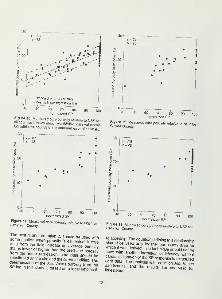
10 Measured core porosity relative to NSP for all counties in study area 121

1

Measured core porosity relative to NSP for Jefferson County 1212 Measured core porosity relative to NSP for Wayne County 1213 Measured core porosity relative to NSP for Hamilton County 1214 Measured core permeability relative to measured core porosity 1315 Measured core permeability relative to NSP for all four counties 1316 Measured core permeability relative to NSP for Jefferson County 1317 Measured core permeability relative to NSP for Wayne County 1418 Measured core permeability relative to NSP for Hamilton County 1419 Pickett plot of estimated porosity relative to apparent FL from the short normal

for King Field, Jefferson County 16

ABBREVIATIONS ACKNOWLEDGMENTS

Fmn

NSP

r

"a

RR~

SPSPSP,

SP.

log

formation factor

cementation exponent

number of wells

normalized spontaneous potential

porosity of the formation

Pearson correlation coefficient

apparent resistivity of the formation

resistivity of the invaded zone

resistivity of the mudresistivity of the mud filtrate

resistivity of the formation 100 percent

saturated with formation water

resistivity of the formation

resistivity of the formation water

spontaneous potential

SP measurement from zone of interest

average SP at the shale baseline

average SP for a clean sandstone

water saturation

This research was done under U.S. Department of

Energy Grant DE-FG22-89BC14250 and the State

of Illinois through Department of Energy and

Natural Resources Grant AE-45. I thank Richard

Howard, Stephen Whitaker, and John Grube of the

ISGS and Daniel Hartmann of DJH Energy

Consulting for their comments and assistance with

this manuscript.

ABSTRACT

Old electric logs (pre-1960) are a valuable sourceof information for the oil industry to use for im-

proved and enhanced oil recovery. In this study,

old electric logs were used effectively to estimate

porosity and water saturation. The empirical

methods described in this report are quick andeasy to use. Results of the analysis can be applied

to identifying passed-over pay in older wells andas input into reservoir models.

Three methods for using old electric logs to esti-

mate the porosity of the Aux Vases Sandstone(Mississippian) were tested for wells in Jefferson,

Wayne, Franklin, and Hamilton Counties in Illinois.

The empirical normalized spontaneous potential

method was significantly better at predicting poros-

ity than were the short normal or Rocky Mountainmethods.

Normalizing spontaneous potential values against

an internal standard can compensate for changesin the scale of the log, the mud resistivity, and the

size of the borehole and allow direct comparisonsof spontaneous potential values between different

drill holes. The clean sandstones within the Cy-press Formation, which occur about 200 feet

above the Aux Vases, were used in this investiga-

tion to normalize (or standardize) the spontaneouspotential.

Although on a regional scale values for permeabili-

ty from the normalized spontaneous potential are

commonly in the correct order of magnitude, theyare not considered accurate enough to use in

reservoir analysis. However, in local areas with

similar diagenetic and depositional facies, the

correlation can be strong enough to allow for

semiquantitative predictions of permeability. Pickett

plot analysis is a viable alternative to the Archieequation in estimating water saturation in the AuxVases. The major advantage of Pickett plot analy-

sis is that neither the cementation exponent nor

the resistivity of the formation water has to beknown to calculate water saturation.

Digitized by the Internet Archive

in 2012 with funding from

University of Illinois Urbana-Champaign

http://archive.org/details/applicationofold134leet

INTRODUCTION

Techniques are presented for using old (generally

pre-1960) electric logs to characterize hydrocarbonreservoirs of the Upper Valmeyeran (Mississippian)

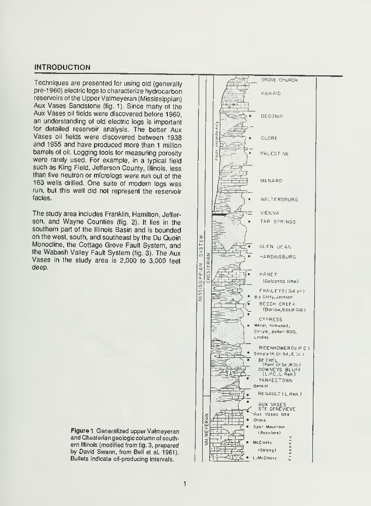
Aux Vases Sandstone (fig. 1). Since many of theAux Vases oil fields were discovered before 1960,an understanding of old electric logs is importantfor detailed reservoir analysis. The better AuxVases oil fields were discovered between 1938and 1955 and have produced more than 1 million

barrels of oil. Logging tools for measuring porosity

were rarely used. For example, in a typical field

such as King Field, Jefferson County, Illinois, less

than five neutron or micrologs were run out of the163 wells drilled. One suite of modern logs wasrun, but this well did not represent the reservoir

facies.

The study area includes Franklin, Hamilton, Jeffer-

son, and Wayne Counties (fig. 2). It lies in thesouthern part of the Illinois Basin and is boundedon the west, south, and southeast by the Du QuoinMonocline, the Cottage Grove Fault System, andthe Wabash Valley Fault System (fig. 3). The AuxVases in the study area is 2,000 to 3,000 feet

deep.

Figure 1 Generalized upper Valmeyeranand Chesterian geologic column of south-

ern Illinois (modified from fig. 3, preparedby David Swann, from Bell et al. 1961).

Bullets indicate oil-producing intervals.

^^

GROVE CHURCH

KINKAID

• DEGONIA

• CLORE

• PALESTINE

MENARD

^

TTD

<1 I "i

~*r.

i.

.i°

i : i.

WALTERSBURG

VIENNA

TAR SPRINGS

GLEN DEAN

HARDINSBURG

HANEY(Golconda lime)

FRAILEYS(Gol.sh)Big Cliffy, Jackson

BEECH CREEK(Barlow, basal Gol.)

CYPRESSWeiler, Kirkwood,

Corlyle,Bellair 900,

Lmdley

RIDENHOWER(U P C )

Sample (P. Cr. Sd., E.III )

BETHEL(Paint CrSd.,W.III.)

DOWNEYS BLUFF(L. PC, U.Ren.)

YANKEETOWNBenoist

RENAULT ( L.Ren.)

AUX VASESSTE GENEVIEVE

"Aux Vases lime

Ohara

Spar Mountain

( Rosiclore)

McClosky co

(Oblong) "°

L. McClosky £

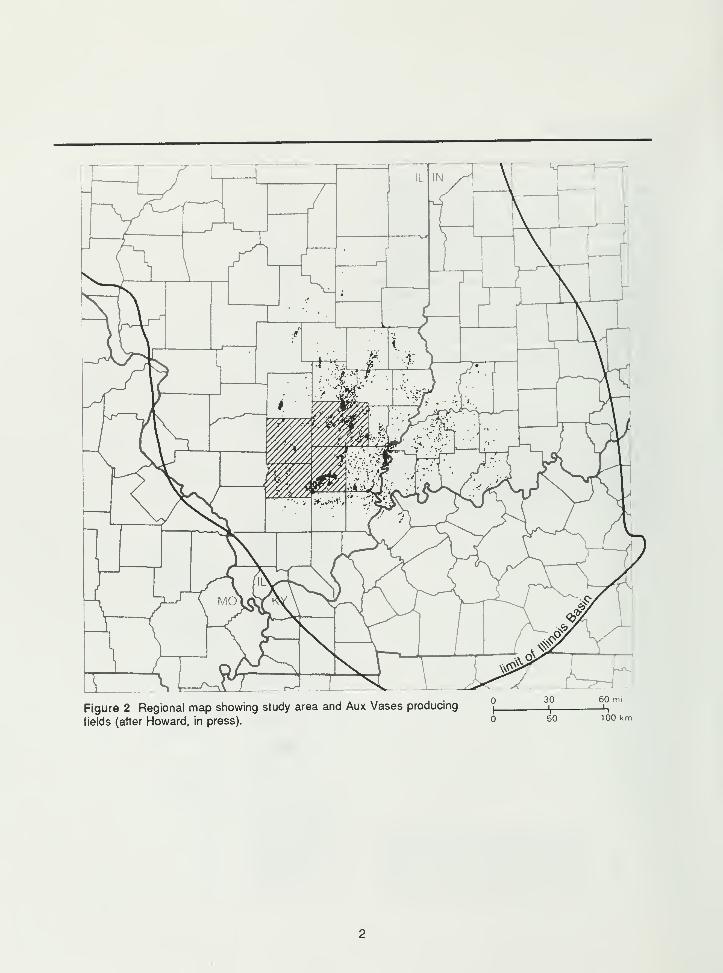
Figure 2 Regional map showing study area and Aux Vases producing

fields (after Howard, in press).-i

—

50

60 mi

—

h

100 km

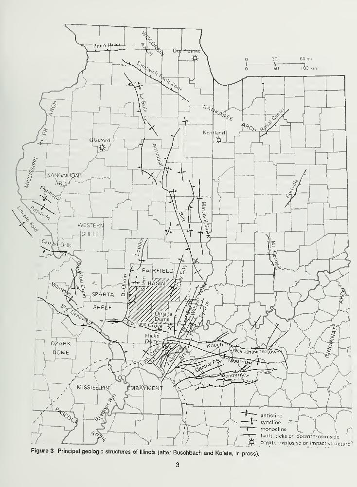
Figure 3 Principal geologic structures of Illinois (after Buschbach and Kolata, in press).

3

BRIEF DESCRIPTION OF OLD ELECTRIC LOGS

Old electric logs are wireline logs that combine the

spontaneous potential (SP) and the normal and

lateral resistivity curves. By 1956, the induction log

began replacing the electric log as the primary

resistivity measurement tool (Hilchie 1979), al-

though in the Illinois Basin, electric logs continued

to be run during the early 1960s.

The SP measures the potential that has developed

opposite a permeable bed in a natural electro-

chemical cell composed of shale, freshwater, and

saltwater (Hilchie 1979). Griffiths (1952) showed

an inverse relationship between the amount of clay

and the magnitude of the SP. The SP-clay relation-

ship is the basis for the technique of estimating

porosity presented in this report. Although the SPmeasures the amount of clay, not porosity and

permeability, an increase in clay implies a corre-

sponding decrease in porosity and permeability.

The normal refers to a log that was introduced by

Schlumberger in 1931 and became the primary

resistivity curve in the early electric log suite

(Hilchie 1979). The type of normal is defined by

the electrode spacing, usually referred to as the

AM spacing, which determines the depth of investi-

gation. In the Illinois Basin, many different elec-

trode spacings were used, of which the most com-

mon were the 16-inch short normal (AM = 16 in.)

and the 64-inch long normal (AM = 64 in.).

The depth of investigation of the normal is as-

sumed to be twice the AM spacing (Hilchie 1979).

At an AM spacing of 16 inches, resistivity is meas-

ured 32 inches from the borehole. At an AMspacing of 64 inches, resistivity is measured 120

inches (-10 feet) from the borehole. The short

normal usually measures the average resistivity of

the invaded zone (R), which is saturated with a

mixture of mud filtrate and original formation fluid.

The long normal measures the apparent resistivity

(Ra ) of the formation. Invasion and thin-bed effects

can still affect the long normal. Simply stated, the

long normal accurately measures formation resis-

tivity if beds are thicker than 1 feet and invasion

is less than 5 feet (Frank 1986).

The lateral, as a resistivity log, is of limited use in

analyzing the Aux Vases Sandstone because beds

must be thicker than 30 feet for the lateral to give

an accurate value for formation resistivity (Rt). The

Aux Vases in the study area is typically less than

30 feet thick and commonly less than 20 feet thick.

The lateral is asymmetrical; it does not peak

opposite the center of the bed, which complicates

interpretation.

STRATIGRAPHY

The Aux Vases Formation is the uppermost unit ofthe Mississippian Valmeyeran Series (fig. 1). TheAux Vases Sandstone in southern Illinois common-ly is fine to medium grained, moderately to well-sorted, and contains 81 to 98 percent quartz andup to 13 percent feldspar (McKay 1980, Weimer et

al. 1982, Young 1983). Calcite, iron oxide, andquartz are the main cementing agents. A typicalreservoir unit consists of a single porous, perme-able lens, with a maximum thickness of 10 to 20feet. Clean porous sandstone reservoirs grade into

silty or calcareous sandstones and shales. In partsof the study area, the Aux Vases contains scat-tered limestone lenses up to 10 feet thick.

Clay minerals have a major effect on log measure-ments. The principal clay mineral groups repre-sented in the Aux Vases are illite, mixed layer(undifferentiated), and chlorite (Smoot 1960,Wilson 1985, Seyler 1988). In addition to decreas-ing the size of the pore throats, clays also increasethe surface area within the pores, thereby increas-

ing the amount of clay-bound (immobile) water.The cation exchange capacity of these clayscauses lower resistivity values and increases thecalculated water saturation values.

The Aux Vases Formation is overlain by thecarbonate-dominated Renault Formation. TheRenault is relatively continuous in the eastern partof the study area (fig. 2), but becomes morediscontinuous and difficult to correlate toward thewestern edge of the study area, where it changesto a sandstone-shale sequence and is indistin-

guishable from the Aux Vases. The resistivity ofthe approximately 1 0-foot-thick carbonate faciesprovides an excellent marker on electric logs.

Underlying the Aux Vases is the Ste. GenevieveFormation, an oolitic or crinoidal limestone with afairly uniform electric log character. The Ste. Gene-vieve can be a good marker that enhances correla-tion, but differentiating the Ste. Genevieve from theAux Vases limestone facies can be difficult.

DATA ANALYSIS AND METHODOLOGY

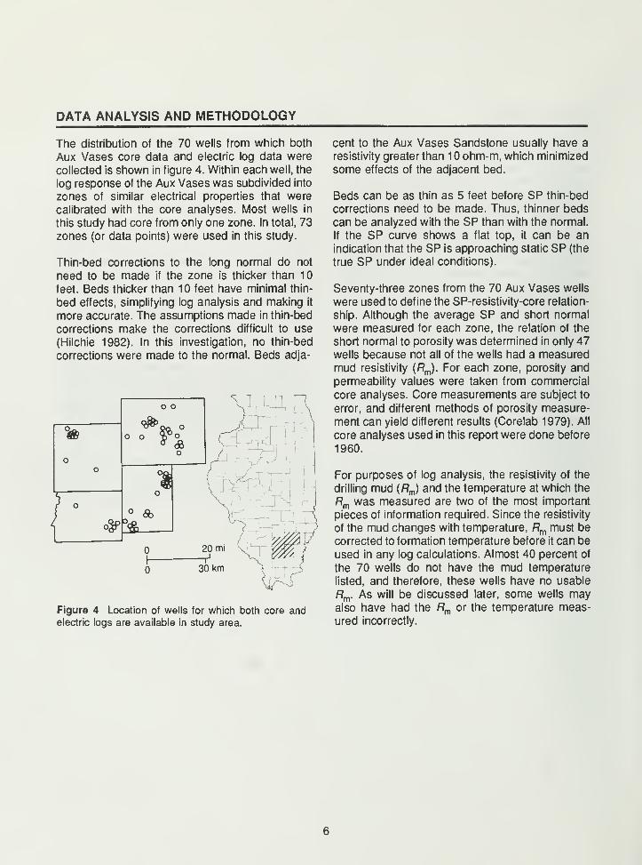
The distribution of the 70 wells from which both

Aux Vases core data and electric log data were

collected is shown in figure 4. Within each well, the

log response of the Aux Vases was subdivided into

zones of similar electrical properties that were

calibrated with the core analyses. Most wells in

this study had core from only one zone. In total, 73

zones (or data points) were used in this study.

Thin-bed corrections to the long normal do not

need to be made if the zone is thicker than 1

feet. Beds thicker than 10 feet have minimal thin-

bed effects, simplifying log analysis and making it

more accurate. The assumptions made in thin-bed

corrections make the corrections difficult to use

(Hilchie 1982). In this investigation, no thin-bed

corrections were made to the normal. Beds adja-

o <3

oo

o o %*o

o

1o

° <5b

I' #I

20

—

r

30

Figure 4 Location of wells for which both core andelectric logs are available in study area.

cent to the Aux Vases Sandstone usually have a

resistivity greater than 10 ohm-m, which minimized

some effects of the adjacent bed.

Beds can be as thin as 5 feet before SP thin-bed

corrections need to be made. Thus, thinner beds

can be analyzed with the SP than with the normal.

If the SP curve shows a flat top, it can be an

indication that the SP is approaching static SP (the

true SP under ideal conditions).

Seventy-three zones from the 70 Aux Vases wells

were used to define the SP-resistivity-core relation-

ship. Although the average SP and short normal

were measured for each zone, the relation of the

short normal to porosity was determined in only 47wells because not all of the wells had a measuredmud resistivity (Rm ). For each zone, porosity and

permeability values were taken from commercial

core analyses. Core measurements are subject to

error, and different methods of porosity measure-

ment can yield different results (Corelab 1979). All

core analyses used in this report were done before

1960.

For purposes of log analysis, the resistivity of the

drilling mud (F?m ) and the temperature at which the

Rm was measured are two of the most important

pieces of information required. Since the resistivity

of the mud changes with temperature, Rm must be

corrected to formation temperature before it can be

used in any log calculations. Almost 40 percent of

the 70 wells do not have the mud temperature

listed, and therefore, these wells have no usable

Rm . As will be discussed later, some wells mayalso have had the Rm or the temperature meas-

ured incorrectly.

POROSITY

Three methods of predicting porosity from oldelectric logs are discussed: short normal, RockyMountain, and normalized SP (NSP). The first twomethods are commonly used in the industry, buthave several limitations. Of the three methods, theNSP appears to provide the best results for theAux Vases in the study area.

Short Normal MethodPirson (1957) and Hilchie (1979) describe proce-dures and provide nomographs for estimatingporosity from the short normal. The techniques areempirical and based on short normal measure-ments of the resistivity of the invaded zone.

The calculation of porosity from the short normalcurve requires the following four conditions: (1)invasion of drilling fluid into the formation is moder-ate or deep; (2) porosity is less than 25 percent;

(3) the formation has intergranular porosity andlittle shale; and (4) the Rm measurement is accu-rate (Hilchie 1979). Of these conditions, the ac-curate Rm measurement may be most critical,

because all of the methods used to derive porosityfrom the short normal involve a ratio of the resistiv-

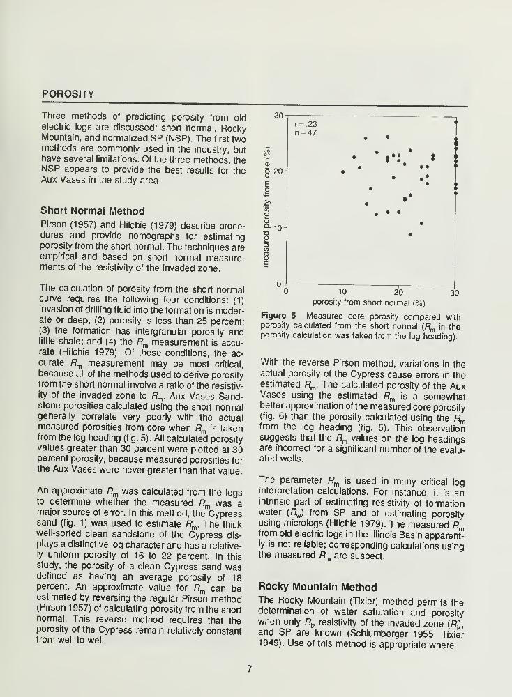
ity of the invaded zone to Rm . Aux Vases Sand-stone porosities calculated using the short normalgenerally correlate very poorly with the actualmeasured porosities from core when Rm is takenfrom the log heading (fig. 5). All calculated porosityvalues greater than 30 percent were plotted at 30percent porosity, because measured porosities forthe Aux Vases were never greater than that value.

An approximate Rm was calculated from the logsto determine whether the measured Rm was amajor source of error. In this method, thetypresssand (fig. 1) was used to estimate Rm . The thick

well-sorted clean sandstone of the Cypress dis-

plays a distinctive log character and has a relative-

ly uniform porosity of 16 to 22 percent. In this

study, the porosity of a clean Cypress sand wasdefined as having an average porosity of 18percent. An approximate value for Rm can beestimated by reversing the regular Pirson method(Pirson 1957) of calculating porosity from the shortnormal. This reverse method requires that theporosity of the Cypress remain relatively constantfrom well to well.

30r = .23

n = 47

<D

o20

Ep

go°- 10"DCDL.

COcoa>

E

• r: *t

• • ••

3010 20porosity from short normal (%)

Figure 5 Measured core porosity compared withporosity calculated from the short normal (Rm in theporosity calculation was taken from the log heading).

With the reverse Pirson method, variations in theactual porosity of the Cypress cause errors in theestimated Rm . The calculated porosity of the AuxVases using the estimated Rm is a somewhatbetter approximation of the measured core porosity(fig. 6) than the porosity calculated using the Rmfrom the log heading (fig. 5). This observationsuggests that the Rm values on the log headingsare incorrect for a significant number of the evalu-ated wells.

The parameter Rm is used in many critical log

interpretation calculations. For instance, it is anintrinsic part of estimating resistivity of formationwater (flj from SP and of estimating porosityusing micrologs (Hilchie 1979). The measured Rmfrom old electric logs in the Illinois Basin apparently is not reliable; corresponding calculations usingthe measured Rm are suspect.

Rocky Mountain MethodThe Rocky Mountain (Tixier) method permits thedetermination of water saturation and porositywhen only Rv resistivity of the invaded zone {R),and SP are known (Schlumberger 1955, Tixier

1949). Use of this method is appropriate where

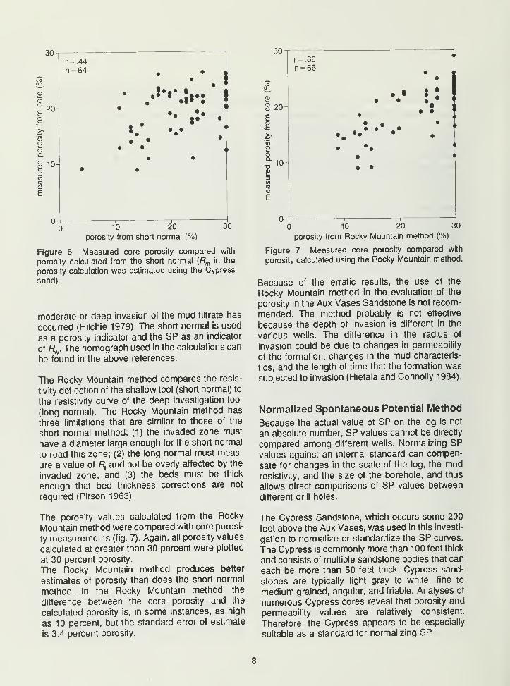
3U-r = .44

n == 64 • •

g•

CD

o•

.'••.If:g 20- •

•• *•o f. •>. I • _•

• •inO • •

o • •CL

• •

| 10-• •3

V)mCD

E

10 20

porosity from short normal (%)

30

Figure 6 Measured core porosity compared with

porosity calculated from the short normal (Rm in the

porosity calculation was estimated using the Cypress

sand).

moderate or deep invasion of the mud filtrate has

occurred (Hilchie 1979). The short normal is used

as a porosity indicator and the SP as an indicator

of f?w . The nomograph used in the calculations can

be found in the above references.

The Rocky Mountain method compares the resis-

tivity deflection of the shallow tool (short normal) to

the resistivity curve of the deep investigation tool

(long normal). The Rocky Mountain method has

three limitations that are similar to those of the

short normal method: (1) the invaded zone must

have a diameter large enough for the short normal

to read this zone; (2) the long normal must meas-

ure a value of fl; and not be overly affected by the

invaded zone; and (3) the beds must be thick

enough that bed thickness corrections are not

required (Pirson 1963).

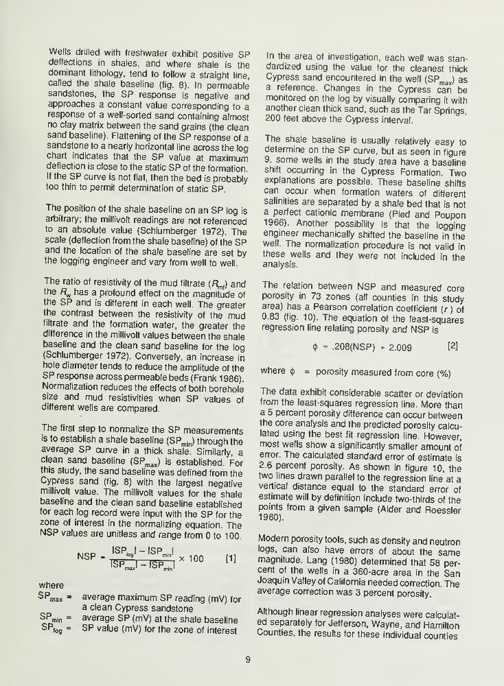
The porosity values calculated from the Rocky

Mountain method were compared with core porosi-

ty measurements (fig. 7). Again, all porosity values

calculated at greater than 30 percent were plotted

at 30 percent porosity.

The Rocky Mountain method produces better

estimates of porosity than does the short normal

method. In the Rocky Mountain method, the

difference between the core porosity and the

calculated porosity is, in some instances, as high

as 10 percent, but the standard error of estimate

is 3.4 percent porosity.

3Ur= .66

ii

n == 66•

•IICo" Io

CD •• ••

:• :

8 20-• ! i

E • Os

, : .• „•• n

>* •• •• ••

55o • •• ii

o • i

T3CD

• •i_3wcoCD

E

O- i i

10 20 30

porosity from Rocky Mountain method (%)

Figure 7 Measured core porosity compared with

porosity calculated using the Rocky Mountain method.

Because of the erratic results, the use of the

Rocky Mountain method in the evaluation of the

porosity in the Aux Vases Sandstone is not recom-

mended. The method probably is not effective

because the depth of invasion is different in the

various wells. The difference in the radius of

invasion could be due to changes in permeability

of the formation, changes in the mud characteris-

tics, and the length of time that the formation was

subjected to invasion (Hietala and Connolly 1984).

Normalized Spontaneous Potential Method

Because the actual value of SP on the log is not

an absolute number, SP values cannot be directly

compared among different wells. Normalizing SPvalues against an internal standard can compen-

sate for changes in the scale of the log, the mudresistivity, and the size of the borehole, and thus

allows direct comparisons of SP values between

different drill holes.

The Cypress Sandstone, which occurs some 200

feet above the Aux Vases, was used in this investi-

gation to normalize or standardize the SP curves.

The Cypress is commonly more than 1 00 feet thick

and consists of multiple sandstone bodies that can

each be more than 50 feet thick. Cypress sand-

stones are typically light gray to white, fine to

medium grained, angular, and friable. Analyses of

numerous Cypress cores reveal that porosity and

permeability values are relatively consistent.

Therefore, the Cypress appears to be especially

suitable as a standard for normalizing SP.

8

Wells drilled with freshwater exhibit positive SPdeflections in shales, and where shale is thedominant lithology, tend to follow a straight line,

called the shale baseline (fig. 8). In permeablesandstones, the SP response is negative andapproaches a constant value corresponding to aresponse of a well-sorted sand containing almostno clay matrix between the sand grains (the cleansand baseline). Flattening of the SP response of asandstone to a nearly horizontal line across the logchart indicates that the SP value at maximumdeflection is close to the static SP of the formation.If the SP curve is not flat, then the bed is probablytoo thin to permit determination of static SP.

The position of the shale baseline on an SP log is

arbitrary; the millivolt readings are not referencedto an absolute value (Schlumberger 1972). Thescale (deflection from the shale baseline) of the SPand the location of the shale baseline are set bythe logging engineer and vary from well to well.

The ratio of resistivity of the mud filtrate (/?ml) andthe Rw has a profound effect on the magnitude ofthe SP and is different in each well. The greaterthe contrast between the resistivity of the mudfiltrate and the formation water, the greater thedifference in the millivolt values between the shalebaseline and the clean sand baseline for the log(Schlumberger 1972). Conversely, an increase inhole diameter tends to reduce the amplitude of theSP response across permeable beds (Frank 1986).Normalization reduces the effects of both boreholesize and mud resistivities when SP values ofdifferent wells are compared.

The first step to normalize the SP measurementsis to establish a shale baseline (SPmin ) through theaverage SP curve in a thick shale. Similarly aclean sand baseline (SPmax ) is established. Forthis study, the sand baseline was defined from theCypress sand (fig. 8) with the largest negativemillivolt value. The millivolt values for the shalebaseline and the clean sand baseline establishedfor each log record were input with the SP for thezone of interest in the normalizing equation. TheNSP values are unitless and range from to 100.

whereSP„max

SPmin

=

SPlog

=

average maximum SP reading (mV) fora clean Cypress sandstoneaverage SP (mV) at the shale baselineSP value (mV) for the zone of interest

In the area of investigation, each well was stan-dardized using the value for the cleanest thickCypress sand encountered in the well (SPmax) asa reference. Changes in the Cypress can bemonitored on the log by visually comparing it withanother clean thick sand, such as the Tar Springs,200 feet above the Cypress interval.

The shale baseline is usually relatively easy todetermine on the SP curve, but as seen in figure9, some wells in the study area have a baselineshift occurring in the Cypress Formation. Twoexplanations are possible. These baseline shiftscan occur when formation waters of differentsalinities are separated by a shale bed that is nota perfect cationic membrane (Pied and Poupon1966). Another possibility is that the loggingengineer mechanically shifted the baseline in thewell. The normalization procedure is not valid inthese wells and they were not included in theanalysis.

The relation between NSP and measured coreporosity in 73 zones (all counties in this studyarea) has a Pearson correlation coefficient (r ) of0.83 (fig. 10). The equation of the least-squaresregression line relating porosity and NSP is

4> - .208(NSP) + 2.009 [2]

where $ = porosity measured from core (%)

The data exhibit considerable scatter or deviationfrom the least-squares regression line. More thana 5 percent porosity difference can occur betweenthe core analysis and the predicted porosity calcu-lated using the best fit regression line. However,most wells show a significantly smaller amount oferror. The calculated standard error of estimate is

2.6 percent porosity. As shown in figure 10, thetwo lines drawn parallel to the regression line' at avertical distance equal to the standard error ofestimate will by definition include two-thirds of thepoints from a given sample (Alder and Roessler1960).

Modern porosity tools, such as density and neutronlogs, can also have errors of about the samemagnitude. Lang (1980) determined that 58 per-cent of the wells in a 360-acre area in the SanJoaquin Valley of California needed correction. Theaverage correction was 3 percent porosity.

Although linear regression analyses were calculat-ed separately for Jefferson, Wayne, and HamiltonCounties, the results for these individual counties

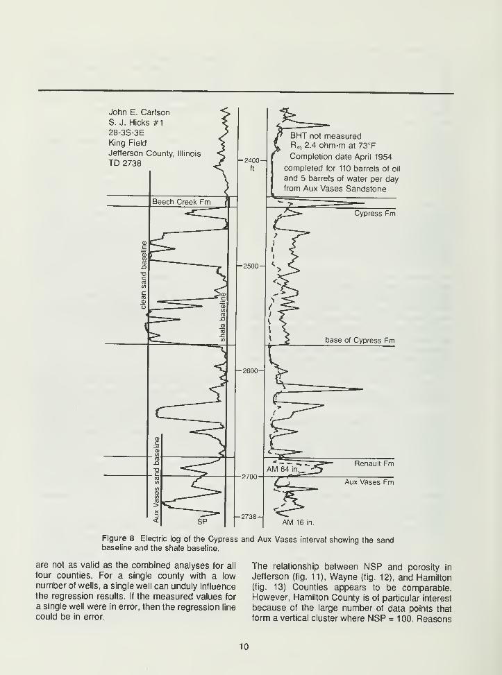
John E. Carlson

S. J. Hicks #128-3S-3E

King Field

Jefferson County, Illinois

TD 2738

BHT not measuredRm 2.4 ohm-m at 73°F

Completion date April 1954

completed for 110 barrels of oil

and 5 barrels of water per dayfrom Aux Vases Sandstone

AM 16 in.

Figure 8 Electric log of the Cypress and Aux Vases interval showing the sandbaseline and the shale baseline.

are not as valid as the combined analyses for all

four counties. For a single county with a lownumber of wells, a single well can unduly influence

the regression results. If the measured values for

a single well were in error, then the regression line

could be in error.

The relationship between NSP and porosity in

Jefferson (fig. 11), Wayne (fig. 12), and Hamilton(fig. 13) Counties appears to be comparable.However, Hamilton County is of particular interest

because of the large number of data points that

form a vertical cluster where NSP = 100. Reasons

10

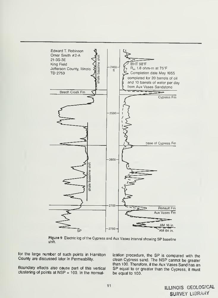
Edward T. Robinson

Omar Smith #2-A21-3S-3E

King Field

Jefferson County, Illinois

TD 2750

BHT 98°FRm 1.8 ohm-m at 75°F

Completion date May 1955

completed for 20 barrels of oil

and 10 barrels of water per dayfrom Aux Vases Sandstone

AM 64 in.

Figure 9 Electric log of the Cypress and Aux Vases interval showing SP baselineshift.

for the large number of such points in HamiltonCounty are discussed later in Permeability.

Boundary effects also cause part of this vertical

clustering of points at NSP = 100. In the normal-

ization procedure, the SP is compared with theclean Cypress sand. The NSP cannot be greaterthan 100. Therefore, if the Aux Vases Sand has anSP equal to or greater than the Cypress, it mustbe equal to 100.

11ILLINOIS GEOLOGICAL

SURVEY LIBRARY

standard error of estimatebest fit linear regression line

40 50 60 70

normalized SP8cT 90 100

Figure 10 Measured core porosity relative to NSP foralI

countiesiin study area. Two-thirds of data values wil

fall wrthin the bounds of the standard error of estimate

30

ooE 20o

ooQ.

o0)

r=.87n = 18

3CO03

E

10-

40 50 60 70 80normalized SP

90

Figure 11 Measured core porosity relative to NSP forJefferson County.

The best fit line, equation 2, should be used withsome caution when porosity is estimated. If coredata from the field indicate an average porosityhat is lower or higher than the predicted porosity

l?hct f inear/e9ression, core data should be

substituted on the plot and the curve modified Thedetermination of the Aux Vases porosity from thebP log in this study is based on a local empirical

30

v>ok.

oQ.

-a

2?

05

a>

E

20-

r = .74

n = 23

10

• •

40 50 60 70 80normalized SP

-I100

Figure 12 Measured core porosity relativeWayne County.

90

to NSP for

30

8 20Eo

r = .78

n = 28

• •

oQ.

o

c/>

CD(1)

E

10-

40

~1 1 r— 1-50 60 70 80

normalized SP90 100

HamTon3

CoMumy

SUredW POrOSi,y relatlVe t0 NSP ^

Somh"^-Th

feq

.

Uation definin9 this relationshipshould be used only for the four-county area forwhich it was derived. The technique should not beused with another formation or lithology without

Z« IT"t?10" °f the SP resP°nse to measuredcore data. The analysis was done on Aux Vasessandstones, and the results are not valid forlimestones.

12

PERMEABILITY

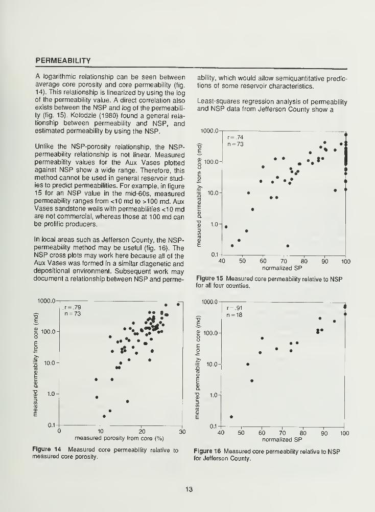
A logarithmic relationship can be seen betweenaverage core porosity and core permeability (fig.

14). This relationship is linearized by using the log

of the permeability value. A direct correlation also

exists between the NSP and log of the permeabili-

ty (fig. 15). Kolodzie (1980) found a general rela-

tionship between permeability and NSP, andestimated permeability by using the NSP.

Unlike the NSP-porosity relationship, the NSP-permeability relationship is not linear. Measuredpermeability values for the Aux Vases plotted

against NSP show a wide range. Therefore, this

method cannot be used in general reservoir stud-

ies to predict permeabilities. For example, in figure

15 for an NSP value in the mid-60s, measuredpermeability ranges from <10 md to >100 md. AuxVases sandstone wells with permeabilities <10 mdare not commercial, whereas those at 100 md canbe prolific producers.

In local areas such as Jefferson County, the NSP-permeability method may be useful (fig. 16). TheNSP cross plots may work here because all of theAux Vases was formed in a similar diagenetic anddepositional environment. Subsequent work maydocument a relationship between NSP and perme-

ability, which would allow semiquantitative predic-

tions of some reservoir characteristics.

Least-squares regression analysis of permeabilityand NSP data from Jefferson County show a

IUUU.U

r= .74 t

E,

n = 73 •

•1§ 100.0-

• •• •.«•

II

oE

•

•

II

ii

II

permeability

ob •

•

• •

• "

measured

b i•

••

•

•

0.1-i i i

i

40 50 60 70 80normalized SP

90 100

Figure 15 Measured core permeability relative to NSPfor all four counties.

1000.0

10 20measured porosity from core (%)

Figure 14 Measured core permeability relative to

measured core porosity.

30

1000.0

oE

2 100.0ooEo

= 10.0-Q03CD

ECDQ.

T3CD

C/5

coCD

E

LO-

OM-

r = .91

n = 18

11 1 1—

40 50 60 70 80normalized SP

90 100

Figure 16 Measured core permeability relative to NSPfor Jefferson County.

13

1000.0 1000.0-

40 50 60 70 80normalized SP

90 100 40 50

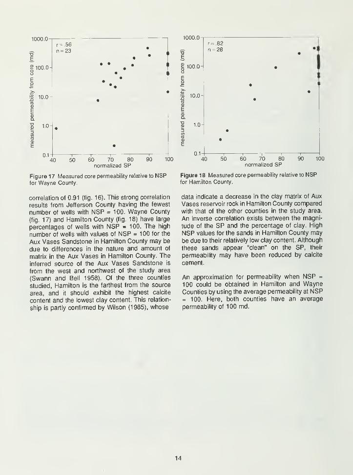
Figure 17 Measured core permeability relative to NSPfor Wayne County.

correlation of 0.91 (fig. 16). This strong correlation

results from Jefferson County having the fewest

number of wells with NSP = 100. Wayne County

(fig. 17) and Hamilton County (fig. 18) have large

percentages of wells with NSP = 100. The high

number of wells with values of NSP = 100 for the

Aux Vases Sandstone in Hamilton County may be

due to differences in the nature and amount of

matrix in the Aux Vases in Hamilton County. The

inferred source of the Aux Vases Sandstone is

from the west and northwest of the study area

(Swann and Bell 1958). Of the three counties

studied, Hamilton is the farthest from the source

area, and it should exhibit the highest calcite

content and the lowest clay content. This relation-

ship is partly confirmed by Wilson (1985), whose

60 70~~ 80normalized SP

100

Figure 18 Measured core permeability relative to

for Hamilton County.

NSP

data indicate a decrease in the clay matrix of Aux

Vases reservoir rock in Hamilton County compared

with that of the other counties in the study area.

An inverse correlation exists between the magni-

tude of the SP and the percentage of clay. High

NSP values for the sands in Hamilton County maybe due to their relatively low clay content. Although

these sands appear "clean" on the SP, their

permeability may have been reduced by calcite

cement.

An approximation for permeability when NSP =

100 could be obtained in Hamilton and WayneCounties by using the average permeability at NSP= 100. Here, both counties have an average

permeability of 100 md.

14

WATER SATURATION

Calculating accurate values of water saturation

(Sw ) for Aux Vases Sandstone from the dataavailable in Illinois has been a problem for years.

Water saturation values, including those calculatedfrom modern log suites, can be as high as 60 to

80 percent for wells in the Aux Vases Sandstonethat produce little or no water (Seyler 1988). Onthe other hand, some Aux Vases wells have highwater saturations and produce water. This greatvariability of Sw values in producing wells compli-cates the well evaluation process.

The high Sw values in producing wells are proba-bly caused by two factors: (1) the cementationexponent used in the formation factor relationship

of the Archie equation was too high (Archie 1942),and (2) clay was present in the formation.

The most common method used to calculate watersaturation in rocks that contain little clay in thematrix is the basic Archie equation (Archie 1942):

\ ft

[3]

where

Sw =

ftw =

ftt

=

F =

water saturation (%)resistivity of formation water (ohm-m)resistivity of the formation (ohm-m)formation factor

In the Archie equation 3,

F-_L(J)

m [4]

wherem = cementation exponent

<b = porosity (%)

The cementation exponent (m) is the most difficult

of the variables in the Archie equation to deter-mine. The value of m is dependent on pore geom-etry and equals 2 in sandstones that contain noclay matrix. In sandstones with a substantial

amount of clay, m can be as low as 1.7 (D. Hart-

mann, personal communication 1990). A commonmethod of compensating for the effects of clay onold electric logs was to vary the cementation

exponent. In some cases, a value of m as low as1.5 was used (Hilchie 1979). These low m valuesare not actual values measured from the rock;

however, low cementation exponent values canproduce realistic water saturations in shaly forma-tions. This method of using artificially low m valuesis basically a simplified version of the modernshaly sand calculations. The Aux Vases at KingField, which will be discussed latter, has clay in its

rock matrix. For this reason, the cementationexponent of the Aux Vases at King Field wasassigned a value of 1 .7.

Winsauer et al. (1952) showed that the cementa-tion exponent has lower values for better sorted,

slightly cemented sands than for those that areheavily cemented. Doveton (1986) also found thecementation exponent to be sensitive to the depo-sitional fabric or bedding of the rock. On a regional

scale, the Aux Vases will have significant varia-

tions in both the clay content and distribution of theclay in the pore throat, which will cause corre-sponding variations in m.

Pessimistic Sw values result from using m = 2 for

clean sandstone in the Archie equation when an m= 1 .7 better reflects the clay percentage. Constantm values should not be used on a regional basisfor calculating Sw from the Archie method or anyanalytical method that uses the cementationexponent. On a local scale, m should not varysignificantly, and reasonable water saturationvalues can be calculated using a constant valuefor m.

If the value of m is assumed to remain relatively

constant over an area, yet its value is unknown, aPickett plot or log-log plot of resistivity relative to

porosity values can be effectively used to estimatewater saturation (Pickett 1973, Lang 1973). ThePickett plot is a graphic derivation of the Archieequation. The initial step in analyzing well logsusing the Pickett plot method is to define the 100percent Sw zones on a log and use these zones in

defining resistivity of a formation 100 percentsaturated with formation water (ftj. The R valueswhen plotted relative to porosity establish the ft

line. All other water saturation percentages arecalculated from the initial R line. The slope of theft line on the Pickett plot reflects the value of m.

15

Note that the Pickett plot will work only if m stays

constant throughout the study area and the resis-

tivity tool has the same depth of investigation. Thelong normal (AM64) was used in this study. Meas-urements made with different types of tools cannotbe mixed together on a Pickett plot. For example,values of resistivity from the induction tool cannotbe used together with values from a long normaltool.

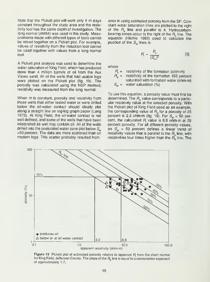
A Pickett plot analysis was used to determine the

water saturation of King Field, which has producedmore than 4 million barrels of oil from the AuxVases sand. All of the wells that had usable logs

were plotted on the Pickett plot (fig. 19). Theporosity was calculated using the NSP method;resistivity was measured from the long normal.

When m is constant, porosity and resistivity fromthose wells that either tested water or were drilled

below the oil-water contact should ideally plot

along a straight line on log-log graph paper (Lang

1973). At King Field, the oil-water contact is not

well defined, and some of the wells that have beeninterpreted as wet may contain oil. All of the wells

drilled into the postulated water zone plot below Sw>50 percent. The data are more scattered than onmodern logs. This scatter probably resulted from

error in using estimated porosity from the SP. Con-stant water saturation lines are plotted to the right

of the R line and parallel to it. Hydrocarbon-bearing zones occur to the right of the R line. Theequation (Hilchie 1982) used to calculate the

position of the Sw lines is

/*-R

(SJ<[5]

where

Sw =

resistivity of the formation (ohm-m)resistivity of the formation 100 percent

saturated with formation water (ohm-m)water saturation (%)

To use this equation, a porosity value must first bedetermined. The RQ value corresponds to a partic-

ular resistivity value at the selected porosity. Withthe Pickett plot of King Field used as an example,the corresponding value of f? for a porosity of 25percent is 2.2 ohm-m (fig. 19). For Sw = 50 per-

cent, the calculated /?, value is 8.8 ohm-m at 25percent porosity. For all different porosity values,

an Sw = 50 percent defines a linear trend of

resistivity values that is parallel to the R line, with

resistivities four times higher than the R line. The

100

55 10ooQ.

25% ^\ \ ^\

• produces oil

A below or at oil water contact

i

2.2 8.8i

0.1 1.0 10.0

apparent resistivity (ohm-m)100.0

Figure 19 Pickett plot of estimated porosity relative to apparent Rtfrom the short normal

for King Field, Jefferson County. The slope of the RQ line is equal to a cementation exponentof approximately 1.7.

16

same principle is used to establish any other Swpercentage.

The long normal can be used for the Pickett plot

analysis, since an actual ft, value is not necessaryand the long normal response commonly wasobtained from deep enough in the formation to

approximate fl,. If different wells are to be com-pared, then the resistivity tools must have a similar

electrode spacing and measure approximately thesame distance into the formation so that thePickett plot method will be valid. That the longnormal response may be from part of the invadedzone is ignored in the Pickett plot. Therefore, the

actual long normal values can usually be plotted

without having to take the invasion profile into

account.

In theory, the intercept of the RQ line at 100 per-

cent porosity should be the value of f?w . If theresistivity log is not measuring a true* ft,, theintercept will not be flw but instead will be a valuebetween R„ and Rmi . For King Field, the longnormal tool is not an accurate R

{measuring device

but is actually measuring part of the invaded zone.Because multiple wells have diverse R

mi values,the resistivity intercept at 100 percent porosity is

not a true Rw value.

17

SUMMARY

In Hamilton, Wayne, Franklin, and JeffersonCounties, the NSP technique was significantly

better than were the short normal and RockyMountain methods in predicting porosity in the AuxVases Sandstone. The NSP in relation to coreporosity had a correlation coefficient of 0.83. Theshort normal Rm from the log heading, short

normal Rm calculated, and Rocky Mountain meth-ods had correlation coefficients of 0.23, 0.44, and0.66, respectively. The measured Rm reported onold electric logs in the Illinois Basin is not a reliable

value, so calculations using Rm may be in error.

The NSP cannot be used to accurately predict

permeability. Although calculated values commonlyare the correct order of magnitude, but they usual-ly are not accurate enough for detailed reservoiranalysis.

Water saturations can be estimated by usingPickett plot analysis. The major advantage of

Pickett plots over the basic Archie equation is that

Pickett plots do not need the cementation expo-nent or the resistivity of the formation water to bepredefined.

18

REFERENCES

Alder, H. L, and E. B. Roessler, 1960, Introduction

to Probability and Statistics: W. H. Freeman &Company, San Francisco, California, 252 p.

Archie, G. E., 1942, The electrical resistivity log asan aid in determining some reservoir charac-

teristics: Transactions of the American Insti-

tute of Mechanical Engineers, v. 146, p.

54-62.

Bell, A. H., M. G. Oros, J. Van Den Berg, C. W.Sherman, and R. F. Mast, 1961, Petroleumindustry in Illinois, 1 960: Illinois State Geologi-

cal Survey, Illinois Petroleum 75, 121 p.

Buschbach, T. C, and D. R. Kolata, in press,

Regional setting of Illinois Basin, in M. W.Leighton, D. R. Kolata, D. F. Oltz, and J. J.

Eidel, editors, Interior Cratonic Basins (WorldPetroleum Basins series): The AmericanAssociation of Petroleum Geologists, Tulsa,

Oklahoma.Corelab, 1979, Fundamentals of Core Analysis:

Core Laboratories, Inc., 70 p.

Doveton, J. H., 1986, Log Analysis of SubsurfaceGeology Concepts and Computer Methods:John Wiley & Sons, New York, 273 p.

Frank, R. W., 1986, Prospecting with Old E-Logs:

Schlumberger Educational Services, Houston,Texas, 161 p.

Griffiths, J. C, 1952, Grain-size distribution andreservoir-rock characteristics: American Asso-ciation of Petroleum Geologists Bulletin, v. 36,

no. 2, p. 205-229.

Hietala, R. W., and E. T. Connolly, 1984, Well log

analysis methods and techniques in J. A.

Masters, editor, Elmworth, Case Study of aDeep Basin Gas Field: American Association

of Petroleum Geologists Memoir 38, p.

215-242.

Hilchie, D. W., 1979, Old Electric Log Interpreta-

tion: Institute for Energy Development, Tulsa,

Oklahoma, 161 p.

Hilchie, D. W., 1982, Advanced Well Log Interpre-

tation: Douglas W. Hilchie, Inc., Golden,Colorado, 208 p.

Howard, R. H., in press, Hydrocarbon reservoir

distribution, in M. W. Leighton, D. R. Kolata,

D. F. Oltz, and J. J. Eidel, editors, Interior

Cratonic Basins (World Petroleum Basinsseries): The American Association of Petro-

leum Geologists, Tulsa, Oklahoma.Kolodzie, S., 1980, Analysis of pore throat size

and use of the Waxman-Smits equation to

determine OOIP in Spindle Field, Colorado:presented at Society of Petroleum Engineers

meeting, Dallas, Texas, September 1980,SPE paper 9382.

Lang, W. H., 1973, Porosity-resistivity cross-plot-

ting: The Log Analyst, January-February, v.

14, no. 1., p. 16-20.

Lang, W. H., 1980, Porosity log calibrations: TheLog Analyst, March-April, v. 21, no. 2, p.

14-18.

McKay, R. H., 1980, A Depositional Model for the

Aux Vases Formation and the Joppa Memberof the Ste. Genevieve Formation (Mississippi-

an) in Southwestern Illinois and SoutheasternMissouri: M.S. thesis, Southern Illinois Univer-

sity, Carbondale, 184 p.

Pickett, G. R., 1973, Pattern recognition as ameans of formation evaluation: The LogAnalyst, July-August, v. 14, no. 4, p. 3-11.

Pied, B., and A. Poupon, 1966, SP base line shifts

in Algeria: Seventh Annual Society of Profes-

sional Well Log Analysts Symposium, Societyof Professional Well Log Analysts, Tulsa,

Oklahoma, p. 1H-12H.Pirson, S. J., 1957, Formation evaluation by log

interpretation: World Oil, April, May, June.Pirson, S. J., 1963, Handbook of Well Log Analy-

sis for Oil and Gas Formation Evaluation:

Prentice-Hall, Inc., Englewood Cliffs, NewJersey, 326 p.

Schlumberger, 1955, Log Interpretation Charts:

Schlumberger Limited, Houston, Texas, p.

D7-D8.Schlumberger, 1972, Schlumberger log interpreta-

tion, Volume 1—Principles: SchlumbergerLimited, Houston, Texas, 113 pp.

Seyler, B. J., 1988, Role of clay mineralogy in

water saturation; drilling, completion, andrecovery techniques, in C. W. Zuppann, B. D.

Keith, and S. J. Keller, editors, Geology andPetroleum Production of the Illinois Basin.

Volume 2: Indiana-Kentucky and Illinois Geo-logical Societies Joint Publication, p. 150.

Smoot, T. W., 1960, Clay mineralogy of pre-Penn-sylvanian sandstones and shales of the Illinois

Basin. Part III. Clay minerals of various facies

of some Chester formations: Illinois StateGeological Survey, Circular 293, 19 p.

Swann, D. H., and A. H. Bell, 1958, Habitat of oil

19

in the Illinois Basin, in L. G. Weeks, editor,

Habitat of Oil: The American Association of

Petroleum Geologists, Tulsa, Oklahoma, p.

447-472.

Tixier, M. P., 1949, Electric log analysis in the

Rocky Mountains: Oil and Gas Journal, June

23, p. 143-147, 217-219.

Weimer, R. J., J. D. Howard, and D. R. Lindsey,

1982, Tidal flats and associated tidal chan-

nels, in P. A. Scholle and D. Spearing, edi-

tors, Sandstone Depositional Environments:

American Association of Petroleum Geologists

Memoir 31, 410 p.

Wilson, B., 1985, Depositional Environments and

Diagenesis of Sandstone Facies in the AuxVases Formation (Mississippian), Illinois

Basin: M.S. thesis, Southern Illinois Universi-

ty, Carbondale, 130 p.

Winsauer, W. O., H. M. Shearin, Jr., P. H. Mas-

son, and M. Williams, 1952, Resistivity of

brine saturated sands in relation to pore

geometry: American Association of Petroleum

Geologists Bulletin, v. 36, no. 2, p. 253-277.

Young, V. R., 1983, Permeable Sand Body Trends

in the Aux Vases Formation, Buckner-Sesser-

Valier Fields, Franklin County, Illinois: M.S.

thesis, Southern Illinois University, Carbon-

dale, 79 p.

20

APPENDIX

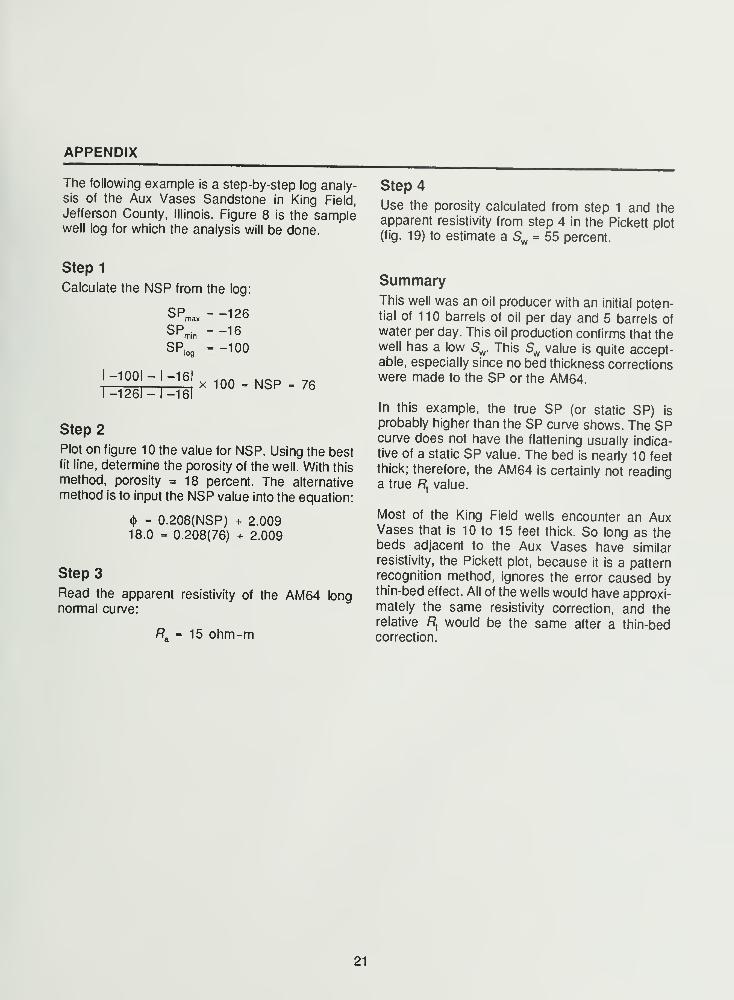
The following example is a step-by-step log analy-sis of the Aux Vases Sandstone in King Field,

Jefferson County, Illinois. Figure 8 is the samplewell log for which the analysis will be done.

Step 1

Calculate the NSP from the log:

SPma, - -126

SPn

SPlog

I -1001 -I -161

1-1261- 1-161

- -16

- -100

x 100 - NSP - 76

Step 2

Plot on figure 10 the value for NSP. Using the bestfit line, determine the porosity of the well. With this

method, porosity = 18 percent. The alternative

method is to input the NSP value into the equation:

<() = 0.208(NSP) + 2.00918.0 - 0.208(76) + 2.009

Step 3

Read the apparent resistivity of the AM64 longnormal curve:

ft, = 15 ohm-m

Step 4

Use the porosity calculated from step 1 and theapparent resistivity from step 4 in the Pickett plot

(fig. 19) to estimate a Sw = 55 percent.

SummaryThis well was an oil producer with an initial poten-tial of 1 1 barrels of oil per day and 5 barrels of

water per day. This oil production confirms that thewell has a low S„. This Sw value is quite accept-able, especially since no bed thickness correctionswere made to the SP or the AM64.

In this example, the true SP (or static SP) is

probably higher than the SP curve shows. The SPcurve does not have the flattening usually indica-

tive of a static SP value. The bed is nearly 10 feetthick; therefore, the AM64 is certainly not readinga true R

xvalue.

Most of the King Field wells encounter an AuxVases that is 10 to 15 feet thick. So long as thebeds adjacent to the Aux Vases have similar

resistivity, the Pickett plot, because it is a patternrecognition method, ignores the error caused bythin-bed effect. All of the wells would have approxi-mately the same resistivity correction, and therelative R

twould be the same after a thin-bed

correction.

21