Embed Size (px)
Citation preview

Application of Neural Networks to Inverter-Based Resources
Sidhaarth Venkatachari
Thesis submitted to the Faculty of theVirginia Polytechnic Institute and State University
in partial fulfillment of the requirements for the degree of
Master of Sciencein
Electrical Engineering
Ali Mehrizi-Sani, ChairJaime De La Reelopez
Chen-Ching Liu
April 30, 2021Blacksburg, Virginia
Keywords: Neural networks, support vector classifier, modular multilevel converters.Copyright 2021, Sidhaarth Venkatachari

Application of Neural Networks to Inverter-Based Resources
Sidhaarth Venkatachari
ABSTRACT
With the deployment of sensors in hardware equipment and advanced metering infrastruc-ture, system operators have access to unprecedented amounts of data. Simultaneously,grid-connected power electronics technology has had a large impact on the way electricalenergy is generated, transmitted, and delivered to consumers. Artificial intelligence andmachine learning can help address the new power grid challenges with enhanced computa-tional abilities and access to large amounts of data. This thesis discusses the fundamentalsof neural networks and their applications in power systems such as load forecasting, powersystem stability analysis, and fault diagnosis. It extends application of neural networksto inverter-based resources by studying the implementation and performance of a neuralnetwork controller emulator for voltage-sourced converters. It delves into how neural net-works could enhance cybersecurity of a component through multiple hardware and softwareimplementations of the same component. This ensures that vulnerabilities inherent in oneform of implementation do not affect the system as a whole. The thesis also proposes acomprehensive support vector classifier (SVC)–based submodule open-circuit fault detectionand localization method for modular multilevel converters. This method eliminates the needfor extra hardware. Its efficacy is discussed through simulation studies in PSCAD/EMTDCsoftware. To ensure efficient usage of neural networks in power system simulation softwares,this thesis entails the step by step implementation of a neural network custom componentin PSCAD/EMTDC. The custom component simplifies the process of recreating a neuralnetwork in PSCAD/EMTDC by eliminating the manual assembly of predefined library com-ponents such as summers, multipliers, comparators, and other miscellaneous blocks.
Application of Neural Networks to Inverter-Based Resources
Sidhaarth Venkatachari
GENERAL AUDIENCE ABSTRACT
Data analytics and machine learning play an important role in the power grids of today,which are continuously evolving with the integration of renewable energy resources. It isexpected that by 2030 most of the electric power generated will be processed by some formof power electronics, e.g., inverters, from the point of its generation. Machine learning hasbeen applied to various fields of power systems such as load forecasting, stability analysis, andfault diagnosis. This work extends machine learning applications to inverter-based resourcesby using artificial neural networks to perform controller emulation for an inverter, providecybersecurity through heterogeneity, and perform submodule fault detection in modularmultilevel converters. The thesis also discusses the step by step implementation of a neuralnetwork custom component in PSCAD/EMTDC software. This custom component simplifiesthe process of creating a neural network in PSCAD/EMTDC by eliminating the manualassembly of predefined library components.

Dedication
This work is dedicated to my amma (mother) Indu
iv

Acknowledgments
I did not expect to finish a major portion of my graduate life in a pandemic and I amdeeply grateful to all the people who have made this possible. First and foremost, I wouldlike to convey my profound gratitude to my research advisor and committee chair, Dr. AliMehrizi-Sani. Thank you for always finding the time to discuss my new ideas, clarifying myquestions, and gently guiding me whenever I got carried away and had selfdoubt. You havebeen one of my best teachers and I should mention here that I thoroughly enjoyed enrollingin your HVDC/FACTS course. I greatly value our discussions and your pertinent inputson things such as presentation would help me greatly as I transition to corporate life atDominion Energy.
I wish to thank Dr. Jaime De La Ree and Dr. Chen-Ching Liu for nurturing a welcomingatmosphere for the graduate students at PEC. To Dr. De La Ree, I relished working asyour GTA for two semesters and cherish our conversations on various topics. Thank youvery much for helping me in my search for internships during my first year in graduate school.
I am grateful for the friendships and interactions with other graduate students at the PEC– Alok, Imtiaj, Nick, Sangeetha, Vivek, Biqi, Tapas, Rounak, Sarthak, and Shuchismita. ToArdavan, I am immensely grateful for your guidance on technical matters and softwares. Ienjoyed working with you on the MMC project this semester. To Manish, thank you forbeing a phone call away and providing constructive feedback and support. To Rahul andFaris, cheers to the meet-ups throughout graduate school. It would be remiss not to thankmy close friends Abhijit, Naarayanan, and Navaneet for providing emotional support, creat-ing fond memories, and always being there for me.
Finally, I would like to thank my loving and supporting family – my parents Indu andVenkat, my grandparents Usha and Ravi, my brother Sanjhay and my aunt (chithi) Sudha.Thank you lending a patient ear and providing counsel to all my problems both academicand nonacademic. My sincerest gratitutde to all of you for always looking out for me andkeeping me in your prayers. I certainly can’t thank my amma (mother) Indu enough. Youare my role model and my inspiration. I will definitely not be where I am without yourendless sacrifices and the unconditional love that you showered on me. To you I dedicatethis thesis.
v
Contents
List of Figures ix
List of Tables xi
1 Introduction 1
1.1 Biological and Artificial Neuron . . . . . . . . . . . . . . . . . . . . . . . . . 2
1.2 Application of NNs . . . . . . . . . . . . . . . . . . . . . . . . . . . . . . . . 5
1.2.1 NN for Power Electronics . . . . . . . . . . . . . . . . . . . . . . . . 5
1.2.2 NN for Load Forecasting . . . . . . . . . . . . . . . . . . . . . . . . . 5
1.2.3 NN for Fault Diagnosis . . . . . . . . . . . . . . . . . . . . . . . . . . 6
1.2.4 NN for Stability Analysis . . . . . . . . . . . . . . . . . . . . . . . . 6
1.2.5 NN for Controller Emulation . . . . . . . . . . . . . . . . . . . . . . 7
1.2.6 NN for Power System Component(s) Modeling . . . . . . . . . . . . . 7
1.3 NN for Cybersecurity . . . . . . . . . . . . . . . . . . . . . . . . . . . . . . . 10
1.4 Thesis Outline . . . . . . . . . . . . . . . . . . . . . . . . . . . . . . . . . . 11
2 NN Custom Component in PSCAD 13
2.1 Parameters of the NN Custom Component . . . . . . . . . . . . . . . . . . . 13
2.2 Activation Function Choices . . . . . . . . . . . . . . . . . . . . . . . . . . . 16
2.3 NNCC Procedure . . . . . . . . . . . . . . . . . . . . . . . . . . . . . . . . . 19
2.3.1 Interfacing Challenges . . . . . . . . . . . . . . . . . . . . . . . . . . 20
2.4 Logic behind Code . . . . . . . . . . . . . . . . . . . . . . . . . . . . . . . . 20
2.4.1 Preconditioning of Weights and Biases . . . . . . . . . . . . . . . . . 20
2.4.2 Dimension Creation . . . . . . . . . . . . . . . . . . . . . . . . . . . 21
2.4.3 Recursive Referenced Calling . . . . . . . . . . . . . . . . . . . . . . 21
2.5 Preparation of Weights and Biases . . . . . . . . . . . . . . . . . . . . . . . 22
vi

3 NN Emulator for VSC Controller 24
3.1 Implementation of the NN Controller Emulator . . . . . . . . . . . . . . . . 24
3.1.1 Importance of Data Scaling . . . . . . . . . . . . . . . . . . . . . . . 25
3.1.2 Building the Model . . . . . . . . . . . . . . . . . . . . . . . . . . . . 25
3.1.3 Compiling the Model . . . . . . . . . . . . . . . . . . . . . . . . . . . 26
3.1.4 Training the Model . . . . . . . . . . . . . . . . . . . . . . . . . . . . 26
3.2 Performance Evaluation . . . . . . . . . . . . . . . . . . . . . . . . . . . . . 27
3.2.1 Step Change in Direct Axis Current Reference . . . . . . . . . . . . . 27
3.2.2 Step Change in Quadratic Axis Reference . . . . . . . . . . . . . . . 27
3.2.3 Single-Phase to Ground Fault at PCC . . . . . . . . . . . . . . . . . 27
3.2.4 Increasing SCR by a Factor of 10 . . . . . . . . . . . . . . . . . . . . 28
3.3 Conclusions . . . . . . . . . . . . . . . . . . . . . . . . . . . . . . . . . . . . 28
4 Cybersecurity in VSC 30
4.1 The Voltage-Sourced Converter . . . . . . . . . . . . . . . . . . . . . . . . . 31
4.2 AI and Cybersecurity . . . . . . . . . . . . . . . . . . . . . . . . . . . . . . . 32
4.3 Proposed Method . . . . . . . . . . . . . . . . . . . . . . . . . . . . . . . . . 33
4.4 Performance Evaluation . . . . . . . . . . . . . . . . . . . . . . . . . . . . . 35
4.5 Conclusions . . . . . . . . . . . . . . . . . . . . . . . . . . . . . . . . . . . . 36
5 Submodule Fault Detection in MMCs using Support Vector Classification 38
5.1 Introduction . . . . . . . . . . . . . . . . . . . . . . . . . . . . . . . . . . . . 38
5.2 SM Faults in MMCs . . . . . . . . . . . . . . . . . . . . . . . . . . . . . . . 40
5.2.1 Overview of MMC Modeling and Control . . . . . . . . . . . . . . . 40
5.2.2 Double-Switch Open Circuit Faults in MMCs . . . . . . . . . . . . . 42
5.3 Proposed SM Fault Detection Method . . . . . . . . . . . . . . . . . . . . . 44
5.3.1 SVC-Based Fault Detection Method . . . . . . . . . . . . . . . . . . 44
5.4 Performance Evaluation . . . . . . . . . . . . . . . . . . . . . . . . . . . . . 46
5.5 Conclusions . . . . . . . . . . . . . . . . . . . . . . . . . . . . . . . . . . . . 47
vii

6 Contributions and Future Work 50
Bibliography 51
viii

List of Figures
1.1 A basic NN with 4 inputs, 2 outputs, and 1 hidden layer. . . . . . . . . . . . 2
1.2 Structure and parts of a biological neuron [1]. . . . . . . . . . . . . . . . . . 3
1.3 Structure and components of an artificial neuron. . . . . . . . . . . . . . . . 4
1.4 NN controller emulator for a controller and plant feedback system. . . . . . . 7
1.5 Connection of renewables to the grid using power electronic devices [2]. . . . 8
1.6 Futuristic power grid with high renewable penetration and an NN used tocapture the behavior of a renewable energy device installed in a house. . . . 9
2.1 Parameters of the NNCC. . . . . . . . . . . . . . . . . . . . . . . . . . . . . 14
2.2 (a) NNCC with 4 inputs and 3 outputs, (b) NNCC with 10 inputs and 10outputs, (c) NNCC with array outputs, and (d) NNCC with individual outputs. 15
2.3 Enabling entering of neurons in the second hidden layer using conditionalstatements in the NNCC component defintion in PSCAD. . . . . . . . . . . 16
2.4 Activation functions - (a) Binary step, (b) Linear, (c) Sigmoid, (d) Tanh, (e)Relu, (f) Leaky relu, and (g) Swish. . . . . . . . . . . . . . . . . . . . . . . . 17
2.5 NNCC procedure describing the flow of parameters and inputs from PSCADto C and outputs from C to PSCAD. . . . . . . . . . . . . . . . . . . . . . . 19
2.6 Creation of the NN in C. . . . . . . . . . . . . . . . . . . . . . . . . . . . . . 21
2.7 Preparation of weights and biases (single space format). . . . . . . . . . . . . 22
2.8 Preparation of weights and biases (line format). . . . . . . . . . . . . . . . . 23
2.9 Preparation of weights and biases (tab format). . . . . . . . . . . . . . . . . 23
3.1 (a) id tracking by the NN emulator for step changes in id ref and (b) iq trackingby the NN emulator for step changes in id ref. . . . . . . . . . . . . . . . . . . 27
3.2 (a) iq tracking by the NN emulator for step changes in iq ref and (b) id trackingby the NN emulator for step changes in iq ref. . . . . . . . . . . . . . . . . . . 28
3.3 id tracking by the NN emulator for a single-phase AG fault at the PCC. . . . 28
3.4 id tracking by the NN emulator for a change in the SCR. . . . . . . . . . . . 29
ix
4.1 Block diagram demonstration of the VSC and its control. . . . . . . . . . . . 31
4.2 Proposed NN for cybersecurity. . . . . . . . . . . . . . . . . . . . . . . . . . 34
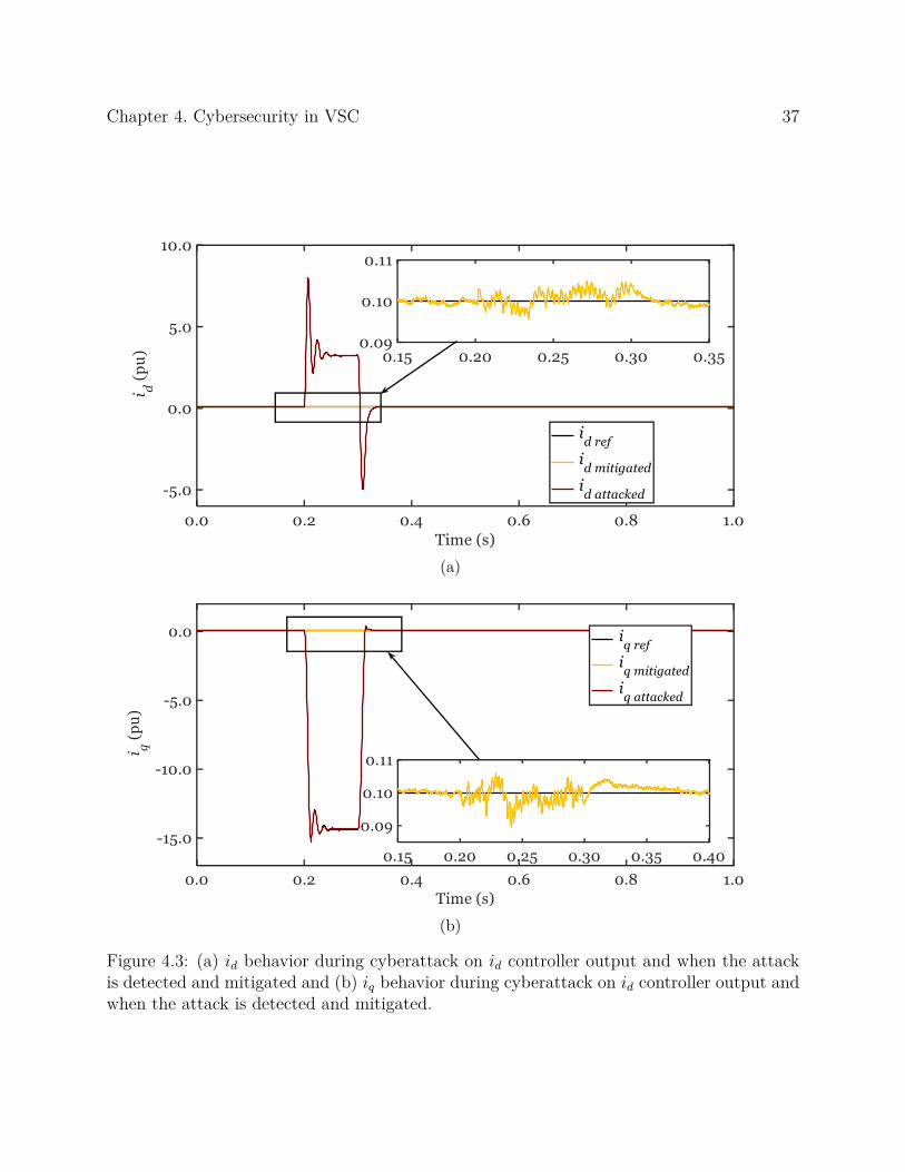
4.3 (a) id behavior during cyberattack on id controller output and when the at-tack is detected and mitigated and (b) iq behavior during cyberattack on idcontroller output and when the attack is detected and mitigated. . . . . . . 37
5.1 Three-phase MMC. . . . . . . . . . . . . . . . . . . . . . . . . . . . . . . . . 40
5.2 SHE-PWM MMC controller. . . . . . . . . . . . . . . . . . . . . . . . . . . . 42
5.3 Proposed SVC fault detection method. . . . . . . . . . . . . . . . . . . . . . 43
5.4 Number of times VCSM1is maximum in a time period. . . . . . . . . . . . . . 45
5.5 Classification of sample support vectors using a hyper-plane. . . . . . . . . . 45
5.6 (a) MMC capacitor voltages during double-switch OC faults, (b) MMC armcurrents during double-switch OC faults, and . . . . . . . . . . . . . . . . . 48
5.6 (c) Bypass signal produced by the SVC. . . . . . . . . . . . . . . . . . . . . 49
x

List of Tables
1.1 Comparison between the parts of a biological and an artificial neuron. . . . . 4
3.1 Behavior of mean absolute error (MAE) and loss function as the NN emulatorcycles through the training data. . . . . . . . . . . . . . . . . . . . . . . . . 26
4.1 Parameters of VSC for simulation. . . . . . . . . . . . . . . . . . . . . . . . 35
4.2 Parameters of the VSC controller for simulation. . . . . . . . . . . . . . . . . 35
5.1 SM behavior under double-switch OC faults . . . . . . . . . . . . . . . . . . 43
5.2 Parameters of the MMC for simulation. . . . . . . . . . . . . . . . . . . . . . 46
xi
Chapter 1
Introduction
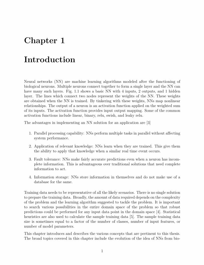
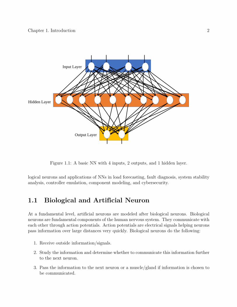
Neural networks (NN) are machine learning algorithms modeled after the functioning ofbiological neurons. Multiple neurons connect together to form a single layer and the NN canhave many such layers. Fig. 1.1 shows a basic NN with 4 inputs, 2 outputs, and 1 hiddenlayer. The lines which connect two nodes represent the weights of the NN. These weightsare obtained when the NN is trained. By tinkering with these weights, NNs map nonlinearrelationships. The output of a neuron is an activation function applied on the weighted sumof its inputs. The activation function provides input output mapping. Some of the commonactivation functions include linear, binary, relu, swish, and leaky relu.
The advantages in implementing an NN solution for an application are [3]
1. Parallel processing capability: NNs perform multiple tasks in parallel without affectingsystem performance.
2. Application of relevant knowledge: NNs learn when they are trained. This give themthe ability to apply that knowledge when a similar real time event occurs.
3. Fault tolerance: NNs make fairly accurate predictions even when a neuron has incom-plete information. This is advantageous over traditional solutions that need completeinformation to act.
4. Information storage: NNs store information in themselves and do not make use of adatabase for the same.
Training data needs to be representative of all the likely scenarios. There is no single solutionto prepare the training data. Broadly, the amount of data required depends on the complexityof the problem and the learning algorithm suggested to tackle the problem. It is importantto search various possibilities in the entire domain space of the problem so that robustpredictions could be performed for any input data point in the domain space [4]. Statisticalheuristics are also used to calculate the sample training data [5]. The sample training datasize is sometimes equal to a factor of the number of classes, number of input features, ornumber of model parameters.
This chapter introduces and describes the various concepts that are pertinent to this thesis.The broad topics covered in this chapter include the evolution of the idea of NNs from bio-
1
Chapter 1. Introduction 2
Input Layer
Hidden Layer
Output Layer
Figure 1.1: A basic NN with 4 inputs, 2 outputs, and 1 hidden layer.
logical neurons and applications of NNs in load forecasting, fault diagnosis, system stabilityanalysis, controller emulation, component modeling, and cybersecurity.
1.1 Biological and Artificial Neuron
At a fundamental level, artificial neurons are modeled after biological neurons. Biologicalneurons are fundamental components of the human nervous system. They communicate witheach other through action potentials. Action potentials are electrical signals helping neuronspass information over large distances very quickly. Biological neurons do the following:
1. Receive outside information/signals.
2. Study the information and determine whether to communicate this information furtherto the next neuron.
3. Pass the information to the next neuron or a muscle/gland if information is chosen tobe communicated.

Chapter 1. Introduction 3
Figure 1.2: Structure and parts of a biological neuron [1].
Fig. 1.2 shows the pictorial representation of a biological neuron with its various parts. Aneuron comprises of three main parts along with an external synapse. Their functions areas follows:
1. Dendrites: These obtain signals from the previous neuron for processing.
2. Neuron cell body: These process the input signals obtained by the dendrites and makea decision on whether the signal should be passed further to the next neuron/musclegland.
3. Axon: These transmit the processed signal from the neuron cell body to the tip of theneuron.
4. Synapse: These provide the connection between the axon of one neuron and the den-drite of the next.
The incoming signals to a particular neuron can trigger them to fire (an excitatory signal) orinhibit them from firing (an inhibitory signal). A single neuron receives thousands of suchelectrical impulse inputs through its dendrites and decides to fire depending on the sum ofthe inhibitory and excitatory signals that it receives. This process happens inside the cellbody of the neuron. If the neuron decides to fire, the signal is transmitted down its axon.
Chapter 1. Introduction 4
Input Layer
Input Weights
w1
w2
w3
w4
Activation function
Σf()
Output
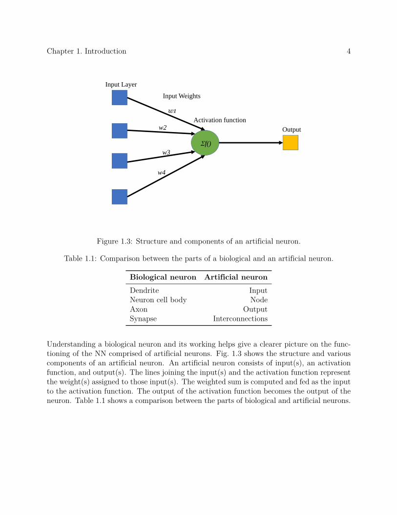
Figure 1.3: Structure and components of an artificial neuron.
Table 1.1: Comparison between the parts of a biological and an artificial neuron.
Biological neuron Artificial neuronDendrite InputNeuron cell body NodeAxon OutputSynapse Interconnections
Understanding a biological neuron and its working helps give a clearer picture on the func-tioning of the NN comprised of artificial neurons. Fig. 1.3 shows the structure and variouscomponents of an artificial neuron. An artificial neuron consists of input(s), an activationfunction, and output(s). The lines joining the input(s) and the activation function representthe weight(s) assigned to those input(s). The weighted sum is computed and fed as the inputto the activation function. The output of the activation function becomes the output of theneuron. Table 1.1 shows a comparison between the parts of biological and artificial neurons.

Chapter 1. Introduction 5
1.2 Application of NNs
1.2.1 NN for Power Electronics
NNs have been used for control and estimation applications in power electronics. Spacevector PWM (SVM) technique is used for a three-phase machine with two-level voltage-fedinverter. Generally, this SVM algorithm is implemented through digital signal processors.Reference [6] presents a neural network implementation of SVM to fasten its implementationthereby helping increase converter switching frequency. This is useful particularly when anapplication-specific integrated circuit chip is used in the modulator. Reference [7] presents ahybrid of the recurrent neural network and a feedforward neural network for flux estimationof induction motor drives. This ensures superior transient performance to the standard DSP-based programmable cascaded low pass filter traditionally used to perform flux estimation.Reference [8] presents a feedforward neural network to estimate feedback signals in inductionmotor drive systems. It receives the machine terminal signals and computes flux and torqueat the output which is used to control the motor drive system.
1.2.2 NN for Load Forecasting
NNs are useful to forecast loads because of their ability to figure out complex relationshipsbetween multiple inputs and outputs. Reference [9] presents an NN load forecasting modelto predict daily load profiles for 7 days of the week including holidays. BackpropagationNN is used for the above application. Reference [10] presents a short term load forecastingmodel using NN for the University of Petronas (UTP). A multilayer perceptron (MLP)is used to predict week ahead electricity loads. Due to large changes in the electricityconsumption, regression methods perform poorly. The MLP is able to overcome this problemdue to its architecture. Reference [11] presents an NN load forecasting model that uses theridge activation function. These are constructed using Meyer wavelets. Genetic algorithmtechniques are used for training. Reference [12] uses correlation analysis to determine whichparameters are inputted to the forecasting model. This is helpful in reducing redundancies.Reference [13] filters weakly correlated attributes using condition analysis and trains theNN using momentum method to prevent convergence to the local minimum. Reference [14]uses principal component analysis to perform correlation and uses normalization to avoidNN saturation. Reference [15] compares the radial basis function NN (RBFNN) with theMLP for load forecasting applications. The RBFNN requires fewer weights and biases torepresent the mapping whereas the MLP has a lower error when the number of hidden layersis between 5 and 10.

Chapter 1. Introduction 6
1.2.3 NN for Fault Diagnosis
NNs are useful to locate and classify faults. Reference [16] uses a fuzzy wavelet NN (FWNN)for fault diagnosis of power transformers. It combines the benefits of robust classificationby the FWNN with weighted least squares and uses knowledge reduction to simplify theinput points as well as the number of parameters fed to the FWNN. Reference [17] uses thediscrete wavelet transform (DWT) with backpropogation NN to diagnose and classify faultsby considering the energy distributions characteristic to different kinds of faults. The weightsare modified based on the difference between the predicted outputs and the actual outputson the training data. The downside is that backpropagation NNs require a lot of time totrain. Reference [18] uses NN classification to find out the type of power system transientscaused by short circuit, switching of breakers, and lightning disturbances. Wavelet transformis used to extract the features that are fed into the backpropagation NN (BPNN). Reference[19] uses a distribution state estimation technique with gaussian mixture models to generatepseudo measurements from load flow simulations. The variance between the predicted andthe actual measurements is used to diagnose faults.
1.2.4 NN for Stability Analysis
NNs have widespread application in power system stability analysis. Reference [19] usesa single NN to establish the relationship between power system operating conditions andvoltage stability margin by computing the ‘mathematical distance’ between the two. It usesorthogonalization to find out which inputs have a higher impact on accuracy. Reference[20] uses an MLP with 5 hidden neurons to perform power system voltage stability analysis.Random feasible data inputs are fed and for each data point, the P margin is generatedwhich serves as the voltage stability index. This approach predicts stability both duringa normal scenario as well as an N − 1 contingency scenario. Reference [21] uses an NNcontroller for the unified power flow controller (UPFC) to enhance its transient stability. Ituses backpropagation with the Levenberg–Marquardt (LM) method to enhance convergence.Reference [21] showed that NNs could model systems with high nonlinearity. The approachuses the quadrature component of the series voltage injected and the active power of the twoprior time steps. The ANN built is a feedforward NN with one hidden layer comprising of15 neurons (sigmoid activation), 4 inputs, and 1 output. Reference [22] uses a probabilisticNN (PNN) to distinguish the inrush magnetizing phenomenon from the fault of a powertransformer from a transient analysis point of view. To determine which of the above phe-nomenon is occurring, it uses two parameters - voltage to frequency ratio and the maximumvalue of differential current. This PNN does not require validation data but requires thatthe user determine a smoothing parameter. Reference [23] uses the S transform to extractfeatures that would determine power quality. The features extracted are applied to an ANNto classify the kind of PQ disturbance. This approach is effective in identifying the kind ofPQ disturbance.

Chapter 1. Introduction 7
1.2.5 NN for Controller Emulation
PlantReference
Controller
Neural
Network
Controller
X(k) Y(k)
Output
e(k)
error
+-
+-
Figure 1.4: NN controller emulator for a controller and plant feedback system.
Fig. 1.4 shows how an NN controller could replace an actual controller in a plant and con-troller feedback system. The controller can be complicated or simple, static or dynamic. TheNN controller is trained to emulate the actual controller. The NN weights are optimizedby reducing the error between the actual controller output and the NN controller emulatoroutput. The NN controller could then replace the actual controller and the dynamic perfor-mance of the NN controller emulator and plant system could be studied. The plant couldbe any power system component/power electronic device such as a VSC. The NN controllercan be retrained online for plant parameter variation to make it adaptive. Normally utilizedcontrollers such as PI, PID, and PD are static and nonlinear. These controllers can be re-placed by the NN controller since they are dependent on a nonlinear mapping of inputs andoutputs.
1.2.6 NN for Power System Component(s) Modeling
NNs form an important part of any predictive analysis. The current power grid analysis islargely model driven. A data driven NN approach can supplement the model driven approachwhile providing additional benefits. Reference [24] uses NNs to assist human dispatchersin power grids. With increasing complexity of the electric grid due to the penetrationof renewables, simulation and modeling of the electric grid as well as its control becomesimportant. Fig. 1.5 shows the conversion of DC/AC power produced by renewable power

Chapter 1. Introduction 8
sources using power electronics devices to AC power that can be absorbed by the grid. Themaximum power point tracking algorithm (MPPT) is used to extract maximum power fromrenewable energy resources. The power obtained from renewable resources is converted to DCpower and then inverted back to AC power that meets the grid synchronization requirements.
NNs will be used widely as part of the electric grid as enabling technology [25]. Reference [26]proposes and implements an NN for modeling motors. It finds out the motor coefficientsusing readily available nameplate data and uses the information obtained for componentmodeling.
Wind
PV
AC-DC rectifier
+ MPPT DC-AC inverter Grid
DC-DC converter
+ MPPTDC-AC inverter Grid
Solar
Figure 1.5: Connection of renewables to the grid using power electronic devices [2].
Reference [27] discusses the inadequate security for several large scale systems in the USelectric grid. The ability to simulate these large scale systems quickly can help providesecurity. NNs bridge this gap due to following reasons:
1. Reduce computational burden by replacing models requiring solving of exact differen-tial equations.
2. Help generate models of subsystems/components using historical data.
ANNs decrease the simulation computation time by utilizing precomputed results to ac-curately capture the component/subsystem response. This can then be used in real timesimulations. Reference [28] investigates the utility of an NN to decrease computation timesfor simulating the entire power grid. It uses the NN to model a generator. Using conven-tional differential equations and mathematical equations to model the generator increasessimulation execution times.
Chapter 1. Introduction 9
Grid
PV
Wind
Black Box NN
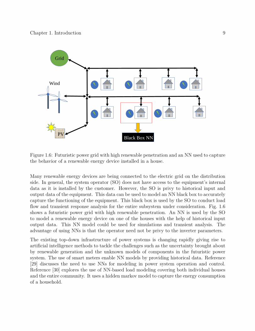
Figure 1.6: Futuristic power grid with high renewable penetration and an NN used to capturethe behavior of a renewable energy device installed in a house.
Many renewable energy devices are being connected to the electric grid on the distributionside. In general, the system operator (SO) does not have access to the equipment’s internaldata as it is installed by the customer. However, the SO is privy to historical input andoutput data of the equipment. This data can be used to model an NN black box to accuratelycapture the functioning of the equipment. This black box is used by the SO to conduct loadflow and transient response analysis for the entire subsystem under consideration. Fig. 1.6shows a futuristic power grid with high renewable penetration. An NN is used by the SOto model a renewable energy device on one of the houses with the help of historical inputoutput data. This NN model could be used for simulations and transient analysis. Theadvantage of using NNs is that the operator need not be privy to the inverter parameters.
The existing top-down infrastructure of power systems is changing rapidly giving rise toartificial intelligence methods to tackle the challenges such as the uncertainty brought aboutby renewable generation and the unknown models of components in the futuristic powersystem. The use of smart meters enable NN models by providing historical data. Reference[29] discusses the need to use NNs for modeling in power system operation and control.Reference [30] explores the use of NN-based load modeling covering both individual housesand the entire community. It uses a hidden markov model to capture the energy consumptionof a household.

Chapter 1. Introduction 10
1.3 NN for Cybersecurity
A cyberattack is a maneuver targeting existing infrastructures, information systems, com-puter networks, or personal devices. It attempts to obtain confidential data with maliciousintent [31]. The different cyberattacks include malware, network spoofing, corruption of sys-tem data, and destruction of physical components. Security against cyberattacks is difficultas any system has a wide attack surface due to the presence of heterogeneous components.Hence, it is bound to have undiscovered vulnerabilities increasing the potential points of at-tack [32, 33]. A robust defense against cyberattacks would employ a multipronged approachcombining various techniques. The techniques utilized can be classified as follows [34]:
• Redundancy: Redundancy entails deployment of additional components in the sys-tem to maintain normalcy in functionality. Even if some components are attacked,redundancy ensures that the overall system functions smoothly. Redundancy providesfor multiple instances of the same component. Let pc ⊂ Ic where Ic denotes the setof implementations that are utilized for component c ∈ C. Let Ti denote the costof redundancy when an instance of i ∈ pc is deployed. The cost for implementingredundancy is
Redundancy cost =∑c∈C
∑i∈pc
Ti.
Ti captures the costs related to deployment of additional instances of a component.This includes purchasing of hardware and maintenance.
• Heterogeneity: Heterogeneity entails hardware and software implementations of com-ponents. This ensures that vulnerabilities inherent in one kind of implementation donot impact the system as a whole. References [35, 36] show that software implemen-tations of a hardware component alone can be very effective at reducing the potencyof cyberattacks. Heterogeneity is modeled by choosing different implementations pc tobe deployed for each component c ∈ C. The cost for implementing heterogeneity is
Heterogeneity cost =∑c∈C
∑i∈pc
Di.
Di captures the costs associated with one hetergenous implementation of a component.This includes obtaining a software license, training people to use different implementa-tions, and maintaining them. NNs can be used to provide cybersecurity using hetero-geneity. NNs have the ability to model power system components such as a controlleror a subsystem as discussed in the previous section. This attribute of NNs could beused to provide cybersecurity for vulnerable components of the system by providingan alternate version of the same component. If the parameters of the component are
Chapter 1. Introduction 11
changed by a cyberattack, the NN black box could provide a layer of cybersecuritythrough heterogeneity. In the fourth chapter of this thesis, cybersecurity through het-erogeneity is explored for the controller of a VSC. A cyberattack on the controller ofa system, such as changing the parameters of the control action, can have a lastingimpact on the system itself. For example, reference [37] shows that an increase in pro-portional gain of a controller results in the increased risk of subsynchronous controlinteraction (SSCI). SSCI is a stability issue caused by interaction of series compensatedelectricity networks and the DFIG. This could lead to system instability by increas-ing oscillations. An attack on one controller of a wind turbine could be lucrative tocyberattackers with malicious intent.
• Hardening: Hardening entails reinforcing components with additional protectionschemes such as firewalls. This reduces the chance of the cyberattacker stumblingupon the vulnerabilities during the time of the attack. Hardening also reduces thechance of discovering vulnerabilities in a given implementation type during the cyber-attack. Hardening techniques include implementation of a code-secure policy, penetra-tion testing, and external expert verification. Let L represent all the hardening levelsfor a particular component c ∈ C The cost for implementing hardening is
Hardening cost =∑c∈C
∑l∈L
Hi.
Hi captures the costs associated with a single layer of hardening for a component. Thisincludes installing antivirus softwares and performing penetration testing.
1.4 Thesis Outline
The rest of the thesis is organized as follows:
Chapter 2: NN Custom Component in PSCAD
Chapter 2 describes the step by step development of an NN custom component inPSCAD/EMTDC software. It discusses the various parameters of this component, the ac-tivation function choices, and the procedure behind the design of the component. It delvesinto the logic behind the code providing a detailed explanation on preconditioning of weightsand biases, dimension creation, and recursive referenced calling.

Chapter 1. Introduction 12
Chapter 3: NN Emulator for a Voltage-Sourced Converter (VSC)Controller
Chapter 3 investigates the performance of an NN emulator for a VSC controller inPSCAD/EMTDC software. The emulator is trained on the keras python package and isrecreated in PSCAD using the NN custom component. The emulator is tested and performssatisfactorily for different short circuit ratios (SCR) and fault conditions.
Chapter 4: Cybersecurity in VSC
Chapter 4 discusses the benefits of using machine learning and artificial intelligence forproviding cybersecurity. It utilizes the NN emulation of a VSC controller to provide cyber-security.
Chapter 5: Submodule Fault Detection in Modular Multilevel Con-verters (MMC) using Support Vector Classification (SVC)
Chapter 5 proposes an SVC-based MMC submodule (SM) double-switch open-circuit (OC)fault diagnosis method combining detection and localization. With increasing use of MMCs,diagnosis and localization of SM faults are gaining importance. Most of the existing SMOC fault detection methods perform diagnosis and localization separately contributing tolonger detection times. The proposed method does not require any additional hardware.The training data for the SVC is created by simulating normal operation and SM double-switch OC faults in PSCAD/EMTDC software. Simulation results are provided to analyzethe performance of the proposed method.
Chapter 6: Conclusions and Future Work
Chapter 6 discusses the contributions of the thesis and explores directions for future research.Research directions include using other NNs to detect all kinds of submodule faults. Faultsdetection times can be optimized by using recurrent neural networks and LSTMs that makeuse of time series data to perform classification.

Chapter 2
NN Custom Component in PSCAD
This chapter describes the step by step development of an NN custom component (NNCC) inPSCAD/EMTDC. PSCAD/EMTDC is the de facto simulation software used for analyzingelectrical network transients. This implementation idea can be extended to other softwaresas well. With the advent of NN applications in power systems, simulating NN-based ap-plications and observing their effects assumes importance. However, there is no existingcomponent in PSCAD that can recreate an NN. It is in this context that an NNCC wasbuilt to help future researchers and engineers. The benefits of the NNCC are as follows:
1. The process of recreating an NN in PSCAD is time consuming as it involves multiplesummer blocks, multiplication blocks, and CSMF functions such as comparators. Theimplementation becomes time consuming with increase in number of hidden layers,neurons per hidden layer, and usage of complex activation functions. The NNCC,with its precompiled structure, eliminates the need to manually assemble blocks.
2. The NNCC reduces human error in entering weights and bias values by reading themfrom a text file.
2.1 Parameters of the NN Custom Component
1. Number of inputs: This parameter determines the number of inputs to the NN. TheUI designed ensures that the number of input neurons visible is equal to the numberentered in this parameter field. This is achieved through conditional statements in thecomponent definition in PSCAD.
2. Number of outputs: This parameter determines the number of outputs of the NN.The UI designed ensures that the number of output neurons visible is equal to thenumber entered in this parameter field. Fig. 2.2(a) shows the NNCC having 4 inputsand 3 outputs while fig. 2.2(b) shows the NNCC having 10 inputs and 10 outputs. Theoutputs can be displayed either as an array or individually.
3. Number of hidden layers: This parameter determines the number of hidden layers inthe NN. This feature makes it possible to create deep NNs having multiple hidden
13

Chapter 2. NN Custom Component in PSCAD 14
Figure 2.1: Parameters of the NNCC.
layers. Based on the number keyed in here, the custom component enables the user toenter the neuron count in each of the hidden layers. For example, if the user enters 3in this field, then the NNCC allows the user to enter number of neurons in the first,second, and third layers. These are NNCC parameters as well.
4. Neurons in the first hidden layer: This parameter determines the number of neuronsin the first hidden layer.
5. Neurons in the second hidden layer: This parameter determines the number of neuronsin the second hidden layer (entered if necessary). Fig. 2.3 shows the use of inequalitystatements in the conditional expression field to enable this parameter in the NNCC.
6. Neurons in the third hidden layer: This parameter determines the number of neuronsin the third hidden layer (entered if necessary).
7. Neurons in the fourth hidden layer: This parameter determines the number of neuronsin the fourth hidden layer (entered if necessary).
8. Neurons in the fifth hidden layer: This parameter determines the number of neuronsin the fifth hidden layer (entered if necessary).

Chapter 2. NN Custom Component in PSCAD 15
(a) (b)
(c) (d)
Figure 2.2: (a) NNCC with 4 inputs and 3 outputs, (b) NNCC with 10 inputs and 10 outputs,(c) NNCC with array outputs, and (d) NNCC with individual outputs.

Chapter 2. NN Custom Component in PSCAD 16
Figure 2.3: Enabling entering of neurons in the second hidden layer using conditional state-ments in the NNCC component defintion in PSCAD.
9. First activation function: This parameter determines the activation function of thefirst hidden layer. All the neurons in the first layer apply this activation after weightmultiplication and bias addition. The same procedure is followed for other layers.
10. Second activation function: This parameter determines the activation function of thesecond hidden layer (entered if necessary).
11. Third activation function: This parameter determines the activation function of thethird hidden layer (entered if necessary).
12. Fourth activation function: This parameter determines the activation function of thefourth hidden layer (entered if necessary).
13. Fifth activation function: This parameter determines the activation function of thefifth hidden layer (entered if necessary).
14. Output activation function: This parameter determines the activation function of theoutput layer.
15. Type of output display: This parameter determines the type of output display - arraydisplay (Fig. 2.2(c)) or individual display (Fig. 2.2(d)). Array display is preferredwhen outputs need to be tapped at a certain point and passed to other componentsin PSCAD. For example, if outputs 2 through 4 need to be combined as an array, thisoption could be utilized. Individual display is preferred when many of the outputsneed to utilized individually.
2.2 Activation Function Choices
The activation functions of the NNCC are as follows:

Chapter 2. NN Custom Component in PSCAD 17
−6 −4 −2 2 4 6
−4
−2
2
4
x
y
(a)
−6 −4 −2 2 4 6
−6
−4
−2
2
4
6
x
y
(b)
−6 −4 −2 2 4 6
−4
−2
2
4
x
y
(c)
−6 −4 −2 2 4 6
−4
−2
2
4
x
y
(d)
−6 −4 −2 2 4 6
2
4
6
x
y
(e)
−6 −4 −2 2 4 6
−2
2
4
6
x
y
(f)
−6 −4 −2 2 4 6
−2
2
4
6
x
y
(g)
Figure 2.4: Activation functions - (a) Binary step, (b) Linear, (c) Sigmoid, (d) Tanh, (e)Relu, (f) Leaky relu, and (g) Swish.

Chapter 2. NN Custom Component in PSCAD 18
1. Binary Step: The output of binary step activation equals 1 for inputs greater than0 and equals 0 for inputs lesser than or equal to 0 (Fig. 2.4(a)). Binary step hasan activation threshold of zero. It is mainly used for binary classifications. Themathematical formulation is
f(x) =
1, if x >= 0.
0, if x < 0.(2.1)
2. Linear: The output of linear activation is directly proportional to the weighted sum ofthe neuron inputs (Fig. 2.4(b)). The mathematical formulation is
f(x) = x (2.2)
3. Sigmoid: The output of sigmoid activation is constrained between 0 and 1 (Fig. 2.4(c)).This normalizes the output of the NN and ensures elimination of simple relationsbetween input and output. Sigmoid is one of the widely used nonlinear activationfunctions. It is also called the logistic function. An advantage of the sigmoid is thatthe slope is continuously differentiable. The mathematical formulation is
f(x) =1
1 + e−x(2.3)
4. Tanh: The output of tanh activation is constrained between −1 and 1 (Fig. 2.4(d)).This allows for negative outputs and is thus an improvement on the sigmoid. Tanh,also known as the hyperbolic tangent, is continuous and differentiable at all points. Itis zero centered and the gradients are not restricted to one direction. The mathematicalformulation is
f(x) =ex − e−x
ex + e−x. (2.4)
5. Relu: The output of relu activation is equal to the input for inputs greater than 0and is equal to 0 for inputs lesser than or equal to 0 (Fig. 2.4(e)). Relu activation hasbecome popular in the field of deep learning. The uniqueness of relu is that it doesnot activate all the neurons at the same time. Since only a certain number of neuronsget activated, the relu is computationally efficient compared to its other counterparts.The mathematical formulation is
f(x) = max(0, x). (2.5)
6. Leaky relu: The output of leaky relu activation is equal to the input for inputsgreater than 0 and is equal to 0.01 times the input for inputs lesser than or equalto 0 (Fig. 2.4(f)). The leaky relu is an improvised form of relu that has the same equa-tion for the positive quadrant but a small linear relationship for the negative quadrant.
Chapter 2. NN Custom Component in PSCAD 19
This ensures that there are no dead neurons in a given layer while maintaining theother advantages offered by the relu. The mathematical formulation is
f(x) =
x, if x >= 0.
0.01x, if x < 0.(2.6)
7. Swish: The output of swish activation is related to its input through a polynomialequation (Fig. 2.4(g)). Swish was proposed by the Google Brain Team. Unlike otheractivation functions, it is smooth and monotonic unbounded above and below. Exper-imental results show that the swish activation function performs better than relu ondeeper models across diverse and challenging data sets. The values for swish go fromnegative infinity to infinity. The mathematical formulation is
f(x) =x
1− e−x. (2.7)
2.3 NNCC Procedure
Reading the weights
and biases at T =0 s
(presimulation time)User controls
NNCC
parameters
Inputs to
NNCC
Creation of indexed
arrays for parameters
and inputs
Recreation of the
Deep Neural
Network structure
Arguments passed from PSCAD to C
Computation for the
given set of inputs,
activation functions,
hidden layers, and
number of neurons
NNCC
Outputs
Activation
functions
Hidden
Layers
Number of per
hidden neurons layer
Type of output
display
PSCAD
Canvas
Figure 2.5: NNCC procedure describing the flow of parameters and inputs from PSCAD toC and outputs from C to PSCAD.
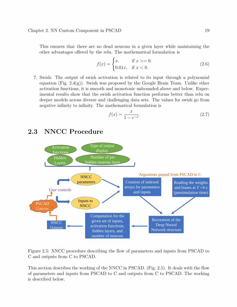
This section describes the working of the NNCC in PSCAD. (Fig. 2.5). It deals with the flowof parameters and inputs from PSCAD to C and outputs from C to PSCAD. The workingis described below.

Chapter 2. NN Custom Component in PSCAD 20
1. The NNCC reads the weights and biases at time T = 0 s as the weights do notchange during the simulation. This makes the simulation faster and more efficient.The weights and biases are obtained from a text file through a parameter passed byreference from PSCAD. Passing the parameter by value does not work as the weightsand biases are written in a different memory location leading to passing back of informalvalues.
2. The inputs and parameters of the NNCC are passed from PSCAD to C. The parametersof the NNCC include the activation functions, hidden layers, number of neurons perhidden layer, and the type of output display. The arguments (inputs and parameters)are passed as an array from PSCAD to C.
3. The NNCC C code recreates the neural network structure, computes the outputs, andreturns them to PSCAD.
2.3.1 Interfacing Challenges
1. The 1D array used to pass weights should be referenced from outside the NNCC inPSCAD. The weights cannot be read using local variables in C or inside the NNCC.The reading and passing of weights and biases throws up informal values and thesubsequent computations become wrong. In general, when arrays are passed by value,the memory locations are passed and not the values themselves.
2. The gfortan compiler compiles versions of C older than 2005. Due to this, variablescannot be initialized inside the for loop definition. They have to be predefined. Olderversions of C also require all functions called to be defined and declared before theirusage.
2.4 Logic behind Code
This section discusses the implementation of the NN in C. The inputs and the parametersare received in C as referenced arrays from PSCAD.
2.4.1 Preconditioning of Weights and Biases
The weights and biases are received as a 1D referenced array from PSCAD as PSCAD allowsarrays of one dimension. This has to separated into weight and bias tensors. Weight tensorswould have dimensions of 1,m, and n where m and n stand for the number of neurons in agiven layer and the number of neurons in the subsequent layer respectively. The bias tensorwould have dimensions of 1 and m where m stands for the number of neurons in that layer.

Chapter 2. NN Custom Component in PSCAD 21
NN
Custom
ComponentReferenced
parameters
as arrays
Inputs To CPre-preparation of
the read weights and
biases as tensors (3D)
after initialization
Creating the
dimensions to be used
in layer computations
Recursive referenced
calling of defined
computation functions
Layer to Layer input
traversal function
Bias Inclusion
function
Activation function
application
Storing the outputs
from the tensor onto
the referenced return
array
Layer Number > Limit
To P
SC
AD
Figure 2.6: Creation of the NN in C.
2.4.2 Dimension Creation
The number of inputs, outputs, and hidden layers are passed from the NNCC in PSCAD toC. These are rearranged as an array where each index stands for the number of neurons inthat layer. This array is important to make the code generic to any number of layers and ispassed to the three recursive functions that recreate the NN.
2.4.3 Recursive Referenced Calling
This forms the base of the NN computation. It repeatedly calls the following functions:
1. Layer to layer input traversal function
2. Bias inclusion function
3. Activation application function
A temporary referenced tensor is passed to each of the functions and the functions writetheir respective outputs in the tensor saving up memory and reducing computation time. Tothe layer to layer input traversal function, it passes the inputs to that layer as the temporary

Chapter 2. NN Custom Component in PSCAD 22
referenced tensor, the weights between the given layer and the next layer as a matrix, andthe dimensions of the current layer and the subsequent layer. The output tensor after weightmultiplication is returned back to the recursive referenced calling block. To the bias inclusionfunction, it passes the outputs of that layer as a temporary referenced tensor and the biases tobe added to that layer as an array. The output tensor after bias implementation is receivedby the recursive referenced calling block. It passes the outputs tensor and the choice ofactivation function for that layer to the activation application function. The output tensor,after application of the activation function, is returned to the recursive referenced callingblock. When the limit reaches the number of layers, the tensor outputs are written onto a1D array that will be sent back into PSCAD.
2.5 Preparation of Weights and Biases
This section discusses the preparation of weights and biases for the NNCC. The weights andbiases are fed in the form of a text file (.txt extension). The entries can be either integer orfloat. All the weights should be entered first followed by the biases. Each entry should beseparated from the next entry either by a single space (Fig. 2.7), a tab space (Fig. 2.9), aline (Fig. 2.8), or any combination of the above.
Figure 2.7: Preparation of weights and biases (single space format).

Chapter 2. NN Custom Component in PSCAD 23
Figure 2.8: Preparation of weights and biases (line format).
Figure 2.9: Preparation of weights and biases (tab format).

Chapter 3
NN Emulator for VSC Controller
The introduction of PV, wind energy systems, and battery storage systems along with con-trol, protection, and communication provide the bedrock to building a smarter power grid[38]. Within this new framework, power electronics is key because of its omnipresence rightfrom generation and distribution to applications involving AC and DC systems [39]. Powerelectronic devices such as the VSC are put to use in both HVDC transmission and FACTS[40]. STATCOM, which is a FACTS device, uses VSCs to provide reactive power [41]. Var-ious controllers are used to control VSCs. PI controllers [42] are widely applied in controlsystems used in the industry because of the small number of parameters to be tuned [43]. PIcontrollers eliminate the steady state error in response to a step change in the reference. In-ternal model control (IMC) is an alternative to the traditional control methods. The idea ofthe IMC is to utilize the advantages of both the feedforward and feedback control methods.IMC provides a superior control performance [44] over conventional PI by providing a fasterstep response, less overshoot in transient response, higher axes decoupling and robustnessagainst faults. Due to the importance of the controller in a VSC, an NN emulator is exploredfor the same.
This chapter proposes and analyzes the implementation and performance of an online NNcontroller emulator for VSCs. The performance of the NN emulator is investigated understep changes in the input reference values, different fault conditions, and different SCRs.This chapter is structured as follows: Section 3.1 provides a detailed insight into the im-plementation aspects of the NN controller emulator. Simulation results are provided anddiscussed in Section 3.2 and conclusions are provided in Section 3.3.
3.1 Implementation of the NN Controller Emulator
This section provides an insight into the implementation of the NN controller emulator. TheNN emulator is trained to predict the terminal voltage of the VSC given the reference valuesof the direct and quadrature axes currents. The training data is obtained from the behaviorof the IMC controller against different set points using PSCAD/EMTDC software.
24

Chapter 3. NN Emulator for VSC Controller 25
3.1.1 Importance of Data Scaling
Data scaling is critical step in preconditioning the data. Proper scaling distinguishes a goodmodel from a weak one. The commonly used data scaling techniques are standardizationand normalization. Normalization bounds the data values between two numbers whereasstandardization transforms the data to have a mean of 0 and a variance of 1 making thedata unitless. Neural networks operate on numbers without any knowledge of what thatnumber represents. In this process, they make an assumption that features with higherranging numbers are more important than their counterparts. This affects the weight thatthe NN assigns to the feature. The benefits of data scaling are as follows:
1. Assignment of equal footing to every feature before training.
2. Faster convergence of weight updation algorithms like the gradient descent.
3. Prevention of saturation in activation functions.
Min-max scaler, standard scaler, max-absolute scaler, and power-transformer scaler are a fewdata scaling techniques that are widely used. The min-max scaler performs transformationby scaling the features to a given range on the training set. It responds well when thedistribution is not gaussian. As the controller training data is not gaussian, the min-maxscaler works well.
3.1.2 Building the Model
The NN emulator model type is dense and sequential. The model has 1 hidden layer com-prising 10 neurons, 2 inputs, and 2 outputs. Increasing the number of neurons in each layerincreases model capacity which, in turn, improves accuracy. The model stops improvingafter a certain point. Generally, the more the training data provided, the larger the modelshould be [45]. The NN capacity increases with more hidden layers. At the same time, thisincreases the chance of overfitting. As a good rule of thumb, the number of hidden layersshould be
1. 0: When the data is linearly separable.
2. 1: When the data is mappable from one continuous finite space to another.
3. ≥ 2: When the data is a time series or a convolution of 2 mathematical functions.
Thus, an online NN controller emulator would need one hidden layer to map continuous databetween the input and output spaces.

Chapter 3. NN Emulator for VSC Controller 26
Relu is chosen as the activation function of the hidden layer. Although it is two linear pieces,it works well in the NN emulator due to its faster convergence. Linearity ensures that theoutput of the neuron does not plateau when the output of the neuron gets large.
3.1.3 Compiling the Model
The two parameters required to compile the model are the type of optimizer and the lossfunction. The optimizer controls the learning rate. The NN emulator uses the adam opti-mizer. Adam is a combination of stochastic gradient descent with momentum and RMSprop.Like RMSprop, it uses the squared gradients while adjusting the rate of learning. It usesthe moving average of the gradient instead of the gradient value itself. The learning ratedetermines the time required to optimize the weights for the model. The loss function usedis the mean squared error. It is computed by obtaining the average of the squared differencebetween the actual and predicted values. The model performs better when the mean squarederror is close to zero.
3.1.4 Training the Model
Four parameters are required to train the NN controller emulator: training data, targetdata, validation split, and the number of epochs. For each epoch, the model cycles throughthe entire training data. The number of epochs used in the NN controller emulator is 100.The more epochs the data is cycled through, the greater the improvement in the model upto a certain point. Table 3.1 shows the behavior of mean absolute error (MAE) and theloss as the NN emulator cycles through the training data. An increase in the number ofepochs increases the runtime. A good estimate for number of epochs is to stop when theuser observes the error converging at a fixed value. If the converging error value is high, thenit is recommended to increase the number of layers or the number of neurons. It should benoted that there is no one particular solution to this issue.
Table 3.1: Behavior of mean absolute error (MAE) and loss function as the NN emulatorcycles through the training data.
Epoch number Loss MAE1 0.0095 0.03392 3.7553× 10⁻⁵ 0.00463 3.7535× 10⁻⁵ 0.0046

Chapter 3. NN Emulator for VSC Controller 27
(a) (b)
Figure 3.1: (a) id tracking by the NN emulator for step changes in id ref and (b) iq trackingby the NN emulator for step changes in id ref.
3.2 Performance Evaluation
The NN emulator model is built in PSCAD/EMTDC software after it is trained using thekeras python package. Four case studies, for which the NN is not trained, are used toevaluate its performance. They are discussed below.
3.2.1 Step Change in Direct Axis Current Reference
The direct axis current reference id ref is changed from 0.02 pu to 0.372 pu at t = 0.4 s andback to 0.02 pu at t = 0.5 s. Fig. 3.1(a) shows the successful tracking of id to step changesin id ref. Fig. 3.1(b) shows the successful tracking of iq to step changes in id ref. The NNemulator has a settling time of 0.02 s while the IMC controller has a comparable settlingtime of 0.01 s.
3.2.2 Step Change in Quadratic Axis Reference
The quadrature axis current reference iq ref is changed from 0.02 pu to 0.55 pu at t = 0.55 sand back to 0.02 pu at t = 0.60 s. Fig. 3.2(a) shows the successful tracking of iq to stepchanges in iq ref. Fig. 3.2(b) shows the successful tracking of id to step changes in iq ref. TheNN emulator has a settling time of 0.009 s while the IMC controller has a comparable settlingtime of 0.006 s.
3.2.3 Single-Phase to Ground Fault at PCC
A single-phase AG fault is simulated at t = 0.4 s for 0.05 s at PCC. The NN emulatorcontinues to track id ref after the fault is cleared and does not lose stability (Fig. 3.3).

Chapter 3. NN Emulator for VSC Controller 28
(a) (b)
Figure 3.2: (a) iq tracking by the NN emulator for step changes in iq ref and (b) id trackingby the NN emulator for step changes in iq ref.
Figure 3.3: id tracking by the NN emulator for a single-phase AG fault at the PCC.
3.2.4 Increasing SCR by a Factor of 10
The SCR of the system is increased by a factor of 10. id ref is changed to 0.42 pu from 0.02 puat t = 0.55 s and back to 0.02 pu at t = 0.60 s. Fig. 3.4 shows the successful tracking of idto step changes in id ref.
3.3 Conclusions
This chapter studies the performance of NN controller emulator for a VSC. Both the NNemulator and the controller are modeled in PSCAD/EMTDC software. The emulator istested for four scenarios and performs satisfactorily. Further, this controller emulator canbe useful to detect and mitigate cyberattacks on the controller itself.

Chapter 3. NN Emulator for VSC Controller 29
Figure 3.4: id tracking by the NN emulator for a change in the SCR.

Chapter 4
Cybersecurity in VSC
The smart grid is an improvement over traditional power system infrastructure [46]. Powersystem topology is predominantly centralized and radial. This is changing with the adventof smart grids. Unidirectional power flow solutions are becoming invalid with increasedrenewable penetration from the consumer end. This requires new strategies in protection,control, and communication [47]. A smart grid system consists of many VSCs which coex-ist with synchronous generators. Some basic communication is required between the VSCsto perform grid functions. VSC control is of two types: centralized and decentralized. Incentralized control, all the VSCs correspond with a central entity that processes the dataobtained from the VSCs, calculates the task that each VSC has to do, and communicatesthe same to the VSCs. In such a scenario, data flows from bottom (VSC) to top (centralizedcontroller) while commands flow from top (centralized controller) to bottom (VSC). Thismakes the centralized architecture vulnerable to cyberattacks as it is prone to single point offailure. The SCADA system is a pertinent example of centralized control. A potential issuein centralized control is the quantum of communication resources required as the number ofVSCs in the system increase. VSCs that are geographically far apart and may have no bear-ing on each other would be required to communicate with the same centralized controller toobtain their set points. In contrast, decentralized control offers a solution to these problems.As the name suggests, it is decentralized in its control paradigm as computational resourcesare distributed across the power system rather than being concentrated. This ensures thatlow bandwidth communication is sufficient to meet the requirements driving down cost.In this control approach, only local and highly relevant measurements are utilized. Thisapproach has its limitations as well. Cyberattacks can be formulated capitalizing on insuffi-cient information present at a particular node [48]. The changing trends in the way power isgenerated (renewable energy, energy storage), transmitted (storage as a transmission assetamong other things), and distributed has contributed to the need for a robust cybersecurityapproach to combat cyberattacks that strive to throw the power grid off its operation fornumerous reasons including monetary benefits.
This chapter proposes and investigates an NN-based cybersecurity approach for VSCs. VSCshave become increasingly popular with the ability to provide frequency and voltage supportto the grid. Like other components of the grid, the VSC has become prone to cyberattacks.
This chapter is structured as follows: Section 4.1 provides an insight into the VSC andthe differential equations governing it. Section 4.2 provides an overview of using AI for
30
Chapter 4. Cybersecurity in VSC 31
abc/dqi3ϕo idqo Current Control
idq∗o
u∗dq PWM
+
−vdc
idc io
PCC
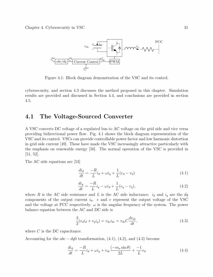
Figure 4.1: Block diagram demonstration of the VSC and its control.
cybersecurity, and section 4.3 discusses the method proposed in this chapter. Simulationresults are provided and discussed in Section 4.4, and conclusions are provided in section4.5.
4.1 The Voltage-Sourced Converter
A VSC converts DC voltage of a regulated bus to AC voltage on the grid side and vice versaproviding bidirectional power flow. Fig. 4.1 shows the block diagram representation of theVSC and its control. VSCs can provide controllable power factor and low harmonic distortionin grid side current [49]. These have made the VSC increasingly attractive particularly withthe emphasis on renewable energy [50]. The normal operation of the VSC is provided in[51, 52].
The AC side equations are [53]
diddt
=−R
Lid + ωiq +
1
L(ed − vd) (4.1)
diqdt
=−R
Liq − ωid +
1
L(eq − vq), (4.2)
where R is the AC side resistance and L is the AC side inductance. id and iq are the dqcomponents of the output current i0. e and v represent the output voltage of the VSCand the voltage at PCC respectively. ω is the angular frequency of the system. The powerbalance equation between the AC and DC side is
3
2(edid + eqiq) = vdcidc = vdcC
dvdcdt
, (4.3)
where C is the DC capacitance.
Accounting for the abc− dq0 transformation, (4.1), (4.2), and (4.3) become
diddt
=−R
Lid + ωiq + vdc
(−ma sin θ)
2L+
−1
Lvd (4.4)

Chapter 4. Cybersecurity in VSC 32
diqdt
=−R
Liq − ωid + vdc
(ma cos θ)2L
+−1
Lvq (4.5)
dvdcdt
=(−3ma sin θ)
4Cid +
(3ma cos θ)4C
iq (4.6)
where ma is the modulation index and θ = ωt (t is time). Equations (4.4), (4.5), and (4.6)are put in state space representation dx
dt= Ax + Bu where x = (id, iq, vdc) and u = (vd, vq)
in order to obtain the governing ODE of the system. The state space matrices are
A =
−RL
ω −ma sin θ2L
−ω −RL
ma cos θ2L
−3ma sin θ4C
3ma cos θ4C
0
and
B =
−1L
0
0 −1L
0 0
4.2 AI and Cybersecurity
Cybersecurity, in the past, has been a combination of hardware, software, and common sensehuman intervention approaches. Artificial intelligence (AI) can help combat cyberattacks byproviding component heterogeneity. As malicious attacks have grown in novelty, they havelearned to camouflage better. They can change their own code making it difficult for theexisting cybersecurity approaches to detect them. AI-based cybersecurity can however helpin identifying such patterns being introduced to the network under consideration. RecurrentNNs (RNN) can be used to identify the temporal behavior of an attack. This is usefulin detecting and mitigating similar attacks in the future. Some of the benefits of AI forcybersecurity include
1. Handling volume: AI can obtain and analyze large volume of activity in a small fractionof time required by other resources. It can help filter benign material freeing up otherresources to focus on the small subset of the data containing suspected activity.
Chapter 4. Cybersecurity in VSC 33
2. Ability to learn with time: AI can identify cyberattacks based on its interaction withsimilar attacks in the past.
3. Identifying unknown threats: AI can spot deviations from the norm. This featurecan be put to use in identifying unknown scenarios that may turn out to be potentialthreats.
On the other hand, AI only accelerates processes humans can do. Though powerful, AI isrelatively new to cybersecurity and has its limitations. The limitations of AI include
1. Continuous evolution of cyberthreats: Cyberthreats are continuously evolving. Cyber-attackers have access to unlimited resources and solutions that require AI would needto be constantly updated.
2. Use of AI by attackers: When the AI based cybersecurity solution becomes widelyavailable, attackers can make use of it to formulate a malware strain that is unaffectedby the AI-based cybersecurity apparatus. They can use the same machine learningtechniques to disguise the attack. Another scenario to be considered is the pollutionof training data which leads to the entire cyber apparatus being compromised.
AI-based cybersecurity techniques are increasingly used as the first line of defense savinghuman analysts a lot of time.
4.3 Proposed Method
The NN has been used for cybersecurity applications such as intrusion detection and pre-vention systems [54], combating malware [55], and network traffic analysis [56]. An NN canmimic the system it is asked to learn and be used like state estimators to substitute forparameters whose values are compromised by the attack. This estimate would be close tothe accurate value and can ensure smooth functioning of the system despite the cyberattack.This cybersecurity approach is also called cybersecurity through heterogeneity.
An NN-cybersecurity apparatus is used to protect the VSC against attacks on its controller(Fig. 4.1). The NN emulates the VSC controller. The controller outputs ud and uq are usedto generate the PWM signals that fire the VSC. Any tampering of this signal affects thestate variables id and iq of the VSC and leads to forced changes to the operating modulationindex and the power output of the VSC. This would disturb its power sharing arrangementswith other generators (conventional and VSC). At its worst, it would lead to high currentsresulting in damage to power electronic equipment. This can trip the inverter from the gridand lead to its shutdown. The cyberattack can be easily carried out through the help of amalware. A malware is used to describe any vicious software designed to cause intentional

Chapter 4. Cybersecurity in VSC 34
Input Layer
Hidden Layer
Output Layer
id id ref iq iq ref
ud uq
Figure 4.2: Proposed NN for cybersecurity.
damage to any network. Types of malware include virus, worms, trojans, spyware, andransomware. It enters the system through a random node in a compromised network. Then,it traverses through the network compromising more nodes in its path till it decides to launchan attack [57].
The VSC system considered in this chapter can be thought of as a node that is compromisedby a simple malware. An online NN can provide cybersecurity for the VSC controller. Thetraining data is obtained by simulating the VSC and controller system in PSCAD/EMTDCsoftware. The inputs to the NN are the measured current values and their respective ref-erences. The structure of this NN is shown in Fig. 4.2. The VSC parameters are listed inTable 4.1 and controller parameters are listed in Table 4.2. The NN is trained to predict ud
and uq which are fed to the PWM to generate the firing signals.
The NN comprises one hidden layer consisting of 10 neurons. A single hidden layer is used indesigning the controller as the function maps continuous data from the input space to outputspace. The relu activation function [58] is used as it does not suffer the vanishing gradientproblem. Adam optimization [59] is utilized as it provides the benefits of both stochasticgradient and RMSprop [59]. The loss function used for updating the weights is the meansquared error.
Chapter 4. Cybersecurity in VSC 35
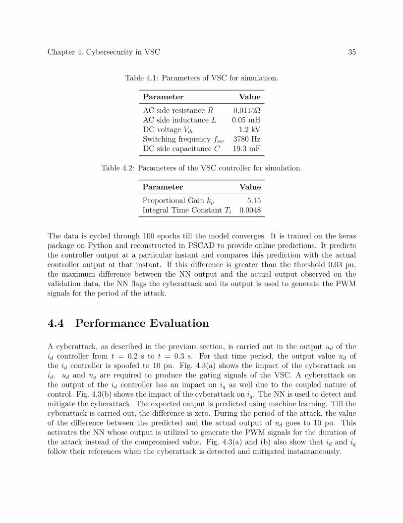
Table 4.1: Parameters of VSC for simulation.
Parameter ValueAC side resistance R 0.0115ΩAC side inductance L 0.05 mHDC voltage Vdc 1.2 kVSwitching frequency fsw 3780 HzDC side capacitance C 19.3 mF
Table 4.2: Parameters of the VSC controller for simulation.
Parameter ValueProportional Gain kp 5.15Integral Time Constant Ti 0.0048
The data is cycled through 100 epochs till the model converges. It is trained on the keraspackage on Python and reconstructed in PSCAD to provide online predictions. It predictsthe controller output at a particular instant and compares this prediction with the actualcontroller output at that instant. If this difference is greater than the threshold 0.03 pu,the maximum difference between the NN output and the actual output observed on thevalidation data, the NN flags the cyberattack and its output is used to generate the PWMsignals for the period of the attack.
4.4 Performance Evaluation
A cyberattack, as described in the previous section, is carried out in the output ud of theid controller from t = 0.2 s to t = 0.3 s. For that time period, the output value ud ofthe id controller is spoofed to 10 pu. Fig. 4.3(a) shows the impact of the cyberattack onid. ud and uq are required to produce the gating signals of the VSC. A cyberattack onthe output of the id controller has an impact on iq as well due to the coupled nature ofcontrol. Fig. 4.3(b) shows the impact of the cyberattack on iq. The NN is used to detect andmitigate the cyberattack. The expected output is predicted using machine learning. Till thecyberattack is carried out, the difference is zero. During the period of the attack, the valueof the difference between the predicted and the actual output of ud goes to 10 pu. Thisactivates the NN whose output is utilized to generate the PWM signals for the duration ofthe attack instead of the compromised value. Fig. 4.3(a) and (b) also show that id and iqfollow their references when the cyberattack is detected and mitigated instantaneously.

Chapter 4. Cybersecurity in VSC 36
4.5 Conclusions
This chapter studies NN cybersecurity through heterogeneity. Both the NN and the VSCsystem are modeled in PSCAD/EMTDC software. The NN is able to effectively detect andmitigate the cyberattacks on the VSC controller by emulating it. Cybersecurity throughheterogeneity can be extended to a multiinverter microgrid setup as well. Machine learningand artificial intelligence could supplement the existing cybersecurity apparatus reducinghuman intervention and increasing overall efficacy.
Chapter 4. Cybersecurity in VSC 37
(a)
(b)
Figure 4.3: (a) id behavior during cyberattack on id controller output and when the attackis detected and mitigated and (b) iq behavior during cyberattack on id controller output andwhen the attack is detected and mitigated.

Chapter 5
Submodule Fault Detection in MMCsusing Support Vector Classification
This chapter proposes a support vector classifier (SVC)–based SM double-switch OC faultdiagnosis method, combining detection and localization. With increasing use of modularmultilevel converters (MMC), diagnosis and localization of submodule (SM) faults are gainingimportance. Most of the existing SM open-circuit (OC) fault detection methods performdiagnosis and localization separately leading to longer detection times. The proposed methoddoes not require any additional hardware. The training data for the SVC is created bysimulating normal operation and SM double-switch OC faults in PSCAD/EMTDC software.Simulation results analyze the performance of the proposed method.
5.1 Introduction
The modular multilevel converter (MMC) is a power electronics converter topology used inHVDC power transmission, FACTS devices, and high-voltage drives. The MMC can helpgenerate high voltage levels with low harmonic content through low voltage SMs which canbe controlled individually [60]. Some of the advantages of the MMC are as follows:
1. Good output harmonic performance when providing high voltages [60],
2. High modularity [61], and
3. Low current rating for power switches [60].
An MMC consists of many SMs and each SM contains insulated gate bipolar transistors(IGBT). IGBTs are one of the most fragile components in the SM, making them prone tofiring faults [62], [63]. These faults can be classified as open-circuit (OC) and short-circuit(SC). SMs typically have SC withstand times in the order of microseconds as the capacitorin the SM discharges immediately [64]. SM SC faults are suppressed by hardware diagnosticmethods [65], [66]. However, SM OC faults can remain undetected without specific diagnosticmethods, lead to derating of the MMC by preventing discharge of the capacitor in thefaulted SM. This damages the converter [67] and distorts the current waveform [68]. Proper
38
Chapter 5. Submodule Fault Detection in MMCs using Support Vector Classification 39
diagnosis of the SM OC fault requires fault detection and localization. Fault detectionmethods generate an alarm to indicate the occurrence of an OC switch fault in a phase.The faulty SMs are identified through fault localization methods and bypassed by theirantiparallel switches using a fault-tolerant control method.
SM OC fault detection methods can be of two types: hardware-based and software-based [69].Reference [70] proposes a hardware-based nearest level modulation (NLM) method for de-tecting OC faults. This, however, requires installation of an additional inductor winding tomeasure the voltage across the arm inductors. Reference [71] proposes a hardware-basedmethod that performs fault diagnosis in the respective SM. This method requires the mea-suring points of the voltage sensor to be reconfigured to monitor the SM terminal voltage.Reference [72] compares the output voltage of a group of SMs with certain reference volt-ages and requires an additional supervisory sensor to obtain those references. Reference [73]proposes hardware-based fault detection by studying the output voltages of the SM underboth normal and fault conditions. However, it requires the aid of an extra hardware circuitto detect SM output voltage. Hardware-based methods, in general, require changes in theinstallation, increasing the difficulty of implementation. This shortcoming reduces their ap-plicability in existing commercial projects. On the other hand, software-based fault detectionmethods proposed in [74, 75] eliminate the need for extra hardware devices. Model-basedsoftware methods compare measured state variables with estimated state variables, which arecomputed using mathematical modeling [74]. Reference [74] estimates the ideal circulatingcurrent and the output current using the state model of the MMC and the variables in themain control system. However, there is a long time interval (more than 100 ms) to diagnosewhich SM is faulty. References [76] and [77] propose data driven methods for faulty SMidentification. However, they use manually determined thresholds requiring intervention intuning. Reference [78] proposes an artificial neural network (ANN)–based method to detectthe faulted SM. This method computes a threshold for identifying how long a faulted SMexhibits highest voltage in a given time period.
This work proposes an SVC-based SM fault detection method for MMCs. The proposedmethod does not require extra hardware devices, utilizes the voltage sorting array in theMMC controller allowing it to be embedded as a code inside the controller itself. Thisremoves the need for a design change of the controller. The SVC does not require model-based state estimation and indicates the presence of a double-switch SM OC fault. Studiesare performed in PSCAD/EMTDC software to create a dataset for training the SVC. Athree-phase MMC with 4 SMs in each arm is modeled in PSCAD/EMTDC.
The rest of this work is organized as follows. Basics of MMC control, operating principlesand double-switch faults in the MMC are introduced in Section 5.2. Section 5.3 discussesthe proposed fault detection and localization method. Section 5.4 discusses the performancevalidation of the proposed method in PSCAD/EMTDC. Finally, the conclusions are providedin Section 5.5.
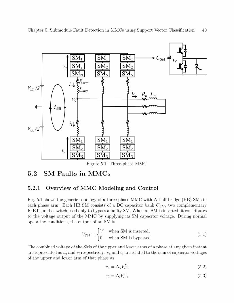
Chapter 5. Submodule Fault Detection in MMCs using Support Vector Classification 40
N
u
l
u
l
o
o
dc
arm
arm
o o
dc
1
2
SM
N
2
N
1
2
N
1
2
N
1
2
N
1
2
c
1
diff
Figure 5.1: Three-phase MMC.
5.2 SM Faults in MMCs
5.2.1 Overview of MMC Modeling and Control
Fig. 5.1 shows the generic topology of a three-phase MMC with N half-bridge (HB) SMs ineach phase arm. Each HB SM consists of a DC capacitor bank CSM , two complementaryIGBTs, and a switch used only to bypass a faulty SM. When an SM is inserted, it contributesto the voltage output of the MMC by supplying its SM capacitor voltage. During normaloperating conditions, the output of an SM is
VSM =
Vc when SM is inserted,0 when SM is bypassed.
(5.1)
The combined voltage of the SMs of the upper and lower arms of a phase at any given instantare represented as vu and vl respectively. vu and vl are related to the sum of capacitor voltagesof the upper and lower arm of that phase as
vu = NuVΣcu, (5.2)
vl = NlVΣcl , (5.3)

Chapter 5. Submodule Fault Detection in MMCs using Support Vector Classification 41
where
Nu, Nl ∈0,
1
N,2
N, . . . , 1
. (5.4)
Nu and Nl are the upper and lower arm insertion indices, and V Σcu and V Σ
cl are the sum of theSM capacitor voltages in the upper and lower arm of that phase. The single-phase equationsof an MMC are
Rarmiu + Larmdiudt
=Vdc
2− vo − vu, (5.5)
Rarmil + Larmdildt
=Vdc
2+ vo − vl, (5.6)
iu = idiff +io2, (5.7)
il =io2− idiff, (5.8)
where vo and io represent the phase to neutral output voltage and the output current, idiffthe circulating current of that phase, Vdc the dc linking voltage, vu, iu, and vl, il the voltageand current of the upper and lower arms respectively, and Larm, Rarm the arm inductanceand arm resistance respectively. Substituting (5.7) and (5.8) in (5.5) and (5.6), the ac anddc dynamic equations are as follows:
vo = −1
2
(Rarmio + Larm
diodt
)+
vl − vu2
, (5.9)
Vdc = vu + vl + 2
(Rarmidiff + Larm
didiff
dt
). (5.10)
The differential voltage, causing the differential current, is
vdiff = Vdc − vu − vl. (5.11)
The full dynamic model of the MMC for phase i is obtained from (5.2), (5.3), (5.10), and(5.11) as
didiff,i
dt=
1
2Larmvdiff,i −
Rarm
Larmidiff,i
dV Σcu,i
dt=
NNu,i
CSMiu,i
dV Σcl,i
dt=
NNl,i
CSMil,i,
(5.12)
where CSM is the SM capacitance.
MMC control is performed using selective harmonic elimination pulse width modulation(SHE-PWM) proposed in [79]. Fig. 5.2 shows the MMC controller used for this analysis. Ittracks the circulating current reference idiff, maintains the averaged voltage of SM capacitorsand limits the idiff ripple.
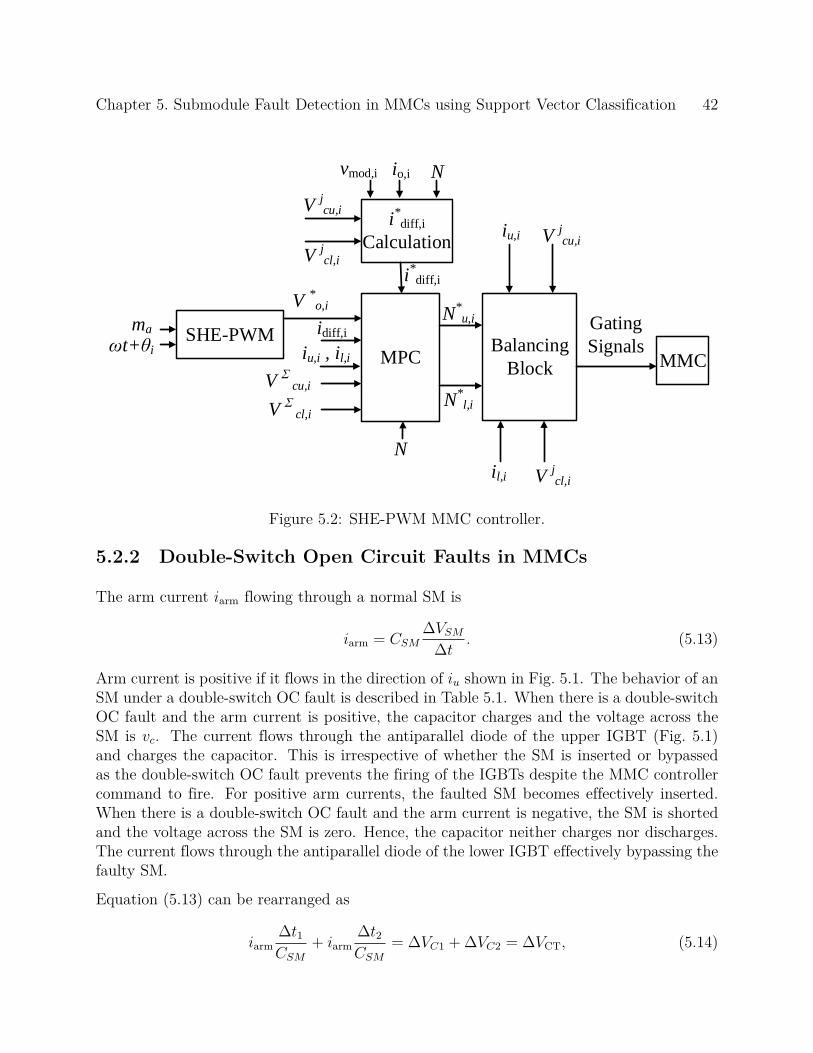
Chapter 5. Submodule Fault Detection in MMCs using Support Vector Classification 42
SHE-PWMma
ωt+θi
idiff,i
V jcu,i
MPC
V *o,i
i*diff,i
i*diff,i
Calculation
Nio,ivmod,i
V jcl,i
V Σ
cu,i
V Σ
cl,i
iu,i , il,i
N
N*l,i
N*u,i
Balancing
Block MMC
Gating
Signals
iu,i
il,i
V jcu,i
V jcl,i
Figure 5.2: SHE-PWM MMC controller.
5.2.2 Double-Switch Open Circuit Faults in MMCs
The arm current iarm flowing through a normal SM is
iarm = CSM∆VSM
∆t. (5.13)
Arm current is positive if it flows in the direction of iu shown in Fig. 5.1. The behavior of anSM under a double-switch OC fault is described in Table 5.1. When there is a double-switchOC fault and the arm current is positive, the capacitor charges and the voltage across theSM is vc. The current flows through the antiparallel diode of the upper IGBT (Fig. 5.1)and charges the capacitor. This is irrespective of whether the SM is inserted or bypassedas the double-switch OC fault prevents the firing of the IGBTs despite the MMC controllercommand to fire. For positive arm currents, the faulted SM becomes effectively inserted.When there is a double-switch OC fault and the arm current is negative, the SM is shortedand the voltage across the SM is zero. Hence, the capacitor neither charges nor discharges.The current flows through the antiparallel diode of the lower IGBT effectively bypassing thefaulty SM.
Equation (5.13) can be rearranged as
iarm∆t1CSM
+ iarm∆t2CSM
= ∆VC1 +∆VC2 = ∆VCT, (5.14)
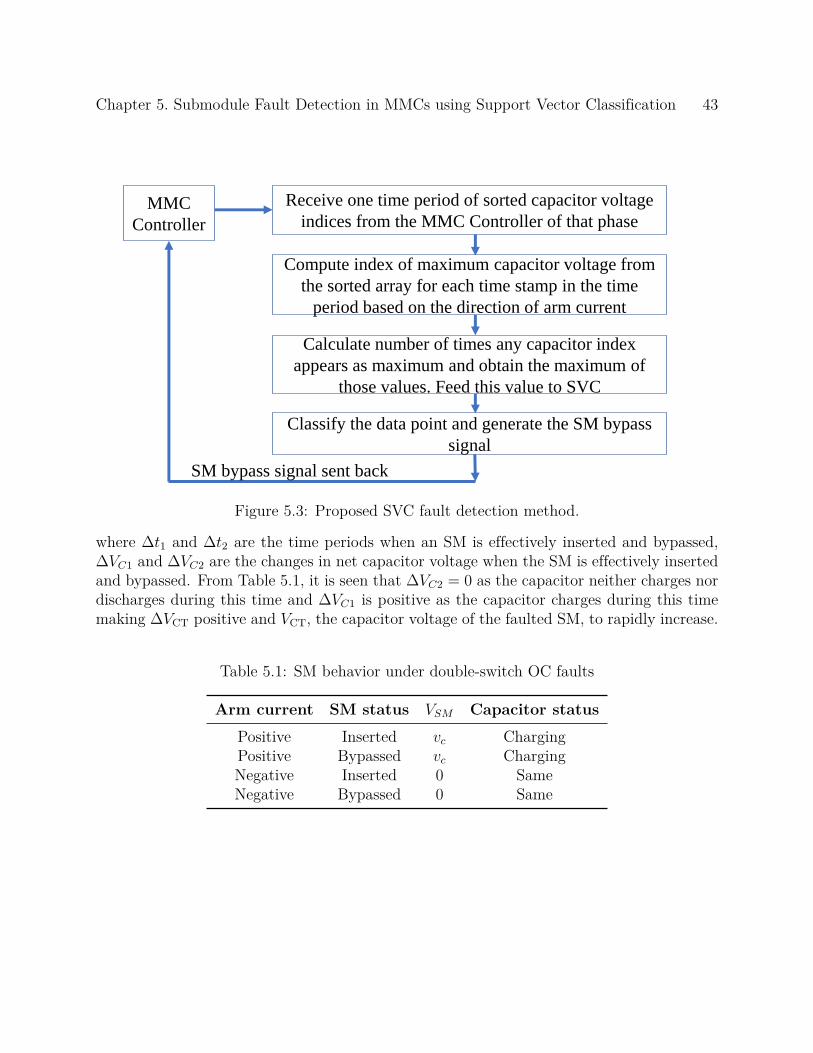
Chapter 5. Submodule Fault Detection in MMCs using Support Vector Classification 43
SM bypass signal sent back
Receive one time period of sorted capacitor voltage
indices from the MMC Controller of that phase
Compute index of maximum capacitor voltage from
the sorted array for each time stamp in the time
period based on the direction of arm current
Calculate number of times any capacitor index
appears as maximum and obtain the maximum of
those values. Feed this value to SVC
MMC
Controller
Classify the data point and generate the SM bypass
signal
Figure 5.3: Proposed SVC fault detection method.
where ∆t1 and ∆t2 are the time periods when an SM is effectively inserted and bypassed,∆VC1 and ∆VC2 are the changes in net capacitor voltage when the SM is effectively insertedand bypassed. From Table 5.1, it is seen that ∆VC2 = 0 as the capacitor neither charges nordischarges during this time and ∆VC1 is positive as the capacitor charges during this timemaking ∆VCT positive and VCT, the capacitor voltage of the faulted SM, to rapidly increase.
Table 5.1: SM behavior under double-switch OC faults
Arm current SM status VSM Capacitor statusPositive Inserted vc ChargingPositive Bypassed vc ChargingNegative Inserted 0 SameNegative Bypassed 0 Same

Chapter 5. Submodule Fault Detection in MMCs using Support Vector Classification 44
5.3 Proposed SM Fault Detection Method
5.3.1 SVC-Based Fault Detection Method
The SHE-PWM controller creates a sorted array of SM capacitor voltages for its own com-putations. The same resource is utilized to perform fault detection. Fig. 5.3 shows theproposed SVC fault detection method. The method first obtains the array of sorted SMcapacitor voltages from the MMC controller of the corresponding phase for one time pe-riod. The simulation time step is 50 µs and each time period is 0.0167 s (system frequencyis 60 Hz). This results in 334 sorted SM capacitor voltage time stamps per time period.Training data is obtained from PSCAD by simulating ten cycles each of normal and faultedoperation of SM1 in the upper arm of phase a. The number of times voltage of the SMconsidered for training VCSM1
is maximum in every time period is computed. This serves asthe training data for the SVC. The training data does not require more than two faulted SMoperation time periods as the number of times VCSM1
is maximum in a time period saturatesat 334 providing no additional information. Fig. 5.4 shows the data used to train the SVC.
After receiving one time period (334 time stamps) of sorted capacitor voltage indices from theMMC controller, the proposed method computes the index of maximum capacitor voltagefrom the sorted array for each time stamp based on the direction of arm current. If thearm current is positive, the array received from the MMC controller is sorted in descendingorder and the first element of the sorted array provides which SM capacitor has the maximumvoltage for that time stamp. If the arm current is negative, the array received from the MMCcontroller is sorted in ascending order and the last element of the sorted array provides whichSM capacitor has the maximum voltage for that time stamp. The proposed method thencomputes the number of times each SM capacitor voltage is maximum in that time periodand the maximum of those values is fed to the SVC. This data point is classified by the SVCas faulty or normal SM operation. Then, the proposed method returns a bypass signal thatindicates which SM is faulted. The bypass signal is an array with dimension equalling thenumber of SMs in the arm of that phase. Each element in the bypass signal array indicatesif that particular SM is faulted or not. If an SM is faulted, the bypass signal array returnsa value of 1 for the index corresponding to the faulted SM. Let any valid SVC hyperplaneclassifying the training data (Fig. 5.5) be denoted by g(x) = wTx + b. The optimal SVChyperplane classifier is computed by solving for the following expression:
minw
1
2wTw
subject to yi (w · xi + b) ≥ 1 ∀i,(5.15)
where w and b are the weight and the bias of the SVC and xi and yi are the input to theSVC and the output of the SVC. Equation (5.15) can be expressed in the Lagrangian form

Chapter 5. Submodule Fault Detection in MMCs using Support Vector Classification 45
Figure 5.4: Number of times VCSM1is maximum in a time period.
g(x) = -k
g(x) = 0
g(x) = +k
w
SM faulted
SM normal operation
Figure 5.5: Classification of sample support vectors using a hyper-plane.
as
minw,b
J(w, b, α) =1
2wTw − ΣN
i=1αidi(wTxi + b) + ΣN
i=1αi
subject to αi ≥ 1 ∀i,(5.16)
where the αs represent the Lagrangian multipliers. The lagrangian function J is minimizedfor w and b and maximized for α. At the optimum, dJ
dw= 0 and dJ
db= 0. Applying the above
conditions to (5.16), we get
w0 = ΣNi=1αidixi, ΣN
i=1αidi = 0. (5.17)
Equation (5.17) is substituted into (5.16), reorganized in the dual form, and solved for thelagrangian multipliers using QP optimization. The SVC weight w and bias b values are foundto be −1.3 and 1.091.

Chapter 5. Submodule Fault Detection in MMCs using Support Vector Classification 46
Table 5.2: Parameters of the MMC for simulation.
Parameter ValueNumber of SMs in each phase arm N 4DC-link voltage Vdc 10 kVSM capacitance CSM 4600 µFArm inductance Larm 9 mHLoad resistance Ro 12 ΩLoad inductance Lo 4 mHFundamental frequency fo 60 HzModulation index ma 0.8Sampling frequency fs 2 kHzRated Vc for normal operation 2.5 kV
5.4 Performance Evaluation
To evaluate the performance of the proposed SVC-based SM fault detection method, a de-tailed model of the three-phase MMC with 4 SMs in each arm is created in PSCAD/EMTDCsoftware. A double-switch OC fault is simulated in SM3 of the upper arm at time t = 0.7575 s.As discussed in Section II, when the arm current is positive, the faulted SM capacitor volt-ages increases and when the arm current is negative, the faulted SM becomes effectivelybypassed and the SM neither charges nor discharges during this time. Thus, the capacitorvoltage of the faulted SM increases in a stepwise fashion. Fig. 5.6(a) validates this behaviorin the faulted SM capacitor voltage. The lower arm current reduces by a smaller factor asit supplies the load after the fault of an SM in the upper arm. As the upper arm current ismuch smaller than the lower arm current, the rate of decrease of capacitor voltages of theupper arm SMs is lower than their lower counterparts. This can be observed in Fig. 5.6(a).
The SHE-PWM MMC controller maintains the sum of all capacitor voltages to Vdc. Whencapacitor voltage of SM3 Vca3 increases, the controller tries to reduce the voltage by modifyingthe PWM signal fed to SM3. This signal is, however, not processed by the SM due tothe double-switch OC fault and its capacitor voltage continues to increase. This leads toa reduction in the voltages of the other SMs to maintain the sum of all voltages to Vdc.Increase in Vca3 leads to an increase in the net impedance offered by the upper arm resultingin reduced upper arm current, Fig. 5.6(b).
The double-switch OC fault occurs at SM3 occurs at t = 0.7575 s. The method is able todetect the fault at t = 0.7575+0.0167 s = 0.7742 s where 0.016 s represents one time periodcorresponding to the system frequency of 60 Hz, Fig. 5.6(c).

Chapter 5. Submodule Fault Detection in MMCs using Support Vector Classification 47
5.5 Conclusions
A comprehensive double-switch OC SM fault detection and localization scheme is proposed inthis chapter. Capacitor voltages of double-switch OC faulted SMs differ from those of normalSMs. The proposed SVC-based method evaluates these voltage variations for diagnosingand localizing these faults. The sorted capacitor voltages from the controller are utilizedeliminating the need for any extra hardware. By being independent of system parameters,the proposed method is immune to parameter uncertainties ensuring high robustness. Theproposed method is evaluated through simulation studies conducted in PSCAD/EMTDC,and the results demonstrate that the method works accurately and efficiently.

Chapter 5. Submodule Fault Detection in MMCs using Support Vector Classification 48
(a)
(b)
Figure 5.6: (a) MMC capacitor voltages during double-switch OC faults, (b) MMC armcurrents during double-switch OC faults, and

Chapter 5. Submodule Fault Detection in MMCs using Support Vector Classification 49
(c)
Figure 5.6: (c) Bypass signal produced by the SVC.

Chapter 6
Contributions and Future Work
The contributions of the thesis are as follows:
1. Discusses the various applications of NNs in power systems.
2. Shows the step by step development of an NNCC in PSCAD/EMTDC simulationsoftware.
3. Proposes building of a NN emulator for an IMC controller of a VSC inPSCAD/EMTDC simulation software.
4. Discusses how NNs can provide cybersecurity through heterogeneity. Implementationis performed for a controller in a VSC.
5. Proposes an SVC-based algorithm to detect double-switch OC failures in the MMC.
Some avenues by which this work can be expanded in the future are as follows:
1. Addition of new features to the NNCC: The NNCC could be extended to provide addi-tional features such as enabling dropout regularization, increasing choices in activationfunctions, and enabling implementation of time dependency in NNs.
2. Exploring the use of other NNs to detect any MMC submodule fault: Support vectorclassifiers are utilized to detect double-switch OC faults by screening one time perioddata of capacitor voltage indices. RNNs, transformers, and LSTMs could be exploredto provide fault detection and localization for both single-switch as well as double-switch faults by analyzing the temporal sequence of data.
50

Bibliography
[1] “Neurons - The Computer Chip of Human Brain ,” June 2015. [Online]. Available:www.humanagingcentral.com
[2] P. Sotoodeh and R. D. Miller, “A single-phase 5-level inverter with facts capabilityusing modular multi-level converter (MMC) topology,” Intl. Elec. Mach. Driv. Conf.,May 2013.
[3] Maria Thomas, “Neural Networks: Advantages and Applications,”May 2019. [Online]. Available: https://www.marktechpost.com/2019/04/18/introduction-to-neural-networks-advantages-and-applications/
[4] Jason Brownlee, “How Much Training Data is Required for Machine Learn-ing?” May 2017. [Online]. Available: https://machinelearningmastery.com/much-training-data-required-machine-learning/
[5] Ebenezer R.H.P. Isaac, “What is the minimum sample size requiredto train a Deep Learning model - CNN?” Feb. 2016. [Online]. Avail-able: https://www.researchgate.net/post/What_is_the_minimum_sample_size_required_to_train_a_Deep_Learning_model-CNN
[6] J. Pinto, B. Bose, L. Da Silva, and M. Kazmierkowski, “A neural-network-based space-vector pwm controller for voltage-fed inverter induction motor drive,” IEEE T. Ind.Appl., vol. 36, no. 6, 2000.
[7] J. Pinto, B. Bose, and L. da Silva, “A stator-flux-oriented vector-controlled inductionmotor drive with space-vector pwm and flux-vector synthesis by neural networks,” IEEET. Ind. Appl., vol. 37, no. 5, 2001.
[8] M. Godoy Simoes and B. Bose, “Neural network based estimation of feedback signals fora vector controlled induction motor drive,” IEEE Ind. Appl. Soc. Annual Meet., vol. 1,1994.
[9] A. G. Bakirtzis, V. Petridis, S. J. Kiartzis, M. C. Alexiadis, and A. H. Maissis, “Aneural network short term load forecasting model for the greek power system,” IEEETrans. Power Syst., vol. 11, no. 2, pp. 858–863, May 1996.
[10] M. F. I. Khamis, Z. Baharudin, N. H. Hamid, M. F. Abdullah, and S. Solahuddin,“Electricity forecasting for small scale power system using artificial neural network,”Intl. Power Eng. Optimiz. Conf., June 2011.
51

BIBLIOGRAPHY 52
[11] N. Amjady, F. Keynia, and H. Zareipour, “Short-term wind power forecasting usingridgelet neural network,” Electr. Pow. Syst. Res., vol. 81, no. 12, Dec. 2011.
[12] Z. H. Osman, M. L. Awad, and T. K. Mahmoud, “Neural network based approach forshort-term load forecasting,” PES Pow. Syst. Conf. Expo., Apr. 2009.
[13] Z. Xiao, S.-J. Ye, B. Zhong, and C.-X. Sun, “Bp neural network with rough set for shortterm load forecasting,” Expert Syst. Appl., vol. 36, no. 1, Jan. 2009.
[14] G. Adepoju, S. Ogunjuyigbe, and K. Alawode, “Application of neural network to loadforecasting in nigerian electrical power system,” Pac. J. Sci. Technol., vol. 8, Feb. 2007.
[15] K. Kandananond, “Forecasting electricity demand in thailand with an artificial neuralnetwork approach,” Energies, vol. 4, no. 8, Aug. 2011.
[16] L. Dong, D. Xiao, Y. Liang, and Y. Liu, “Rough set and fuzzy wavelet neural networkintegrated with least square weighted fusion algorithm based fault diagnosis researchfor power transformers,” Electr. pow. syst. res., vol. 78, no. 1, Jan. 2008.
[17] J.-D. Wu and J.-M. Kuo, “An automotive generator fault diagnosis system using discretewavelet transform and artificial neural network,” Expert Syst. Appl., vol. 36, no. 6, Aug.2009.
[18] H. Zhengyou, G. Shibin, C. Xiaoqin, Z. Jun, B. Zhiqian, and Q. Qingquan, “Study ofa new method for power system transients classification based on wavelet entropy andneural network,” Int. J. Electr. Power Energy Syst., vol. 33, no. 3, Mar. 2011.
[19] E. Manitsas, R. Singh, B. C. Pal, and G. Strbac, “Distribution system state estimationusing an artificial neural network approach for pseudo measurement modeling,” IEEETrans. Power Syst., vol. 27, no. 4, Apr. 2012.
[20] D. Q. Zhou, U. D. Annakkage, and A. D. Rajapakse, “Online monitoring of voltagestability margin using an artificial neural network,” IEEE Trans. Power Syst., vol. 25,no. 3, pp. 1566–1574, Feb. 2010.
[21] S. Tiwari, R. Naresh, and R. Jha, “Neural network predictive control of upfc for im-proving transient stability performance of power system,” Appl. Soft Comput., vol. 11,no. 8, Dec. 2011.
[22] M. Tripathy, R. P. Maheshwari, and H. K. Verma, “Power transformer differentialprotection based on optimal probabilistic neural network,” IEEE Trans. Power Deliv.,vol. 25, no. 1, Dec. 2010.
[23] C. Bhende, S. Mishra, and B. Panigrahi, “Detection and classification of power qualitydisturbances using s-transform and modular neural network,” Electr. Pow. Syst. Res.,vol. 78, no. 1, Jan. 2008.

BIBLIOGRAPHY 53
[24] B. Donnot, I. Guyon, M. Schoenauer, P. Panciatici, and A. Marot, “Introducing machinelearning for power system operation support,” arXiv:1709.09527, Sep. 2017.
[25] B. Luitel, G. K. Venayagamoorthy, and G. Oliveira, “Developing neural networks libraryin rscad for real-time power system simulation,” IEEE Comput. Intel. Appl. Smart Grid,Apr. 2013.
[26] G. R. Yousefi, “An application of artificial neural networks in power system load mod-eling,” IEEE Pow. Eng. Soc. Gen. Meet., pp. 308–313 Vol. 1, Aug. 2005.
[27] M. Amin, “Guest editor’s introduction: Infrastructure security–reliability and depend-ability of critical systems,” IEEE Secur. Priv., vol. 3, no. 3, Jul. 2005.
[28] E. T. Swain, Y. Xu, R. Gao, T. J. Downar, and L. H. Tsoukalas, “The application ofneural networks to electric power grid simulation,” Intl. Conf. Artif. Neural Net., Dec.2006.
[29] Y. Chen, “Bridging machine learning to power system operation and control,” Mar.2020.
[30] X. Wang, “Machine learning applications in power systems,” Master’s thesis, SouthernMethodist University, Jul. 2020.
[31] “Cyberattack,” June 2020. [Online]. Available: https://en.wikipedia.org/wiki/Cyberattack
[32] A.-R. Sadeghi, C. Wachsmann, and M. Waidner, “Security and privacy challenges inindustrial internet of things,” IEEE Des. Autom. Conf., Jul. 2015.
[33] A. Humayed, J. Lin, F. Li, and B. Luo, “Cyber-physical systems security—a survey,”IEEE Internet Things J., vol. 4, no. 6, May 2017.
[34] A. Laszka, W. Abbas, Y. Vorobeychik, and X. Koutsoukos, “Integrating redundancy,diversity, and hardening to improve security of industrial internet of things,” Cyb.-Phys.Syst., vol. 6, no. 1, June 2020.
[35] K. P. Birman and F. B. Schneider, “The monoculture risk put into context,” IEEESecur. Priv., vol. 7, no. 1, Feb. 2009.
[36] A. Laszka and J. Grossklags, “Should cyber-insurance providers invest in software se-curity?” Europ. Symp. Res. Comp. Sec., Sep. 2015.
[37] L. Fan, R. Kavasseri, Z. L. Miao, and C. Zhu, “Modeling of dfig-based wind farms forssr analysis,” IEEE Trans. Power Deliv., vol. 25, no. 4, Sep. 2010.
[38] C. W. Gellings, The smart grid: Enabling energy efficiency and demand response. TheFairmont Press, Inc., Aug. 2009.

BIBLIOGRAPHY 54
[39] P. Wang, L. Goel, X. Liu, and F. H. Choo, “Harmonizing ac and dc: A hybrid ac/dcfuture grid solution,” IEEE Power Energy Mag., vol. 11, no. 3, June 2013.
[40] E. Acha, C. R. Fuerte-Esquivel, H. Ambriz-Perez, and C. Angeles-Camacho, FACTS:modelling and simulation in power networks. John Wiley & Sons, 2004.
[41] X.-P. Zhang, C. Rehtanz, and B. Pal, Flexible AC transmission systems: modelling andcontrol. Springer Science & Business Media, Jan. 2012.
[42] S. Agrawal and R. S. Geetha, “Controllers for voltage source converters,” Intl. Conf.Emer. Trends Comm. Contr. Sig. Process. Comput. Appl., pp. 1–8, Oct. 2013.
[43] N. Mohan, Advanced electric drives. John Wiley & Sons, Aug. 2014.
[44] M. Yazdanian and A. Mehrizi-Sani, “Internal model-based current control of the RLfilter-based voltage-sourced converter,” IEEE T. Energy Conver., vol. 29, no. 4, Dec.2014.
[45] Eijaz Allibhai. , “Building A Deep Learning Model usingKeras,” Sep. 2018. [Online]. Available: https://towardsdatascience.com/building-a-deep-learning-model-using-keras-1548ca149d37
[46] Xiaoling Jin, Yibin Zhang, and Xue Wang, “Strategy and coordinated development ofstrong and smart grid,” PES Innov. Smart Grid Tech., pp. 1–4, May 2012.
[47] M. I. Henderson, D. Novosel, and M. L. Crow, “Electric power grid modernizationtrends, challenges, and opportunities,” IEEE Power Energy Mag., Nov. 2017.
[48] S. Sahoo, S. Mishra, J. C. Peng, and T. Dragičević, “A stealth cyber-attack detectionstrategy for dc microgrids,” IEEE Trans. Power Electron., vol. 34, no. 8, Aug. 2019.
[49] V. Kaura and V. Blasko, “Operation of a voltage source converter at increased utilityvoltage,” IEEE Trans. Power Electron., vol. 12, no. 1, pp. 132–137, Jan. 1997.
[50] L. Yan, W. Zhibin, C. Yongning, W. Chunxia, L. Hongzhi, and T. Haiyan, “Analysisof coordinated control strategy for large-scale renewable energy vschvdc integration,”IEEE Innov. Smart Grid Tech., pp. 234–238, Oct. 2019.
[51] B. T. Ooi, J. C. Salmon, J. W. Dixon, and A. B. Kulkarni, “A three-phase controlled-current pwm converter with leading power factor,” IEEE Trans. Ind. Appl., vol. IA-23,no. 1, pp. 78–84, Jan. 1987.
[52] R. Wu, S. B. Dewan, and G. R. Slemon, “Analysis of an ac-to-dc voltage source converterusing pwm with phase and amplitude control,” IEEE Trans. Ind. Electron., vol. 27, no. 2,pp. 355–364, Apr. 1991.

BIBLIOGRAPHY 55
[53] A. Yazdani and R. Iravani, Voltage-Sourced Converters in Power Systems: Modeling,Control, and Applications. John Wiley & Sons, May 2010.
[54] A. Javaid, Q. Niyaz, W. Sun, and M. Alam, “A deep learning approach for networkintrusion detection system,” EAI Int. Conf. Bio-insp. Info. Commun. Tech., Dec. 2016.
[55] W. Hardy, L. Chen, S. Hou, Y. Ye, and X. Li, “A deep learning framework for intelligentmalware detection,” Int. Conf. Data Min., p. 61, Dec. 2016.
[56] M. Komar, A. Sachenko, V. Golovko, and V. Dorosh, “Compression of network trafficparameters for detecting cyber attacks based on deep learning,” Int. Conf. Depend.Syst. Serv. Tech., Jul. 2018.
[57] S. Xu, Y. Xia, and H. Shen, “Analysis of malware-induced cyber attacks in cyber-physical power systems,” IEEE Circuits Syst. Mag., Mar. 2020.
[58] C. M. Bishop, Pattern Recognition and Machine Learning. Springer-Verlag, Oct. 2006.
[59] I. Goodfellow, Y. Bengio, and A. Courville, Deep Learning. The MIT Press, Dec. 2016.
[60] J. Wang, R. Burgos, and D. Boroyevich, “A survey on the modular multilevel converters- modeling, modulation and controls,” IEEE Ener. Conv. Cong. Expo., pp. 3984–3991,Sep. 2013.
[61] S. Du, A. Dekka, B. Wu, and N. Zargari, Modular multilevel converters: analysis,control, and applications. John Wiley & Sons, Sep. 2017.
[62] S. Yang, A. Bryant, P. Mawby, D. Xiang, L. Ran, and P. Tavner, “An industry-basedsurvey of reliability in power electronic converters,” IEEE Ener. Conv. Cong. Expo.,pp. 3151–3157, Mar. 2009.
[63] X. Fang, S. Lin, X. Huang, F. Lin, Z. Yang, and S. Igarashi, “A review of data-drivenprognostic for igbt remaining useful life,” Chin. J. Elec. Eng., vol. 4, no. 3, pp. 73–79,Sep. 2018.
[64] X. Li and Z. Xu, “Enhanced efficient type (EMT) model of the MMCs based on armequivalence,” Appl. Sci., vol. 10, no. 23, Oct. 2020.
[65] T. Krone, C. Xu, and A. Mertens, “Fast and easily implementable detection circuits forshort-circuits of power semiconductors,” IEEE Ener. Conv. Cong. Expo., pp. 2715–2722,Oct. 2015.
[66] U. Choi, F. Blaabjerg, and K. Lee, “Study and handling methods of power IGBT modulefailures in power electronic converter systems,” IEEE Trans. Power Electron., vol. 30,no. 5, pp. 2517–2533, Dec. 2015.

BIBLIOGRAPHY 56
[67] H. Yang, W. Zhou, J. Sheng, H. Luo, C. Li, W. Li, and X. He, “A statistical submoduleopen-circuit failure diagnosis method for modular multilevel converters (MMCs) withvariance measurement,” IEEE Open J. Power Electron., vol. 1, pp. 180–189, May 2020.
[68] K. Li, Z. Zhao, L. Yuan, S. Lu, and Y. Jiang, “Fault detection and tolerant control ofopen-circuit failure in MMC with full-bridge sub-modules,” IEEE Ener. Conv. Cong.Expo., Feb. 2016.
[69] B. Song, G. Qi, and L. Xu, “A new approach to open-circuit fault diagnosis of MMCsub-module,” Sys. Sci. Contr. Eng., vol. 8, no. 1, pp. 119–127, Feb. 2020.
[70] J. Wang, H. Ma, and Z. Bai, “A submodule fault ride-through strategy for modularmultilevel converters with nearest level modulation,” IEEE Trans. Power Electron.,vol. 33, no. 2, pp. 1597–1608, Mar. 2018.
[71] S. Yang, Y. Tang, and P. Wang, “Seamless fault-tolerant operation of a modular mul-tilevel converter with switch open-circuit fault diagnosis in a distributed control archi-tecture,” IEEE Trans. Power Electron., vol. 33, no. 8, pp. 7058–7070, Sep. 2018.
[72] R. Picas, J. Zaragoza, J. Pou, and S. Ceballos, “Reliable modular multilevel converterfault detection with redundant voltage sensor,” IEEE Trans. Power Electron., vol. 32,no. 1, pp. 39–51, Feb. 2017.
[73] K. Bi, Q. An, J. Duan, L. Sun, and K. Gai, “Fast diagnostic method of open circuitfault for modular multilevel DC/DC converter applied in energy storage system,” IEEETrans. Power Electron., vol. 32, no. 5, pp. 3292–3296, Dec. 2017.
[74] B. Li, S. Shi, B. Wang, G. Wang, W. Wang, and D. Xu, “Fault diagnosis and tolerantcontrol of single IGBT open-circuit failure in modular multilevel converters,” IEEETrans. Power Electron., vol. 31, no. 4, pp. 3165–3176, Jul. 2016.
[75] S. Shao, A. J. Watson, J. C. Clare, and P. W. Wheeler, “Robustness analysis and exper-imental validation of a fault detection and isolation method for the modular multilevelconverter,” IEEE Trans. Power Electron., vol. 31, no. 5, pp. 3794–3805, Jul. 2016.
[76] P. Lezana, R. Aguilera, and J. Rodríguez, “Fault detection on multicell converter basedon output voltage frequency analysis,” IEEE Trans. Ind. Electron., vol. 56, no. 6, pp.2275–2283, Feb. 2009.
[77] S. Shao, P. W. Wheeler, J. C. Clare, and A. J. Watson, “Fault detection for modularmultilevel converters based on sliding mode observer,” IEEE Trans. Power Electron.,vol. 28, no. 11, pp. 4867–4872, Jan. 2013.
[78] Y. Sun, Z. Li, and Z. Zhang, “Open-circuit fault diagnosis and fault-tolerant controlwith sequential indirect model predictive control for modular multilevel converters,”IEEE Worksh. Electron. Grid, May 2019.

BIBLIOGRAPHY 57
[79] A. Mohammadhassani and A. Mehrizi-Sani, “A fault tolerant selective harmonic elimi-nation method for modular multilevel converters,” IEEE Power Energy Soc. Gen. Meet-ing (PESGM), pp. 1–5, Aug. 2020.


![Deep Parametric Continuous Convolutional Neural Networks€¦ · Graph Neural Networks: Graph neural networks (GNNs) [25] are generalizations of neural networks to graph structured](https://img.pdfslide.us/doc/110x75/5f7096c356401635d36dbe30/deep-parametric-continuous-convolutional-neural-networks-graph-neural-networks.jpg)