Embed Size (px)
Citation preview

ARTICLE IN PRESS
Mechanical Systemsand
Signal Processing
0888-3270/$ - se
doi:10.1016/j.ym
�CorrespondE-mail addr
Mechanical Systems and Signal Processing 22 (2008) 1595–1609
www.elsevier.com/locate/jnlabr/ymssp
Application of memetic algorithm in modelling discrete-timemultivariable dynamics systems
Robiah Ahmada,�, Hishamuddin Jamaluddina, Mohd. Azlan Hussainb
aFaculty of Mechanical Engineering, Universiti Teknologi Malaysia, 81310 Skudai, Johor, MalaysiabDepartment of Chemical Engineering, Faculty of Engineering, Universiti Malaya, 50603 Kuala Lumpur, Malaysia
Received 12 February 2007; received in revised form 7 January 2008; accepted 17 January 2008
Available online 24 January 2008
Abstract
Evolutionary algorithm (EA) such as genetic algorithm (GA) has demonstrated to be an effective method for
identification of single-input–single-output (SISO) system. However, for multivariable systems, increasing the orders and
the non-linear degrees of the model will result in excessively complex model and the identification procedure for the
systems is more often difficult because couplings between inputs and outputs. There are more possible structures to choose
from and more parameters are required to obtain a good fit. In this work, a new model structure selection in system
identification problems based on a modified GA with an element of local search known as memetic algorithm (MA) is
adopted. This paper describes the procedure and investigates the performance and the effectiveness of MA based on a few
case studies. The results indicate that the proposed algorithm is able to select the model structure of a system successfully.
A comparison of MA with other algorithms such as GAs demonstrates that MA is capable of producing adequate and
parsimonious models effectively.
r 2008 Elsevier Ltd. All rights reserved.
Keywords: Model structure selection; System identification; Dynamic system; Genetic algorithms; Memetic algorithm
1. Introduction
System identification is a process of developing an accurate model of a dynamic system [1,2]. Mostresearchers in system identification focus on two main areas: the selection of model structure that consists ofadequate number of terms in the final model and the estimation of the parameter of those terms. Formultivariable systems, increasing the order and the degree of non-linearity of the model will result inexcessively complex model and the identification procedure for the systems are more often difficult becausecouplings between inputs and outputs [3]. There are some examples of different types of model structurerepresentations used for multivariable system identification such as state-space model [4,5] and radial-basisneural network model [6]. For parameter estimation, there are also various methods used such as stochastic
e front matter r 2008 Elsevier Ltd. All rights reserved.
ssp.2008.01.006
ing author. Tel.: +607 5534707; fax: +6075566159.
ess: [email protected] (R. Ahmad).
ARTICLE IN PRESSR. Ahmad et al. / Mechanical Systems and Signal Processing 22 (2008) 1595–16091596
identification algorithm [4], prediction error method [7], orthogonal least-square method [7] and iterativemultistage estimation algorithm [8].
The main problem for identification of multi-input–multi-output (MIMO) systems is the problem ofdimensionality where the polynomial structure of the model increase drastically as the number of input andoutput variables of the system increases [8]. Therefore, the important step for developing an algorithm forsystem identification in a MIMO process is the development of an efficient mean of model structure selection.An alternative approach for determining model structures for MIMO system is to implement evolutionaryalgorithm (EA) such as genetic algorithm. Recently, EA such as genetic algorithm or GA has been proposedwhich attempt to alleviate the problems associated with gradient methods. GA has been applied in manyapplications [9–12] and has demonstrated to be an effective method of system identification of single-input–single-output (SISO) system. Some related works on GA applications to system identification have beenpublished [13–15]. Most of those methods were applied to the identification of SISO non-linear systems andcan be extended to MIMO system. There were some applications of GA to MIMO system identification;however, GA was used to estimate the parameters of the models [16–18]. It was pointed out in the literature[19] that the search ability of GA to find global solution is a bit inferior to local search. Whitley et al. [20]demonstrated that by applying local search in GA for some multi-modal problems, the performance improvedsubstantially. Thus, hybrid GA with local search technique is proposed to improve the search ability in geneticalgorithm. Recognising the similarities with other population-based approaches but having the advantages oflocal search mechanism, Moscato [21] introduced memetic algorithm (MA), an EA incorporating local searchtechnique and it became widely accepted and has shown promising results in many applications [21–24].
This paper presents the identification of multivariable systems by incorporating modified GA and localsearch algorithm, which is called memetic algorithm or MA. To validate the algorithm, this study starts withthe identification of simulated MIMO systems with known model structures to show that the algorithm iscapable of identifying them effectively. Later, a case study is considered where the inputs and outputs for thismultivariable system was obtained from real experimental data. The process considered is a perfectly mixed,jacketed continuously stirred tank reactor or CSTR [25].
This paper is organised as follows. Section 2 reviews multivariable system and polynomial Non-linearAutoRegressive with eXogeneous inputs (NARX) model representation of a system. Section 3 describes thealgorithm used for model structure selection while Section 4 presents and discusses simulation studyconducted to identify a MIMO model of the CSTR system based on a real experimental data. Section 5summarises the main contribution of the paper.
2. Multivariable systems
Systems with several inputs and/or outputs are called multivariable systems. These systems are more oftendifficult to model because the couplings between inputs and outputs can lead to a very complex model. Thereare more possible structures to choose from and more parameters are required to obtain a good fit.
2.1. Linear model representations
Based on a linear regression form
yðtÞ ¼ fTðtÞyþ eðtÞ, (1)
where
fTðtÞ ¼
jT ðtÞ 0
:
:
:
0 jT ðtÞ
0BBBBBB@
1CCCCCCA
(2)

ARTICLE IN PRESSR. Ahmad et al. / Mechanical Systems and Signal Processing 22 (2008) 1595–1609 1597
and
jT ðtÞ ¼ ðyT ðt� 1Þ . . . yT ðt� nyÞuT ðt� 1Þ . . . uT ðt� nuÞÞ (3)
with
yT ðt� 1Þ ¼ ½y1ðt� 1Þy2ðt� 1Þ . . . ynaðt� 1Þ�T ,
yT ðt� nyÞ ¼ ½y1ðt� nyÞy2ðt� nyÞ . . . ynaðt� nyÞ�T ,
uT ðt� 1Þ ¼ ½u1ðt� 1Þu2ðt� 1Þ . . . unbðt� 1Þ�T ,
uT ðt� nuÞ ¼ ½u1ðt� nuÞu2ðt� nuÞ . . . unbðt� nuÞ�T ,
where y and u are the output and input variables, respectively, ny, and nu are the output and input lags,respectively, na is the number of outputs and nb is the number of inputs. The estimated parameters are
y ¼ ½y1y2 . . . yna�T , (4)
where y1, y2, etc., are the coefficient of the regressors.Parameter estimation is straightforward if the structure of the model is known. However, there are many
processes where the structures describing the equation of the models are not known. For linear models, thedetermination of the model structure will be the same for SISO system, which consists of choosing the order ofthe input, output and noise lags. For non-linear models, the possible number of the terms to be included in themodel increases as ny, nu and ne increase as well as the order of non-linearity l. The problem is compounded forMIMO system where the system is MIMO. For example if na ¼ nb ¼ 2 and ny ¼ nu ¼ ne ¼ l ¼ 2, there will be182 possible terms. Many of the terms may be redundant and including them in the model will create largeestimation problem that will lead to a complex model, which is not easy to use and analyse.
2.2. NARX model
Leontaritis and Billings [26] described a deterministic non-linear discrete-time (NARMAX) multivariable insystem with na outputs and nb inputs as NARX model as
yiðtÞ ¼ f iðy1ðt� 1Þ; . . . ; y1ðt� niy1Þ; . . . ; ynaðt� 1Þ; . . . ; yna
ðt� niynaÞ,
u1ðt� 1Þ; . . . ; u1ðt� niu1Þ; . . . ; unbðt� 1Þ; . . . ; unbðt� ni
unbÞ þ eiðtÞ
i ¼ 1; . . . ; na, (5)
where fi is the unknown non-linear function. The expansion of this NARX model is given as the summation ofterms with degree of non-linearity in the range of 1plpL as follows:
yiðtÞ ¼XL
l¼1
yilðtÞ; i ¼ 1; 2; . . . ; na (6)
with
yðtÞ ¼XL
l¼0
Xl
p¼0
Xny;nu
n1;nl
cp;l�pðn1; . . . ; nlÞYp
j¼1
yðt� njÞYl
j¼pþ1
uðt� njÞ; (7)
where each lth degree of non-linearity term consists of pth degree factor in y(t–nj) and a (l–p)th degree factor inu(t–nj), multiplied by cp,l– p(n1,y,nl) andXny;nu
n1;nl
�Xny
n1¼1
. . .Xnu
nl¼1
; (8)
where the upper limit is ny and nu, respectively, if the summation refers to factors in y(t–nj) or u(t–nj). If thepolynomial degree of the ith sub-system model is Li, the number of maximum terms is given by the equation
ni ¼XLi
j¼0
nij ; ni0 ¼ 1; i ¼ 1; . . . ; na
ARTICLE IN PRESSR. Ahmad et al. / Mechanical Systems and Signal Processing 22 (2008) 1595–16091598
and
nij ¼nij�1
Pnak¼1ðn
iykþ ni
ekÞ þPnb
k¼1niukþ j � 1
h ij
; j ¼ 1; . . . ;Li. (9)
Model selection may be carried out on the full model and its reduced variants until the optimal model thatminimises some statistical criteria is found. An over parameterised model structure can lead to complicatedcomputations for parameter estimation [27]. To determine an adequate approximation of the system that usesas few terms as possible, it might be necessary to test all possible structures in order to find the optimalstructure, which sometimes may lead to an exhaustive search. Therefore, a search based on MA is proposedfor MIMO non-linear identification and is discussed further in the next sections.
3. Identification of a multivariable system based on MA
The study in this paper is concerned with the generation of non-linear model capable of acting as processsimulator for a multivariable system where given the past input and output data, the model should be able topredict the outputs of the process over a long period of time. Given the simplicity and effectiveness of MA inSISO system [28], a similar approach could also prove effective for MIMO systems and is discussed in thissection.
3.1. Modified genetic algorithm (MGA) and local search
GA is an optimisation algorithm based on the Darwinian principle of survival of the fittest. The advantageof SGA in this computation is that this algorithm will converge the population into highly fit individuals andthese subsets shall be examined in detail to select the fittest among the selected population for the final modelstructure [29]. The main disadvantage of SGA is premature convergence that leads to poor performance ofSGA. An improved strategy for selecting and exploring potential regions in SGA called MGA has beenproposed and showed promising results [14,28,29]. In this study, local search technique is added to theproposed MGA and is called MA and has been shown to give better results for identification of SISO systems[28,29].
3.2. Model structure selection algorithm memetic algorithm
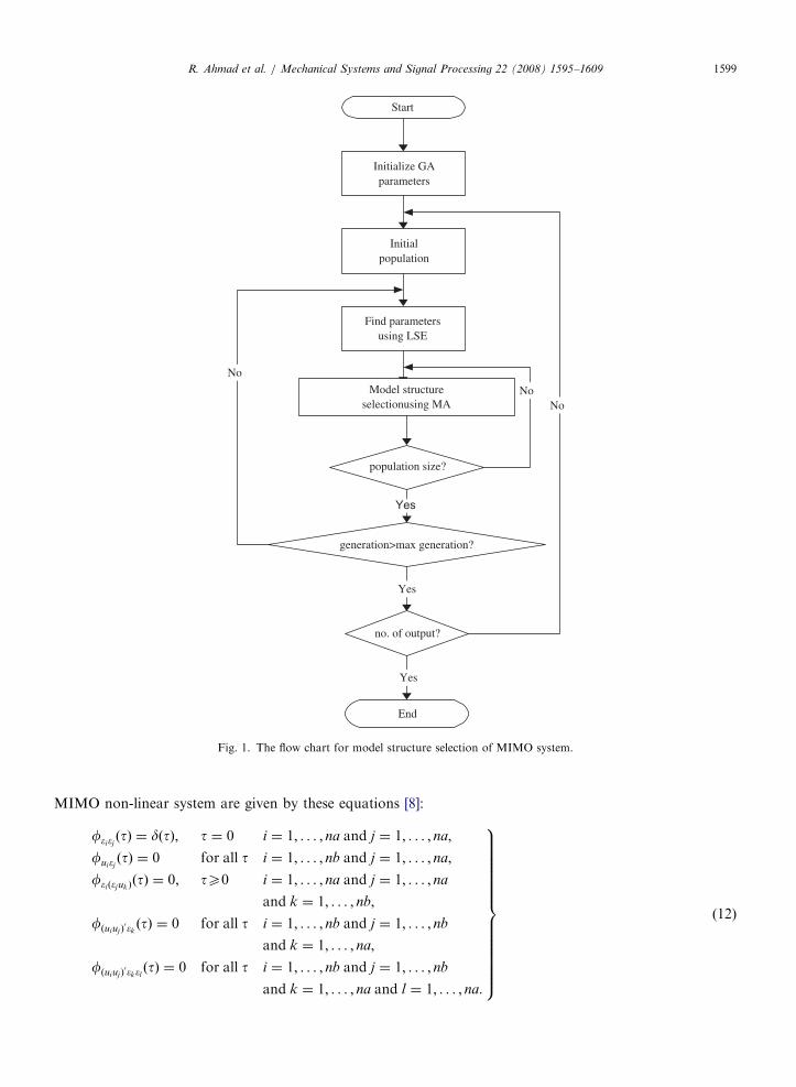
Model structure selection using MA has been used as an alternative to determine the model structure of thesystem. The procedure of the algorithm is shown as a flowchart in Fig. 1. The algorithm attempts to optimisethe model structure of multivariable systems and the procedure remains the same as for SISO system asexplained in [28] with some additional steps for the MIMO procedure.
3.3. Model validity tests
Model validation is the final procedure in system identification. The objective is to check whether the modelfits the data adequately without any bias. Expanding the one-step-ahead prediction (OSA) of SISO systemsinto its MIMO form gives
yOSAiðtÞ ¼ F i½ðyiðt� 1Þ; . . . ; yiðt� nyÞ; ujðt� 1Þ; . . . ; ujðt� nuÞÞ�, (10)
where i ¼ 1,y, na and j ¼ 1,y, nb. Similarly, the model predicted output (MPO) is defined as
yMPOiðtÞ ¼ F ½ðyMPOi
ðt� 1Þ; . . . ; yMPOiðt� nyÞ; ujðt� 1Þ; . . . ; ujðt� nuÞ�, (11)
where the model output is based on the past predicted output and input data. Unlike OSA which usesobserved data at time t to predict output at time t+1, MPO is an efficient model assessment because theprediction errors at previous time instants are inherited by the predictions at later time instant making it moresensitive to the unmodelled terms and incorrect model structure [29,31]. The correlation tests to validate
ARTICLE IN PRESS
Start
Initialize GAparameters
Initialpopulation
Find parametersusing LSE
Model structureselectionusing MA
population size?
No
Yes
generation>max generation?
Yes
no. of output?
No
No
Yes
End
Fig. 1. The flow chart for model structure selection of MIMO system.
R. Ahmad et al. / Mechanical Systems and Signal Processing 22 (2008) 1595–1609 1599
MIMO non-linear system are given by these equations [8]:
f�i�jðtÞ ¼ dðtÞ; t ¼ 0 i ¼ 1; . . . ; na and j ¼ 1; . . . ; na;
fui�jðtÞ ¼ 0 for all t i ¼ 1; . . . ; nb and j ¼ 1; . . . ; na;
f�ið�jukÞðtÞ ¼ 0; tX0 i ¼ 1; . . . ; na and j ¼ 1; . . . ; na
and k ¼ 1; . . . ; nb;
fðuiujÞ0�kðtÞ ¼ 0 for all t i ¼ 1; . . . ; nb and j ¼ 1; . . . ; nb
and k ¼ 1; . . . ; na;
fðuiujÞ0�k�l ðtÞ ¼ 0 for all t i ¼ 1; . . . ; nb and j ¼ 1; . . . ; nb
and k ¼ 1; . . . ; na and l ¼ 1; . . . ; na:
9>>>>>>>>>>>>>>=>>>>>>>>>>>>>>;
(12)
ARTICLE IN PRESSR. Ahmad et al. / Mechanical Systems and Signal Processing 22 (2008) 1595–16091600
Another performance measure is called Error Index (EI) given by
Error Index ¼
ffiffiffiffiffiffiffiffiffiffiffiffiffiffiffiffiffiffiffiffiffiffiffiffiffiffiffiffiffiffiffiPðyðtÞ � yðtÞÞ2P
y2ðtÞ
s, (13)
where the performance of the model is also evaluated using normalised root mean square of the residual. Thevalue ranges between 0 and 1 and it gives the measure of relative closeness between the predicted output andthe measured output.
3.4. Validation of the algorithm
The effectiveness of the proposed algorithm is investigated for various simulated MIMO systems beforeimplementing it to an experimental data. Two discrete-time multivariable non-linear systems were simulatedto produce input–output data to be used for structure selection using the algorithm as follows:
System 1 : y1ðtÞ ¼ 0:5y1ðt� 1Þ þ uðt� 2Þ þ 0:1y2ðt� 1Þuðt� 1Þ þ eðtÞ;
y2ðtÞ ¼ 0:9y1ðt� 1Þ þ uðt� 1Þ þ 0:2y2ðt� 1Þuðt� 2Þ þ eðtÞ;
System 2 : y1ðtÞ ¼ 0:5y1ðt� 2Þ þ u1ðt� 2Þ þ 0:1y2ðt� 1Þu1ðt� 1Þ þ eðtÞ;
y2ðtÞ ¼ 0:9y2ðt� 2Þ þ u2ðt� 1Þ þ 0:2y2ðt� 1Þu2ðt� 2Þ þ eðtÞ;
where e(t) is a white noise in the range of [�0.01,0.01]. The input–output data consist of 500 measurements.These known structure models are selected to validate the ability for the algorithm to determine the correctmodel structure. Non-linear models with the values for ny, nu, and l equal to 2 were used to fit these data.System 1 is a one-input and two-output system and the maximum number of terms is 14 that give 16 383possible model structures. System 2 is a two-input two-output system and the maximum number of terms is 27with 134 217 727 possible model structures. The parameters used in the algorithms are 5, 0.6 and 0.01 forpopulation size, pc and pm, respectively.
After 30 generations, the algorithm yields the model given in Tables 1 and 2 with the values of error indexfor each output. The results show that the algorithm is able to identify the correct model structures for bothsystems. The simulation results indicate that the algorithm which was initially applied to SISO systems iscapable to identify the model structures of these multivariable systems.
A number of case studies have been conducted to study the applications of the proposed algorithm onexperimental data of real systems [30]. However, only one case study is reported here. The goal of thesimulation study is to investigate the effectiveness of the algorithm in modelling MIMO systems based on theexperimental data where their exact structures are unknown.
4. Modelling continuous stirred tank reactor (CSTR)
In a chemical process, a model can be developed based on mass and energy balance equations, reactionrates, transport rates for heat and other chemical or physical relationships [25]. This type of modelling is timeconsuming and expensive and may result with a complex model which sometimes is not easily interpretable by
Table 1
Identified structure for System 1
Output Terms Estimates Error index
1 y1(t–1) 0.4990 0.0085
u(t–2) 1.0000
y2(t–1)u(t–1) 0.1000
2 y1(t–1) 0.8994 0.0068
u(t–1) 0.9998
y2(t–1)u(t–2) 0.1993
ARTICLE IN PRESS
Table 2
Identified structure for System 2
Output Terms Estimates Error index
1 y1(t–1) 0.4993 0.0088
u1(t–2) 0.9995
y2(t–1)u1(t–1) 0.1000
2 y2(t–2) 0.8999 0.0039
u2(t–1) 0.9999
y2(t–1)u2(t–2) 0.1997
R. Ahmad et al. / Mechanical Systems and Signal Processing 22 (2008) 1595–1609 1601
designers to establish a control policy. An alternative modelling technique is to look initially at the system intotal, record the response of the process after applying a known input and use the collected data fordetermination of data-based description of the system or based on system identification procedure. Theformulated mathematical description of the system can therefore provide basis for analysis, design andprediction while the essential causal of input and output relationship can still be captured [2]. Furthermore,model development and simulation time is much reduced compared with developing theoretical or physicalmodels.
One of the most important unit operations in a chemical process is a chemical reactor, which is a non-linearsystem and where the chemical reaction in the reactor is either exothermic or endothermic. An example of achemical reactor is a perfectly mixed, jacketed continuously stirred tank reactor or CSTR. The CSTR processis a multivariable system, with MIMO control configuration [7]. In this study, a perfectly mixed, continuouslystirred tank reactor with exothermic reactions is considered and is referred as System 3. The theoretical detailsof this process can be found in [32].
System identification is a technique of modelling the relation between the input and output data without theknowledge of the above equations and it is much less expensive to develop. The ability to develop reliabledescriptive models using input–output model at low cost is very useful in process monitoring and prediction.In this section, a non-linear identification technique is employed based on MA as described before to modelthe relation between the coolant jacket temperature and the reaction temperature and reaction concentration.
4.1. Jacketed continuous stirred tank reactor
In a jacketed CSTR, a fluid stream is continuously fed to the reactor and another fluid stream iscontinuously removed from the reactor. A cooling jacket surrounding the reactor removes the heat generatedby the reaction. In this case study, the input and output data from a pilot scale chemical reactor designed byHussain et al. [33] have been used for the identification purposes. As the reactor is perfectly mixed, theconcentration and temperature at the exit stream are the same as the reactor fluid. The heat of the reactiongenerated by the process is simulated by a controlled and regulated saturated steam flow rate through a steamcoil emerged in the reactor. A jacket surrounding the reactor also has feed and exit streams assumed to beperfectly mixed. Energy produced in the reactor process passes through the walls into the jacket and it removesany heat generated in the tank.
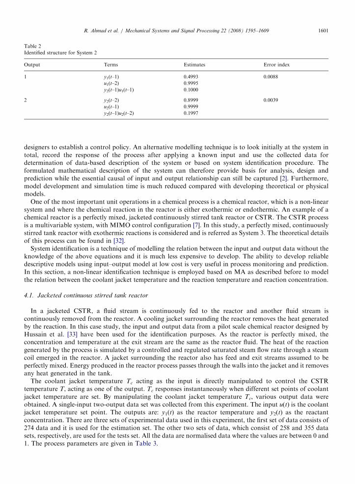
The coolant jacket temperature Tc acting as the input is directly manipulated to control the CSTRtemperature T, acting as one of the output. Tc responses instantaneously when different set points of coolantjacket temperature are set. By manipulating the coolant jacket temperature Tc, various output data wereobtained. A single-input two-output data set was collected from this experiment. The input u(t) is the coolantjacket temperature set point. The outputs are: y1(t) as the reactor temperature and y2(t) as the reactantconcentration. There are three sets of experimental data used in this experiment, the first set of data consists of274 data and it is used for the estimation set. The other two sets of data, which consist of 258 and 355 datasets, respectively, are used for the tests set. All the data are normalised data where the values are between 0 and1. The process parameters are given in Table 3.
ARTICLE IN PRESSR. Ahmad et al. / Mechanical Systems and Signal Processing 22 (2008) 1595–16091602
4.2. Process model
Most chemical processes are non-linear, and non-linear mathematical models can adequately describe theirbehaviour by either using principle of material and energy balance or based on process input and outputinformation. For the jacketed CSTR, the models are developed using the material and energy balance insidethe reactor where the process can be described by an ordinary differential equation (ODE). The advantages ofmodelling using the physical models are the ability to describe the internal dynamics of the process and toinclude mathematical description of the process. However, there are some disadvantages associated with thistype of modelling such as the high cost of model development as well as the limitations of including details ofthe process due to the lack of information about various model parameters.
Table 3
Process parameters for jacketed CSTR [25]
F 0.16m3/h
V 0.16m3
K0 4,878,000 h�1
(�DH) 20,923kcal/mole
UA 185kcal/hK
Caf 25 kgmol/m3
Tf 303K
rCp 1000kcal/(m3K)
R 1.987 cal/molK
E/R 5.96� 103K
Tc 318.15K
Ca 24.51 kgmol/m3
T 310K
Table 4
Identified model for System 3 using MA
Output Terms Estimates Error index
1 y1(t–1) 2.607 0.0496
y2(t–1) 3.259
y1(t–1)y2(t–1) �1.400
y1(t–1)y2(t–2) �3.255
y1(t–1)u(t–1) 0.367
y1(t–1)u(t–2) �0.214
y12(t–2) �1.786
y1(t–2)u(t–2) 0.153
y22(t–1) �3.253
y2(t–1)u(t–1) �1.111
y2(t–1)u(t–2) 0.685
y2(t–2)u(t–1) 1.282
y2(t–2)u(t–2) �0.704
u2(t–1) �0.147
2 y1(t–1) 1.145 0.0464
y12(t–1) �0.937
y1(t–1)u(t–1) �0.185
y1(t–1)u(t–2) �0.182
y22(t–1) 0.993
y2(t–1)u(t–1) �0.100
y2(t–2)u(t–2) �0.094
u2(t–2) 0.168
ARTICLE IN PRESSR. Ahmad et al. / Mechanical Systems and Signal Processing 22 (2008) 1595–1609 1603
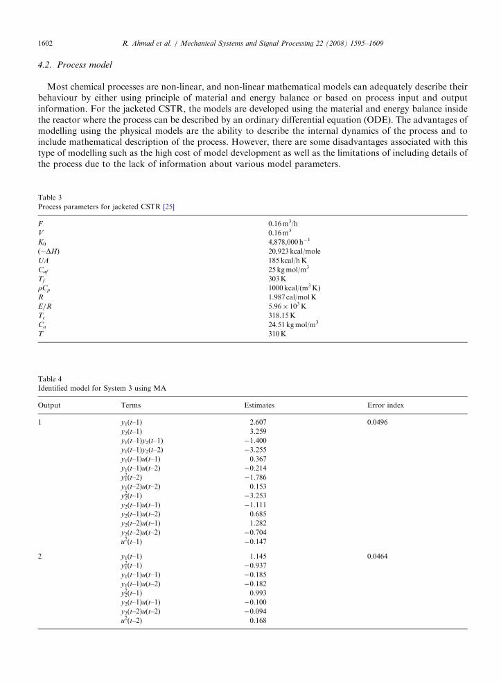
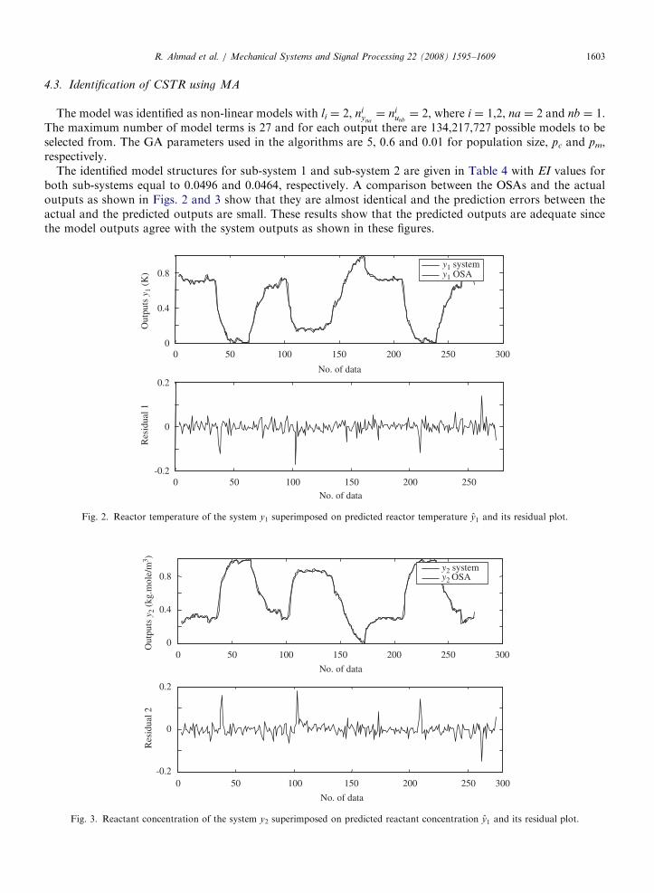
4.3. Identification of CSTR using MA
The model was identified as non-linear models with li ¼ 2, niyna¼ ni
unb¼ 2, where i ¼ 1,2, na ¼ 2 and nb ¼ 1.
The maximum number of model terms is 27 and for each output there are 134,217,727 possible models to beselected from. The GA parameters used in the algorithms are 5, 0.6 and 0.01 for population size, pc and pm,respectively.
The identified model structures for sub-system 1 and sub-system 2 are given in Table 4 with EI values forboth sub-systems equal to 0.0496 and 0.0464, respectively. A comparison between the OSAs and the actualoutputs as shown in Figs. 2 and 3 show that they are almost identical and the prediction errors between theactual and the predicted outputs are small. These results show that the predicted outputs are adequate sincethe model outputs agree with the system outputs as shown in these figures.
0 50 100 150 200 250 3000
0.4
0.8
No. of data
Out
puts
y1
(K)
y1 system y1 OSA
0 50 100 150 200 250-0.2
0
0.2
No. of data
Res
idua
l 1
Fig. 2. Reactor temperature of the system y1 superimposed on predicted reactor temperature y1 and its residual plot.
0 50 100 150 200 250 3000
0.4
0.8
Out
puts
y2
(kg.
mol
e/m
3 )
y2 system y2 OSA
0 50 100 150 200 250-0.2
0
0.2
Res
idua
l 2
300
No. of data
No. of data
Fig. 3. Reactant concentration of the system y2 superimposed on predicted reactant concentration y1 and its residual plot.
ARTICLE IN PRESSR. Ahmad et al. / Mechanical Systems and Signal Processing 22 (2008) 1595–16091604
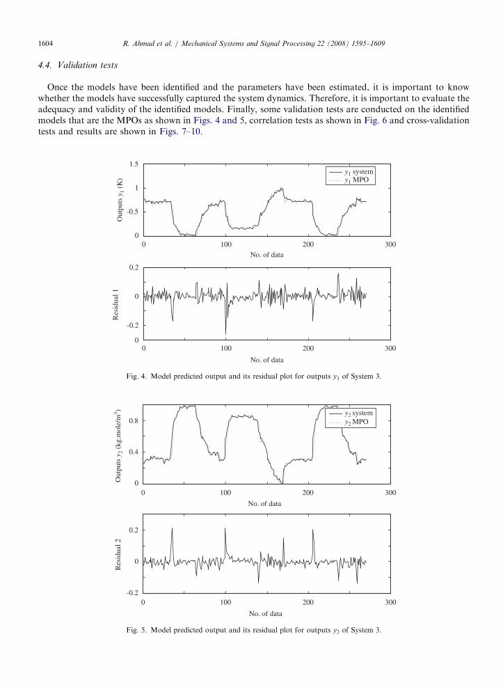
4.4. Validation tests
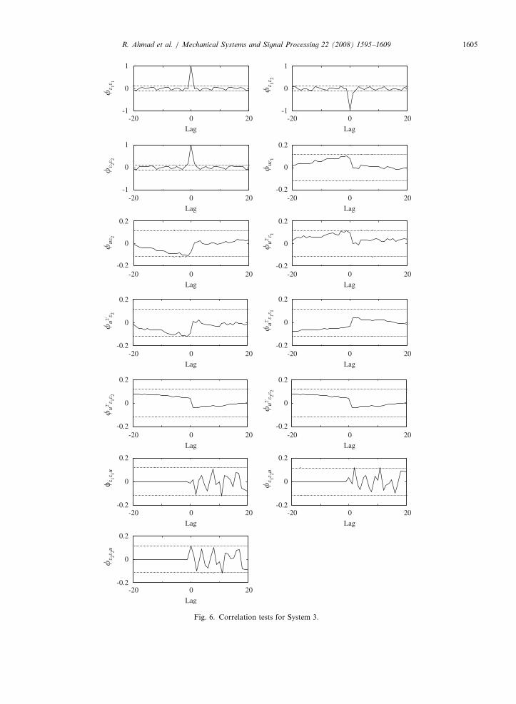
Once the models have been identified and the parameters have been estimated, it is important to knowwhether the models have successfully captured the system dynamics. Therefore, it is important to evaluate theadequacy and validity of the identified models. Finally, some validation tests are conducted on the identifiedmodels that are the MPOs as shown in Figs. 4 and 5, correlation tests as shown in Fig. 6 and cross-validationtests and results are shown in Figs. 7–10.
0 3000
-0.5
1
1.5y1 system y1 MPO
0 300
-0.2
0
0.2
100 200
100 2000
Out
puts
y1
(K)
Res
idua
l 1
No. of data
No. of data
Fig. 4. Model predicted output and its residual plot for outputs y1 of System 3.
0 3000
0.4
0.8y2 system y2 MPO
0 300-0.2
0
0.2
Res
idua
l 2
100
100
Out
puts
y2
(kg.
mol
e/m
3 )
No. of data
No. of data
200
200
Fig. 5. Model predicted output and its residual plot for outputs y2 of System 3.
ARTICLE IN PRESS
-20 0 20-1
0
1
Lag
-20 0 20
Lag
-20 0 20
Lag
-20 0 20
Lag
-20 0 20
Lag
-20 0 20
Lag
-20 0 20
Lag
-20 0 20
Lag
-20 0 20
Lag
-20 0 20
Lag
-20 0 20
Lag
-20 0 20
Lag
-20 0 20
Lag
-1
0
1
-1
0
1
-0.2
0
0.2
-0.2
0
0.2
-0.2
0
0.2
-0.2
0
0.2
-0.2
0
0.2
-0.2
0
0.2
-0.2
0
0.2
-0.2
0
0.2
-0.2
0
0.2
-0.2
0
0.2
�� 1�
1�
� 2�2
�u�
2�
u2'� 2
�u2'
� 1�2
φ �1�
1u�
� 2�2u
�� 1�
2u�
u2'� 2�
2�
u2'� 1�
1�
u2'� 1
�u�
1�
� 1�2
Fig. 6. Correlation tests for System 3.
R. Ahmad et al. / Mechanical Systems and Signal Processing 22 (2008) 1595–1609 1605

ARTICLE IN PRESS
0 100 200 3000
0.4
0.8 y1 system y1 predicted
0 100 200 300-0.1
0
0.1
Out
puts
y1
(K)
Res
idua
l 1
No. of data
No. of data
Fig. 7. Cross-validation results of output 1 from data 2.
0 100 200 300 0
0.4
0.8 y1 system y1 predicted
0 100 200 300 -0.1
0
0.1
No. of data
Res
idua
l 2
Out
puts
y2
(kg.
mol
e/m
3 )
Fig. 8. Cross-validation results of output 2 from data 2.
R. Ahmad et al. / Mechanical Systems and Signal Processing 22 (2008) 1595–16091606
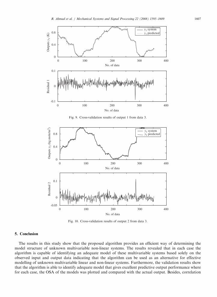
The MPO tests as shown in Figs. 4 and 5, respectively, are good because the MPOs follow the systemoutputs very well. The values for error index for the models are 0.0770 and 0.0583 for outputs 1 and 2,respectively, which are relatively small. The correlation tests as shown Fig. 6 confirm that the models areadequate because the dash lines for the upper and lower bounds that indicate a deviation of 5% show that thetests lie within the 95% confidence band. To further validate the models, two different sets of collected dataare used for tests sets or cross-validation tests and the results are illustrated in Figs. 7–10. In order to give aquantitative measurement, the values of EI for those models are calculated. The values are 0.0449 for modeloutput 1, 0.0435 for model output 2 using the second data set. The values of error index are 0.0428 for modeloutput 1 and 0.0277 for model output 2 using the third data set. These validation results also confirm that thealgorithm provide good approximations for modelling the jacketed CSTR.
ARTICLE IN PRESS
0 100 200 300 400 0
0.4
0.8 y1 system y1 predicted
0 100 200 300 400 -0.1
0
0.1
Res
idua
l 1O
utpu
ts y
1 (K
)
No. of data
No. of data
Fig. 9. Cross-validation results of output 1 from data 3.
0 100 200 300 4000
0.4
0.8 y1 system y1 predicted
0 100 200 300 400 -0.05
0
0.1
Res
idua
l 2
No. of data
Out
puts
y2
(kg.
mol
e/m
3 )
No. of data
Fig. 10. Cross-validation results of output 2 from data 3.
R. Ahmad et al. / Mechanical Systems and Signal Processing 22 (2008) 1595–1609 1607
5. Conclusion
The results in this study show that the proposed algorithm provides an efficient way of determining themodel structure of unknown multivariable non-linear systems. The results revealed that in each case thealgorithm is capable of identifying an adequate model of these multivariable systems based solely on theobserved input and output data indicating that the algorithm can be used as an alternative for effectivemodelling of unknown multivariable linear and non-linear systems. Furthermore, the validation results showthat the algorithm is able to identify adequate model that gives excellent predictive output performance wherefor each case, the OSA of the models was plotted and compared with the actual output. Besides, correlation

ARTICLE IN PRESSR. Ahmad et al. / Mechanical Systems and Signal Processing 22 (2008) 1595–16091608
tests results for the turbo-alternator and the jacketed CSTR reveal that the fitted models are almost unbiasedand have correctly captured the system dynamic. The results presented show that the algorithm can be used asan alternative for predicting the dynamic behaviour of some systems or processes.
Acknowledgement
The authors would like to acknowledge the supports from Universiti Teknologi Malaysia under Vote No.71752 throughout this research.
References
[1] R. Johansson, System Modeling and Identification, Prentice-Hall, Englewood Cliffs, NJ, 1993.
[2] L. Ljung, System Identification Theory for the User, Prentice-Hall, Englewood Cliffs, NJ, 1999.
[3] T. Soderstrom, P. Stoica, System Identification, Prentice-Hall, Hertfordshire, 1989.
[4] J.K. McElveen, K.R. Lee, J.E. Bennet, Identification of multivariable linear systems from input/output measurements, IEEE
Transactions on Industrial Electronics 39 (3) (1992) 189–193.
[5] P. Stoica, M. Jansson, A transfer function approach to MIMO system identification, in: Proceeding of the 36th Conference on
Decision and Control, Arizona, 1992, pp. 2400–2405.
[6] S. Munzir, H.M. Mohamed, M.Z. Abdulmuin, A new approach for modeling and control of MIMO nonlinear systems, in:
Proceedings of the TENCON, Kuala Lumpur, 2000, pp. 489–497.
[7] A.H. Kemna, W.E. Larimore, D.E. Seborg, D.A. Mellichamp, On-line multivariable identification and control of chemical processes
using canonical variate analysis, in: Proceeding of the American Control Conference, Maryland, 1994, pp. 1650–1654.
[8] S.A. Billings, S. Chen, M.J. Korenberg, Identification of MIMO non-linear systems using forward-regression orthogonal estimator,
International Journal of Control 50 (6) (1989) 2157–2189.
[9] N. Chaiyaratana, A.M.S. Zalzala, Recent developments in evolutionary and genetic algorithms: theory and application, in:
Proceedings of the Conference on Genetic Algorithms in Engineering Systems: Innovation and Applications, vol. 446, 1997,
pp. 270–277.
[10] O.E. Canyurt, Estimation of welded joint strength using genetic algorithm, International Journal of Mechanical Sciences 47 (2005)
1249–1261.
[11] D.J. Fonseca, S. Shishoo, T.C. Lim, D.S. Chen, A genetic algorithm approach to minimize transmission error of automative spur gear
sets, Applied Artificial Intelligence 19 (2) (2005) 153–179.
[12] M. Gestal, M.P. Gomez-Carracedo, J.M. Andrade, J. Dorado, E. Fernandez, D. Prada, A. Pazos, Selection of variables by genetic
algorithms to classify apple beverages by artificial neural networks, Applied Artificial Intelligence 19 (2) (2005) 181–198.
[13] T. Minerva, I. Poli, Building ARMA models with genetic algorithms, in: E.J.W. Boers, et al. (Eds.), Lecture Notes in Computer
Science, Springer, Berlin, Heidelberg, 2001.
[14] R. Ahmad, H. Jamaluddin, M.A. Hussain, Model structure selection for a discrete-time non-linear system using genetic algorithm,
Proceedings of the Institution of Mechanical Engineers Part I—Journal of Systems and Control Engineering 218 (12) (2004) 85–98.
[15] Q. Chen, K. Worden, P. Peng, A.Y.T. Leung, Genetic algorithm with an improved fitness function for (N)ARX modeling,
Mechanical Systems and Signal Processing 21 (2007) 994–1007.
[16] J.M. Nougues, M.D. Grau, L. Puigjaner, Parameter estimation with genetic algorithm in control of fed-batch reactors, Chemical
Engineering and Processing 41 (2002) 303–309.
[17] W.-D. Chang, An improved real-coded genetic algorithm for parameters estimation of nonlinear systems, Mechanical Systems and
Signal Processing 20 (2006) 236–246.
[18] G.C. Luh, C.Y. Wu, Inversion control nonlinear system with an inverse NARX model identified using genetic algorithms,
Proceedings of the Institution of Mechanical Engineers Part 1-Journal of Systems and Control in Engineering 214 (1999) 259–271.
[19] Y. Liu, L. Ma, J. Zhang, GA/SA/TS hybrid algorithms for reactive power optimization, Power Engineering Society Summer Meeting,
Seattle, WA, IEEE Press, New York, 2000, pp. 245–249.
[20] D. Whitley, V. Gordon, K. Mathias, K. Lamarkian, Evolution, the Baldwin effect and function optimization, in: Y. Davidor, H.P.
Schwefel, R. Manner (Eds.), Parallel Problem Solving from Nature-PPSN III 866, Springer, Berlin, 1994, pp. 6–15.
[21] P. Moscato, On evolution, search, optimization, genetic algorithms and martial arts: towards memetic algorithm, Technical Report,
826, California Institute of Technology, Pasadena, CA, USA, 1989.
[22] P.M. Franca, A. Mendes, P. Moscato, A memetic algorithm for the total tardiness single machine scheduling problem, European
Journal of Operational Research 132 (2001) 224–242.
[23] N. Krasnogor, J. Smith, A memetic algorithm with self-adaptive loal search: TSP as a case study, in: D. Whitley, D. Golberg, E.
Cantu-Paz, L. Spector (Eds.), Proceedings of the GECCO-2000, Las Vegas, NV, Morgan-Kaufman, Los Altos, CA, pp. 987–994.
[24] P. Merz, B. Freisleben, A comparison of memetic algorithms, tabu search, and ant colonies for the quadratic assignment problem, in:
Proceedings of the Congress on Evolutionary Computation, IEEE Service Center, 1999, pp. 2063–2070.
[25] W.L. Luyben, Process Modeling, Simulation, and Control for Chemical Engineers, International ed., McGraw-Hill, Singapore, 1990.

ARTICLE IN PRESSR. Ahmad et al. / Mechanical Systems and Signal Processing 22 (2008) 1595–1609 1609
[26] I.J. Leontaritis, S.A. Billings, Input–output parametric models for non-linear systems, Part I: deterministic non-linear systems,
International Journal of Control 41 (2) (1985) 303–328.
[27] S. Chen, S.A. Billings, Representations of nonlinear systems: the NARMAX model, International Journal of Control 49 (3) (1989)
1013–1032.
[28] R. Ahmad, H. Jamaluddin, M.A. Hussain, Selection of a model structure in system identification using memetic algorithm, in:
Proceedings of the Second International Conference on Artificial Intelligence in Engineering and Technology, vol. 2, 2004,
pp. 714–720.
[29] Z. Michalewicz, Genetic Algorithms+Data Structure ¼ Evolution Programs, third ed, Springer, Berlin, 1999.
[30] R. Ahmad, Identification of discrete-time dynamic systems using modified genetic algorithm, Ph.D. Thesis, Universiti Teknologi
Malaysia, 2004.
[31] S.A. Billings, K.Z. Mao, Model identification and assessment based on model predicted output, Research Report No. 714,
Department of Automatic Control and Systems Engineering, University of Sheffield, UK, 1998.
[32] B.W. Bequette, Process Dynamics—Modeling, Analysis and Simulation, Module 9, Prentice-Hall, Englewood Cliffs, NJ, 1998, p. 562.
[33] M.H. Hussain, M.S. Malik, M.Z. Sulaiman, A.K. Abdul Wahab, Design and control of experimental partially simulated exothermic
reactor system, in: Regional Symposium of Chemical Engineering, Proceeding, 22–24 November, Songkhla, Thailand, 1999, pp. B26-
1–B26-4.


![A Memetic Algorithm for Reconstructing Cross-Cut Shredded … · 2010-11-16 · A Memetic Algorithm for RCCSTD 3 reconstruction of cross-cut shredded (text) documents (RCCSTD) [15,16,20]](https://img.pdfslide.us/doc/110x75/5e7fb8937c970f37a8303d95/a-memetic-algorithm-for-reconstructing-cross-cut-shredded-2010-11-16-a-memetic.jpg)