Application of Liquid Chromatography-Tandem Mass

University of Tennessee, Knoxville University of Tennessee, Knoxville

TRACE: Tennessee Research and Creative TRACE: Tennessee Research and Creative

Exchange Exchange

Masters Theses Graduate School

12-2011

Application of Liquid Chromatography-Tandem Mass Application of Liquid Chromatography-Tandem Mass

Spectrometry Techniques to the Study of Two Biological Systems Spectrometry Techniques to the Study of Two Biological Systems

Mary E. Eisenhauer [email protected]

Follow this and additional works at: https://trace.tennessee.edu/utk_gradthes

Recommended Citation Recommended Citation Eisenhauer, Mary E., "Application of Liquid Chromatography-Tandem Mass Spectrometry Techniques to the Study of Two Biological Systems. " Master's Thesis, University of Tennessee, 2011. https://trace.tennessee.edu/utk_gradthes/1066

This Thesis is brought to you for free and open access by the Graduate School at TRACE: Tennessee Research and Creative Exchange. It has been accepted for inclusion in Masters Theses by an authorized administrator of TRACE: Tennessee Research and Creative Exchange. For more information, please contact [email protected].

https://trace.tennessee.edu/

https://trace.tennessee.edu/

https://trace.tennessee.edu/utk_gradthes

https://trace.tennessee.edu/utk-grad

https://trace.tennessee.edu/utk_gradthes?utm_source=trace.tennessee.edu%2Futk_gradthes%2F1066&utm_medium=PDF&utm_campaign=PDFCoverPages

mailto:[email protected]

To the Graduate Council:

I am submitting herewith a thesis written by Mary E. Eisenhauer entitled "Application of Liquid

Chromatography-Tandem Mass Spectrometry Techniques to the Study of Two Biological

Systems." I have examined the final electronic copy of this thesis for form and content and

recommend that it be accepted in partial fulfillment of the requirements for the degree of

Master of Science, with a major in Chemistry.

Shawn R. Campagna, Major Professor

We have read this thesis and recommend its acceptance:

Michael Best, Michael Sepaniak

Accepted for the Council:

Carolyn R. Hodges

Vice Provost and Dean of the Graduate School

(Original signatures are on file with official student records.)

Application of Liquid Chromatography-Tandem Mass Spectrometry

Techniques to the Study of Two Biological Systems

A Thesis Presented for the

Master of Science

Degree

The University of Tennessee, Knoxville

Mary E. Eisenhauer

December 2011

ii

Dedication

For JP, LP, and Olive

iii

Acknowledgements

I would like to first thank my family, for their continuous love, support, patience, and

understanding throughout my life and scholastic career. Thank you to my committee members

Dr. Best and Dr. Sepaniak, for their support and time spent. I would also like to acknowledge my

unofficial committee member and collaborator Dr. Jason Collier, as well as the Collier lab for

their hard work. Next, I must thank Dr. Campagna, for helping me realize my potential, but for

also helping me reach my career goals as an educator. Thank you to my wonderful group

members, Sneha Belapure, Jessica Gooding, Amanda May and Jesse Middleton, for their

support and friendship. I could not have asked for a better group of people to work with. A

special acknowledgement is owed to Jess and Amanda for teaching me everything I know, but

more importantly, for their friendship over the past two years. I would not have made it without

them, and I truly appreciate everything they have done for me.

iv

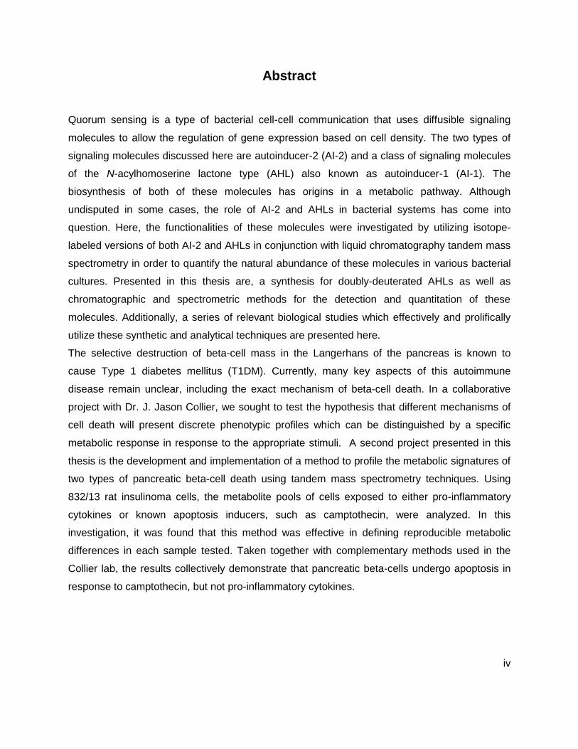
Abstract

Quorum sensing is a type of bacterial cell-cell communication that uses diffusible signaling

molecules to allow the regulation of gene expression based on cell density. The two types of

signaling molecules discussed here are autoinducer-2 (AI-2) and a class of signaling molecules

of the N-acylhomoserine lactone type (AHL) also known as autoinducer-1 (AI-1). The

biosynthesis of both of these molecules has origins in a metabolic pathway. Although

undisputed in some cases, the role of AI-2 and AHLs in bacterial systems has come into

question. Here, the functionalities of these molecules were investigated by utilizing isotope-

labeled versions of both AI-2 and AHLs in conjunction with liquid chromatography tandem mass

spectrometry in order to quantify the natural abundance of these molecules in various bacterial

cultures. Presented in this thesis are, a synthesis for doubly-deuterated AHLs as well as

chromatographic and spectrometric methods for the detection and quantitation of these

molecules. Additionally, a series of relevant biological studies which effectively and prolifically

utilize these synthetic and analytical techniques are presented here.

The selective destruction of beta-cell mass in the Langerhans of the pancreas is known to

cause Type 1 diabetes mellitus (T1DM). Currently, many key aspects of this autoimmune

disease remain unclear, including the exact mechanism of beta-cell death. In a collaborative

project with Dr. J. Jason Collier, we sought to test the hypothesis that different mechanisms of

cell death will present discrete phenotypic profiles which can be distinguished by a specific

metabolic response in response to the appropriate stimuli. A second project presented in this

thesis is the development and implementation of a method to profile the metabolic signatures of

two types of pancreatic beta-cell death using tandem mass spectrometry techniques. Using

832/13 rat insulinoma cells, the metabolite pools of cells exposed to either pro-inflammatory

cytokines or known apoptosis inducers, such as camptothecin, were analyzed. In this

investigation, it was found that this method was effective in defining reproducible metabolic

differences in each sample tested. Taken together with complementary methods used in the

Collier lab, the results collectively demonstrate that pancreatic beta-cells undergo apoptosis in

response to camptothecin, but not pro-inflammatory cytokines.

v

Table of Contents

Introduction ............................................................................................................................ 1 Chapter I Achieving a Quantitative Understanding of Quorum Sensing ................................................. 2 Abstract .................................................................................................................................. 3 Background and Significance ................................................................................................. 4

Quorum Sensing ................................................................................................................ 5 AI-2 Mediated Quorum Sensing ......................................................................................... 6 N-Acylhomoserine Lactone Mediated Quorum Sensing ..................................................... 7 Biosynthesis of Quorum Sensing Molecules ....................................................................... 8 Vibrio harveyi and Escherichia coli Background ................................................................. 9 Analytical Methods ............................................................................................................11 High Performance Liquid Chromatography Tandem Mass Spectrometry ..........................12 Isotope Dilution Tandem Mass Spectrometry ....................................................................14

Results and Discussion .........................................................................................................14 Design Rationale for the Synthesis of Stable Isotope Labeled AHLs .................................15 Synthesis of Deuterated N-Acyl Homoserine Lactones .....................................................15 Separation and Detection of AHLs and AI-2 ......................................................................18 Profiling Bacterial Species for Autoinducer Production ......................................................20 Results: Vibrio fischeri .......................................................................................................21 Results: Edwardsiella tarda ...............................................................................................23 Characterization of an Enteropathogen .............................................................................24 Results: Yersinia enterocolitica ..........................................................................................24

Methods and Materials ..........................................................................................................30 General Methods ...............................................................................................................30 Bacterial Growth Conditions ..............................................................................................30 Chromatographic Details ...................................................................................................30 General Mass Spectrometric Detection Parameters for AI-2 and AHLs .............................31 Measurement of AI-2 Concentration [AI-2] ........................................................................31 Measurement of AHL Concentration(s) [AHL(s)] ...............................................................32 Data Handling for the Calculation of [DPD] ........................................................................32 Data Handling for the Calculation of [AHL(s)] ....................................................................33 Measurement of Glucose Concentration by Colorimetric Glucose Oxidation Assay ...........34 N-Boc-(4,4-2H2)homoserine-α-OtBu ester, 2 ......................................................................34 N-Boc-(4,4-2H2)homoserine-γ-OMs-α-OtBu ester, 3 ..........................................................35 N-Boc-(4,4-2H2)methionine-OtBu ester, 4 ..........................................................................36 (4,4-2H2)methionine, 5 .......................................................................................................36 N-Fmoc-(4,4-2H2)methionine, 6 .........................................................................................37 Representative N-Fmoc-(4,4-2H2)methionine resin loading protocol ..................................37 Representative Synthesis of (2H2) AHLs, N-octanoyl-(4,4-2H2) acylhomoserine lactone ....38

Chapter II Determining Metabolic Profiles of Rat Insulinoma Cells.........................................................41 Abstract .................................................................................................................................42 Background and Significance ................................................................................................43

Metabolomics Background ................................................................................................43 Metabolic Profiling vs. Metabolic Fingerprinting .................................................................44 Sample Type .....................................................................................................................44 Sampling and Extracting....................................................................................................45

vi

Analytical Methods ............................................................................................................46 Mass Spectrometry Based Metabolomics ..........................................................................46 Data Analysis ....................................................................................................................47 Pancreatic β-cell Death .....................................................................................................47 Pancreatic β-cell Death is likely the Result of a Non-Apoptotic Mechanism .......................48

Results and Discussion .........................................................................................................50 Distinction between Cell Death .........................................................................................50 Metabolic Profiling by Tandem Mass Spectrometry ...........................................................51

Methods and Materials ..........................................................................................................53 General Methods ...............................................................................................................53 Cell Extraction Procedure ..................................................................................................53 Chromatographic Details ...................................................................................................53 Mass Spectrometric Detection Parameters........................................................................54 Data Handling and Statistical Anaylsis ..............................................................................55

Conclusion ............................................................................................................................56 References ............................................................................................................................57 Appendix ...............................................................................................................................65

NMR Spectra.......................................................................................................................66 Tabulated Data....................................................................................................................79 Metabolites Measured.......................................................................................................106

Vita...................................................................................................................................... 110

vii

List of Tables

Table 1: Structure, Abbreviations and SRMs for AHLs ..............................................................18 Table 2: Strains Profiled ............................................................................................................20 Table 3: V. fischeri strain ES114 [AHLs] Used in Figure 6A and 7B ..........................................79 Table 4: V. fischeri strain MJ-1 [AHLs] Used in Figure 6B and 7A .............................................80 Table 5: V. fischeri strain CL21 [AHLs] Used in Figure 6C ........................................................81 Table 6: V. fischeri strain VCW2G7 [AHLs] Used in Figure 6D ..................................................82 Table 7: V. fischeri Cell Densities Used in Figure 6E ................................................................83 Table 8: V. fischeri strains MJ-1 and ES114 [DPD] Used in Figure 7 ........................................84 Table 9: E. tarda No Added Glucose and 0.14% Glucose Cell Density and [DPD] Figure 8 ......85 Table 10: Y. enterocolitica No Added Glucose Cell Density and [DPD]/OD Used in Figure 9 ....86 Table 11: Y. enterocolitica 0.08% Glucose Cell Density and [DPD]/OD Used in Figure 9 ..........87 Table 12: Y. enterocolitica 0.14% Glucose Cell Density and [DPD]/OD Used in Figure 9 ..........88 Table 13: Y. enterocolitica 0.20% Glucose Cell Density and [DPD]/OD Used in Figure 9 ..........89 Table 14: Y. enterocolitica No Added Glucose [DPD] and % Glucose Used in Figure 10A ........90 Table 15: Y. enterocolitica 0.08% Glucose [DPD] and % Glucose Used in Figure 10B .............91 Table 16: Y. enterocolitica 0.14% Glucose [DPD] and % Glucose Used in Figure 10C .............92 Table 17: Y. enterocolitica 0.20% Glucose [DPD] and % Glucose Used in Figure 10D .............93 Table 18: Y. enterocolitica No Added Glucose Cell Density and [DPD]/OD Used in Figure 11 ..94 Table 19: Y. enterocolitica 0.08% Glucose Cell Density and [DPD]/OD Used in Figure 11 ........95 Table 20: Y. enterocolitica 0.14% Glucose Cell Density and [DPD]/OD Used in Figure 11 ........96 Table 21: Y. enterocolitica 0.20% Glucose Cell Density and [DPD]/OD Used in Figure 11 ........97 Table 22: Y. enterocolitica 0.30% Glucose Cell Density and [DPD]/OD Used in Figure 11 ........98 Table 23: Y. enterocolitica 0.50% Glucose Cell Density and [DPD]/OD Used in Figure 11 ........99 Table 24: Y. enterocolitica No Added Glucose [DPD] and % Glucose Used in Figure 12A ...... 100 Table 25: Y. enterocolitica 0.08% Glucose [DPD] and % Glucose Used in Figure 12B ........... 101 Table 26: Y. enterocolitica 0.14% Glucose [DPD] and % Glucose Used in Figure 12C ........... 102 Table 27: Y. enterocolitica 0.20% Glucose [DPD] and % Glucose Used in Figure 12D ........... 103 Table 28: Y. enterocolitica 0.30% Glucose [DPD] and % Glucose Used in Figure 12E ........... 104 Table 29: Y. enterocolitica 0.50% Glucose [DPD] and % Glucose Used in Figure 12F ............ 105 Table 30: Metabolites Measured ............................................................................................. 106 Table 31: Metabolites Measured ............................................................................................. 108

viii

List of Figures and Schemes

Figure 1: Quorum sensing is cell density dependent .................................................................. 5 Scheme 1: (S)-4,5-dihydroxy-2,3-pentandione (DPD) ................................................................ 6 Scheme 2: Biosynthesis of N-acylhomoserine lactones (AHL) ................................................... 7 Figure 2: N-acylhomoserine lactones (AHLs) ............................................................................. 8 Figure 3: The Activated Methyl Cycle ......................................................................................... 9 Figure 4: Landscape depictions of AI signal/cell density ratios, and AI synthesis rates .............10 Scheme 3: Fragmentation reactions of AHLs and derivitizaion of DPD .....................................13 Scheme 4: Solution phase synthesis of (S)-[4,4,2H2]-N-Fmoc-methionine ...............................16 Scheme 5: Solid phase synthesis of various AHLs ....................................................................17 Figure 5: Chromatographic separation and detection of AHLs ..................................................19 Figure 6: Production of 3OC6, C6, C7 and C8 AHLs in V. fischeri ............................................22 Figure 7: Cascade depictions of all autoinducers produced by V. fischeri .................................23 Figure 8: Growth kinetics and DPD production in Edwardsiella tarda ........................................24 Figure 9: Average growth kinetics and [DPD]/cell # for Yersinia enterocolitica in BHI. ...............26 Figure 10: Average [DPD] and [glucose] for Yersinia enterocolitica in BHI ................................27 Figure 11: Average growth kinetics and [DPD]/cell # for Yersinia enterocolitica in LB ...............28 Figure 12: Average [DPD] and [glucose] for Yersinia enterocolitica in LB..................................29 Figure 14: Representative heatmap displaying metabolite fold changes ...................................52

1

Introduction

Life in all of its forms is fundamentally chemical in nature. At the unique intersection of chemistry

and biology, chemistry is the universal language which governs all biological systems. Over the

years, the discipline of chemical biology has grown to include the tools of the core disciplines of

chemistry such as analytical and synthetic chemistry. Applications of these tools have been

essential for the probing and understanding of relevant biological problems and questions

because many of them are in fact rooted in chemistry. The two systems, whose studies

provided the subsequent results detailed in this thesis, were investigated principally by

variations of liquid chromatography-tandem mass spectrometry techniques.

The first system presented is the primary cell-cell communication systems of bacterial species.

These systems, termed quorum sensing, are a method by which bacteria use small molecules

to send information about the status of their population density and possibly their immediate

environment. The variety of platforms used to study these systems are expansive, ranging

anywhere from genomics to classical analytical techniques. The immediate goal surrounding

research of these systems also varies. Quorum sensing pathways continue to be newly

identified in different species of bacteria and in different environments. Alternatively, the

purpose for studying quorum sensing could be to determine why these systems are present and

for what purpose they ultimately serve. The studies presented in Chapter I of this thesis will

focus on the quantitation of the small molecules involved in quorum sensing in different bacterial

species in an effort to better define the exact nature of quorum sensing systems.

The second system of interest is the global metabolism of rat insulinoma cells. These cells will

serve as a model for the human pancreatic islet cells affected by the autoimmune disease, Type

1 Diabetes mellitus (T1DM). Although the destruction of these cells is known to cause T1DM,

the exact mechanism of death is unknown. Consequently, the delineation of this mechanism is

essential for the advancement toward a cure. Most of the current studies focus on the genomic

manipulation of pathways which are known to be involved in T1DM. From a chemical

standpoint, the studies presented in Chapter II will focus on profiling the metabolism of rat

insulinoma cells in order to better understand possible mechanisms thought to be responsible

for pancreatic islet cell death.

2

Chapter 1

Achieving a Quantitative Understanding of Quorum Sensing

3

Abstract

The quorum sensing signal Autoinducer-2 (AI-2) is thought to be an interspecies signal, and

while its signaling abilities are not disputed in all cases, there has been evidence of an

alternative use for AI-2. Its biosynthesis is linked to the activated methyl cycle, which has raised

the question as to whether its function is strictly signaling, metabolic or a combination of the two.

Conversely, only gram negative bacteria are known to produce the quorum sensing signals N-

acyl homoserine lactones (AHLs) or Autoinducer 1 (AI-1). These molecules are produced by an

intersection of two biosynthesis pathways that ordinarily serve unrelated metabolic functions.

Often, one species will produce more than one AHL and/or integrate a different class of quorum

sensing molecules such as AI-2. Our lab has designed a strategy for the determination of the

role of AI-2 through detection and quantification, and previous studies employing these

strategies have led to a basic definition of quorum sensing. Currently, there are no such tools

available for the quantitation of AI-1s. From here we aimed to develop a similar set of tools for

the detection and quantitation of AHLs. First, we have designed and carried out a synthesis of

stable isotope labeled AHLs that incorporates the use of solid phase techniques, and can

produced any AHL sought-after, due to the strategic placement of the isotope into the

conserved lactone core. With these stable isotope labeled standards in hand, we then sought to

develop chromatographic and spectrometric methods in order to use the technique of isotope

dilution tandem mass spectrometry. Using all the tools developed by our lab, we were able to

accurately quantitate exact concentrations of AHLs from biological samples, as well as continue

to probe these species for AI-2 production, to begin to understand the relationship between

these different quorum sensing systems.

4

Background and Significance

For many years it had been postulated that the bacterial world possessed a means by which

cooperative behaviors could ensure that the efforts of many outweighed the efforts of few. It was

noted that the communal nature of bacteria was beneficial for survival.1 While intrinsically

interesting, the methods by which many bacteria communicate with each other are of particular

interest because of their physiological implications. One of these methods consists of the

synthesis, accumulation, and recognition of small diffusible molecules that has been termed

quorum sensing.2-4 Quorum sensing was first discovered decades ago, but it has gained interest

recently due to the role this mechanism plays in biofilm formation.5-7 Understanding the

underlying mechanisms of biofilm formation is of importance because of the role they play in

chronic infections persistent in diseases such as cystic fibrosis.8-10 Several pathogenic bacteria

have been found that produce quorum sensing-dependent biofilms, and many of them are

antibiotic resistant. The ability to interrupt these quorum sensing pathways could potentially lead

to novel anti-infective agents that have several advantages over traditional agents.11, 12

Though many significant discoveries have been made, there is still more to be understood about

quorum sensing and the molecules involved. One basic problem is the lack of a definition of the

term quorum sensing. Currently, the term is used to encompass all phenotypic expressions

which are found to be regulated by the production and recognition of diffusible chemical signals,

regardless of whether the purpose is to transmit information on local cell density. However, it is

becoming more evident with increasing interest, that the pathways and mechanisms of quorum

sensing circuits are more dynamic, diverse and complex than originally thought.13-15 For

example, there are now many reports of bacteria that posses quorum sensing machinery, yet do

not employ quorum sensing molecules in order to measure cell density. Conversely, other

bacteria utilize multiple quorum sensing molecules and systems in order to regulate a single

behavior. There are many questions about this sometimes oversimplified mechanism that need

to be answered if a definite and comprehensive understanding of quorum sensing molecules

and pathways is to be achieved.

The analytical techniques that have been used previously have been focused toward the

detection of these quorum sensing molecules in biological systems. If the original thought that

the production of these molecules is strictly a means for bacteria to essentially “count” cell

5

numbers, then quantifying these molecules should be the next logical step in determining the

information content of signaling molecules. It is our belief that characterizing the function of

quorum sensing on an individual basis will begin with the quantitation of quorum sensing

molecules. The work presented in this chapter is built upon the tools previously employed by our

lab for the quantitation of quorum sensing molecules, and demonstrates the effectiveness of

synthetic isotopically labeled internal standards coupled with unbiased and sensitive analytical

techniques for quantiation in a variety of bacterial species.

Quorum Sensing

Quorum Sensing is the term that has been given to the unique capability by which bacterial

communities monitor population and adjust behaviors accordingly, allowing them to adapt to

different environmental factors and cues. This is accomplished by a variety of small diffusible

signaling molecules, and there are now many known examples of signaling mechanisms in a

broad range of bacteria that act as quorum sensing systems. The mechanisms have been

shown to be cell density dependent; while each single cell may emit a low concentration of

these small molecules, at high cell densities high concentrations of signal will consequently be

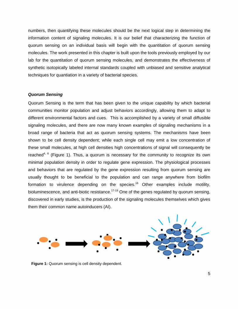
reached4, 6 (Figure 1). Thus, a quorum is necessary for the community to recognize its own

minimal population density in order to regulate gene expression. The physiological processes

and behaviors that are regulated by the gene expression resulting from quorum sensing are

usually thought to be beneficial to the population and can range anywhere from biofilm

formation to virulence depending on the species.16 Other examples include motility,

bioluminescence, and anti-biotic resistance.17-19 One of the genes regulated by quorum sensing,

discovered in early studies, is the production of the signaling molecules themselves which gives

them their common name autoinducers (AI).

Figure 1: Quorum sensing is cell density dependent.

6

Quorum sensing can be interspecies or intraspecies. Major classes of intraspecies signaling

systems include those of gram negative bacteria, which produce N-acyl homoserine lactones

(AHLs), or autoinducer 1 (AI-1s)1, and gram positive bacteria, which produce cyclic peptides

(AIPs)20. The interspecies signals that are variations of (S)-4,5-dihydroxy-2,3-pentandione

(DPD), are known as AI-2, and have been found in both gram positive and gram negative

bacteria21. Both types function similarly. The work presented in this thesis will focus on

intraspecies AI-1 molecules as well as the interspecies AI-2 signaling molecule. All AIs will be

profiled in strains that utilize one or both signaling systems. The relationship between the two

signaling pathways will be examined in species possessing both systems.

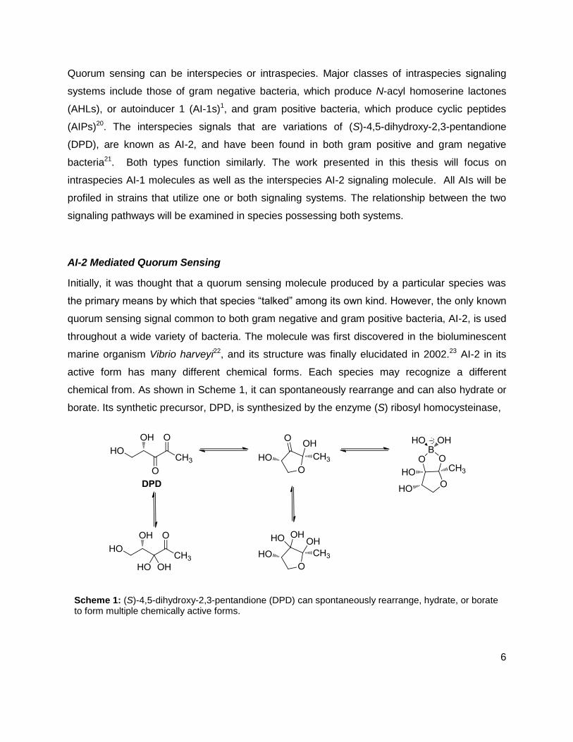
AI-2 Mediated Quorum Sensing

Initially, it was thought that a quorum sensing molecule produced by a particular species was

the primary means by which that species “talked” among its own kind. However, the only known

quorum sensing signal common to both gram negative and gram positive bacteria, AI-2, is used

throughout a wide variety of bacteria. The molecule was first discovered in the bioluminescent

marine organism Vibrio harveyi22, and its structure was finally elucidated in 2002.23 AI-2 in its

active form has many different chemical forms. Each species may recognize a different

chemical from. As shown in Scheme 1, it can spontaneously rearrange and can also hydrate or

borate. Its synthetic precursor, DPD, is synthesized by the enzyme (S) ribosyl homocysteinase,

Scheme 1: (S)-4,5-dihydroxy-2,3-pentandione (DPD) can spontaneously rearrange, hydrate, or borate to form multiple chemically active forms.

7

(LuxS).24 LuxS was identified as the AI-2 synthase in 1999, although this enzyme had previously

been described in 1968 as a part of the activated methyl cycle.25 This enzyme is well

conserved; nearly half of all sequenced bacteria, both gram positive and gram negative, contain

a LuxS homologue lending support to the idea that AI-2 is an interspecies signal.21 Throughout

this text, the terms DPD and AI-2 will be used interchangeably.

N-Acylhomoserine Lactone Mediated Quorum Sensing

Many gram negative bacteria produce one or more acylated homoserine lactone molecules to

be utilized as signaling molecules. AHL-mediated quorum sensing was first identified in V.

fischeri.26 The molecule produced was identified as (3S)-N-[3-oxo-hexyl]-homoserine lactone.

From here, several other signaling systems were identified in a wide range of species.1 Once

thought to be unique to marine bacteria, it is now clear that AHL signaling is a well conserved

regulatory system that is widespread throughout proteobacteria.27, 28 The process by which

quorum sensing bacteria produce and utilize AHLs has been extensively studied and is

relatively well characterized. Mechanistically, it is fairly simple. Acyl homoserine lactones are

synthesized by a family of proteins of the LuxI-type. When the quorum is reached, another

protein, encoded in the same lux operon, of the LuxR-type detects and interacts with

Scheme 2: A proposed mechanism for the biosynthesis of N-acylhomoserine lactones (AHL).

8

the AHLs, which then causes changes in genotypic and phenotypic expression by

transcriptional activation.29 These complexes catalyze the formation of the amide bond between

the amino group of S-adenosyl methionine (SAM) and the acyl chain from an acyl carrier protein

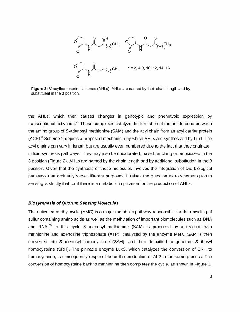
(ACP).6 Scheme 2 depicts a proposed mechanism by which AHLs are synthesized by LuxI. The

acyl chains can vary in length but are usually even numbered due to the fact that they originate

in lipid synthesis pathways. They may also be unsaturated, have branching or be oxidized in the

3 position (Figure 2). AHLs are named by the chain length and by additional substitution in the 3

position. Given that the synthesis of these molecules involves the integration of two biological

pathways that ordinarily serve different purposes, it raises the question as to whether quorum

sensing is strictly that, or if there is a metabolic implication for the production of AHLs.

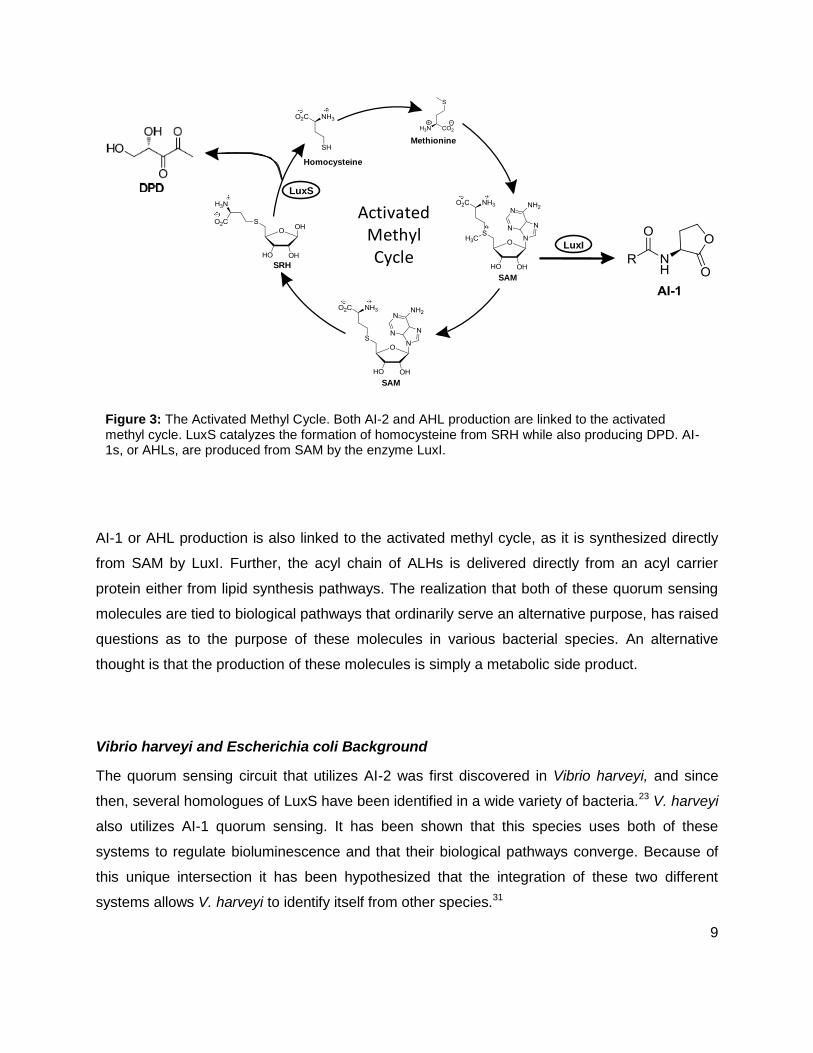
Biosynthesis of Quorum Sensing Molecules

The activated methyl cycle (AMC) is a major metabolic pathway responsible for the recycling of

sulfur containing amino acids as well as the methylation of important biomolecules such as DNA

and RNA.30 In this cycle S-adenosyl methionine (SAM) is produced by a reaction with

methionine and adenosine triphosphate (ATP), catalyzed by the enzyme MetK. SAM is then

converted into S-adenosyl homocysteine (SAH), and then detoxified to generate S-ribosyl

homocysteine (SRH). The pinnacle enzyme LuxS, which catalyzes the conversion of SRH to

homocysteine, is consequently responsible for the production of AI-2 in the same process. The

conversion of homocysteine back to methionine then completes the cycle, as shown in Figure 3.

Figure 2: N-acylhomoserine lactones (AHLs). AHLs are named by their chain length and by substituent in the 3 position.

9

AI-1 or AHL production is also linked to the activated methyl cycle, as it is synthesized directly

from SAM by LuxI. Further, the acyl chain of ALHs is delivered directly from an acyl carrier

protein either from lipid synthesis pathways. The realization that both of these quorum sensing

molecules are tied to biological pathways that ordinarily serve an alternative purpose, has raised

questions as to the purpose of these molecules in various bacterial species. An alternative

thought is that the production of these molecules is simply a metabolic side product.

Vibrio harveyi and Escherichia coli Background

The quorum sensing circuit that utilizes AI-2 was first discovered in Vibrio harveyi, and since

then, several homologues of LuxS have been identified in a wide variety of bacteria.23 V. harveyi

also utilizes AI-1 quorum sensing. It has been shown that this species uses both of these

systems to regulate bioluminescence and that their biological pathways converge. Because of

this unique intersection it has been hypothesized that the integration of these two different

systems allows V. harveyi to identify itself from other species.31

Figure 3: The Activated Methyl Cycle. Both AI-2 and AHL production are linked to the activated methyl cycle. LuxS catalyzes the formation of homocysteine from SRH while also producing DPD. AI-1s, or AHLs, are produced from SAM by the enzyme LuxI.

Homocysteine

Methionine

SAM

SAM

SRH

LuxS

LuxI

Activated Methyl Cycle

10

Escherichia coli is of interest due to the fact that it is known to contain AI-2 producing and

transporting enzymes, although it does not appear to use them for quorum sensing signaling.21

Of interest is the AI-2 receptor, LsrB, which upon recognition of AI-2, upregulates the

importation and catabolism of AI-2.21, 32 This has led to the belief that AI-2 has a strictly

metabolic purpose in E. coli. In studies conducted by our lab, these two species were selected

for investigation in order to gain a molecular definition of quorum sensing.33 The central

hypothesis was that if the bacterial species of interest was indeed using AI-2 to transmit

information about cell density, then the concentration of AI-2 per cell number should remain

constant under all conditions, including time, growth phase and most importantly, nutrient

conditions. DPD concentrations in E. coli, and DPD and HAI-1 (AI-1 produced by V. harveyi)

concentrations in V. harveyi were monitored as cultures grew from exponential to stationary

phase. Each species was grown with one of four different glucose concentrations, 0.0, 0.08,

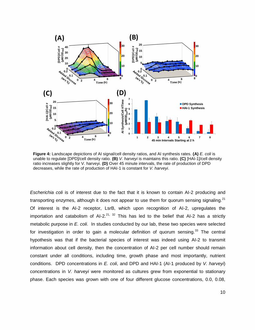
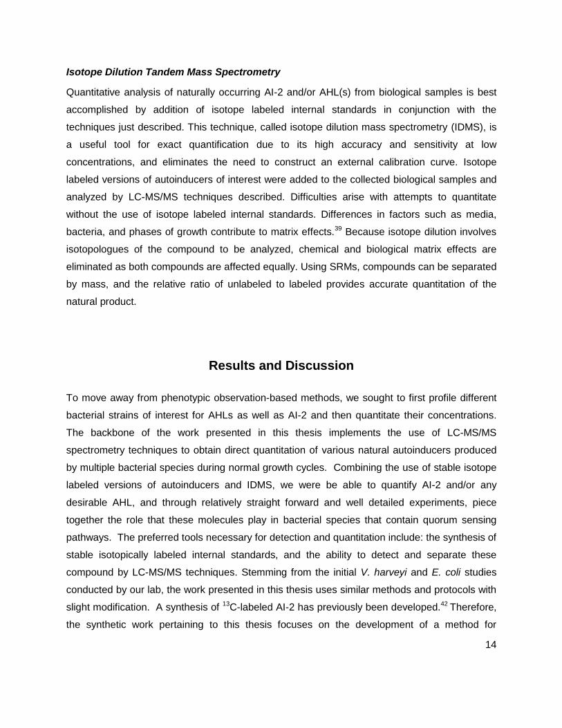
Figure 4: Landscape depictions of AI signal/cell density ratios, and AI synthesis rates. (A) E. coli is unable to regulate [DPD]/cell density ratio. (B) V. harveyi is maintains this ratio. (C) [HAI-1]/cell density ratio increases slightly for V. harveyi. (D) Over 45 minute intervals, the rate of production of DPD decreases, while the rate of production of HAI-1 is constant for V. harveyi.

0

1

2

3

4

5

6

7

1 2 3 4 5 6 7 8

AI S

yn

thesis

/Cell #

/Tim

e

(µM

/OD

600/h

)

45 min Intervals Starting at 2 h

DPD Synthesis

HAI-1 Synthesis

2 4 6 80

0.1

0.20

5

10

15

20

0

10

20

30

[HA

I-1

]/C

ell

#

(µM

/OD

600)

2 4 6 80

0.1

0.20

10

20

30

40

0

10

20

30

[DP

D]/

Cell

#

(µM

/OD

600)

2 4 6 80

0.1

0.20

5

10

15

20

0

10

20

30

[DP

D]/

Cell

#

(µM

/OD

600)

(A) (B)

(C) (D)

11

0.14, or 0.20% (w/v). As glucose concentrations increased, i.e. added nutrients increased,

neither E. coli nor V. harveyi demonstrated a considerable increase in cell density. It was found

that [DPD]/cell density in E. coli varied from 4.8 ± 0.5 to 39 ± 4.8 µM/OD600, indicating that E.

coli is not capable of regulating cell density information without regulation of metabolism (Figure

4A). Conversely, [DPD]/cell density in V. harveyi remained nearly constant under all the glucose

concentrations (Figure 4B), indicating its use as a quorum sensing signal. When [HAI-1]/cell

density was examined, the ratio did increase from 0.7 ± 0.2 to 6.6 ± 0.4 µM/OD600. (Figure 4C),

however with added glucose concentrations, [HAI-1] showed no significant changes during

exponential phase. This led us to believe that HA1-1 is not used as a quorum sensing signal in

V. harveyi. Additionally, the rate at which V. harveyi produces DPD decreased over time, while

the rate of production of HAI-1 stayed constant (Figure 4D). The initial studies of these two

species are what led to the following definition of quorum sensing33:

These studies effectively validated a method by which future studies on a wide variety of

bacteria could be studied. Using this definition of quorum sensing, [AI-2] can be quickly

screened for in various bacteria to determine if the species of interest uses AI-2 as a quorum

sensing signal.

Analytical Methods

Methods of detection for both AI-2 and AHLs have included bioassays, chromatography, and

spectrometry.6 Previously, many of the reported studies had focused on genomics and

proteomics, or the genotypic and phenotypic expression of quorum sensing-dependant

behaviors such as the observation of bioluminescence in order to detect the presence of

autoinducers in biological samples. The function of AI-2 and other autoinducers has also been

studied by constructing and utilizing luxS and other genetic mutants.

Bioassays are used mainly for detection and often rely on reporter strains to obtain

quantitation.34, 35 Several different methods of detecting and even quantifying AI-2 and AHLs

have been reported. Up until now, the most widely used method for detecting AI-2 was the V.

12

harveyi bioassay. Quantitation with this method is problematic as this method has a very small

linear range and is not very reproducible. Other problems with detecting AI-2 are that it has

many chemical forms, it degrades upon concentration and has no chromophore. In the case of

AHL detection, crucial drawbacks of bioassay methods are that sensitivity varies greatly

between different AHLs, and a different assay is needed for different species of bacteria.

Although these methods were initially useful in determining the presence of AIs, they are lacking

in the ability to produce a quantitative understanding of quorum sensing molecules. One of the

earliest quantitative methods developed was a radioactive assay in which [1-14C]-L-methionine

is incorporated into production of AHLs via SAM.36 Using this method, relative amounts of AHLs

can be quantified, however the use of [1-14C]-L-methionine is costly, and this method failed to

identify all of the AHLs previously reported for the bacteria of interest suggesting a lack of

sensitivity. Gas chromatography combined with mass spectrometry has also been implemented

for the identification and quantitation of [AHL].37, 38

High Performance Liquid Chromatography Tandem Mass Spectrometry

Profiling of AHLs have been completed using LC/MS techniques and have been successful in

establishing a methodology in which semi-quanititative information can be rapidly produced.39, 40

While our approach uses similar technology, it ultimately provides direct quantitation that

combines a number of preferred attributes not previously seen before in the field. Using high

performance liquid chromatography tandem mass spectrometry (LC-MS/MS) in conjunction with

selected reaction monitoring (SRM) produces a method that is adequately sensitive, facile and

universal. This method was first used for the detection and quantitation of [AI-2] by our lab in

the V. harveyi and E. coli experiments with good results.41 After separation by liquid

chromatography, samples can be analyzed by the method of selected reaction monitoring

events (SRM) on a triple quadrupole mass spectrometer. In this method a precursor ion of m/z

is selected in the first quadrupole. This parent ion is then fragmented by collisionally-induced

dissociation (CID) in the second quadrupole, and a characteristic fragment of the ion is selected

in the third. This allows compounds of the same mass to be separated as well as co-eluting

compounds. This method is perfectly suited for detection of AHLs as they have two specific

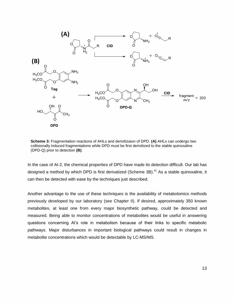
fragmentations reactions, both of which can be detected by SRM (Scheme 3A).

13

In the case of AI-2, the chemical properties of DPD have made its detection difficult. Our lab has

designed a method by which DPD is first derivatized (Scheme 3B).41 As a stable quinoxaline, it

can then be detected with ease by the techniques just described.

Another advantage to the use of these techniques is the availability of metabolomics methods

previously developed by our laboratory (see Chapter II). If desired, approximately 350 known

metabolites, at least one from every major biosynthetic pathway, could be detected and

measured. Being able to monitor concentrations of metabolites would be useful in answering

questions concerning AI’s role in metabolism because of their links to specific metabolic

pathways. Major disturbances in important biological pathways could result in changes in

metabolite concentrations which would be detectable by LC-MS/MS.

(A)

(B)

Scheme 3: Fragmentation reactions of AHLs and derivitizaion of DPD. (A) AHLs can undergo two collisionally induced fragmentations while DPD must be first derivitized to the stable quinoxaline

(DPD-Q) prior to detection (B).

14

Isotope Dilution Tandem Mass Spectrometry

Quantitative analysis of naturally occurring AI-2 and/or AHL(s) from biological samples is best

accomplished by addition of isotope labeled internal standards in conjunction with the

techniques just described. This technique, called isotope dilution mass spectrometry (IDMS), is

a useful tool for exact quantification due to its high accuracy and sensitivity at low

concentrations, and eliminates the need to construct an external calibration curve. Isotope

labeled versions of autoinducers of interest were added to the collected biological samples and

analyzed by LC-MS/MS techniques described. Difficulties arise with attempts to quantitate

without the use of isotope labeled internal standards. Differences in factors such as media,

bacteria, and phases of growth contribute to matrix effects.39 Because isotope dilution involves

isotopologues of the compound to be analyzed, chemical and biological matrix effects are

eliminated as both compounds are affected equally. Using SRMs, compounds can be separated

by mass, and the relative ratio of unlabeled to labeled provides accurate quantitation of the

natural product.

Results and Discussion

To move away from phenotypic observation-based methods, we sought to first profile different

bacterial strains of interest for AHLs as well as AI-2 and then quantitate their concentrations.

The backbone of the work presented in this thesis implements the use of LC-MS/MS

spectrometry techniques to obtain direct quantitation of various natural autoinducers produced

by multiple bacterial species during normal growth cycles. Combining the use of stable isotope

labeled versions of autoinducers and IDMS, we were be able to quantify AI-2 and/or any

desirable AHL, and through relatively straight forward and well detailed experiments, piece

together the role that these molecules play in bacterial species that contain quorum sensing

pathways. The preferred tools necessary for detection and quantitation include: the synthesis of

stable isotopically labeled internal standards, and the ability to detect and separate these

compound by LC-MS/MS techniques. Stemming from the initial V. harveyi and E. coli studies

conducted by our lab, the work presented in this thesis uses similar methods and protocols with

slight modification. A synthesis of 13C-labeled AI-2 has previously been developed.42 Therefore,

the synthetic work pertaining to this thesis focuses on the development of a method for

15

detecting and quantitating AHLs, although the bacterial species studied were indeed profiled for

both AI-2 and AHLs. A logical design for the synthesis of doubly deuterated AHLs was proposed

and completed, and these molecules have been implemented in several biological studies.

Further, chromatographic and spectrometric techniques for the detection of AI-2 have been

improved. Methods for AHLs have been developed and refined to the point that future

experiments can be executed with ease.

Design Rationale for the Synthesis of Stable Isotope Labeled AHLs

There were several specific goals when we considered the synthesis of stable isotope labeled

AHLs. In order to easily produce any AHL desirable with minimal steps, the isotope should be

incorporated in the conserved part of the molecule, in this case, the lactone ring. Additionally,

the use of two deuteriums, as opposed to the use of one, allows the resulting internal standard

to be distinguishable from the appearance of a natural 13C isotopomer. The next objective was

to easily and effectively produce all AHLs by using solid phase synthesis techniques. The

reason for the use of solid phase chemistry was to increase yields and eliminate the need for

further purification. Using this technique also enables the synthesis to be biomimetic. The

proposed synthesis should have also yielded an enantiomerically pure product, which would

further reduce the chance of the occurrence of matrix effects leading to invalid measurements.

Although N-acyl-homoserine lactones have been made previously, most reports have either

used synthetic C7AHL as reference compound, as it is not thought to be biologically present in

most systems,38 or incorporated a 13C into the acyl chain.43 A synthesis of tetra-deuterated acyl-

homoserine lactones has been reported44, however this synthesis did not take advantage of

solid phase techniques, and therefore required extensive purification of both intermediates and

AHLs.

Synthesis of Deuterated N-Acyl Homoserine Lactones

In order to implement the chosen method of incorporating any acyl chain into AHLs by use of

solid phase chemistry, we determined that (S)-[4,4,2H2]-N-Fmoc-methionine 6 would be a useful

common intermediate. Synthesis of 6 began with protected aspartic acid derivative, 1. This

molecule was synthesized by a series of known steps.45 Protecting groups were chosen by

16

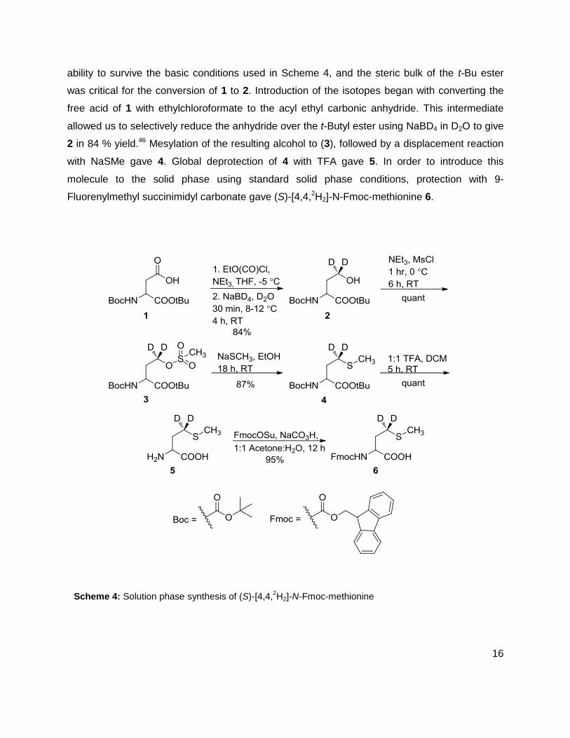
ability to survive the basic conditions used in Scheme 4, and the steric bulk of the t-Bu ester

was critical for the conversion of 1 to 2. Introduction of the isotopes began with converting the

free acid of 1 with ethylchloroformate to the acyl ethyl carbonic anhydride. This intermediate

allowed us to selectively reduce the anhydride over the t-Butyl ester using NaBD4 in D2O to give

2 in 84 % yield.46 Mesylation of the resulting alcohol to (3), followed by a displacement reaction

with NaSMe gave 4. Global deprotection of 4 with TFA gave 5. In order to introduce this

molecule to the solid phase using standard solid phase conditions, protection with 9-

Fluorenylmethyl succinimidyl carbonate gave (S)-[4,4,2H2]-N-Fmoc-methionine 6.

Scheme 4: Solution phase synthesis of (S)-[4,4,2H2]-N-Fmoc-methionine

17

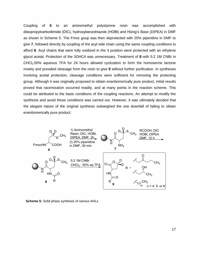
Coupling of 6 to an aminomethyl polystyrene resin was accomplished with

diisopropylcarbodiimide (DIC), hydroxybenzotriazole (HOBt) and Hünig’s Base (DIPEA) in DMF

as shown in Scheme 5. The Fmoc goup was then deprotected with 25% piperidine in DMF to

give 7, followed directly by coupling of the acyl side chain using the same coupling conditions to

afford 8. Acyl chains that were fully oxidized in the 3 position were protected with an ethylene

glycol acetal. Protection of the 3OHC4 was unnecessary. Treatment of 8 with 5:2 1M CNBr in

CHCl3:50% aqueous TFA for 24 hours allowed cyclization to form the homoserine lactone

moiety and provided cleavage from the resin to give 9 without further purification. In syntheses

involving acetal protection, cleavage conditions were sufficient for removing the protecting

group. Although it was originally proposed to obtain enantiomerically pure product, initial results

proved that racemization occurred readily, and at many points in the reaction scheme. This

could be attributed to the basic conditions of the coupling reactions. An attempt to modify the

synthesis and avoid these conditions was carried out. However, it was ultimately decided that

the elegant nature of the original synthesis outweighed the one downfall of failing to obtain

enantiomerically pure product.

Scheme 5: Solid phase synthesis of various AHLs

18

Separation and Detection of AHLs and AI-2

As previously stated, the chemical properties of DPD and its various active forms have made its

detection problematic. A simple derivatization, developed by our lab,41 allows such

complications to be avoided. Although it was not an initial focus of this project, a shorter 4 min

LC-MS/MS method was developed for the quantitation of AI-2. Using this isocratic gradient, the

throughput for the analysis of biological samples was subsequently increased. Previous

methods for AHL separation have been long, ranging from ~30-50 minutes.45, 47 Two shorter

methods have been reported40, although these methods used high column temperatures or

atypical additives in the mobile phase such as ethylenediaminetetraaceticacid (EDTA).48 These

conditions are often not suitable for most LC-MS methods. To ensure a high throughput for the

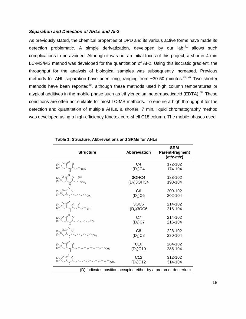
detection and quantitation of multiple AHLs, a shorter, 7 min, liquid chromatography method

was developed using a high-efficiency Kinetex core-shell C18 column. The mobile phases used

Table 1: Structure, Abbreviations and SRMs for AHLs

Structure Abbreviation SRM

Parent-fragment (m/z-m/z)

C4 (D2)C4

172-102 174-104

3OHC4 (D2)3OHC4

188-102 190-104

C6 (D2)C6

200-102 202-104

3OC6 (D2)3OC6

214-102 216-104

C7 (D2)C7

214-102 216-104

C8 (D2)C8

228-102 230-104

C10 (D2)C10

284-102 286-104

C12 (D2)C12

312-102 314-104

(D) indicates position occupied either by a proton or deuterium

19

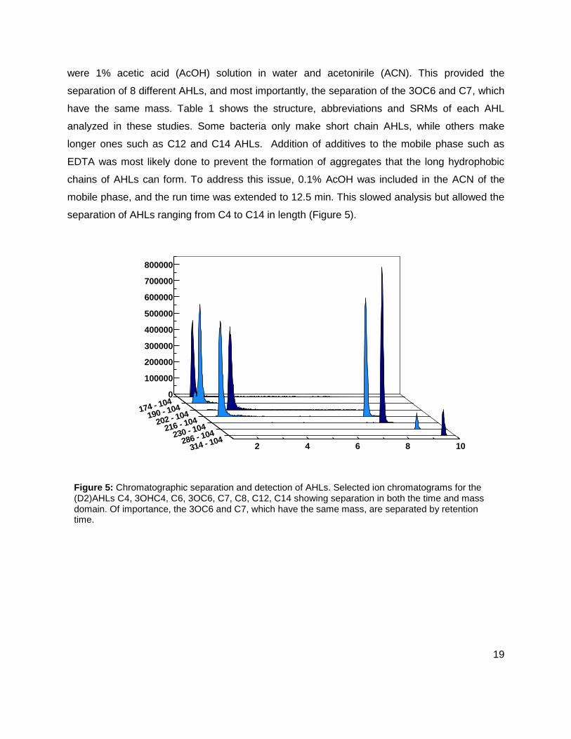
were 1% acetic acid (AcOH) solution in water and acetonirile (ACN). This provided the

separation of 8 different AHLs, and most importantly, the separation of the 3OC6 and C7, which

have the same mass. Table 1 shows the structure, abbreviations and SRMs of each AHL

analyzed in these studies. Some bacteria only make short chain AHLs, while others make

longer ones such as C12 and C14 AHLs. Addition of additives to the mobile phase such as

EDTA was most likely done to prevent the formation of aggregates that the long hydrophobic

chains of AHLs can form. To address this issue, 0.1% AcOH was included in the ACN of the

mobile phase, and the run time was extended to 12.5 min. This slowed analysis but allowed the

separation of AHLs ranging from C4 to C14 in length (Figure 5).

Figure 5: Chromatographic separation and detection of AHLs. Selected ion chromatograms for the (D2)AHLs C4, 3OHC4, C6, 3OC6, C7, C8, C12, C14 showing separation in both the time and mass domain. Of importance, the 3OC6 and C7, which have the same mass, are separated by retention time.

0

100000

200000

300000

400000

500000

600000

700000

800000

174 - 104

190 - 104

202 - 104

216 - 104

230 - 104

286 - 104

314 - 1042 4 6 8 10

20

Profiling Bacterial Species for Autoinducer Production

There are a variety of species of bacteria known to produce AI-1s and AI-2. Table 2 summarizes

the strains that have been profiled as well as which have been profiled for AHLs and/or AI-2.

These species were selected for analysis based on whether they possess a LuxS or LuxI

homologue, availability, as well as the ability to grow them in the lab. Two wild type strains of

Vibrio fischeri have been profiled for both AI-2 and AHL production. The ainS mutant of Vibrio

fischeri, CL21, which lacks the ability to produce the C8 AHL as well as VCW2G7, the LuxI

mutant of ES114 were profiled for AHL production. Again, LuxI is responsible for producing the

3OC6 AHL; therefore, this mutant lacks the ability to produce the 3OC6 AHL. Ralstonia pickettii

(data not shown), Edwarseilla tarda and Yersinia enterocolitica have all been profiled for AI-2

production. In each of these studies, AI production was monitored as cultures grew from

exponential to stationary phase. Optical density was taken for each culture to measure growth,

and cultures were studied with added glucose concentrations of 0, 0.08, 0.14 % (w/v), or a

combination of these. Measured concentrations of AI-2 and AHLs are denoted as [DPD] and

[AHL(s)], respectively.

Table 2: Strains Profiled

Organism Strain Genotype AI-1s AI-2

Edwardsiella tarda 15947 WT

Vibrio fischeri MJ-1 WT

Vibrio fischeri ES114 WT

Vibrio fischeri VCW2G7 luxI-

Vibrio fischeri CL21 ainS-

Ralstonia pickettii 49129 WT -

Yersinia enterocolitica 9610 WT

WT = wild type

21

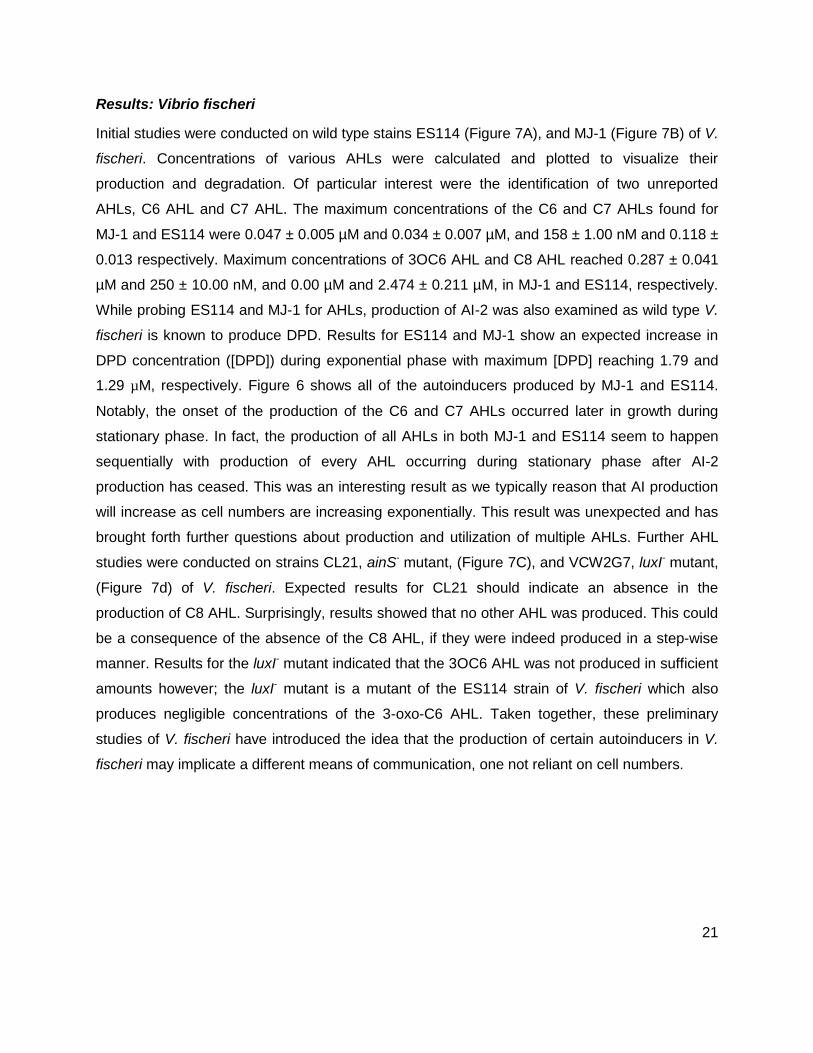
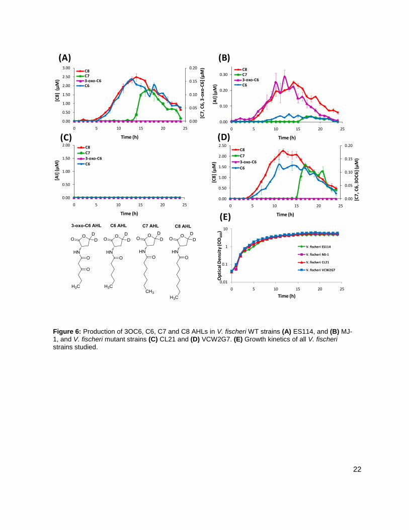
Results: Vibrio fischeri

Initial studies were conducted on wild type stains ES114 (Figure 7A), and MJ-1 (Figure 7B) of V.

fischeri. Concentrations of various AHLs were calculated and plotted to visualize their

production and degradation. Of particular interest were the identification of two unreported

AHLs, C6 AHL and C7 AHL. The maximum concentrations of the C6 and C7 AHLs found for

MJ-1 and ES114 were 0.047 ± 0.005 µM and 0.034 ± 0.007 µM, and 158 ± 1.00 nM and 0.118 ±

0.013 respectively. Maximum concentrations of 3OC6 AHL and C8 AHL reached 0.287 ± 0.041

µM and 250 ± 10.00 nM, and 0.00 µM and 2.474 ± 0.211 µM, in MJ-1 and ES114, respectively.

While probing ES114 and MJ-1 for AHLs, production of AI-2 was also examined as wild type V.

fischeri is known to produce DPD. Results for ES114 and MJ-1 show an expected increase in

DPD concentration ([DPD]) during exponential phase with maximum [DPD] reaching 1.79 and

1.29 µM, respectively. Figure 6 shows all of the autoinducers produced by MJ-1 and ES114.

Notably, the onset of the production of the C6 and C7 AHLs occurred later in growth during

stationary phase. In fact, the production of all AHLs in both MJ-1 and ES114 seem to happen

sequentially with production of every AHL occurring during stationary phase after AI-2

production has ceased. This was an interesting result as we typically reason that AI production

will increase as cell numbers are increasing exponentially. This result was unexpected and has

brought forth further questions about production and utilization of multiple AHLs. Further AHL

studies were conducted on strains CL21, ainS- mutant, (Figure 7C), and VCW2G7, luxI- mutant,

(Figure 7d) of V. fischeri. Expected results for CL21 should indicate an absence in the

production of C8 AHL. Surprisingly, results showed that no other AHL was produced. This could

be a consequence of the absence of the C8 AHL, if they were indeed produced in a step-wise

manner. Results for the luxI- mutant indicated that the 3OC6 AHL was not produced in sufficient

amounts however; the luxI- mutant is a mutant of the ES114 strain of V. fischeri which also

produces negligible concentrations of the 3-oxo-C6 AHL. Taken together, these preliminary

studies of V. fischeri have introduced the idea that the production of certain autoinducers in V.

fischeri may implicate a different means of communication, one not reliant on cell numbers.

22

Figure 6: Production of 3OC6, C6, C7 and C8 AHLs in V. fischeri WT strains (A) ES114, and (B) MJ-1, and V. fischeri mutant strains (C) CL21 and (D) VCW2G7. (E) Growth kinetics of all V. fischeri strains studied.

0.00

0.05

0.10

0.15

0.20

0.00

0.50

1.00

1.50

2.00

2.50

3.00

0 5 10 15 20 25

[C7

, C6

, 3-o

xo-C

6] (

µM

)

[C8

] (

µM

)

Time (h)

C8C73-oxo-C6C6

0.00

0.10

0.20

0.30

0 5 10 15 20 25

[AI]

(µM

)

Time (h)

C8C73-oxo-C6C6

0.00

0.50

1.00

1.50

2.00

0 5 10 15 20 25

[AI]

(µ

M)

Time (h)

C8

C7

3-oxo-C6

C6

0.00

0.05

0.10

0.15

0.20

0.00

0.50

1.00

1.50

2.00

2.50

0 5 10 15 20 25

[C7

, C6

, 3O

C6

] (µ

M)

[C8

] (µ

M)

Time (h)

C8

C7

3-oxo-C6

C6

0.01

0.1

1

10

0 5 10 15 20 25

Op

tica

l De

nsi

ty (O

D6

00)

Time (h)

V. fischeri ES114

V. fischeri MJ-1

V. fischeri CL21

V. fischeri VCW2G7

(A) (B)

(C) (D)

(E)

23

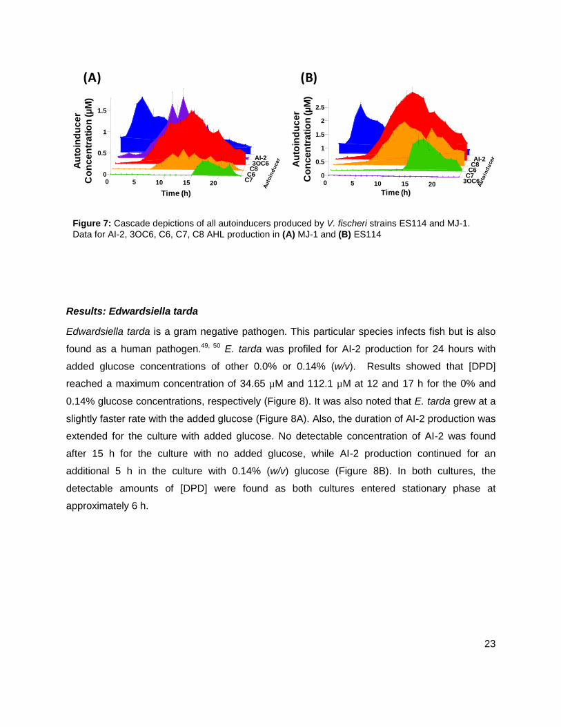
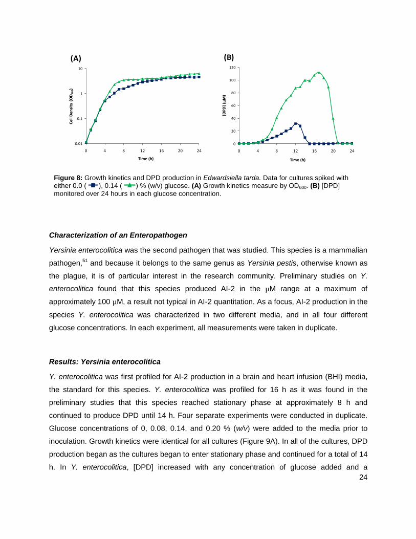
Results: Edwardsiella tarda

Edwardsiella tarda is a gram negative pathogen. This particular species infects fish but is also

found as a human pathogen.49, 50 E. tarda was profiled for AI-2 production for 24 hours with

added glucose concentrations of other 0.0% or 0.14% (w/v). Results showed that [DPD]

reached a maximum concentration of 34.65 µM and 112.1 µM at 12 and 17 h for the 0% and

0.14% glucose concentrations, respectively (Figure 8). It was also noted that E. tarda grew at a

slightly faster rate with the added glucose (Figure 8A). Also, the duration of AI-2 production was

extended for the culture with added glucose. No detectable concentration of AI-2 was found

after 15 h for the culture with no added glucose, while AI-2 production continued for an

additional 5 h in the culture with 0.14% (w/v) glucose (Figure 8B). In both cultures, the

detectable amounts of [DPD] were found as both cultures entered stationary phase at

approximately 6 h.

Figure 7: Cascade depictions of all autoinducers produced by V. fischeri strains ES114 and MJ-1.

Data for AI-2, 3OC6, C6, C7, C8 AHL production in (A) MJ-1 and (B) ES114

Time (h)

Au

toin

du

ce

r

Co

nc

en

tra

tio

n (µ

M)

0 5 10 15 20C7C6C83OC6AI-2

0

0.5

1

1.5

0 5 10 15 203OC6C7C6C8AI-2

0

0.5

1

1.5

2

2.5

0 5 10 15 203OC6C7C6C8AI-2

0

0.5

1

1.5

2

2.5

0 5 10 15 203OC6C7C6C8AI-2

0

0.5

1

1.5

2

2.5

0

5

10

15

20

3OC6

C7C

6C8A

I-2

0

0.5

1

1.5

2

2.5

Time (h)

Au

toin

du

ce

r

Co

nc

en

tra

tio

n (µ

M)

(A) (B)

24

Characterization of an Enteropathogen

Yersinia enterocolitica was the second pathogen that was studied. This species is a mammalian

pathogen,51 and because it belongs to the same genus as Yersinia pestis, otherwise known as

the plague, it is of particular interest in the research community. Preliminary studies on Y.

enterocolitica found that this species produced AI-2 in the µM range at a maximum of

approximately 100 µM, a result not typical in AI-2 quantitation. As a focus, AI-2 production in the

species Y. enterocolitica was characterized in two different media, and in all four different

glucose concentrations. In each experiment, all measurements were taken in duplicate.

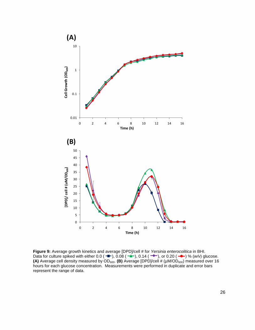
Results: Yersinia enterocolitica

Y. enterocolitica was first profiled for AI-2 production in a brain and heart infusion (BHI) media,

the standard for this species. Y. enterocolitica was profiled for 16 h as it was found in the

preliminary studies that this species reached stationary phase at approximately 8 h and

continued to produce DPD until 14 h. Four separate experiments were conducted in duplicate.

Glucose concentrations of 0, 0.08, 0.14, and 0.20 % (w/v) were added to the media prior to

inoculation. Growth kinetics were identical for all cultures (Figure 9A). In all of the cultures, DPD

production began as the cultures began to enter stationary phase and continued for a total of 14

h. In Y. enterocolitica, [DPD] increased with any concentration of glucose added and a

Figure 8: Growth kinetics and DPD production in Edwardsiella tarda. Data for cultures spiked with either 0.0 ( ), 0.14 ( ) % (w/v) glucose. (A) Growth kinetics measure by OD600. (B) [DPD] monitored over 24 hours in each glucose concentration.

0

5

10

15

20

25

30

35

40

45

50

0 2 4 6 8 10 12 14 16

[DP

D]/

cell

# (u

M/O

D6

00)

Time (h)

Average [DPD]/OD 0.0% glucose





Average [DPD]/OD 0.50% glucose0

5

10

15

20

25

30

35

40

45

50

0 2 4 6 8 10 12 14 16

[DP

D]/

cell

# (u

M/O

D60

0)

Time (h)







0.01

0.1

1

10

0 4 8 12 16 20 24

Ce

ll D

en

sity

(O

D60

0)

Time (h)

(A)

0

20

40

60

80

100

120

0 4 8 12 16 20 24

[DP

D]

(µM

)

Time (h)

(B)

25

maximum concentration of 115.12 ± 4.09 µM DPD was found at 12 h. Concentrations of DPD in

the 0.0 % glucose culture reached a maximum of 78.62 ± 0.24 µM. The maximum [DPD]/OD600

in all of the glucose concentrations was relatively small range, from 28.75 ± 0.54 µM to 36.54 ±

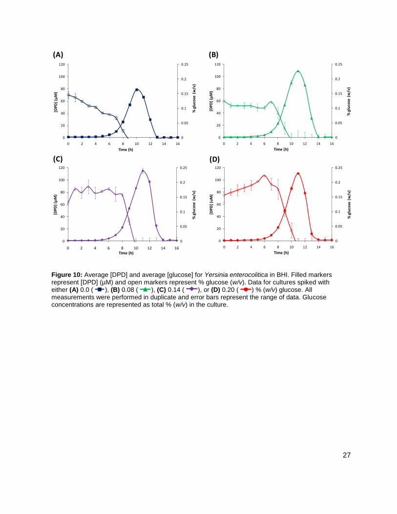
0.39 µM (Figure 9B). Results from the colorimetric glucose oxidation assay revealed that

glucose levels in each culture dissipated to 0 % over the course of ~2-3 h during the time that

[DPD] were increasing (Figure 10A-D). These data seemed to indicate that a Y. enterocolitica

reached a maximum [DPD] with any concentration of added nutrients. Because BHI contains 3

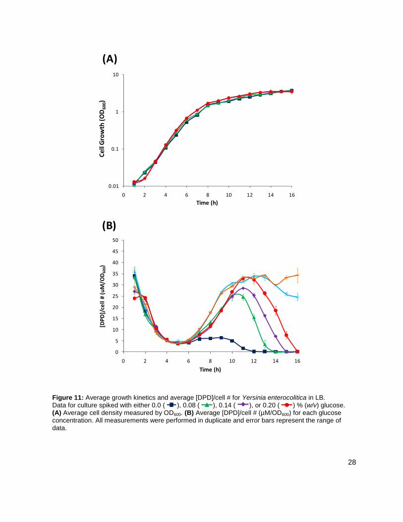
g glucose per 1 L, it was attempted to repeat these experiments, with the same conditions, in a

medium that contained low glucose and sugar carbon sources such as LB. Results, as

indicated by measurement of OD600 showed that Y. enterocolitica grew similarly in LB as in BHI

(Figure 11A). When experiments were repeated with identical glucose concentrations, it was

noted that the [DPD]/OD600 increased both in maximum amount and with time as glucose

concentrations increased as shown in Figure 11B. Again, DPD production began as Y.

enterocolitica entered stationary phase. In the 0.0 % (w/v) glucose culture, the [DPD]/OD600

reached a maximum of 6.391 ± 0.380 µM at 8 h; the 0.08 % (w/v) glucose culture reached a

maximum the [DPD]/OD600 of 25.11 ± 2.203 µM at 9 h; the 0.14 % (w/v) glucose culture

reached a maximum the [DPD]/OD600 of 28.56 ± 0.069 µM at 10 h; and the 0.08 % (w/v) glucose

culture reached a maximum the [DPD]/OD600 of 32.92 ± 1.115 µM at 11 h. Two additional

glucose concentrations were used in the LB studies in an attempt to locate a threshold

concentration at which Y. enterocolitica would produce a maximum [DPD].

26

Figure 9: Average growth kinetics and average [DPD]/cell # for Yersinia enterocolitica in BHI. Data for culture spiked with either 0.0 ( ), 0.08 ( ), 0.14 ( ), or 0.20 ( ) % (w/v) glucose. (A) Average cell density measured by OD600. (B) Average [DPD]/cell # (µM/OD600) measured over 16 hours for each glucose concentration. Measurements were performed in duplicate and error bars represent the range of data.

0

5

10

15

20

25

30

35

40

45

50

0 2 4 6 8 10 12 14 16

[DP

D]/

cell

# (u

M/O

D6

00)

Time (h)







5

10

15

20

25

30

35

40

45

50

0 2 4 6 8 10 12 14 16

[DP

D]/

cell

# (u

M/O

D60

0)

Time (h)







0

5

10

15

20

25

30

35

40

45

50

0 2 4 6 8 10 12 14 16

[DPD

]/ce

ll #

(uM

/OD

600)

Time (h)







0

5

10

15

20

25

30

35

40

45

50

0 2 4 6 8 10 12 14 16

[DPD

]/ce

ll #

(uM

/OD

600)

Time (h)







0

5

10

15

20

25

30

35

40

45

50

0 2 4 6 8 10 12 14 16

[DP

D]/

ce

ll #

(uM

/OD

60

0)

Time (h)

(B)

(A)

0.01

0.1

1

10

0 2 4 6 8 10 12 14 16

Ce

ll G

row

th (

OD

600)

Time (h)

27

0

0.05

0.1

0.15

0.2

0.25

0

20

40

60

80

100

120

0 2 4 6 8 10 12 14 16

% g

luco

se (

w/v

)

[DP

D]

(µM

)

Time (h)

0

0.05

0.1

0.15

0.2

0.25

0

20

40

60

80

100

120

0 2 4 6 8 10 12 14 16

% g

luco

se (

w/v

)

[DP

D]

(µM

)

Time (h)

0

0.05

0.1

0.15

0.2

0.25

0

20

40

60

80

100

120

0 2 4 6 8 10 12 14 16

% g

luco

se (

w/v

)

[DP

D]

(µM

)

Time (h)

0

0.05

0.1

0.15

0.2

0.25

0

20

40

60

80

100

120

0 2 4 6 8 10 12 14 16

% g

luco

se (

w/v

)

[DP

D]

(uM

)

Time (h)

(A) (B)

(C) (D)

Figure 10: Average [DPD] and average [glucose] for Yersinia enterocolitica in BHI. Filled markers represent [DPD] (µM) and open markers represent % glucose (w/v). Data for cultures spiked with either (A) 0.0 ( ), (B) 0.08 ( ), (C) 0.14 ( ), or (D) 0.20 ( ) % (w/v) glucose. All measurements were performed in duplicate and error bars represent the range of data. Glucose concentrations are represented as total % (w/v) in the culture.

0

5

10

15

20

25

30

35

40

45

50

0 2 4 6 8 10 12 14 16

[DP

D]/

cell

# (u

M/O

D6

00)

Time (h)







5

10

15

20

25

30

35

40

45

50

0 2 4 6 8 10 12 14 16

[DP

D]/

cell

# (u

M/O

D60

0)

Time (h)







0

5

10

15

20

25

30

35

40

45

50

0 2 4 6 8 10 12 14 16

[DPD

]/ce

ll #

(uM

/OD

600)

Time (h)







0

5

10

15

20

25

30

35

40

45

50

0 2 4 6 8 10 12 14 16

[DPD

]/ce

ll #

(uM

/OD

600)

Time (h)







28

0

5

10

15

20

25

30

35

40

45

50

0 2 4 6 8 10 12 14 16

[DP

D]/

cell

# (u

M/O

D6

00)

Time (h)

(B)

(A)

0.01

0.1

1

10

0 2 4 6 8 10 12 14 16

Cel

l Gro

wth

(O

D60

0)

Time (h)

Figure 11: Average growth kinetics and average [DPD]/cell # for Yersinia enterocolitica in LB. Data for culture spiked with either 0.0 ( ), 0.08 ( ), 0.14 ( ), or 0.20 ( ) % (w/v) glucose. (A) Average cell density measured by OD600. (B) Average [DPD]/cell # (µM/OD600) for each glucose concentration. All measurements were performed in duplicate and error bars represent the range of data.

0

5

10

15

20

25

30

35

40

45

50

0 2 4 6 8 10 12 14 16

[DP

D]/

cell

# (u

M/O

D6

00)

Time (h)







5

10

15

20

25

30

35

40

45

50

0 2 4 6 8 10 12 14 16

[DP

D]/

cell

# (u

M/O

D60

0)

Time (h)







0

5

10

15

20

25

30

35

40

45

50

0 2 4 6 8 10 12 14 16

[DPD

]/ce

ll #

(uM

/OD

600)

Time (h)







0

5

10

15

20

25

30

35

40

45

50

0 2 4 6 8 10 12 14 16

[DPD

]/ce

ll #

(uM

/OD

600)

Time (h)







29

0

0.05

0.1

0.15

0.2

0.25

0

20

40

60

80

100

120

0 2 4 6 8 10 12 14 16

% g

luco

se (

w/v

)

[DP

D]

(µM

)

Time (h)

0

0.05

0.1

0.15

0.2

0.25

0

20

40

60

80

100

120

0 2 4 6 8 10 12 14 16

% g

luco

se (

w/v

)

[DP

D]

(µM

)

Time (h)

0

0.05

0.1

0.15

0.2

0.25

0

20

40

60

80

100

120

0 2 4 6 8 10 12 14 16

% g

luco

se (

w/v

)

[DP

D]

(µM

)

Time (h)

0

0.05

0.1

0.15

0.2

0.25

0

20

40

60

80

100

120

0 2 4 6 8 10 12 14 16

% g

luco

se (

w/v

)

[DP

D]

(µM

)

Time (h)

0

0.05

0.1

0.15

0.2

0.25

0

20

40

60

80

100

120

0 2 4 6 8 10 12 14 16

% g

luco

se (

w/v

)

[DP

D]

(µM

)

Time (h)

0

0.05

0.1

0.15

0.2

0.25

0

20

40

60

80

100

120

140

0 2 4 6 8 10 12 14 16

% g

luco

se (

w/v

)

[DP

D]

(µM

)

Time (h)

(A) (B)

(C) (D)

(E) (F)

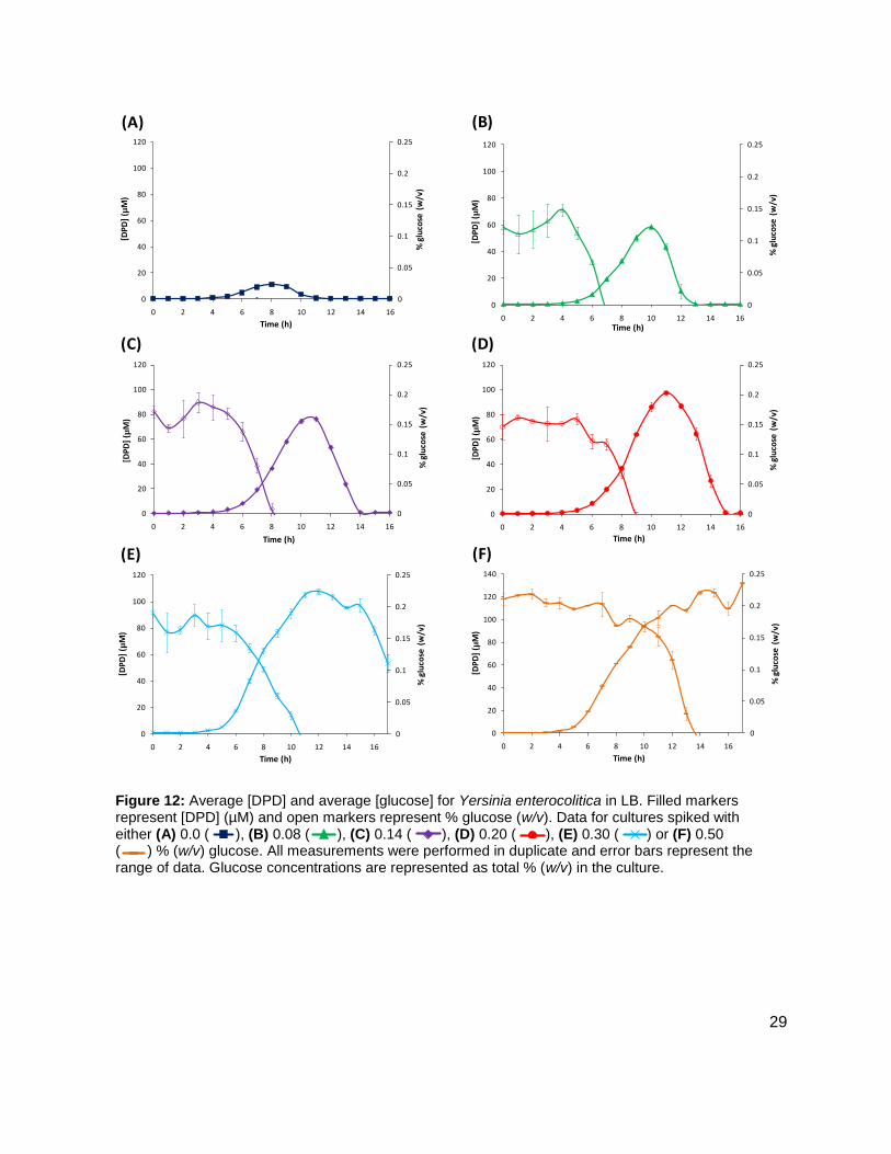
Figure 12: Average [DPD] and average [glucose] for Yersinia enterocolitica in LB. Filled markers represent [DPD] (µM) and open markers represent % glucose (w/v). Data for cultures spiked with either (A) 0.0 ( ), (B) 0.08 ( ), (C) 0.14 ( ), (D) 0.20 ( ), (E) 0.30 ( ) or (F) 0.50 ( ) % (w/v) glucose. All measurements were performed in duplicate and error bars represent the range of data. Glucose concentrations are represented as total % (w/v) in the culture.

0

5

10

15

20

25

30

35

40

45

50

0 2 4 6 8 10 12 14 16

[DP

D]/

cell

# (u

M/O

D6

00)

Time (h)







0

5

10

15

20

25

30

35

40

45

50

0 2 4 6 8 10 12 14 16

[DP

D]/

cell

# (u

M/O

D60

0)

Time (h)







0

5

10

15

20

25

30

35

40

45

50

0 2 4 6 8 10 12 14 16

[DP

D]/

cell

# (u

M/O

D60

0)

Time (h)







0

5

10

15

20

25

30

35

40

45

50

0 2 4 6 8 10 12 14 16

[DPD

]/ce

ll #

(uM

/OD

600)

Time (h)







0

5

10

15

20

25

30

35

40

45

50

0 2 4 6 8 10 12 14 16

[DPD

]/ce

ll #

(uM

/OD

600)

Time (h)







5

10

15

20

25

30

35

40

45

50

0246810121416

[DPD]/cell # (uM/OD

600 )

Time (h)







30

Methods and Materials

General Methods

Optical densities were measured on a BioPhotometer (Eppendorf), and all absorbance

measurements for the colorimetric glucose oxidase assay were performed on a µQUANT

Universal Microplate Spectrophotometer (Bio-Tek Instruments, Inc.). The liquid

chromatography-tandem mass spectrometer (LC-MS/MS) used for detection of both AI-2 and

AHLs consisted of a Thermo Electron Surveyor Autosampler Plus, a Surveyor MS Pump Plus,

and a TSQ Quantum Discovery Max triple quadrupole MS. All separations were performed on a

Kinetex reverse phase C18 core-shell column (5 µm pore size, 100 Ǻ particle size, 100 x 2 mm)

supplied by Phenomenex. All MS spectra were collected and analyzed using the Xcalibur MS v

2.0.7 software package (Thermo Electron Corporation). All chemicals and solvents were

purchased from Fisher Scientific, VWR, or Chem Impex and were used without further

purification. Deuterated solvents used for NMR analysis were purchased from Cambridge

Isotope Laboratories, Inc. Silica gel (230 x 400 mesh) and TLC plates were purchased from

Sorbent Technologies. All NMR spectra were recorded on either a Varian Mercury 300 MHz, or

Varian INOVA 500 MHz spectrometer. All high accuracy mass spectra were taken on a JEOL

AccuTOF mass spectrometer with a DART ion source. IR spectra were recorded on a Thermo

Electron Nicolet IR 100 FT-IR.

Bacterial Growth Conditions

Cultures of Vibrio fischeri wild type strains ES114 and MJ-1, as well as cultures of mutant

strains CL21 and VCW2G7 were grown aerobically in Luria marine medium (LM)22 at 25 °C with

shaking. Edwardsiella tarda cultures were grown aerobically in Luria broth (LB)52 at 28 °C with

shaking. Yersinia enterocolitica cultures were grown aerobically in either LB or Brain Heart

Infusion (BHI)53 at 28 °C with shaking.

Chromatographic Details

For all samples, 10 µL was injected onto the column via delivery by autosampler. The column

temperature was 25 °C. High performance liquid chromatography (HPLC) was performed

31

utilizing a quaternary pump to generate a gradient for the elution of compounds from the

stationary phase as listed below:

AI-2

A flow rate of 200 µL/min was used. The mobile phases were 0.1% acetic acid in water (solvent

A) and HPLC grade acetonitrile (solvent B) and a 4 min isocratic method was created using 5%

solvent A, and 95% solvent B.

AHL(s)

A flow rate of 200 µL/min was used. The mobile phases used were 0.1% Acetic Acid in water

(solvent A) and HPLC grade Acetonitrile (solvent B). These were used to develop the following

12.5 minute gradient elution profile: t = 0 min, 99% solvent A, 1% solvent B; t = 0.5 min, 95%

solvent A, 5% solvent B; t = 3 min, 90% solvent A, 10% solvent B; t = 5 min, 25% solvent A,

75% solvent B; t = 6 min, 25% solvent A, 75% solvent B; t = 6.5 min, 99% solvent A, 1%

solvent B; t = 7 min, 99% solvent A, 1% solvent B.

General Mass Spectrometric Detection Parameters for AI-2 and AHLs

After delivery by HPLC, samples were introduced into the electrospray ionization chamber (ESI)

through a 0.1 mm diameter fused silica capillary. The voltage for the ESI source was set to 4500

V. Detection of both AI-2 and AHL(s) occurred in positive mode. Nitrogen was used as the

sheath gas (40 psi) and the inlet capillary temperature was 290 °C. Argon was used in the

second quadrupole as the collision gas at a pressure of 1.5 mTorr. Samples were analyzed

using selected reaction monitoring (SRM) with a scan time set to 0.05 s and a scan width of 1

m/z.

Measurement of AI-2 Concentration [AI-2]

In each experiment, the AI-2 concentration ([AI-2]) was measured as cultures grew from

exponential phase through stationary phase. A preliminary growth curve was constructed in

order to determine the time needed to reach stationary phase and cell density was measured by

optical density at 600 nm (OD600). Once determined, the following procedure was used for each

biological experiment conducted with limited modification necessary. Incubation temperature,

32

growth medium, and duration of the experiment varied with the bacteria. Cell cultures were

grown in duplicate. Incubation temperature, growth medium, and duration of the experiment

varied with the bacteria. Cell cultures were grown in duplicate, unless otherwise noted. Every

hour, a 300 µL sample was taken from each culture and placed into a 1.5 mL microcentrifuge

tube containing 10 µL a solution of 13C-DPD (341 µM). The contents were then mixed

thoroughly by vortexing and centrifuged to remove cells and other particulates. A portion of the

supernatants (260 µL) were placed in a subsequent microcentrifuge tube containing 26 µL of

DPD-Tag (5 mg/mL). The contents were allowed to react for 45 minutes before extraction with

ethyl acetate (2 x 130 µL), followed directly by LC-MS/MS analysis.

Measurement of AHL Concentration(s) [AHL(s)]

In each experiment, the AHL concentration ([AHL]) was measured as cultures grew from

exponential phase through stationary phase. A preliminary growth curve was constructed in

order to determine the time needed to reach stationary phase and cell density was measured by

OD600. Once determined, the following procedure was used for each biological experiment

conducted with limited modification necessary. Incubation temperature, growth medium, and

duration of the experiment varied with the bacteria. Cell cultures were grown in duplicate. Every

hour, a 300 µL sample was taken from each culture and placed into a 1.5 mL microcentrifuge

containing 10 µL of a solution of respective deuterated AHLs (6.2 µM). The contents were mixed

thoroughly by vortexing and centrifuged to remove cells and other particulates. The resulting

supernatants (260 µL) were extracted two times with half volume of ethyl acetate and

transferred to 300 µL autosampler vials. If an extraction could not be performed, supernatants

were taken directly after centrifugation for analysis.

Data Handling for the Calculation of [DPD]

Data from the SRMs 381-202 and 382-203 (parent-product ion) at a collision energy of 41 eV

were selected and analyzed by manual integration of chromatographic peak area to obtain

[DPD]. The SRM 381-202 and 382-203 corresponds to the DPD-Quinoxalines, (12C)DPD-Q and

(13C)DPD-Q signal respectively. One of two correction factors was applied to integration values

based on the ratio of (12C)DPD-Q to (13C)DPD-Q signal and are stated below. A full discussion

of these correction types has been previously reported by our lab.41

33

Correction type 1 is a correction for the naturally occurring (13C)DPD and was applied when the

ratio of (12C)DPD-Q to (13C)DPD-Q signal was greater than 0.3:

( ) ( ) ( )

Correction type 2 is correction for (12C)DPD impurities in the (13C)DPD internal standard and

was applied when the ratio of (12C)DPD-Q to (13C)DPD-Q signal was less than 0.2:

( ) ( ) ( )

Using the known [(13C)DPD] added to the culture, following equation was then applied to

calculate the [DPD]:

( )

( ) [( ) ] [ ]

Data Handling for the Calculation of [AHL(s)]

Data from the SRMs 202-104, 216-104, 216-104, 230-104 at a collision energy of 11 eV were

selected and analyzed by manual integration of chromatographic peak area to obtain respective

[AHL]. The SRMs 202-104, 216-104, 216-104, 230-104 correspond to the C6, 3OC6, C7, and

C8 AHLs. Using the known [(D2)AHL(s)] added to the culture, the following equation was applied

to obtain [AHL]:

( ) [( ) ] [ ]

No correction was necessary for the observed AHL signals due to the intentional incorporation

of two deuteriums as previously discussed.

34

Measurement of Glucose Concentration by Colorimetric Glucose Oxidation Assay

At each time point, a 120 µL sample of culture was taken and placed into an empty

microcentrifuge tube and centrifuged to remove cell particulates. The supernatants (90 µL) were

then placed in a separate microcentrifuge tube and immediately stored at -80 °C for analysis for

the glucose oxidation assay. To obtain glucose concentration at each time point ([glucose]), an

external calibration curve was first constructed in a 96 well plate by diluting 2 µL of a 40% (w/v)

glucose solution into 198 µL of DI water followed by two-fold serial dilutions. The set of

calibration included 0.4, 0.2, 0.1, 0.05 % (w/v) glucose. This calibration curve was then diluted

1:10 into LB (10 µL into 90 µL LB) in order to accommodate all glucose concentrations in the

linear range of the assay. If multiple plates were used, one calibration curve from the first was

diluted into the second for consistency. The calibrations were then used to generate a

calibration equation by least-squares linear regression of the data. This varied with each plate

but ranged anywhere from 0.006 to 0.200 %:

[ ]

This equation was then used to calculate [glucose] at each time point in a given experiment.

First 10 µL aliquot from each sample was diluted into 90 µL of LB on the same plate as the

calibration curve. A 200 µL aliquot of a reagent54 containing 0.30 M Tris, 0.36 M NaH2PO42H-

2O, 5.4 M glycerol, 1.0 mM o-dianisidine, 3 kU/L peroxidase an 1 kU/L glucose oxidase type X in

water was added to both the wells that contained samples and the diluted calibration curve and

the plate was incubated at 37 °C for 15. At this time, the absorbance at 500 nm was measured,

and the [glucose] was calculated using the equation generated as described.

N-Boc-(4,4-2H2)homoserine-α-OtBu ester, 2

To a stirring solution of Boc-Asp-α-OtBu, 1, (5.64 g, 19.49 mmol) and triethylamine (1.97 g, 2.74

mL, 19.49 mmol) in 50 mL anhydrous THF, at -5 °C, was added Ethyl chloroformate (2.11 g,

1.87 mL, 19.49 mmol) in 10 mL anhydrous THF via cannula. After stirring continuously at -5 °C

for 45 min, a precipitate had formed. This precipitate was then filtered, and the filtrate added

dropwise over 30 min to a stirring solution of NaBD4 (1.63 g, 39.00 mmol) in 15 mL D2O at 10-

12 °C. The reaction was allowed to proceed at room temperature for 4 hours. At this time, the

solution was acidified with 1 M HCl to pH 2-3. The product was extracted with diethyl ether (3 x

35

80 mL), dried, filtered and concentrated in vacuo to give a yellow oil. The crude product was

purified by silica chromatography eluted with 7:3 hexanes:ethyl acetate. The purified product, 2,

(4.27 g, 15.40 mmol) was isolated in 85% yield as a clear oil.

Rf = 0.49 (1:1 hexanes:ethyl acetate); IR (neat) 3380, 2978, 2098, 1713, 1510, 1366, 1247,

1161 cm-1; 1H NMR (300 MHz, CDCl3) δ 5.35 (d, J = 7.5 Hz, 1H), 4.42-4.23 (m, 1H), 3.46 (s,

1H), 2.11 (dd, J = 13.8, 3.1 Hz, 1H), 1.56 - 1.48 (partially under protons at 1.46 ppm, m, 1H),

1.46 (s, 9H), 1.43 (s, 9H) ppm; 13C NMR (126 MHz, CDCl3) δ 172.00, 156.60, 82.28, 80.30,

59.16 - 55.74 (m), 50.86, 36.36, 28.25, 27.97 ppm; HRMS-DART (m/z): [M+H]+ calculated for

C13H242H2NO5, 278.19365; found, 278.19338.

N-Boc-(4,4-2H2)homoserine-γ-OMs-α-OtBu ester, 3

To a solution of 2 (0.902 g, 3.25 mmol), in anhydrous CH2Cl2, at 0 °C, was added triethylamine

(0.658 g, 0.914 mL, 6.50 mmol) followed immediately by mesyl chloride (0.745 g, 0.507 mL,

6.50 mmol). After stirring at 0 °C for 2 h, the reaction was allowed to warm to room temperature

and proceed for an additional 5 h. At this time, the reaction was concentrated in vacuo and

immediately redissolved in CH2Cl2. This solution was washed with water (3 x 20 mL), and the

water layers extracted with CH2Cl2 (3 x 20 mL). All organic layers were combined, dried with

MgSO4, filtered and concentrated in vacuo to give 3 (1.18 g, 3.32 mmol, quant., 80% purity) as a

yellow oil. This crude product was carried through to the next reaction without purification. An

analytical sample was purified twice via silica chromatography eluted first with 9:1,

hexanes:ethyl acetate and second by 100% pentane for ~3 column volumes then 1:1

pentane:ethyl actetate. The purified product was isolated as a white solid.

Rf = 0.32 (7:3 hexanes:ethyl acetate); IR (neat) 3381, 2979, 1715, 1513, 1358, 1249, 1166 cm-1;

1H NMR (300 MHz, CDCl3) δ 5.16 (s, 1H), 4.28 (d, J = 4.2 Hz, 1H), 3.02 (s, 3H), 2.28 (dd, J =

14, 2.6 Hz, 1H), 2.03 (dd, J = 14.5, 7.5 Hz, 1H), 1.47 (s, 9H), 1.43 (s, 9H) ppm; 13C NMR (126

MHz, CDCl3) δ 170.77, 155.35, 82.75, 80.09, 66.51 - 64.29 (m), 50.89, 37.30, 32.02, 28.28,

27.95 ppm; MS-DART (m/z): [M-Boc+H]+ found, 256.18048.

36

N-Boc-(4,4-2H2)methionine-OtBu ester, 4

To a stirring solution of 3 (1.18g, 3.29 mmol) in 50 mL 95% ethanol was added a 15% aqueous

solution of sodium thiomethoxide (2.86 mL, 6.58 mmol). The reaction was allowed to run for 8 h

at room temperature. At this time, 50 mL of a saturated solution of NH4Cl was added to the

reaction mixture until a white precipitate formed. The product was the extracted with ethyl

acetate (3 x 75 mL), and the combined organic layers were dried, filtered and concentrated in

vacuo to give 4 (0.721 g, 2.87 mmol) in 89% yield and 81% purity. The yellow oil was carried

through crude to the next reaction. An analytical sample was purified via silica column

chromatography eluted with 9:1 hexanes:ethyl acetate.

Rf= 0.68 (7:3 hexanes:ethyl acetate); IR (neat) 3354, 2976, 2928, 1795, 1508, 1541, 1364,

1248, 1192, 1048 cm-1; 1H NMR (300 MHz, CDCl3) δ 5.12 (d, J =7.9 Hz, 1H), 4.21 (dd, J = 12.5,

7.5 Hz, 1H), 2.10 - 1.95 (overlapping protons, m, 4H), 1.83 (dd, J = 13.9, 7.5 Hz, 1H), 1.42 (s,

9H), 1.39 (s, 9H) ppm; 13C NMR (101 MHz, CDCl3) δ 171.35, 155.32, 82.08, 79.73, 53.41, 28.66

- 30.19 (m), 28.31, 28.00, 15.37; HRMS-DART (m/z): [M+H]+ calculated for C14H262H2NO4S,

308.18646; found, 308.18597.

(4,4-2H2)methionine, 5

A 1:1 mixture of trifluoroacetic acid (TFA) and CH2Cl2 (14 mL), was added to a flask containing

4 (0.355 g, 1.15 mmol). After stirring for 5 h the TFA was removed in vacuo to give a brown oil.

This oil was washed 4 times with CH2Cl2 to remove any additional TFA. Ethyl ether was then

added to precipitate the product. The resulting white solid was then extracted with water (2 x 10

mL), and the water layers were washed with ethyl ether (2 x 20 mL). The combined water layers

were then concentrated in vacuo to give the TFA salt of 5 (0.305 g, 1.15 mmol) in quantitative

yield as a white solid. The product was carried through as the TFA salt in the next reaction.

Trituration of the TFA salt of 5 in 95% ethanol solubilized the TFA and any impurities to give the

pure sample after filtration for analytical analysis.

mp = 218 °C (decomp.); IR (KBr) 3440, 2952, 2762, 2659, 2106, 1583, 1414, 1338, 1259, 1156

cm-1; 1H NMR (300 MHz, D2O) δ 3.79 (dd, J = 7.1, 5.4 Hz, 1H), 2.17 - 1.99 (overlapping protons,

m, 5H); 13C NMR (126 MHz, D2O) δ 174.13, 53.82, 29.41, 27.75 - 28.73 (m), 13.76; HRMS-

DART (m/z): [M+H]+ calculated for C5H102H2NO2S, 152.07143; found, 152.07072.

37

N-Fmoc-(4,4-2H2)methionine, 6

To a stirring solution of the TFA salt of 5 (1.90 g, 7.16 mmol) was added sodium bicarbonate

(1.20 g, 14.33 mmol) in 60 mL 1:1 acetone:water. After the reaction became homogeneous,

Fmoc-OSu (N-(9-Fluorenylmethoxycarbonyloxy) succinimide) was added in one portion (2.42 g,

7.16 mmol). The reaction was allowed to run for 18 h before the acetone was removed by

evaporation under reduced pressure. The solution was then acidified with 1 M HCl to pH 2. The

product was extracted with ethyl acetate, and the combined organic layers were dried with

MgSO4, filtered, and concentrated in vacuo to give 6 (2.54 g, 6.80 mmol) as an off-white solid in

95% yield and 91% purity. The product could be coupled directly to the solid phase or purified

via recrystalization from CH2Cl2:hexanes (77% recovery).

Rf = 0.166 (7:3 hexanes:ethyl acetate); mp = 144-146 °C; IR (neat) 3321, 3050, 1524, 1447,

1334, 1263, 1056, 746 cm-1; 1H NMR (500 MHz, CDCl3) δ 7.77 (d, J = 7.5 Hz, 2H), 7.60 (s, 2H),

7.41 (t, J = 7.5 Hz, 2H), 7.32 (t, J = 7.5 Hz, 2H), 5.45 (d, J = 7.6 Hz, 1H), 4.64 - 4.49 (m, 1H),

4.45 (d, J = 6.7 Hz, 2H), 4.24 (t, J = 6.8 Hz, 1H), 2.22 (dd, J = 13.8, 4.0 Hz, 1H), 2.11 (s, 3H),

2.01 (dd, J = 14.0, 7.9 Hz, 1H) ppm; 13C NMR (101 MHz, CDCl3) δ 176.02, 156.12, 143.69,

141.36, 127.78, 127.11, 125.02, 120.03, 67.19, 52.94, 47.17, 31.27, 15.32; HRMS-DART (m/z);

[M+H]+ calculated for C20H202H2NO4S, 374.13951; found, 374.13825.

Representative N-Fmoc-(4,4-2H2)methionine resin loading protocol

Amino methyl polystyrene resin (0.100 g, 0.110 mmol) was placed into a 5 mL peptide vessel

and washed with DMF, H2O, EtOH, Acetone and CH2Cl2. Approximately 10 mL of each solvent

was used for each washing, and the vessel was agitated for ~5 s for each washing to ensure

removal of the prior solvent. To swell the resin after washing, 1 mL of CH2Cl2 was added to the

vessel. In a vial, an activated solution of N-Fmoc-(4,4-2H2)methionine, 6, (0.163 g, 0.440 mmol),

1-hydroxybenzotriazole (HOBT), (0.017 g, 0.110 mmol), N,N-diisopropylcarbodiimide (DIC),

(0.069 g, 0.440 mmol), and diisopropylethylamine (DIPEA), (0.095 g, 0.550 mmol) was prepared

in 2 mL DMF. After the activated solution sat at room temperature for 15 min, it was added to

the peptide vessel containing the resin. The resulting reaction mixture was then shaken for 2 h

at room temperature. The resin was filtered and washed using the procedure described above.

This material was then stored and used to synthesize various 2H2 AHLs as needed.

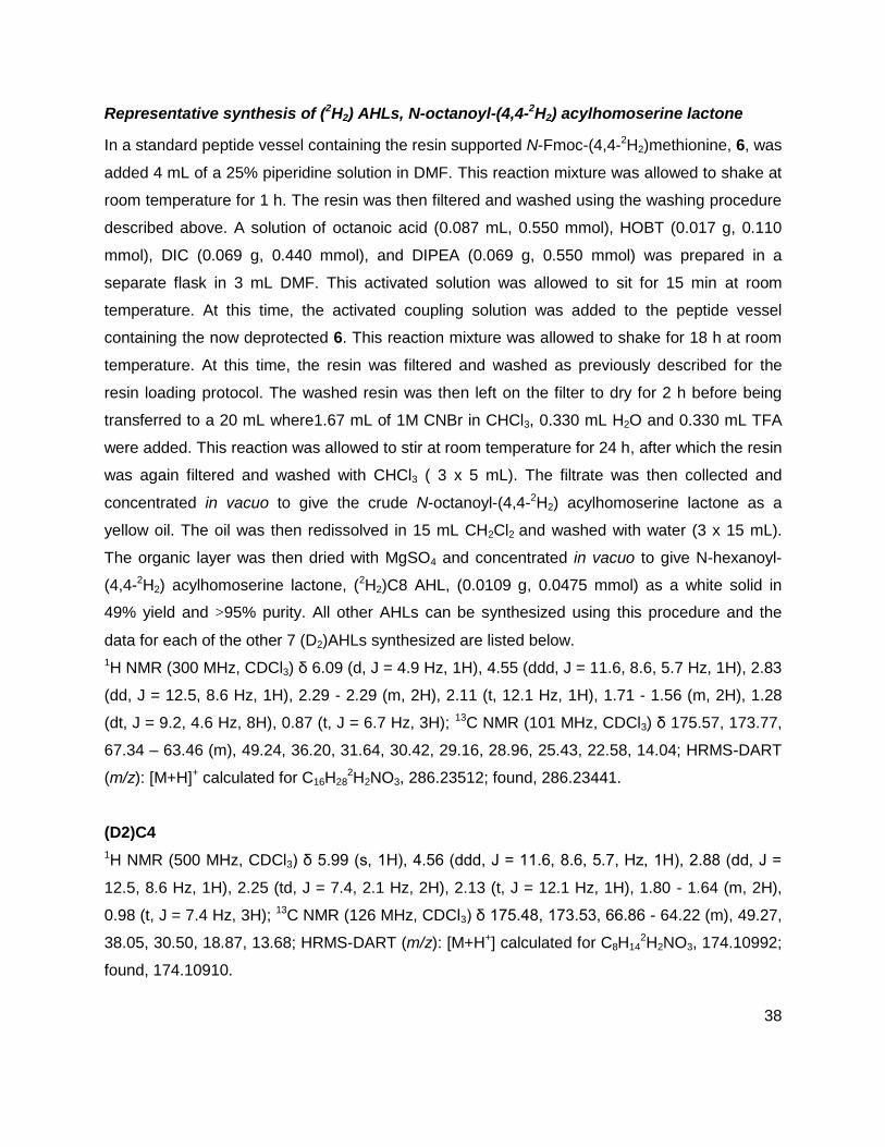
38

Representative synthesis of (2H2) AHLs, N-octanoyl-(4,4-2H2) acylhomoserine lactone

In a standard peptide vessel containing the resin supported N-Fmoc-(4,4-2H2)methionine, 6, was

added 4 mL of a 25% piperidine solution in DMF. This reaction mixture was allowed to shake at

room temperature for 1 h. The resin was then filtered and washed using the washing procedure

described above. A solution of octanoic acid (0.087 mL, 0.550 mmol), HOBT (0.017 g, 0.110

mmol), DIC (0.069 g, 0.440 mmol), and DIPEA (0.069 g, 0.550 mmol) was prepared in a

separate flask in 3 mL DMF. This activated solution was allowed to sit for 15 min at room

temperature. At this time, the activated coupling solution was added to the peptide vessel

containing the now deprotected 6. This reaction mixture was allowed to shake for 18 h at room

temperature. At this time, the resin was filtered and washed as previously described for the

resin loading protocol. The washed resin was then left on the filter to dry for 2 h before being

transferred to a 20 mL where1.67 mL of 1M CNBr in CHCl3, 0.330 mL H2O and 0.330 mL TFA

were added. This reaction was allowed to stir at room temperature for 24 h, after which the resin

was again filtered and washed with CHCl3 ( 3 x 5 mL). The filtrate was then collected and

concentrated in vacuo to give the crude N-octanoyl-(4,4-2H2) acylhomoserine lactone as a

yellow oil. The oil was then redissolved in 15 mL CH2Cl2 and washed with water (3 x 15 mL).

The organic layer was then dried with MgSO4 and concentrated in vacuo to give N-hexanoyl-

(4,4-2H2) acylhomoserine lactone, (2H2)C8 AHL, (0.0109 g, 0.0475 mmol) as a white solid in

49% yield and >95% purity. All other AHLs can be synthesized using this procedure and the

data for each of the other 7 (D2)AHLs synthesized are listed below.

1H NMR (300 MHz, CDCl3) δ 6.09 (d, J = 4.9 Hz, 1H), 4.55 (ddd, J = 11.6, 8.6, 5.7 Hz, 1H), 2.83

(dd, J = 12.5, 8.6 Hz, 1H), 2.29 - 2.29 (m, 2H), 2.11 (t, 12.1 Hz, 1H), 1.71 - 1.56 (m, 2H), 1.28

(dt, J = 9.2, 4.6 Hz, 8H), 0.87 (t, J = 6.7 Hz, 3H); 13C NMR (101 MHz, CDCl3) δ 175.57, 173.77,

67.34 – 63.46 (m), 49.24, 36.20, 31.64, 30.42, 29.16, 28.96, 25.43, 22.58, 14.04; HRMS-DART

(m/z): [M+H]+ calculated for C16H282H2NO3, 286.23512; found, 286.23441.

(D2)C4

1H NMR (500 MHz, CDCl3) δ 5.99 (s, 1H), 4.56 (ddd, J = 11.6, 8.6, 5.7, Hz, 1H), 2.88 (dd, J =

12.5, 8.6 Hz, 1H), 2.25 (td, J = 7.4, 2.1 Hz, 2H), 2.13 (t, J = 12.1 Hz, 1H), 1.80 - 1.64 (m, 2H),

0.98 (t, J = 7.4 Hz, 3H); 13C NMR (126 MHz, CDCl3) δ 175.48, 173.53, 66.86 - 64.22 (m), 49.27,

38.05, 30.50, 18.87, 13.68; HRMS-DART (m/z): [M+H+] calculated for C8H142H2NO3, 174.10992;

found, 174.10910.

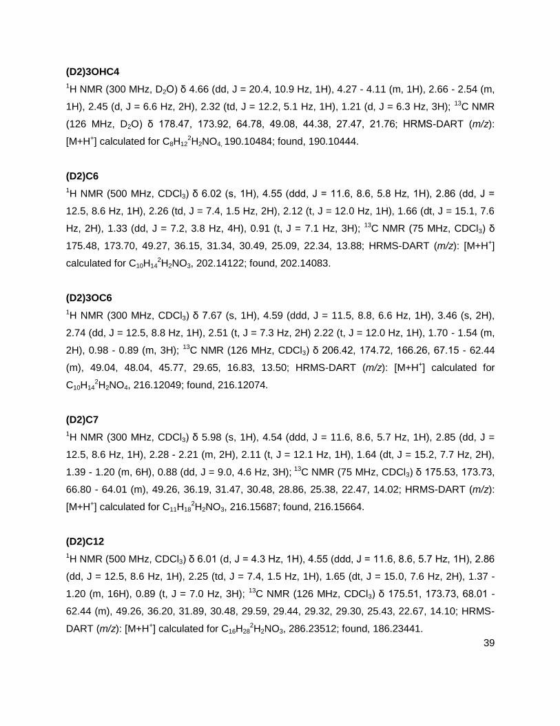
39

(D2)3OHC4

1H NMR (300 MHz, D2O) δ 4.66 (dd, J = 20.4, 10.9 Hz, 1H), 4.27 - 4.11 (m, 1H), 2.66 - 2.54 (m,

1H), 2.45 (d, J = 6.6 Hz, 2H), 2.32 (td, J = 12.2, 5.1 Hz, 1H), 1.21 (d, J = 6.3 Hz, 3H); 13C NMR

(126 MHz, D2O) δ 178.47, 173.92, 64.78, 49.08, 44.38, 27.47, 21.76; HRMS-DART (m/z):

[M+H+] calculated for C8H122H2NO4, 190.10484; found, 190.10444.

(D2)C6

1H NMR (500 MHz, CDCl3) δ 6.02 (s, 1H), 4.55 (ddd, J = 11.6, 8.6, 5.8 Hz, 1H), 2.86 (dd, J =

12.5, 8.6 Hz, 1H), 2.26 (td, J = 7.4, 1.5 Hz, 2H), 2.12 (t, J = 12.0 Hz, 1H), 1.66 (dt, J = 15.1, 7.6

Hz, 2H), 1.33 (dd, J = 7.2, 3.8 Hz, 4H), 0.91 (t, J = 7.1 Hz, 3H); 13C NMR (75 MHz, CDCl3) δ

175.48, 173.70, 49.27, 36.15, 31.34, 30.49, 25.09, 22.34, 13.88; HRMS-DART (m/z): [M+H+]

calculated for C10H142H2NO3, 202.14122; found, 202.14083.

(D2)3OC6

1H NMR (300 MHz, CDCl3) δ 7.67 (s, 1H), 4.59 (ddd, J = 11.5, 8.8, 6.6 Hz, 1H), 3.46 (s, 2H),

2.74 (dd, J = 12.5, 8.8 Hz, 1H), 2.51 (t, J = 7.3 Hz, 2H) 2.22 (t, J = 12.0 Hz, 1H), 1.70 - 1.54 (m,

2H), 0.98 - 0.89 (m, 3H); 13C NMR (126 MHz, CDCl3) δ 206.42, 174.72, 166.26, 67.15 - 62.44

(m), 49.04, 48.04, 45.77, 29.65, 16.83, 13.50; HRMS-DART (m/z): [M+H+] calculated for

C10H142H2NO4, 216.12049; found, 216.12074.

(D2)C7

1H NMR (300 MHz, CDCl3) δ 5.98 (s, 1H), 4.54 (ddd, J = 11.6, 8.6, 5.7 Hz, 1H), 2.85 (dd, J =

12.5, 8.6 Hz, 1H), 2.28 - 2.21 (m, 2H), 2.11 (t, J = 12.1 Hz, 1H), 1.64 (dt, J = 15.2, 7.7 Hz, 2H),

1.39 - 1.20 (m, 6H), 0.88 (dd, J = 9.0, 4.6 Hz, 3H); 13C NMR (75 MHz, CDCl3) δ 175.53, 173.73,

66.80 - 64.01 (m), 49.26, 36.19, 31.47, 30.48, 28.86, 25.38, 22.47, 14.02; HRMS-DART (m/z):

[M+H+] calculated for C11H182H2NO3, 216.15687; found, 216.15664.

(D2)C12


(dd, J = 12.5, 8.6 Hz, 1H), 2.25 (td, J = 7.4, 1.5 Hz, 1H), 1.65 (dt, J = 15.0, 7.6 Hz, 2H), 1.37 -

1.20 (m, 16H), 0.89 (t, J = 7.0 Hz, 3H); 13C NMR (126 MHz, CDCl3) δ 175.51, 173.73, 68.01 -

62.44 (m), 49.26, 36.20, 31.89, 30.48, 29.59, 29.44, 29.32, 29.30, 25.43, 22.67, 14.10; HRMS-

DART (m/z): [M+H+] calculated for C16H282H2NO3, 286.23512; found, 186.23441.

40

(D2)C14


(dd, J = 12.5, 8.6 Hz, 1H), 2.25 (td, J = 7.3, 1.4 Hz, 2H), 2.12 (t, J = 12.1 Hz, 1H), 1.65 (dt, 15.0,

7.6 Hz, 2H), 1.39 - 1.19 (M, 20H), 0.98 (t, J = 7.0 Hz, 3H); 13C NMR (126 MHz, CDCl3) δ 175.53,

173.74, 68.60 - 63.18 (m), 49.25, 36.20, 31.91, 30.45, 29.66, 29.63, 29.45, 29.31, 29.21, 25.43,

22.68, 14.11; HRMS-DART (m/z): [M+H+] calculated for C18H322H2NO3, 314.26642; found,

314.26532.

41

Chapter II

Determining Metabolic Profiles of Rat Insulinoma Cells

42

A version of this chapter was originally published by J. Jason Collier, Susan J. Burke, Mary E.

Eisenhauer, Danhong Lu, Renee C. Sapp, Carlie J. Frydman, and Shawn R. Campagna:

Collier JJ, Burke SJ, Eisenhauer ME, Lu D, Sapp RC, et al. (2011) Pancreatic β-Cell

Death in Response to Pro-Inflammatory Cytokines Is Distinct from Genuine Apoptosis. PLoS

ONE 6(7): e22485. doi:10.1371/journal.pone.0022485

The results and discussion, and methods and materials sections of the following chapter can be

found in the stated publication with no revisions as the author has been credited as a writer,

researcher, and analyzer for these sections. Results that were obtained by credited co-

researchers are clearly defined within the text.

Abstract

Type 1 Diabetes mellitus (T1DM) occurs in response to the autoimmune destruction of insulin

producing β-cells of the pancreas. It has been proposed that the method of β-cell death

proceeds by one of two mechanisms, necrosis or apoptosis, and that these mechanisms are

independent of each other and that one will prevail over the other preferentially. Until now,

T1DM has been studied mainly by genomic and proteomics techniques. While these techniques

are the standard in this field of research, a chemical approach, particularly at the level of

metabolism provides a better representation of what is happening in a system in real time. The

technological platform that addresses the metabolism of a given system is called metabolomics.

Often, metabolism will change in response to toxins or disease; the study of these systems in

response to a stimulus is one useful application of metabolomics. Here, a targeted

metabolomics mass spectrometry approach was employed to measure the metabolome of rat

islet β-cells that were exposed to inducers of cell death. This method was then used to

determine a metabolic profile for the two proposed mechanisms of β-cell death. Approximately

90 metabolites were observed that demonstrated statistically reliable and valid changes when

compared to a control group. In the profiles generated, several key differences were noted that

corresponded with supporting or previous findings. As a result, these findings provided evidence

that these stimuli not only resulted in a reduction in cell viability, but the metabolic profiles were

additionally distinct from one another.

43

Background and Significance

In the past 10 years, systems biology has grown in regards to technological platforms in which

systems can be explored and the data interpreted on the molecular level, with the emergence of

metabolomics being the newest of these platforms.55 The ability to accurately detect, identify

and quantitate the metabolites present in living organisms can provide a wealth of information

that complements other technologies such as genomics and proteomics in a variety of

biologically relevant applications.56-58 The analysis of molecular metabolism can be an effective

method to evaluate the state of a system. In the “omics” cascade, metabolism represents what

is actually happening in an organism after genes have been regulated, expressed as

phenotypes and finally modified post-transcriptionally. Further, it can be probed in systems

where stress of various forms has been applied. This chapter focuses on one of those

applications. T1DM is known to be caused by the reduction of insulin producing β-cells in the

Langerhans of the pancreas due to the death of these cells.59 Insulin deficiency then causes

increased blood glucose along with a multitude of symptoms that must be treated. Currently,

treatments of the disease usually include insulin injections, as there is no known cure for T1DM.

While it is known that β-cell death is a hallmark for T1DM, how these cells die, as well as why

they are specifically selected for destruction, remains largely unknown. Two mechanisms of cell

death have been proposed, although these have been debated. Conceivably, clarification as to

which mechanism, if either, is responsible for β-cell death will advance discussions of possible

treatments or cures for T1DM. Here, a mass spectrometry based metabolomics approach was

used to determine metabolic profiles for rat insulinoma cells treated with cell death inducers, in

an effort to explore mechanisms of cell death on a chemical level.

Metabolomics Background

Biologists rely on a number of analytical techniques to study the often complex systems of living

organisms. Starting at the genotypic level, there is what is described as the “omics” cascade

that consists of all the technology from which systems biology research is conducted. The

newest discipline to emerge is also closest to the phenotypic level and deals with the

metabolome.58 The metabolome refers to the set of all small molecule metabolites found in a

biological sample, and the technological platform has been termed metabolomics. Currently,

there is no single platform for the complete analysis of all the metabolites present in a single

44

system; however, over the past 10 years there have been an increasing number of papers

published that use metabolomics as a bioanalytical technique, demonstrating its usefulness as a

bioanalytical tool.60, 61 One possible reason that metabolomics has lagged behind other

techniques such as genomics and proteomics is that the metabolome is often dynamic and

complex. There are an estimated 2,000 major metabolites in mammalian organisms and up to

~200,000 in the plant kingdom, and these compounds represent a broad variety of chemical

classes with different chemical properties.60 Metabolite pools can change on the order of

seconds, and even slight environmental changes, such as a minor temperature change, can

result in changes in the metabolome. Despite the challenges associated with metabolomics, one

can easily recognize its benefits. Metabolism gives an accurate and timely view of the state of

the system and is often associated with the overall well-being of the organism or cell.

Metabolic Profiling vs. Metabolic Fingerprinting

The two major approaches to metabolomics include metabolic profiling and metabolic

fingerprinting. In most cases, metabolic profiling refers to the analysis of a certain group of

metabolites that is usually hypothesis driven and quantitative, also called a targeted analysis.

An example would be the analysis of fatty acids in a mammalian tissue. An even more specific

application is the selection of specific compounds for identification that may serve as biomarkers

of a disease or toxin exposure. This type of targeted analysis can be useful in supporting the

data collected from other technical “omics” platforms. Conversely, metabolic fingerprinting is the

global analysis of samples with the intent to obtain a characteristic metabolite pattern or

“fingerprint” and therefore, inherently an untargeted approach. This application is useful in

showing the overall change in metabolism in response to a treatment or alteration such as

genetic manipulations. Regardless of the sample or application, the steps leading to a

metabolomics data set are the same: sample collection, extraction, chemical analysis, and data

analysis.

Sample Type

Clinical applications of metabolomics have been useful in the field of human biology, where

fluids, such as serums and urine, can be quickly analyzed for changes in metabolic profiles in

response to disease, diet, toxins etc.62 This application, however, only provides information on

45

the metabolism of the organism as a whole, which usually provides no quantitative information,

and can also result in the introduction of additional variables. When dealing with individual cell

types, variables such as gender, environmental exposures, and contributions from different

tissues, essentially become non-existent due to the fact that the sample is often derived from a

controllable cell line as opposed to a human or animal model.60

Sampling and Extracting

The sampling in a metabolomics experiment should be determined by the experimental design

and type. In any case, the best results are obtained when the following are taken into

consideration: replication and quality control. Inter-day and multiple-day replications should be

taken in order to reduce biological variability. Additionally, the appropriate use of control

samples and/or internal standards can greatly enhance the statistical validity of the data set.

Once an experiment has been designed and the samples have been acquired, they must be

handled with extreme care as to not cause any disturbances in the existing metabolome. Often

this requires the use of cold temperatures to suspend metabolism. Some techniques used

include flash freezing, freeze clamping or immediate quenching. In cases where the

metabolome is not immediately extracted, the sample should be kept cold and the length of time

before extraction should be kept constant between all samples. The extraction technique will

vary with the experiment, but careful measures should be taken to ensure that all parameters of

a given experiment remain the same for all samples to be analyzed once an extraction

technique has been validated. Usually, the metabolome is extracted in order to separate the

metabolites from the complex biological matrices in which they are found, however direct

injection is one method of sample preparation. The extraction solvent should be suitable for the

type of sample. For example, a cold methanolic solution is usually used for mammalian tissue,

whereas more complex solvents, such as acidic acetonitrile mixtures, are typically used for

bacterial cultures.63 Here, the use of an internal standard spike can provide another means by

which the data set can be validated. It should be noted that in no experiment will the whole

metabolome remain intact. The very nature of the sample preparation step will guarantee that

some metabolites will be lost due to the fact that not all metabolites can be extracted by one

method.

46

Analytical Methods

After the sample has been collected and extracted, the final stages in a metabolomics

experiment are the analyses of the metabolites which include: separation, detection, and if

possible, quantification. Some of the requirements for obtaining scientifically relevant

metabolomics data are that the instruments used for analysis have excellent sensitivity and

resolution for a wide range of molecules, the ability to work with a variable range of metabolite

concentrations, relatively short analysis times, and reasonable reproducibility. Currently, the two

most widely used methods for metabolic analysis are nuclear magnetic resonance (NMR), and

mass spectrometry (MS). Both have their own particular advantages and disadvantages. With

NMR, samples require minimal preparation which preserves the sample.64, 65 NMR also offers

the ability to directly quantitate the relative abundance of metabolites in a sample, which can be

difficult to do with MS.

Mass Spectrometry Based Metabolomics

MS has come to the forefront of metabolomics research since becoming a successful tool in

drug metabolite analysis.61 The application of modern MS to cell culture metabolism is

particularly useful because of its high sensitivity and possibility for metabolite quantitation.

Several variations of MS have been implemented to study metabolism.61, 66, 67 One of the

simplest, direct injection has been useful for samples with sufficient metabolite content and

concentrations, such as urine. The major drawback of this method is that the biological matrix in

which the sample is located will usually reduce signal quality. Another problem associated with

direct injection is the difficulty when attempting to distinguish between analytes of the same

mass-to-charge ratio (m/z). When working with cell cultures, additional steps, such as the

incorporation of chromatography, are typically required for the analysis of global metabolism.

Variations such as gas chromatography mass spectrometry (GC-MS) and liquid

chromatography mass spectrometry (LC-MS) are often used in order to increase the number of

metabolites seen, however because of the complexity often involved with sample preparation in

GC-MS, LC-MS has taken a leading role in most MS metabolomics research.68 Considerations

when choosing a LC-MS method include 1) separation of the metabolites from the biological

matrix, 2) separation using chromatography, 3) analyte ionization, 4) detection of the fragment

and 5) identification. Again, separation of the metabolome from the matrix as well as using

chromatography is important for the overall signal quality. Reduction of the number of analytes

47

at a given time reduces the occurrence of ion suppression, and provides another level of

specificity. The ionization method most widely used for metabolomics has been electrospray

ionization (ESI). ESI is a soft ionization technique that ionizes liquid samples directly into the

gas phase, which is well suited for LC-MS. The number of metabolites measured increases

when both positive and negative ion modes are used. Metabolites such as amines will ionize

best in positive ion mode while acidic metabolites such as phosphates will ionize better in

negative mode. The two most common mass analyzers used in metabolomics directed research

are time-of-flight (TOF) and quadrupole analyzers.67 As mentioned in the previous chapter, the

preferred MS method used by our lab is detection by selected reaction monitoring (SRM) on a

triple quadrupole mass spectrometer. Coupled with separation by high performance liquid

chromatography (HPLC), this method has the sensitivity and selectivity required to detect up to

~350 polar metabolites as developed by Rabinowitz and co-workers. The target experiments

that will use this method will require that both the parent and product mass be known however,

a library of the ~350 metabolites was also created by Rabinowitz using chemical standards that

will be used in the studies presented in this chapter.

Data Analysis

The data sets generated by MS metabolomics techniques are often large and complex. The first

challenge encountered after data collection is the organization of these data into similar classes

by correctly identifying each individual metabolite.69 Often, the differences in metabolite pools

are of interest so it is imperative that metabolites are identified correctly. The use of chemical

standards and databases can greatly enhance identification, although these tools are still in the

beginning stages of development.70, 71 72 Software for the identification and selection of

chromatographic peaks has been important for evaluation of untargeted metabolomics data

sets.67 Once the metabolite has been identified, certain normalization factors will often be

applied to the raw data in order to correct for variability in the experiment. Once these have

been applied, the final task is to assemble the data for visualization.

Pancreatic β-cell Death

T1DM is an autoimmune disease that is characterized as the loss of the beta-cell mass of the

islets of the Langerhans in the pancreas that results in insulin deficiency.59 Pro-inflammatory

48

cytokines, such as interleukin-1β (IL-1β) and gamma-interferon (γ-IFN), induce the expression of

genes that produce inflammatory mediators, such as nitric oxide synthase (iNOS), and the

production and accumulation of nitric oxide (NO) inside the cell will inevitably decrease β-cell

viability.73, 74 While it is known that the secretion of pro-inflammatory cytokines play a role in β-

cell death, the initial cause and the precise method by which β-cells are destroyed are not fully

understood. Two mechanisms of cell death that are generally accepted, yet debated, are an

apoptotic pathway75, 76and/or a necrotic pathway.77, 78 Pro-inflammatory cytokines could induce

either of these pathways through a common bcl-2 inhibitory pathway, which makes discerning

the direct cause of β-cell death problematic.79 Apoptosis is a programmed form of cell death that

causes morphological changes in the cell which lead to irreversible damage.80 It is known to be

activated by a cascade of different caspases. With regards to β-cell death, initiation of the

apoptoside cascade results in targeted degradation of intracellular proteins that lead to cellular

death. When cleaved, one of these caspases, Caspase 3 (CASP3), is responsible for the

targeted destruction of intracellular proteins that lead to cell death.81 CASP3 activity is a known

marker for apoptosis mediated cell death. The pathways of non-apoptosis forms of cell death,

such as necrosis are even less understood.

There are several different models in which T1DM has been studied. The first animal model for

diabetes research was the non-obese diabetic (NOD) mouse model. Developed in 1970, this

strain sed develops the autoimmune disease spontaneously, similar to human T1DM.82 Even

with this model, the exact cellular mechanism behind β-cell death is unknown; the complexity of

the pathways involved in several different rat modeling systems has added confusion as to

which, if any of these pathways is actually involved in human T1DM.

Pancreatic β-cell Death is likely the Result of a Non-Apoptotic Mechanism

In a series of studies, pro- and anti-apoptotic proteins were subject to manipulation in order to

test the hypothesis that if apoptosis is indeed the primary pathway involved in β-cell death, then

exposure to cytokines known to be involved in a non-apoptotic method of cell death should be

protected the cell from damage.77 Several methods were implemented in order to first show that

apoptosis was not occurring in cells exposed to pro-inflammatory cytokines. First, the effects of

cytokines interleukin-1beta (IL-1β) and gamma-interferon (γ-IFN) were compared with the

effects of a known apoptosis inducer, camptothecin, in both a normal cytokine sensitive cell line

49

(832/13) and a cell line selected for cytokine resistance (833/15).83 Results indicated a 40%

decrease in viability in the 832/13 cell line when exposed to cytokines, and an identical 80%

decrease in viability in both cell lines with exposure to camptothecin This showed that selectivity

for cytokine resistance protected against death by exposure to the cytokines, but offered no

protection against exposure to apoptosis induced cell death. Next the 832/13 cell line was

subjected to overexpression of the anti-apoptotic protein kinase Akt1. This provided protection

against cell death when the cells were treated with camptothecin, but not with cytokines.

Additionally, siRNA mediated suppression of the proapoptotic protein Bax enhanced cell viability

in those treated with apoptosis inducers, but provided no protection in cells treated with

cytokines. In apoptosis, CASP3 activity can be measured via radioimmunoassay, and it was

verified that camptothecin induced CASP3 cleavage in both cell lines as well as isolated primary

cells. In contrast, NO is known to prevent caspase activity84; this was consistent with the finding

that no increase in CASP3 activity occurred in these cell lines treated with pro-inflammatory

cytokines. Another marker of apoptotic cell death, annexin V staining, was used, and results

again showed that camptothecin and not IL-1β and γ-IFN caused increases in staining. Finally,

intracellular ATP levels were examined. It has been suggested that ATP levels could be an

important biomarker for a switch from necrosis to apoptosis. Caspase activity requires energy,

and so it is presumed that intracellular ATP will be higher if apoptosis is occurring while ATP

levels will drop if a switch to a non-apoptosis pathway has occurred.85 Results in these studies

indeed showed that ATP levels increased in both sensitive and resistant cell lines treated with

camptothecin, while IL-1β and γ-IFN decreased ATP levels in the sensitive cell line 832/13 and

had no effect on the intracellular levels of ATP in the cytokine resistant cell line 833/15. Taken

together, these studies clearly support the idea that pro-inflammatory cytokine mediated β-cell

death proceeds by a mechanism independent and distinct from those known to occur in

apoptotic mediated pathways. It should be noted that previous reports with contradictory results

failed to employ a control for apoptosis such as a genuine apoptosis inducer.86, 87 Several

biomarkers are proven to be useful when attempting to distinguish between the two proposed

pathways. Therefore, we intended to study the metabolome of rat insulinoma cells which had

been exposed to either pro-inflammotory cytokines or known apoptosis inducers. If the

information obtained from the metabolome were consistent with the previous findings, then cell

lines treated with known apoptotic inducers should show differences in metabolites when

contrasted with cell lines treated with pro-inflammatory cytokines.

50

Results and Discussion

The unique intersection of the strategies previously employed by the Collier lab and mass

spectrometry based metabolomics developed by our lab aimed to further support the findings

that a non-apoptosis pathway is predominate in rat islet cells. The initial goal was to develop an

extraction method to analyze the metabolome of rat islet cells from two different cell lines. Given

that this type of analysis has never been initiated in any islet cell line, it was unknown as to

whether this method would ultimately provide any metabolic information. A preliminary

extraction was done using a typical mammalian tissue protocol63, and the supernatants

analyzed via liquid chromatography tandem mass spectrometry (LC-MS/MS) in SRM mode.

Results indicated the extraction performed and method of analysis was suitable for the islet

cells, so a series of studies was conducted on islet cells of various treatments. The treatments

used were specifically selected in order to compare the metabolic differences in islet cells where

apoptosis was induced versus cytokine exposure. This preliminary hypothesis presumes that

these two cellular mechanisms are independent and involve discretely separate metabolic

pathways, and therefore metabolic profiling of cells undergoing these two different mechanisms

of cell death will reveal differences in metabolite pools.

Distinction between Cell Death via Exposure to Pro-inflammatory Cytokines versus

Genuine Apoptosis Inducers

In a second series of studies conducted by the Collier lab, the hypothesis that pro-inflammatory

cytokines and apoptosis inducers differed in the mechanism by which cell death occurs was

further explored. In an effort to prove that the cytokine sensitive cell line 832/13 used in these

and past studies was just as sensitive to cytokine and apoptosis mediated killing as other cell

lines used in contradictory studies,88 an INS-1E derived cell line was first tested for viability

when exposed to both. It was found that both cell lines were equally sensitive to both inducers.

In order to further support the hypothesis that cytokine mediated cell death proceeds by a

different mechanism than apoptosis, key components from known pathways of each mechanism

were manipulated and tested for viability in response to both IL-1β and γ-IFN and camptothecin.

Manipulation of apoptosome by siRNA-mediated suppression of APAF-1 or a dominant-negative

form of capsase-9, protected against killing by camptothecin but not IL-1β and γ-IFN. Inhibition

of IKKβ, a known component of the NF-kB signaling pathway, by pharmacological inhibitor

51

TPCA or overexpression of an IκBα super repressor, blunted cytokine inducer NO production

and provided protection against losses in β-cell viability. No protection against camptothecin

mediated apoptosis was observed with either method.

Metabolic Profiling by Tandem Mass Spectrometry

From here, the metabolome of 832/13 rat islet cells treated separately with either

proinflammatory cytokines (IL-1β and γ-IFN), or an apoptosis inducer (camptothecin) was first

extracted, and then analyzed using the previously validated LC-MS/MS technique.89, 90 Again,

stemming from the previous findings, it was hypothesized that the metabolic profiling of the

differently treated cell lines would reveal differences in some metabolite pools and no

differences in others because the two different methods of β-cell death would be using different

metabolic pathways; cytokines induce cell death by increasing levels of intracellular NO into the

µM range, while apoptosis induces DNA damage through the caspase cascade. To show these

differences, fold changes in both treatments relative to a non-treated 832/13 cell sample were

considered. Figure 14 is a representative heatmap that displays these fold changes.

Approximately 130 metabolites were measured in positive mode and 175 were measured in

negative mode. Of these, 90 metabolites were verified to have changed with respect to the

control samples. Additionally, a table of p-values was constructed in order to determine the

probability that the differences seen in the treated cells relative to the non-treated cells were

indeed due to addition of the treatment (Tables 30 and 31, Appendix). In both cases, distinct

metabolic profiles were seen. However, it should be noted that although the concentration of

most metabolites in both the IL-1β and γ-IFN and camptothecin treated cells increase, this does

not necessarily indicate that these cells are more metabolically active than the control cells.

Metabolism changes can both be the result of a build-up of a metabolite or an increased use of

a metabolite, and it is impossible to distinguish between the causes of these changes in pool

size measurements, unless flux experiments are conducted. Regardless, obvious differences in

the metabolic response to the two different treatments were observed. One of the most notable

changes was the 400-fold increase in citrulline in cells treated with IL-1β and γ-IFN. Citrulline is

an end product of the iNOS reaction, and these results support the previous findings that NO

levels increase in cells treated with IL-1β and γ-IFN.

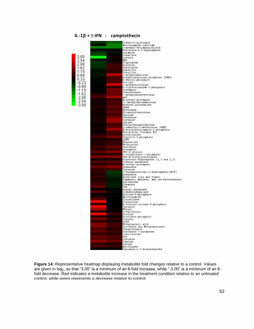
52

IL -1β + γ-IFN : camptothecin

Figure 14: Representative heatmap displaying metabolite fold changes relative to a control. Values are given in log2, so that “3.00” is a minimum of an 8-fold increase, while “-3.00” is a minimum of an 8-fold decrease. Red indicates a metabolite increase in the treatment condition relative to an untreated control, while green represents a decrease relative to control.

53

Methods and Materials

General Methods

The LC-MS/MS system used for detection of metabolites consisted of a Thermo Electron

Surveyor Autosampler Plus, a Surveyor MS Pump Plus, and a TSQ Quantum Discovery Max

triple quadrupole MS. All MS spectra were collected and analyzed using the Xcalibur MS v 2.0.7

software package (Thermo Electron Corporation). HPLC separations performed in positive

mode used a Luna NH2 HILIC column (5µm pore size, 100 Å particle size, 250 x 2.00 mm)

supplied by Phenomenex. HPLC separations performed in negative mode used a Synergi

Hydro-RP C18 column (4 µm pore size, 80 Å particle size, 150 x 2.00 mm) supplied by

Phenomenex.

Cell Extraction Procedure

832/13 cells were grown to confluence in 15 cm dishes and treated as indicated in the figure

legends. At the end of the treatment period, cells were washed twice with ice cold phosphate

buffered saline, scraped and pelleted at 500 x g; the aspirated dry cell pellets were immediately

flash frozen using liquid N2. Four individual experiments were performed in duplicate on each of

3 days. Prior to extraction, the collected cell pellets were weighed, and 30-50 mg of each was

placed into a microcentrifuge tube at -78 °C. A solution of cold methanol and water (8:2 v/v, 1.5

mL) kept at -80 °C was then added to the tube to extract the metabolome from the cells. The

contents were mixed by vortexing and allowed to sit at the extraction temperature for 20 min.

Particulates were then removed from the samples by centrifugation, and the supernatants were

transferred to autosampler vials for further analysis by the LC-MS/MS methods described

below.

Chromatographic Details

High performance liquid chromatographic separations of metabolites were performed via a slight

modification of previously reported methods.91 Due to slight changes, methods are also

reported below. In total, two HPLC runs are necessary to fully characterize the metabolome for

each sample since separate detection for positively ionizing and negatively ionizing compounds

is required. For all samples, 10 µL was injected onto the column via an autosampler. A

54

quaternary pump was used to generate the following gradient for the elution of compounds from

the stationary phase:

Positive Mode

The mobile phase flow rate was150 µL/min, and a gradient of two solvents was used for elution.

Solvent A was a mixture composed of 95% 20 mM ammonium acetate and 20 mM ammonium

hydroxide in HPLC grade water buffered at pH = 9.4 with 5% HPLC grade acetonitrile. Solvent

B was pure HPLC grade acetonitrile. These were used to construct the following 40 min

gradient elution profile: t = 0 min, 15% solvent A, 85% solvent B; t = 15 min, 100% solvent A,

0% solvent B; t = 28 min, 100% solvent A, 0% solvent B; t = 30, 15% solvent A, 85% solvent B; t

= 40, 15% solvent A, 85% solvent B. Separations were performed with the column temperature

set at 10 oC.

Negative Mode

The mobile phase flow rate was 200 µL/min, and a gradient of two solvents was again used for

elution. Solvent A consisted of a mixture containing 97% 11 mM tributylamine and 15 mM

acetic acid in HPLC grade water and 3% HPLC grade methanol. Solvent B was pure HPLC

grade methanol. These were used to construct the following 50 min gradient elution profile: t = 0

min, 100% solvent A, 0% solvent B; t = 5 min, 100% solvent A, 0% solvent B; t = 10 min, 80%

solvent A, 20% solvent B; t = 15, 80% solvent A, 20% solvent B; t = 30, 35% solvent A, 65%

solvent B; t = 33, 5% solvent A, 95% solvent B; t = 37, 5% solvent A, 95% solvent B; t = 38,

100% solvent A, 0% solvent B; t = 50, 100% solvent A, 0% solvent B. Separations were

performed with the column temperature maintained at 25 oC.

Mass Spectrometric Detection Parameters

Samples were introduced into the electrospray ionization (ESI) chamber through a 0.1 mm

internal diameter fused silica capillary after delivery by HPLC as described above. The spray

voltage for the ESI source was set to 4500 V, if detection occurred in positive ion mode. If

detection occurred in negative mode, the spray voltage for the ESI source was set to 3000 V.

Nitrogen was used as the sheath gas (40 psi), and the inlet capillary temperature was 290 °C.

Argon was used as the collision gas at a pressure of 1.5 mTorr. Samples were analyzed using

selected reaction monitoring (SRM) with the scan time for each SRM set to 0.05 s and a scan

55

width of 1 m/z. Full selected reaction monitoring (SRM) detection parameters for most

compounds have been previously reported by Rabinowitz and coworkers.91

Data Handling and Statistical Anaylsis

The peak for each detected metabolite was manually integrated to determine the peak area

using the Quan Browser function of Xcalibur. The integration values were then directly entered

into an Excel spreadsheet where they were normalized to the mass of tissue extracted. Since

inter-day variability in the ion counts for metabolites was observed due to MS sampling

variation, the treated samples were compared only to the control samples run on the same day.

This comparison consisted of averaging the ion counts for the duplicate measurements of a

metabolite from a treated sample on a given day and then dividing this number by the average

of the duplicate measurements of the same metabolite from the control sample obtained on the

same day to generate the fold change for the compound. The fold changes for the metabolite

from each of the three days were then averaged and clustered and displayed in heat map

format using the freely available Cluster 3.0 (www.falw.vu/~huik/cluster.htm) and Java

Treeview92 data analysis packages. The p-value for each metabolite fold change was obtained

by performing an F-test using the data analysis tool pack in Microsoft Excel. The variance in the

fold changes for the metabolites in the treatment group was compared to a set of standardized

fold changes for the metabolites from the control group that was generated by taking the intra-

day ratio of the ion counts from the duplicate measurements of the control.

56

Conclusion

The tools available to a chemist or biologist can greatly impact the scope and quality of research

conducted. Here, a chemical approach conducted with analytical techniques was applied to the

study of two biological systems. Quantitation of both systems, absolute for quorum sensing

molecules, and relative for the metabolic profiling of rat insulinoma cells, were ultimately

achieved using LC-MS/MS methods, providing novel results as well as further questions.

The synthesis of stable isotopically labeled AHLs allowed for the quantitation of the naturally

occurring molecules in four strains of Vibrio fischeri. This synthesis proved to be exceptionally

valuable for AHL studies in any bacterial system, as it was able to produce any AHL necessary

with minimal purification. Additionally, the AI-2 mediated quorum sensing systems of Yersinia

enterocolitica and Edwardsiella tarda were analyzed. Results from these studies contribute to

the growing amount of information about quorum sensing systems, and have been useful in

efforts to better understand these systems.

The application of known LC-MS/MS methods to the study of rat insulinoma cells provided

visibly distinctive metabolic profiles for two proposed mechanisms of β-cell death. Taken

together with results from the Collier lab, we were able to conclude that β-cell death in response

to pro-inflammatory cytokines is unlikely to proceed through an apoptotic mechanism. Further

studies are currently underway to continue probing these mechanisms metabolically, with the

ultimate goal of determining the exact cause of pancreatic β-cell death and eventually, T1DM.

57

References

58

1. Fuqua, C., Parsek, M. R., and Greenberg, E. P. (2001) Regulation of gene expression by cell-to-cell communication: Acyl-homoserine lactone quorum sensing, Annual Review of Genetics 35, 439-468.

2. Miller, M. B., and Bassler, B. L. (2001) Quorum sensing in bacteria, Annual Review of Microbiology 55, 165-199.

3. Waters, C. M. (2005) Quorum sensing: Cell-to-cell communication in bacteria, In Annual Review of Cell and Developmental Biology, pp 319-346.

4. Fuqua, W. C., Winans, S. C., and Greenberg, E. P. (1994) Quorum Sensing in Bacteria - The LuxR-LuxI Family of Density-Responsive Transcriptional Regulators, Journal of Bacteriology 176, 269-275.

5. Hall-Stoodley, L., Costerton, J. W., and Stoodley, P. (2004) Bacterial biofilms: From the natural environment to infectious diseases, Nature Reviews Microbiology 2, 95-108.

6. Dickschat, J. S. (2010) Quorum sensing and bacterial biofilms, Natural Product Reports 27, 343-369.

7. Donlan, R. M. (2002) Biofilms: Microbial life on surfaces, Emerging Infectious Diseases 8, 881-890.

8. Rickard, A. H., Colacino, K. R., Manton, K. M., Morton, R. I., Pulcini, E., Pfeil, J., Rhoads, D., Wolcott, R. D., and James, G. (2010) Production of cell-cell signalling molecules by bacteria isolated from human chronic wounds, Journal of Applied Microbiology 108, 1509-1522.

9. Singh, P. K., Schaefer, A. L., Parsek, M. R., Moninger, T. O., Welsh, M. J., and Greenberg, E. P. (2000) Quorum-sensing signals indicate that cystic fibrosis lungs are infected with bacterial biofilms, Nature 407, 762-764.

10. Lyczak, J. B., Cannon, C. L., and Pier, G. B. (2002) Lung infections associated with cystic fibrosis, Clinical Microbiology Reviews 15, 194.

11. Bjarnsholt, T., and Givskov, M. (2007) Quorum-sensing blockade as a strategy for enhancing host defences against bacterial pathogens, Philosophical Transactions of the Royal Society B-Biological Sciences 362, 1213-1222.

12. Kaufmann, G. F., Park, J., and Janda, K. D. (2008) Bacterial quorum sensing: a new target for anti-infective immunotherapy, Expert Opinion on Biological Therapy 8, 719-724.

13. Boyer, M., and Wisniewski-Dye, F. (2009) Cell-cell signalling in bacteria: not simply a matter of quorum, Fems Microbiology Ecology 70, 1-19.

14. Platt, T. G., and Fuqua, C. (2010) What's in a name? The semantics of quorum sensing, Trends in Microbiology 18, 383-387.

15. Xavier, K. B., and Bassler, B. L. (2003) LuxS quorum sensing: more than just a numbers game, Current Opinion in Microbiology 6, 191-197.

16. Bassler, B. L. (1999) How bacteria talk to each other: regulation of gene expression by quorum sensing, Current Opinion in Microbiology 2, 582-587.

59

17. Lupp, C., Urbanowski, M., Greenberg, E. P., and Ruby, E. G. (2003) The Vibrio fischeri quorum-sensing systems ain and lux sequentially induce luminescence gene expression and are important for persistence in the squid host, Molecular Microbiology 50, 319-331.

18. Passador, L., Cook, J. M., Gambello, M. J., Rust, L., and Iglewski, B. H. (1993) Expression of Pseudomonas aeruginosa virulence genes requires cel-to-cell communication, Science 260, 1127-1130.

19. Jaques, S., and Mccarter, L. L. (2006) Three new regulators of swarming in Vibrio parahaemolyticus, Journal of Bacteriology 188, 2625-2635.

20. Kleerebezem, M., Quadri, L. E. N., Kuipers, O. P., and Devos, W. M. (1997) Quorum sensing by peptide pheromones and two-component signal-transduction systems in Gram-positive bacteria, Molecular Microbiology 24, 895-904.

21. Surette, M. G., Miller, M. B., and Bassler, B. L. (1999) Quorum sensing in Escherichia coli, Salmonella typhimurium, and Vibrio harveyi: A new family of genes responsible for autoinducer production, Proceedings of the National Academy of Sciences of the United States of America 96, 1639-1644.

22. Bassler, B. L., Wright, M., Showalter, R. E., and Silverman, M. R. (1993) Intercellular Signaling in Vibrio harveyi - sequence and Function of Genes Regulating Expression of Luminescence, Molecular Microbiology 9, 773-786.

23. Chen, X., Schauder, S., Potier, N., Van Dorsselaer, A., Pelczer, I., Bassler, B. L., and Hughson, F. M. (2002) Structural identification of a bacterial quorum-sensing signal containing boron, Nature 415, 545-549.

24. Schauder, S., Shokat, K., Surette, M. G., and Bassler, B. L. (2001) The LuxS family of bacterial autoinducers: biosynthesis of a novel quorum-sensing signal molecule, Molecular Microbiology 41, 463-476.

25. Miller, C. H., and Duerre, J. A. (1968) S-ribosylhomocysteinase cleavage enzyme from Escherichia coli, Journal of Biological Chemistry 243, 92-&.

26. Visick, K. L., Foster, J., Doino, J., Mcfall-Ngai, M., and Ruby, E. G. (2000) Vibrio fischeri lux genes play an important role in colonization and development of the host light organ, Journal of Bacteriology 182, 4578-4586.

27. Whitehead, N. A., Barnard, A. M. L., Slater, H., Simpson, N. J. L., and Salmond, G. P. C. (2001) Quorum-sensing in gram-negative bacteria, Fems Microbiology Reviews 25, 365-404.

28. Fuqua, C., and Greenberg, E. P. (2002) Listening in on bacteria: Acyl-homoserine lactone signalling, Nature Reviews Molecular Cell Biology 3, 685-695.

29. Fuqua, C., Winans, S. C., and Greenberg, E. P. (1996) Census and consensus in bacterial ecosystems: The LuxR-LuxI family of quorum-sensing transcriptional regulators, Annual Review of Microbiology 50, 727-751.

30. Halliday, N. M., Hardie, K. R., Williams, P., Winzer, K., and Barrett, D. A. (2010) Quantitative liquid chromatography-tandem mass spectrometry profiling of activated methyl cycle metabolites involved in LuxS-dependent quorum sensing in Escherichia coli, Analytical Biochemistry 403, 20-29.

60

31. Waters, C. M., and Bassler, B. L. (2006) The Vibrio harveyi quorum-sensing system uses shared regulatory components to discriminate between multiple autoinducers, Genes & Development 20, 2754-2767.

32. Xavier, K. B., and Bassler, B. L. (2005) Regulation of uptake and processing of the quorum-sensing autoinducer AI-2 in Escherichia coli, Journal of Bacteriology 187, 238-248.

33. Gooding, J. R., May, A. L., Hilliard, K. R., and Campagna, S. R. (2010) Establishing a Quantitative Definition of Quorum Sensing Provides Insight into the Information Content of the Autoinducer Signals in Vibrio harveyi and Escherichia coli, Biochemistry 49, 5621-5623.

34. Piper, K. R., Vonbodman, S. B., and Farrand, S. K. (1993) Conjugation factor of Agrobacterium tumefaciens regulates TI-plasmid transfer by autoinduction, Nature 362, 448-450.

35. Shaw, P. D., Ping, G., Daly, S. L., Cha, C., Cronan, J. E., Rinehart, K. L., and Farrand, S. K. (1997) Detecting and characterizing N-acyl-homoserine lactone signal molecules by thin-layer chromatography, Proceedings of the National Academy of Sciences of the United States of America 94, 6036-6041.

36. Blosser-Middleton, R. S., and Gray, K. M. (2001) Multiple N-acyl homoserine lactone signals of Rhizobium leguminosarum are synthesized in a distinct temporal pattern, Journal of Bacteriology 183, 6771-6777.

37. Charlton, T. S., De Nys, R., Netting, A., Kumar, N., Hentzer, M., Givskov, M., and Kjelleberg, S. (2000) A novel and sensitive method for the quantification of N-3-oxoacyl homoserine lactones using gas chromatography-mass spectrometry: application ito a model bacterial biofilm, Environmental Microbiology 2, 530-541.

38. Thiel, V., Kunze, B., Verma, P., Wagner-Dobler, I., and Schulz, S. (2009) New Structural Variants of Homoserine Lactones in Bacteria, Chembiochem 10, 1861-1868.

39. Morin, D., Grasland, B., Vallee-Rehel, K., Dufau, C., and Haras, D. (2003) On-line high-performance liquid chromatography-mass spectrometric detection and quantification of N-acylhomoserine lactones, quorum sensing signal molecules, in the presence of biological matrices, Journal of Chromatography A 1002, 79-92.

40. Ortori, C. A., Atkinson, S., Chhabra, S. R., Camara, M., Williams, P., and Barrett, D. A. (2007) Comprehensive profiling of N-acylhomoserine lactones produced by Yersinia pseudotuberculosis using liquid chromatography coupled to hybrid quadrupole-linear ion trap mass spectrometry, Analytical and Bioanalytical Chemistry 387, 497-511.

41. Campagna, S. R., Gooding, J. R., and May, A. L. (2009) Direct Quantitation of the Quorum Sensing Signal, Autoinducer-2, in Clinically Relevant Samples by Liquid Chromatography-Tandem Mass Spectrometry, Analytical Chemistry 81, 6374-6381.

42. Semmelhack, M. F., Campagna, S. R., Federle, M. J., and Bassler, B. L. (2005) An expeditious synthesis of DPD and boron binding studies, Organic Letters 7, 569-572.

43. Gould, T. A., Herman, J., Krank, J., Murphy, R. C., and Churchill, M. E. A. (2006) Specificity of acyl-homoserine lactone synthases examined by mass spectrometry, Journal of Bacteriology 188, 773-783.

61

44. Kai, K., Tani, A., and Hayashi, H. (2010) Facile preparation of deuterium-labeled N-acylhomoserine lactones as internal standards for isotope dilution mass spectrometry, Bioorganic & Medicinal Chemistry 18, 3776-3782.

45. Yang, C. C., and Merrifield, R. B. (1976) Beta-phenacyl ester as a temporary protecting group to minimize cyclic imide formation during subsequent treatment of aspartyl peptides with HF, Journal of Organic Chemistry 41, 1032-1041.

46. Ramalingam, K., and Woodard, R. W. (1988) Synthesis of Stereospecific Deuterium-Labeled Homoserines and Homoserine Lactones, Journal of Organic Chemistry 53, 1900-1903.

47. Kumari, A., Pasini, P., and Daunert, S. (2008) Detection of bacterial quorum sensing N-acyl homoserine lactones in clinical samples, Analytical and Bioanalytical Chemistry 391, 1619-1627.

48. Ortori, C. A., Dubern, J.-F., Chhabra, S. R., Camara, M., Hardie, K., Williams, P., and Barrett, D. A. (2011) Simultaneous quantitative profiling of N-acyl-l-homoserine lactone and 2-alkyl-4(1H)-quinolone families of quorum-sensing signaling molecules using LC-MS/MS, Analytical and Bioanalytical Chemistry 399, 839-850.

49. Wang, F., Zhang, M., Hu, Y. H., Zhang, W. W., and Sun, L. (2009) Regulation of the Edwardsiella tarda Hemolysin Gene and LuxS by EthR, Journal of Microbiology and Biotechnology 19, 765-773.

50. Zhang, M., Jiao, X. D., Hu, Y. H., and Sun, L. (2009) Attenuation of Edwardsiella tarda Virulence by Small Peptides That Interfere with LuxS/Autoinducer Type 2 Quorum Sensing, Applied and Environmental Microbiology 75, 3882-3890.

51. Heermann, R., and Fuchs, T. M. (2008) Comparative analysis of the Photorhabdus luminescens and the Yersinia enterocolitica genomes: uncovering candidate genes involved in insect pathogenicity, Bmc Genomics 9.

52. Sezonov, G., Joseleau-Petit, D., and D'ari, R. (2007) Escherichia coli physiology in Luria-Bertani broth, Journal of Bacteriology 189, 8746-8749.

53. Dalsgaard, I. (2001) Selection of media for antimicrobial susceptibility testing of fish pathogenic bacteria, Aquaculture 196, 267-275.

54. Lloyd, J. B., and Whelan, W. J. (1969) An Improved Method for Enzymatic Determination of Glucose in Presence of Maltose, Analytical Biochemistry 30, 467.

55. Weckwerth, W. (2003) Metabolomics in systems biology, Annual Review of Plant Biology 54, 669-689.

56. Bino, R. J., Hall, R. D., Fiehn, O., Kopka, J., Saito, K., Draper, J., Nikolau, B. J., Mendes, P., Roessner-Tunali, U., Beale, M. H., Trethewey, R. N., Lange, B. M., Wurtele, E. S., and Sumner, L. W. (2004) Potential of metabolomics as a functional genomics tool, Trends in Plant Science 9, 418-425.

57. Fiehn, O. (2001) Combining genomics, metabolome analysis, and biochemical modelling to understand metabolic networks, Comparative and Functional Genomics 2, 155-168.

58. Fiehn, O. (2002) Metabolomics - the link between genotypes and phenotypes, Plant Molecular Biology 48, 155-171.

62

59. Mathis, D., Vence, L., and Benoist, C. (2001) Beta-cell death during progression to diabetes, Nature 414, 792-798.

60. Cuperlovic-Culf, M., Barnett, D. A., Culf, A. S., and Chute, I. (2010) Cell culture metabolomics: applications and future directions, Drug Discovery Today 15, 610-621.

61. Dettmer, K., Aronov, P. A., and Hammock, B. D. (2007) Mass spectrometry-based metabolomics, Mass Spectrometry Reviews 26, 51-78.

62. Hirai, M. Y., Yano, M., Goodenowe, D. B., Kanaya, S., Kimura, T., Awazuhara, M., Arita, M., Fujiwara, T., and Saito, K. (2004) Integration of transcriptomics and metabolomics for understanding of global responses to nutritional stresses in Arabidopsis thaliana, Proceedings of the National Academy of Sciences of the United States of America 101, 10205-10210.

63. Yuan, J., Bennett, B. D., and Rabinowitz, J. D. (2008) Kinetic flux profiling for quantitation of cellular metabolic fluxes, Nature Protocols 3, 1328-1340.

64. Dunn, W. B., and Ellis, D. I. (2005) Metabolomics: Current analytical platforms and methodologies, Trac-Trends in Analytical Chemistry 24, 285-294.

65. Viant, M. R., Rosenblum, E. S., and Tjeerdema, R. S. (2003) NMR-based metabolomics: A powerful approach for characterizing the effects of environmental stressors on organism health, Environmental Science & Technology 37, 4982-4989.

66. Dunn, W. B., Bailey, N. J. C., and Johnson, H. E. (2005) Measuring the metabolome: current analytical technologies, Analyst 130, 606-625.

67. Want, E. J., Nordstrom, A., Morita, H., and Siuzdak, G. (2007) From exogenous to endogenous: The inevitable imprint of mass spectrometry in metabolomics, Journal of Proteome Research 6, 459-468.

68. Wilson, I. D., Plumb, R., Granger, J., Major, H., Williams, R., and Lenz, E. A. (2005) HPLC-MS-based methods for the study of metabonomics, Journal of Chromatography B-Analytical Technologies in the Biomedical and Life Sciences 817, 67-76.

69. Kell, D. B. (2004) Metabolomics and systems biology: making sense of the soup, Current Opinion in Microbiology 7, 296-307.

70. Katajamaa, M., and Oresic, M. (2005) Processing methods for differential analysis of LC/MS profile data, Bmc Bioinformatics 6.

71. Wishart, D. S., Tzur, D., Knox, C., Eisner, R., Guo, A. C., Young, N., Cheng, D., Jewell, K., Arndt, D., Sawhney, S., Fung, C., Nikolai, L., Lewis, M., Coutouly, M. A., Forsythe, I., Tang, P., Shrivastava, S., Jeroncic, K., Stothard, P., Amegbey, G., Block, D., Hau, D. D., Wagner, J., Miniaci, J., Clements, M., Gebremedhin, M., Guo, N., Zhang, Y., Duggan, G. E., Macinnis, G. D., Weljie, A. M., Dowlatabadi, R., Bamforth, F., Clive, D., Greiner, R., Li, L., Marrie, T., Sykes, B. D., Vogel, H. J., and Querengesser, L. (2007) HMDB: the human metabolome database, Nucleic Acids Research 35, D521-D526.

72. Schauer, N., Steinhauser, D., Strelkov, S., Schomburg, D., Allison, G., Moritz, T., Lundgren, K., Roessner-Tunali, U., Forbes, M. G., Willmitzer, L., Fernie, A. R., and Kopka, J. (2005) GC-MS libraries for the rapid identification of metabolites in complex biological samples, Febs Letters 579, 1332-1337.

63

73. Corbett, J. A., and Mcdaniel, M. L. (1992) Does Nitric Oxide Mediate Autoimmune Destruction of Beta-Cells - Possible Therapeutic Interventions in IDDM, Diabetes 41, 897-903.

74. Mandruppoulsen, T., Spinas, G. A., Prowse, S. J., Hansen, B. S., Jorgensen, D. W., Bendtzen, K., Nielsen, J. H., and Nerup, J. (1987) Islet cytotoxicity of interleukin-1 - Influence of culture conditions and islet donor characteristics, Diabetes 36, 641-647.

75. Grunnet, L. G., Aikin, R., Tonnesen, M. F., Paraskevas, S., Blaabjerg, L., Storling, J., Rosenberg, L., Billestrup, N., Maysinger, D., and Mandrup-Poulsen, T. (2009) Proinflammatory Cytokines Activate the Intrinsic Apoptotic Pathway in beta-Cells, Diabetes 58, 1807-1815.

76. Gurzov, E. N., Germano, C. M., Cunha, D. A., Ortis, F., Vanderwinden, J.-M., Marchetti, P., Zhang, L., and Eizirik, D. L. (2010) p53 Up-regulated Modulator of Apoptosis (PUMA) Activation Contributes to Pancreatic beta-Cell Apoptosis Induced by Proinflammatory Cytokines and Endoplasmic Reticulum Stress, Journal of Biological Chemistry 285, 19910-19920.

77. Collier, J. J., Fueger, P. T., Hohmeier, H. E., and Newgard, C. B. (2006) Pro- and antiapoptotic proteins regulate apoptosis but do not protect against cytokine-mediated cytotoxicity in rat islets and beta-cell lines, Diabetes 55, 1398-1406.

78. Fehsel, K., Kolb-Bachofen, V., and Kroncke, K. D. (2003) Necrosis is the predominant type of islet cell death during development of insulin-dependent diabetes mellitus in BB rats, Laboratory Investigation 83, 549-559.

79. Saldeen, J. (2000) Cytokines induce both necrosis and apoptosis via a common bcl-2-inhibitable pathway in rat insulin-producing cells, Endocrinology 141, 2003-2010.

80. Kerr, J. F. R., Wyllie, A. H., and Currie, A. R. (1972) Apoptosis - Basic Biological Phenomenon with Wide-Ranging Implications in Tissue Kinetics, British Journal of Cancer 26, 239.

81. Taylor, R. C., Cullen, S. P., and Martin, S. J. (2008) Apoptosis: controlled demolition at the cellular level, Nature Reviews Molecular Cell Biology 9, 231-241.

82. Reddy, S., Bradley, J., and Ross, J. M. (2003) Immunolocalization of caspase-3 in pancreatic islets of NOD mice during cyclophosphamide-accelerated diabetes, In Immunology of Diabetes Ii: Pathogenesis from Mouse to Man (Sanjeevi, C. B., and Eisenbarth, G. S., Eds.), pp 192-195.

83. Chen, G. X., Hohmeier, H. E., Gasa, R., Tran, V. V., and Newgard, C. B. (2000) Selection of insulinoma cell lines with resistance to interleukin-1 beta- and gamma-interferon-induced cytotoxicity, Diabetes 49, 562-570.

84. Zech, B., Kohl, R., Von Knethen, A., and Brune, B. (2003) Nitric oxide donors inhibit formation of the Apaf-1/caspase-9 apoptosome and activation of caspases, Biochemical Journal 371, 1055-1064.

85. Nicotera, P., and Merlino, G. (2004) Regulation of the apoptosis-necrosis switch, Oncogene 23, 2757-2765.

86. Li, L., El-Kholy, W., Rhodes, C. J., and Brubaker, P. L. (2005) Glucagon-like peptide-1 protects beta cells from cytokine-induced apoptosis and necrosis: role of protein kinase B, Diabetologia 48, 1339-1349.

64

87. Rakatzi, I., Mueller, H., Ritzeler, O., Tennagels, N., and Eckel, J. (2004) Adiponectin counteracts cytokine- and fatty acid-induced apoptosis in the pancreatic beta-cell line INS-1, Diabetologia 47, 249-258.

88. Heitmeier, M. R., Scarim, A. L., and Corbett, J. A. (1999) Prolonged STAT1 activation is associated with interferon-gamma priming for interleukin-1-induced inducible nitric-oxide synthase expression by islets of Langerhans, Journal of Biological Chemistry 274, 29266-29273.

89. Waters, C. A., Lu, W., Rabinowitz, J. D., and Bassler, B. L. (2008) Quorum sensing controls biofilm formation in Vibrio cholerae through modulation of cyclic Di-GMT levels and repression of vpsT, Journal of Bacteriology 190, 2527-2536.

90. Lu, W., Bennett, B. D., and Rabinowitz, J. D. (2008) Analytical strategies for LC-MS-based targeted metabolomics, Journal of Chromatography B-Analytical Technologies in the Biomedical and Life Sciences 871, 236-242.

91. Bajad, S. U., Lu, W., Kimball, E. H., Yuan, J., Peterson, C., and Rabinowitz, J. D. (2006) Separation and quantitation of water soluble cellular metabolites by hydrophilic interaction chromatography-tandem mass spectrometry, Journal of Chromatography A 1125, 76-88.

92. Saldanha, A. J. (2004) Java Treeview-extensible visualization of microarray data, Bioinformatics 20, 3246-3248.

65

Appendix

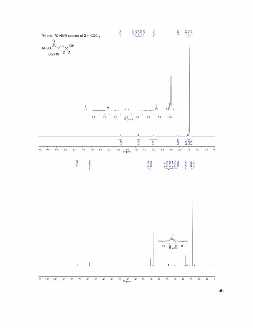
66

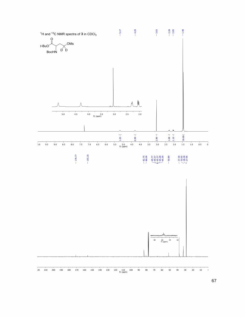
67

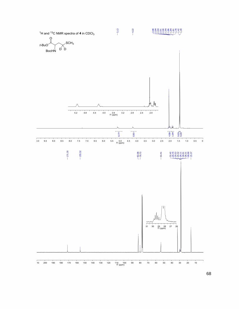
68

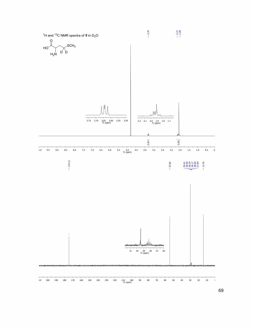
69

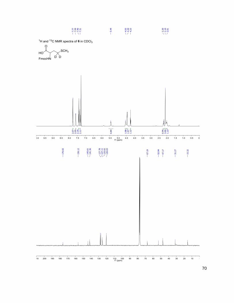
70

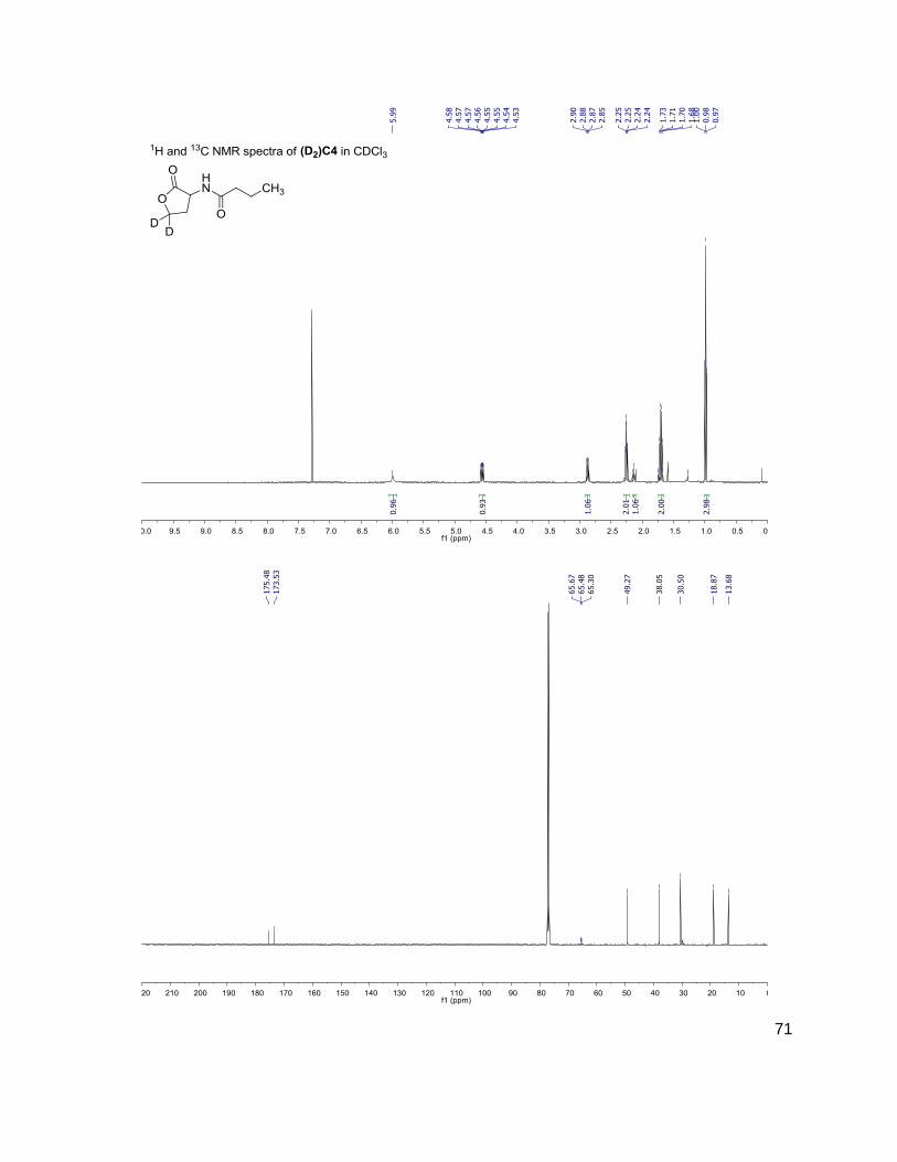
71

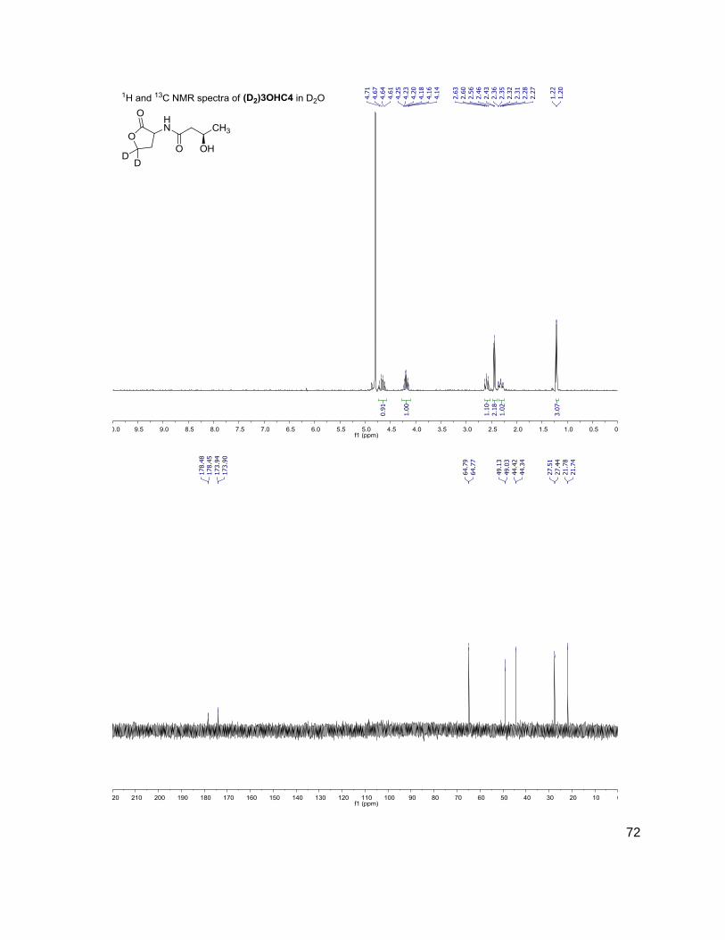
72

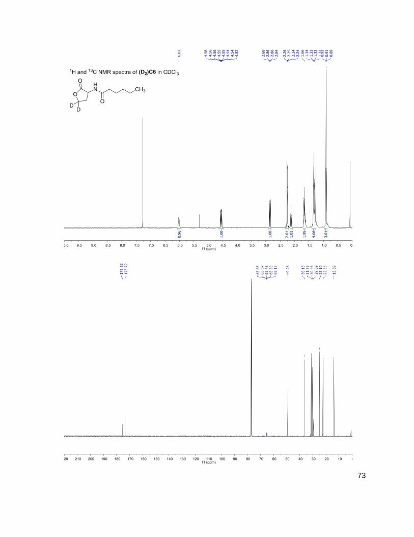
73

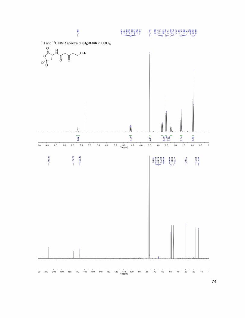
74

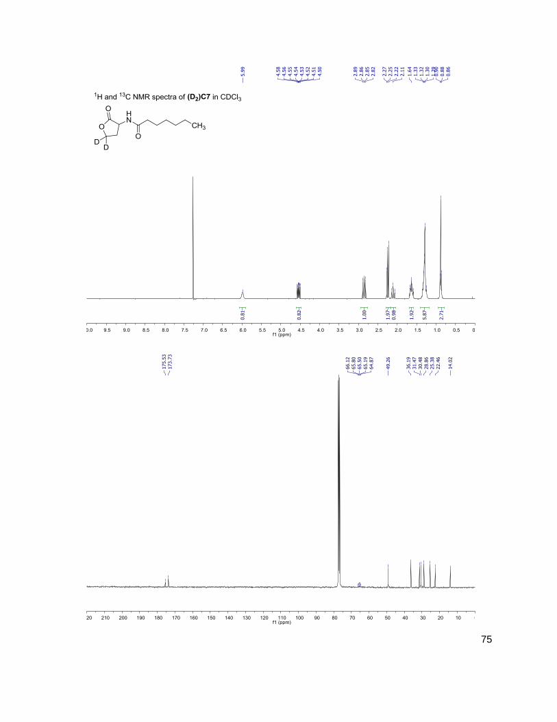
75

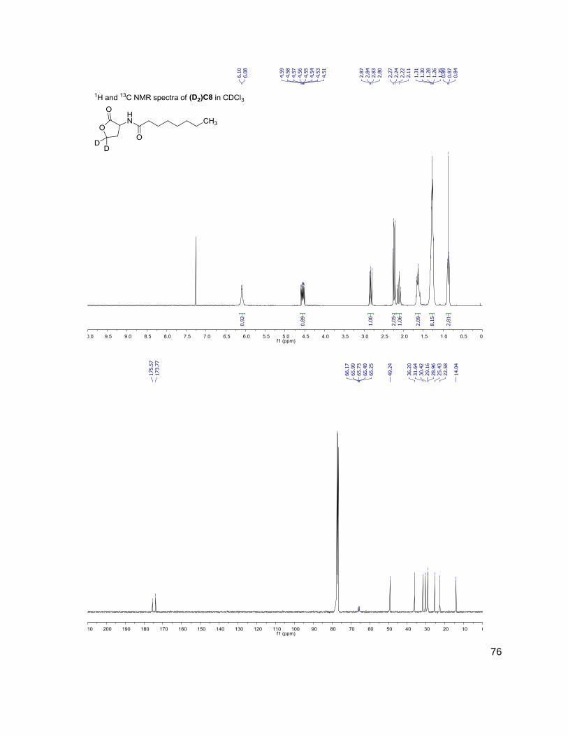
76

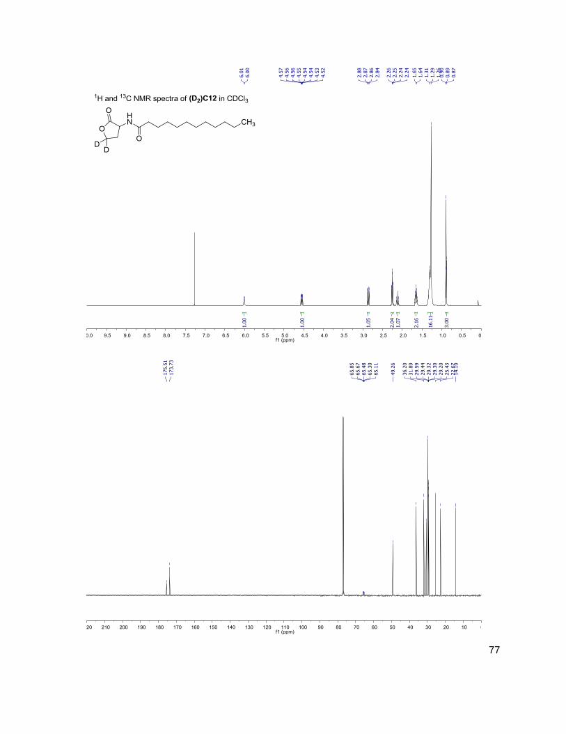
77

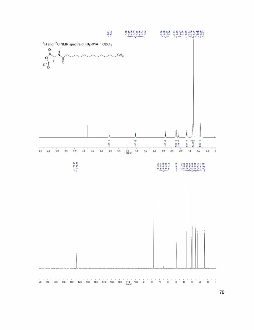
78

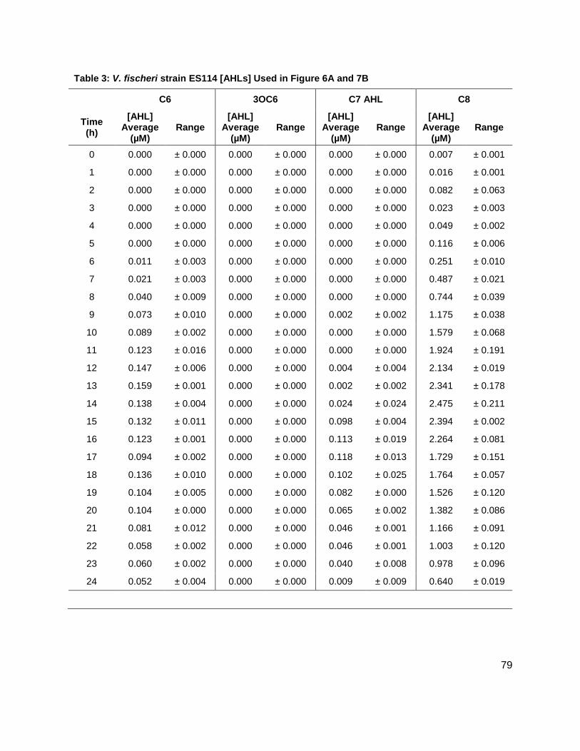
79

Table 3: V. fischeri strain ES114 [AHLs] Used in Figure 6A and 7B

C6 3OC6 C7 AHL C8

Time (h)

[AHL] Average

(µM) Range

[AHL] Average

(µM) Range

[AHL] Average

(µM) Range

[AHL] Average

(µM) Range

0 0.000 ± 0.000 0.000 ± 0.000 0.000 ± 0.000 0.007 ± 0.001

1 0.000 ± 0.000 0.000 ± 0.000 0.000 ± 0.000 0.016 ± 0.001

2 0.000 ± 0.000 0.000 ± 0.000 0.000 ± 0.000 0.082 ± 0.063

3 0.000 ± 0.000 0.000 ± 0.000 0.000 ± 0.000 0.023 ± 0.003

4 0.000 ± 0.000 0.000 ± 0.000 0.000 ± 0.000 0.049 ± 0.002

5 0.000 ± 0.000 0.000 ± 0.000 0.000 ± 0.000 0.116 ± 0.006

6 0.011 ± 0.003 0.000 ± 0.000 0.000 ± 0.000 0.251 ± 0.010

7 0.021 ± 0.003 0.000 ± 0.000 0.000 ± 0.000 0.487 ± 0.021

8 0.040 ± 0.009 0.000 ± 0.000 0.000 ± 0.000 0.744 ± 0.039

9 0.073 ± 0.010 0.000 ± 0.000 0.002 ± 0.002 1.175 ± 0.038

10 0.089 ± 0.002 0.000 ± 0.000 0.000 ± 0.000 1.579 ± 0.068

11 0.123 ± 0.016 0.000 ± 0.000 0.000 ± 0.000 1.924 ± 0.191

12 0.147 ± 0.006 0.000 ± 0.000 0.004 ± 0.004 2.134 ± 0.019

13 0.159 ± 0.001 0.000 ± 0.000 0.002 ± 0.002 2.341 ± 0.178

14 0.138 ± 0.004 0.000 ± 0.000 0.024 ± 0.024 2.475 ± 0.211

15 0.132 ± 0.011 0.000 ± 0.000 0.098 ± 0.004 2.394 ± 0.002

16 0.123 ± 0.001 0.000 ± 0.000 0.113 ± 0.019 2.264 ± 0.081

17 0.094 ± 0.002 0.000 ± 0.000 0.118 ± 0.013 1.729 ± 0.151

18 0.136 ± 0.010 0.000 ± 0.000 0.102 ± 0.025 1.764 ± 0.057

19 0.104 ± 0.005 0.000 ± 0.000 0.082 ± 0.000 1.526 ± 0.120

20 0.104 ± 0.000 0.000 ± 0.000 0.065 ± 0.002 1.382 ± 0.086

21 0.081 ± 0.012 0.000 ± 0.000 0.046 ± 0.001 1.166 ± 0.091

22 0.058 ± 0.002 0.000 ± 0.000 0.046 ± 0.001 1.003 ± 0.120

23 0.060 ± 0.002 0.000 ± 0.000 0.040 ± 0.008 0.978 ± 0.096

24 0.052 ± 0.004 0.000 ± 0.000 0.009 ± 0.009 0.640 ± 0.019

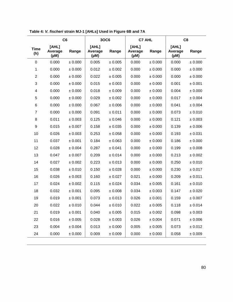
80

Table 4: V. fischeri strain MJ-1 [AHLs] Used in Figure 6B and 7A

C6 3OC6 C7 AHL C8

Time (h)

[AHL] Average

(µM) Range

[AHL] Average

(µM) Range

[AHL] Average

(µM) Range

[AHL] Average

(µM) Range

0 0.000 ± 0.000 0.005 ± 0.005 0.000 ± 0.000 0.000 ± 0.000

1 0.000 ± 0.000 0.012 ± 0.002 0.000 ± 0.000 0.000 ± 0.000

2 0.000 ± 0.000 0.022 ± 0.005 0.000 ± 0.000 0.000 ± 0.000

3 0.000 ± 0.000 0.015 ± 0.003 0.000 ± 0.000 0.001 ± 0.001

4 0.000 ± 0.000 0.018 ± 0.009 0.000 ± 0.000 0.004 ± 0.000

5 0.000 ± 0.000 0.029 ± 0.002 0.000 ± 0.000 0.017 ± 0.004

6 0.000 ± 0.000 0.067 ± 0.006 0.000 ± 0.000 0.041 ± 0.004

7 0.000 ± 0.000 0.091 ± 0.011 0.000 ± 0.000 0.073 ± 0.010

8 0.011 ± 0.003 0.125 ± 0.046 0.000 ± 0.000 0.121 ± 0.003

9 0.015 ± 0.007 0.158 ± 0.035 0.000 ± 0.000 0.139 ± 0.006

10 0.026 ± 0.003 0.253 ± 0.058 0.000 ± 0.000 0.193 ± 0.031

11 0.037 ± 0.001 0.184 ± 0.063 0.000 ± 0.000 0.186 ± 0.000

12 0.028 ± 0.004 0.287 ± 0.041 0.000 ± 0.000 0.199 ± 0.008

13 0.047 ± 0.007 0.209 ± 0.014 0.000 ± 0.000 0.213 ± 0.002

14 0.027 ± 0.002 0.223 ± 0.013 0.000 ± 0.000 0.250 ± 0.010

15 0.038 ± 0.010 0.150 ± 0.028 0.000 ± 0.000 0.230 ± 0.017

16 0.026 ± 0.003 0.160 ± 0.027 0.021 ± 0.000 0.209 ± 0.011

17 0.024 ± 0.002 0.115 ± 0.024 0.034 ± 0.005 0.161 ± 0.010

18 0.032 ± 0.001 0.095 ± 0.008 0.034 ± 0.003 0.147 ± 0.020

19 0.019 ± 0.001 0.073 ± 0.013 0.026 ± 0.001 0.159 ± 0.007

20 0.022 ± 0.010 0.044 ± 0.010 0.022 ± 0.005 0.118 ± 0.014

21 0.019 ± 0.001 0.040 ± 0.005 0.015 ± 0.002 0.098 ± 0.003

22 0.016 ± 0.005 0.028 ± 0.003 0.026 ± 0.004 0.071 ± 0.006

23 0.004 ± 0.004 0.013 ± 0.000 0.005 ± 0.005 0.073 ± 0.012

24 0.000 ± 0.000 0.009 ± 0.009 0.000 ± 0.000 0.058 ± 0.009

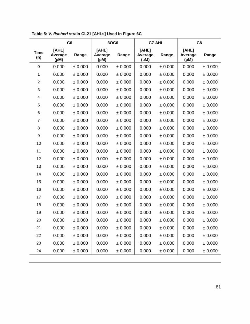
81

Table 5: V. fischeri strain CL21 [AHLs] Used in Figure 6C

C6 3OC6 C7 AHL C8

Time (h)

[AHL] Average

(µM) Range

[AHL] Average

(µM) Range

[AHL] Average

(µM) Range

[AHL] Average

(µM) Range

0 0.000 ± 0.000 0.000 ± 0.000 0.000 ± 0.000 0.000 ± 0.000

1 0.000 ± 0.000 0.000 ± 0.000 0.000 ± 0.000 0.000 ± 0.000

2 0.000 ± 0.000 0.000 ± 0.000 0.000 ± 0.000 0.000 ± 0.000

3 0.000 ± 0.000 0.000 ± 0.000 0.000 ± 0.000 0.000 ± 0.000

4 0.000 ± 0.000 0.000 ± 0.000 0.000 ± 0.000 0.000 ± 0.000

5 0.000 ± 0.000 0.000 ± 0.000 0.000 ± 0.000 0.000 ± 0.000

6 0.000 ± 0.000 0.000 ± 0.000 0.000 ± 0.000 0.000 ± 0.000

7 0.000 ± 0.000 0.000 ± 0.000 0.000 ± 0.000 0.000 ± 0.000

8 0.000 ± 0.000 0.000 ± 0.000 0.000 ± 0.000 0.000 ± 0.000

9 0.000 ± 0.000 0.000 ± 0.000 0.000 ± 0.000 0.000 ± 0.000

10 0.000 ± 0.000 0.000 ± 0.000 0.000 ± 0.000 0.000 ± 0.000

11 0.000 ± 0.000 0.000 ± 0.000 0.000 ± 0.000 0.000 ± 0.000

12 0.000 ± 0.000 0.000 ± 0.000 0.000 ± 0.000 0.000 ± 0.000

13 0.000 ± 0.000 0.000 ± 0.000 0.000 ± 0.000 0.000 ± 0.000

14 0.000 ± 0.000 0.000 ± 0.000 0.000 ± 0.000 0.000 ± 0.000

15 0.000 ± 0.000 0.000 ± 0.000 0.000 ± 0.000 0.000 ± 0.000

16 0.000 ± 0.000 0.000 ± 0.000 0.000 ± 0.000 0.000 ± 0.000

17 0.000 ± 0.000 0.000 ± 0.000 0.000 ± 0.000 0.000 ± 0.000

18 0.000 ± 0.000 0.000 ± 0.000 0.000 ± 0.000 0.000 ± 0.000

19 0.000 ± 0.000 0.000 ± 0.000 0.000 ± 0.000 0.000 ± 0.000

20 0.000 ± 0.000 0.000 ± 0.000 0.000 ± 0.000 0.000 ± 0.000

21 0.000 ± 0.000 0.000 ± 0.000 0.000 ± 0.000 0.000 ± 0.000

22 0.000 ± 0.000 0.000 ± 0.000 0.000 ± 0.000 0.000 ± 0.000

23 0.000 ± 0.000 0.000 ± 0.000 0.000 ± 0.000 0.000 ± 0.000

24 0.000 ± 0.000 0.000 ± 0.000 0.000 ± 0.000 0.000 ± 0.000

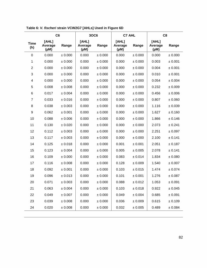
82

Table 6: V. fischeri strain VCW2G7 [AHLs] Used in Figure 6D

C6 3OC6 C7 AHL C8

Time (h)

[AHL] Average

(µM) Range

[AHL] Average

(µM) Range

[AHL] Average

(µM) Range

[AHL] Average

(µM) Range

0 0.000 ± 0.000 0.000 ± 0.000 0.000 ± 0.000 0.000 ± 0.000

1 0.000 ± 0.000 0.000 ± 0.000 0.000 ± 0.000 0.003 ± 0.001

2 0.000 ± 0.000 0.000 ± 0.000 0.000 ± 0.000 0.004 ± 0.001

3 0.000 ± 0.000 0.000 ± 0.000 0.000 ± 0.000 0.010 ± 0.001

4 0.000 ± 0.000 0.000 ± 0.000 0.000 ± 0.000 0.054 ± 0.004

5 0.008 ± 0.008 0.000 ± 0.000 0.000 ± 0.000 0.232 ± 0.009

6 0.017 ± 0.004 0.000 ± 0.000 0.000 ± 0.000 0.456 ± 0.006

7 0.033 ± 0.016 0.000 ± 0.000 0.000 ± 0.000 0.807 ± 0.060

8 0.038 ± 0.003 0.000 ± 0.000 0.000 ± 0.000 1.116 ± 0.039

9 0.062 ± 0.001 0.000 ± 0.000 0.000 ± 0.000 1.627 ± 0.160

10 0.088 ± 0.006 0.000 ± 0.000 0.000 ± 0.000 1.866 ± 0.146

11 0.130 ± 0.020 0.000 ± 0.000 0.000 ± 0.000 2.073 ± 0.241

12 0.112 ± 0.003 0.000 ± 0.000 0.000 ± 0.000 2.251 ± 0.097

13 0.117 ± 0.003 0.000 ± 0.000 0.000 ± 0.000 2.100 ± 0.141

14 0.125 ± 0.018 0.000 ± 0.000 0.001 ± 0.001 2.051 ± 0.187

15 0.123 ± 0.004 0.000 ± 0.000 0.005 ± 0.005 2.078 ± 0.141

16 0.109 ± 0.000 0.000 ± 0.000 0.083 ± 0.014 1.834 ± 0.080

17 0.116 ± 0.008 0.000 ± 0.000 0.128 ± 0.009 1.540 ± 0.007

18 0.092 ± 0.001 0.000 ± 0.000 0.103 ± 0.015 1.474 ± 0.074

19 0.096 ± 0.013 0.000 ± 0.000 0.101 ± 0.001 1.276 ± 0.087

20 0.071 ± 0.003 0.000 ± 0.000 0.088 ± 0.012 1.053 ± 0.091

21 0.063 ± 0.004 0.000 ± 0.000 0.103 ± 0.018 0.922 ± 0.045

22 0.049 ± 0.007 0.000 ± 0.000 0.049 ± 0.004 0.685 ± 0.091

23 0.039 ± 0.008 0.000 ± 0.000 0.036 ± 0.009 0.615 ± 0.109

24 0.020 ± 0.008 0.000 ± 0.000 0.032 ± 0.005 0.489 ± 0.084

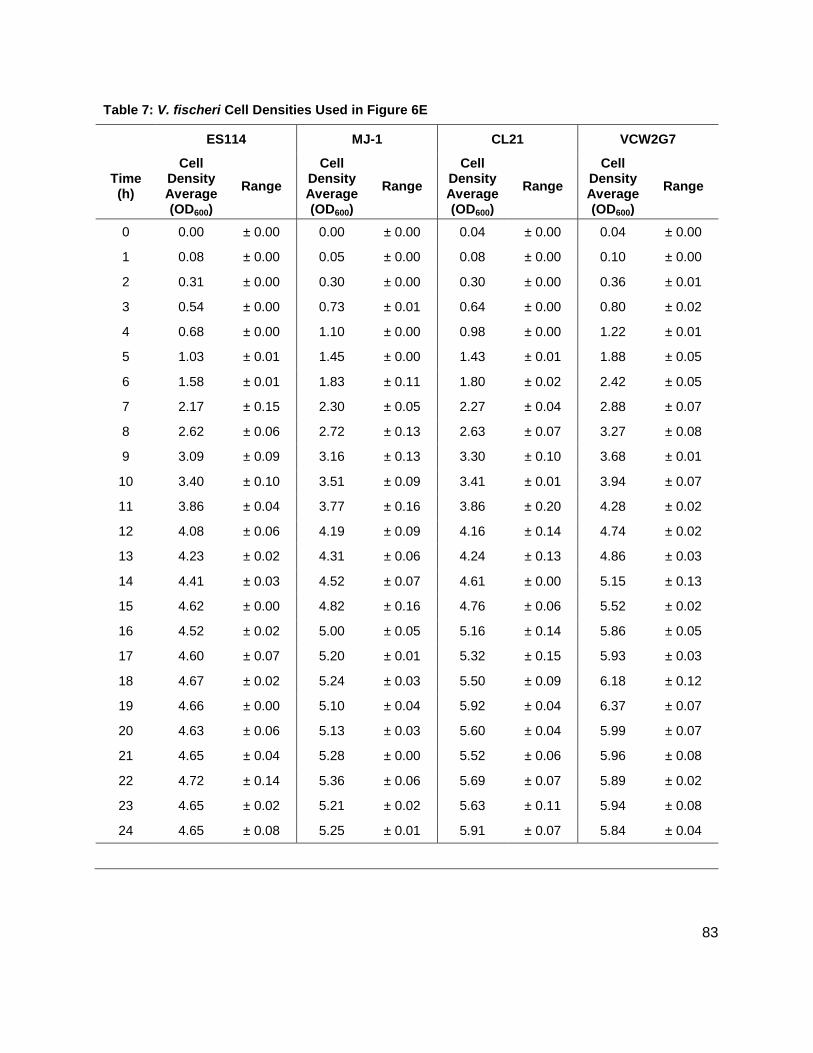
83

Table 7: V. fischeri Cell Densities Used in Figure 6E

ES114 MJ-1 CL21 VCW2G7

Time (h)

Cell Density Average (OD600)

Range


Range


Range


Range

0 0.00 ± 0.00 0.00 ± 0.00 0.04 ± 0.00 0.04 ± 0.00

1 0.08 ± 0.00 0.05 ± 0.00 0.08 ± 0.00 0.10 ± 0.00

2 0.31 ± 0.00 0.30 ± 0.00 0.30 ± 0.00 0.36 ± 0.01

3 0.54 ± 0.00 0.73 ± 0.01 0.64 ± 0.00 0.80 ± 0.02

4 0.68 ± 0.00 1.10 ± 0.00 0.98 ± 0.00 1.22 ± 0.01

5 1.03 ± 0.01 1.45 ± 0.00 1.43 ± 0.01 1.88 ± 0.05

6 1.58 ± 0.01 1.83 ± 0.11 1.80 ± 0.02 2.42 ± 0.05

7 2.17 ± 0.15 2.30 ± 0.05 2.27 ± 0.04 2.88 ± 0.07

8 2.62 ± 0.06 2.72 ± 0.13 2.63 ± 0.07 3.27 ± 0.08

9 3.09 ± 0.09 3.16 ± 0.13 3.30 ± 0.10 3.68 ± 0.01

10 3.40 ± 0.10 3.51 ± 0.09 3.41 ± 0.01 3.94 ± 0.07

11 3.86 ± 0.04 3.77 ± 0.16 3.86 ± 0.20 4.28 ± 0.02

12 4.08 ± 0.06 4.19 ± 0.09 4.16 ± 0.14 4.74 ± 0.02

13 4.23 ± 0.02 4.31 ± 0.06 4.24 ± 0.13 4.86 ± 0.03

14 4.41 ± 0.03 4.52 ± 0.07 4.61 ± 0.00 5.15 ± 0.13

15 4.62 ± 0.00 4.82 ± 0.16 4.76 ± 0.06 5.52 ± 0.02

16 4.52 ± 0.02 5.00 ± 0.05 5.16 ± 0.14 5.86 ± 0.05

17 4.60 ± 0.07 5.20 ± 0.01 5.32 ± 0.15 5.93 ± 0.03

18 4.67 ± 0.02 5.24 ± 0.03 5.50 ± 0.09 6.18 ± 0.12

19 4.66 ± 0.00 5.10 ± 0.04 5.92 ± 0.04 6.37 ± 0.07

20 4.63 ± 0.06 5.13 ± 0.03 5.60 ± 0.04 5.99 ± 0.07

21 4.65 ± 0.04 5.28 ± 0.00 5.52 ± 0.06 5.96 ± 0.08

22 4.72 ± 0.14 5.36 ± 0.06 5.69 ± 0.07 5.89 ± 0.02

23 4.65 ± 0.02 5.21 ± 0.02 5.63 ± 0.11 5.94 ± 0.08

24 4.65 ± 0.08 5.25 ± 0.01 5.91 ± 0.07 5.84 ± 0.04

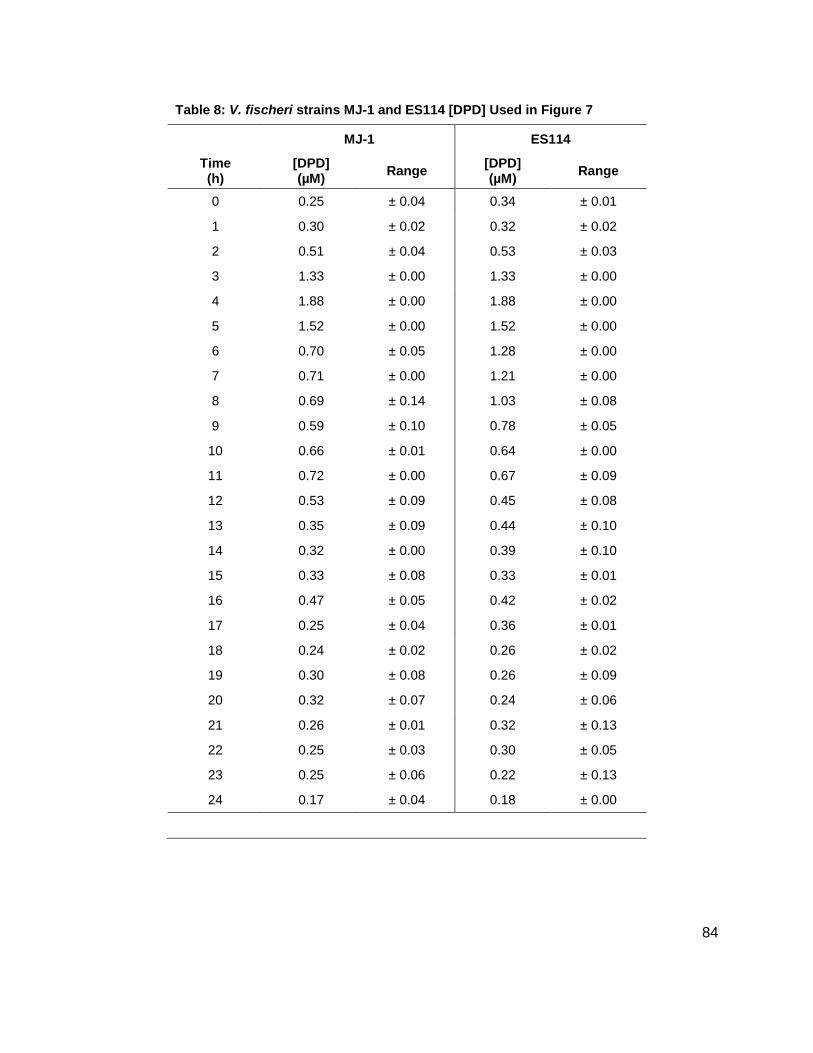
84

Table 8: V. fischeri strains MJ-1 and ES114 [DPD] Used in Figure 7

MJ-1 ES114

Time (h)

[DPD] (µM)

Range [DPD] (µM)

Range

0 0.25 ± 0.04 0.34 ± 0.01

1 0.30 ± 0.02 0.32 ± 0.02

2 0.51 ± 0.04 0.53 ± 0.03

3 1.33 ± 0.00 1.33 ± 0.00

4 1.88 ± 0.00 1.88 ± 0.00

5 1.52 ± 0.00 1.52 ± 0.00

6 0.70 ± 0.05 1.28 ± 0.00

7 0.71 ± 0.00 1.21 ± 0.00

8 0.69 ± 0.14 1.03 ± 0.08

9 0.59 ± 0.10 0.78 ± 0.05

10 0.66 ± 0.01 0.64 ± 0.00

11 0.72 ± 0.00 0.67 ± 0.09

12 0.53 ± 0.09 0.45 ± 0.08

13 0.35 ± 0.09 0.44 ± 0.10

14 0.32 ± 0.00 0.39 ± 0.10

15 0.33 ± 0.08 0.33 ± 0.01

16 0.47 ± 0.05 0.42 ± 0.02

17 0.25 ± 0.04 0.36 ± 0.01

18 0.24 ± 0.02 0.26 ± 0.02

19 0.30 ± 0.08 0.26 ± 0.09

20 0.32 ± 0.07 0.24 ± 0.06

21 0.26 ± 0.01 0.32 ± 0.13

22 0.25 ± 0.03 0.30 ± 0.05

23 0.25 ± 0.06 0.22 ± 0.13

24 0.17 ± 0.04 0.18 ± 0.00

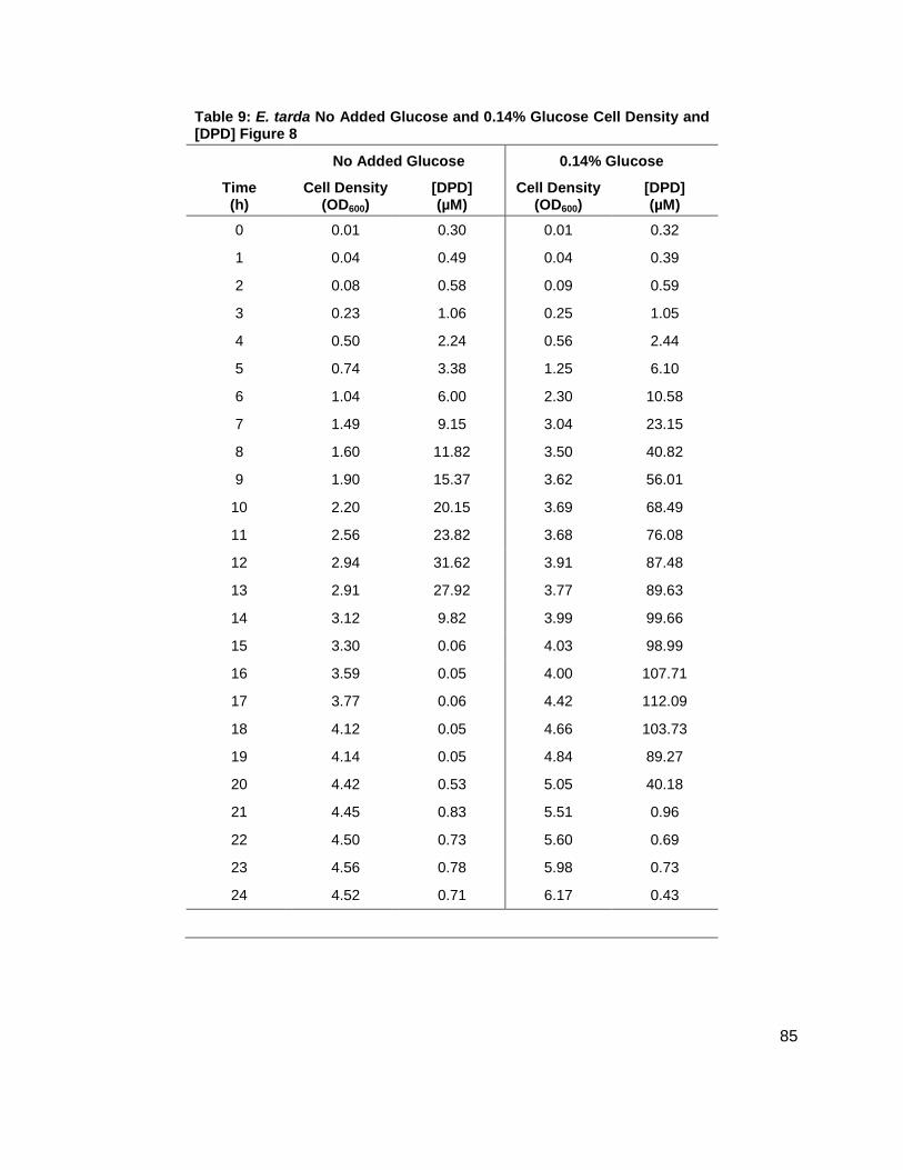
85

Table 9: E. tarda No Added Glucose and 0.14% Glucose Cell Density and [DPD] Figure 8

No Added Glucose 0.14% Glucose

Time (h)

Cell Density (OD600)

[DPD] (µM)

Cell Density (OD600)

[DPD] (µM)

0 0.01 0.30 0.01 0.32

1 0.04 0.49 0.04 0.39

2 0.08 0.58 0.09 0.59

3 0.23 1.06 0.25 1.05

4 0.50 2.24 0.56 2.44

5 0.74 3.38 1.25 6.10

6 1.04 6.00 2.30 10.58

7 1.49 9.15 3.04 23.15

8 1.60 11.82 3.50 40.82

9 1.90 15.37 3.62 56.01

10 2.20 20.15 3.69 68.49

11 2.56 23.82 3.68 76.08

12 2.94 31.62 3.91 87.48

13 2.91 27.92 3.77 89.63

14 3.12 9.82 3.99 99.66

15 3.30 0.06 4.03 98.99

16 3.59 0.05 4.00 107.71

17 3.77 0.06 4.42 112.09

18 4.12 0.05 4.66 103.73

19 4.14 0.05 4.84 89.27

20 4.42 0.53 5.05 40.18

21 4.45 0.83 5.51 0.96

22 4.50 0.73 5.60 0.69

23 4.56 0.78 5.98 0.73

24 4.52 0.71 6.17 0.43

86

Table 10: Y. enterocolitica No Added Glucose Cell Density and [DPD]/OD Used in Figure 9

Time (h)


Range

[DPD]/OD Average

(M/OD600)

Range

1 0.03 ± 0.00 25.13 ± 0.66

2 0.07 ± 0.00 13.78 ± 0.22

3 0.14 ± 0.00 7.44 ± 0.21

4 0.31 ± 0.00 4.72 ± 0.10

5 0.52 ± 0.02 4.41 ± 0.11

6 0.95 ± 0.01 4.82 ± 0.02

7 1.68 ± 0.03 6.06 ± 0.09

8 2.25 ± 0.06 11.43 ± 0.31

9 2.40 ± 0.15 22.45 ± 0.93

10 2.94 ± 0.05 26.75 ± 0.54

11 3.26 ± 0.13 20.44 ± 1.22

12 3.46 ± 0.14 8.53 ± 0.18

13 3.69 ± 0.10 0.17 ± 0.14

14 3.79 ± 0.11 0.13 ± 0.11

15 4.05 ± 0.05 0.09 ± 0.08

16 4.05 ± 0.05 0.08 ± 0.07

87

Table 11: Y. enterocolitica 0.08% Glucose Cell Density and [DPD]/OD Used in Figure 9

Time (h)


Range

[DPD]/OD Average

(M/OD600)

Range

1 0.03 ± 0.00 26.48 ± 0.05

2 0.07 ± 0.00 13.75 ± 0.32

3 0.14 ± 0.00 7.49 ± 0.17

4 0.31 ± 0.01 4.74 ± 0.07

5 0.51 ± 0.01 4.34 ± 0.17

6 0.90 ± 0.02 4.80 ± 0.05

7 1.53 ± 0.05 6.22 ± 0.03

8 2.00 ± 0.04 11.68 ± 0.39

9 2.19 ± 0.06 24.32 ± 0.02

10 2.63 ± 0.15 34.15 ± 0.47

11 2.99 ± 0.08 36.54 ± 0.39

12 3.50 ± 0.14 24.61 ± 1.38

13 3.73 ± 0.01 8.49 ± 0.19

14 4.02 ± 0.02 0.34 ± 0.01

15 4.22 ± 0.02 0.24 ± 0.00

16 4.22 ± 0.02 0.22 ± 0.04

88


Time (h)


Range

[DPD]/OD Average

(M/OD600)

Range

1 0.03 ± 0.00 45.97 ± 6.89

2 0.05 ± 0.00 22.07 ± 2.99

3 0.11 ± 0.00 10.97 ± 0.35

4 0.25 ± 0.01 5.80 ± 0.10

5 0.46 ± 0.01 4.71 ± 0.05

6 0.86 ± 0.01 4.80 ± 0.11

7 1.71 ± 0.00 5.48 ± 0.28

8 2.19 ± 0.04 10.10 ± 0.73

9 2.69 ± 0.03 18.53 ± 1.00

10 3.13 ± 0.03 27.53 ± 1.21

11 3.52 ± 0.04 31.50 ± 0.39

12 3.88 ± 0.01 20.17 ± 0.85

13 4.20 ± 0.07 2.76 ± 1.05

14 4.37 ± 0.03 0.51 ± 0.04

15 4.63 ± 0.05 0.31 ± 0.03

16 4.89 ± 0.06 0.32 ± 0.05

89


Time (h)


Range

[DPD]/OD Average

(M/OD600)

Range

1 0.03 ± 0.00 38.42 ± 1.50

2 0.05 ± 0.00 19.17 ± 0.49

3 0.12 ± 0.00 10.17 ± 0.16

4 0.25 ± 0.00 5.86 ± 0.11

5 0.47 ± 0.00 4.83 ± 0.03

6 0.87 ± 0.01 4.96 ± 0.01

7 1.73 ± 0.03 5.72 ± 0.02

8 2.20 ± 0.00 10.18 ± 0.14

9 2.67 ± 0.02 20.07 ± 0.44

10 3.11 ± 0.02 27.86 ± 0.21

11 3.60 ± 0.05 31.98 ± 1.56

12 3.96 ± 0.05 24.58 ± 0.74

13 4.30 ± 0.05 5.89 ± 0.66

14 4.47 ± 0.02 0.45 ± 0.00

15 4.72 ± 0.04 0.34 ± 0.00

16 5.03 ± 0.02 0.24 ± 0.01

90

Table 14: Y. enterocolitica No Added Glucose [DPD] and % Glucose Used in Figure 10A

Time (h)

[DPD] Average

(M)

Range % Glucose

Average (% (w/v))

Range

0 0.78 ± 0.02 0.15 ± 0.01

1 0.84 ± 0.02 0.14 ± 0.01

2 0.91 ± 0.01 0.12 ± 0.00

3 1.05 ± 0.00 0.11 ± 0.00

4 1.47 ± 0.01 0.10 ± 0.00

5 2.31 ± 0.01 0.08 ± 0.00

6 4.56 ± 0.04 0.08 ± 0.00

7 10.18 ± 0.07 0.07 ± 0.01

8 25.71 ± 0.02 0.02 ± 0.00

9 53.69 ± 1.19 -0.01 ± 0.00

10 78.62 ± 0.24 -0.01 ± 0.00

11 66.37 ± 1.31 -0.01 ± 0.00

12 29.48 ± 0.59 -0.01 ± 0.00

13 0.63 ± 0.51 -0.01 ± 0.00

14 0.47 ± 0.39 -0.01 ± 0.00

15 0.37 ± 0.31 0.00 ± 0.00

16 0.33 ± 0.27 -0.01 ± 0.00

A500 = 6.808 [ ] + 0.4399; R² = 0.9938

91

Table 15: Y. enterocolitica 0.08% Glucose [DPD] and % Glucose Used in Figure 10B

Time (h)

[DPD] Average

(M)

Range % Glucose

Average (% (w/v))

Range

0 0.78 ± 0.01 0.12 ± 0.01

1 0.81 ± 0.01 0.10 ± 0.01

2 0.91 ± 0.01 0.10 ± 0.01

3 1.02 ± 0.04 0.10 ± 0.02

4 1.45 ± 0.00 0.10 ± 0.01

5 2.20 ± 0.13 0.10 ± 0.02

6 4.32 ± 0.13 0.10 ± 0.01

7 9.48 ± 0.24 0.11 ± 0.01

8 23.31 ± 1.24 0.08 ± 0.02

9 53.13 ± 1.29 0.04 ± 0.02

10 89.75 ± 3.89 0.00 ± 0.01

11 109.14 ± 1.66 0.01 ± 0.02

12 85.84 ± 1.51 0.00 ± 0.02

13 31.63 ± 0.68 0.00 ± 0.01

14 1.37 ± 0.03 0.00 ± 0.01

15 0.99 ± 0.00 0.00 ± 0.01

16 0.93 ± 0.15 0.00 ± 0.01

A500 = 5.869 [ ] + 0.2882; R² = 0.9849

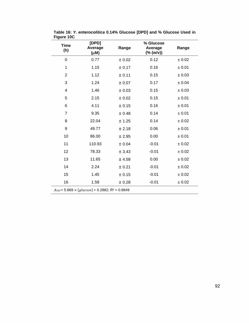
92

Table 16: Y. enterocolitica 0.14% Glucose [DPD] and % Glucose Used in Figure 10C

Time (h)

[DPD] Average

(M)

Range % Glucose

Average (% (w/v))

Range

0 0.77 ± 0.02 0.12 ± 0.02

1 1.15 ± 0.17 0.16 ± 0.01

2 1.12 ± 0.11 0.15 ± 0.03

3 1.24 ± 0.07 0.17 ± 0.04

4 1.46 ± 0.03 0.15 ± 0.03

5 2.15 ± 0.02 0.15 ± 0.01

6 4.11 ± 0.15 0.16 ± 0.01

7 9.35 ± 0.48 0.14 ± 0.01

8 22.04 ± 1.25 0.14 ± 0.02

9 49.77 ± 2.18 0.06 ± 0.01

10 86.00 ± 2.95 0.00 ± 0.01

11 110.93 ± 0.04 -0.01 ± 0.02

12 78.33 ± 3.43 -0.01 ± 0.02

13 11.65 ± 4.58 0.00 ± 0.02

14 2.24 ± 0.21 -0.01 ± 0.02

15 1.45 ± 0.15 -0.01 ± 0.02

16 1.58 ± 0.28 -0.01 ± 0.02

A500 = 5.869 [ ] + 0.2882; R² = 0.9849

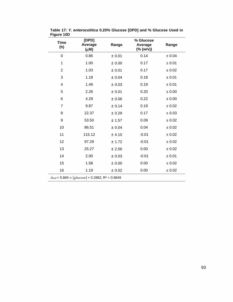
93

Table 17: Y. enterocolitica 0.20% Glucose [DPD] and % Glucose Used in Figure 10D

Time (h)

[DPD] Average

(M)

Range % Glucose

Average (% (w/v))

Range

0 0.86 ± 0.01 0.14 ± 0.04

1 1.00 ± 0.00 0.17 ± 0.01

2 1.03 ± 0.01 0.17 ± 0.02

3 1.18 ± 0.04 0.18 ± 0.01

4 1.49 ± 0.03 0.19 ± 0.01

5 2.26 ± 0.01 0.20 ± 0.00

6 4.29 ± 0.06 0.22 ± 0.00

7 9.87 ± 0.14 0.19 ± 0.02

8 22.37 ± 0.29 0.17 ± 0.03

9 53.50 ± 1.57 0.09 ± 0.02

10 86.51 ± 0.04 0.04 ± 0.02

11 115.12 ± 4.10 -0.01 ± 0.02

12 97.29 ± 1.72 -0.01 ± 0.02

13 25.27 ± 2.56 0.00 ± 0.02

14 2.00 ± 0.03 -0.01 ± 0.01

15 1.58 ± 0.00 0.00 ± 0.02

16 1.19 ± 0.02 0.00 ± 0.02

A500 = 5.869 [ ] + 0.2882; R² = 0.9849

94

Table 18: Y. enterocolitica No Added Glucose Cell Density and [DPD]/OD Used in Figure 11

Time (h)


Range

[DPD]/OD Average

(M/OD600)

Range

1 0.02 ± 0.00 18.35 ± 0.87

2 0.04 ± 0.00 10.41 ± 0.41

3 0.11 ± 0.00 5.48 ± 0.05

4 0.24 ± 0.02 4.16 ± 0.38

5 0.52 ± 0.01 4.14 ± 0.13

6 0.82 ± 0.05 5.84 ± 0.22

7 1.50 ± 0.04 6.00 ± 0.35

8 1.73 ± 0.06 6.39 ± 0.38

9 1.92 ± 0.09 4.95 ± 0.16

10 2.25 ± 0.11 1.62 ± 0.20

11 2.54 ± 0.09 0.27 ± 0.00

12 2.84 ± 0.09 0.20 ± 0.00

13 3.11 ± 0.10 0.18 ± 0.01

14 3.48 ± 0.07 0.17 ± 0.01

15 3.72 ± 0.16 0.14 ± 0.01

16 4.03 ± 0.10 0.12 ± 0.00

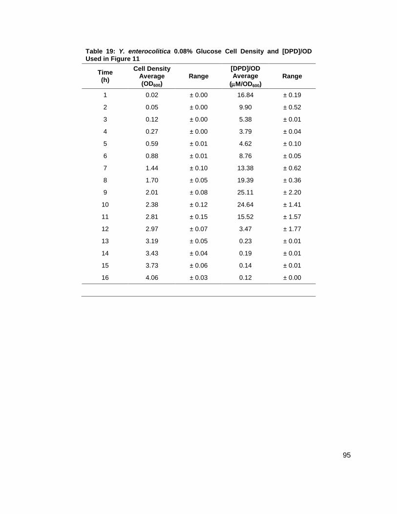
95


Time (h)


Range

[DPD]/OD Average

(M/OD600)

Range

1 0.02 ± 0.00 16.84 ± 0.19

2 0.05 ± 0.00 9.90 ± 0.52

3 0.12 ± 0.00 5.38 ± 0.01

4 0.27 ± 0.00 3.79 ± 0.04

5 0.59 ± 0.01 4.62 ± 0.10

6 0.88 ± 0.01 8.76 ± 0.05

7 1.44 ± 0.10 13.38 ± 0.62

8 1.70 ± 0.05 19.39 ± 0.36

9 2.01 ± 0.08 25.11 ± 2.20

10 2.38 ± 0.12 24.64 ± 1.41

11 2.81 ± 0.15 15.52 ± 1.57

12 2.97 ± 0.07 3.47 ± 1.77

13 3.19 ± 0.05 0.23 ± 0.01

14 3.43 ± 0.04 0.19 ± 0.01

15 3.73 ± 0.06 0.14 ± 0.01

16 4.06 ± 0.03 0.12 ± 0.00

96


Time (h)


Range

[DPD]/OD Average

(M/OD600)

Range

1 0.02 ± 0.00 23.59 ± 0.95

2 0.05 ± 0.00 11.45 ± 0.04

3 0.13 ± 0.00 5.11 ± 0.15

4 0.32 ± 0.01 3.86 ± 0.05

5 0.66 ± 0.02 4.83 ± 0.05

6 1.08 ± 0.01 7.51 ± 0.14

7 1.70 ± 0.00 11.26 ± 0.25

8 1.95 ± 0.08 18.71 ± 0.68

9 2.32 ± 0.03 25.04 ± 1.06

10 2.62 ± 0.04 28.56 ± 0.07

11 3.02 ± 0.05 25.34 ± 0.96

12 3.29 ± 0.04 16.24 ± 0.57

13 3.38 ± 0.01 6.97 ± 0.43

14 3.42 ± 0.01 0.27 ± 0.01

15 3.64 ± 0.00 0.21 ± 0.02

16 3.92 ± 0.06 0.18 ± 0.01

97


Time (h)


Range

[DPD]/OD Average

(M/OD600)

Range

1 0.02 ± 0.00 24.32 ± 0.39

2 0.05 ± 0.00 10.33 ± 0.04

3 0.13 ± 0.00 5.51 ± 0.08

4 0.31 ± 0.01 3.86 ± 0.16

5 0.67 ± 0.00 4.60 ± 0.04

6 1.10 ± 0.02 7.79 ± 0.33

7 1.68 ± 0.00 11.81 ± 0.32

8 1.98 ± 0.02 18.58 ± 0.58

9 2.38 ± 0.02 26.89 ± 0.08

10 2.62 ± 0.07 32.92 ± 0.37

11 3.01 ± 0.08 32.36 ± 1.12

12 3.31 ± 0.06 26.24 ± 1.07

13 3.49 ± 0.13 18.55 ± 2.00

14 3.55 ± 0.11 7.56 ± 1.65

15 3.47 ± 0.41 0.29 ± 0.01

16 4.03 ± 0.19 0.21 ± 0.00

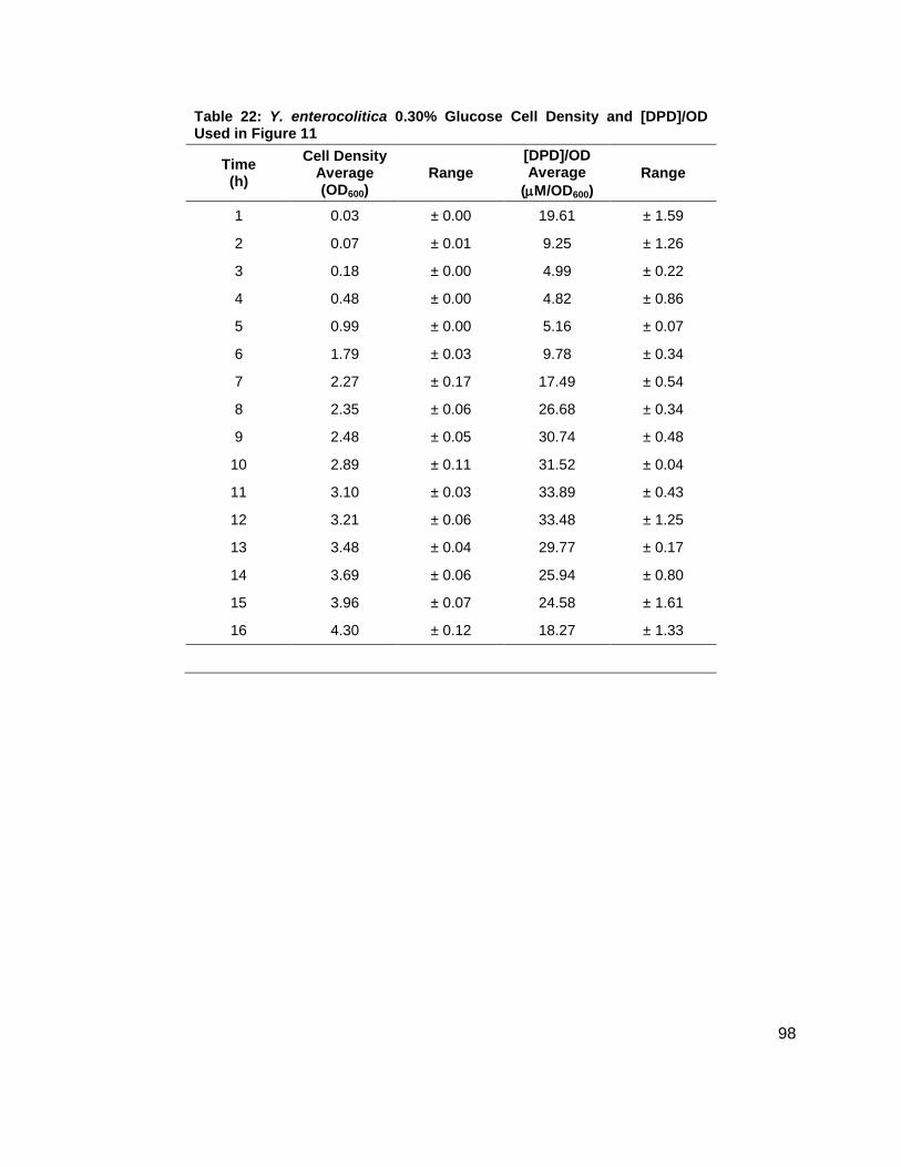
98


Time (h)


Range

[DPD]/OD Average

(M/OD600)

Range

1 0.03 ± 0.00 19.61 ± 1.59

2 0.07 ± 0.01 9.25 ± 1.26

3 0.18 ± 0.00 4.99 ± 0.22

4 0.48 ± 0.00 4.82 ± 0.86

5 0.99 ± 0.00 5.16 ± 0.07

6 1.79 ± 0.03 9.78 ± 0.34

7 2.27 ± 0.17 17.49 ± 0.54

8 2.35 ± 0.06 26.68 ± 0.34

9 2.48 ± 0.05 30.74 ± 0.48

10 2.89 ± 0.11 31.52 ± 0.04

11 3.10 ± 0.03 33.89 ± 0.43

12 3.21 ± 0.06 33.48 ± 1.25

13 3.48 ± 0.04 29.77 ± 0.17

14 3.69 ± 0.06 25.94 ± 0.80

15 3.96 ± 0.07 24.58 ± 1.61

16 4.30 ± 0.12 18.27 ± 1.33

99


Time (h)


Range

[DPD]/OD Average

(M/OD600)

Range

1 0.02 ± 0.00 21.41 ± 0.17

2 0.07 ± 0.01 8.84 ± 0.87

3 0.18 ± 0.00 4.89 ± 0.12

4 0.49 ± 0.00 3.96 ± 0.01

5 0.98 ± 0.00 5.58 ± 0.06

6 1.83 ± 0.03 10.33 ± 0.32

7 2.33 ± 0.01 17.64 ± 0.71

8 2.35 ± 0.02 26.04 ± 0.22

9 2.59 ± 0.02 29.33 ± 0.45

10 2.83 ± 0.05 33.39 ± 0.76

11 3.09 ± 0.04 32.82 ± 2.39

12 3.28 ± 0.02 34.26 ± 0.10

13 3.59 ± 0.02 30.18 ± 0.13

14 3.72 ± 0.05 33.29 ± 0.91

15 3.62 ± 0.22 34.40 ± 3.15

16 4.00 ± 0.02 27.45 ± 1.60

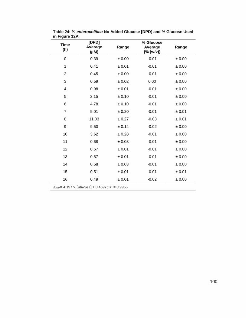
100

Table 24: Y. enterocolitica No Added Glucose [DPD] and % Glucose Used in Figure 12A

Time (h)

[DPD] Average

(M)

Range % Glucose

Average (% (w/v))

Range

0 0.39 ± 0.00 -0.01 ± 0.00

1 0.41 ± 0.01 -0.01 ± 0.00

2 0.45 ± 0.00 -0.01 ± 0.00

3 0.59 ± 0.02 0.00 ± 0.00

4 0.98 ± 0.01 -0.01 ± 0.00

5 2.15 ± 0.10 -0.01 ± 0.00

6 4.78 ± 0.10 -0.01 ± 0.00

7 9.01 ± 0.30 -0.01 ± 0.01

8 11.03 ± 0.27 -0.03 ± 0.01

9 9.50 ± 0.14 -0.02 ± 0.00

10 3.62 ± 0.28 -0.01 ± 0.00

11 0.68 ± 0.03 -0.01 ± 0.00

12 0.57 ± 0.01 -0.01 ± 0.00

13 0.57 ± 0.01 -0.01 ± 0.00

14 0.58 ± 0.03 -0.01 ± 0.00

15 0.51 ± 0.01 -0.01 ± 0.01

16 0.49 ± 0.01 -0.02 ± 0.00

A500 = 4.197 [ ] + 0.4597; R² = 0.9966

101

Table 25: Y. enterocolitica 0.08% Glucose [DPD] and % Glucose Used in Figure 12B

Time (h)

[DPD] Average

(M)

Range % Glucose

Average (% (w/v))

Range

0 0.34 ± 0.00 0.12 ± 0.01

1 0.40 ± 0.00 0.11 ± 0.03

2 0.47 ± 0.01 0.12 ± 0.03

3 0.62 ± 0.01 0.13 ± 0.03

4 1.04 ± 0.02 0.15 ± 0.01

5 2.74 ± 0.01 0.11 ± 0.01

6 7.72 ± 0.11 0.07 ± 0.00

7 19.14 ± 0.38 -0.01 ± 0.00

8 32.94 ± 0.45 -0.02 ± 0.00

9 50.34 ± 2.36 -0.02 ± 0.00

10 58.54 ± 0.46 -0.01 ± 0.01

11 43.39 ± 2.17 -0.01 ± 0.00

12 10.17 ± 5.03 -0.01 ± 0.00

13 0.73 ± 0.03 -0.01 ± 0.00

14 0.63 ± 0.02 -0.01 ± 0.00

15 0.52 ± 0.01 -0.01 ± 0.01

16 0.48 ± 0.02 -0.03 ± 0.00

A500 = 4.197 [ ] + 0.4597; R² = 0.9966

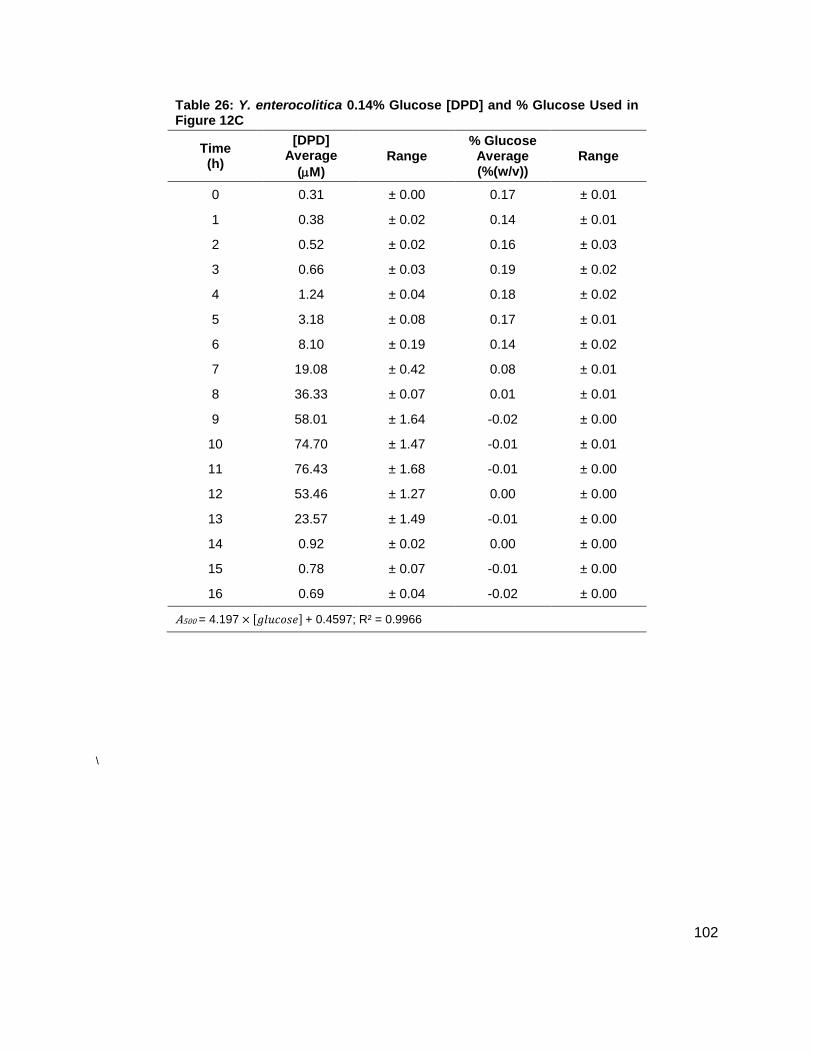
102

Table 26: Y. enterocolitica 0.14% Glucose [DPD] and % Glucose Used in Figure 12C

Time (h)

[DPD] Average

(M)

Range % Glucose

Average (%(w/v))

Range

0 0.31 ± 0.00 0.17 ± 0.01

1 0.38 ± 0.02 0.14 ± 0.01

2 0.52 ± 0.02 0.16 ± 0.03

3 0.66 ± 0.03 0.19 ± 0.02

4 1.24 ± 0.04 0.18 ± 0.02

5 3.18 ± 0.08 0.17 ± 0.01

6 8.10 ± 0.19 0.14 ± 0.02

7 19.08 ± 0.42 0.08 ± 0.01

8 36.33 ± 0.07 0.01 ± 0.01

9 58.01 ± 1.64 -0.02 ± 0.00

10 74.70 ± 1.47 -0.01 ± 0.01

11 76.43 ± 1.68 -0.01 ± 0.00

12 53.46 ± 1.27 0.00 ± 0.00

13 23.57 ± 1.49 -0.01 ± 0.00

14 0.92 ± 0.02 0.00 ± 0.00

15 0.78 ± 0.07 -0.01 ± 0.00

16 0.69 ± 0.04 -0.02 ± 0.00

A500 = 4.197 [ ] + 0.4597; R² = 0.9966

\

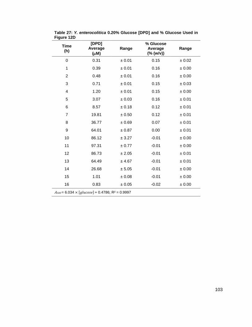
103

Table 27: Y. enterocolitica 0.20% Glucose [DPD] and % Glucose Used in Figure 12D

Time (h)

[DPD] Average

(M)

Range % Glucose

Average (% (w/v))

Range

0 0.31 ± 0.01 0.15 ± 0.02

1 0.39 ± 0.01 0.16 ± 0.00

2 0.48 ± 0.01 0.16 ± 0.00

3 0.71 ± 0.01 0.15 ± 0.03

4 1.20 ± 0.01 0.15 ± 0.00

5 3.07 ± 0.03 0.16 ± 0.01

6 8.57 ± 0.18 0.12 ± 0.01

7 19.81 ± 0.50 0.12 ± 0.01

8 36.77 ± 0.69 0.07 ± 0.01

9 64.01 ± 0.87 0.00 ± 0.01

10 86.12 ± 3.27 -0.01 ± 0.00

11 97.31 ± 0.77 -0.01 ± 0.00

12 86.73 ± 2.05 -0.01 ± 0.01

13 64.49 ± 4.67 -0.01 ± 0.01

14 26.68 ± 5.05 -0.01 ± 0.00

15 1.01 ± 0.08 -0.01 ± 0.00

16 0.83 ± 0.05 -0.02 ± 0.00

A500 = 6.034 [ ] + 0.4786; R² = 0.9997

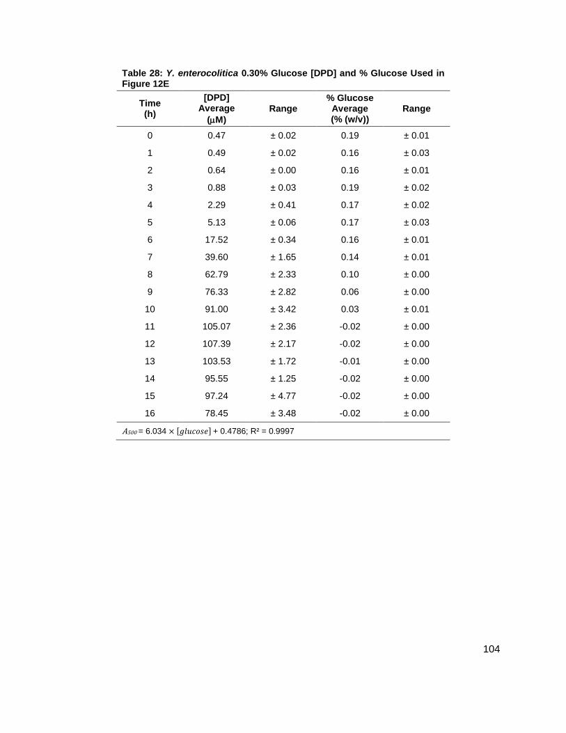
104

Table 28: Y. enterocolitica 0.30% Glucose [DPD] and % Glucose Used in Figure 12E

Time (h)

[DPD] Average

(M)

Range % Glucose

Average (% (w/v))

Range

0 0.47 ± 0.02 0.19 ± 0.01

1 0.49 ± 0.02 0.16 ± 0.03

2 0.64 ± 0.00 0.16 ± 0.01

3 0.88 ± 0.03 0.19 ± 0.02

4 2.29 ± 0.41 0.17 ± 0.02

5 5.13 ± 0.06 0.17 ± 0.03

6 17.52 ± 0.34 0.16 ± 0.01

7 39.60 ± 1.65 0.14 ± 0.01

8 62.79 ± 2.33 0.10 ± 0.00

9 76.33 ± 2.82 0.06 ± 0.00

10 91.00 ± 3.42 0.03 ± 0.01

11 105.07 ± 2.36 -0.02 ± 0.00

12 107.39 ± 2.17 -0.02 ± 0.00

13 103.53 ± 1.72 -0.01 ± 0.00

14 95.55 ± 1.25 -0.02 ± 0.00

15 97.24 ± 4.77 -0.02 ± 0.00

16 78.45 ± 3.48 -0.02 ± 0.00

A500 = 6.034 [ ] + 0.4786; R² = 0.9997

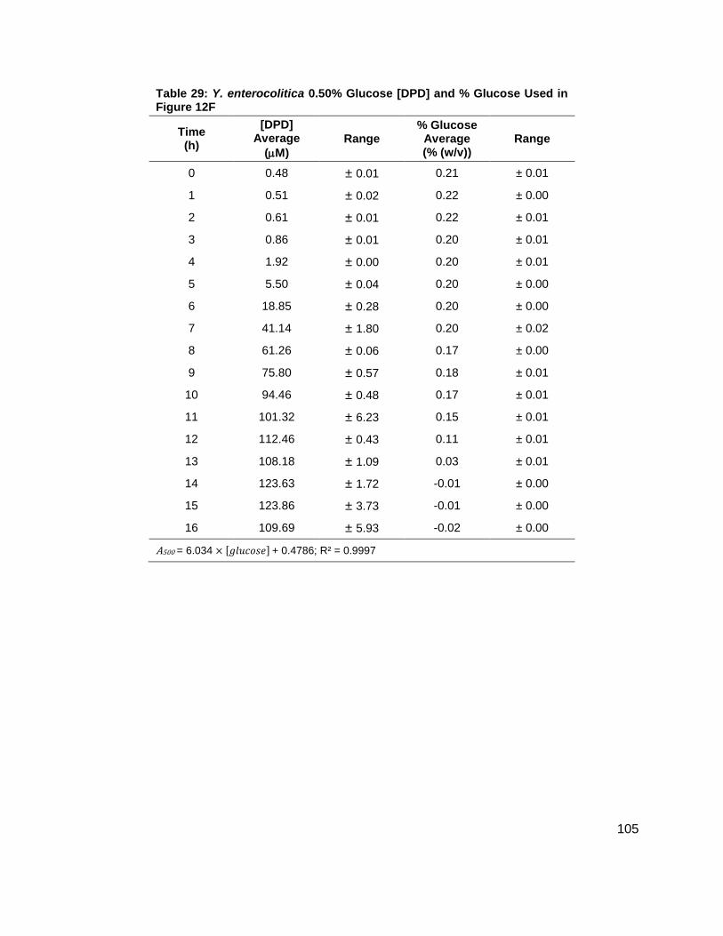
105

Table 29: Y. enterocolitica 0.50% Glucose [DPD] and % Glucose Used in Figure 12F

Time (h)

[DPD] Average

(M)

Range % Glucose

Average (% (w/v))

Range

0 0.48 ± 0.01 0.21 ± 0.01

1 0.51 ± 0.02 0.22 ± 0.00

2 0.61 ± 0.01 0.22 ± 0.01

3 0.86 ± 0.01 0.20 ± 0.01

4 1.92 ± 0.00 0.20 ± 0.01

5 5.50 ± 0.04 0.20 ± 0.00

6 18.85 ± 0.28 0.20 ± 0.00

7 41.14 ± 1.80 0.20 ± 0.02

8 61.26 ± 0.06 0.17 ± 0.00

9 75.80 ± 0.57 0.18 ± 0.01

10 94.46 ± 0.48 0.17 ± 0.01

11 101.32 ± 6.23 0.15 ± 0.01

12 112.46 ± 0.43 0.11 ± 0.01

13 108.18 ± 1.09 0.03 ± 0.01

14 123.63 ± 1.72 -0.01 ± 0.00

15 123.86 ± 3.73 -0.01 ± 0.00

16 109.69 ± 5.93 -0.02 ± 0.00

A500 = 6.034 [ ] + 0.4786; R² = 0.9997

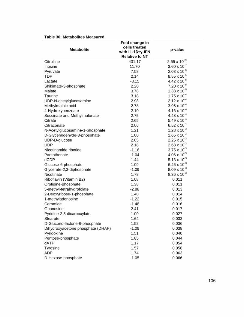
106

Table 30: Metabolites Measured

Metabolite

Fold change in cells treated

with IL-1β+γ-IFN Relative to NT

p-value

Citrulline 431.17 2.65 x 10-25

Inosine 11.70 3.60 x 10-7

Pyruvate 7.58 2.03 x 10-6

TDP 2.14 8.55 x 10-6

Lactate -8.15 4.42 x 10-5

Shikimate-3-phosphate 2.20 7.20 x 10-5

Malate 3.78 1.38 x 10-5

Taurine 3.18 1.75 x 10-4

UDP-N-acetylglucosamine 2.98 2.12 x 10-4

Methylmalnic acid 2.78 3.95 x 10-4

4-Hydroxybenzoate 2.10 4.16 x 10-4

Succinate and Methylmalonate 2.75 4.48 x 10-4

Citrate 2.65 5.49 x 10-4

Citraconate 2.06 6.52 x 10-4

N-Acetylglucosamine-1-phosphate 1.21 1.28 x 10-3

D-Glyceraldehyde-3-phosphate 1.00 1.65 x 10-3

UDP-D-glucose 2.05 2.25 x 10-3

UDP 2.18 2.68 x 10-3

Nicotinamide ribotide -1.16 3.75 x 10-3

Pantothenate -1.04 4.06 x 10-3

dCDP 1.44 5.13 x 10-3

Glucose-6-phosphate 1.09 6.46 x 10-3

Glycerate-2,3-diphosphate -1.09 8.09 x 10-3

Nicotinate 1.78 8.36 x 10-3

Riboflavin (Vitamin B2) 1.08 0.011

Orotidine-phosphate 1.38 0.011

5-methyl-tetrahydrofolate -2.88 0.013

2-Deoxyribose-1-phosphate 1.40 0.014

1-methyladenosine -1.22 0.015

Ceramide -1.48 0.016

Guanosine 2.41 0.017

Pyridine-2,3-dicarboxylate 1.00 0.027

Stearate 1.64 0.033

D-Glucono-lactone-6-phosphate 1.52 0.036

Dihydroxyacetone phosphate (DHAP) -1.09 0.038

Pyridoxine 1.51 0.040

Pentose-phosphate 1.85 0.044

dATP 1.17 0.054

Tyrosine 1.57 0.058

ADP 1.74 0.063

D-Hexose-phosphate -1.05 0.066

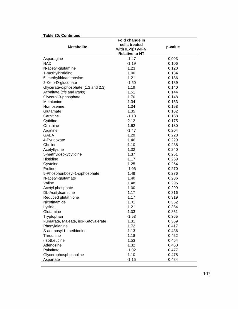
107

Table 30: Continued

Metabolite


with IL-1β+γ-IFN Relative to NT

p-value

Asparagine -1.47 0.093

NAD -1.19 0.106

N-acetyl-glutamine 1.23 0.120

1-methylhistidine 1.00 0.134

5'-methylthioadenosine 1.21 0.136

2-Keto-D-gluconate -1.50 0.139

Glycerate-diphosphate (1,3 and 2,3) 1.19 0.140

Aconitate (cis and trans) 1.51 0.144

Glycerol-3-phosphate 1.70 0.148

Methionine 1.34 0.153

Homoserine 1.34 0.158

Glutamate 1.35 0.162

Carnitine -1.13 0.168

Cytidine 2.12 0.175

Ornithine 1.62 0.180

Arginine -1.47 0.204

GABA 1.29 0.228

4-Pyridoxate 1.46 0.229

Choline 1.10 0.238

Acetyllysine 1.32 0.240

5-methyldeoxycytidine 1.37 0.251

Histidine 1.17 0.259

Cysteine 1.25 0.264

Proline -1.06 0.270

5-Phosphoribosyl-1-diphosphate 1.49 0.276

N-acetyl-glutamate 1.40 0.286

Valine 1.48 0.295

Acetyl phosphate 1.00 0.299

DL-Acetylcarnitine 1.17 0.316

Reduced glutathione 1.17 0.319

Nicotinamide 1.31 0.352

Lysine 1.21 0.354

Glutamine 1.03 0.361

Tryptophan -1.53 0.365

Fumarate, Maleate, iso-Ketovalerate 1.31 0.369

Phenylalanine 1.72 0.417

S-adenosyl-L-methionine 1.13 0.436

Threonine 1.18 0.452

(Iso)Leucine 1.53 0.454

Adenosine 1.32 0.460

Palmitate -1.92 0.477

Glycerophosphocholine 1.10 0.478

Aspartate -1.15 0.484

108

Table 31: Metabolites Measured

Metabolite


with Camptothecin Relative to NT

p-value

N-Acetylglucosamine-1-phosphate 3.79 1.79 x 10-5

Cysteine 3.59 1.83 x 10-5

1-methylhistidine 5.66 4.83 x 10-5

D-Glyceraldehyde-3-phosphate 1.50 5.23 x 10-5

Pantothenate 2.47 8.07 x 10-5

1-methyladenosine 4.83 8.41 x 10-5

Tryptophan 1.23 3.52 x 10-4

UDP-D-glucose 2.90 4.35 x 10-4

UDP-N-acetylglucosamine 3.10 4.99 x 10-4

Lactate 1.26 6.76 x 10-4

Methylmalnic acid 1.73 9.15 x 10-4

Succinate and Methylmalonate 1.72 1.09 x 10-3

5-methyldeoxycytidine 2.33 3.55 x 10-3

5-Phosphoribosyl-1-diphosphate -1.61 4.71 x 10-3

Nicotinamide ribotide -2.92 5.70 x 10-3

Shikimate-3-phosphate 1.60 6.36 x 10-3

D-Hexose-phosphate 1.79 7.37 x 10-3

Nicotinamide -1.04 7.53 x 10-3

2-Keto-D-gluconate -2.09 0.010

5'-methylthioadenosine 1.94 0.011

Glycerol-3-phosphate 2.64 0.012

Ornithine 2.20 0.012

Guanosine 3.02 0.013

Dihydroxyacetone phosphate (DHAP) 1.89 0.015

Pentose-phosphate 2.02 0.018

2-Deoxyribose-1-phosphate 1.43 0.019

N-acetyl-glutamate 1.59 0.020

Citrate 1.56 0.021

Lysine 3.16 0.022

Glutamine 2.65 0.023

ADP 3.92 0.028

Glycerate-2,3-diphosphate -1.06 0.032

Stearate -1.26 0.033

UDP 1.87 0.033

GABA 2.29 0.038

Riboflavin (Vitamin B2) 1.69 0.046

Taurine 2.37 0.048

Adenosine -1.44 0.049

Inosine 1.69 0.050

Orotidine-phosphate 1.12 0.050

Palmitate -1.08 0.053

Aspartate 1.64 0.062

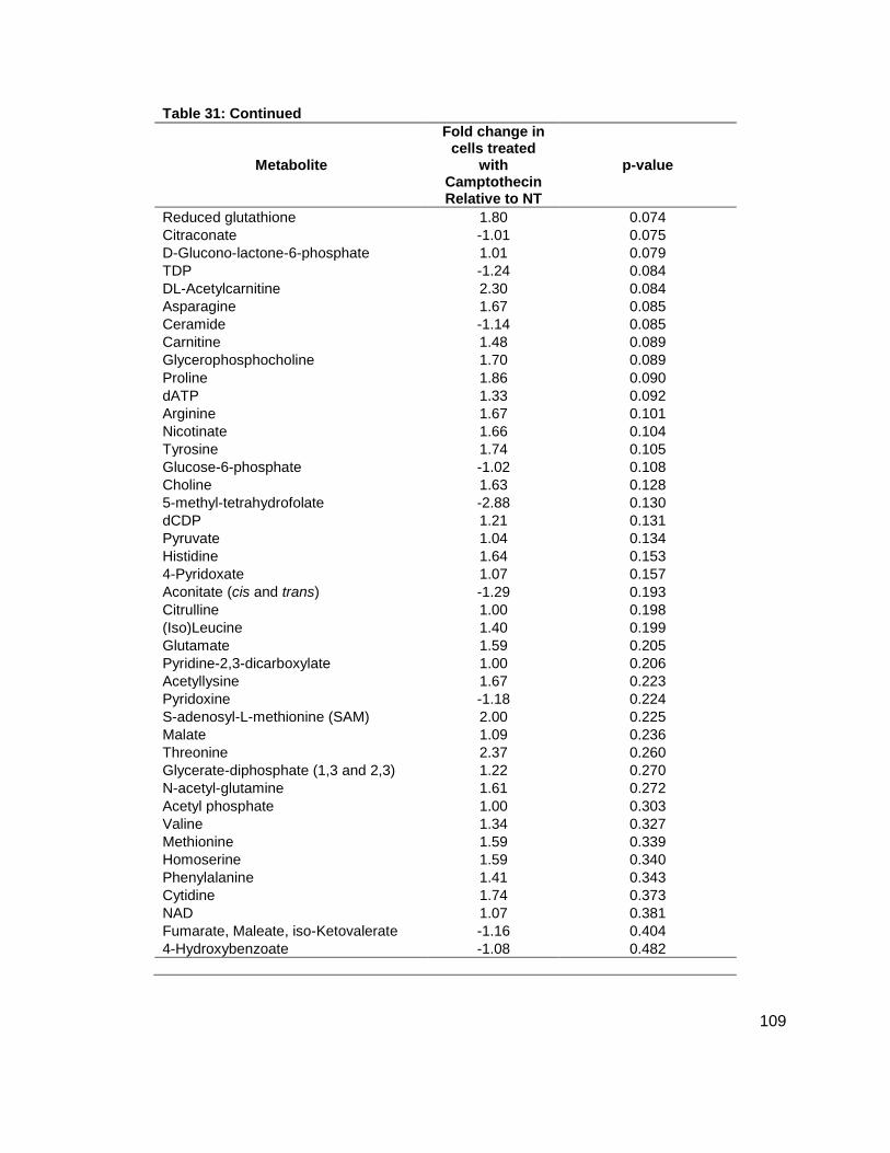
109

Table 31: Continued

Metabolite


with Camptothecin Relative to NT

p-value

Reduced glutathione 1.80 0.074

Citraconate -1.01 0.075

D-Glucono-lactone-6-phosphate 1.01 0.079

TDP -1.24 0.084

DL-Acetylcarnitine 2.30 0.084

Asparagine 1.67 0.085

Ceramide -1.14 0.085

Carnitine 1.48 0.089

Glycerophosphocholine 1.70 0.089

Proline 1.86 0.090

dATP 1.33 0.092

Arginine 1.67 0.101

Nicotinate 1.66 0.104

Tyrosine 1.74 0.105

Glucose-6-phosphate -1.02 0.108

Choline 1.63 0.128

5-methyl-tetrahydrofolate -2.88 0.130

dCDP 1.21 0.131

Pyruvate 1.04 0.134

Histidine 1.64 0.153

4-Pyridoxate 1.07 0.157

Aconitate (cis and trans) -1.29 0.193

Citrulline 1.00 0.198

(Iso)Leucine 1.40 0.199

Glutamate 1.59 0.205

Pyridine-2,3-dicarboxylate 1.00 0.206

Acetyllysine 1.67 0.223

Pyridoxine -1.18 0.224

S-adenosyl-L-methionine (SAM) 2.00 0.225

Malate 1.09 0.236

Threonine 2.37 0.260

Glycerate-diphosphate (1,3 and 2,3) 1.22 0.270

N-acetyl-glutamine 1.61 0.272

Acetyl phosphate 1.00 0.303

Valine 1.34 0.327

Methionine 1.59 0.339

Homoserine 1.59 0.340

Phenylalanine 1.41 0.343

Cytidine 1.74 0.373

NAD 1.07 0.381

Fumarate, Maleate, iso-Ketovalerate -1.16 0.404

4-Hydroxybenzoate -1.08 0.482

110

Vita

Mary Elizabeth Eisenhauer was born May 12, 1987 in Dayton, OH. After moving to Oak Ridge,

TN, she graduated from Oak Ridge High School in 2005. She attended Tennessee

Technological University where she received her Bachelor’s of Science in Chemistry in the

spring of 2009. At The University of Tennessee, Knoxville she began her graduate studies in

Chemistry, receiving her Master’s of Science in Chemistry in December 2011. Remaining at

UTK, she began graduate studies in the College of Education, and started teaching for Knox

County Schools in August 2011.

Documents

Application of Liquid Chromatography-Tandem Mass