Embed Size (px)
Citation preview

Application of Level Set Methods to Control & Reachability Problems
in Continuous & Hybrid Systems
Ian MitchellScientific Computing & Computational Mathematics Program
Stanford
5/17/02 2
Lots of Complex SystemsPhoto: Boeing
Photo: ActivMedia
Photo: IntelRequest 2 Grant 2
Request 1 Grant 1
asynchronous arbiter
automation interfaces
autonomous robots

5/17/02 3
Why Hybrid Systems?• Computers are increasingly interacting with external world
– Flexibility of such combinations yields huge design space– Design methods and tools targeted (mostly) at either continuous or
discrete systems• Example: aircraft flight control systems
seven mode collision avoidance protocol

5/17/02 4
Reachable Sets: What and Why?• One application: safety analysis
– What states are doomed to become unsafe?– What states are safe given an appropriate control strategy?
unsafe(a priori)
unsafe(uncontrollable) initial
conditions
safe (under appropriate control)
unsafe initialization

5/17/02 5
unsafe set with choiceto maneuver or not?
Seven Mode Safety Analysis
unsafe set with maneuver
unsafe set without maneuver
?unsafe
safe
5/17/02 6
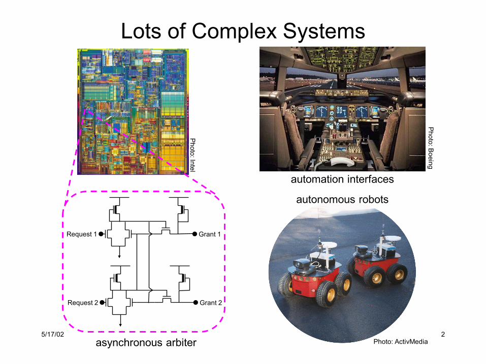
Seven Mode Safety Analysis• Ability to choose maneuver start time further reduces unsafe set
safe without switchunsafe to switch
safe with switch
unsafe with or without switch
[Tomlin, Mitchell & Ghosh, 2001]

5/17/02 7
My Contributions• Proved correctness of Hamilton-Jacobi-Isaacs
formulation for continuous backwards reachable sets• Implemented high resolution level set algorithms to
capitalize on this time dependent PDE formulation• Adapted projection concepts into HJI framework to
improve scalability• Demonstrated accurate computation of reachable
sets for nonlinear continuous and hybrid systems• Applied computed reachable sets to safety
verification, control synthesis and discrete abstraction problems in aircraft automation design

5/17/02 8
Outline• The discrete, the continuous and the somewhere in between
– Hybrid systems• What are reachable sets?
– Treating unknown inputs / parameters• Computing reachable sets for continuous systems
– A modified Hamilton-Jacobi-Isaacs equation– Application: synthesizing a safe control policy– Projective overapproximation of reachable sets
• Computing reachable sets for hybrid systems– The reach-avoid operator– Application: discrete abstraction– Application: an aircraft autolander
• Summary
5/17/02 9
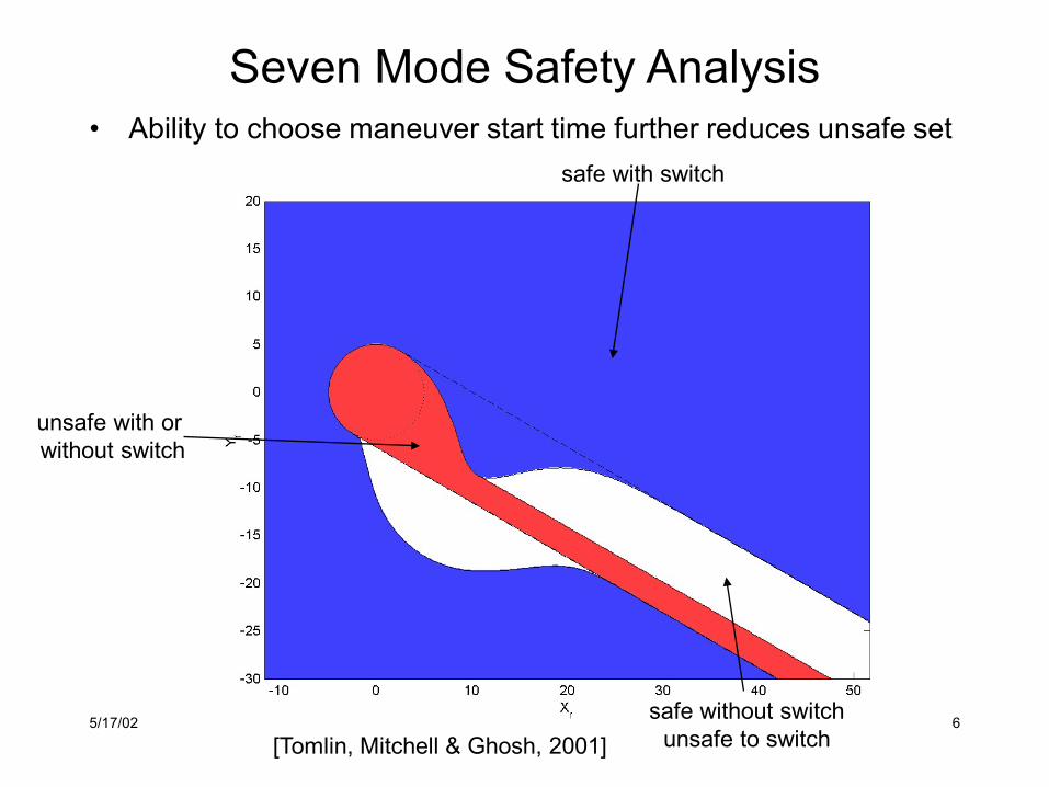
Finite Automata( )( ) ( ), ( )discrete states
( ) : discrete trajectrorydiscrete actions
( ) : action signal: transition function
i
i
Q
q t q t tq Q
q t Q
tQ
δ σ
σσδ
+ =
∈→
∈Σ→ Σ
×Σ →
1
2
σ1=cleared for takeoff
q1
taxi
q2
takeoffq3
climb
q4
cruise
q5
descendq6
land
reached cruise altitudeairborne
σ2=new altitude is clearσ3=cleared for landing
on the ground
5/17/02 10
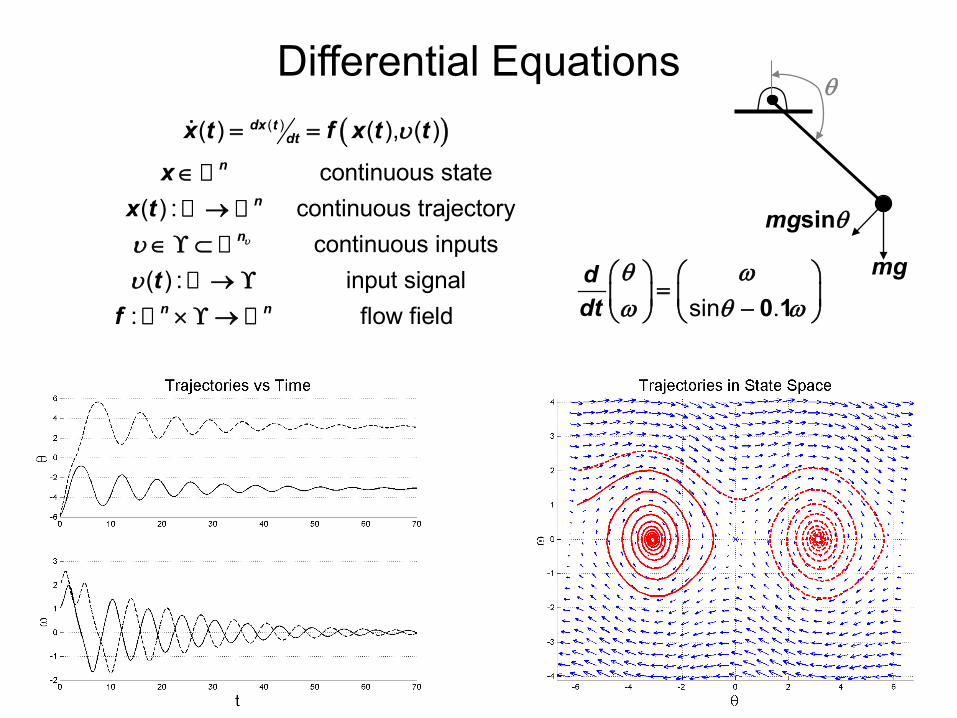
Differential Equations( )( )( ) ( ), ( )
continuous state( ) : continuous trajectory
continuous inputs( ) : input signal
: flow field
dx tdt
n
n
n
n n
x t f x t t
xx t
tf
υ
υ
υυ
= =
∈→
∈ϒ ⊂→ ϒ
× ϒ →
sin .ddt
θ ωω θ ω
= − 0 1
θ
mg
mgsinθ

5/17/02 11
Hybrid Automata• Discrete modes and
transitions• Continuous evolution within
each mode
σ1 = initiate maneuver t = π/4
q1
straight1( , )Sx f x υ=
q2
arc1( , )Ax f x υ=
q7
straight4( , )Sx f x υ=
q5
straight3( , )Sx f x υ=
q3
straight2( , )Sx f x υ=
q4
arc2( , )Ax f x υ=
q6
arc3( , )Ax f x υ=
t = T
t = π/4
t = π/2
t = T
cossin
dynamics in straight modes
Sx v v
fx v
ψψ
− + =
1
2
cossin
dynamics in arc modes
Ax v v x
fx v x
ψψ
− + − = +
1 2
2 1
5/17/02 12
Outline• The discrete, the continuous and the somewhere in between
– Hybrid systems• What are reachable sets?
– Treating unknown inputs / parameters• Computing reachable sets for continuous systems
– A modified Hamilton-Jacobi-Isaacs equation– Application: synthesizing a safe control policy– Projective overapproximation of reachable sets
• Computing reachable sets for hybrid systems– The reach-avoid operator– Application: discrete abstraction– Application: an aircraft autolander
• Summary

5/17/02 13
Discrete Backward Reachable Sets• Set of all states from which trajectories can reach some given
target state– For example: from what states can we reach “cruise”?
( )q t q t tδ σ+ =( 1) ( ), ( )
σ1=cleared for takeoff
q1
taxi
q2
takeoffq3
climb
q4
cruise
q5
descendq6
land
reached cruise altitudeairborne
σ2=new altitude is clearσ3=cleared for landing
Discrete System Dynamics
5/17/02 14
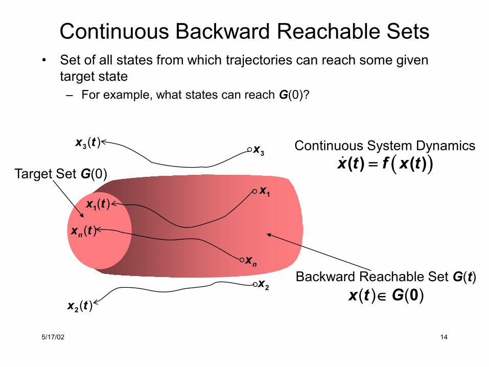
Backward Reachable Set G(t)( ) ( )x t G∈ 0
Continuous Backward Reachable Sets• Set of all states from which trajectories can reach some given
target state– For example, what states can reach G(0)?
Target Set G(0)
( )x t1
x1
x3( )x t3
nx
( )nx t
x2
( )x t2
( )x t f x t=( ) ( )Continuous System Dynamics
5/17/02 15
G(t3)G(t2)G(t1)
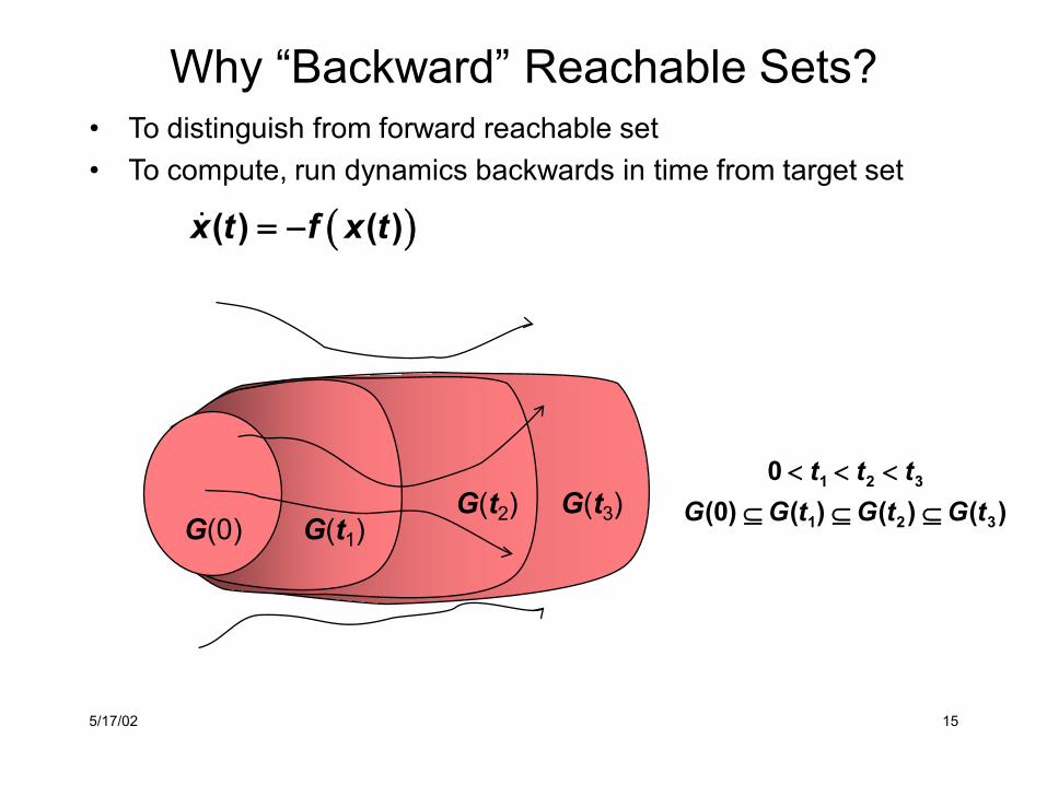
Why “Backward” Reachable Sets?• To distinguish from forward reachable set• To compute, run dynamics backwards in time from target set
G(0)
( )x t f x t= −( ) ( )
t t tG G t G t G t
< < <⊆ ⊆ ⊆
1 2 3
1 2 3
0(0) ( ) ( ) ( )
5/17/02 16
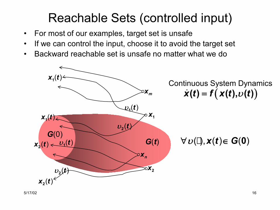
G(t) ( ), ( ) ( )x t Gυ∀ ∈ 0
Reachable Sets (controlled input)• For most of our examples, target set is unsafe• If we can control the input, choose it to avoid the target set• Backward reachable set is unsafe no matter what we do
G(0)
nx
mx
x1
( )x t1
( )tυ1
( )x t1
( )tυ2
x2
( )tυ1( )x t2
( )x t2
( )tυ2
( )x t f x t tυ=( ) ( ), ( )Continuous System Dynamics

5/17/02 17
G(t)
Reachable Sets (uncontrolled input)• Sometimes we have no control over input signal
– noise, actions of other agents, unknown system parameters• It is safest to assume the worst case
( )x t1x1
( )x t1
x2
( )x t2
nx
mx
( ), ( ) ( )x t Gυ∃ ∈ 0
( )x t f x t tυ=( ) ( ), ( )Continuous System Dynamics
( )x t2
G(0)
( )tυ1
( )tυ2
( )tυ1
( )tυ2
5/17/02 18
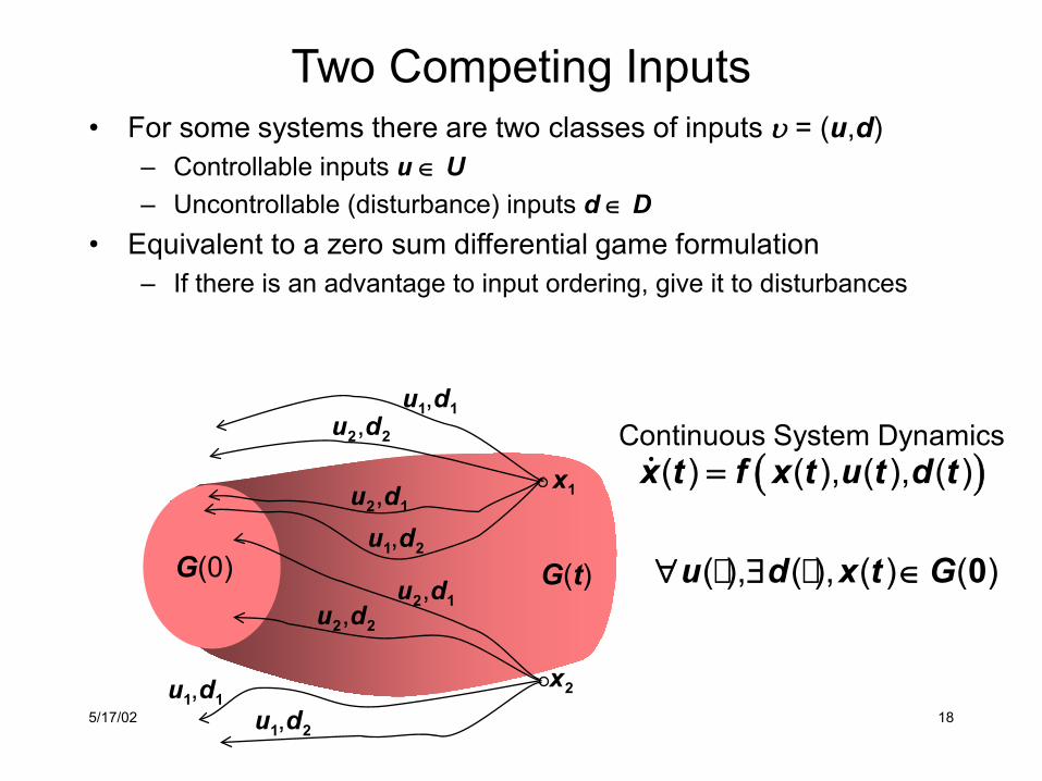
( ), ( ), ( ) ( )u d x t G∀ ∃ ∈ 0
Two Competing Inputs• For some systems there are two classes of inputs υ = (u,d)
– Controllable inputs u ∈ U– Uncontrollable (disturbance) inputs d ∈ D
• Equivalent to a zero sum differential game formulation– If there is an advantage to input ordering, give it to disturbances
( )( ) ( ), ( ), ( )x t f x t u t d t=
G(0)
x1
x2,u d1 1
,u d1 2
,u d2 2
,u d2 1
,u d1 1
,u d1 2
,u d2 1,u d2 2
Continuous System Dynamics
G(t)
5/17/02 19
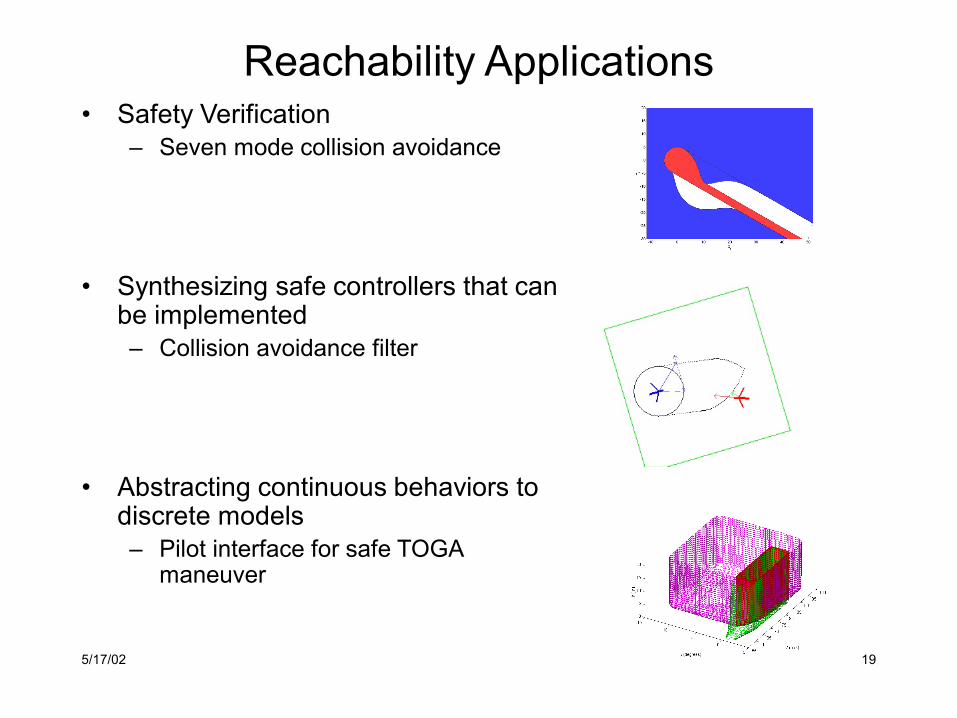
Reachability Applications• Safety Verification
– Seven mode collision avoidance
• Synthesizing safe controllers that can be implemented– Collision avoidance filter
• Abstracting continuous behaviors to discrete models– Pilot interface for safe TOGA
maneuver
5/17/02 20
Outline• The discrete, the continuous and the somewhere in between
– Hybrid systems• What are reachable sets?
– Treating unknown inputs / parameters• Computing reachable sets for continuous systems
– A modified Hamilton-Jacobi-Isaacs equation– Application: synthesizing a safe control policy– Projective overapproximation of reachable sets
• Computing reachable sets for hybrid systems– The reach-avoid operator– Application: discrete abstraction– Application: an aircraft autolander
• Summary

5/17/02 21
Computing Continuous Reachable Sets• Two key questions:
– How to represent continuous sets?– How to evolve sets according to system dynamics?
• Two philosophies:– Forwards reachable set computed by following system trajectories– Backwards reachable set computed on a motionless grid
• My method (based on level set algorithms)– Backwards reachable set on a fixed grid– Implicit surface representation of sets– Solve Hamilton-Jacobi equation to evolve sets

5/17/02 22
Forward Reachability• Forwards reachable set is computed by following trajectories• Examples:
– Timed automata: Uppaal [Larsen, Pettersson…], Kronos [Yovine,…], …
– Rectangular differential inclusions: Hytech, Hypertech [Henzinger, Ho, Horowitz, Wong-Toi, …]
– Polyhedra and linear dynamics: Checkmate [Chutinan & Krogh], d/dt [Bournez, Dang, Maler, Pnueli, …], others [Bemporad, Morari, Torrisi, …], [Greenstreet & Mitchell], …
– Ellipsoids and linear dynamics [Botchkarev, Kurzhanski, Tripakis, Varaiya, …]
– Discretization (predicate abstraction) on grid [Kurshan & McMillan] or by cylindrical algebraic decomposition [Tiwari & Khanna]
• Advantages: Compact representation of sets, overapproximation guarantees
• Disadvantages: Linear dynamics, reliance on trajectory optimization, restrictive set representation, potentially large error
5/17/02 23
Backwards Reachability• Backwards reachable set is computed on a motionless grid• Examples:
– Time dependent Hamilton-Jacobi [Sastry, Lygeros, Tomlin, …]– Static Hamilton-Jacobi [Bardi, Capuzzo-Dolcetta, Falcone, …]– Viability theory [Aubin, Quincampoix, Saint-Pierre, …]
• Advantages: General representation of sets, nonlinear dynamics• Disadvantages: Exponential growth of representation size with
state dimension, direction of error is unknown
5/17/02 24
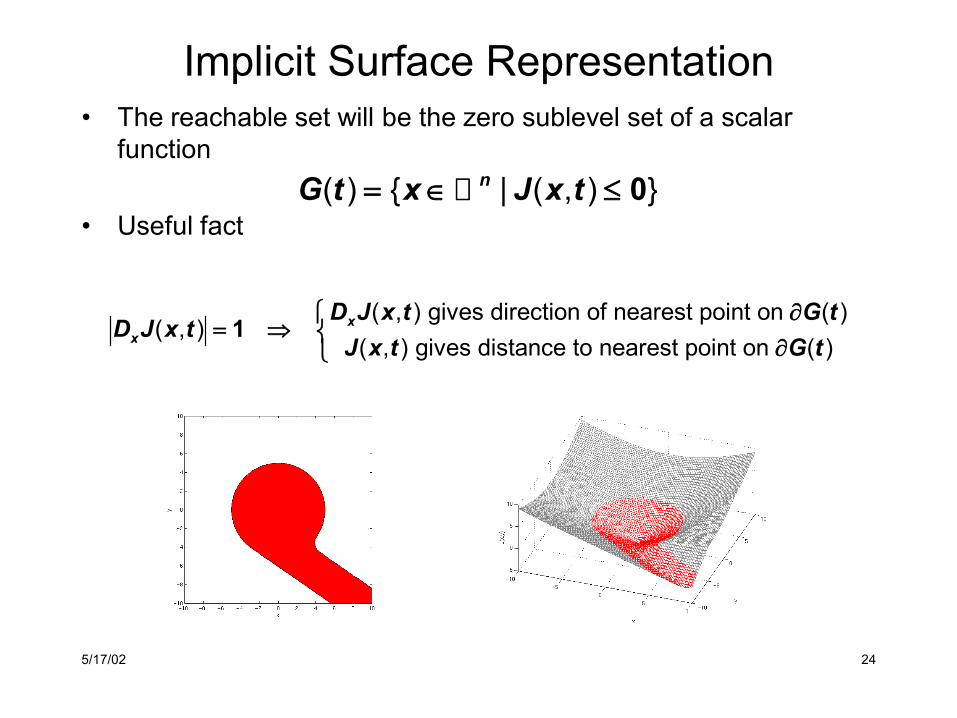
Implicit Surface Representation• The reachable set will be the zero sublevel set of a scalar
function
• Useful fact
( , ) gives direction of nearest point on ( )( , )
( , ) gives distance to nearest point on ( )x
xD J x t G t
D J x tJ x t G t
∂= ⇒ ∂
1
( ) { | ( , ) }nG t x J x t= ∈ ≤ 0
5/17/02 25
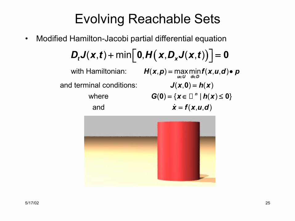
Evolving Reachable Sets• Modified Hamilton-Jacobi partial differential equation
( )( , ) min , , ( , )t xD J x t H x D J x t + = 0 0with Hamiltonian: ( , ) maxmin ( , , )
and terminal conditions: ( , ) ( )where ( ) { | ( ) }and ( , , )
d Du U
n
H x p f x u d p
J x h xG x h x
x f x u d
∈∈= •
== ∈ ≤
=
00 0
5/17/02 26
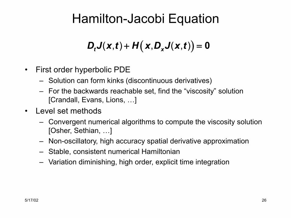
Hamilton-Jacobi Equation
• First order hyperbolic PDE– Solution can form kinks (discontinuous derivatives)– For the backwards reachable set, find the “viscosity” solution
[Crandall, Evans, Lions, …]• Level set methods
– Convergent numerical algorithms to compute the viscosity solution [Osher, Sethian, …]
– Non-oscillatory, high accuracy spatial derivative approximation– Stable, consistent numerical Hamiltonian– Variation diminishing, high order, explicit time integration
( )( , ) , ( , )t xD J x t H x D J x t+ = 0
5/17/02 27
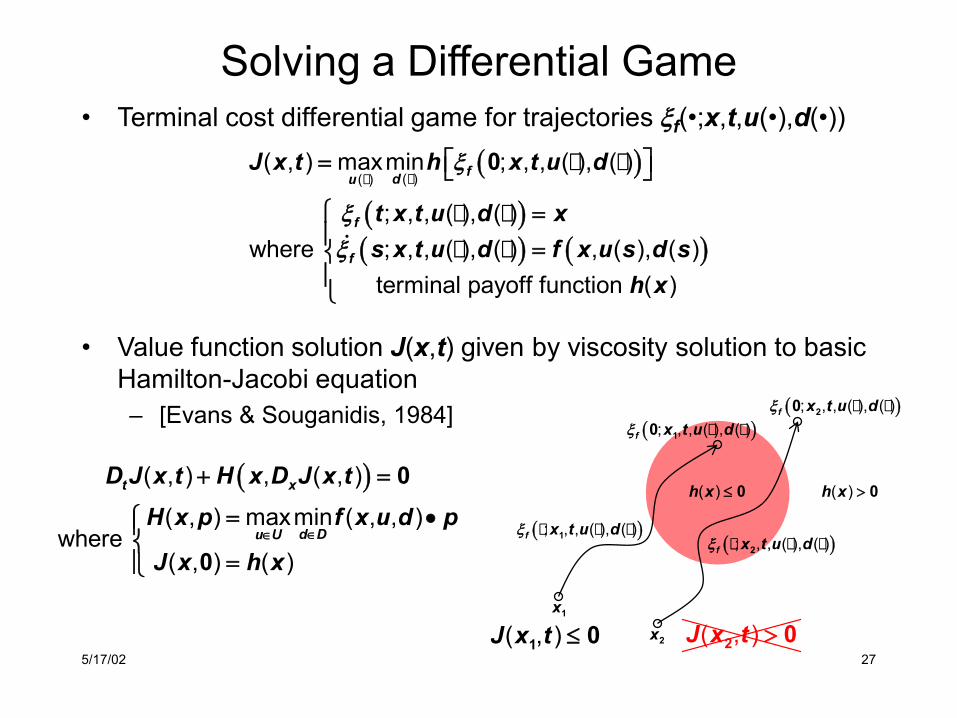
Solving a Differential Game• Terminal cost differential game for trajectories ξf(•;x,t,u(•),d(•))
• Value function solution J(x,t) given by viscosity solution to basic Hamilton-Jacobi equation– [Evans & Souganidis, 1984]
( )
( )( ) ( )
( )( )( , ) maxmin ; , , ( ), ( )
; , , ( ), ( )where ; , , ( ), ( ) , ( ), ( )
terminal payoff function ( )
fdu
f
f
J x t h x t u d
t x t u d xs x t u d f x u s d s
h x
ξ
ξξ
=
= =
0
( )( , ) , ( , )
( , ) maxmin ( , , )where
( , ) ( )
t x
d Du U
D J x t H x D J x tH x p f x u d p
J x h x∈∈
+ =
= •
=
0
0
( ); , , ( ), ( )f x t u dξ 10
( ); , , ( ), ( )f x t u dξ 2
x1
( ); , , ( ), ( )f x t u dξ 1
( ); , , ( ), ( )f x t u dξ 20
( )h x ≤ 0 ( )h x > 0
x2( , )J x t ≤1 0 ( , )J x t >2 0

5/17/02 28
Modification for Optimal Stopping Time• How to keep trajectories from passing through G(0)?
– [Mitchell, Bayen & Tomlin 2002]– Augment disturbance input
– Augmented Hamilton-Jacobi equation solves for reachable set
– Augmented Hamiltonian is equivalent to modified Hamiltonian
( )( , ) maxmin ( , , )
( , ) , ( , ) where ( , ) ( )
u U d Dt x
H x p f x u d pD J x t H x D J x t
J x h x∈ ∈
= •+ = =
00
[ ] [ ] [ ] where : , ,
( , , ) ( , , )
d d d d t
f x u d d f x u d
= →
=
0 0 1
[ ][ , ]
( , ) maxmin ( , , )
maxmin min ( , , )
min ,maxmin ( , , ) min , ( , )
u U d D
d D du U
d Du U
H x p f x u d p
d f x u d p
f x u d p H x p
∈ ∈
∈ ∈∈
∈∈
= •
= •
= • =
0 1
0 0
( ); , , ( ), ( )f x t u dξ 2
( ); , , ( ), ( )f x t u dξ 20
x2
( , )J x t ≤2 0
5/17/02 29
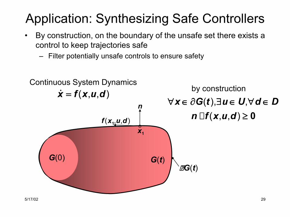
Application: Synthesizing Safe Controllers• By construction, on the boundary of the unsafe set there exists a
control to keep trajectories safe– Filter potentially unsafe controls to ensure safety
( , , )x f x u d=Continuous System Dynamics
( , , )f x u d1
n
x1
( ), ,( , , )
x G t u U d Dn f x u d
∀ ∈∂ ∃ ∈ ∀ ∈≥ 0
by construction
G(0) G(t)G(t)
5/17/02 30
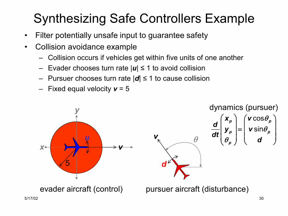
Synthesizing Safe Controllers Example• Filter potentially unsafe input to guarantee safety• Collision avoidance example
– Collision occurs if vehicles get within five units of one another– Evader chooses turn rate |u| ≤ 1 to avoid collision– Pursuer chooses turn rate |d| ≤ 1 to cause collision– Fixed equal velocity v = 5
evader aircraft (control) pursuer aircraft (disturbance)
y
5
xu
vθ
d
v
cossin
p p
p p
p
x vd y vdt
d
θθ
θ
=
dynamics (pursuer)
5/17/02 31
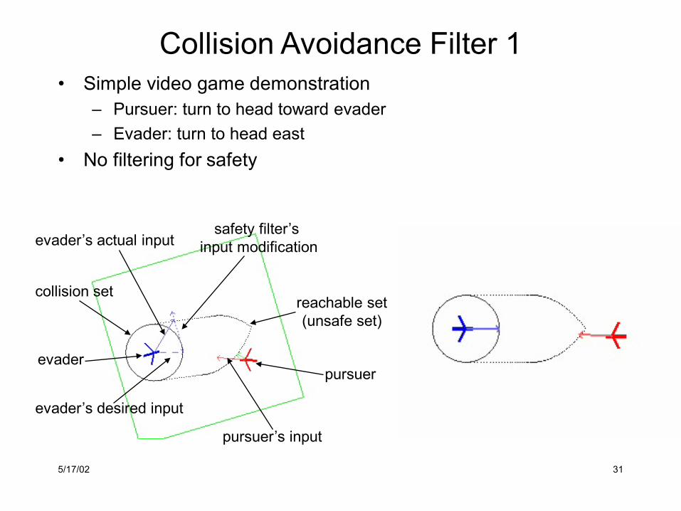
Collision Avoidance Filter 1• Simple video game demonstration
– Pursuer: turn to head toward evader– Evader: turn to head east
• No filtering for safety
pursuer
safety filter’s input modification
pursuer’s input
evader’s desired input
evader
evader’s actual input
reachable set(unsafe set)
collision set
5/17/02 32
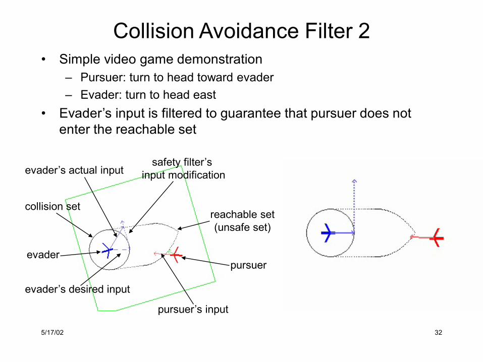
Collision Avoidance Filter 2• Simple video game demonstration
– Pursuer: turn to head toward evader– Evader: turn to head east
• Evader’s input is filtered to guarantee that pursuer does not enter the reachable set
pursuer
safety filter’s input modification
pursuer’s input
evader’s desired input
evader
evader’s actual input
reachable set(unsafe set)
collision set

5/17/02 33
Collision Avoidance Filter 3• Simple video game demonstration
– Pursuer: turn to head toward evader– Evader: turn to head east
• Evader’s input is filtered, but pursuer is already inside reachable set, so collision cannot be avoided
pursuer
safety filter’s input modification
pursuer’s input
evader’s desired input
evader
evader’s actual input
reachable set(unsafe set)
collision set

5/17/02 34
Collision Avoidance Computation• Work in relative coordinates with evader fixed at origin
– State variables are now relative planar location (x,y) and relative heading ψ
cossin
x v v uyd y v uxdt
d u
ψψ
ψ
− + + = − −
evader aircraft (control) pursuer aircraft (disturbance)
x
y
uv
ψ
d
v

5/17/02 35
Hamilton-Jacobi Formulation• Evader tries to maintain five mile separation
( , )( , ) cos sin ( ) ( )
cos sin | | | |x x y x y
x x y x y
J x t x yH x p p v p v p v u p y p x p d p
p v p v p v p y p x p pψ ψ
ψ ψ
ψ ψ
ψ ψ
= = + −
= + + + − − −
= + + + − − −
2 20 5
unsafe set (at any ψ)
5x
y
let: ( , ), ,xp D J x t u d= ≤ ≤1 1

5/17/02 36
Computing Reachable Set
rendering software by Prof. Ron Fedkiw
ψ
x
y( ){ }
solve: ( , ) min , , ( , )
display: ( ) | ( , )t x
n
D J x t H x D J x t
G t x J x t
+ =
= ∈ ≤
0 0
0
5/17/02 37
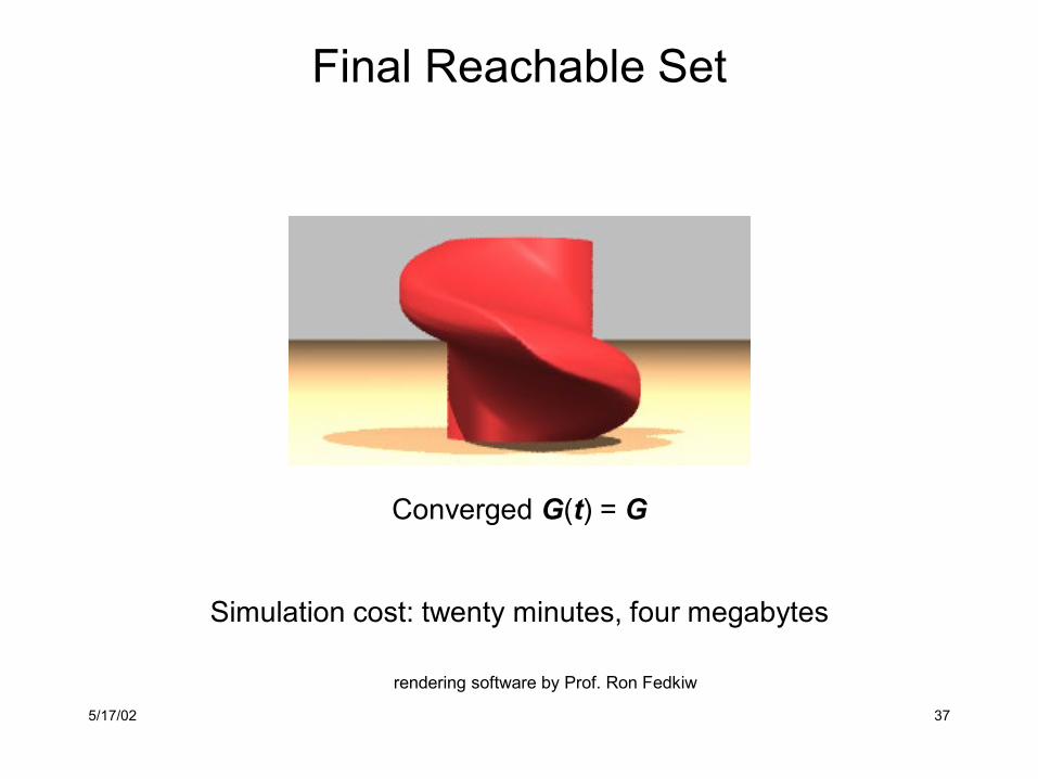
Final Reachable Set
Simulation cost: twenty minutes, four megabytes
Converged G(t) = G
rendering software by Prof. Ron Fedkiw
5/17/02 38
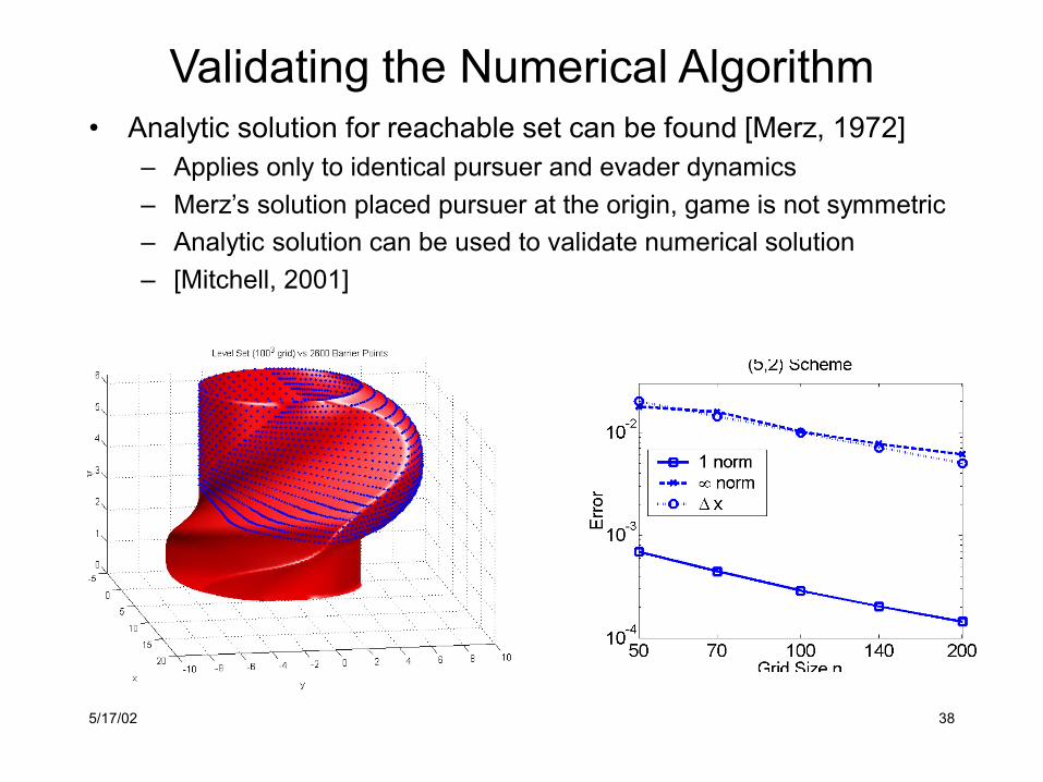
Validating the Numerical Algorithm• Analytic solution for reachable set can be found [Merz, 1972]
– Applies only to identical pursuer and evader dynamics– Merz’s solution placed pursuer at the origin, game is not symmetric– Analytic solution can be used to validate numerical solution– [Mitchell, 2001]

5/17/02 39
Innovation in Level Set Methods• Level set methods are prone to area/volume loss
– Particle level set method is an easy to program technique that significantly improves volume preservation
– [Enright, Fedkiw, Ferziger & Mitchell, 2002]Level Set Only Particle Level Set
Rendering by Sou Cheng Choi
5/17/02 40
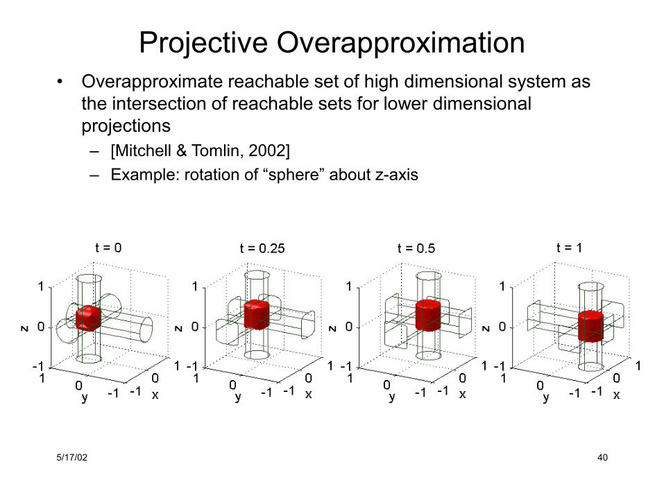
Projective Overapproximation• Overapproximate reachable set of high dimensional system as
the intersection of reachable sets for lower dimensional projections– [Mitchell & Tomlin, 2002]– Example: rotation of “sphere” about z-axis
5/17/02 41
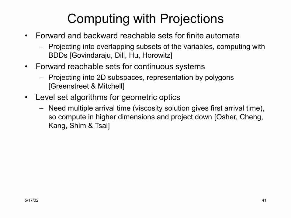
Computing with Projections• Forward and backward reachable sets for finite automata
– Projecting into overlapping subsets of the variables, computing with BDDs [Govindaraju, Dill, Hu, Horowitz]
• Forward reachable sets for continuous systems– Projecting into 2D subspaces, representation by polygons
[Greenstreet & Mitchell]• Level set algorithms for geometric optics
– Need multiple arrival time (viscosity solution gives first arrival time), so compute in higher dimensions and project down [Osher, Cheng, Kang, Shim & Tsai]

5/17/02 42
Hamilton-Jacobi in the Projection• Consider x-z projection represented by level set Jxz(x,z,t)
– Back projection into 3D yields a cylinder Jxz(x,y,z,t)• Simple HJ PDE for this cylinder
– But for cylinder parallel to y-axis, p2 = 0
• What value to give free variable y in fi(x,y,z)?– Treat it as a disturbance, bounded by the other projections
• Hamiltonian no longer depends on y, so computation can be done entirely in x-z space on Jxz(x,z,t)
( , , , ) ( , , )t xz i ii
D J x y z t p f x y z=
+ =∑3
10
( , , , )where ( , , , )
( , , , )
x xz
y xz
z xz
p D J x y z tp D J x y z tp D J x y z t
= = =
1
2
3
( , , , ) ( , , ) ( , , )t xzD J x y z t p f x y z p f x y z+ + =1 1 3 3 0
[ ]( , , , ) min ( , , ) ( , , )t xz yD J x y z t p f x y z p f x y z+ + =1 1 3 3 0

5/17/02 43
Projective Collision Avoidance• Work strictly in relative x-y plane
– Treat relative heading ψ ∈ [ 0, 2π ] as a disturbance input– Compute time: 40 seconds in 2D vs 20 minutes in 3D– Compare overapproximative prism (mesh) to true set (solid)
5/17/02 44
Outline• The discrete, the continuous and the somewhere in between
– Hybrid systems• What are reachable sets?
– Treating unknown inputs / parameters• Computing reachable sets for continuous systems
– A modified Hamilton-Jacobi-Isaacs equation– Application: synthesizing a safe control policy– Projective overapproximation of reachable sets
• Computing reachable sets for hybrid systems– The reach-avoid operator– Application: discrete abstraction– Application: an aircraft autolander
• Summary
5/17/02 45
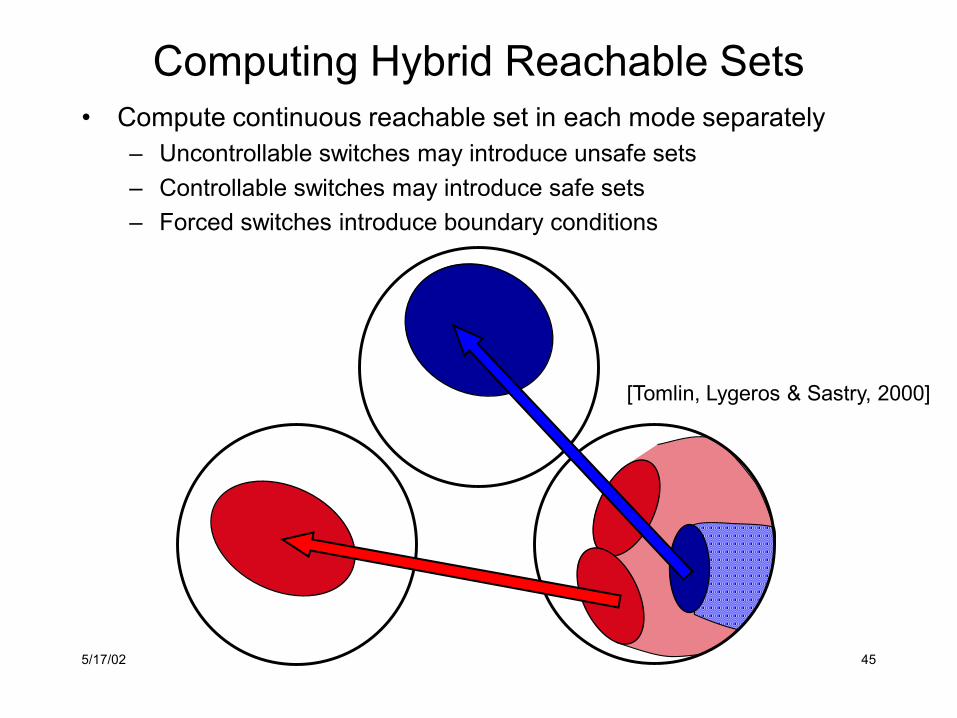
Computing Hybrid Reachable Sets• Compute continuous reachable set in each mode separately
– Uncontrollable switches may introduce unsafe sets– Controllable switches may introduce safe sets– Forced switches introduce boundary conditions
[Tomlin, Lygeros & Sastry, 2000]
5/17/02 46
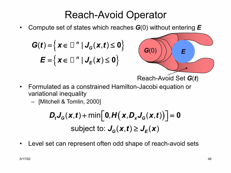
• Compute set of states which reaches G(0) without entering E
• Formulated as a constrained Hamilton-Jacobi equation or variational inequality– [Mitchell & Tomlin, 2000]
• Level set can represent often odd shape of reach-avoid sets
Reach-Avoid Operator
{ }{ }
( ) | ( , )
| ( )
nG
nE
G t x J x t
E x J x
= ∈ ≤
= ∈ ≤
0
0
( )( , ) min , , ( , )
subject to: ( , ) ( )t G x G
G E
D J x t H x D J x tJ x t J x
+ = ≥
0 0
G(0) E
Reach-Avoid Set G(t)
5/17/02 47
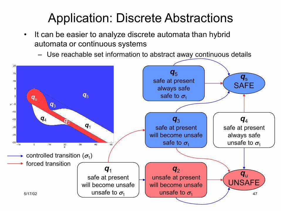
Application: Discrete Abstractions• It can be easier to analyze discrete automata than hybrid
automata or continuous systems– Use reachable set information to abstract away continuous details
q1safe at present
will become unsafeunsafe to σ1
q5safe at present
always safesafe to σ1
q3safe at present
will become unsafesafe to σ1
q4safe at present
always safeunsafe to σ1
q2unsafe at present
will become unsafeunsafe to σ1
qsSAFE
quUNSAFE
forced transitioncontrolled transition (σ1)
q1
q5
q3
qu
q4 q2

5/17/02 48
Application: Aircraft Autolander• Airplane must stay within safe flight envelope during landing
– Bounds on velocity (V), flight path angle (γ), height (z)– Control over engine thrust (T), angle of attack (α), flap settings– Model flap settings as discrete modes of hybrid automata– Terms in continuous dynamics may depend on flap setting– [Mitchell, Bayen & Tomlin, 2001]
γα
VT
D
L
mg
inertial frame
wind frame
body frame
z
[ cos , sin ]( ) [ sin , cos ]
sin
( )( )
m V mgd m V mgd
VV
z Vt
TDTL
α αα
γαγ γγ
−
−
− − = + −
1
1

5/17/02 49
Landing Example: Discrete Model• Flap dynamics version
– Pilot can choose one of three flap deflections
– Thirty seconds for zero to full deflection
• Implemented version– Instant switches between
fixed deflections– Additional timed modes to
remove Zeno behavior
retract
0u 25d 50d
deflect
0u
25d
50d
0t
25t
50t
controlledforcedinitial
5/17/02 50
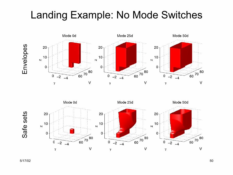
Landing Example: No Mode SwitchesEn
velo
pes
Safe
set
s
5/17/02 51
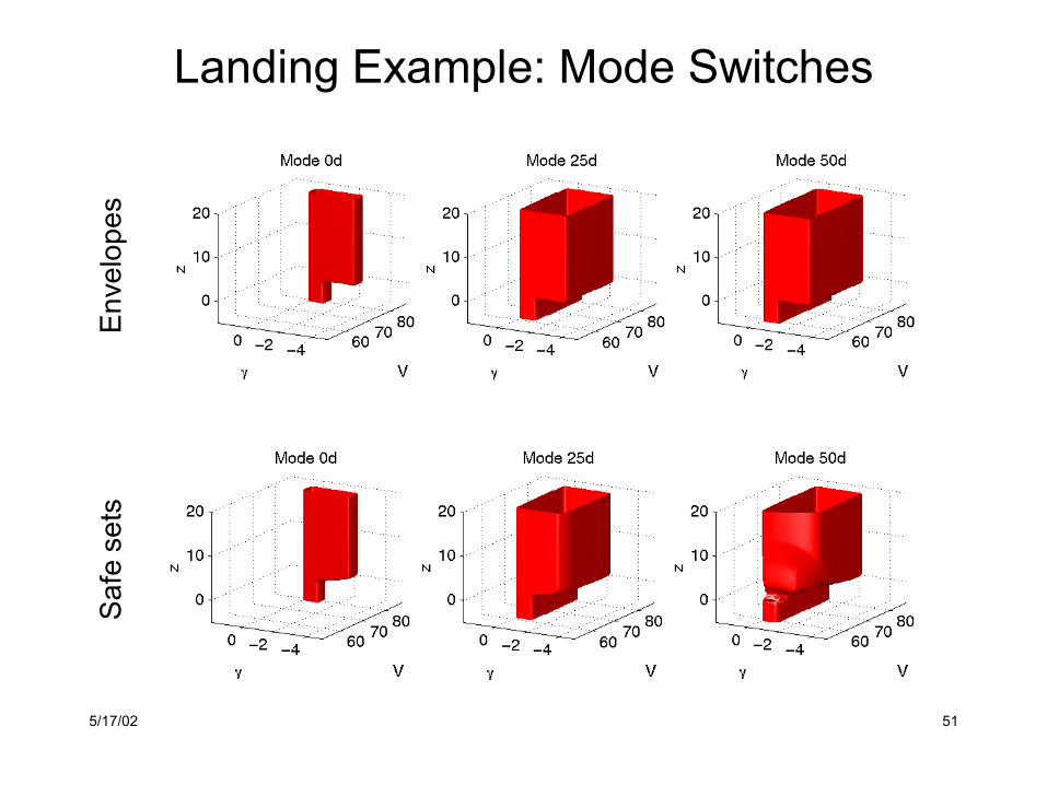
Landing Example: Mode SwitchesEn
velo
pes
Safe
set
s
5/17/02 52
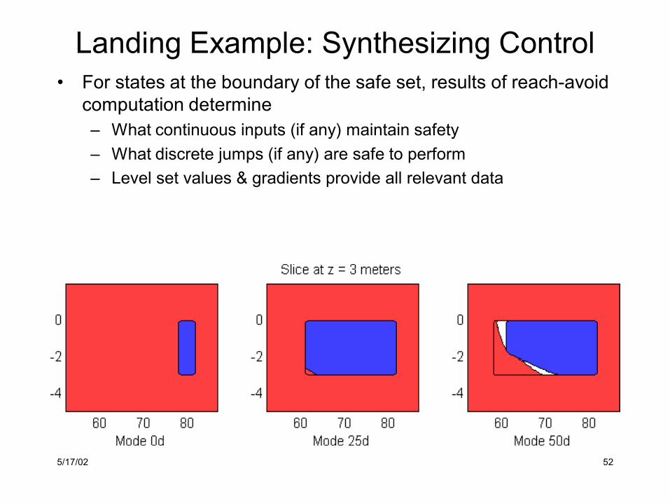
Landing Example: Synthesizing Control• For states at the boundary of the safe set, results of reach-avoid
computation determine– What continuous inputs (if any) maintain safety– What discrete jumps (if any) are safe to perform– Level set values & gradients provide all relevant data
5/17/02 53
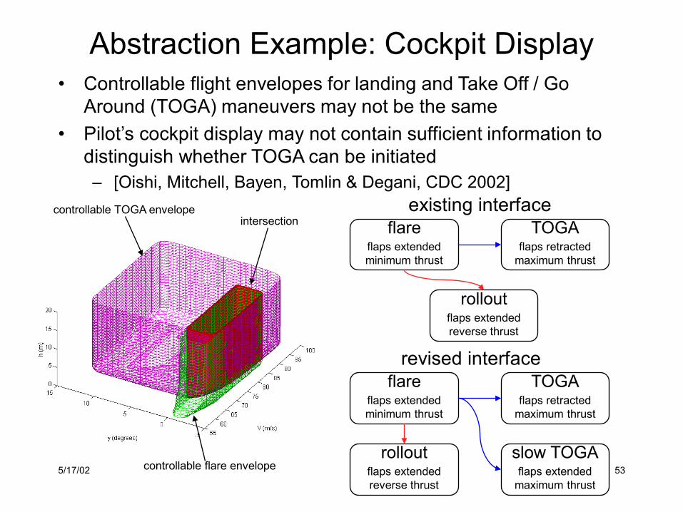
Abstraction Example: Cockpit Display• Controllable flight envelopes for landing and Take Off / Go
Around (TOGA) maneuvers may not be the same• Pilot’s cockpit display may not contain sufficient information to
distinguish whether TOGA can be initiated– [Oishi, Mitchell, Bayen, Tomlin & Degani, CDC 2002]
flareflaps extendedminimum thrust
rolloutflaps extendedreverse thrust
slow TOGAflaps extended
maximum thrust
TOGAflaps retracted
maximum thrust
flareflaps extendedminimum thrust
rolloutflaps extendedreverse thrust
TOGAflaps retracted
maximum thrust
revised interface
existing interface
controllable flare envelope
controllable TOGA envelopeintersection
5/17/02 54
Summary• Hybrid systems can model systems with complex interactions
between discrete and continuous components• Level set methods can accurately compute reachable sets for
nonlinear continuous and hybrid systems– Continuous and discrete inputs may affect system dynamics– Differential game formulation models unknown parameters robustly– Projective overapproximation to improve algorithm’s scalability
• These reachable sets can be applied to– Verify safe behavior– Synthesize safe control policies– Create discrete abstractions
• Reachability problems motivate innovation in level set methods– Particle level set method used for fluid simulation and animation
5/17/02 55
Future Directions• Comparing reachable sets computed by different algorithms
– Create interval or sector bounded linear approximation for landing example and compute control invariant subset of envelope (by LMIs & SDPs) or backwards reachable set (by ellipsoidal methods)
• Fully local level set implementation (time and space)• Toolkit for computing reachable sets• Control synthesis and planning
– Filtering controls for safety: soft walls for aircraft• Projective overapproximation
– Characterizing appropriate problems and choices of projections• Probabilistic models
5/17/02 56
Acknowledgements• Kaaren• Current & Former Supervisors
– Professors Claire Tomlin, Ronald Fedkiw & Mark Greenstreet• Committee
– Professors Stephen Boyd, David Dill & Antony Jameson• Hybrid Systems Lab
– Alexandre Bayen, Ronojoy Ghosh, Inseok Hwang, Gokhan Inalhan, Jung Soon Jang, Meeko Oishi, Dusan Stipanovic, Rodney Teo, Sherann Ellsworth
• Physically Based Modeling Group– Douglas Enright, Robert Bridson, Frederic Gibou, Eran
Guendelman, Neil Molino, Igor Neverov, Duc Nguyen, Joseph Teran
• Scientific Computing & Computational Mathematics Program• Family & Friends