Embed Size (px)
Citation preview

The Pennsylvania State University
The Graduate School
Department of Meteorology
APPLICATION OF IMAGE-PROCESSING TECHNIQUES FOR
DETERMINING CONVECTIVE BOUNDARY-LAYER DEPTH
FROM AEROSOL-LIDAR MEASUREMENTS
A Dissertation in
Meteorology
by
David O. Miller
© 2013 David O. Miller
Submitted in Partial Fulfillmentof the Requirements
for the Degree of
Doctor of Philosophy
December 2013

The dissertation of David O. Miller was read and approved∗ by the following:
Timothy J. KaneProfessor of Electrical EngineeringAdjunct Professor of MeteorologyDissertation AdviserChair of Committee
George Y. YoungProfessor of Meteorology
Sue Ellen HauptAdjunct Professor of Meteorology
Jack W. LangelaanAssociate Professor of Aerospace Engineering
William H. BruneDistinguished Professor of MeteorologyHead of the Department of Meteorology
∗Signatures on file in the Graduate School.

iii
Abstract
The convective boundary layer (CBL) plays a fundamental role in the exchangeof momentum, moisture, and sensible heat between the surface and the troposphere. Forthis reason, knowledge of the CBL is important to a wide range of disciplines includingmeteorology, air-quality, hydrology, wind energy, and aviation. Aerosol backscatter lidaris a valuable tool in the study of the CBL specifically in the determination of the CBLdepth. However, the common CBL-depth estimation methods, applied on a per-profilebasis, can be inadequate in identifying the transition zone at the top of the CBL due tomeasurement noise or lack of aerosol contrast between the CBL and the free-troposphere(i.e., the transition zone). Several image processing techniques are capable of identi-fying gradients and features in medical imagery and computer vision applications andby including temporal in addition to spatial information, it is found that these imageprocessing techniques can also be used to identify the transition zone in lidar data. Aprocess of matching the filter iterations to each estimator is developed and the resultsare merged improving the robustness of the estimates.

iv
Table of Contents
List of Tables . . . . . . . . . . . . . . . . . . . . . . . . . . . . . . . . . . . . . . vii
List of Figures . . . . . . . . . . . . . . . . . . . . . . . . . . . . . . . . . . . . . viii
Acknowledgments . . . . . . . . . . . . . . . . . . . . . . . . . . . . . . . . . . . xiii
Chapter 1. Introduction . . . . . . . . . . . . . . . . . . . . . . . . . . . . . . . . 11.1 The Convective Boundary Layer . . . . . . . . . . . . . . . . . . . . 11.2 CBL Depth Estimation . . . . . . . . . . . . . . . . . . . . . . . . . . 41.3 Motivation . . . . . . . . . . . . . . . . . . . . . . . . . . . . . . . . . 61.4 Research Goals . . . . . . . . . . . . . . . . . . . . . . . . . . . . . . 7
Chapter 2. Instrumentation . . . . . . . . . . . . . . . . . . . . . . . . . . . . . . 92.1 Measuring the CBL . . . . . . . . . . . . . . . . . . . . . . . . . . . . 92.2 Lidar Measurements of the CBL . . . . . . . . . . . . . . . . . . . . 102.3 The Holographic Airborne Rotating Lidar Instrument Experiment
(HARLIE) . . . . . . . . . . . . . . . . . . . . . . . . . . . . . . . . . 11
Chapter 3. Data Collection and Environment . . . . . . . . . . . . . . . . . . . . 143.1 Measurement Location . . . . . . . . . . . . . . . . . . . . . . . . . . 143.2 Radiosonde Data . . . . . . . . . . . . . . . . . . . . . . . . . . . . . 143.3 Lidar Data . . . . . . . . . . . . . . . . . . . . . . . . . . . . . . . . 143.4 Development Data Periods . . . . . . . . . . . . . . . . . . . . . . . . 15
3.4.1 Well-Defined CBL . . . . . . . . . . . . . . . . . . . . . . . . 163.4.2 Ill-defined CBL . . . . . . . . . . . . . . . . . . . . . . . . . . 173.4.3 Layers . . . . . . . . . . . . . . . . . . . . . . . . . . . . . . . 183.4.4 Clouds . . . . . . . . . . . . . . . . . . . . . . . . . . . . . . . 193.4.5 Data Gaps . . . . . . . . . . . . . . . . . . . . . . . . . . . . . 20
3.5 Synthetic Data . . . . . . . . . . . . . . . . . . . . . . . . . . . . . . 213.5.1 Idealized Profile . . . . . . . . . . . . . . . . . . . . . . . . . . 21
Chapter 4. Data Conditioning . . . . . . . . . . . . . . . . . . . . . . . . . . . . 254.1 Instrument Corrections . . . . . . . . . . . . . . . . . . . . . . . . . . 25
4.1.1 Detector Correction . . . . . . . . . . . . . . . . . . . . . . . 254.1.2 Azimuth Correction . . . . . . . . . . . . . . . . . . . . . . . 254.1.3 Background Subtraction . . . . . . . . . . . . . . . . . . . . . 274.1.4 Range Correction . . . . . . . . . . . . . . . . . . . . . . . . . 274.1.5 Cloud Mask . . . . . . . . . . . . . . . . . . . . . . . . . . . . 284.1.6 Gap Detection . . . . . . . . . . . . . . . . . . . . . . . . . . 29
4.2 Filter Introduction . . . . . . . . . . . . . . . . . . . . . . . . . . . . 304.3 Filter Description . . . . . . . . . . . . . . . . . . . . . . . . . . . . . 30

v
4.3.1 Gaussian Filter . . . . . . . . . . . . . . . . . . . . . . . . . . 314.3.2 Median Filter . . . . . . . . . . . . . . . . . . . . . . . . . . . 314.3.3 Wiener Filter . . . . . . . . . . . . . . . . . . . . . . . . . . . 314.3.4 Anisotropic Scalar Diffusion . . . . . . . . . . . . . . . . . . . 324.3.5 Speckle Reducing Anisotropic Diffusion . . . . . . . . . . . . 33
4.4 Filter Evaluation . . . . . . . . . . . . . . . . . . . . . . . . . . . . . 344.4.1 Idealized Profile Optimization . . . . . . . . . . . . . . . . . . 344.4.2 Contrast-to-Noise Ratio . . . . . . . . . . . . . . . . . . . . . 354.4.3 Filter Evaluation Method . . . . . . . . . . . . . . . . . . . . 35
4.5 Image Enhancement . . . . . . . . . . . . . . . . . . . . . . . . . . . 364.5.1 Contrast Stretching . . . . . . . . . . . . . . . . . . . . . . . 374.5.2 Histogram Normalization . . . . . . . . . . . . . . . . . . . . 374.5.3 Histogram Equalization . . . . . . . . . . . . . . . . . . . . . 38
Chapter 5. CBL Depth Estimation Methods . . . . . . . . . . . . . . . . . . . . 405.1 Radiosonde Estimation of CBL Depth . . . . . . . . . . . . . . . . . 405.2 One-Dimensional Methods . . . . . . . . . . . . . . . . . . . . . . . . 40
5.2.1 Derivatives . . . . . . . . . . . . . . . . . . . . . . . . . . . . 415.2.2 Edge Detection . . . . . . . . . . . . . . . . . . . . . . . . . . 415.2.3 Haar Wavelet . . . . . . . . . . . . . . . . . . . . . . . . . . . 415.2.4 Idealized Profile . . . . . . . . . . . . . . . . . . . . . . . . . . 42
5.3 Two-Dimensional Methods . . . . . . . . . . . . . . . . . . . . . . . . 425.3.1 Morphological Operators . . . . . . . . . . . . . . . . . . . . . 435.3.2 Edge Detection . . . . . . . . . . . . . . . . . . . . . . . . . . 435.3.3 Active Contours . . . . . . . . . . . . . . . . . . . . . . . . . 445.3.4 k-Means Clustering . . . . . . . . . . . . . . . . . . . . . . . . 45
5.4 Location of zi within the Transition Zone . . . . . . . . . . . . . . . 455.5 Human Estimation of CBL Depth . . . . . . . . . . . . . . . . . . . . 45
Chapter 6. Results . . . . . . . . . . . . . . . . . . . . . . . . . . . . . . . . . . . 476.1 Filter Results . . . . . . . . . . . . . . . . . . . . . . . . . . . . . . . 47
6.1.1 Well-Defined CBL . . . . . . . . . . . . . . . . . . . . . . . . 476.1.2 Ill-Defined CBL . . . . . . . . . . . . . . . . . . . . . . . . . . 486.1.3 Layers . . . . . . . . . . . . . . . . . . . . . . . . . . . . . . . 496.1.4 Clouds . . . . . . . . . . . . . . . . . . . . . . . . . . . . . . . 506.1.5 Data Gaps . . . . . . . . . . . . . . . . . . . . . . . . . . . . . 516.1.6 Synthetic Data . . . . . . . . . . . . . . . . . . . . . . . . . . 526.1.7 Filter Discussion and Selection . . . . . . . . . . . . . . . . . 53
6.2 CBL Estimator Discussion . . . . . . . . . . . . . . . . . . . . . . . . 556.3 Merging Estimates . . . . . . . . . . . . . . . . . . . . . . . . . . . . 596.4 Filter-Estimator Matching . . . . . . . . . . . . . . . . . . . . . . . . 606.5 CBL Estimator Results . . . . . . . . . . . . . . . . . . . . . . . . . 61
6.5.1 Well Defined CBL . . . . . . . . . . . . . . . . . . . . . . . . 616.5.2 Ill-Defined CBL . . . . . . . . . . . . . . . . . . . . . . . . . . 626.5.3 Layers . . . . . . . . . . . . . . . . . . . . . . . . . . . . . . . 63

vi
6.5.4 Clouds . . . . . . . . . . . . . . . . . . . . . . . . . . . . . . . 646.5.5 Data Gaps . . . . . . . . . . . . . . . . . . . . . . . . . . . . . 656.5.6 Synthetic Data . . . . . . . . . . . . . . . . . . . . . . . . . . 666.5.7 Discussion of CBL Estimator Results . . . . . . . . . . . . . . 68
6.6 Comparison with Human Estimates of CBL Depth . . . . . . . . . . 696.6.1 Discussion of Human and Estimator Comparisons . . . . . . . 77
Chapter 7. Conclusions . . . . . . . . . . . . . . . . . . . . . . . . . . . . . . . . 807.1 Assessment of Goals . . . . . . . . . . . . . . . . . . . . . . . . . . . 807.2 Future Work . . . . . . . . . . . . . . . . . . . . . . . . . . . . . . . 81
Appendix A.CBL Top Estimation GUI . . . . . . . . . . . . . . . . . . . . . . . . 83
Bibliography . . . . . . . . . . . . . . . . . . . . . . . . . . . . . . . . . . . . . . 87

vii
List of Tables
1.1 Methods for determining the CBL depth (Beyrich, 1997) . . . . . . . . . 5
4.1 The parameters and the range for each of the five filters evaluated in thisstudy. . . . . . . . . . . . . . . . . . . . . . . . . . . . . . . . . . . . . . 33
6.1 The period number, campaign and date, root mean square difference be-tween human and merged estimates (RMSD), mean standard deviation ofestimates for the human (σhuman) estimates, mean range of estimates forthe human (Rhuman) and merged (Rmerged) estimates for the 17 human-assessed periods. . . . . . . . . . . . . . . . . . . . . . . . . . . . . . . . 79

viii
List of Figures
1.1 Fair-weather cumulus clouds sitting on top of the convective boundarylayer (CBL). Significant transport of moisture and aerosols occurs viathe CBL. (Namek, 2005) . . . . . . . . . . . . . . . . . . . . . . . . . . . 2
1.2 Aerosol backscatter lidar profile. The decrease in normalized backscatterintensity at ∼ 1.8km is a result of the decrease in aerosols from the CBLto the free atmosphere. . . . . . . . . . . . . . . . . . . . . . . . . . . . . 3
1.3 Diurnal evolution of the atmospheric boundary layer (ABL) which in-cludes the CBL (NikNaks, 2012). . . . . . . . . . . . . . . . . . . . . . . 4
2.1 Left: Holographic Airborne Rotating Lidar Instrument Experiment (HAR-LIE) in its ground-based configuration. Right: Holographic Optical El-ement (HOE) used to collect and focus the backscattered photons. TheHOE is rotated during measurements producing a conical scan of theatmosphere. . . . . . . . . . . . . . . . . . . . . . . . . . . . . . . . . . . 12
2.2 A single scan of the HARLIE instrument showing the conical pattern(lower left) and an azimuth vs. altitude representation (upper right). . . 13
3.1 A normalized aerosol backscatter intensity profile vs. altitude. . . . . . . 153.2 A backscatter intensity image. . . . . . . . . . . . . . . . . . . . . . . . . 163.3 Left: Aerosol backscatter from 11 June 2002 during the IHOP field cam-
paign. Right: Potential temperature profile (θ) derived from the ra-diosonde launch at 1739 UTC. The CBL is well mixed therefore θ isnearly constant within the CBL and increases above zi. . . . . . . . . . 17
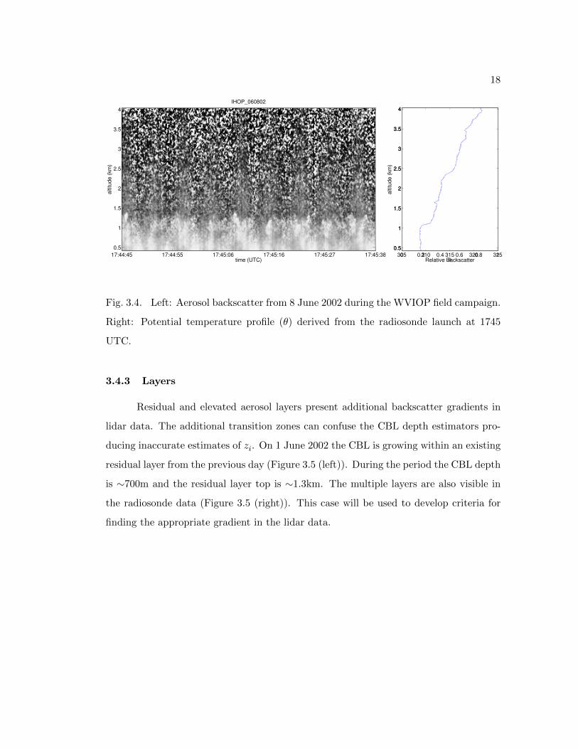
3.4 Left: Aerosol backscatter from 8 June 2002 during the WVIOP fieldcampaign. Right: Potential temperature profile (θ) derived from theradiosonde launch at 1745 UTC. . . . . . . . . . . . . . . . . . . . . . . 18
3.5 Left: Aerosol backscatter from 1 June 2002 during the WVIOP fieldcampaign. The periodicity is due to the HARLIE instrument repeat-edly measuring the same atmospheric features as it is scanned. Right:Potential temperature profile (θ) derived from the radiosonde launch at1752 UTC. Multiple layers are visible in this profile making it an idealcandidate for testing the radiosonde zi estimate algorithms. . . . . . . . 19
3.6 Left: Aerosol backscatter from 6 October 2000 during the WVIOP fieldcampaign with a cloud layer visible at ∼ 3.2km. Right: Potential tem-perature profile (θ) derived from the radiosonde launch at 1732 UTC. . 20
3.7 Left: Aerosol backscatter from 2 June 2002 during the IHOP field cam-paign. Note the dropouts and vertical shifts in the data. Right: Potentialtemperature profile (θ) derived from the radiosonde launch at 1727 UTC. 21
3.8 Left: An ideal aerosol-backscatter intensity profile. Right: An idealbackscatter intensity profile with a correction for the strong near-rangebackscatter. . . . . . . . . . . . . . . . . . . . . . . . . . . . . . . . . . . 23

ix
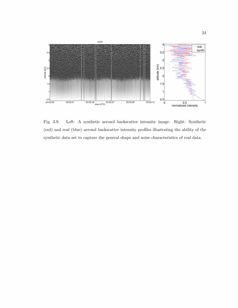
3.9 Left: A synthetic aerosol backscatter intensity image. Right: Synthetic(red) and real (blue) aerosol backscatter intensity profiles illustrating theability of the synthetic data set to capture the general shape and noisecharacteristics of real data. . . . . . . . . . . . . . . . . . . . . . . . . . 24
4.1 Normalized azimuth-dependent intensity variation for the WVIOP cam-paign. . . . . . . . . . . . . . . . . . . . . . . . . . . . . . . . . . . . . . 26
4.2 Normalized azimuth-dependent intensity variation for the IHOP campaign. 274.3 A quicklook image showing the effect of the azimuth angle correction. . 284.4 The idealized-backscatter profile (red line) fit to an aerosol-backscatter
profile (black line). . . . . . . . . . . . . . . . . . . . . . . . . . . . . . . 344.5 The transition zone thickness (TZT) vs. contrast-to-noise ratio (CNR)
for five filters from 11 June 2002 during the IHOP field campaign (Well-defined CBL). The filters are as follows: Gauss=2D Gaussian; Median=2DMedian; Wiener=2D Wiener; Sdiff=2D anisotropic scalar diffusion; SRAD=SpeckleReducing Anisotropic Diffusion. Application of a filter will, ideally, de-crease TZT and increase CNR. . . . . . . . . . . . . . . . . . . . . . . . 36
4.6 Left: Aerosol-backscatter image showing the results of contrast stretch-ing. Right: Histogram of image intensities with a range from 0 to 1. . . 37
4.7 Left: Aerosol-backscatter image showing the results of histogram nor-malization. Right: Histogram of image intensities after histogram nor-malization. . . . . . . . . . . . . . . . . . . . . . . . . . . . . . . . . . . 38
4.8 Left: Aerosol-backscatter image showing the results of histogram normal-ization. Right: Histogram of image intensities after histogram equalization. 39
6.1 The transition zone thickness (TZT) vs. contrast-to-noise ratio (CNR)for five filters from 11 June 2002 during the IHOP field campaign (Well-defined CBL). The filters are as follows: Gauss=2D Gaussian; Median=2DMedian; Wiener=2D Wiener; Sdiff=2D anisotropic scalar diffusion; SRAD=SpeckleReducing Anisotropic Diffusion. . . . . . . . . . . . . . . . . . . . . . . . 48
6.2 The transition zone thickness (TZT) vs. contrast-to-noise ratio (CNR)for five filters from 11 June 2002 during the IHOP field campaign (Ill-defined CBL). The filters are as follows: Gauss=2D Gaussian; Median=2DMedian; Wiener=2D Wiener; Sdiff=2D anisotropic scalar diffusion; SRAD=SpeckleReducing Anisotropic Diffusion. . . . . . . . . . . . . . . . . . . . . . . . 49
6.3 The entrainment zone thickness (EZT) vs. contrast-to-noise ratio (CNR)for five filters from 01 June 2002 during the IHOP field campaign (Lay-ers). The filters are as follows: Gauss=2D Gaussian; Median=2D Me-dian; Wiener=2D Wiener; PM=2D Perona Malik scalar diffusion; Td-iff=2D tensor diffusion. . . . . . . . . . . . . . . . . . . . . . . . . . . . 50
6.4 The transition zone thickness (TZT) vs. contrast-to-noise ratio (CNR)for five filters from 11 June 2002 during the IHOP field campaign (Clouds).The filters are as follows: Gauss=2D Gaussian; Median=2D Median;Wiener=2D Wiener; Sdiff=2D anisotropic scalar diffusion; SRAD=SpeckleReducing Anisotropic Diffusion. . . . . . . . . . . . . . . . . . . . . . . . 51
x
6.5 The transition zone thickness (TZT) vs. contrast-to-noise ratio (CNR)for five filters from 11 June 2002 during the IHOP field campaign (Gaps).The filters are as follows: Gauss=2D Gaussian; Median=2D Median;Wiener=2D Wiener; Sdiff=2D anisotropic scalar diffusion; SRAD=SpeckleReducing Anisotropic Diffusion. . . . . . . . . . . . . . . . . . . . . . . . 52
6.6 The transition zone thickness (TZT) vs. contrast-to-noise ratio (CNR)for five filters from 11 June 2002 during the IHOP field campaign. The fil-ters are as follows: Gauss=2D Gaussian; Median=2D Median; Wiener=2DWiener; Sdiff=2D anisotropic scalar diffusion; SRAD=Speckle ReducingAnisotropic Diffusion. . . . . . . . . . . . . . . . . . . . . . . . . . . . . 53
6.7 Segments of aerosol-backscatter intensity images showing the effects ofthe Wiener, SDIFF, and SRAD filters . . . . . . . . . . . . . . . . . . . 54
6.8 Aerosol-backscatter image showing the performance of the first-derivativeCBL depth estimator . . . . . . . . . . . . . . . . . . . . . . . . . . . . . 56
6.9 Aerosol-backscatter image showing the performance of the wavelet CBLdepth estimator . . . . . . . . . . . . . . . . . . . . . . . . . . . . . . . . 57
6.10 Aerosol-backscatter image showing the performance of the idealized-profileCBL depth estimator . . . . . . . . . . . . . . . . . . . . . . . . . . . . . 58
6.11 Aerosol-backscatter image showing the performance of the active-contourCBL depth estimator . . . . . . . . . . . . . . . . . . . . . . . . . . . . . 59
6.12 The top plot shows the mean range of CBL depth estimator values foreach of the development periods. The bottom plot shows the number ofiterations of the SDIFF filter matched to each CBL depth estimator. . . 61
6.13 Left: Aerosol-backscatter image for 11 June 2002 (well-defined CBL)with the merged CBL depth estimates (red line) and the range of theCBL depth estimators (orange line). Right: Potential-temperature pro-file (blue line) and aerosol-backscatter profile (red line), from the centerof the period, and the merged CBL depth estimator result (red dashedline). . . . . . . . . . . . . . . . . . . . . . . . . . . . . . . . . . . . . . . 62
6.14 Left: Aerosol-backscatter image for 8 June 2002 (ill-defined CBL) withthe merged CBL depth estimates (red line) and the range of the CBLdepth estimators (orange line). Right: Potential-temperature profile(blue line) and aerosol-backscatter profile (red line), from the center ofthe period, and the merged CBL depth estimator result (red dashed line). 63
6.15 Left: Aerosol-backscatter image for 1 June 2002 (Layers) with the mergedCBL depth estimates (red line) and the range of the CBL depth estima-tors (orange line). Right: Potential-temperature profile (blue line) andaerosol-backscatter profile (red line), from the center of the period, andthe merged CBL depth estimator result (red dashed line). . . . . . . . . 64
6.16 Left: Aerosol-backscatter image for 6 October 2000 (Clouds) with themerged CBL depth estimates (red line) and the range of the CBL depthestimators (orange line). Right: Potential-temperature profile (blue line)and aerosol-backscatter profile (red line), from the center of the period,and the merged CBL depth estimator result (red dashed line). . . . . . . 65

xi
6.17 Left: Aerosol-backscatter image for 2 June 2002 (Data Gaps) with themerged CBL depth estimates (red line) and the range of the CBL depthestimators (orange line). Right: Potential-temperature profile (blue line)and aerosol-backscatter profile (red line), from the center of the period,and the merged CBL depth estimator result (red dashed line). . . . . . . 66
6.18 Left: Aerosol-backscatter image for the synthetic data set with the mergedCBL depth estimates (red line) and the range of the CBL depth estima-tors (orange line). Right: Aerosol-backscatter profile (red line), from thecenter of the period, and the merged CBL depth estimator result (reddashed line). . . . . . . . . . . . . . . . . . . . . . . . . . . . . . . . . . 67
6.19 Aerosol-backscatter image for the synthetic data set with the mergedCBL depth estimates (red line) and the actual zi values (green line). . . 68
6.20 Aerosol-backscatter image showing the results of the human (blue line)and merged (red line) CBL depth estimates for 4 October 2000. . . . . . 69
6.21 Aerosol-backscatter image showing the results of the human (blue line)and merged (red line) CBL depth estimates for 4 October 2000. Thelight blue lines indicate the range of human estimates for the period. . . 70
6.22 Aerosol-backscatter image showing the results of the human (blue line)and merged (red line) CBL depth estimates for 20 September 2000. . . . 71
6.23 Aerosol-backscatter image showing the results of the human (blue line)and merged (red line) CBL depth estimates for 20 September 2000. Thelight blue lines indicate the range of human estimates for the period. . . 72
6.24 Aerosol-backscatter image showing the results of the human (blue line)and merged (red line) CBL depth estimates for 21 September 2000. Theorange lines indicate the range of the CBL depth estimators. . . . . . . 73
6.25 Aerosol-backscatter image showing the results of the human (blue line)and merged (red line) CBL depth estimates for 21 September 2000. Thelight blue lines indicate the range of human estimates for the period . . 74
6.26 Aerosol-backscatter image showing the results of the human (blue line)and merged (red line) CBL depth estimates for 6 October 2000. Theorange lines indicate the range of the CBL depth estimators. . . . . . . 75
6.27 Aerosol-backscatter image showing the results of the human (blue line)and merged (red line) CBL depth estimates for 6 October 2000. Thelight-blue lines indicate the range of the human CBL depth estimates. . 76
6.28 Potential-temperature profile (blue line) and aerosol-backscatter profile(red line), from the center of the period. The merged CBL depth esti-mator result (red dashed line) and the average of the human estimates(dashed blue line) are also shown. . . . . . . . . . . . . . . . . . . . . . . 77
6.29 The top plot shows the mean range of CBL depth estimator values foreach of the periods. The bottom plot shows the number of iterations ofthe SDIFF filter matched to each CBL depth estimator. . . . . . . . . . 78

xii
A.1 Radiosonde potential temperature (θ) profile. Potential temperature istypically constant within the convective boundary layer (CBL) and in-creases above the CBL. The horizontal line indicates the estimated topof the CBL (zi). . . . . . . . . . . . . . . . . . . . . . . . . . . . . . . . . 86

xiii
Acknowledgments
I want to start by thanking Geary Schwemmer and all of my colleagues at NASAGoddard Space Flight Center for getting my meteorological career off to a great start andproviding me with years of engaging research. My affinity for measuring the atmospherewas a result of my time at NASA. Also, this research and my career at Penn State waskickstarted by NASA grant ShADOE: Engineering and Science Applications for which Iam grateful.
Thank you to my advisor, Dr. Tim Kane, for enabling me to establish my careerat Penn State by encouraging me to resume my studies, supporting me at the start, andfor guiding me over the many years it has taken me to get to this point. Thank youto Dr. George Young for taking me under your wing and guiding me to the end withgreat efficiency. And thanks to Drs. Sue Haupt and Jack Langelaan for your guidanceand suggestions. I am also appreciative of Dr. William Brune for giving me the time tocomplete this research.
Finally, a special thank you to my wife, Sonya, for riding this train with me.Without your patience, support, and love I would have never achieved this goal. Tomy daughters, Audra and Margot, thank you for making me proud and keeping megrounded. And thank you to my parents, Ralph and Sheila, for supporting my collegecareer and their unending encouragement.

1
Chapter 1
Introduction
1.1 The Convective Boundary Layer
A definition of the atmospheric boundary layer (ABL) is given by Garratt (1994)
as the “layer of air directly above the Earth’s surface in which the effects of the surface
(e.g., friction, heating, and cooling) are felt directly on times scales less than a day, and in
which significant fluxes of momentum, heat or matter are carried by turbulent motions on
a scale of the order of the depth of the boundary layer or less.” In particular, knowledge
of the depth of the convective boundary layer (CBL) provides a vertical dimension over
which the transport processes occur (Lammert and Bosenberg, 2006) and is valuable
to a wide range of disciplines including, but not limited to, atmospheric transport and
diffusion, mesoscale modeling, aviation, wind energy, and oceanography. A common
feature of the CBL is fair-weather cumulus clouds that form as rising parcels of air cool
resulting in condensation (Figure 1.1).
Arya (1988) states, “A boundary layer is defined as the layer of fluid in the im-
mediate vicinity of a material surface in which significant exchange of momentum, heat,
or mass takes place between the surface and the fluid.” With respect to the atmosphere,
the boundary layer can be defined as the lower portion of the troposphere that is di-
rectly influenced by the turbulent exchange of momentum, moisture, and sensible heat
between the surface and atmosphere with a timescale of roughly a few hours (Stull,
1988). Anthropogenic emissions released at the surface are mixed throughout the CBL
via turbulent motions.
Several names are often used when referring to the boundary layer. The terms
convective boundary layer (CBL) and mixing layer (ML) are equivalent and are often
used in atmospheric transport studies. At night, the boundary layer becomes statically
stable with only weak and intermittent turbulence and is called the stable boundary

2
Fig. 1.1. Fair-weather cumulus clouds sitting on top of the convective boundary layer(CBL). Significant transport of moisture and aerosols occurs via the CBL. (Namek, 2005)
layer (SBL) or nocturnal boundary layer (NBL). The terms planetary boundary layer
(PBL) and atmospheric boundary layer (ABL) are more general and can include both
the CBL and SBL. This research will focus on the established CBL.
There is a transition from aerosol-laden air to relatively clean free-atmosphere air
(Figure 1.2) at the top of the CBL and within this transition zone free-atmosphere air
entrains into the CBL (Trumner et al., 2011) causing the increase in CBL depth. The
diurnal evolution of the atmospheric boundary layer, which includes the CBL, is shown
in Figure 1.3. The transition zone is also the entrainment zone (EZ) but care should be
taken in regards to the various available definitions of EZ. Deardorff et al. (1980) defined,
what has become, one of the most common definitions of the EZ where they defined the
top of the EZ as the height that is occupied by CBL thermals around 5% of the time
and the bottom as the height occupied by CBL thermals 90-95% of the time. This is a
statistical definition of the EZ and doesn’t necessarily correspond to the mean transition-
zone thickness (Cohn and Angevine, 2000). The combination of higher-resolution CBL

3
measurements and models has increased the interest in defining the actual nature of the
EZ (Davis et al., 1997; Hageli et al., 2000; Grabon et al., 2010).
0.1 0.2 0.3 0.4 0.5 0.60
0.5
1
1.5
2
2.5
3
3.5
4
4.5
normalized intensity
altitud
e (
km
)
Fig. 1.2. Aerosol backscatter lidar profile. The decrease in normalized backscatterintensity at ∼ 1.8km is a result of the decrease in aerosols from the CBL to the freeatmosphere.
There is no universally accepted definition of CBL depth (Seibert et al., 1997).
Various processes (e.g., advection, radiation, and turbulence) define the structure of the
CBL and affect vertical profiles of CBL parameters in unique ways (Beyrich, 1997). Also,
definitions of CBL depth are products of the instruments used to measure the defining
parameters of the CBL. Beyrich (1997) lists ten methods of the determining CBL depth
from measurements (Table 1.1). Lidar backscatter is proportional to aerosol concen-
tration so the definition “Height at which moisture or aerosol concentration suddenly
decreases” will be used in this study. It should be noted that there are known discrep-
ancies between lidar estimated and radiosonde temperature derived zi heights (Coulter,
1979), because the rising air parcels, due to their momentum, do not stop immediately
when they become neutrally buoyant.

4
Fig. 1.3. Diurnal evolution of the atmospheric boundary layer (ABL) which includesthe CBL (NikNaks, 2012).
1.2 CBL Depth Estimation
The CBL depth can be measured in situ via balloon-borne or tethered sondes
and aircraft or remotely via sodar, radar, lidar, and wind-profilers (Clifford et al., 1994;
Seibert et al., 2000). The well-mixed nature of the CBL results in relatively uniform
aerosol concentrations within the CBL with a decrease in concentration at the CBL top,
zi. This transition-zone gradient is used to estimate zi in aerosol lidar data (Melfi et al.,
1985).
Many methods have been developed to estimate zi from lidar data with rela-
tively good success (Kovalev and Eichinger, 2004). However, any factor that reduces the
aerosol contrast between the CBL and free troposphere will reduce the effectiveness of
the technique. For example, the CBL growing through the previous day’s residual layer
or the advection of aerosols from outside the measurement region can result in decreased
transition-zone contrast. To reduce the effects of noise the backscatter profiles are often
temporally and spatially averaged before analysis. The averaging process necessarily re-
duces the resolution of the data and may not entirely eliminate the noise. Discontinuities

5
Table 1.1. Methods for determining the CBL depth (Beyrich, 1997)
CBL-depth based on profiles of mean vari-ables (wind, temperature, humidity, con-centrations)
CBL-depth based on profiles of turbulentvariables (fluxes, variances, TKE, struc-ture parameters)
• Height of a zone with significant windshear
• Height where the turbulent heat fluxchanges sign
• Base of an elevated inversion • Height at which the turbulent heat fluxhas a negative maximum
• Height at which a rising air parcel be-comes neutrally buoyant
• Height at which TKE dissipation rateor vertical velocity variance significantlydecreases
• Height at which moisture or aerosol con-centration suddenly decreases
• Height of an elevated maximum ofacoustic/electromagnetic refractive indexparameters
• Height at which single plume verticalvelocity vanishes
• Similarity methods based on profilemeasurements within the mixing layer
in the zi estimates between profiles can arise depending on the response of the technique
to the noise.
A commonly employed method to reduce the noise in lidar data is to temporally
average the backscatter profiles for a specific period of time. This method does reduce
the amount of noise at the expense of temporal resolution in the data and can also
blur the transition-zone gradient possibly making detection more difficult. The length of
the time-average varies and depends on the instrument details and intended use of the
data. Martucci et al. (2010) produced zi estimates for use in numerical models with a
30 minute temporal and 12m altitude resolution using data from a relatively low power
lidar system. Conversely, Grabon et al. (2010) used data from a high-power aircraft
lidar to develop a data set of zi estimates with 15m temporal and altitude resolution
for studying entrainment-zone thickness. Another method is to filter the data in one or
two spatial dimensions. This maintains the temporal resolution of the data with some
degradation in spatial resolution. The amount of spatial resolution degradation depends
on the sophistication of the filter being employed.

6
A drawback to most of the current CBL estimating methods is in how they are
applied: on a per-profile basis. This application requires the profile to have a well-defined
transition-zone gradient to be successful. However, a researcher visually examining a
time-altitude intensity image of aerosol backscatter can often discern zi, even for data
with high levels of noise and missing data. This is the primary motivation of this research:
that mathematically mimicking the visual capabilities of a human in analyzing lidar
data for CBL features can be beneficial to the science. Much like visual analysis, image
processing methods incorporate spatial and temporal information to improve the retrieval
of the transition zone.
1.3 Motivation
Estimates of zi from lidar data, aerosol and otherwise, is a decades-old science and
there are several widely accepted and successfully employed methods in use today. But
all of these methods are one-dimensional and require good signal CNR to be successful.
Judicious averaging of the data or using lidar systems with inherent high CNR is required
to produce acceptable estimates of zi using 1-D estimators. The resolution of zi estimates
currently satisfies the needs of the modeling community, however, this reality is slowly
changing. Atmospheric models are rapidly increasing in resolution and eventually current
estimates will not suffice. Also, the number of lidars in use around the world is increasing.
Many of these new lidars are low-power (i.e., lower CNR) systems such as ceilometers
and new methods, with lower averaging requirements, must be developed to estimate zi.
The image processing methods used in this study are effective at finding features
in images. They have been utilized in the medical and computer-vision communities
for, in some cases, decades (Deklerck et al., 1993; Staib and Duncan, 1996). Magnetic
Resonance Imaging (MRI), for example, is used to image tissues inside the human body
for patient diagnostics (Hendee and Morgan, 1984). The images produced from the MRI
show tissues in shades of gray with varying amounts of contrast, similar to the aerosol
backscatter images used in this study. Image segmentation assists medical professionals
by identifying structures in the MRI images (Balafar et al., 2010) so the application to
aerosol lidar data is a natural step. This application, however, has seen little activity in

7
the atmospheric-science community. Haeffelin et al. (2012) used a Sobel edge detector
along with a selection of 1-D zi estimation methods and Parikh and Parikh (2002) used
both the Canny edge detector and a customized active contour to find CBL top in lidar
data. The relative lack of published work in this topic, coupled with the growing need for
high-resolution zi estimates, means additional research in this application is warranted.
1.4 Research Goals
The proposed research fulfills the following tasks:
• Investigate the use of advanced filtering methods to reduce the amount of temporal
and spatial averaging necessary prior to application of zi estimators
• Successfully retrieve zi using a selection of image processing methods
• Produce a robust estimate of zi that, at a minimum, is comparable to human esti-
mation of zi in aerosol lidar data
All CBL estimation methods benefit from increased contrast-to-noise ratio (CNR) and,
to accomplish this goal, a fair amount of time was devoted to conditioning the data prior
to application of the estimators. A selection of filters was investigated with the goal
of reducing noise while preserving features. A set of community-accepted zi estimation
methods is applied to the data along with several image processing methods. The im-
age processing methods were modified and tuned to successfully estimate zi from noisy
lidar data. In addition, the zi estimators are matched with a specific filter for optimal
performance and then the estimates were merged to produce a robust estimate of zi. A
GUI was developed to allow individuals to estimate CBL depth via visual analysis of the
data. Comparing the automated estimates to the human truth estimates, in addition
to coincident radiosonde measurements, reveals the accuracy of the automated meth-
ods. As expected, the research did not return a single estimator that is useful for all
datasets. Rather, the strengths of each estimator are leveraged through filter matching
and merging.
Joffre et al. (2001) states that one of the primary sources of error in weather and
climate models stems from inadequate parametrization of the CBL. A potential benefit

8
of this research is the ability to use lower power lidar systems (i.e., smaller and cheaper)
for CBL studies. This application has been demonstrated, with limited success, with
ceilometer systems by Eresmaa et al. (2006). Using the proposed methods to estimate
CBL depth from ceilometer measurements may increase the resolution of CBL depth
and transition-zone thickness estimates.

9
Chapter 2
Instrumentation
2.1 Measuring the CBL
There are several instruments that can be used to measure the CBL, and Seibert
et al. (2000) provides an extensive comparison of these instruments. Measurements can
be split into two types: in-situ and remote sensing. In situ measurements include balloon-
based radiosonde, aircraft, and tower measurements. Radiosondes are commonly used to
estimate zi from temperature, humidity, and velocity profiles but are limited by coarse
vertical resolution and infrequent launches. In addition, they tend to drift downwind, so
the time when they reach zi may not be at the desired location. However, radiosonde
estimates of zi are still considered to be a community standard and will be used as one
benchmark in this study. Tethered balloons can measure the turbulent, thermodynamic,
and chemical characteristics at zi directly but have a limited altitude range so are not
well suited for CBL depth in excess of 0.5 − 1.0km. Aircraft measurements cover a
relatively large area but cannot be used to monitor the evolution of the CBL at fixed
locations.
In contrast, remote sensors can offer continuous profiles of atmospheric charac-
teristics. Sodars measure the fluctuations in the acoustic refractive index and are well
suited for SBL studies. The limited vertical range, however, makes them unsuitable for
CBL studies (Beyrich, 1997). Radar wind profilers operate in a similar fashion to sodars
except in the radio-frequency portion of the electromagnetic spectrum. These instru-
ments can also reveal profiles of temperature and moisture fluctuations. Moisture is not
as well-mixed as aerosols nor is it a conserved quantity in the CBL therefore zi estimates
from radar may be difficult.
There are several types of lidars but aerosol backscatter systems are typically
used for CBL studies and can be ground, aircraft, or satellite-based. Satellite-based

10
lidars usually have relatively low-resolution range bins because of the distances they
need to cover to reach the ground. Also, they orbit at a high velocity and, while they
provide global coverage, provide relatively few local measurements. So, for CBL studies,
ground and aircraft-based lidars are the most common.
2.2 Lidar Measurements of the CBL
Light detection and ranging (lidar) is a remote-sensing measurement technique
where a light pulse is emitted into the atmosphere and the returned energy is measured
and analyzed to deduce characteristics of the atmosphere (Weitkamp, 2005). There are
two primary components to a lidar system: a transmitter and receiver. The transmit-
ter is usually a laser that provides the light pulses that are delivered either directly or
through various optics to the atmosphere with the wavelength of the laser depending
on the application. Raman lidar, for example, uses laser wavelengths that excite spe-
cific molecules that emit a characteristic shifted wavelength that can then be measured.
Aerosol-backscatter lidars use a variety of wavelengths but typically operate at 355, 532,
or 1064nm. (Kovalev and Eichinger, 2004). A telescope (i.e., the receiver) collects the
backscattered photons and they are delivered to a highly-sensitive detector and digitizer
that counts the individual photons and bins them based on their arrival time. Lidar mea-
surements yield a relatively small amount of energy returned to the receiver so larger
telescopes can be advantageous. However, background light can become increasingly
problematic with larger telescope apertures because of the increased field of view. Also,
the use of a large telescope may not be possible (e.g., on an aircraft) or practical (e.g.,
telescope cost). Lidars provide range-resolved profiles of the property being measured.
The profiles are proportional to the concentration of aerosols with an aerosol-backscatter
lidar. Unless the system is self-calibrated or a secondary measurement of aerosol extinc-
tion is provided, the backscatter intensity profiles are relative.
Aerosols are usually well mixed in the CBL, and there is often a relatively sharp
decrease in aerosol concentration when transitioning from the CBL to the free atmosphere
(FA). Rising thermals impinging on the stable layer above the CBL tend to compress
this transition zone making its signature in lidar data relatively sharp and easy to detect

11
and descending air can mix down free-atmosphere air stretching and diffusing the tran-
sition zone making its detection via lidar more difficult. Measuring the location of this
transition zone is an indicator of the top of the CBL and measurements of the vertical
distribution of aerosols make lidar an excellent tool for estimating the top of the CBL.
2.3 The Holographic Airborne Rotating Lidar Instrument Experiment
(HARLIE)
The data used in this study were collected with the Holographic Airborne Rotating
Lidar Instrument Experiment (HARLIE) (Figure 2.1 (Left)). Schwemmer (1998) gives
a detailed description of HARLIE. In summary, HARLIE is an aerosol backscatter lidar
operating at 1064 nm with a 40 cm holographic optical element (HOE) that is used as
the primary collecting and focusing optic (Figure 2.1 (Right)). The HARLIE instrument
employs a novel measurement scan pattern for observing the distribution of atmospheric
aerosols (Schwemmer et al., 2001). The HOE has a 45-degree diffraction angle and
rotates during operation resulting in a conical scan of the atmosphere (Figure 2.2). Data
is collected at the 5 kHz laser pulse repetition rate and averaged every 500 shots resulting
in 10 Hz data. The range resolution of the lidar is 30m and, with an elevation angle of
45◦, yields a vertical resolution of roughly 21m.

12
Fig. 2.1. Left: Holographic Airborne Rotating Lidar Instrument Experiment (HARLIE)
in its ground-based configuration. Right: Holographic Optical Element (HOE) used to
collect and focus the backscattered photons. The HOE is rotated during measurements
producing a conical scan of the atmosphere.
Scanning lidar systems have been used to great advantage in numerous CBL
studies (Kunkel et al., 1977; Piironen and Eloranta, 1995). One benefit of using scanning
versus static, zenith pointing lidar data is the increased horizontal sampling resolution.
The dimensions of the thermals defining the CBL scale horizontally with the depth of
the CBL by a factor of ∼ 1.5zi. Assuming zi = 1000m the horizontal scale of the
thermals is λ ≈ 1500m. If the mean wind speed is u = 5ms it will take approximately
300s for a typical feature to pass over a location. The HARLIE instrument typically
scans at 30◦/s, and at 1km altitude, results in roughly 52m between profiles or about 30
profiles sampling a single thermal in 3s. When filtering to reduce data noise, the higher
horizontal sampling resolution provided by a scanning lidar results in less information
loss compared to static lidar measurements.

13
Fig. 2.2. A single scan of the HARLIE instrument showing the conical pattern (lowerleft) and an azimuth vs. altitude representation (upper right).

14
Chapter 3
Data Collection and Environment
3.1 Measurement Location
The data used in this study were collected during two field campaigns. The first
campaign was held at the Atmospheric Radiation Measurement (ARM) Program’s Cloud
and Radiation Testbed (CART) Southern Great Plains (SGP) site in Oklahoma. This
site was created to provide data for model development and satellite validation (Stokes
and Schwartz, 1994). The Water Vapor Intensive Observation Period (WVIOP) 2000
field campaign was held 18 Sep. - 8 Oct. 2000 at the ARM CART site in Oklahoma with
the goal of the measuring water vapor in the lower troposphere and thereby improving
the calculations of downwelling radiance at the surface (Revercomb et al., 2003). The
second campaign was the International H2O Project (IHOP) held from 13 May - 25 Jun.
2002 in the panhandle of Oklahoma. The purpose of IHOP was to characterize the four-
dimensional distribution of water vapor to better understand its impact on convection.
3.2 Radiosonde Data
Radiosonde data from both field campaigns used in this study provide vertical
profiles of temperature, pressure, and wind components among other variables. Launches
occurred at varying frequency but the lidar data periods are selected to overlap with at
least one radiosonde launch.
3.3 Lidar Data
The data collected with the HARLIE instrument is a series of profiles (Figure
3.1) forming a matrix with rows and columns corresponding to altitude and profiles (i.e.,
time), respectively, and each matrix element is the relative backscatter measured by the

15
lidar and can be represented as an intensity. Each matrix can be treated and displayed as
an intensity image (Figure 3.2) permitting the use of two-dimensional image processing
methods.
0.35 0.4 0.45 0.5 0.55 0.60
0.5
1
1.5
2
2.5
3
3.5
4
4.5
normalized intensity
altitu
de
(km
)
Fig. 3.1. A normalized aerosol backscatter intensity profile vs. altitude. The decreasein intensity at ∼ 1.75km is the transition zone between the CBL and FA. The noiselevel in this profile is typical for a single backscatter intensity profile and is one of thechallenges that must be overcome when estimating zi.
3.4 Development Data Periods
A total of 21 one-hour data periods, each with a coincident radiosonde launch at
the center of the period, are used in this study representing a wide range of atmospheric
and data-quality conditions typically encountered in aerosol-lidar data. The filters and zi
estimators are developed using a subset of five measured and one synthetic data periods
to avoid potential human bias in the estimators. Each development period represents a
specific atmospheric or data-quality condition and is described in the following sections.

16
time (UTC)
altitud
e (
km
)
23:18:41 23:18:49 23:18:57 23:19:05 23:19:13 23:19:21
0.5
1
1.5
2
2.5
3
3.5
4
0
0.1
0.2
0.3
0.4
0.5
0.6
0.7
0.8
0.9
1
Fig. 3.2. An image assembled by collecting ∼ 400 aerosol backscatter intensity profilesand spans ∼ 40s. The CBL is visible as the lighter gray portion below ∼ 1.7km.
3.4.1 Well-Defined CBL
The period from 11 June 2002 represents the ideal lidar dataset for zi detection
(Figure 3.3) (left). The CBL is well defined with a relatively sharp transition zone be-
tween the CBL and free atmosphere and no data dropouts or elevated layers present.
The radiosonde profile at 1735 UTC (Figure 3.3 (right)) is nearly textbook with a con-
stant θ in the CBL and a well-defined capping inversion at the top. During this period
zi is nearly constant at about 1.1km.

17
time (UTC)
altitu
de
(km
)
IHOP_061102b
16:35:29 16:35:39 16:35:49 16:35:59 16:36:09 16:36:20
0.5
1
1.5
2
2.5
3
3.5
4
305 310 315 320 325
0.5
1
1.5
2
2.5
3
3.5
4
θ
Fig. 3.3. Left: Aerosol backscatter from 11 June 2002 during the IHOP field campaign.
Right: Potential temperature profile (θ) derived from the radiosonde launch at 1739
UTC. The CBL is well mixed therefore θ is nearly constant within the CBL and increases
above zi.
3.4.2 Ill-defined CBL
This period features a fluctuating zi with portions of the transition zone being
poorly defined. On 08 June 2002 zi was ∼1.1km (Figure 3.4 (left)) and the radiosonde
profile (Figure 3.4 (right)) at 1745 UTC is well defined showing zi at ∼1.1km. There is
also a fair amount of backscatter intensity fluctuation in the CBL.
18
time (UTC)
altitu
de
(km
)
IHOP_060802
17:44:45 17:44:55 17:45:06 17:45:16 17:45:27 17:45:38
0.5
1
1.5
2
2.5
3
3.5
4
0 0.2 0.4 0.6 0.8 1
0.5
1
1.5
2
2.5
3
3.5
4
Relative Backscatter
altitu
de
(km
)
305 310 315 320 325
0.5
1
1.5
2
2.5
3
3.5
4
θ
Fig. 3.4. Left: Aerosol backscatter from 8 June 2002 during the WVIOP field campaign.
Right: Potential temperature profile (θ) derived from the radiosonde launch at 1745
UTC.
3.4.3 Layers
Residual and elevated aerosol layers present additional backscatter gradients in
lidar data. The additional transition zones can confuse the CBL depth estimators pro-
ducing inaccurate estimates of zi. On 1 June 2002 the CBL is growing within an existing
residual layer from the previous day (Figure 3.5 (left)). During the period the CBL depth
is ∼700m and the residual layer top is ∼1.3km. The multiple layers are also visible in
the radiosonde data (Figure 3.5 (right)). This case will be used to develop criteria for
finding the appropriate gradient in the lidar data.

19
time (UTC)
altitu
de
(km
)
IHOP_060102
17:52:04 17:52:14 17:52:25 17:52:35 17:52:46 17:52:57
0.5
1
1.5
2
2.5
3
3.5
4
310 315 320 325
0.5
1
1.5
2
2.5
3
3.5
4
θ
Fig. 3.5. Left: Aerosol backscatter from 1 June 2002 during the WVIOP field campaign.
The periodicity is due to the HARLIE instrument repeatedly measuring the same atmo-
spheric features as it is scanned. Right: Potential temperature profile (θ) derived from
the radiosonde launch at 1752 UTC. Multiple layers are visible in this profile making it
an ideal candidate for testing the radiosonde zi estimate algorithms.
3.4.4 Clouds
Clouds present very strong transition zones in lidar data and assuming the strongest
gradient in the data represents zi will lead to incorrect estimates. A cloud layer is visible
at ∼ 3.2km on 6 October 2000 during the WVIOP campaign (Figure 3.6) (left). This
case will test the cloud mask algorithm and the ability of the estimators to properly
detect zi in the presence of clouds.

20
time (UTC)
altitu
de
(km
)
WVIOP_100600a
17:31:40 17:31:48 17:31:56 17:32:04 17:32:12 17:32:20
0.5
1
1.5
2
2.5
3
3.5
4
280 290 300 310
0.5
1
1.5
2
2.5
3
3.5
4
θ
Fig. 3.6. Left: Aerosol backscatter from 6 October 2000 during the WVIOP field
campaign with a cloud layer visible at ∼ 3.2km. Right: Potential temperature profile
(θ) derived from the radiosonde launch at 1732 UTC.
3.4.5 Data Gaps
Data gaps are a common occurrence in lidar data that present an additional chal-
lenge for some estimation techniques. Fluctuations in laser power or solar background
overwhelming the detector are two causes of data gaps common in HARLIE data. On
02 June 2002, there were several data gaps (Figure 3.7 (left)). Contrast-to-noise ratio
fluctuates with laser power presenting a challenge for the estimators. Also, solar blinding
creates vertical edges that can incorrectly attract the 2-D estimators so this period will
test the gap-detection algorithm and the ability of the techniques to pass over these gaps.

21
time (UTC)
altitu
de
(km
)
IHOP_060202
17:27:26 17:27:36 17:27:46 17:27:57 17:28:07 17:28:18
0.5
1
1.5
2
2.5
3
3.5
4
310 315 320 325
0.5
1
1.5
2
2.5
3
3.5
4
θ
Fig. 3.7. Left: Aerosol backscatter from 2 June 2002 during the IHOP field campaign.
Note the dropouts and vertical shifts in the data. Right: Potential temperature profile
(θ) derived from the radiosonde launch at 1727 UTC.
3.5 Synthetic Data
Historically, the performance of a CBL estimator was determined qualitatively
by a human evaluating the fit of the estimates to the data and the estimators in this
study will be evaluated primarily in this way. However, it is beneficial to have lidar
data with known zi values to compare against and one way to accomplish this task is
with a synthetic dataset. A synthetic dataset was created using characteristics of a real
lidar dataset and the idealized-profile concept used later in the filter evaluation and zi
estimation analyses.
3.5.1 Idealized Profile
A novel method for finding zi is to fit an idealized backscatter profile to a measured
backscatter profile as detailed by Steyn et al. (1999). The idealized backscatter profile
is defined as
B(z) =(BCBL +BFA)
2− (BCBL −BFA)
2erf
(z − zis
)(3.1)

22
where BCBL and BFA are the mean backscatter values in the CBL and FA, respectively,
z is altitude, and s is the transition zone thickness and Figure 3.8 (left) is an example
of the profile. It is considered to be ideal because it has a constant backscatter intensity
within the CBL due to well-mixed aerosols, a smoothly decreasing transition zone gra-
dient, and a constant free-atmosphere backscatter intensity with no noise. The authors
caution that this method, by definition, will work only with backscatter profiles that are
approximately ideal in shape.
This method is one of the one-dimensional estimators that is evaluated later in this
study, but the idealized-profile concept has two other applications in this study with one
being the creation of a synthetic data set. It was observed that the HARLIE backscatter
data exhibits, even after 1/R2 correction, a decrease in intensity from the ground up to
∼ 1km. The source of this non-1/R2 decrease in signal is not known and, without access
to the instrument to investigate the cause, this backscatter behavior is attributed to an
uncharacterized instrument artifact. This decrease in backscatter intensity, regardless of
the cause, must be included in the synthetic data and it was found, coincidentally, that
a 1/R2 decrease in signal approximates the behavior of the measured backscatter signal
within the CBL, and this correction is added to the lowest portion of the idealized profile
such that
B(z) =((BCBL + 1
R2 ∗Bo) +BFA)
2−
((BCBL + 1R2 ∗Bo)−BFA)
2erf
(z − zis
)(3.2)
where Bo is the backscatter value at the bottom of the backscatter profile. The result
of the correction can be seen in Figure 3.8 (right). The five parameters in 3.2 are varied
to simulate the random changes in backscatter due to atmospheric features as well as
the cyclical changes in backscatter due to the rotation of the lidar. A single profile was
from an existing dataset, in this case, from 10 October 2002 during the WVIOP field
campaign, is used to estimate the noise level in the signal and this noise is added to the
profiles producing the synthetic data set.

23
−0.5 0 0.5 1 1.50.5
1
1.5
2
2.5
3
3.5
4
normalized intensity
altitude (
km
)
−0.5 0 0.5 10.5
1
1.5
2
2.5
3
3.5
4
normalized intensity
altitude (
km
)Fig. 3.8. Left: An ideal aerosol-backscatter intensity profile. Right: An ideal backscatter
intensity profile with a correction for the strong near-range backscatter.
A section of the synthetic dataset is shown in Figure 3.9 (left) and a comparison of
a measure and synthetic backscatter intensity profiles is shown in Figure 3.9 (right). The
synthetic profile, even with differences in the magnitude of the intensity attributed to the
random and cyclical changes described above, is comparable in shape to the measured
profile.
24
time (UTC)
altitu
de (
km
)
synth
23:02:33 23:02:41 23:02:49 23:02:57 23:03:05 23:03:13
0.5
1
1.5
2
2.5
3
3.5
4
0 0.5 10.5
1
1.5
2
2.5
3
3.5
4
normalized intensity
altitu
de
(km
)
real
synth
Fig. 3.9. Left: A synthetic aerosol backscatter intensity image. Right: Synthetic
(red) and real (blue) aerosol backscatter intensity profiles illustrating the ability of the
synthetic data set to capture the general shape and noise characteristics of real data.

25
Chapter 4
Data Conditioning
4.1 Instrument Corrections
Prior to application of the filters several corrections must be made to the data.
These corrections account for instrument (e.g., detector correction) and environmental
(e.g., solar background subtraction) contributions to the data.
4.1.1 Detector Correction
The HARLIE instrument uses a single photon counting module (EG&G SPCM-
AQ series) to detect the collected photons. The detector utilizes a single photon avalanche
photo-diode (SPAD) to convert incident photons into electrical pulses. If the incident
photon counts approach the detector-specific saturation point then output count rate
will begin to fall below the actual count rate and, if the incident photon counts exceed
the saturation point, the output count rate decreases further potentially reaching zero.
The manufacturer provides a correction table to correct the count rate as it approaches
the saturation point but count rates beyond the saturation point are not recoverable.
The correction-table data is interpolated over 1000 points and a 4th-order polynomial is
fit to the data producing coefficients that are used to correct the lidar data.
4.1.2 Azimuth Correction
The HOE focuses the collected backscattered light onto the end of a fiber-optic
cable which channels the light to the detector. This focal spot is ideally perfectly round,
less than the 200µm fiber diameter, and uniformly illuminated. The focal spot, in reality,
does not fit this description because, over time, the HOE slowly degrades causing the
focal spot to elongate and develop brightness variations. As the HOE rotates the light
incident on the fiber will increase and decrease as the deformed focal spot rotates. This

26
azimuth-dependent variation is corrected using a period of nighttime data for each field
campaign that was sorted by azimuth angle (0.1◦ resolution) and averaged. Nighttime
data was chosen because there would be no solar contamination in the measurements and
a ∼ 6 hour period of data from a night with fairly uniform backscatter for each campaign
was used to create the azimuth variation curves. Figure (4.1) shows the azimuth variation
for the WVIOP field campaign. The curves for six altitudes are shown with the median
of the six curves overlayed in pink.
50 100 150 200 250 300 350−0.2
0
0.2
0.4
0.6
0.8
1
1.2WVIOP Angle Correction
angle
no
rma
lize
d in
ten
sity
1km
2km
3km
4km
5km
6km
median
Fig. 4.1. Normalized azimuth-dependent intensity variation for the WVIOP campaign.Data from 0100Z-0639Z on 3 October 2000 was used to produce these curves. Six curvesshowing the intensity variation from 1km-6km are shown with the median of the curvesoverlaid in pink.
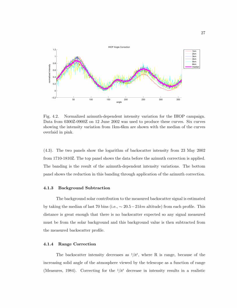
Figure (4.2) similarly shows the azimuth variation for the IHOP field campaign.
The two field campaigns occurred ∼ 2 years apart and any degradation in the HOE in
addition to changes in the instrument during transport will contribute to differences in
the azimuth variation curves.
The median of the azimuth-dependent intensity variation at each height from
∼ 600m − 6km is used as the correction curve. The correction-curve mean is scaled
to match the data mean and is then applied by dividing the data at each angle by the
appropriate correction-curve value. The results of this correction are shown in Figure
27
50 100 150 200 250 300 350−0.2
0
0.2
0.4
0.6
0.8
1
1.2IHOP Angle Correction
angle
norm
aliz
ed inte
nsity
1km
2km
3km
4km
5km
6km
median
Fig. 4.2. Normalized azimuth-dependent intensity variation for the IHOP campaign.Data from 0300Z-0900Z on 12 June 2002 was used to produce these curves. Six curvesshowing the intensity variation from 1km-6km are shown with the median of the curvesoverlaid in pink.
(4.3). The two panels show the logarithm of backscatter intensity from 23 May 2002
from 1710-1810Z. The top panel shows the data before the azimuth correction is applied.
The banding is the result of the azimuth-dependent intensity variations. The bottom
panel shows the reduction in this banding through application of the azimuth correction.
4.1.3 Background Subtraction
The background solar contribution to the measured backscatter signal is estimated
by taking the median of last 70 bins (i.e., ∼ 20.5−21km altitude) from each profile. This
distance is great enough that there is no backscatter expected so any signal measured
must be from the solar background and this background value is then subtracted from
the measured backscatter profile.
4.1.4 Range Correction
The backscatter intensity decreases as 1/R2, where R is range, because of the
increasing solid angle of the atmosphere viewed by the telescope as a function of range
(Measures, 1984). Correcting for the 1/R2 decrease in intensity results in a realistic

28
Altitude
(km
)
No Azimuth Correction − IHOP_052302b
17:20 17:30 17:40 17:50 18:00 18:100
1
2
3
4
log(I
)
−7
−6
−5
−4
−3
−2
−1
0
Time (UTC)
Altitu
de (
km
)
Azimuth Correction
17:20 17:30 17:40 17:50 18:00 18:100
1
2
3
4
log(I
)
−15
−10
−5
0
Fig. 4.3. A quicklook image showing the effect of the azimuth angle correction. Thetop panel shows the original data from 23 May 2002 from 1710-1810Z with only the de-tector correction applied. The azimuth-dependent intensity variation displays as verticalbanding in the image. The bottom panel shows the same data period with the azimuthcorrection applied. Both panels are displayed as the logarithm of the intensity.
aerosol backscatter intensity profile but also has the negative effect of amplifying any
noise present in the data. This correction is, therefore, applied after filtering the data
but prior to estimating zi.
4.1.5 Cloud Mask
Backscatter from clouds results in very strong intensity gradients in aerosol backscat-
ter data with intensities that are often one or two orders of magnitude greater than the
backscatter intensity of the CBL and, because the clouds are often optically thick, ex-
tinguish the laser energy before the actual cloud top is reached. CBL capping clouds are
considered to be part of the CBL and cloud top, whether it is real or apparent, presents a
well defined transition zone for the CBL estimators to detect. However, elevated clouds,
having the same strong cloud-top transition zone, can result in erroneous estimates of zi.
Several methods of detecting clouds in lidar backscatter data are available (Clothiaux

29
et al., 1998; Mao et al., 2011) but the method detailed by Wang and Sassen (2001) was,
for its simplicity, selected for development of a cloud-mask algorithm where each profile
is analyzed to determine if a cloud is present using
T =Ppeak
Pbase(4.1)
where Ppeak is the peak signal intensity and Pbase is the median signal intensity. Wang
and Sassen (2001) determined that a value of T > 4 indicates the presence of a cloud
with a 0.355µm lidar but, for the HARLIE lidar, operating at 1.064µm, a value of
T > 80 indicates the presence of a cloud. If a cloud is present, the profile is searched
for sequences of ≥ 5 points of increasing backscatter intensity. The use of five points
effectively prevents noise from being marked as a cloud. The first point of each sequence
is set as cloud base and the first point where the intensity returns to cloud-base intensity
is set as cloud top. Finally, using the mean and standard deviation of intensity from 15
points below cloud base, the intensity values between cloud base and top are replaced.
When CBL capping cloud signals are removed the range bins are replaced with CBL
intensity and noise values which will maintain the step at cloud top and when elevated
cloud signals are removed the range bins are replaced with FA intensity and noise values
which should minimize the step at cloud top. However, the backscatter values above a
cloud are always lower than intensities below the cloud because of signal extinction by
the cloud so a step at cloud top can never be totally eliminated.
4.1.6 Gap Detection
The scanning operation of HARLIE results in times when the lidar is pointed
towards the sun. The strong intensity of the sun causes the lidar detector to become
overwhelmed and the signal drops to near zero creating gaps in the data that appear as
edges to several of the CBL estimators. A gap detector was developed to fill the gaps
that uses the background signal values to mark the locations where gaps exist. Once the
locations of the gaps are known each gap is replaced by interpolation from the mean and
standard deviation of intensity on either side of the gap.

30
4.2 Filter Introduction
The likelihood of an estimator successfully identifying zi increases as the tran-
sition zone becomes more clearly defined and, in addition to environmental variability,
instrument noise acts to degrade the definition of the transition zone and averaging pro-
files is a common noise-reducing practice. However, it is a practice that we want to
avoid due to the reduction in data resolution and blurring of the transition zone. An-
other technique is to use noise-reducing operators, or filters, to decrease the noise in the
data without negatively impacting the features and retaining as much resolution as pos-
sible. The CNR of the data and the estimator being used drive the amount of necessary
filtering so the two will be automatically matched.
Before moving forward with a discussion of the filters it is useful to determine the
resolution limit of HARLIE scanning data. The period of rotation, P , often 12s during
both WVIOP and IHOP, results in a 30◦s−1 rotation rate and 3◦ per profile. Assuming
zi = 1km the HARLIE scan cone circumscribes a circle with a circumference of 6.28km
with each lidar profile spaced ∼ 52m apart. The horizontal scale of a CBL thermal is
typically 1.5zi (Kaimal et al., 1976; Caughey and Palmer, 1979; Young, 1988) so there are
∼ 30 lidar profiles intersecting the thermal. At 3◦ per profile this translates into ∼ 90◦
per thermal with a scan time of ∼ 3s. To capture a typical CBL thermal we can average
at most 30 profiles. However, to gather more robust EZT statistics we must average
less than 30 profiles. The range resolution of HARLIE data is 30m corresponding to a
∼ 21m vertical resolution.
4.3 Filter Description
Each filter described in the following sections has at least one parameter that is
varied to control the degree of filtering performed on the image and these values are
listed in Table 4.1.

31
4.3.1 Gaussian Filter
The Gaussian filter, also known as Gaussian blur, is defined as the convolution of
a Gaussian matrix with the image (Nixon and Aguado, 2008). The Gaussian matrix is
derived from the following equation:
g(x, y, σ) =1
2πσ2e−x
2+y
2
2σ2 (4.2)
where x and y are the azimuth and range dimensions, respectively, and σ is the standard
deviation of the Gaussian distribution. Each pixel in the new image is a weighted average
of the pixels in the neighborhood. The Gaussian filter is considered to be the workhorse
low-pass filter in image processing and will establish the baseline performance of all of
the filters.
4.3.2 Median Filter
The median filter creates a new image by replacing each pixel of the original
image by the median of values in a neighborhood and is often used to remove salt and
pepper noise because it is not as susceptible to outliers as the Gaussian filter (Lim, 1990).
While not salt and pepper in character, the noise present in lidar data does exhibit similar
random behavior so the median filter should perform relatively well. The neighborhood
of points need not be symmetric allowing for different amounts of smoothing in range
and azimuth with the lidar data.
4.3.3 Wiener Filter
Adaptive filters adjust to the features or local statistics of the image and the
Wiener filter is the first adaptive filter used in this analysis (Wiener, 1949; Lim, 1990).
The Wiener filter algorithm can be applied using a frequency or pixel-basis, the latter is
used here. The local mean and variance in an m× n neighborhood around each pixel in
image Io is estimated by

32
µ =1
m ∗ n∑m×n
Io(x, y), (4.3)
and
σ2 =1
m ∗ n∑m×n
I2o(x, y)− µ2. (4.4)
A new filtered image In is created using
In(x, y) = µ+σ2 − ν2
σ2(Io(x, y)− µ). (4.5)
The image noise variance, ν, is estimated by taking the mean of all the local variances.
Image noise should exhibit high levels of variance because it is uncorrelated in altitude
and between profiles and, conversely, the CBL should exhibit less variance. For this
reason the Wiener filter was chosen and is expected to perform relatively well. One
concern is the fact the noise still exists within the transition zone gradient causing
undesirable smoothing in this region.
4.3.4 Anisotropic Scalar Diffusion
Anisotropic scalar diffusion (SDIFF), also known as Perona-Malik diffusion (Per-
ona and Malik, 1990), is another type of adaptive filtering. It is an iterative filter that
generates a series of increasingly smoothed images with the amount of smoothing at
each pixel being controlled by the local intensity gradients around the pixel. It is loosely
related to the concept of thermal diffusion with a variable diffusion coefficient controlled
by the local image gradients. If a pixel lies near an edge the local gradients will be strong
and the smoothing operator, a Gaussian filter, will be weighted lower preserving the edge.
Conversely, if the local gradients are weak Gaussian filter weighting is increased, increas-
ing the smoothing. As the scale-space of images are generated the reduced smoothing
near edges will preserve and enhance them relative to the featureless regions. All of
the CBL estimators respond to the transition-zone gradient, but because transition-zone
gradient is essentially a diffuse edge, the SDIFF filter is expected to perform well.

33
4.3.5 Speckle Reducing Anisotropic Diffusion
Synthetic-aperture radar (SAR) and ultrasound images frequently contain speckle
noise caused by an interference pattern from scatterers smaller than the resolution of the
sensing wavelength. Speckle noise is multiplicative and, much like the additive instru-
ment noise in lidar data, can obscure features in the data. Speckle-reducing anisotropic
diffusion (SRAD) is an extension of PM diffusion tailored to reduce multiplicative noise
in images (Yu and Acton, 2002). Like SDIFF diffusion, SRAD is edge preserving but
adds a response to the local coefficient of variation in an effort to remove speckle noise.
The assumption here is that the additive noise in the lidar data is similar enough to the
multiplicative noise in SAR data for the filter to work well.
Filter Parameters
Filter Parameter Values
Gaussian
σ 2,4
x 1,3,5,7
y 1,3,5,7
Medianx 1,3,5,7
y 1,3,5,7
Wienerx 3,5,7
y 3,5,7
SDIFF num iter 1,2,3,4,5,10,15,20,30
SRADλ 0.1,0.5
num iter 20,50
Table 4.1. The parameters and the range for each of the five filters evaluated in this
study.

34
4.4 Filter Evaluation
4.4.1 Idealized Profile Optimization
An idealized profile, as detailed in Section 3.5.1, is fit to the measured aerosol
backscatter profile using a multidimensional minimization process. Recall that one of
the parameters of the idealized profile is the transition zone thickness and this value
can be used to assess the impact of the filter on the data. A genetic algorithm (GA)
(Haupt and Haupt, 2004) is used to optimize all four of the parameters to minimize the
difference between the idealized and actual lidar backscatter profiles and the result of
one of the optimizations is shown in Figure 4.4.
0 0.2 0.4 0.6 0.8 10
0.5
1
1.5
2
2.5
3
3.5
4
4.5
normalized intensity
altitu
de
(km
)
Fig. 4.4. The idealized-backscatter profile (red line) fit to an aerosol-backscatter profile(black line).
It was found that using the near-range correction, described in Section 3.5.1,
on the idealized profile reduced the performance of the GA optimization because the
inclusion of the additional parameter gave the idealized profile too much flexibility and
it tended to not lock onto zi. Therefore, the original idealized profile, as shown in Figure
3.8, is used to evaluate the filters.

35
4.4.2 Contrast-to-Noise Ratio
Prior to evaluating the filters a performance metric must be established and one
applicable measure of data quality is contrast-to-noise ratio (CNR) defined by Demehri
et al. (2012) as
CNR =|BCBL −BFA|(σ2CBL
− σ2FA
2
)1/2
(4.6)
where BCBL and BFA are the mean backscatter values in the CBL and FA, respectively,
σCBL and σFA are the standard deviation in the backscatter signal in the CBL and FA,
respectively. The values for BCBL and BFA for (4.6) are obtained from the idealized-
profile fit to the profile being evaluated. CNR is chosen over signal-to-noise ratio (SNR)
because we are interested in the contrast between the CBL and free atmosphere (FA)
and not the absolute signal level in the CBL. The filter will, ideally, increase the CNR
while minimally increasing the transition zone thickness (TZT).
4.4.3 Filter Evaluation Method
The five filters described in Section 4.3 are applied to the data over the range
of parameters, shown in Table 4.1, for each filter. We now have a measure of both the
contrast between the CBL and FA and the sharpness of the transition zone and the
combination of the two will allow us to evaluate the filters. Figure 4.5 shows the CNR
vs TZT for the well-defined development case on 2 June 2002. The black dot marks the
CNR and TZT for the unfiltered data and the desired behavior is for the filter results to
move to the upper left, which a majority of the points do in this case.

36
140 160 180 200 220 240 260 280 300 3201
2
3
4
5
6
7
TZT (m)
CN
R
IHOP_061102b
rawgaussmedian
WienerSdiffSRAD
Fig. 4.5. The transition zone thickness (TZT) vs. contrast-to-noise ratio (CNR) for
five filters from 11 June 2002 during the IHOP field campaign (Well-defined CBL). The
filters are as follows: Gauss=2D Gaussian; Median=2D Median; Wiener=2D Wiener;
Sdiff=2D anisotropic scalar diffusion; SRAD=Speckle Reducing Anisotropic Diffusion.
Application of a filter will, ideally, decrease TZT and increase CNR.
The goal is to select one filter that performs well, although not necessarily the
best, in each of the development periods.
4.5 Image Enhancement
Another method of increasing the contrast between the CBL and FA is through
the application of image enhancement algorithms. These algorithms manipulate the
distribution of image intensities reducing the influence of extreme values (e.g., noise
spikes, cloud backscatter) making subtle features visible.

37
4.5.1 Contrast Stretching
The aerosol backscatter data covers a wide range of intensities making direct com-
parisons between filter results difficult so it is useful to scale the filtered data results so
that they cover the same range. Constrast stretching, sometimes called intensity nor-
malization or histogram stretching (Gonzalez and Woods, 2008), is a method of scaling
the intensity values between 0 and 1 using
In =Io −minmax−min
. (4.7)
Here, Io is the original image and min and max are the minimum and maximum
intensities, respectively. This process, as the name implies, stretches the contrast between
intensities making features easier to discern (Figure 4.6 (left)). This method does not
alter the shape of the histogram and only changes the overall range of values (Figure 4.6
(right)).
time (UTC)
altitude (
km
)
23:18:41 23:18:49 23:18:57 23:19:05 23:19:13 23:19:21
0.5
1
1.5
2
2.5
3
3.5
4
0
0.1
0.2
0.3
0.4
0.5
0.6
0.7
0.8
0.9
1
0 0.2 0.4 0.6 0.8 10
200
400
600
800
1000
1200
1400
1600
1800
Intensity
Counts
Fig. 4.6. Left: Aerosol-backscatter image showing the results of contrast stretching.
Right: Histogram of image intensities with a range from 0 to 1.
4.5.2 Histogram Normalization
If the image histogram is dominated by a narrow set of intensities, occurring
when lidar data has large amounts of noise or clouds, other features may be hard to
detect. Histogram normalization is used to redistribute the intensity values of an image

38
by setting the lowest and highest 1% of the intensities to 0 and 1, respectively. This
effectively spreads the distribution of intensities over a wider range (Figure 4.7 (right))
making lower-contrast features easier to detect (Figure 4.7 (left)).
time (UTC)
altitude (
km
)
23:18:41 23:18:49 23:18:57 23:19:05 23:19:13 23:19:21
0.5
1
1.5
2
2.5
3
3.5
4
0
0.1
0.2
0.3
0.4
0.5
0.6
0.7
0.8
0.9
1
0 0.2 0.4 0.6 0.8 10
100
200
300
400
500
600
700
800
Intensity
Counts
Fig. 4.7. Left: Aerosol-backscatter image showing the results of histogram normaliza-
tion. Right: Histogram of image intensities after histogram normalization.
4.5.3 Histogram Equalization
Histogram equalization is used to enhance the contrast of an image by distributing
image intensities over all possible values. It is especially useful when the image intensities
are grouped over a small range of possible intensity values (Figure 4.8 (left)). Histogram
equalization produces an image with a flatter intensity histogram as seen in Figure 4.8
(right).

39
time (UTC)
altitude (
km
)
23:18:41 23:18:49 23:18:57 23:19:05 23:19:13 23:19:21
0.5
1
1.5
2
2.5
3
3.5
4
0
0.1
0.2
0.3
0.4
0.5
0.6
0.7
0.8
0.9
1
0 0.2 0.4 0.6 0.8 10
200
400
600
800
1000
1200
1400
1600
Intensity
Counts
Fig. 4.8. Left: Aerosol-backscatter image showing the results of histogram normaliza-
tion. Right: Histogram of image intensities after histogram equalization.

40
Chapter 5
CBL Depth Estimation Methods
5.1 Radiosonde Estimation of CBL Depth
Estimates of zi from radiosonde profiles provide a snapshot of the CBL depth
but this estimate of zi cannot be compared directly to lidar-derived zi estimates because
the two instruments rarely measure the same location. Radiosonde measurements do,
however, provide another independent estimate of zi in the vicinity of the lidar. Hen-
nemuth and Lammert (2006) found that the radiosonde derived zi estimates fall within
the hourly standard deviation of lidar derived zi and it is expected that the radiosonde
estimates of zi will fall within the range of zi estimates from HARLIE data.
Estimates of zi from aerosol backscatter lidar data are typically higher than es-
timated from potential temperature profiles (Coulter, 1979; Seibert et al., 2000). The
two instruments are measuring different properties of the atmosphere with the height
where the radiosonde potential-temperature profile begins to increase is selected as zi
and the lidar measuring the aerosol distribution. Aerosol-laden thermals will often pen-
etrate into the capping inversion and can deposit aerosols within the inversion resulting
in backscatter from levels above the radiosonde-derived zi. Coulter (1979) found up to
150m differences between radiosonde and aerosol lidar backscatter derived estimates of
zi.
5.2 One-Dimensional Methods
CBL depth is traditionally estimated from lidar backscatter data on a per-profile
basis (i.e., in one dimension) and, as mentioned in the introduction, some degree of av-
eraging is usually required to sufficiently reduce the noise to a level where these methods
will accurately estimate zi. However, these methods will still be evaluated in this study.

41
This section will describe the most commonly employed methods for estimating zi from
aerosol lidar data.
5.2.1 Derivatives
The most common technique for estimating zi from aerosol lidar data is to take
the first derivative of the backscatter profile with respect to altitude (Boers et al., 1984;
Stull, 1988; Nelson et al., 1989; Menut et al., 1999).
zGM = min
[∂PRSC
∂z
](5.1)
The minimum of (5.1) indicates the location of zi. Two other techniques, the
second derivative with respect to altitude (5.2) and the first derivative of the logarithm
of the data with respect to altitude (5.3), are also evaluated (Sicard et al., 2006).
zipm = min
[∂2PRCS
∂z2
](5.2) zlgm = min
[∂ln(PRCS)
∂z
](5.3)
Ideally the transition-zone gradient is the strongest gradient present in the profile
and these methods work well. However, as described in previous section, if noise is
present these methods can identify a noise-spike as zi.
5.2.2 Edge Detection
Eichinger et al. (2005) employed an edge detection technique developed by Davies
(1992) for use with digital images (5.4). The technique responds to inflection points in
the profile. The authors extend the range of the derivatives to 20 points on either side
of the point of interest to minimize the effects of noise.
zed = min
∣∣∣∣∂2PRSC/∂z2
∂PRSC/∂z
∣∣∣∣ (5.4)
5.2.3 Haar Wavelet
Davis et al. (1997); Cohn and Angevine (2000); Davis et al. (2000); Brooks (2003)
describe the technique where a Haar wavelet (step function) is convolved with the lidar

42
profile. The Haar wavelet is defined as
h
(z − ba
)=
+1 : b− a
2 ≤ z ≤ b
−1 : b ≤ z ≤ b+ a2
0 : elsewhere,
(5.5)
where z is altitude, a is the dilation, and b is the translation. The covariance transform
of the Haar function with the backscatter profile is
Wf (a, b) = PRSC ∗h =1
a
∫zt
zb
PRSCh
(z − ba
)dz. (5.6)
One of the benefits of this approach is that the parameters of the wavelet, dilation
and translation, can be adjusted to minimize the effects of noise without extensively
blurring the data. As these parameters are adjusted a common peak at zi is revealed.
The authors adjusted the parameters of the wavelet searching for the maximum wavelet
variance indicating the scale of the dominant structure in the CBL.
5.2.4 Idealized Profile
The idealized profile method, introduced conceptually in section 3.5.1 as a cus-
tomized filter evaluator, is also a robust CBL depth estimator because it uses the entire
lidar backscatter profile instead of a few select points to estimate zi.
5.3 Two-Dimensional Methods
Image processing techniques have been developed for a wide range of applications
(Nixon and Aguado, 2008) including computer vision and medical imagery feature ex-
traction. The following sections outline a selection of techniques that are expected to
be successful in detecting zi in lidar data. Each technique is tuned and, if necessary,
modified to produce a zi estimator.
A common challenge with all of the following techniques is the fact that the
transition zone is rarely a sharp edge. There are often fairly well-defined transition zone

43
gradients mixed with ill-defined gradients and the expectation is that the response of the
estimators to the well-defined transition zones will assist in the detection neighboring
ill-defined transition zones.
5.3.1 Morphological Operators
Mathematical morphology is a technique based on set theory for examining fea-
tures in images (Gonzalez and Woods, 2008). A structural element, which can have any
shape as long as it is smaller than the image being processed, is translated over the image,
pixel by pixel, and each pixel is replaced based on the operation being performed. For
example, in this study, erosion and dilation are use to simplify the aerosol-backscatter
images. With dilation, the pixels covered by the structural element are set to their maxi-
mum pixel intensity and this process acts to expand the features in an image. Conversely,
erosion replaces all of the pixels, covered by the structural element, by their minimum
pixel value acting to reduce features in an image.
Dilation followed by erosion is called image closing and acts to fill in dips or holes
in an image and erosion followed by dilation is called image opening and is used to remove
intensity peaks in an image. The image is converted to a binary image, after opening
and closing, using the method described by Otsu (1979) and the edges within binary
image are found using the bwlabel function in Matlab based on Haralick and Shapiro
(1992).
5.3.2 Edge Detection
There are a wide range of edge detection techniques available including Sobel,
Canny, and Marr-Hildreth (Duda and Hart, 1973; Canny, 1986; Withey et al., 2009).
Most of the edge-detection techniques are essentially one- or two-dimensional derivatives.
The Canny edge detector is one of the most widely used and was therefore selected for
this analysis. The first step is to apply a Gaussian smoother to the image to reduce
the influence of isolated noise spikes. Next the magnitude and direction of the image
gradients are found with the directions of image gradients being rounded to represent
vertical, horizontal, and two diagonal gradients. The larger the intensity of the gradient

44
the more likely it represents an actual edge in the image and these edges, in combination
with a high threshold, form the starting points for finding the actual edges. Then, using
the directional gradients, the actual edges are traced using a low threshold and the end
result is a binary image with all of the image edges marked.
The standard Canny edge detector did not detect zi properly because of the noise,
even after filtering, that was present in the image. Therefore, a series of Canny edge
detectors, with increasing Gaussian smoothing (i.e., σ =4, 6, 8, 10, and 12), was applied
to the aerosol backscatter image creating a scale-space (Perona and Malik, 1990) of
images representing features of increasing size. The CBL, being a large scale feature,
will be present in all of the scale-space images but with much less detail when σ is large.
Recall that the Canny edge detector returns a binary image so the edges found at all
scales are summed and the result is thresholded to find the edges that are common at
all scales.
5.3.3 Active Contours
Also known as snakes, active contours are an energy minimization technique (Ter-
zopoulos et al., 1987; Kass et al., 1988; Staib and Duncan, 1996; Unser, 1999; Brigger
et al., 2000). Parikh and Parikh (2002) employed a combination of edge detection and
active contours to extract CBL depth from lidar data. The response of a contour to a
feature is a balance between the dynamics of the contour and the features in the image.
The initial contour is rectangular in shape and composed of a series of points. The
contour begins to expand because of a defined balloon force and the individual points
are attracted to intensity gradients in the image. Contour points that settle on strong
gradients will influence adjacent points because of the constraints imposed by the con-
tour dynamics (e.g., forces that resist stretching and bending) so the influenced points
are more likely to settle on the correct intensity gradient, even if it is ill-defined, as they
use information from nearby profiles and contour dynamics.

45
5.3.4 k-Means Clustering
K-means clustering partitions the data into k clusters by minimizing the mean-
squared error (MSE) between the points and the cluster centroids (Seber, 1984). It is
an iterative process, alternating between assignment and update steps, that begins by
assigning all the points to the nearest randomly-positioned centroid. Next, the centroids
are updated based on the new point assignments. The points are assigned to the centroid
that results in the lowest MSE and the centroid is updated again. This process continues
until no new assignments are made. The clustered data points form a binary image and
the boundary between the clusters is found using similar methods as the morphological
operators in Section 5.3.1.
5.4 Location of zi within the Transition Zone
Section 1.1 provided a discussion on the definition of the CBL top and how there is
no universally accepted definition. In addition to aerosols deposited by earlier thermals,
new aerosols are constantly being deposited by new thermals while FA air is being mixed
downward (Deardorff et al., 1980; Davis et al., 1997; Grabon et al., 2010). As a result of
this complex mixing the CBL does not have a distinct, sharply defined, top, rather, the
CBL top forms a transition zone (Brooks, 2003) and the generally accepted location of
zi is the center of the transition zone. Although the traditional bottom of the inversion
definition of zi corresponds to the bottom of the transition zone, each of the estimators,
both 1- and 2-D, will, for a given aerosol backscatter profile, select a slightly different
location for zi, within the transition zone, driven by the design of the estimator.
5.5 Human Estimation of CBL Depth
Human estimation of CBL depth provides a benchmark for evaluation of the CBL
estimators described above. A human estimating zi from an aerosol-backscatter image
will utilize the spatial distribution of intensities in combination with an understanding
of CBL physics. A graphical user interface (GUI) was developed in Matlab to facilitate
the human evaluation of aerosol-backscatter images. The users are presented with an

46
image, either filtered or unfiltered, where they can manually select the location of zi with
a total of 17 periods evaluated by the users. The corresponding radiosonde potential-
temperature profile is also presented to aid in the selection of zi. The GUI instructions
are included in the Appendix. A consensus of the human estimates is necessary for
comparison with the automated estimators. The group of human estimators in this
study is comprised of the author’s faculty committee. All of them possess knowledge,
some extensive, of CBL structure and dynamics and, because no outlying estimates are
expected, the mean of their estimates will be used as the consensus for comparison with
the automated methods.
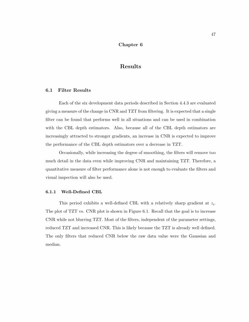
47
Chapter 6
Results
6.1 Filter Results
Each of the six development data periods described in Section 4.4.3 are evaluated
giving a measure of the change in CNR and TZT from filtering. It is expected that a single
filter can be found that performs well in all situations and can be used in combination
with the CBL depth estimators. Also, because all of the CBL depth estimators are
increasingly attracted to stronger gradients, an increase in CNR is expected to improve
the performance of the CBL depth estimators over a decrease in TZT.
Occasionally, while increasing the degree of smoothing, the filters will remove too
much detail in the data even while improving CNR and maintaining TZT. Therefore, a
quantitative measure of filter performance alone is not enough to evaluate the filters and
visual inspection will also be used.
6.1.1 Well-Defined CBL
This period exhibits a well-defined CBL with a relatively sharp gradient at zi.
The plot of TZT vs. CNR plot is shown in Figure 6.1. Recall that the goal is to increase
CNR while not blurring TZT. Most of the filters, independent of the parameter settings,
reduced TZT and increased CNR. This is likely because the TZT is already well defined.
The only filters that reduced CNR below the raw data value were the Gaussian and
median.

48
140 160 180 200 220 240 260 280 300 3201
2
3
4
5
6
7
TZT (m)
CN
R
IHOP_061102b
rawgaussmedian
WienerSdiffSRAD
Fig. 6.1. The transition zone thickness (TZT) vs. contrast-to-noise ratio (CNR) for
five filters from 11 June 2002 during the IHOP field campaign (Well-defined CBL). The
filters are as follows: Gauss=2D Gaussian; Median=2D Median; Wiener=2D Wiener;
Sdiff=2D anisotropic scalar diffusion; SRAD=Speckle Reducing Anisotropic Diffusion.
6.1.2 Ill-Defined CBL
The results from this period show more variability than the previous case (Figure
6.2). The transition zone thickness is larger, 390m vs. 310m. The Gaussian and median
filters displayed the widest range of TZT change, but they both, at times, decreased
CNR and increased TZT. The is no standout filter in this period but the Wiener filter
does perform consistently well.

49
150 200 250 300 350 400 4501
1.5
2
2.5
3
3.5
4
4.5
TZT (m)
CN
R
IHOP_060802
rawgaussmedian
WienerSdiffSRAD
Fig. 6.2. The transition zone thickness (TZT) vs. contrast-to-noise ratio (CNR) for
five filters from 11 June 2002 during the IHOP field campaign (Ill-defined CBL). The
filters are as follows: Gauss=2D Gaussian; Median=2D Median; Wiener=2D Wiener;
Sdiff=2D anisotropic scalar diffusion; SRAD=Speckle Reducing Anisotropic Diffusion.
6.1.3 Layers
This period has the CBL growing within a residual layer from the previous day
(Figure 3.5 (left)) and the TZT vs. CNR plot is shown in Figure 6.3. Here, the results
are grouped together more than the ill-defined CBL period. The Wiener and SDIFF
filters both tend to increase CNR while keeping TZT at ∼ 220m.

50
180 200 220 240 260 280 300 3201
1.5
2
2.5
3
3.5
4
4.5
5
TZT (m)
CN
R
IHOP_060102
rawgaussmedian
WienerSdiffSRAD
Fig. 6.3. The entrainment zone thickness (EZT) vs. contrast-to-noise ratio (CNR)
for five filters from 01 June 2002 during the IHOP field campaign (Layers). The filters
are as follows: Gauss=2D Gaussian; Median=2D Median; Wiener=2D Wiener; PM=2D
Perona Malik scalar diffusion; Tdiff=2D tensor diffusion.
6.1.4 Clouds
This period features an elevated cloud layer that tests the performance of the
cloud-mask routine. All of the filters tended to decrease TZT and increase CNR, as shown
in Figure 6.4, but the Gaussian and median filters exhibiting a wider range of results
compared to the other filters. The SRAD filter did increase CNR, in one realization,
higher than the other filters.

51
140 160 180 200 220 240 260 280 300 320 3401
1.5
2
2.5
3
3.5
4
TZT (m)
CN
R
WVIOP_100600a
rawgaussmedian
WienerSdiffSRAD
Fig. 6.4. The transition zone thickness (TZT) vs. contrast-to-noise ratio (CNR) for
five filters from 11 June 2002 during the IHOP field campaign (Clouds). The filters are
as follows: Gauss=2D Gaussian; Median=2D Median; Wiener=2D Wiener; Sdiff=2D
anisotropic scalar diffusion; SRAD=Speckle Reducing Anisotropic Diffusion.
6.1.5 Data Gaps
This period’s results, shown in Figure 6.5, exhibit a wider range of CNR values
than the other periods. In most realizations TZT is decreased but there is often a
decrease in CNR values. The Wiener, SDIFF, and SRAD filters performed equally well
with a slightly greater increase in CNR with the SRAD filter.

52
100 150 200 250 300 350 400 450
0.8
1
1.2
1.4
1.6
1.8
2
TZT (m)
CN
R
IHOP_060202
rawgaussmedian
WienerSdiffSRAD
Fig. 6.5. The transition zone thickness (TZT) vs. contrast-to-noise ratio (CNR) for
five filters from 11 June 2002 during the IHOP field campaign (Gaps). The filters are
as follows: Gauss=2D Gaussian; Median=2D Median; Wiener=2D Wiener; Sdiff=2D
anisotropic scalar diffusion; SRAD=Speckle Reducing Anisotropic Diffusion.
6.1.6 Synthetic Data
This period’s results reveal an almost textbook behavior with a decrease in TZT
and increase in CNR with every filter realization (Figure 6.6). The Wiener filter results
are relatively grouped in the upper right of the raw data values.

53
315 320 325 330 335 340 345 350 3554
6
8
10
12
14
16
TZT (m)
CN
R
synthetic
rawgaussmedian
WienerSdiffSRAD
Fig. 6.6. The transition zone thickness (TZT) vs. contrast-to-noise ratio (CNR) for
five filters from 11 June 2002 during the IHOP field campaign. The filters are as follows:
Gauss=2D Gaussian; Median=2D Median; Wiener=2D Wiener; Sdiff=2D anisotropic
scalar diffusion; SRAD=Speckle Reducing Anisotropic Diffusion.
6.1.7 Filter Discussion and Selection
The Gaussian and median filters produced mixed results but never performed
as well as the other three filters. This is not surprising because these filters operate
uniformly over the entire image. The remaining three filters; Wiener, SDIFF, and SRAD,
performed similarly over the development periods with the Wiener tending to have the
greater increase in CNR value and filter rarely decreased CNR.
However, visual inspection of the filtered data reveals undesirable behavior in
some of these filters. Figure (6.7) shows small segments of filtered data from 11 June
2002 (i.e., the well-defined CBL period) for the Wiener, SDIFF, and SRAD filters. The
blue line represents a single aerosol backscatter profile (i.e., profile #50). As mentioned
above, quantitatively, the Wiener filter consistently outperformed the other filters. The

54
higher backscatter CBL intensity is clearly visible and the transition-zone gradient is
well defined. However, crosshatch artifacts can be seen in the image and, even though
the filter is removing noise from the original data, it is introducing new noise in the form
of these artifacts.
profile20 40 60 80 100
0.5
1
1.5
2
2.5
3
3.5
40 0.5 1
0.5
1
1.5
2
2.5
3
3.5
4
Wiener
altitu
de
(km
)
profile20 40 60 80 100
0.5
1
1.5
2
2.5
3
3.5
40 0.5 1
0.5
1
1.5
2
2.5
3
3.5
4
SDIFF
profile20 40 60 80 100
0.5
1
1.5
2
2.5
3
3.5
40 0.5 1
0.5
1
1.5
2
2.5
3
3.5
4
SRAD
Fig. 6.7. Segments of aerosol-backscatter intensity images showing the effects of the
Wiener (left), SDIFF (middle), and SRAD (right) filters. The blue line is a single aerosol-
backscatter profile (i.e., profile #50). The Wiener filter introduces artifacts, and noise,
in the image. The SDIFF filter smoothly filters the data while keeping the transition
zone clearly defined ∼ 1.2km. The SRAD filter does not maintain the contrast between
the CBL and FA.
The SDIFF filter also has a clearly defined CBL and transition-zone gradient
but the noise, visible in the upper portion of the profile, is gradually smoothed. The
profile for the SRAD filter shows a much less contrast between the CBL and FA than
the other filters. Also, a blank region is visible in the upper right of the image and
this loss of data was observed when isolated pixels with backscatter intensities several
orders of magnitude greater than the surrounding pixels were present. These hot pixels

55
may be a result of portions of cloud-backscatter pixels passing through the cloud mask
algorithm. Also, the SRAD filter requires a selection of pixels to estimate the speckle
statistics in the image and it is found that the performance of the filter is very sensitive
to the selection of these pixels making it unreliable for this study.
Overall, the SDIFF filter performs well by decreasing TZT and increasing CNR
and it is shown to be capable of a wide range of smoothing degrees by simply adjusting
a single parameter; the number of iterations. It has acceptable smoothing behavior as
shown in Figure (6.7) and, therefore, the SDIFF filter will be used with the CBL depth
estimators in the remainder of this study.
6.2 CBL Estimator Discussion
Each estimator detailed in Sections 5.2 and 5.3 is applied to the raw and SDIFF-
filtered data over the number of iterations listed in Table 4.1 for each development period.
None of the one-dimensional methods, with the exception of the idealized profile, perform
reliably on any of the development periods. This result is expected due to, as mentioned
in Section 5.2, the application of the one-dimensional estimators to individual profiles
and the degree of noise, even with application of the SDIFF filter, present in the data.
For example, Figure 6.8 shows the results of the first-derivative estimator for the well-
defined CBL period (e.g., 11 June 2002). By definition, this estimator selects the largest
gradient in each profile as zi and, frequently, the largest gradient occurs in the noise near
the top of the profile.

56
time (UTC)
altitude (
km
)
11 June 2002 − 1st Deriv. Estimator
16:35:29 16:35:39 16:35:49 16:35:59 16:36:09 16:36:20
0.5
1
1.5
2
2.5
3
3.5
4raw1234510152030
Fig. 6.8. Aerosol-backscatter image showing the performance of the first-derivative CBL
depth estimator. The colors represent the number of iterations of the SDIFF filter used
with the estimator.
Another example of the inadequate performance of the one-dimensional methods
is shown in Figure 6.9 for the wavelet estimator. Even with the built-in scale-space
nature of the wavelet method the noise dominates individual profiles.
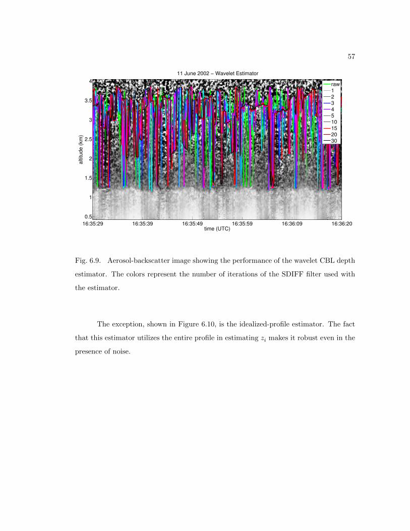
57
time (UTC)
altitude (
km
)
11 June 2002 − Wavelet Estimator
16:35:29 16:35:39 16:35:49 16:35:59 16:36:09 16:36:20
0.5
1
1.5
2
2.5
3
3.5
4raw1234510152030
Fig. 6.9. Aerosol-backscatter image showing the performance of the wavelet CBL depth
estimator. The colors represent the number of iterations of the SDIFF filter used with
the estimator.
The exception, shown in Figure 6.10, is the idealized-profile estimator. The fact
that this estimator utilizes the entire profile in estimating zi makes it robust even in the
presence of noise.

58
time (UTC)
altitude (
km
)
11 June 2002 − Idealized−Profile Estimator
16:35:29 16:35:39 16:35:49 16:35:59 16:36:09 16:36:20
0.5
1
1.5
2
2.5
3
3.5
4raw1234510152030
Fig. 6.10. Aerosol-backscatter image showing the performance of the idealized-profile
CBL depth estimator. The colors represent the number of iterations of the SDIFF filter
used with the estimator.
An example of a two-dimensional estimator, the active contour, is shown in Figure
6.11. Only the two-dimensional estimators, in addition to the idealized-profile estimator,
are used in the remainder of the study. It is clear from Figure 6.11 that the performance
of the estimator depends on the number of iterations of the SDIFF filter. A method of
matching the number of iterations to the estimator is developed and described in the
next section.

59
time (UTC)
altitude (
km
)
11 June 2002 − Active−Contour Estimator
16:35:29 16:35:39 16:35:49 16:35:59 16:36:09 16:36:20
0.5
1
1.5
2
2.5
3
3.5
4raw1234510152030
Fig. 6.11. Aerosol-backscatter image showing the performance of the active-contour
CBL depth estimator. The colors represent the number of iterations of the SDIFF filter
used with the estimator.
6.3 Merging Estimates
There will be differences between estimator results because each estimator re-
sponds differently to the same transition zone gradient and these differences can be
leveraged by combining the individual estimator results into a merged result. The me-
dian of the individual estimators is used as the merged estimate. The advantage of the
median is that it is not influenced by outliers so, if a single estimator is locked onto a
feature other than the transition zone, such as an elevated aerosol layer or cloud, it won’t
negatively influence the merged estimate. However, if multiple estimators are locked onto
a feature other than zi, the merged estimate will be biased.

60
6.4 Filter-Estimator Matching
In Figure 6.11 the effects of filtering on the estimator results can be seen by the
distribution of CBL depth estimates. The higher number of iterations (e.g., 20 and
30) blur the transition zone and the active-contour settles on another feature within
the CBL. However, one of the lower number of iterations (e.g., raw, 1, 2, or 3) follows
the transition zone gradient. Therefore, it is assumed that the application an optimal
number of iterations of the SDIFF filter will provide the optimal image for each estimator
to find zi. It is also assumed that if each estimator is correctly estimating zi, the range
of estimates should be relatively small.
Because the overall CNR value and strength of the transition zone varies greatly
over the development periods, it is difficult to select a single filter iteration count for
each of the estimators. Therefore, the optimal number of iterations for each estimator
is found for each development period. The process for a single period is
1. Apply all 10 number of iterations (Table 4.1) to the aerosol-backscatter image.
2. Estimate zi in each of the 10 filtered images using the five estimators.
3. Find the iterations/estimator pairs that produce the smallest range of of estimates.
Figure 6.12 shows, for each of the six development periods, the minimum range
of the zi estimates (top panel) and the number of iterations matched to each estimator
(bottom panel) that produced the minimum range.
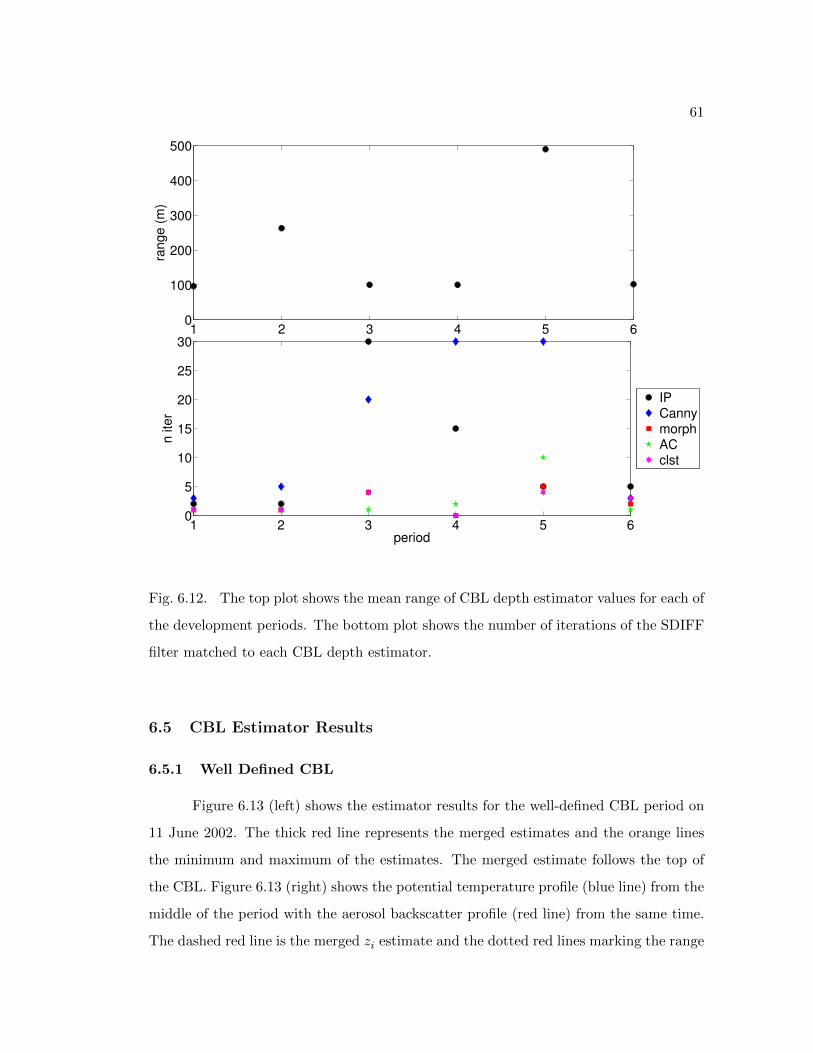
61
1 2 3 4 5 60
100
200
300
400
500ra
ng
e (
m)
1 2 3 4 5 60
5
10
15
20
25
30
period
n ite
r
IPCannymorphACclst
Fig. 6.12. The top plot shows the mean range of CBL depth estimator values for each of
the development periods. The bottom plot shows the number of iterations of the SDIFF
filter matched to each CBL depth estimator.
6.5 CBL Estimator Results
6.5.1 Well Defined CBL
Figure 6.13 (left) shows the estimator results for the well-defined CBL period on
11 June 2002. The thick red line represents the merged estimates and the orange lines
the minimum and maximum of the estimates. The merged estimate follows the top of
the CBL. Figure 6.13 (right) shows the potential temperature profile (blue line) from the
middle of the period with the aerosol backscatter profile (red line) from the same time.
The dashed red line is the merged zi estimate and the dotted red lines marking the range

62
of estimates. As mentioned in Section 5.1, there is an expected difference between the θ
profile and the zi estimate lies near the top of the potential-temperature inversion.
time (UTC)
altitu
de
(km
)
IHOP_061102b
16:35:29 16:35:39 16:35:49 16:35:59 16:36:09 16:36:20
0.5
1
1.5
2
2.5
3
3.5
4
0 0.2 0.4 0.6 0.8 1
0.5
1
1.5
2
2.5
3
3.5
4
Relative Backscatter
altitu
de
(km
)
Fig. 6.13. Left: Aerosol-backscatter image for 11 June 2002 (well-defined CBL) with
the merged CBL depth estimates (red line) and the range of the CBL depth estimators
(orange line). Right: Potential-temperature profile (blue line) and aerosol-backscatter
profile (red line), from the center of the period, and the merged CBL depth estimator
result (red dashed line).
6.5.2 Ill-Defined CBL
This period, as mentioned in Section 3.4.2, features an undulating zi that is oc-
casionally ill-defined (i.e., weak transition-zone gradient). The estimates for this period,
shown in Figure 6.14 (left), show a greater range than the previous period but the
merged estimate tends to follow the transition-zone gradient. Figure 6.14 (right) shows
the potential-temperature (blue line) and aerosol backscatter (red line) profiles for the
middle of the period. The estimator result (red dashed line) is again relatively close to
the top of the potential-temperature inversion.

63
time (UTC)
altitu
de
(km
)IHOP_060802
17:44:45 17:44:55 17:45:06 17:45:16 17:45:27 17:45:38
0.5
1
1.5
2
2.5
3
3.5
4
305 310 315 320 325
0.5
1
1.5
2
2.5
3
3.5
4
θ
altitu
de
(km
)
−0.5 0 0.5 1 1.5
0.5
1
1.5
2
2.5
3
3.5
4
relative intensity
Fig. 6.14. Left: Aerosol-backscatter image for 8 June 2002 (ill-defined CBL) with the
merged CBL depth estimates (red line) and the range of the CBL depth estimators
(orange line). Right: Potential-temperature profile (blue line) and aerosol-backscatter
profile (red line), from the center of the period, and the merged CBL depth estimator
result (red dashed line).
6.5.3 Layers
This period features several aerosol layers that can mistaken as zi. Examining
the radiosonde profile in Figure 6.15 (right) reveals several locations where the potential
temperature profile changes slope but zi is likely located at ∼ 400m and a residual layer
at ∼ 1200m. The higher intensity visible as a horizontal undulating brightness below
1km in Figure 6.15 (left) is backscatter from the CBL aerosols. Unfortunately, none of
the estimators locked onto the CBL top instead settling on the top of the residual layer.
The aerosol backscatter profile in Figure 6.15 (right) does show a very small decrease in
intensity at ∼ 1km that may indicate of zi but is is very minimal, especially compared to
the transition zone at ∼ 1.3km. In this case, even with filtering, there isn’t information
for an accurate estimate of zi.

64
time (UTC)
altitu
de
(km
)IHOP_060102
17:52:04 17:52:14 17:52:25 17:52:35 17:52:46 17:52:57
0.5
1
1.5
2
2.5
3
3.5
4
310 315 320 325
0.5
1
1.5
2
2.5
3
3.5
4
θ
altitu
de
(km
)
−0.5 0 0.5 1 1.5
0.5
1
1.5
2
2.5
3
3.5
4
relative intensity
Fig. 6.15. Left: Aerosol-backscatter image for 1 June 2002 (Layers) with the merged
CBL depth estimates (red line) and the range of the CBL depth estimators (orange line).
Right: Potential-temperature profile (blue line) and aerosol-backscatter profile (red line),
from the center of the period, and the merged CBL depth estimator result (red dashed
line).
6.5.4 Clouds
Figure 6.16 (left) shows the aerosol-backscatter image prior to application of the
cloud-mask algorithm. The intensity gradient at cloud top would have been mistaken as
zi but the results shown on Figure 6.16 (left) reveal otherwise. The algorithm, described
in Section 4.1.5, effectively removed the cloud-enhanced backscatter from the data (red
line) resulting in accurate zi estimates with a relatively narrow range. Figure 6.16
(right) shows the potential-temperature (blue line) with the dashed red line indicating the
merged CBL depth estimate. The potential-temperature inversion is relatively shallow
but the merged results lie slightly above the top of the inversion.

65
time (UTC)
altitu
de
(km
)WVIOP_100600a
17:31:40 17:31:48 17:31:56 17:32:04 17:32:12 17:32:20
0.5
1
1.5
2
2.5
3
3.5
4
280 290 300 310
0.5
1
1.5
2
2.5
3
3.5
4
θ
altitu
de
(km
)
−0.5 0 0.5 1 1.5
0.5
1
1.5
2
2.5
3
3.5
4
relative intensity
Fig. 6.16. Left: Aerosol-backscatter image for 6 October 2000 (Clouds) with the merged
CBL depth estimates (red line) and the range of the CBL depth estimators (orange line).
Right: Potential-temperature profile (blue line) and aerosol-backscatter profile (red line),
from the center of the period, and the merged CBL depth estimator result (red dashed
line).
6.5.5 Data Gaps
The gap-detection algorithm, detailed in Section 4.1.6, effectively removed the
influence of the data gaps as shown by the zi estimates in Figure 6.17 (left). The CNR
values for this period (Figure 6.5) are relatively low and the range of the CBL depth
estimates is larger than the other development periods (orange line in Figure 6.17 (left)).
However, the merged estimates tend to follow the transition zone with a few deviations
(e.g., high estimates at 17:26:42). Figure 6.17 (right) shows the merged zi estimate,
which agrees well with the aerosol backscatter profile.

66
time (UTC)
altitu
de
(km
)IHOP_060202
17:27:26 17:27:36 17:27:46 17:27:57 17:28:07 17:28:18
0.5
1
1.5
2
2.5
3
3.5
4
310 315 320 325
0.5
1
1.5
2
2.5
3
3.5
4
θ
altitu
de
(km
)
−0.5 0 0.5 1 1.5
0.5
1
1.5
2
2.5
3
3.5
4
relative intensity
Fig. 6.17. Left: Aerosol-backscatter image for 2 June 2002 (Data Gaps) with the merged
CBL depth estimates (red line) and the range of the CBL depth estimators (orange line).
Right: Potential-temperature profile (blue line) and aerosol-backscatter profile (red line),
from the center of the period, and the merged CBL depth estimator result (red dashed
line).
6.5.6 Synthetic Data
Figure 6.18 (left) shows the merged estimator results for the synthetic data period.
There are several narrow gaps in the data that attract one of the estimators but overall
the merged estimate follows the transition zone. Figure 6.18 (right) shows the aerosol-
backscatter profile from the center of the period (red line) and the merged CBL depth
estimator result (red dashed line). Figure 6.19 shows the merged estimate (red line)
and the actual zi values (green line) set when the data were generated. The RMS error
between the merged and actual zi values for the period is 56m.

67
time (UTC)
altitu
de
(km
)
synth
23:02:33 23:02:41 23:02:49 23:02:57 23:03:05 23:03:13
0.5
1
1.5
2
2.5
3
3.5
4
−0.5 0 0.5 1 1.5
0.5
1
1.5
2
2.5
3
3.5
4
altitu
de
(km
)
relative intensity
Fig. 6.18. Left: Aerosol-backscatter image for the synthetic data set with the merged
CBL depth estimates (red line) and the range of the CBL depth estimators (orange
line). Right: Aerosol-backscatter profile (red line), from the center of the period, and
the merged CBL depth estimator result (red dashed line).
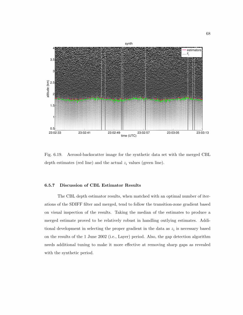
68
time (UTC)
altitude (
km
)
synth
23:02:33 23:02:41 23:02:49 23:02:57 23:03:05 23:03:13
0.5
1
1.5
2
2.5
3
3.5
4estimatorsz
i
Fig. 6.19. Aerosol-backscatter image for the synthetic data set with the merged CBL
depth estimates (red line) and the actual zi values (green line).
6.5.7 Discussion of CBL Estimator Results
The CBL depth estimator results, when matched with an optimal number of iter-
ations of the SDIFF filter and merged, tend to follow the transition-zone gradient based
on visual inspection of the results. Taking the median of the estimates to produce a
merged estimate proved to be relatively robust in handling outlying estimates. Addi-
tional development in selecting the proper gradient in the data as zi is necessary based
on the results of the 1 June 2002 (i.e., Layer) period. Also, the gap detection algorithm
needs additional tuning to make it more effective at removing sharp gaps as revealed
with the synthetic period.

69
6.6 Comparison with Human Estimates of CBL Depth
The human estimates of zi (Section 5.5) are considered to be the true zi and are
used to assess the performance of the merged-estimator results. The aerosol-backscatter
image from 4 October 2000 is shown in Figure 6.20 with the human (blue line) and
merged (red line) CBL depth estimates. For this period σhuman, the mean standard
deviation of the human estimates, is 37m, and the root mean square deviation, RMSD,
between the merged and human estimates is 65m, resulting in RMSD< 2σhuman.
time (UTC)
altitude (
km
)
WVIOP_100400
23:27:40 23:27:48 23:27:56 23:28:04 23:28:12 23:28:20
0.5
1
1.5
2
2.5
3
3.5
4estimators
human
Fig. 6.20. Aerosol-backscatter image showing the results of the human (blue line) and
merged (red line) CBL depth estimates for 4 October 2000.
Figure 6.21 shows the range of human estimates (blue area) for the same period.
Qualitatively, the merged CBL depth estimates quite often lie within the range of the
human estimates.

70
time (UTC)
altitude (
km
)
WVIOP_100400
23:27:40 23:27:48 23:27:56 23:28:04 23:28:12 23:28:20
0.5
1
1.5
2
2.5
3
3.5
4
Fig. 6.21. Aerosol-backscatter image showing the results of the human (blue line) and
merged (red line) CBL depth estimates for 4 October 2000. The light blue lines indicate
the range of human estimates for the period.
Another period, from 20 September 2000, is shown in Figure 6.22 with the human
(blue line) and merged (red line) CBL depth estimates. As with the previous period the
merged estimate captures the behavior of zi with an RMSD= 42m and σhuman = 47m.
Figure 6.23 shows that the merged CBL depth estimates lie within the range of the
human estimates a majority of the time.

71
time (UTC)
altitude (
km
)
WVIOP_092000
23:34:20 23:34:36 23:34:52 23:35:08 23:35:24 23:35:40
0.5
1
1.5
2
2.5
3
3.5
4estimators
human
Fig. 6.22. Aerosol-backscatter image showing the results of the human (blue line) and
merged (red line) CBL depth estimates for 20 September 2000.

72
time (UTC)
altitude (
km
)
WVIOP_092000
23:34:20 23:34:36 23:34:52 23:35:08 23:35:24 23:35:40
0.5
1
1.5
2
2.5
3
3.5
4
Fig. 6.23. Aerosol-backscatter image showing the results of the human (blue line) and
merged (red line) CBL depth estimates for 20 September 2000. The light blue lines
indicate the range of human estimates for the period.
For the 21 September 2000 period, the mean estimator range was 1134m and can
be seen in Figure 6.24 as the orange lines. The low zi estimate is likely from a single
estimator and taking the median of the estimates effectively excludes this outlier. The
merged CBL depth estimates tend to lie within the range of human estimates except for
a brief time at the beginning of the period (Figure 6.25). Overall, the merged estimate
accurately tracks the human estimates with RMSD= 75m and σhuman = 30m for this
period.

73
time (UTC)
altitude (
km
)
WVIOP_092100
23:28:40 23:28:48 23:28:56 23:29:04 23:29:12 23:29:20
0.5
1
1.5
2
2.5
3
3.5
4
Fig. 6.24. Aerosol-backscatter image showing the results of the human (blue line) and
merged (red line) CBL depth estimates for 21 September 2000. The orange lines indicate
the range of the CBL depth estimators.

74
time (UTC)
altitude (
km
)
WVIOP_092100
23:28:40 23:28:48 23:28:56 23:29:04 23:29:12 23:29:20
0.5
1
1.5
2
2.5
3
3.5
4
Fig. 6.25. Aerosol-backscatter image showing the results of the human (blue line) and
merged (red line) CBL depth estimates for 21 September 2000. The light blue lines
indicate the range of human estimates for the period
An example of poor merged-estimate performance is shown for the 6 October 2000
period in Figure 6.26 where RMSD= 268m and σhuman = 46m. This period shows the
difficulty in retrieving the top of the CBL as it grows within the a residual layer. There
is transition zone at ∼ 1.2km that all of the human estimates indicate as zi (Figure 6.27)
but all of the individual estimators locked onto features associated with the growing
internal CBL as indicated by the range of CBL estimators shown by the orange lines
in Figure 6.26. Examination of the radiosonde θ profile (Figure 6.28) does support
zi ≈ 1km at the time of the launch at 20:30 UTC but the human and merged estimates
are within 100m at this time. The aerosol-backscatter image is the only evidence that
the transition-zone at ∼ 1.2km is a residual layer so it cannot be concluded that the
human estimates are in error.

75
time (UTC)
altitude (
km
)
WVIOP_100600b
20:29:40 20:29:48 20:29:56 20:30:04 20:30:12 20:30:20
0.5
1
1.5
2
2.5
3
3.5
4
Fig. 6.26. Aerosol-backscatter image showing the results of the human (blue line) and
merged (red line) CBL depth estimates for 6 October 2000. The orange lines indicate
the range of the CBL depth estimators.

76
time (UTC)
altitude (
km
)
WVIOP_100600b
20:29:40 20:29:48 20:29:56 20:30:04 20:30:12 20:30:20
0.5
1
1.5
2
2.5
3
3.5
4
Fig. 6.27. Aerosol-backscatter image showing the results of the human (blue line) and
merged (red line) CBL depth estimates for 6 October 2000. The light-blue lines indicate
the range of the human CBL depth estimates.
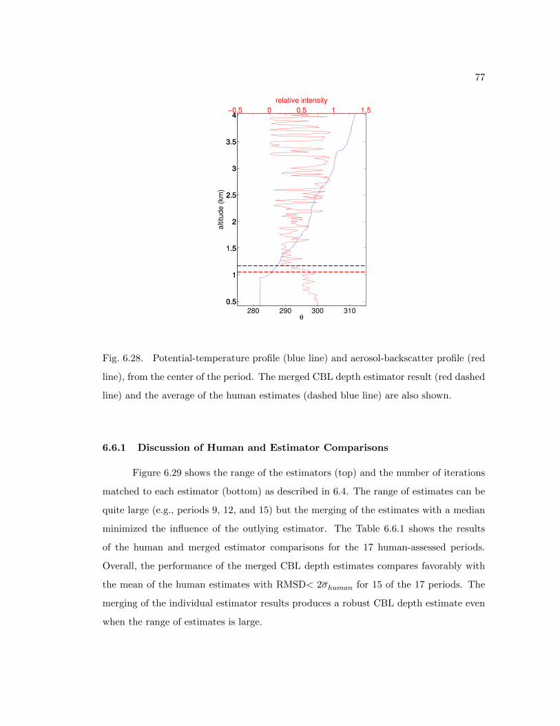
77
280 290 300 310
0.5
1
1.5
2
2.5
3
3.5
4
θ
altitude (
km
)
−0.5 0 0.5 1 1.5
0.5
1
1.5
2
2.5
3
3.5
4
relative intensity
Fig. 6.28. Potential-temperature profile (blue line) and aerosol-backscatter profile (red
line), from the center of the period. The merged CBL depth estimator result (red dashed
line) and the average of the human estimates (dashed blue line) are also shown.
6.6.1 Discussion of Human and Estimator Comparisons
Figure 6.29 shows the range of the estimators (top) and the number of iterations
matched to each estimator (bottom) as described in 6.4. The range of estimates can be
quite large (e.g., periods 9, 12, and 15) but the merging of the estimates with a median
minimized the influence of the outlying estimator. The Table 6.6.1 shows the results
of the human and merged estimator comparisons for the 17 human-assessed periods.
Overall, the performance of the merged CBL depth estimates compares favorably with
the mean of the human estimates with RMSD< 2σhuman for 15 of the 17 periods. The
merging of the individual estimator results produces a robust CBL depth estimate even
when the range of estimates is large.

78
0 2 4 6 8 10 12 14 16 180
200
400
600
800
1000
1200ra
ng
e (
m)
0 2 4 6 8 10 12 14 16 180
5
10
15
20
25
30
n ite
r
period
IPCannymorphACclst
Fig. 6.29. The top plot shows the mean range of CBL depth estimator values for each
of the periods. The bottom plot shows the number of iterations of the SDIFF filter
matched to each CBL depth estimator.
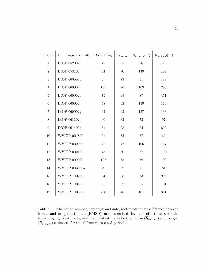
79
Period Campaign and Date RMSD (m) σhuman Rhuman(m) Rmerged(m)
1 IHOP 052802b 72 35 78 178
2 IHOP 053102 44 70 149 108
3 IHOP 060502b 37 23 51 112
4 IHOP 060802 101 76 169 263
5 IHOP 060902c 75 39 87 451
6 IHOP 060902f 58 62 139 119
7 IHOP 060902g 92 63 137 133
8 IHOP 061102b 60 33 73 97
9 IHOP 061402a 31 28 64 692
10 WVIOP 091800 51 35 77 69
11 WVIOP 092000 42 47 106 167
12 WVIOP 092100 75 30 67 1134
13 WVIOP 092900 122 35 79 190
14 WVIOP 093000a 49 32 71 81
15 WVIOP 100200 84 28 63 995
16 WVIOP 100400 65 37 85 101
17 WVIOP 100600b 268 46 101 381
Table 6.1. The period number, campaign and date, root mean square difference betweenhuman and merged estimates (RMSD), mean standard deviation of estimates for thehuman (σhuman) estimates, mean range of estimates for the human (Rhuman) and merged(Rmerged) estimates for the 17 human-assessed periods.

80
Chapter 7
Conclusions
Using data collected during two field campaigns, the application of 2-D image
processing methods as estimators of CBL depth was investigated. A series of corrections
were applied to the data prior to evaluating a selection of filters to reduce data noise.
A single filter, anisotropic scalar diffusion, was found to reduce the noise in the data,
improve the contrast-to-noise ratio between the CBL and FA, while minimizing blurring
of the transition zone gradient. Several 1-D CBL depth estimators were evaluated and
only one, the idealized profile, performed well enough on the development periods to
remain in the study. Four 2-D image processing CBL estimators were developed and, in
addition to the idealized profile estimator, were merged to produce a robust estimate of
CBL depth. The merged estimates were compared with human estimates of CBL depth
and, overall, performed very well.
7.1 Assessment of Goals
A set of goals was put forth in the introduction of this study and each one is
evaluated below.
Investigate the use of advanced filtering methods to reduce the amount of
temporal and spatial averaging necessary prior to application of zi estimators
Five different filters, from basic (i.e., Gaussian) to advanced (i.e., speckle reduc-
ing anisotropic diffusion) were evaluated by examining the change in transition-zone
thickness (TZT) and contrast-to-noise ratio (CNR). The desired behavior is for TZT to
decrease and CNR to increase. Three of the filters, Wiener, anisotropic scalar diffusion
(SDIFF), and speckle-reducing scalar diffusion (SRAD), performed relatively well over
the development periods and, in the end, the SDIFF filter was selected for use with the

81
CBL depth estimators. The use of the SDIFF filter allowed for accurate CBL depth
estimates using the base temporal resolution of the lidar data (i.e., 10Hz).
Successfully retrieve zi using a selection of image processing methods
The four 2-D image processing CBL depth estimators, when merged together,
accurately estimated zi for a majority of periods evaluated in this study. However, none
of the estimators, in the current state of development, can be used as a stand-alone
estimator. Each estimator was tuned using the development periods but having the
estimators automatically adjust for any conditions would improve their performance.
Produce a robust estimate of zi that is, at a minimum, is comparable to
human estimation of zi in aerosol lidar data
The four 2-D image processing CBL depth estimators, in addition to the 1-D
idealized-profile estimator, were combined to produce a merged CBL depth estimate. It
was shown that this merged estimate compared well with the human estimates of zi with
the RMSD< 2σhuman for 15 of the 17 human-assessed periods.
7.2 Future Work
The results of this study show that it is possible to produce accurate CBL depth
estimates through a combination of filtering and 2-D image processing CBL depth esti-
mators but there is always room for improvement. The following sections outline where
additional development will be beneficial to this work.
Improvement of the cloud mask algorithm
The cloud-mask algorithm effectively minimized the presence of cloud backscatter
in a majority of the periods with clouds present. However, the algorithm would benefit
from the inclusion of logic that can separate CBL-capping clouds from elevated clouds.
Also, the current algorithm doesn’t account for the increased backscatter below cloud
base due to virga or swollen aerosols from absorption of water.

82
Improvement of gap detection algorithm
The gap-detection algorithm had difficulty removing isolated gaps with sharp
edges so improvement to the algorithm to handle these features would be beneficial.
Otherwise, the algorithm performed well.
Investigation of additional or custom filtering methods
The filters used in this study were selected because they cover a wide range of
complexity while being well documented in the available literature. Several other filters
were investigated but, to keep the scope of the study manageable, are not included in
this study such as the 2D bilateral, 2D coherence, and anisotropic tensor diffusion. Also,
it may be advantageous to design a custom filter specifically for lidar data.
Inclusion of additional image processing methods
There are other image-processing segmentation methods that should be inves-
tigated such as blob detection, region growing, and particle-swarm optimization. If
effective at estimating zi, inclusion of additional methods will increase the robustness of
the merged estimate.
Matlab toolbox
The code used for this study can be packaged for distribution as a Matlab toolbox
to facilitate use by other CBL researchers.

83
Appendix A
CBL Top Estimation GUI
Purpose
Aerosol lidar data is often used to estimate convective boundary layer (CBL)
depth. Aerosols become well-mixed within the CBL and there is often a relatively sharp
decrease in aerosol concentration at the top of the CBL (zi). This decrease in aerosol
concentration results in a decrease in aerosol backscatter signal at zi. Automated meth-
ods of estimating zi are designed to detect this gradient in aerosol backscatter. However,
several factors act to degrade this gradient making automated detection difficult (e.g.,
solar background, residual layers, instrument issues).
The potential temperature, θ, within the CBL is typically constant with height
(i.e., adiabatic) and increases with height above the CBL where the atmosphere is stable.
The height where θ begins to increase is often chosen as zi. Figure (A.1) provides an
example of the location of zi.
The goal of my research is to develop improved automated methods for detecting
zi from aerosol lidar data. It will be necessary to assess the performance of the developed
methods and I will need baseline estimates of zi. The human brain has an amazing
pattern recognition capability. Therefore my goal is to match as closely as possible the
human estimates of zi with the automated estimates. I will manually estimate zi for
the chosen selection of data periods to create a set of baseline estimates. However, I
recognize that it is very likely that my estimates will be biased so I developed a tool to
allow other users to estimate zi for a selection of data periods. All of the estimates will
be combined and used to assess the performance of automated CBL depth methods.

84
Description
The tool provides the user with 17 data periods to analyze. To improve the
performance of human and automated estimates lidar data is often filtered to reduce
the noise and improve the contrast at zi. Both unfiltered and filtered data are included
in the tool to assess the improvement in the estimates as a result of the filter. It was
determined that a feature-preserving anisotropic diffusion filter performed the best over
a range of data qualities. A radiosonde potential temperature profile is also provided for
each data period. The user is asked to estimate zi for both the unfiltered and filtered
data for each period and on the potential temperature profile.
Instructions
1. To start the tool, execute CBL estimator gui.m. Begin by selecting a date and
whether the data is unfiltered or filtered followed by the Load Data button. The
lidar data is displayed in the large window and the radiosonde potential tempera-
ture profile is displayed in the smaller window. The lidar data displayed is relative
aerosol backscatter with white representing no backscatter and black representing
strong backscatter.
2. Select Manual CBL Estimation. Use the mouse to place points on the lidar data
image at the estimated locations of zi. The points can be placed in any order and
the Enter key is used to end the selection of points. The backspace key can be used
to delete points. There is no requirement on the number of points placed. Place
as many points as necessary to accurately represent the features in the image.
3. Select Fit Selected Points. This will fit a cubic spline to the selected points. If
satisfied with the results continue to the next step. If not, select Add Points to
select additional points. Start over by selecting Manual CBL Estimation, if needed.
4. Select Sonde CBL Estimation and place a point on the radiosonde potential tem-
perature profile at the estimated location of zi. Press Enter when finished.

85
5. If satisfied with the results, select Save Data. This will save the data to a data
file. A specific case can be reanalyzed and the data saved again. This will simply
overwrite any existing data for the case.
6. After saving the data, move on to the next case. A dialog will warning that all the
current data will be lost when loading a new case.
Continue until all 34 cases are analyzed. A file user.mat will be located in the same
directory as the Matlab program and contains all of the estimates. Please send this file
to me when complete.

86
310 315 320 3250
0.5
1
1.5
2
2.5
3
3.5
4
θ (K)
altit
ude
(km
)
Fig. A.1. Radiosonde potential temperature (θ) profile. Potential temperature is typi-cally constant within the convective boundary layer (CBL) and increases above the CBL.The horizontal line indicates the estimated top of the CBL (zi).

87
Bibliography
Arya, P. S., 1988: Introduction to Micrometeorology, Volume 42. Academic Press.
Balafar, M. A., A. R. Ramli, M. I. Saripan, and S. Mashohor, 2010: Review of brain
MRI image segmentation methods. Artificial Intelligence Review, 33 (3), 261–274.
Beyrich, F., 1997: Mixing height estimation from sodar data – a critical discussion.
Atmospheric Environment, 31 (23), 3941–3953.
Boers, R., E. W. Eloranta, and R. L. Coulter, 1984: Lidar observations of mixed layer
dynamics: Tests of parameterized entrainment models of mixed layer growth rate.
Journal of Climate and Applied Meteorology, 23 (2), 247–266.
Brigger, P., J. Hoeg, and M. Unser, 2000: B-spline snakes: a flexible tool for parametric
contour detection. IEEE Transactions on Image Processing, 9 (9), 1484–1496.
Brooks, I. M., 2003: Finding boundary layer top: Application of a wavelet covariance
transform to lidar backscatter profiles. Journal of Atmospheric and Oceanic Technol-
ogy, 20 (8), 1092–1105.
Canny, J., 1986: A computational approach to edge-detection. IEEE Transactions on
Pattern Analysis and Machine Intelligence, 8 (6), 679–698.
Caughey, S. J. and S. G. Palmer, 1979: Some aspects of turbulence structure through the
depth of the convective boundary layer. Quarterly Journal of the Royal Meteorological
Society, 105 (446), 811827.
Clifford, S., J. Kaimal, R. Lataitis, and R. Strauch, 1994: Ground-based remote profiling
in atmospheric studies: an overview. Proceedings of the IEEE, 82 (3), 313–355.
Clothiaux, E. E., G. G. Mace, T. P. Ackerman, T. J. Kane, J. D. Spinhirne, and V. S.
Scott, 1998: An automated algorithm for detection of hydrometeor returns in mi-
cropulse lidar data. Journal of Atmospheric and Oceanic Technology, 15 (4), 1035–
1042.

88
Cohn, S. A. and W. M. Angevine, 2000: Boundary layer height and entrainment zone
thickness measured by lidars and Wind-Profiling radars. Journal of Applied Meteorol-
ogy, 39 (8), 1233–1247.
Coulter, R. L., 1979: A comparison of three methods for measuring Mixing-Layer height.
Journal of Applied Meteorology, 18 (11), 1495–1499.
Davies, E., 1992: A skimming technique for fast accurate edge detection. Signal Process-
ing, 26 (1), 1–16.
Davis, K. J., N. Gamage, C. R. Hagelberg, C. Kiemle, D. H. Lenschow, and P. P.
Sullivan, 2000: An objective method for deriving atmospheric structure from airborne
lidar observations. Journal of Atmospheric and Oceanic Technology, 17 (11), 1455–
1468.
Davis, K. J., D. H. Lenschow, S. P. Oncley, C. Kiemle, G. Ehret, A. Giez, and J. Mann,
1997: Role of entrainment in surface-atmosphere interactions over the boreal forest.
Journal of Geophysical Research, 102 (D24), 29 219–29 230.
Deardorff, J. W., G. E. Willis, and B. H. Stockton, 1980: Laboratory studies of the
entrainment zone of a convectively mixed layer. Journal of Fluid Mechanics Digital
Archive, 100 (01), 41–64.
Deklerck, R., J. Cornelis, and M. Bister, 1993: Segmentation of medical images. Image
and Vision Computing, 11 (8), 486–503.
Demehri, S., P. Salazar, M. L. Steigner, S. Atev, O. Masoud, P. Raffy, S. A. Jacobs, and
F. J. Rybicki, 2012: Image quality improvement using an image-based noise reduc-
tion algorithm: initial experience in a phantom model for urinary stones. Journal of
computer assisted tomography, 36 (5), 610–615.
Duda, R. O. and P. E. Hart, 1973: Pattern Classification and Scene Analysis. John
Wiley & Sons Inc.

89
Eichinger, W. E., H. E. Holder, D. I. Cooper, L. E. Hipps, R. Knight, W. P. Kustas,
J. Nichols, and J. H. Prueger, 2005: Lidar measurement of boundary layer evolution
to determine sensible heat fluxes. Journal of Hydrometeorology, 6 (6), 840–853.
Eresmaa, N., A. Karppinen, S. M. Joffre, J. Rsnen, and H. Talvitie, 2006: Mixing height
determination by ceilometer. Atmospheric Chemistry and Physics, 6, 1485–1493.
Garratt, J. R., 1994: The Atmospheric Boundary Layer. Cambridge University Press,
340 pp.
Gonzalez, R. C. and R. E. Woods, 2008: Digital image processing. Prentice Hall, Upper
Saddle River, N.J.
Grabon, J., K. Davis, C. Kiemle, and G. Ehret, 2010: Airborne lidar observations of the
transition zone between the convective boundary layer and free atmosphere during the
international H2O project (IHOP) in 2002. Boundary-Layer Meteorology, 134 (1), 61–
83.
Haeffelin, M., et al., 2012: Evaluation of mixing-height retrievals from automatic profiling
lidars and ceilometers in view of future integrated networks in europe. Boundary-Layer
Meteorology, 143 (1), 49–75.
Hageli, P., D. G. Steyn, and K. B. Strawbridge, 2000: Spatial and temporal variability
of Mixed-Layer depth and entrainment zone thickness. Boundary-Layer Meteorology,
97 (1), 47–71.
Haralick, R. M. and L. G. Shapiro, 1992: Computer and robot vision. Addison-Wesley
Pub. Co., Reading, Mass.
Haupt, R. L. and S. E. Haupt, 2004: Practical genetic algorithms with CD-Rom. J. Wiley,
Hoboken, N.J.
Hendee, W. R. and C. J. Morgan, 1984: Magnetic resonance imaging part i–physical
principles. Western Journal of Medicine, 141 (4), 491–500.
90
Hennemuth, B. and A. Lammert, 2006: Determination of the atmospheric boundary layer
height from radiosonde and lidar backscatter. Boundary-Layer Meteorology, 120 (1),
181–200.
Joffre, S., M. Kangas, M. Heikinheimo, and S. Kitaigorodskii, 2001: Variability of the
stable and unstable atmospheric Boundary-Layer height and its scales over a boreal
forest. Boundary-Layer Meteorology, 99 (3), 429–450.
Kaimal, J. C., J. C. Wyngaard, D. A. Haugen, O. R. Cot, Y. Izumi, S. J. Caughey, and
C. J. Readings, 1976: Turbulence structure in the convective boundary layer. Journal
of the Atmospheric Sciences, 33 (11), 2152–2169.
Kass, M., A. Witkin, and D. Terzopoulos, 1988: Snakes: Active contour models. Inter-
national Journal of Computer Vision, 1 (4), 321–331.
Kovalev, V. A. and W. E. Eichinger, 2004: Elastic Lidar: Theory, Practice, and Analysis
Methods. Wiley-Interscience.
Kunkel, K. E., E. W. Eloranta, and S. T. Shipley, 1977: Lidar observations of the
convective boundary layer. Journal of Applied Meteorology, 16 (12), 1306–1311.
Lammert, A. and J. Bosenberg, 2006: Determination of the convective boundary-layer
height with laser remote sensing. Boundary-Layer Meteorology, 119 (1), 159–170.
Lim, J. S., 1990: Two-dimensional signal and image processing. Prentice Hall.
Mao, F., W. Gong, and Z. Zhu, 2011: Simple multiscale algorithm for layer detection
with lidar. Applied Optics, 50 (36), 6591–6598.
Martucci, G., R. Matthey, V. Mitev, and H. Richner, 2010: Frequency of boundary-
layer-top fluctuations in convective and stable conditions using laser remote sensing.
Boundary-Layer Meteorology, 135 (2), 313–331–331.
Measures, R. M., 1984: Laser Remote Sensing: Fundamentals and Applications. John
Wiley & Sons.

91
Melfi, S., J. Spinhirne, S. Chou, and S. Palm, 1985: Lidar observations of vertically or-
ganized convection in the planetary boundary layer over the ocean. Journal of Applied
Meteorology, 24 (8), 806–821.
Menut, L., C. Flamant, J. Pelon, and P. H. Flamant, 1999: Urban Boundary-Layer
height determination from lidar measurements over the paris area. Applied Optics,
38 (6), 945–954.
Namek, P., 2005: Super color cumulus medows. Available from
http://en.wikipedia.org/wiki/File:GoldenMedows.jpg.
Nelson, E., R. Stull, and E. Eloranta, 1989: A prognostic relationship for entrainment
zone thickness. Journal of Applied Meteorology, 28 (9), 885–903.
NikNaks, 2012: Atmospheric boundary layer. Available from
http://en.wikipedia.org/wiki/File:Atmospheric boundary layer.svg.
Nixon, M. S. and A. S. Aguado, 2008: Feature Extraction & Image Processing. Academic
Press.
Otsu, N., 1979: A threshold selection method from gray-level histograms. IEEE Trans-
actions on Systems, Man and Cybernetics, 9 (1), 62–66.
Parikh, N. C. and J. A. Parikh, 2002: Systematic tracking of boundary layer aerosols
with laser radar. Optics & Laser Technology, 34 (2), 177–185.
Perona, P. and J. Malik, 1990: Scale-space and edge detection using anisotropic diffusion.
IEEE Transactions on Pattern Analysis and Machine Intelligence, 12 (7), 629–639.
Piironen, A. K. and E. W. Eloranta, 1995: Convective boundary layer mean depths
and cloud geometrical properties obtained from volume imaging lidar data. Journal of
Geophysical Research, 100 (D12), 25 569–25 576.
Revercomb, H. E., et al., 2003: The ARM program’s water vapor intensive observation
periods. Bulletin of the American Meteorological Society, 84 (2), 217–236.

92
Schwemmer, G., 1998: Holographic airborne rotating lidar instrument experiment (HAR-
LIE). 19th International Laser Radar Conference, Annapolis, MD.
Schwemmer, G. K., D. O. Miller, T. D. Wilkerson, and I. Q. Andrus, 2001: Time resolved
3-D mapping of atmospheric aerosols and clouds during the recent arm water vapor iop.
Proceedings of SPIE Vol.4484 Optical Remote Sensing for Industry and Environment
Monitoring II, San Diego, CA.
Seber, G. A. F., 1984: Multivariate observations. Wiley series in probability and math-
ematical statistics. Probability and mathematical statistics, Wiley, New York.
Seibert, P., F. Beyrich, S. Gryning, S. Joffre, A. Rasmussen, and P. Tercier, 1997: Mixing
height determination for dispersion modelling. Tech. rep., COST 710 Working Group
2.
Seibert, P., F. Beyrich, S. Gryning, S. Joffre, A. Rasmussen, and P. Tercier, 2000: Re-
view and intercomparison of operational methods for the determination of the mixing
height. Atmospheric Environment, 34 (7), 1001–1027.
Sicard, M., C. Perez, F. Rocadenbosch, J. Baldasano, and D. Garca-Vizcaino, 2006:
Mixed-Layer depth determination in the barcelona coastal area from regular lidar mea-
surements: Methods, results and limitations. Boundary-Layer Meteorology, 119 (1),
135–157.
Staib, L. H. and J. S. Duncan, 1996: Model-based deformable surface finding for medical
images. IEEE Transactions on Medical Imaging, 15 (5), 720–731.
Steyn, D. G., M. Baldi, and R. M. Hoff, 1999: The detection of mixed layer depth and
entrainment zone thickness from lidar backscatter profiles. Journal of Atmospheric
and Oceanic Technology, 16 (7), 953–959.
Stokes, G. M. and S. E. Schwartz, 1994: The atmospheric radiation measurement (ARM)
program: Programmatic background and design of the cloud and radiation test bed.
Bulletin of the American Meteorological Society, 74, 1201–1221.
93
Stull, R., 1988: An Introduction to Boundary Layer Meteorology. Kluwer, The Nether-
lands, 666 pp.
Terzopoulos, D., J. Platt, A. Barr, and K. Fleischer, 1987: Elastically deformable models.
Computer Graphics, 21 (4), 205–214.
Trumner, K., C. Kottmeier, U. Corsmeier, and A. Wieser, 2011: Convective boundary-
layer entrainment: Short review and progress using doppler lidar. Boundary-Layer
Meteorology, 141 (3), 369–391.
Unser, M., 1999: Splines: a perfect fit for signal and image processing. IEEE Signal
Processing Magazine, 16 (6), 22–38.
Wang, Z. and K. Sassen, 2001: Cloud type and macrophysical property retrieval using
multiple remote sensors. Journal of Applied Meteorology, 40 (10), 1665–1682.
Weitkamp, C., (Ed.) , 2005: Lidar - Range-Resolved Optical Remote Sensing of the
Atmosphere. Springer Science+Business Media Inc.
Wiener, N., 1949: Extrapolation, interpolation, and smoothing of stationary time se-
ries, with engineering applications. Technology Press of the Massachusetts Institute of
Technology, Cambridge.
Withey, D., W. Pedrycz, and Z. Koles, 2009: Dynamic edge tracing: Boundary iden-
tification in medical images. Computer Vision and Image Understanding, 113 (10),
1039–1052.
Young, G. S., 1988: Convection in the atmospheric boundary layer. Earth-Science Re-
views, 25 (3), 179–198.
Yu, Y. and S. Acton, 2002: Speckle reducing anisotropic diffusion. IEEE Transactions
on Image Processing, 11 (11), 1260–1270.

Vita
David O. Miller
Education
The Pennsylvania State University State College, Pennsylvania 2005–2013
Ph.D. in Meteorology
The Pennsylvania State University State College, Pennsylvania 1996–1998
M.S. in Meteorology
The Pennsylvania State University State College, Pennsylvania 1991–1996
B.S. in Meteorology
Professional Experience
Research Assistant The Pennsylvania State University 2011–PresentDepartment of Meteorology
Research and Development Engineer The Pennsylvania State University2007–2011Applied Research Laboratory
Graduate Research Assistant The Pennsylvania State University 2006–2007Department of Meteorology
Programmer Analyst Science Systems and Applications, Inc. 1999–2005NASA Goddard Space Flight Center
Teaching Experience
Instructor The Pennsylvania State University 2005
EE/Meteo 433: Fundamentals of Remote Sensing
Research Assistant The Pennsylvania State University 1996-1998
Meteo 455: Atmospheric Dispersion (Assistant)
Selected Publications and Conferences
Koch, S. E., W. Feltz, F. Fabry, M. Pagowski, B. Geerts, K. M. Bedka, D. O. Miller, andJ. W. Wilson, 2008: Turbulent mixing processes in atmospheric bores and solitarywaves deduced from profiling systems and numerical simulation. Mon. Wea. Rev.,136, 1373-1400.
Demoz, B., C. Flamant, T. Weckwerth, D. Whiteman, K. Evans, F. Fabry, P. Di Giro-lamo, D. Miller, B. Geerts, W. Brown, G. Schwemmer, B. Gentry, W. Feltz, andZ. Wang, 2006: The dryline on 22 May 2002 during IHOP2002: Convective scalemeasurements at the profiling site. Mon. Wea. Rev, 134, 294-310.
Miller, D. O., Tong, C., and Wyngaard, J. C., 1999: The Effects of Probe-Induced FlowDistortion on Velocity Covariances: Field Observations’. Boundary-Layer Meteorol-ogy, 91: 483-493.
Miller, D. O., G. K. Schwemmer, S. Lee and T. D. Wilkerson: Overview of HARLIEMeasurement Capabilities, Workshop on New Optical Remote Sensing TechniquesFor Air Quality Compliance And Air Toxics Detection, USEPA, Research TrianglePark, NC, 29-31 July 2002.